DETECTING LEVELLING RODS USING SIFT FEATURE MATCHING

BY

Gabriel Vincent Sanya Michael Mutale Sajid Pareeth Sonam Tashi

MSc Photogrammetry and Geoinformatics – Studio 1 25/6/2007

1. Abstract: Scale-invariant feature transform (or SIFT) is a computer vision algorithm for extracting distinctive features from images, to be used in algorithms for tasks like matching different views of an object or scene (e.g. for stereo vision) and Object recognition(wikipedia 2007). The algorithm was introduced by David Lowe (Lowe, 1999) and is a method for extracting distinctive invariant features from images that can be used to perform reliable matching between different images of the same object or scene. Because of its computational efficiency and effectiveness in object recognition, the SIFT algorithm has led to significant advances in computer vision. In this studio our aim is to apply SIFT algorithm for the detection of leveling rod and to implement it using a matlab procedure.

2. Introduction: The SIFT transforms image data into scale-invariant coordinates relative to local features. This approach generates large numbers of features covering the image approximately (2000 stable features) for a 500 X 500 pixels image. However the quantity of features is particularly is very important. Detecting small objects in cluttered backgrounds requires that at least 3 features be correctly matched from each object for reliable identification. For image matching and recognition, SIFT features are first extracted from a set of reference images and stored in a database. A new image is matched by individually comparing each feature from the new image to this previous database and finding candidate matching features based on Euclidean distance of their feature vectors. The highly distinctive characteristic of the keypoint descriptors, allows a single feature to find its correct match with good probability in a large database of features. However, in a cluttered image, many features from the background may not have any correct match in the database, giving rise to many false matches in addition to the correct ones. The correct matches can be filtered from the full set of matches by identifying subsets of keypoints that agree on the object and its location, scale, and orientation in the new image. The probability that several features will agree on these parameters by chance is much lower than the probability that any individual feature match will be in error. The determination of these consistent clusters can be performed rapidly by using an efficient hash table implementation of the generalized Hough transform. Each cluster of 3 or more features that agree on an object and its pose is then subject to further detailed verification. First, a least-squared estimate is made for an affine approximation to the object pose. Any other image features consistent with this pose are identified, and outliers are discarded. Finally, a detailed computation is made of the probability that a particular set of features indicates the presence of an object, given the accuracy of fit and number of probable false matches. Object matches that pass all these tests can be identified as correct with high confidence.

MSc Photogrammetry and Geoinformatics – Studio 1 25/6/2007

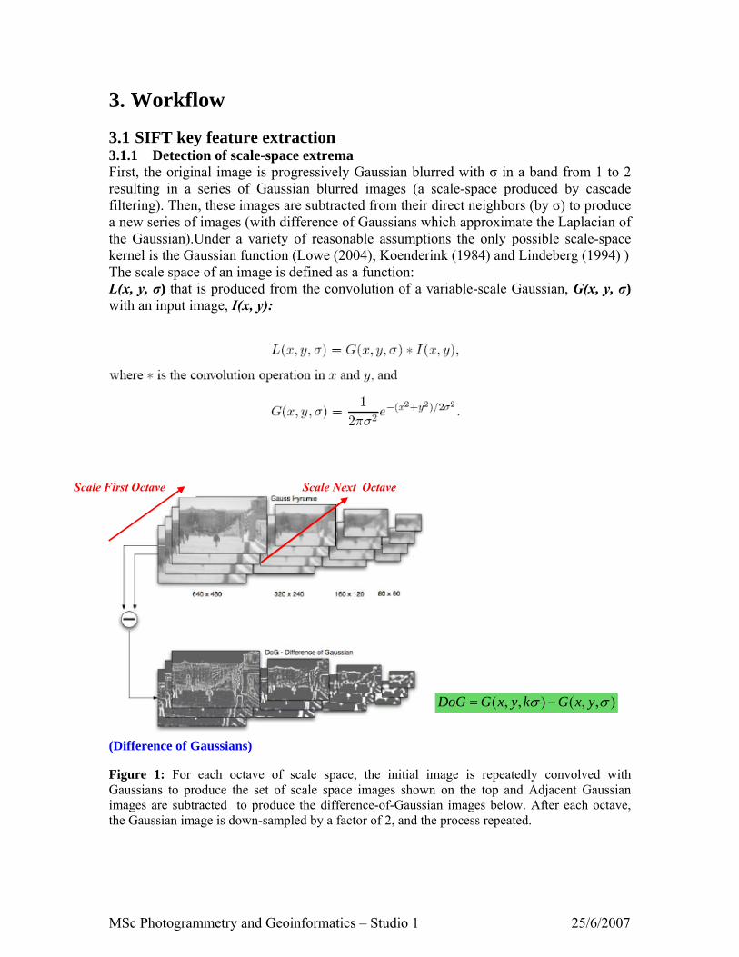
3. Workflow 3.1 SIFT key feature extraction 3.1.1 Detection of scale-space extrema First, the original image is progressively Gaussian blurred with σ in a band from 1 to 2 resulting in a series of Gaussian blurred images (a scale-space produced by cascade filtering). Then, these images are subtracted from their direct neighbors (by σ) to produce a new series of images (with difference of Gaussians which approximate the Laplacian of the Gaussian).Under a variety of reasonable assumptions the only possible scale-space kernel is the Gaussian function (Lowe (2004), Koenderink (1984) and Lindeberg (1994) ) The scale space of an image is defined as a function: L(x, y, σ) that is produced from the convolution of a variable-scale Gaussian, G(x, y, σ) with an input image, I(x, y):

(Difference of Gaussians)

Scale Next OctaveScale First Octave

( , , ) ( , , )DoG G x y k G x yσ σ= −

Figure 1: For each octave of scale space, the initial image is repeatedly convolved with Gaussians to produce the set of scale space images shown on the top and Adjacent Gaussian images are subtracted to produce the difference-of-Gaussian images below. After each octave, the Gaussian image is down-sampled by a factor of 2, and the process repeated.

MSc Photogrammetry and Geoinformatics – Studio 1 25/6/2007

To efficiently detect stable keypoint locations in scale space, (Lowe, 1999)a scale-space extrema in the difference-of-Gaussian function convolved with the image,D(x, y, σ) is computed from the difference of two nearby scales separated by a constant multiplicative factor k:

Difference of Gaussian (DOG),which is, coarsely speaking, the scale derivative of the Gaussian scale space.

Figure2 Maxima and minima of the difference-of-Gaussian images are detected by comparing a pixel (marked with X) to its 26 neighbors in 3x3 regions at the current and adjacent scales (marked with circles) as shown in the figure2. 3.1.2 Accurate Keypoint localization Once a keypoint candidate has been found by comparing a pixel to its neighbors, the next step is to perform a detailed fit to the nearby data for location, scale, and ratio of principal curvatures. This information allows points to be rejected that have low contrast (and are therefore sensitive to noise) or are poorly localized along an edge. Using Taylors Expansion for fitting 3D quadratic function to the local sample points to determine the interpolated location of the maximum,

And using it for the location of the extremum, ^x, which is determined by taking the derivative of this function with respect to x and setting it to zero, giving

Then substituting 3 into 2 gives us:

MSc Photogrammetry and Geoinformatics – Studio 1 25/6/2007

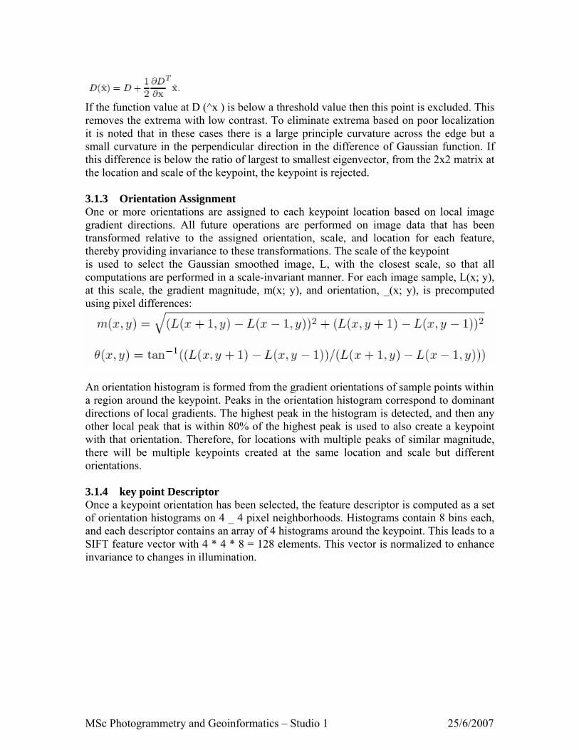
If the function value at D (^x ) is below a threshold value then this point is excluded. This removes the extrema with low contrast. To eliminate extrema based on poor localization it is noted that in these cases there is a large principle curvature across the edge but a small curvature in the perpendicular direction in the difference of Gaussian function. If this difference is below the ratio of largest to smallest eigenvector, from the 2x2 matrix at the location and scale of the keypoint, the keypoint is rejected. 3.1.3 Orientation Assignment One or more orientations are assigned to each keypoint location based on local image gradient directions. All future operations are performed on image data that has been transformed relative to the assigned orientation, scale, and location for each feature, thereby providing invariance to these transformations. The scale of the keypoint is used to select the Gaussian smoothed image, L, with the closest scale, so that all computations are performed in a scale-invariant manner. For each image sample, L(x; y), at this scale, the gradient magnitude, m(x; y), and orientation, _(x; y), is precomputed using pixel differences:

An orientation histogram is formed from the gradient orientations of sample points within a region around the keypoint. Peaks in the orientation histogram correspond to dominant directions of local gradients. The highest peak in the histogram is detected, and then any other local peak that is within 80% of the highest peak is used to also create a keypoint with that orientation. Therefore, for locations with multiple peaks of similar magnitude, there will be multiple keypoints created at the same location and scale but different orientations. 3.1.4 key point Descriptor Once a keypoint orientation has been selected, the feature descriptor is computed as a set of orientation histograms on 4 _ 4 pixel neighborhoods. Histograms contain 8 bins each, and each descriptor contains an array of 4 histograms around the keypoint. This leads to a SIFT feature vector with 4 * 4 * 8 = 128 elements. This vector is normalized to enhance invariance to changes in illumination.

MSc Photogrammetry and Geoinformatics – Studio 1 25/6/2007

Matlab procedure for sift feature extraction: Lowe himself has released a program named “Invariant Keypoint Detector,” which analyzes an input image and outputs a file containing the keypoint descriptors of the SIFT features found in that image. Presumably, this program implements the algorithm as described in Lowe’s papers, although since the source is unavailable, we have no way of knowing for certain what it is doing. We used this code for generating the sift key features. (source: http://www.cs.ubc.ca/spider/lowe/research.html ) [im1, des1, loc1] = sift(image1); Below figures shows the keyfeatures generated on images using SIFT algorithm.

Keyfeatures in Reference image Key features in Candidate

Image

MSc Photogrammetry and Geoinformatics – Studio 1 25/6/2007

4. Keypoint Matching ng between key points in the candidate image to the

iant

Precompute matrix transpose

t

k if nearest neighbor has angle less than distRatio times 2nd.

figure shows the matched points.

Our next task was to do the matchidatabase of keypoints generated from the reference image. The best candidate match for each keypoint is found by identifying its nearest neighbor in the database of keypoints from training images. The nearest neighbor is defined as the keypoint with minimum Euclidean distance for the invariant descriptor vector. The inverse cosine function of the dot product of key descriptors from candidate image and reference image is calculated. This will give you a approximate measure of Euclidian distance. Then the distance ratio of nearest neighbour to the second nearest neighbour for all the possible combinations are calculated . Then a threshold of 0.6 is applied to eliminate false matches. The matlab procedure for the above application is given below.

invarkey descriptors - a K-by-128 matrix, where each row gives andescriptor for one of the K keypoints. The descriptor is a vector

of 128 values normalized to unit length. des2t = des2'; % for i = 1 : size(des1,1) dotprods = des1(i,:) * des2t; % Computes vector of doproducts [vals,indx] = sort(acos(dotprods)); % Take inverse cosine and sort results

% Chec if (vals(1) < distRatio * vals(2))

match(i) = indx(1); else match(i) = 0;

endend Below

MSc Photogrammetry and Geoinformatics – Studio 1 25/6/2007

5. Removing Outliers

After Matching we get some false matches which we need to eliminate for the further object recognition process. In this case we employed RANSAC(Random Sample Consensus) as our robust fitting method to remove our outliers. RANSAC iteratively generates model from a random subset of the original data and check how much other data fits to the model. From the best fit model it get the inliers. Here for our purpose we used Ransac-fit-homography which Robustly fits a homography to a set of matched points.

The MATLAB procedure to call RANSAC is given below

%Calling ransacfithomography [H, inliers] = ransacfithomography(x1, x2, t); x1t=x1'; x2t=x2'; M1=x1t(inliers,:); =x2t(inliers,:);

elow figure shows the best matched points after applying RANSAC. M2B

MSc Photogrammetry and Geoinformatics – Studio 1 25/6/2007

6. Affine Transformation We need to overlay the reference image on the identified object in the candidate image. For that we used affine transformation . The transformation parameters to do this is generated by the function cp2tforn with the correct matches from RANSAC as our input control points.These parameters are used in the function imtransform to finally transform the image. The MATLAB procedure for the above task is given below. tform = cp2tform(M1,M2,'affine') transformed = imtransform(im1rgb,tform,... Below figure shows the transformed image overlayed on candidate image.

MSc Photogrammetry and Geoinformatics – Studio 1 25/6/2007

Examples and Conclusions: 1.

Reference Image

Candidate Image

After Matching

Rod: 626 keypoints found Image: 2347 keypoints found Matches: 155

Red lines represents outliers and cyan represents inliers.

MSc Photogrammetry and Geoinformatics – Studio 1 25/6/2007

After RANSAC.

Matches: 144

Above figure , Outliers have been eliminatedAffine Transformation.

.

Above example we were able to get a lot of good matches because of the good quality of

be identified was clearly visible ion. The object in both the images had distinct texture pattern, which

attributed to the perfect match.

the image with less objects and clutter. Also the object towithout any occlus

MSc Photogrammetry and Geoinformatics – Studio 1 25/6/2007

2. Candidate Image

Reference Image

After Matching

Rod: 626 keypoints found Image: 17927 keypoints found Matches: 16

Red lines represents outliers and cyan represents inliers.

MSc Photogrammetry and Geoinformatics – Studio 1 25/6/2007

After RANSAC.

Above figure, Outliers have been eliminated.

ation Affine Transform

The result of the example2 is not impressive, as the algorithm failed to match conjugate points. This can be attributed to the fact that the rod in the candidate image had extensive features more than the size of the reference rod and in addition the higher distance to the camera viewpoint might have affected the result. So we can say that the performance will ary with the scale variations to some limits. IFT algorithm generates features which are robust to occlusion and clutter. Individual atures can be matched to a large database of features. It is a efficient algorithm in terms

small objects.

vSfeof time and also generates more unique features for even

MSc Photogrammetry and Geoinformatics – Studio 1 25/6/2007

Reference: Lowe, D.G. 1999. Object recognition from local scale-invariant features. In

International Conference on Computer Vision, Corfu, Greece, pp. 1150-1157. Lowe, D.G. 2003. Distinctive image features from scale-invariant keypoints. Draft

submitted for publication. http://www.cs.ubc.ca/spider/lowe/research.html http://www.csse.uwa.edu.au/~pk/research/matlabfns/ http://homepages.inf.ed.ac.uk/rbf/CVonline/LOCAL_COPIES/AV0405/MURRAY/SIFT.html Gulch, E 2007. lecture notes, MSc Photogrammetry and Geoinformatics, hft-Stuttgart

etry and Geoinform tics, hft-Stuttgart

Hahn, M 2007. lecture notes, MSc Photogramm a

MSc Photogrammetry and Geoinformatics – Studio 1 25/6/2007