Supplementary Information

Designing the Next-Generation of High Capacity Battery Electrodes

Hui-Chia Yu1, Chen Ling1, Jishnu Bhattacharya1, John C. Thomas1, Katsuyo Thornton1,

Anton Van der Ven1,2*

1Department of Materials Science and Engineering, University of Michigan, Ann Arbor,

MI 48109, USA

2Materials Department, University of California Santa Barbara, CA. 93106-5050, USA

* avdv@engineering.ucsb.edu

I. First-principles and Monte Carlo calculations

I.A. First-principles calculation of thermodynamic properties

The thermodynamic properties for the Li-Cu-TiS2 ternary system within the spinel crystal

structure of TiS2 were calculated with well-established statistical mechanical techniques

based on the cluster expansion formalism [1,2] as implemented in our CASM (A clusters

approach to statistical mechanics) code [3,4]. The approach relies on the construction of an

effective Hamiltonian (a cluster expansion) that describes the energy of the crystal as a

function of configurational degrees of freedom. The coefficients of the effective Hamiltonian

are fit to first-principles total energy calculations obtained within the generalized gradient

approximation (GGA) to density functional theory (DFT). Monte Carlo simulations are then

applied to calculate finite temperature thermodynamic properties, including relationships

between free energies, chemical potentials and concentrations.

To mathematically represent the ternary configurational degrees of freedom

associated with all the possible ways of distributing Li, Cu and vacancies over the interstitial

sites of spinel TiS2 (i.e. the 8a and 16c sites within the Fd3m space group, with Ti and S

occupying the 16d and 32e sites respectively), we assign occupation variables to each

interstitial site. First-principles total energy calculations show that Li is stable in both the

octahedral and tetrahedral sites of spinel TiS2, energetically preferring the octahedral sites [5]

, while Cu only occupies the tetrahedral sites. Hence, the octahedral sites will only have

1

Electronic Supplementary Material (ESI) for Energy & Environmental Science.This journal is © The Royal Society of Chemistry 2014

binary disorder (Li-vacancy) while the tetrahedral sites will have ternary disorder (Cu, Li and

vacancies). For each octahedral site, we assign an occupation variable

piLi that is equal to 1 if

site i is occupied by Li and 0 if it is vacant. For each tetrahedral site, we assign two

occupation variables, p jLi and p j

Cu . Just as with the octahedral site, p jLi for the tetrahedral

site is equal to 1 if site j is occupied by Li and 0 otherwise, and p jCu is equal to 1 if site j is

occupied by Cu and 0 otherwise. Within the cluster expansion formalism, the total energy

can then be written as an expansion in terms of products of occupation variables belonging to

clusters of sites according to

E p Vo V p

(S1)

where

p p1Li,..., pi

Li,..., p2NLi , p1

Cu,..., p jCu,..., pN

Cu is the collection of occupation variables for a

spinel crystal structure of TiS2 having 2N octahedral sites and N tetrahedral sites. The

polynomial basis functions are defined as products of occupation variables belonging to a

cluster of sites within the crystal according to

piA

i

(S2)

where i are tetrahedral or octahedral sites belonging to a cluster (e.g. a pair cluster, a

triplet, a quadruplet etc.), and A refers to either Li or Cu. The coefficients in the above cluster

expansion, Vo and V, are called effective cluster interactions and are to be determined from

first principles. While the cluster expansion extends over all clusters of sites and

permutations of Li and Cu occupation variables over those sites, in practice, it must be

truncated above some maximally sized cluster.

The effective cluster interactions (ECI) are usually fit to reproduce the total energies,

calculated from first principles, for a number of different configurations. In this work, DFT

calculations were performed with the Vienna ab initio simulation package (VASP) [6,7]

using the generalized gradient approximation with the projector augmented-wave (PAW)

functional [8,9] and a cutoff energy of 400.0 eV for the electron plane wave expansion. All

ions and the shape and size of the supercells of different Li-Cu-vacancy configurations

within spinel TiS2 were allowed to relax until the forces on all atoms were less than 0.03

2

eV/Å. We used the TiS2, Cu0.5TiS2 and LiTiS2 as the reference state. The cluster expansion

was fit to the formation energies of LixCuyTiS2 defined as:

E f Et,LixCuyTiS2 xEt,LiTiS2

yEt,Cu0.5TiS2 (1 x y)Et,TiS2

(S3)

where

E t,LixCuyTiS2,

E t,LiTiS2,

E t,Cu0.5TiS2 and

E t,TiS2 are the total energies of LixCuyTiS2, LiTiS2,

Cu0.5TiS2 and spinel TiS2, respectively. A total of 256 Li-Cu-vacancy configurations over

spinel TiS2 were calculated and used in the fit of the ECI of a truncated cluster expansion.

The cluster expansion contains 8 Li-Li pairs, 18 Li-Li-Li triplets, and 15 Li-Li-Li-Li

quadruplets, 6 Cu-Cu pairs, 3 Cu-Cu-Cu triplets and 1 Cu-Cu-Cu-Cu quadruplet along with 7

Li-Cu pairs and 1 Li-Cu triplet interaction. The ability of the cluster expansion fit to

reproduce the original energies is illustrated in Fig. S1. The root mean square error is 3.2

meV per LixCuyTiS2 formula unit.

Figure S 1 The cluster expansion fitted formation energies (Ef) versus the formation energies calculated by DFT for the same configuration.

Grand Canonical Monte Carlo simulations were performed in a spinel crystal with

periodic boundary conditions containing 121212 spinel primitive cells. The average

composition of Li and Cu was calculated as a function of chemical potential. The grand

3

canonical and Gibbs free energies were subsequently obtained through free energy

integration in ternary chemical potential space [10] using the energies of TiS2, Cu0.5TiS2 and

LiTiS2 as the reference states. The ternary phase diagram was then calculated by determining

the crossing points of the grand canonical free energies determined from Monte Carlo

simulations that traversed from low to high chemical potential and from high to low chemical

potential. Hysteresis in Monte Carlo simulations around first-order phase transitions (two-

phase regions in the present context) allows us to calculate meta-stable free energies that

extend into the two-phase regions to some degree. Crossing points of grand canonical free

energies as a function of chemical potentials are equivalent to the common tangent

construction applied to the Gibbs free energy. While LixCuyTiS2 exhibits a variety of stable

ordered phases at zero Kelvin, our Monte Carlo simulations indicated that Li and Cu form a

disordered solid solution over the interstitial sites of spinel TiS2 at 300 K. We found no

evidence of Li-Cu-vacancy ordering at room temperature as manifested by steps in the

chemical potential curves as a function of concentration. We did not explore order-disorder

reactions below 300 K.

The free energy obtained from first principles and Monte Carlo simulations is only

defined for regions in the TiS2-Cu0.5TiS2-LiTiS2 ternary composition space where the solid

solution is stable or metastable. Regions where the curvature of the free energy surface is

negative (i.e. the solid solution is unstable) are inaccessible with Monte Carlos simulations.

The free energy inside the spinodal was therefore described with a downward parabolic

surface for the two-phase region. The free energy within the spinodal was parameterized such

that appropriate interfacial energy and interfacial thickness of the phase boundary are

determined along with the gradient energy coefficient as

~ (2 2h ) /3 and l ~ / 2h

respectively, where is the gradient energy coefficient and h is the barrier height of the free

energy function. Here, we set the height of the downward parabolic surface to be 0.09 eV.

The selection of this value was motivated by first-principles calculated mixing energies. The

Li-octahedra share faces with the Cu-tetrahedra in the spinel host of TiS2. Along the

Cu0.5TiS2-LiTiS2 composition line, Li and Cu will by necessity occupy octahedral and

tetrahedral sites that share faces, which has a large energy penalty associated with it. For

example, the mixing energy for Li2Cu(TiS2)4 relative to Cu0.5TiS2 and LiTiS2 whereby Li and

Cu are arranged to minimize the number of filled face-sharing Cu tetrahedra and Li octahedra

4

was calculated to be 0.09 eV per formula unit. Other configurations that increase the number

of shared tetrahedron/octahedron faces have higher mixing energies.

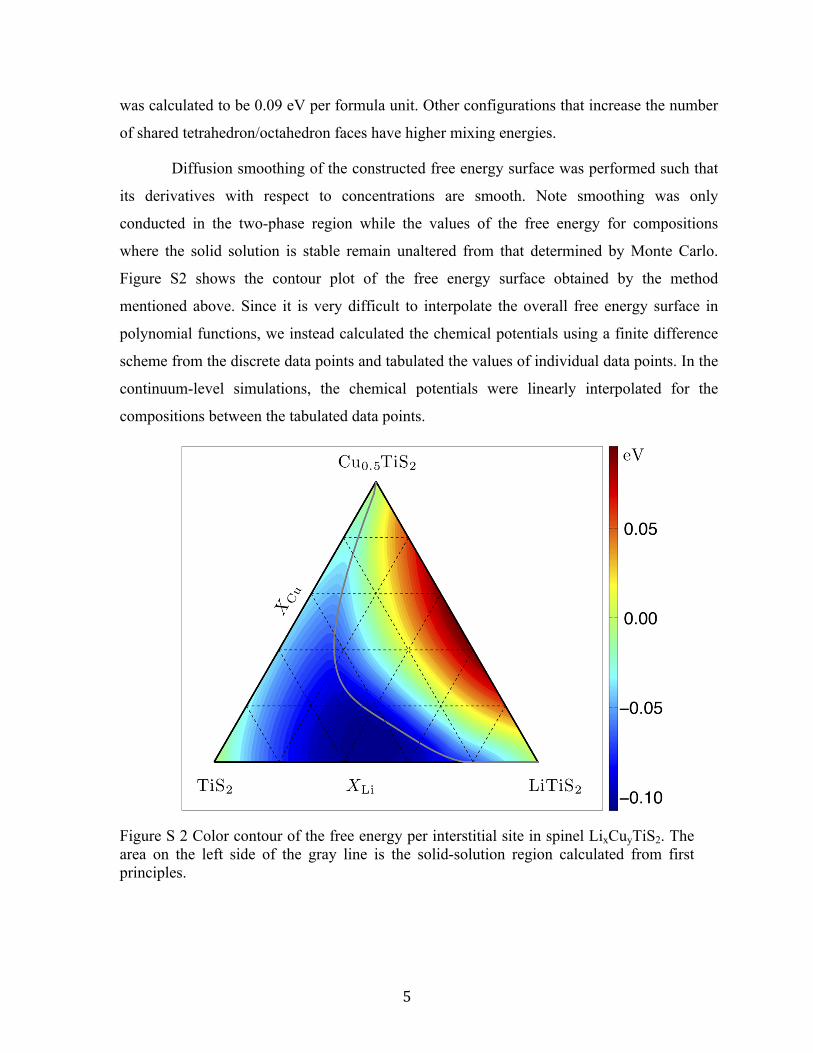
Diffusion smoothing of the constructed free energy surface was performed such that

its derivatives with respect to concentrations are smooth. Note smoothing was only

conducted in the two-phase region while the values of the free energy for compositions

where the solid solution is stable remain unaltered from that determined by Monte Carlo.

Figure S2 shows the contour plot of the free energy surface obtained by the method

mentioned above. Since it is very difficult to interpolate the overall free energy surface in

polynomial functions, we instead calculated the chemical potentials using a finite difference

scheme from the discrete data points and tabulated the values of individual data points. In the

continuum-level simulations, the chemical potentials were linearly interpolated for the

compositions between the tabulated data points.

Figure S 2 Color contour of the free energy per interstitial site in spinel LixCuyTiS2. The area on the left side of the gray line is the solid-solution region calculated from first principles.

5

I.B. Calculation of diffusion coefficients

Diffusion in electrode particles undergoing displacement reactions is more complex than

simple intercalation as two components must diffuse over the interstitial sites of the host. For

example Li and Cu diffusion can occur simultaneously in solid solutions of LixCuyTiS2,

sharing interstitial sites of the spinel TiS2 network. From irreversible thermodynamics, the

relevant flux equations take the form

JLi LLiLiLi LLiCuCu (S4a)

JCu LCuLiLi LCuCuCu (S4b)

where Lij are the kinetic transport coefficients and i are chemical potentials. The coefficients

Lij can be calculated using Kubo-Green expressions according to [11,12,13]

Lij

R

i t

R

j t

2d tVkBT (S5)

where

R

i t connects the endpoints of trajectories of atom of type i = Li or Cu after time t

in a crystal of volume V, kB is Boltzmann’s constant, T is the absolute temperature and d is

the dimension of the network of interstitial sites. The triangular brackets denote averages in

the usual statistical mechanical sense. It is more practical to express the fluxes in terms of

gradients of concentration

JLi DLiLiCLi DLiCuCCu (S6a)

JCu DCuLiCLi DCuCuCCu (S6b)

where the matrix of diffusion coefficients Dij is a matrix product of Lij with a matrix of partial

derivatives of chemical potentials. As with simple intercalation, all quantities needed to

determine the matrix of diffusion coefficients can be calculated by applying grand canonical

Monte Carlo simulations (to obtain chemical potentials versus composition) and kinetic

Monte Carlo simulations (to evaluate kinetic transport coefficients) to cluster expansions for

the configurational energy and migration barriers.

The Kubo-Green expressions can be evaluated explicitly by sampling a large number

of representative trajectories within kinetic Monte Carlo simulations. These can be sampled

with transition state theory providing stochastic estimates of hop frequencies of atoms to

adjacent vacant sites. According to Vineyard [14], these hop frequencies can be estimated as

6

*exp EkBT

(S7)

where E is the migration barrier for a hop and * is a vibrational prefactor, which in the

Harmonic approximation, is equal to the ratio of the product of vibrational frequencies of the

solid in the initial state to the product of non-imaginary vibrational frequencies of the solid

when the atom is in the activated state.

Due to the large difference between the calculated Li and Cu mobilities in spinel TiS2

(with typical hop frequencies differing by several orders of magnitude at room temperature)

it is not feasible with standard kinetic Monte Carlo simulations to evaluate the full 22

matrix of kinetic transport coefficients Lij. Hence in this study we restricted ourselves to

predicting diffusion coefficients along the binary TiS2-Cu0.5TiS2 and TiS2-LiTiS2 axes and

then extrapolating these values to the ternary space as described below. For single component

interstitial diffusion, the diffusion coefficients appearing in Fick’s law can be factored into a

product of a thermodynamic factor, , and a kinetic factor, DJ, according to D DJ [15]

with

DJ kBT

XL and

/ kBT ln X

(S8)

where L is a kinetic transport coefficient obtained using the method as in Eq. (S5), is the

volume of the host per interstitial site available, and X is the occupied site fraction of the

diffusion species.

The calculation of the Li diffusion coefficient is described in more detail elsewhere [16,

17,18]. All migration barriers were calculated in the cubic unit cell of spinel TiS2 consisting

of 32 sulfur atoms, 16 titanium atoms and variable number of Li or Cu atoms. The nudged

elastic band method was used to calculate the migration barrier for Li and Cu hops. A

calculation of 30 migration barriers in different Li-vacancy configurations revealed a strong

dependence of the barrier on local environment. However, this dependence was only on the

immediate local environment, with migration barriers for leaving tetrahedral sites lying in

three distinct bands depending on whether the Li atom was hopping into a single vacancy, a

divacancy or a triple vacancy [5]. The migration barriers for 8 different Cu-vacancy

configurations were also calculated in TiS2. The Cu migration barriers were found to be

7

insensitive (within the numerical error of these calculations, ~25-50 meV) to Cu composition

and Cu-vacancy arrangement, having a value around 0.9 eV. Within the kinetic Monte Carlo

simulations, the cluster expansion for Li-Cu-vacancy disorder over the interstitial sites of

spinel TiS2 was used to calculate the energies of the end states of the hop. For Li hops,

migration barriers were calculated by adding environment dependent barriers to the energy of

tetrahedral occupancy [5]. For Cu hops, a constant kinetically resolved migration barrier was

added to the average energy of the intial and final states of the hop minus the energy of the

initial state of the hop [16]. The vibrational prefactors appearing in Vineyard’s expression for

atomic hop frequencies were calculated within the local harmonic approximation. Predicted

Li and Cu diffusion coefficients along the TiS2-Cu0.5TiS2 and TiS2-LiTiS2 binary axes are

shown in Fig. 2c in the main text.

Calculations of the migration barriers for Li and Cu as a function of the spinel TiS2

host volume showed that the Li migration barrier increased with decreasing volume while

that of Cu decreased with decreasing volume. Since all calculations were performed within

the GGA approximation to DFT, which over predicts lattice parameters, we expect that the

predicted mobility of Cu is likely underestimated while that of Li is overestimated. For

example, we found that the migration barrier of Cu at the equilibrium GGA lattice parameter

of TiS2 (9.83 Å) is almost 100 meV higher than that calculated at the experimental lattice

parameter of TiS2 (9.75 Å). At room temperature, the difference in migration barriers

translates into an underprediction of the Cu diffusion coefficient by a factor of 50 (almost 2

orders of magnitude).

We used the calculated diffusion coefficients of the TiS2-Cu0.5TiS2 and TiS2-LiTiS2

binaries to estimate the diagonal L coefficients for the ternary system. The diagonal Lii

coefficients scale directly with the concentration of the diffusing specie i. Furthermore, if the

interstitial sites form a lattice and the interstitial atoms behave as an ideal solution, the kinetic

transport coefficients will also scale with the concentration of vacancies [19]. For Li and Cu

diffusion in spinel TiS2, we can therefore to first order write the diagonal transport

coefficients for ternary compositions as

LLiLi XLi 1 XLi 1 2XCu Li (S9a)

LCuCu XCu 1 XLi 1 2XCu Cu . (S9b)

8

Since the Li and Cu atoms do not occupy the same sublattice, the kinetic coefficients scale

with the vacancy concentration on each sublattice. For example, Li hops require the end state

of the hop on the octahedral site to be vacant. However, since Li must hop through a

tetrahedral site, the intermediate tetrahedral site must also be vacant. Hence,

LLiLi should

scale with the product of the vacancy concentration on the tetrahedral sublattice, 1 2XCu ,

and the vacancy concentration on the octahedral sublattice, 1 XLi . In the above expressions,

Li and Cu will also depend on the overall concentration, XLi and XCu, if the migration

barriers for the hops depend on concentration and if hop frequencies depend on long and

short-range order among the interstitial diffusers (e.g. the divacancy and triple-vacancy hop

mechanisms for Li in spinel LixTiS2). In extrapolating our binary diffusion coefficients to the

ternary system, we fit Li and Cu such that the diagonal kinetic transport coefficients

reproduce the binary kinetic transport coefficients. The mobilities, i, are related to the self-

diffusion coefficients calculated from first principles and kinetic Monte Carlo simulations

according to

Li DJ

Li

1 XLi kBT and Cu

DJCu

1 2XCu kBT(S10)

where

DJLi and

DJCu are the binary self-diffusion coefficients of Li and Cu in TiS2 crystal,

respectively. Note that we have neglected the off-diagonal terms in the Onsager transport

coefficients in Eq. (S4), and similarly those in the boundary conditions (insertion/extraction

fluxes). While it is a reasonable approximation for most materials, there could be examples,

where such approximations are not valid and our general conclusion may not hold.

Substituting Eq. (S10) into Eq. (S9), we obtain

LLiLi XLi 1 2XCu a DJ

Li

kBT (S11a)

LCuCu XCu 1 XLi b DJ

Cu

kBT (S11b)

where a and b are small values taken to avoid a complete stall in diffusion in the

simulations. Here, we choose 0.00025 and 0.000125 for a and b , respectively. They are

0.1% of the maximum values of XLi 1 2XCu and XCu 1 XLi .

9

As a measure of the asymmetry in Li and Cu mobilities, we defined a parameter, , to

be DLi / DCu , where DLi and DCu are the average value of the diffusion coefficients,

respectively, over the single-component axes in the composition space; i.e.,

DLi DLi XLi 0

1

dXLi / dXLi0

1

and DJCu DCu XCu

0

0.5

dXCu / dXCu0

0.5

. When the value of is

unity, the mobilities are equal on average, while greater than one indicates Li is more

mobile than Cu on average. A similar parameter averaging the transport coefficient can be

obtained by L LLiLi / LCuCu , where the average values of transport coefficients are taken

over the ternary composition space as

LLiLi LLiLi XLi, XCu 0

1XLi /2 dXCu0

1

dXLi / dXCu0

1XLi /20

1

dXLi and

LCuCu LCuCu XLi, XCu 0

1XLi /2 dXCu0

1

dXLi / dXCu0

1XLi /20

1

dXLi . In this presented work, the

values of L scales with by L 0.8749 .

II. Phase field approach

II.A. Cahn-Hilliard equation

In a phase field model, the chemical potential for transport is given by

fC2C (S12)

where f is the bulk free energy (described below), C is the order parameter, and is the

gradient energy coefficient. For a conserved order parameter (e.g., concentration), the flux is

given by J L , where L is the transport mobility, and the gradient of the chemical

potential provides the driving force. The concentration evolution is governed by mass

conservation:

Ct L f

C2C

. (S13)

This equation is known as the Cahn-Hilliard equation. When f has two minima, as in a

double-well function, the system tends to separate into two phases (or stay in a two-phase

coexistence mixture). This is the case when the composition resides in the two-phase region

in the ternary phase diagram shown in the main text. The second term in the chemical

10

potential panelizes a steep variation of the composition in the interfacial region, and, along

with the excess bulk free energy, contributes to the interfacial energy. On the other hand,

when f has a single minimum, the system tends to form a single-phase solid solution. This is

the case when the composition is in the solid solution region in the ternary phase diagram.

II.B. Smoothed boundary method

To account for the particle geometry in the simulations, we employed the smoothed boundary

method [20,21] with a continuous domain parameter, . The region within the particle where

Li and Cu transport occurs is defined by volume where

1, while the outside of the

particle is defined by

0. Therefore, the particle surface where Li and Cu are

inserted/extracted is automatically defined by the narrow transitioning region where

0 1. The Cahn-Hilliard equations for Li and Cu are then reformulated [21] into

CLi

t

1 LLiLiLi

JLi s (S14a)

CCu

t

1 LCuCuCu

JCu s (S14b)

where JLi s and JCu s are the insertion/extraction fluxes at the particle surface for Li and Cu,

respectively, and their expressions are given in the main text.

II.C. Simulation setup

The concentration evolution equations were nondimensionalized by using the length scale l,

the reference mobility L0, and time scale

l2 /L0. A standard second-order central

difference scheme in space and Euler explicit scheme in time were employed to implement

the 2D continuum-level simulations. The 2D computational domain contains 176128

Cartesian grid points, which corresponds to an area of 1.761.28 m2. Particle geometry was

defined by a continuous domain parameter, , where

1 for the interior of the particle and

0 for the exterior. The long and short axes of the particle are roughly 150 and 105 grid

spacings, respectively. The domain parameter takes the form of

11

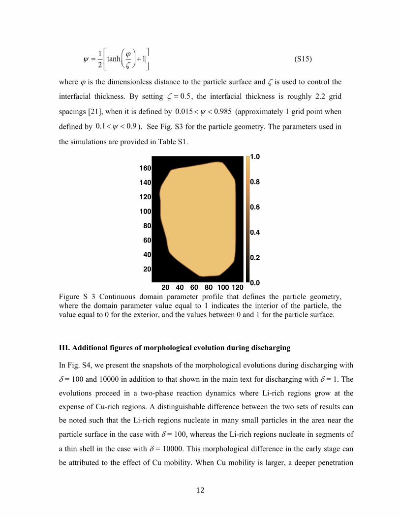
12

tanh 1

(S15)

where is the dimensionless distance to the particle surface and is used to control the

interfacial thickness. By setting 0.5 , the interfacial thickness is roughly 2.2 grid

spacings [21], when it is defined by 0.015 0.985 (approximately 1 grid point when

defined by 0.1 0.9 ). See Fig. S3 for the particle geometry. The parameters used in

the simulations are provided in Table S1.

Figure S 3 Continuous domain parameter profile that defines the particle geometry, where the domain parameter value equal to 1 indicates the interior of the particle, the value equal to 0 for the exterior, and the values between 0 and 1 for the particle surface.

III. Additional figures of morphological evolution during discharging

In Fig. S4, we present the snapshots of the morphological evolutions during discharging with

= 100 and 10000 in addition to that shown in the main text for discharging with = 1. The

evolutions proceed in a two-phase reaction dynamics where Li-rich regions grow at the

expense of Cu-rich regions. A distinguishable difference between the two sets of results can

be noted such that the Li-rich regions nucleate in many small particles in the area near the

particle surface in the case with = 100, whereas the Li-rich regions nucleate in segments of

a thin shell in the case with = 10000. This morphological difference in the early stage can

be attributed to the effect of Cu mobility. When Cu mobility is larger, a deeper penetration

12

length for Cu is reached, resulting in spherical initial Li-rich phases. In contrast, plate-like

initial Li-rich phases form when Cu mobility is small. The Li-rich regions continuously grow

and eventually form a complete shell of the particle. Once the shells are completed. The

following morphological evolutions for both the two cases are very similar; i.e., a shrinking-

core phase boundary motion until the entire particles are lithiated. Although with a

discernible difference in the nucleation and early stages of the morphological evolutions, the

kinetic reaction paths of discharge for both the two cases, as well as the case with = 1, all

follow the same edge (Cu0.5TiS2-LiTiS2) in Fig. 6A in the main text, showing the same two-

phase transition from Cu-rich Cu0.5TiS2 to Li-rich LiTiS2. This is because Li can only enter

the crystal when Cu is extruded despite Cu mobility and the corresponding morphology. The

simulations clearly demonstrate that the reaction path of discharge is independent of mobility

asymmetry between Li and Cu in this displacement reaction.

Figure S 4 Snapshots of evolution of Li and Cu in the LixCuyTiS2 particle during discharge process for (a)-(d) = 100 and (e)-(h) = 10000. The left and right images in each subfigure are Li and Cu mole fraction profiles, respectively, in the same particle at the same time. The average compositions of the entire particle in (a)-(d) and (e)-(h) are

= (0.0625, 0.469), (0.125, 0.438), (0.25, 0.375), and (0.375, 0.3125), (X̅Li, X̅Cu)respectively.

13

Table S 1 The physical parameters used in the continuous simulations.

Grid spacing (l) 10-6 cmReference mobility (L0) 110-9 s-1cm-1eV-1

Reaction constant for Li (KLi) 210-3 s-1cm-2eV-1

Reaction constant for Cu (KCu) 210-3 s-1cm-2eV-1

Gradient coefficient for Li (Li) (eV)1/2lGradient coefficient for Cu (Cu) (eV)1/22lApplied voltage for discharge () 1.0 VApplied voltage for charge () 2.4 V

1 J. M. Sanchez, F. Ducastelle, D. Gratias, Physica A, 128, 334-350 (1984).

2 D. de Fontaine, Solid State Physics, 47, 33-176 (1994).

3 A. Van der Ven, J. C. Thomas, Qingchuan Xu, B. Swoboda, D. Morgan, Physical Review B 78, 104306 (2008).

4 A. Van der Ven, J. C. Thomas, Q. Xu, J. Bhattacharya, Mathematics and Computers in Simulation, 80(7) 1393-1410 (2010).

5 J. Bhattacharya, A. Van der Ven, Physical Review B, 83, 144302 (2011).

6 G. Kresse, J. Furthmuller, Comput. Mater. Sci., 6, 15 (1996).

7 G. Kresse, J. Furthmuller, Phys. Rev. B, 54, 11169 (1996).

8 P. E. Blochl, Phys. Rev. B, 50, 17953, (1994).

9 G. Kresse, J. Joubert, Phys. Rev. B, 59, 1758 (1999).

10 Q. Xu, A. Van der Ven, Intermetallics, 17 (5), 319-329 (2009).

11 A. R. Allnatt, A. B. Lidiard “Atomic transport in solids” Cambridge, Cambridge University Press; (1993).

12 R. Zwanzig, J. Chem. Phys. 40(9), 2527 (1964).

13 A. Van der Ven, H. C. Yu, G. Ceder, K. Thornton, Progress in Materials Science, 55 (2), 61-105 (2010).

14 G. H. Vineyard, J. Physics and Chemistry of Solids 3, 121, (1957).

15 R. Gomer, Reports on progress in physics 53(7), 917-1002, (1990).

16 A. Van der Ven, G. Ceder, M. Asta, P. D. Tepesch, Physical Review B 64, 184307, (2001).

17 A. Van der Ven, J. C. Thomas, Qingchuan Xu, B. Swoboda, D. Morgan, Physical Review B, 78, 104306 (2008)

18 A. Van der Ven, J. Bhattacharya, A. A. Belak, Acc. Chem. Res. (2012), DOI: 10.1021/ar200329r.

19 R. Kutner, Phys. Lett. 81A, 239, (1981)

20 A. Bueno-Orovio, V. M Peres-Garcia, Num. Meth. P. D. E., 28(3), 886, (2006).

21 H.-C. Yu, H.-Y. Chen and K. Thornton, Model. Simul. Mater. Sci. Eng. 20(7), 075008, (2012)

14