design of exponentially weighted moving average control...

Design of Exponentially Weighted Moving

Average Control Charts for Autocorrelated

Processes With Model Uncertainty

Daniel W. Apley and Hyun Cheol Lee

Department of Industrial Engineering Texas A&M University

College Station, TX 77843

([email protected])

Residual-based control charts are popular methods for statistical process control of autocorrelated

processes. To implement these methods, a time series model of the process is required. The model must

be estimated from data, in practice, and model estimation errors can cause the actual in-control average run length to differ substantially from the desired value. This article develops a method for designing residual-based exponentially weighted moving average (EWMA) charts under consideration of the uncer

tainty in the estimated model parameters. The resulting EWMA control limits are widened by an amount

that depends on a number of factors, including the level of model uncertainty.

KEY WORDS: Autoregressive moving average model; Exponentially weighted moving average chart;

Mean shift detection; Residual-based control chart

1. INTRODUCTION

Statistical process control (SPC) is widely used to monitor

and improve quality in industrial processes. Traditional SPC

techniques are based on the assumption that process data are

independent. Significant advances in measurement and data

collection technology?particularly in the area of in-process

sensing?have created the potential for much more frequent

inspection. As a result, autocorrelated data are now common

(Montgomery and Woodall 1997). The run-length properties of

traditional SPC methods like cumulative sum (CUSUM) and X

charts are strongly affected by data autocorrelation, and the in

control average run length (ARL) can be much shorter than in

tended if the autocorrelation is positive (Johnson and Bagshaw

1974; Vasilopoulos and Stamboulis 1978). Consequently, there

has been considerable research in recent years on designing SPC procedures suitable for autocorrelated processes (see, e.g.,

Montgomery and Woodall 1997; Lu and Reynolds 1999; and

the references therein). The most widely investigated methods for SPC of auto

correlated processes are residual-based control charts (e.g., Alwan and Roberts 1988; Apley and Shi 1999; Berthouex,

Hunter, and Pallesen 1978; English, Krishnamurthi, and Sas

tri 1991; Lin and Adams 1996; Lu and Reynolds 1999; Mont

gomery and Mastrangelo 1991; Runger, Willemain, and Prabhu

1995; Superville and Adams 1994; Vander Wiel 1996; Wardell,

Moskowitz, and Plante 1994). One usually assumes that the

process data xt (t is a time index) follow an autoregressive mov

ing average (ARMA) model with AR order p and MA order q, denoted by ARMA(p, q). Using standard time series notation

(see Box, Jenkins, and Reinsel 1994) with the backward shift

operator B defined such that Bxt = xt-\, an ARMA model can

be written as

Xt=*W)a" (1)

where 0(_5) = 1 -0i_9-02#2-OqW, <_>(?) = 1 -<?i_9

02^2-(frpB?, and at is an independently identically dis

tributed (iid), O-mean sequence of random shocks with vari

ance a];. It is assumed that the in-control process mean has

been subtracted, so that xt is O-mean until a shift occurs. For

notational convenience, the results in this article are derived for

ARMA processes, although a straightforward extension to au

toregressive integrated moving average (ARIMA) processes is

discussed in Section 2.

The basic idea behind residual-based charts is to directly monitor the residuals (the one-step-ahead prediction errors)

generated via et = O"1^)^^)**- From (1), et is exactly the

iid sequence at after any initial transients have died out. Thus

traditional Shewhart, CUSUM, and exponentially weighted

moving average (EWMA) control charts can be applied to

the uncorrelated residuals with well-understood in-control run

length properties. In practice, however, the model parameters

{0i : i = 1,2,...,/?}, {Oi : / = 1,2,..., q], and o% must always

be estimated from process data. Using the """

symbol to denote

estimates of the parameters and the resulting ARMA polynomi als, the residuals generated via the estimated model behave as

the ARMA(p + q,p + q) process,

*(fl) *(B)0(B) et =-xt =-au (2)

0(B) 0(_3)*(_5) and are no longer iid.

Suppose that an EWMA of the form yt = (1 ?

k)yt-\ + \eu for some EWMA parameter 0 < X < 1, is applied to the residu

als. Defining v = 1 - ?, the EWMA statistic, yu can be written

as the ARMA(p + q + 1, p + q) process

1-v (1 -

v)Q(B)?(B) yt =--et =-n-at. (3) 1 - vB (l

- vB)?(B)<t>(B)

? 2003 American Statistical Association and the American Society for Quality

TECHNOMETRICS, AUGUST 2003, VOL 45, NO. 3 DO110.1198/004017003000000014

187

188 DANIEL W. APLEY AND HYUN CHEOL LEE

UCL = .64

0.5 [

y?

-0.5

LCL = -.647

100 200 t

300 400 500

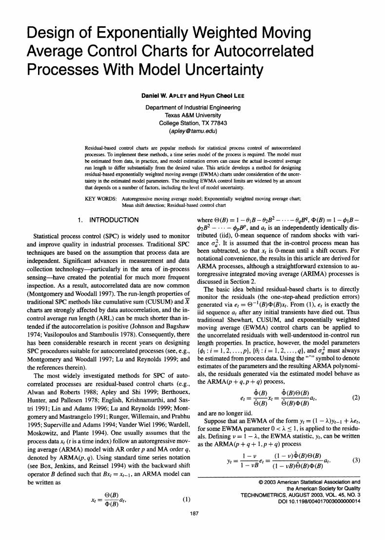
Figure 1. Sample EWMA Chart tor an In-Control AR(1) Process With </> j Underestimated. The desired in-control ARL is 500, whereas the actual ARL is much lower due to frequent false alarms.

For a specified k, the typical EWMA design procedure is to set

the upper control limit (UCL) and lower control limit (LCL) on

yt at (Lu and Reynolds 1999)

{LCL, UCL} = ?L?y, (4)

where ay = oa(\

- v)1/2(l + v)~1/2 is the steady-state standard

deviation of yt assuming that the estimated model is perfect

(Montgomery 2001), and the constant L is chosen to provide a desired in-control ARL. Lucas and Saccucci (1990) devel

oped tables for monitoring iid data that give the values of L

that result in several in-control ARL values for various choices

of k. To improve the sensitivity to mean shifts that occur when

the control chart is first initiated, time-varying control limits

that gradually widen to the steady-state limits (4) can also be

used (Montgomery 2001). This article considers only constant

steady-state control limits.

Let Oy

denote the actual variance of the EWMA statistic (3), which is a function of the true parameters and their estimates.

Because the EWMA is a weighted average of the past residuals, residual autocorrelation due to estimation errors can have a sub

stantial effect on oy and the resulting in-control ARL (Adams and Tseng 1998; Apley and Shi 1999; Lu and Reynolds 1999). If the true and estimated parameters are such that the resid

ual autocorrelation is positive, then ay generally will be larger than ay, the in-control ARL will be shorter than intended, and

the control chart may be plagued with frequent false alarms.

To illustrate the effects of modeling errors, suppose that xt is

an AR(1) process with <?)\ = .9 and a2 = 1.0 and that the esti

mated parameters are $\ = .85 and o%

= 1.0. Using an EWMA

with k = . 1 and treating the estimates as perfect, the assumed

EWMA variance is a2 = a2(l -

v)(l + v)"1 = .053. For a

desired in-control ARL of 500, L = 2.814 (Lucas and Saccucci

1990) and the control limits ?Loy = ?.647 would be used. Us

ing (3) and any of the methods for calculating the variance of

an ARMA process discussed by Box et al. (1994), however, it

can be shown that the actual EWMA variance is Oy = .084?

roughly 60% larger than the assumed variance. If the control

limits based on the assumed variance are used, then Monte

Carlo simulation (refer to Sec. 4 for details) reveals that the

actual in-control ARL is approximately 165, which is substan

tially shorter than intended. Figure 1, which shows the EWMA

statistic for 500 simulated observations with the ?.647 control

limits, illustrates the frequent false alarms that result in this sit

uation.

To account for uncertainty in the estimated parameters and

guard against a situation in which the in-control ARL is sub

stantially shorter than desired, a reasonable precaution is to use

control limits that are wider than those used when the model is

assumed to be perfect. This article presents a method for widen

ing the EWMA control limits based on the following "worst

case" design approach. For a specified k and a given set of

ARMA parameter estimates, (3) implies that oy is a function

of the true, unknown parameters. Considering the uncertainty in the true parameters, Section 2 derives an approximate up

per one-sided 1 ? a confidence interval for cry for some user

selected 0 < a < 1. Let dy^a denote the upper boundary of this

confidence interval, which can be viewed as a worst-case (max

imum) value for the true EWMA standard deviation.

The proposed method is to monitor the EWMA statistic (3), but to use the worst-case control limits,

{LCL,UCL} = ?La3;,a, (5)

instead of the standard control limits (4). Section 3 discusses

guidelines for selecting the design parameters L, ?, and a. L can

be chosen so that the worst-case ARL (roughly, the in-control

ARL that would result if ay assumed its worst-case value) ap

proximately equals some desired ARL value specified by the

user. Widened control limits will inevitably increase the out-of

control ARL for any size mean shift and reduce the power of

the chart. Section 4 discusses this drawback of the worst-case

TECHNOMETRICS, AUGUST 2003, VOL. 45, NO. 3

EXPONENTIALLY WEIGHTED MOVING AVERAGE CONTROL CHARTS 189

design approach and illustrates this with examples. It also dis cusses sample size requirements and compares the EWMA with a Shewhart individual chart, which is less powerful for small to

moderate mean shifts but more robust to modeling errors.

2. THE WORST-CASE EWMA VARIANCE

The EWMA statistic (3) can be rewritten as

00

y, = (1 -

v)G(B)a, = (1 -

v) ? GjaH, ;=0

where

4>(W) =? (1

- vB)&(B)$(B) pQ

and {Gj :j = 0,1,2,...} are the impulse response coefficients

of the ARMA(/? + q + \,p + q) transfer function G(B). For a

fixed set of ARMA parameters and their estimates, the EWMA

variance is (Box et al. 1994) 00

a2=cr2(l-v)2?G;2. (6)

j=0

Define the ARMA parameter vector y = [<?>\ 02 ... <t>p 0\ O2 .

Oq cx2]T, and let y denote a point estimate. To find an approxi mate confidence interval for oy, we use a first-order Taylor ap

proximation of the ratio a2 ?a2 about y = y. If the parameter error vector is defined as y = y

? y, then the first-order Taylor

approximation is

a2/o2^l-h\Ty, (7)

where

I" -2v -2v2 -2vP 2v 2v2 2v* _ _2~f

"~L^(v) 4>(v) "

?(v) 0?? 0(v) "'

?(v) ~~?a

J' with 4>(v) = $>(B)\b=:v = 1 ?

0iv ?

02V2-0pV^, and

0(v) = 0(5)|5==v = 1 - 0\v -

02v2-9qv*. The Taylor

approximation (7) is derived in Appendix A for the special case

of a first-order ARMA process and was given by Apley (2003) for the more general ARMA(/?, q) case.

Let N denote the number of observations in the sample used

to estimate the ARMA parameters. For most estimation meth

ods, the distribution of y for large N is approximately multi

variate normal with mean 0 and some covariance matrix Zy that is inversely proportional to N (Box et al. 1994; Brock

well and Davis 1991). Commercial statistical software pack

ages for ARMA modeling often provide an estimate ?y of the

covariance along with the parameter estimates. Alternatively, the method outlined in Appendix B may be used to calculate

Y y when only the parameter estimates are available. Closed

form expressions for ?y are also provided in Appendix B for

the special case of first-order ARMA processes.

Using the multivariate normal approximation to the distrib

ution of y, the ratio cry/?y

in (7) is approximately normally

distributed with mean 1 and variance YTY,y V. Thus, for any

probability 0 < a < 1,

1 -a = Pr[a2/^2

< 1 +za(V%V)1/2] =

Pr[oy <

oy{\ 4- z?(V%\)1/2}l/2],

where Za denotes the upper a percentile of the standard normal

distribution. Substituting ?y and

r_2y -2v2 -2vP 2v 2v2 2v* A ~1T V= ------------a"2

L4>(v) O(v) 0(v) 0(v) 0(v) 0(v) J (8)

for Hy and V leads to the approximate 1 ? a confidence interval

Oy <<7V,a =?y{l+Za(\T?y\)l/2}l/2 (9)

for the EWMA standard deviation. After L is selected as de

scribed in the following section, oy,a can be used in the worst

case control limits (5). The Taylor approximation (7) has an interesting interpreta

tion when the process is ARMA(1,1). In this case, (7) reduces

to

2^2^ 2v(0i-0Q 2v(fl1-fli) ol-ol &v = Vv \ 1-;-;-1 y

y\ l-0iv l-Oiv a2

The EWMA variance increases (relative to the assumed

value a2) when 0i is underestimated (4>\ < (?>\) and/or 0\ is

overestimated (0\ >0\). The reason is that the autocorrelation

of xt is underestimated in this situation, resulting in residuals

with positive autocorrelation. When the residuals are positively autocorrelated, the variance of their EWMA is larger than if the

residuals were iid. This was discussed in more detail in Adams

and Tseng (1998). The foregoing equation also indicates that

the effects of parameter estimation errors are larger for larger values of v. In the limiting case with v = 0 (a Shewhart indi

vidual chart on the residuals), errors in estimating (pi and 0\ have very little effect on the EWMA variance, which is further

discussed in Section 4.3.

The confidence interval (9) and the expressions for 3_y in

Appendix B are also valid for ARIMA(p, l,q) processes of

the form xt = (1 -

B)~l^~l(B)S(B)at. The reason is that

when estimating the parameters of an ARIMA model, one

fits an ARMA model to the differenced data (1 ?

B)xt. Be

cause the residuals are still generated via (2) with xt replaced

by the differenced data, the EWMA statistic follows the same

ARMA(p -I- q + 1, p + q) model (3). The parameter errors thus

have the exact same effect on the EWMA variance as in the

ARMA case.

3. SELECTING THE DESIGN PARAMETERS L, ?, AND a

When designing an EWMA chart for iid data with no consid

eration of model uncertainty, the parameters ? and L are often

jointly selected to minimize the out-of-control ARL for a speci fied mean shift, while ensuring the in-control ARL equals some

desired value. Lucas and Saccucci (1990) provided tables for

selecting values of X and L that are optimal in this sense. For a

residual-based EWMA with autocorrelated data, optimally se

lecting X and L is complicated even when perfect models are as

sumed. The optimal X and L depend on many factors, including the desired in-control ARL, the specified mean shift of interest, and the ARMA parameters. For first-order AR models, Lu and

Reynolds (1999) provided tables for selecting the optimal X and

L for the specific cases of <j>\ = .4 and (f>\ = .8 with a desired in

control ARL of 370. When considering model uncertainty as in



this article, jointly selecting k and L to satisfy some optimality criterion is prohibitively complex.

In light of this, it is recommended that one first select k

as if the estimated model were perfect. The rule of thumb

.05 < k < .5 (Lu and Reynolds 1999), where it is understood

that smaller k values result in better detection of small mean

shifts, but slower detection of large shifts, may be used. (For more detailed guidelines, see the thorough discussions in Lucas

and Saccucci 1990 and Lu and Reynolds 1999). After specifying k, suppose that the tables of Lucas and Sac

cucci (1990) are used to select L based on some desired in

control ARL (denoted ARLd). If used in the standard EWMA

control limits (4), this value of L would provide the desired

ARL when there is no model uncertainty and the residuals are

iid. With model uncertainty considered, using the same value of

L in the worst-case EWMA control limits (5) is recommended.

If the EWMA standard deviation oy happens to coincide with

its worst-case value oy,a, then the control limits (5) will provide an in-control ARL that approximately equals the desired value

ARLd. The examples in Section 4 indicate that this choice of L

also results in an appealing Bayesian interpretation of the con

trol chart: If an appropriate posterior distribution for the ARMA

parameters is considered, then the posterior probability that the

ARL is less than ARLd is reasonably close to the a value spec ified in the confidence interval on oy.

Using a slightly smaller value of L in the control limits (5) also might have been considered for the following reason.

When there are no modeling errors, and the standard control

limits (4) are used, the value of L that provides a desired in

control ARL depends on k. This is primarily because the au

tocorrelation of the EWMA statistic yt depends on k. As k de

creases, the autocorrelation of yt increases, and the in-control

ARL increases for any fixed L. Consequently, as k decreases, smaller values of L will provide the same in-control ARL.

When modeling errors are present, the errors also affect the au

tocorrelation of yt. When the true parameters are such that ay coincides with oyf0C, the autocorrelation of the residuals gen

erally will be positive, and the autocorrelation of yt will be

larger than when there are no modeling errors. Consequently, a slightly smaller value of L may provide the desired ARL

when oy coincides with oyt0l. On the other hand, a first-order

Taylor approximation of the EWMA variance was also used in

developing the expression for oy,a. This approximation tends

to underestimate the EWMA variance, and the resulting oytCt is

slightly smaller than what would result from a more exact con

fidence interval. Because the control limits (5) are the product of L and Oy>a, the effects of the Taylor approximation are par

tially compensated by taking L directly from the tables Lucas

and Saccucci (1990) as recommended, as opposed to using a

slightly smaller value.

Note that the ARLd that one specifies in the design proce dure should be viewed as a worst-case ARL that results when

the EWMA variance equals its worst-case value (within the

1 ? a confidence interval). If the true ARMA parameters and

the EWMA variance are close to their estimates, the ARL will

generally be larger than ARLd. To avoid overly conservative

control limits, this should be kept in mind when selecting the

remaining design parameter a. A small value such as a = .01

may widen the control limits to an extent that makes it difficult

to detect most mean shifts of interest. This trade-off in using the worst-case control limits is discussed in more detail in Sec

tions 4.1 and 4.2, with a recommended range of .1 < a < .3.

The design procedure is illustrated with the Series A data

from Box et al. (1994), which are _V = 197 concentration mea

surements from a chemical process. Box et al. (1994) found that an ARMA(1,1) model fit the data well, and the estimated pa rameters were (omitting their subscripts) 4> = 87, 0 = .48, and

<t2 = .098. Using (B.4), the estimated parameter covariance is

"2.75 3.64 0

3.64 8.71 0

0 0 .098 v x 10~3.

If X = . 1 and ARLd = 500 are selected, then the tables of Lucas

and Saccucci (1990) indicate that L = 2.814 should be used.

Because oy = aa{\

- v)l/2(l + v)"1/2 = .0718, the standard

control limits (4) become ?Loy = ?.202. If a = .1 is also se

lected, then (8) and (9) result in V = [-8.29 3.17 -10.20]r, and Oy^a

= .0849. The worst-case control limits (5) are, there

fore, ?Loy^ = ?.239, which are 18% wider than the standard

control limits.

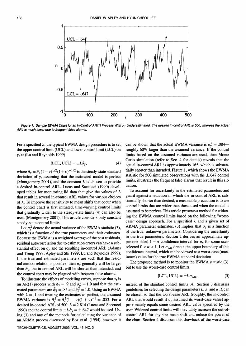
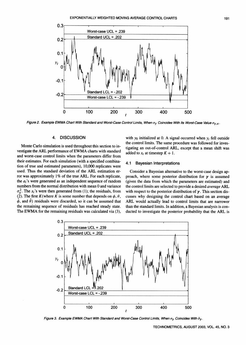
Figure 2 shows an EWMA control chart applied to 500 sim

ulated observations from the process when the true parameters assume the values (?> = .917, 9 = .491, and a2 = .102. These

parameter values were chosen because the resulting Taylor ap

proximation (7) of a2 (with V replaced by V) equals the worst

case value Gya.

One can also show that of all parameter com

binations that result in a Taylor approximation equal to cr*a,

these values have the highest likelihood (minimize yT?y y). Both the standard and the worst-case control limits are shown

in Figure 2. Because the mean of xt was held at 0 throughout the simulation, all cases where the EWMA statistic fell outside

the control limits were false alarms. The standard control lim

its resulted in false alarms around timesteps 50, 275, and 425, whereas the worst-case control limits eliminated the first two of

these. In the following section, Monte Carlo simulation is used

to provide a more comprehensive analysis of the control chart

performance.

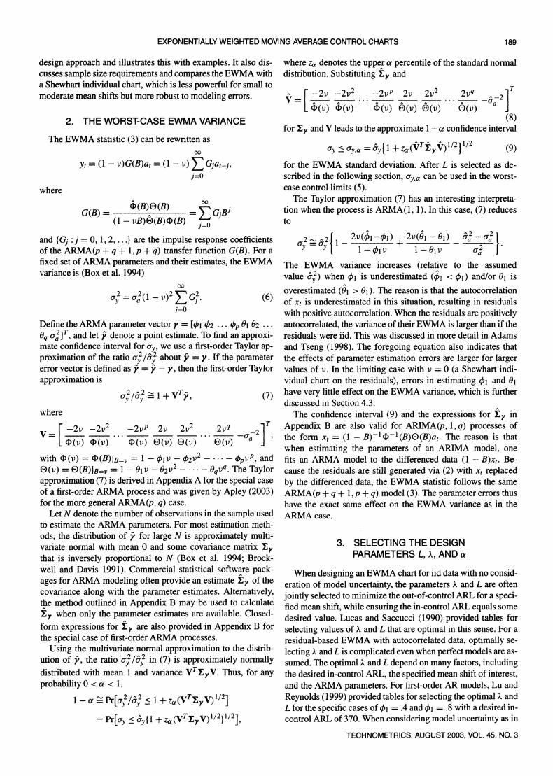
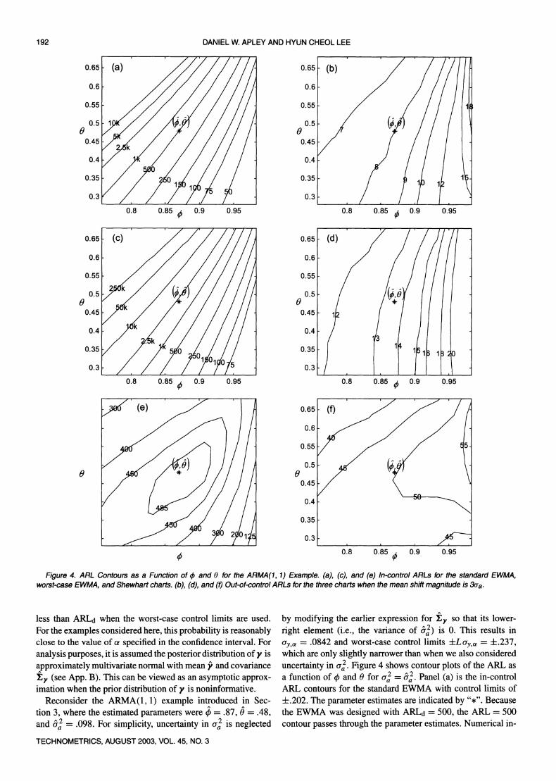
Figure 3, which is similar to Figure 2 except that the true

ARMA parameters were chosen to coincide with their esti

mates, illustrates one drawback of using the worst-case control

limits: If the true parameters happen to fall sufficiently close

to their estimates, then the standard control limits provide the

desired in-control ARL. The worst-case control limits are un

necessarily wide in this case, which inevitably decreases the

power of the control chart. This is an inherent consequence of the worst-case design approach, which is intended to guard

against the situation where the true parameters are not "suffi

ciently" close to their estimates. To mitigate this drawback, us

ing both sets of control limits for the EWMA chart is recom

mended. An observation falling outside the worst-case control

limits provides strong evidence that the process has changed. An observation falling within the worst-case control limits but

outside the standard limits should be interpreted with more cau

tion; it could mean that either the process has changed or that

the ARMA parameters differ from their estimates. Section 4

provides a detailed discussion of the trade-offs involved in the

worst-case design approach.



500

Figure 2. Example EWMA Chart With Standard and Worst-Case Control Limits, When <ry Coincides With Its Worst-Case Value oy,a.

4. DISCUSSION

Monte Carlo simulation is used throughout this section to in

vestigate the ARL performance of EWMA charts with standard

and worst-case control limits when the parameters differ from

their estimates. For each simulation (with a specified combina

tion of true and estimated parameters), 10,000 replicates were

used. Thus the standard deviation of the ARL estimation er

ror was approximately 1% of the true ARL. For each replicate, the tff's were generated as an independent sequence of random

numbers from the normal distribution with mean 0 and variance

a2. The jc/'s were then generated from (1); the residuals, from

(2). The first ?f (where K is some number that depends on 0, 0,

0, and 0) residuals were discarded, so it can be assumed that

the remaining sequence of residuals has reached steady state.

The EWMA for the remaining residuals was calculated via (3),

with yo initialized at 0. A signal occurred when yt fell outside the control limits. The same procedure was followed for inves

tigating an out-of-control ARL, except that a mean shift was

added to xt at timestep K + 1.

4.1 Bayesian Interpretations

Consider a Bayesian alternative to the worst-case design ap

proach, where some posterior distribution for y is assumed

(given the data from which the parameters are estimated) and the control limits are selected to provide a desired average ARL

with respect to the posterior distribution of y. This section dis cusses why designing the control chart based on an average

ARL would actually lead to control limits that are narrower

than the standard limits. In addition, a Bayesian analysis is con

ducted to investigate the posterior probability that the ARL is

0.3 i-,-,-,-,-1

Worst-case UCL = .239_

02 Standard UCL =

.202_,

02 Standard LCL J>.202_f_

Worst-case LCL = -.239_

_i_i_i_i_

0 100 200 300 400 500 t

Figure 3. Example EWMA Chart With Standard and Worst-Case Control Limits, When ay Coincides With ?y.



0.85 j 0.9 0.95

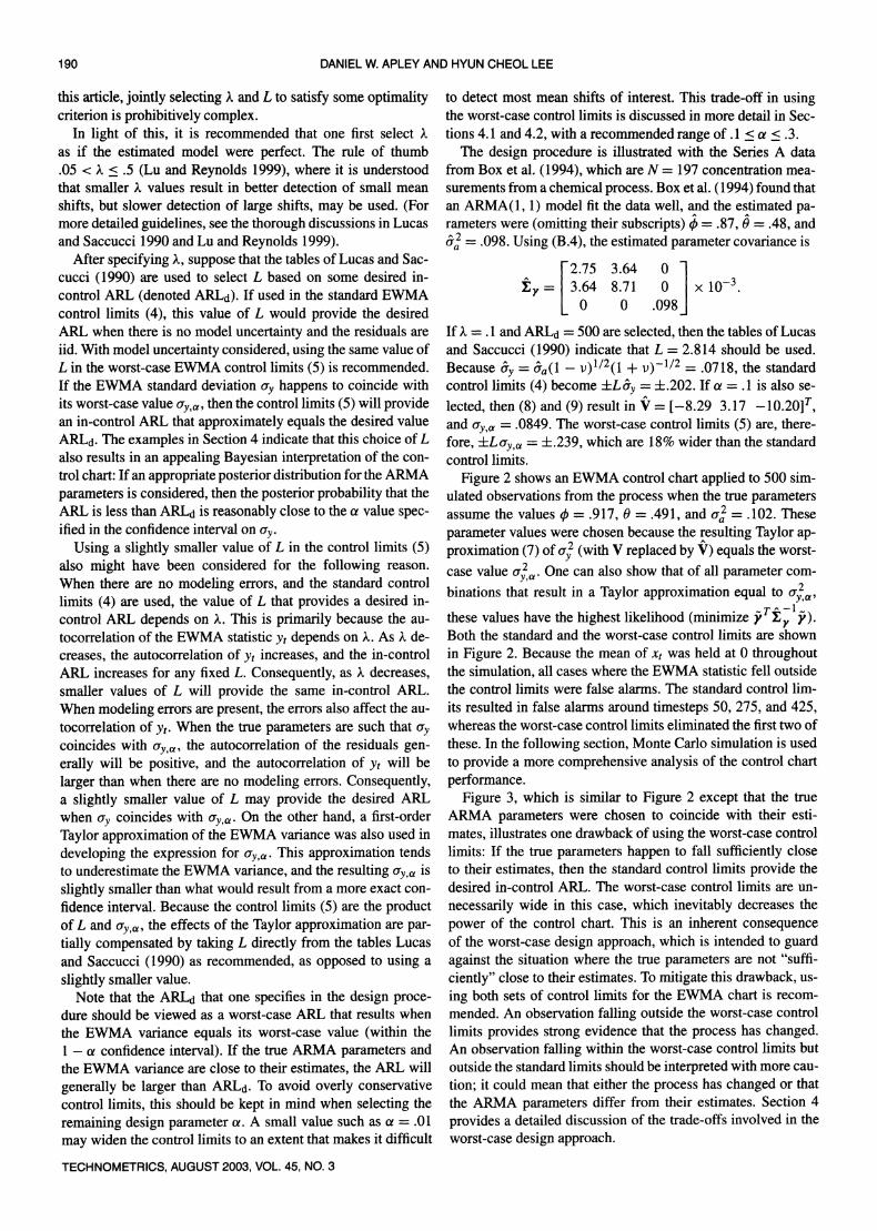
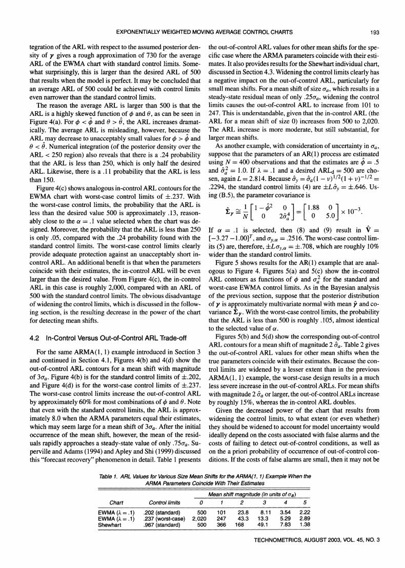
Figure 4. ARL Contours as a Function of </> and 0 for the ARMA(1,1) Example, (a), (c), and (e) ln-control ARLs for the standard EWMA, worst-case EWMA, and Shewhart charts, (b), (d), and (f) Out-of-control ARLs for the three charts when the mean shift magnitude is 3cra.

less than ARLd when the worst-case control limits are used.

For the examples considered here, this probability is reasonably close to the value of a specified in the confidence interval. For

analysis purposes, it is assumed the posterior distribution of y is

approximately multivariate normal with mean y and covariance

T?y (see App. B). This can be viewed as an asymptotic approx imation when the prior distribution of y is noninformative.

Reconsider the ARMA (1,1) example introduced in Sec

tion 3, where the estimated parameters were 0 = .87, 0 = .48, and a2 = .098. For simplicity, uncertainty in a2 is neglected

by modifying the earlier expression for ?y so that its lower

right element (i.e., the variance of o2) is 0. This results in

ay%OL = .0842 and worst-case control limits ?Loy,a

= ?.237,

which are only slightly narrower than when we also considered

uncertainty in a2. Figure 4 shows contour plots of the ARL as

a function of 0 and 0 for o2 = o2. Panel (a) is the in-control

ARL contours for the standard EWMA with control limits of

?.202. The parameter estimates are indicated by "*". Because

the EWMA was designed with ARLd = 500, the ARL = 500

contour passes through the parameter estimates. Numerical in



tegration of the ARL with respect to the assumed posterior den

sity of y gives a rough approximation of 730 for the average ARL of the EWMA chart with standard control limits. Some

what surprisingly, this is larger than the desired ARL of 500

that results when the model is perfect. It may be concluded that an average ARL of 500 could be achieved with control limits even narrower than the standard control limits.

The reason the average ARL is larger than 500 is that the

ARL is a highly skewed function of 0 and 0, as can be seen in

Figure 4(a). For 0 < 0 and 0 > 0, the ARL increases dramat

ically. The average ARL is misleading, however, because the

ARL may decrease to unacceptably small values for 0 > 0 and

0 < 0. Numerical integration (of the posterior density over the

ARL < 250 region) also reveals that there is a .24 probability that the ARL is less than 250, which is only half the desired

ARL. Likewise, there is a .11 probability that the ARL is less

than 150.

Figure 4(c) shows analogous in-control ARL contours for the

EWMA chart with worst-case control limits of ?.237. With

the worst-case control limits, the probability that the ARL is

less than the desired value 500 is approximately .13, reason

ably close to the a = . 1 value selected when the chart was de

signed. Moreover, the probability that the ARL is less than 250

is only .05, compared with the .24 probability found with the

standard control limits. The worst-case control limits clearly

provide adequate protection against an unacceptably short in

control ARL. An additional benefit is that when the parameters coincide with their estimates, the in-control ARL will be even

larger than the desired value. From Figure 4(c), the in-control

ARL in this case is roughly 2,000, compared with an ARL of

500 with the standard control limits. The obvious disadvantage of widening the control limits, which is discussed in the follow

ing section, is the resulting decrease in the power of the chart

for detecting mean shifts.

4.2 In-Control Versus Out-of-Control ARL Trade-off

For the same ARMA(1,1) example introduced in Section 3

and continued in Section 4.1, Figures 4(b) and 4(d) show the

out-of-control ARL contours for a mean shift with magnitude of 3oa. Figure 4(b) is for the standard control limits of ?.202, and Figure 4(d) is for the worst-case control limits of ?.237.

The worst-case control limits increase the out-of-control ARL

by approximately 60% for most combinations of 0 and 6. Note

that even with the standard control limits, the ARL is approx

imately 8.0 when the ARMA parameters equal their estimates, which may seem large for a mean shift of 3oa. After the initial

occurrence of the mean shift, however, the mean of the resid

uals rapidly approaches a steady-state value of only J5oa. Su

perville and Adams (1994) and Apley and Shi (1999) discussed

this "forecast recovery" phenomenon in detail. Table 1 presents

the out-of-control ARL values for other mean shifts for the spe cific case where the ARMA parameters coincide with their esti

mates. It also provides results for the Shewhart individual chart, discussed in Section 4.3. Widening the control limits clearly has a negative impact on the out-of-control ARL, particularly for small mean shifts. For a mean shift of size aa, which results in a

steady-state residual mean of only .25aa, widening the control

limits causes the out-of-control ARL to increase from 101 to

247. This is understandable, given that the in-control ARL (the ARL for a mean shift of size 0) increases from 500 to 2,020. The ARL increase is more moderate, but still substantial, for

larger mean shifts.

As another example, with consideration of uncertainty in oa,

suppose that the parameters of an AR(1) process are estimated

using N = 400 observations and that the estimates are 0 = .5

and a2 = 1.0. If X = .1 and a desired ARLd = 500 are cho

sen, again L = 2.814. Because oy =<rfl(l -

v)1/2(l + v)~1//2 =

.2294, the standard control limits (4) are ?Lay = ?.646. Us

ing (B.5), the parameter covariance is

i _,_Jl-?2 ? "I-i1"88 ?lxl0-3

**-n[ 0 2?a4J-L 0 5.0jxl? If a = .1 is selected, then (8) and (9) result in V =

[?3.27 ?

1.00]r, and ayiU = .2516. The worst-case control lim

its (5) are, therefore, ?L<xv,a = ?.708, which are roughly 10%

wider than the standard control limits.

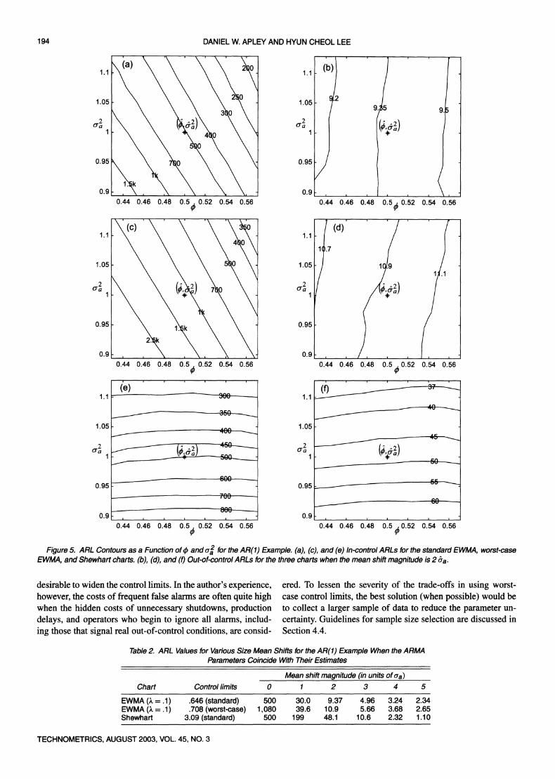
Figure 5 shows results for the AR(1) example that are anal

ogous to Figure 4. Figures 5(a) and 5(c) show the in-control

ARL contours as functions of (/> and a% for the standard and

worst-case EWMA control limits. As in the Bayesian analysis of the previous section, suppose that the posterior distribution

of y is approximately

multivariate normal with mean y and co

variance ?y. With the worst-case control limits, the probability that the ARL is less than 500 is roughly .105, almost identical

to the selected value of a.

Figures 5(b) and 5(d) show the corresponding out-of-control

ARL contours for a mean shift of magnitude 2 oa. Table 2 gives the out-of-control ARL values for other mean shifts when the

true parameters coincide with their estimates. Because the con

trol limits are widened by a lesser extent than in the previous

ARMA(1,1) example, the worst-case design results in a much

less severe increase in the out-of-control ARLs. For mean shifts

with magnitude 2 oa or larger, the out-of-control ARLs increase

by roughly 15%, whereas the in-control ARL doubles.

Given the decreased power of the chart that results from

widening the control limits, to what extent (or even whether)

they should be widened to account for model uncertainty would

ideally depend on the costs associated with false alarms and the

costs of failing to detect out-of-control conditions, as well as

on the a priori probability of occurrence of out-of-control con

ditions. If the costs of false alarms are small, then it may not be

Table 1. ARL Values for Various Size Mean Shifts for the ARMA(1, 1) Example When the ARMA Parameters Coincide With Their Estimates

Mean shift magnitude (in units of(ja)

Chart Control limits 0 12 3 4 5

EWMA(? = .1) .202 (standard) 500 101 23.8 8.11 3.54 2.22

EWMA(? = .1) .237 (worst-case) 2,020 247 43.3 13.3 5.29 2.89 Shewhart .967 (standard) 500 366 168 49.1 7.83 1.38



0.44 0.46 0.48 0.5 . 0.52 0.54 0.56 0.44 0.46 0.48 0.5/0.52 0.54 0.56

0.44 0.46 0.48 0.5 , 0.52 0.54 0.56 0.44 0.46 0.48 0.5 . 0.52 0.54 0.56

0.44 0.46 0.48 0.5 , 0.52 0.54 0.56 0.44 0.46 0.48 0.5 ,0.52 0.54 0.56

Figure 5. ARL Contours as a Function of<j> ando% for the AR(1) Example, (a), (c), and (e) In-control ARLs for the standard EWMA, worst-case

EWMA, and Shewhart charts, (b), (d), and (f) Out-of-control ARLs for the three charts when the mean shift magnitude is2aa.

desirable to widen the control limits. In the author's experience, however, the costs of frequent false alarms are often quite high when the hidden costs of unnecessary shutdowns, production

delays, and operators who begin to ignore all alarms, includ

ing those that signal real out-of-control conditions, are consid

ered. To lessen the severity of the trade-offs in using worst

case control limits, the best solution (when possible) would be

to collect a larger sample of data to reduce the parameter un

certainty. Guidelines for sample size selection are discussed in

Section 4.4.

Table 2. ARL Values for Various Size Mean Shifts for the AR(1) Example When the ARMA Parameters Coincide With Their Estimates

_Mean shift magnitude (in units of a

a)_

Chart Control limits 0 12 3 4 5

EWMA(? = .1) .646 (standard) 500 30.0 9.37 4.96 3.24 2.34 EWMA (? = .1) .708 (worst-case) 1,080 39.6 10.9 5.66 3.68 2.65 Shewhart 3.09 (standard) 500 199 48.1 10.6 2.32 1.10



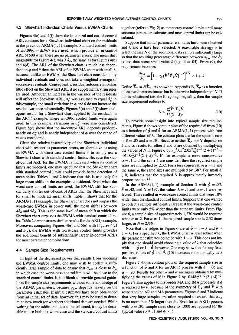
4.3 Shewhart Individual Charts Versus EWMA Charts

Figures 4(e) and 4(f) show the in-control and out-of-control

ARL contours for a Shewhart individual chart on the residuals

in the previous ARMA(1,1) example. Standard control limits

of ?3.09aa = ?.967 were used, which provide an in-control

ARL of 500 when there are no parameter errors. The mean shift

magnitude for Figure 4(f) was 3 aa, the same as for Figures 4(b) and 4(d). The ARL of the Shewhart chart is much less depen dent on (?> and 0 than the ARL of an EWMA chart with small k,

because, unlike an EWMA, the Shewhart chart considers only individual residuals and does not take a weighted average of

successive residuals. Consequently, residual autocorrelation has

little effect on the Shewhart ARL if no supplementary run rules are used. Although an increase in the variance of the residuals

will affect the Shewhart ARL, o2 was assumed to equal a2 in

this example, and small variations in (f> and 0 do not increase the

residual variance substantially. Figures 5(e) and 5(f) show anal

ogous results for a Shewhart chart applied to the residuals in

the AR(1) example, where ?3.09<j? control limits were again used. In this example, variations in o2 were also considered.

Figure 5(e) shows that the in-control ARL depends predomi

nantly on cr2 and is nearly independent of 0 over the range of

values considered.

Given the relative insensitivity of the Shewhart individual

chart with respect to parameter errors, an alternative to using an EWMA with worst-case control limits is to simply use a

Shewhart chart with standard control limits. Because the out

of-control ARL for the EWMA is increased when its control

limits are widened, one may speculate that the Shewhart chart

with standard control limits could provide better detection of

mean shifts. Tables 1 and 2 indicate that this is true only for

large mean shifts in the examples considered. Even when the

worst-case control limits are used, the EWMA still has sub

stantially shorter out-of-control ARLs than the Shewhart chart

for small to moderate mean shifts. Table 1 shows that for the

ARMA(1,1) example, the Shewhart chart does not surpass the

worst-case EWMA in power until the mean shift is between

4aa and 5aa. This is the same level of mean shift at which the

Shewhart chart surpasses the EWMA with standard control lim

its. Table 2 demonstrates similar results for the AR(1) example. Moreover, comparing Figures 4(e) and 5(e) with Figures 4(c) and 5(c), the EWMA with worst-case control limits provides the additional benefit of substantially larger in-control ARLs

for most parameter combinations.

4.4 Sample Size Requirements

In light of the decreased power that results from widening the EWMA control limits, one may wish to collect a suffi

ciently large sample of data to ensure that ay# is close to ay, in which case the worst-case control limits will be close to the

standard control limits. It is difficult to provide general guide lines for sample size requirements without some knowledge of

the ARMA parameters, because oy,a depends heavily on the

parameter estimates. If initial estimates have been obtaineded

from an initial set of data, however, this may be used to deter

mine how much (or whether) additional data are needed. While

waiting for the additional data to be collected, it may be desir

able to use both the worst-case and the standard control limits

together (refer to Fig. 2) as temporary control limits until more

accurate parameter estimates and new control limits can be cal

culated.

Suppose that initial parameter estimates have been obtained

and k and a have been selected. A reasonable strategy is to

select the size N of the additional data sample sufficiently large so that the resulting percentage difference between oy,a and oy is less than some small value 8 (e.g., 8 = .05). From (9), the

requirement becomes

a-^ =

[l+Za(\T?yvf2]l/2<l+8. Define T.y

= NT,y. As shown in Appendix B, Hy is a function

of the parameter estimates but is otherwise independent of N. If

this is substituted into the foregoing inequality, then the sample size requirement reduces to

z2yT~? y

K>t??W>- (10>

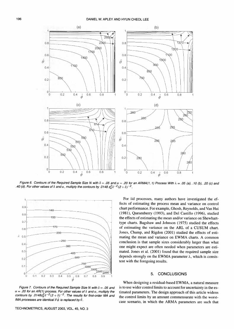
To provide some insight into typical sample size require ments, Figure 6 shows contour plots of the required N from (10) as a function of 0 and 0 for an ARMA(1,1) process with four

different values of k. The contour plots are for the specific case

of 8 = .05 and a = .20. Because neither Ey nor V depends on

8 and a, results for other 8 and a are obtained by multiplying the values of N in Figure 6 by z^2.0522.052z2<r2(2 + 8)~2 =

.0148z2<5~2(2 + 8)~~2. If, for example, a more conservative a = . 1 and the same <5 are consider, then the required sample sizes are multiplied by 2.32. For a less conservative a = .3 and

the same 8, the same sizes are multiplied by .387. For small 8,

(10) indicates that the required N is approximately inversely

proportional to 82. In the ARMA(1,1) example of Section 3 with 0 = .87,

0 = .48, and N = 197, the values k = .1 and a = .1 were se

lected. This resulted in worst-case control limits that were 18%

wider than the standard control limits. Suppose that one wanted

to collect a sample sufficiently large that the worst-case control

limits were only 5% wider than the standard limits. From Fig ure 6, a sample size of approximately 1,270 would be required when a = .2. For a = . 1, the required sample size is 2.32 times

larger, orN = 2,940. Note that the ridges in Figure 6 are at 0 = 1 ? k and 0 =

1 ? k. For a specified k, the EWMA chart is least robust when

the parameter estimates coincide with 1 ? k. This does not im

ply that one should avoid choosing a value of k that coincides

with 1 ? 0 or 1 ?

0, however. One may show that for any fixed

positive values of 0 and 9, (10) increases monotonically as k

decreases.

Figure 7 shows contour plots of the required sample size as

a function of 0 and k for an AR(1) process with 8 = .05 and

a = .20. Results for other 8 and a are again obtained by mul

tiplying the values of N in Figure 7 by .0148z2<$~2(2 + 8)~2.

Figure 7 also applies to first-order MA and IMA processes if 0 is replaced by 0, because of the symmetry of T,y and V with

respect to the AR and MA parameters. Figures 6 and 7 indicate

that very large samples are often required to ensure that oy,a is no more than 5% larger than oy. Even for an AR(1) process

with a = .20, sample sizes close to 1,000 are required for the

typical values ?^.l and 0 > .5.



(a) (b)

0.8 _______J~~ ^^^^^^ii 0.8

:-__~^

0 0.2 0.4 ; 0.6 0.8 1 0 0.2 0.4 ; 0.6 0.8 1 <P <P

(c) (d)

0.8 - _??^f J^3

?-8 -?^^^ ) \ 2^v

0.6 -?___^~^^~"-^. \" \\( (ft

0.6 "

:

0 0.2 0.4 ; 0.6 0.8 1 0 0.2 0.4 ; 0.6 0.8 1

Figure 6. Contours of the Required Sample Size N with 8 = .05 and a = .20 for an ARMA(1, 1) Process With X = .05 (a), . 10 (b), .20 (c) and

.40 (d). For other values of 8 anda, multiply the contours by .0148 z?8~2(2 + 8)~2.

1 i-1-1-1-1-1-1-1-1-r

Figure 7. Contours of the Required Sample Size N with 8 = .05 and a = .20 for an AR(1) process. For other values of 8 anda, multiply the

contours by .0148z?8~2(2 + 8)~2. The results for first-order MA and

IMA processes are identical if(?> is replaced by 6.

For iid processes, many authors have investigated the ef fects of estimating the process mean and variance on control chart performance. For example, Ghosh, Reynolds, and Van Hui

(1981), Quesenberry (1993), and Del Castillo (1996), studied the effects of estimating the mean and/or variance on Shewhart

type charts. Bagshaw and Johnson (1975) studied the effects of estimating the variance on the ARL of a CUSUM chart.

Jones, Champ, and Rigdon (2001) studied the effects of esti

mating the mean and variance on EWMA charts. A common

conclusion is that sample sizes considerably larger than what one might expect are often needed when parameters are esti

mated. Jones et al. (2001) found that the required sample size

depends strongly on the EWMA parameter k, which is consis tent with the foregoing results.

5. CONCLUSIONS

When designing a residual-based EWMA, a natural measure is to use wider control limits to account for uncertainty in the es timated parameters. The design approach of this article widens the control limits by an amount commensurate with the worst case scenario, in which the ARMA parameters are such that



the EWMA variance equals the maximum value within an ap

propriate confidence interval. Assuming that an estimate of the

parameter covariance matrix is available or can be calculated as described in Appendix B, the worst-case design approach involves little additional complexity relative to the standard de

sign approach. In light of the drawback of widening the control limits?

decreased chart power?one may question whether residual

based control charts should be used. The impact of parame ter uncertainty, however, is not unique to residual-based charts.

Suppose that a CUSUM, X, or EWMA chart is to be applied

directly to an autocorrelated process xt. The methods presented

by Johnson and Bagshaw (1974), Vasilopoulos and Stamboulis

(1978), and Zhang (1998) rely on an accurate ARMA process model (or, equivalently, the autocorrelation function of xt) just as residual-based control charts do. The difference is that in

residual-based control charts, the charted statistic depends on

the model, whereas the control limits do not. In control charts

applied directly to xt, the control limits depend on the model, whereas the charted statistic does not. If the estimated model

is inaccurate in either case, then the control limits will fail to

provide the desired ARL.

Noting the lack of robustness of residual-based charts to pa rameter errors, Adams and Tseng (1998) recommended the al

ternative approach of removing (when possible) the autocorre

lation by either removing the source or using feedback-control

techniques. Effective removal of autocorrelation via feedback

control also requires an accurate process model, however. With

modeling errors, the feedback-controlled process output would

have autocorrelation similar to the ARMA residuals. A con

trol chart on the output would most likely be just as affected

by modeling errors as a control chart on the residuals. An in

vestigation of the relative robustness of different control charts

(on the residuals, on xt, and on the feedback-controlled output) would shed light on whether there are any significant differ

ences in their sensitivity to modeling errors.

ACKNOWLEDGMENTS

The editor, the associate editor, and an anonymous referee

have made numerous helpful comments that greatly improved the quality of this article. This work was supported by the State

of Texas Advanced Technology Program grant 000512-0289

1999 and the National Science Foundation grant DMI-0093580.

APPENDIX A: DERIVATION OF THE FIRST-ORDER TAYLOR APPROXIMATION (7) FOR

ARMA(1,1) PROCESSES

The first-order Taylor approximation of the ratio

a* a02(l-v2)fr2

a2 a2 ?-^ J y a

y=o

is sought, where (6) has been used for or2. The approximation is

r = r\y=v +

8r

+ dr

3?f

y=y OU

(?2

(?-e) y=y

iK-??) y=y

= 1+2(1-v2)?(g,.?)| *

;--0V Wt\y=y 7=0

A ~2

(A.1)

For ARMA(1,1) processes, G(B) can be expressed via its par tial fraction expansion

G(B) = (l-0g)(l -6>_?)

(l-v_?)(l-o_0(l-</_?)

(v-<t>)(v-9) 1 +

(<p-(t>)(<i>-e) i

(v -

6?)(v -

0) (1 -

vB) (</, _

?)(0 _

6?) (1 -

0B)

+ (0_-0)(0-0) 1

(0 -

v)(9 -

(?>) (I -

OB)

which can be verified by straightforward but tedious algebra. For notational convenience, the subscripts on

<f> and 6 have

been omitted. Because (1 ?

cB)~x = Ylj^o0'^

f?r any con"

stant c with magnitude less than unity, the impulse response coefficients are

(v-4>){v-e) j t (<t>-$)(<p-9)^ Gj =-x-vJ H-?<p>

iv-e){v-4>) {<t>-v){4>-e)

H-x-x-fr.

Hence

(e-v)(?-4>)

Gj\y=y=vK

-E^l4+> y=y J=o

1

V ?0 V ? 0

1 1

;=0 y=y j=0

V ? (?> \\

? 4>V 1 ? V2

? V

(l-</>v)(l-v2)'

-0 v-0

1 1

and

E^ 7=0

v-0[l-v2 l-0v V

(l-0v)(l-v2)'

00 -

f-' 1-V2 ?=y 7=0

Substituting these into (A.l) gives (7).



APPENDIX B: CALCULATING THE PARAMETER COVARIANCE X,

Assume that the ARMA parameters are estimated using a

method based on minimizing the sum of the squares of the model residuals, such as the nonlinear least squares or approx imate maximum likelihood methods described by Box et al.

(1994). For sample size N sufficiently large, the parameter co

variance matrix is (Box et al. 1994)

L,y -

0T

0

2AT l?i

i

?

-l

0T

0

2ai (B.l)

where 0 denotes a column vector of p + q Os, and J,n denotes

the covariance of r? = [0i 02 ... <?>p 0\ 02 0q]T. The matrix

?w is defined as the covariance matrix of the random vector

w, = [ut ut-\ ...

?i-p+i vt vt-\ ... vt-q+\]T,

where ut and vt

are defined via ut ?

<t>~l(B)at and vt = ?S~l(B)at.

To calculate Xw, rewrite ut = J2hLo8<t>Jat-j and Vt =

- Yj^o8ojaH>

wnere the ?0,/s and go/s are the impulse re

sponse coefficients of <t>~l(B) and S~l(B). Note that the im

pulse response coefficients can be calculated recursively for

j= 1,2,..., via

g4>J =

0i?0J-i + 02?0?-2 + * ' + 4>p84>J-p> (B-2)

and

gej =

Oigej-i + 02gej-2 + + 0qg9J-q (B.3)

with gjj =

g6>j = 0 for./ < 0 and ?<?,o

= ?0,0 = 1. If the matrix

H=

" ?0,0 0

<?0,i ?0,0

?0,2 ?0,1

?0,p ?0,p-l

?0,p+l ?0,p

0

0

?0,0

?0,1

?0,2

-go,o

-?0,2

'>e,q

0

-?0,0

-?0,1

-8e,q

0

0

~8e,o

-?0,1

-?0,2

is constructed from the impulse response coefficients, then

Iw = cr2HrH results, and crfa~l = [HrH]-1 can be substi

tuted in (B.l). Because the impulse response coefficients decay

exponentially for stable, invertible ARMA processes, the num

ber of rows needed in H will generally be reasonable.

Because the true ARMA parameters are unknown, their esti

mates must be substituted into (B.1)-(B.3) to calculate the esti

mate Y,y for use in the confidence interval (9). Box et al. (1994) showed that for first-order AR, MA, and ARMA processes, the

estimated covariance of r? reduces to the following:

ARMA(1,1): I,= (1-00)

N(4>-?)2

Rl-02)(l-00) (1-02)(1-02)1 L(l-02)(l-02) (1-02)(1-00)J'

(B.4)

AR(1): If = 1-02

N (B.5)

and

MA(1): ?f = I

[Received April 2000. Revised March 2003.]

REFERENCES

Adams, B. M., and Tseng, I. T. (1998), "Robustness of Forecast-Based Moni

toring Schemes," Journal of Quality Technology, 30, 328-339.

Alwan, L. C, and Roberts, H. V. (1988), 'Time-Series Modeling for Statistical Process Control," Journal of Business and Economic Statistics, 6, 87-95.

Apley, D. W. (2003), 'The Sensitivity of EWMA Charts for Autocorrelated

Processes," Technical Report 2003-001, Texas A&M University, Dept. of In dustrial Engineering.

Apley, D. W., and Shi, J. (1999), "The GLRT for Statistical Process Control of

Autocorrelated Processes," HE Transactions, 31,1123-1134.

Bagshaw, M., and Johnson, R. A. (1975), "The Influence of Reference Values and Estimated Variance on the ARL of CUSUM Tests," Journal of the Royal Statistical Society, Ser. B, 37,413-420.

Berthouex, P. M., Hunter, W. G., and Pallesen, L. (1978), "Monitoring Sewage Treatment Plants: Some Quality Control Aspects," Journal of Quality Tech

nology, 10, 139-149.

Box, G., Jenkins, G., and Reinsei, G. (1994), Time Series Analysis, Forecasting, and Control (3rd ed.), Englewood Cliffs, NJ: Prentice-Hall.

Brockwell, P. J., and Davis, R. A. (1991), Time Series: Theory and Methods

(2nd ed.), New York: Springer-Verlag. _ Del Castillo, E. (1996), "Evaluation of Run Length Distribution for X Charts

With Unknown Variance," Journal of Quality Technology, 28, 116-122.

English, J. R., Krishnamurthi, M., and Sastri, T. (1991), "Quality Monitoring of Continuous Flow Processes," Computers and Industrial Engineering, 20, 251-260.

Ghosh, B. K., Reynolds, M. R., and Van Hui, Y. V. (1981), "Shewhart X-Charts

With Estimated Process Variance," Communications in Statistics: Theory and

Methods, 18, 1797-1822.

Johnson, R. A., and Bagshaw, M. (1974), 'The Effect of Serial Correlation on

the Performance of CUSUM Tests," Technometrics, 16, 103-112.

Jones, L. A., Champ, C. W., and Rigdon, S. E. (2001), "The Performance of Ex

ponentially Weighted Moving Average Charts With Estimated Parameters,"

Technometrics, 43, 156-167.

Lin, W. S., and Adams, B. M. (1996), "Combined Control Charts for Forecast

Based Monitoring Schemes," Journal of Quality Technology, 28, 289-301.

Lu, C. W., and Reynolds, M. R. (1999), "EWMA Control Charts for Monitoring the Mean of Autocorrelated Processes," Journal of Quality Technology, 31, 166-188.

Lucas, J. M., and Saccucci, M. S. (1990), "Exponentially Weighted Moving

Average Control Schemes: Properties and Enhancements," Technometrics,

32, 1-12.

Montgomery, D. C. (2001), Introduction to Statistical Quality Control (4rd ed.), New York: Wiley.

Montgomery, D. C, and Mastrangelo, C. M. (1991), "Some Statistical Process

Control Methods for Autocorrelated Data," Journal of Quality Technology, 23,179-193.

Montgomery, D. C, and Woodall, W. H. (1997), "A Discussion on Statistically Based Process Monitoring and Control," Journal of Quality Technology, 29, 121-162.

Quesenberry, C. P. (1993), 'The Effect of Sample Size on Estimated Limits for

X and X Control Charts," Journal of Quality Technology, 25, 237-247.

Runger G. C, Willemain, T. R., and Prabhu, S. (1995), "Average Run Lengths for Cusum Control Charts Applied to Residuals," Communications in Statis

tics: Theory and Methods, 24, 273-282.

Superville, C. R., and Adams, B. M. (1994), "An Evaluation of Forecast-Based

Quality Control Schemes," Communications in Statistics: Simulation and

Computation, 23, 645-661.

Vander Wiel, S. A. (1996), "Monitoring Processes That Wander Using Inte

grated Moving Average Models," Technometrics, 38, 139-151.

Vasilopoulos, A. V., and Stamboulis, A. P. (1978), "Modification of Control

Chart Limits in the Presence of Data Correlation," Journal of Quality Tech

nology, 10, 20-30.

Wardell, D. G., Moskowitz, H., and Plante, R. D. (1994), "Run-Length Distri

butions of Special-Cause Control Charts for Correlated Processes," Techno

metrics, 36, 3-17.

Zhang, N. F. (1998), "A Statistical Control Chart for Stationary Process Data,"

Technometrics, 40, 24-38.


design of exponentially weighted moving average control...

Documents