A New Exponentially Weighted Moving

Average Control Chart for Monitoring the

Coefficient of Variation

Jiujun Zhang a, Zhonghua Li b, Bin Chen c, Zhaojun Wang b,∗aDepartment of Mathematics, Liaoning University, Shenyang 110036, P.R.ChinabLPMC and Institute of Statistics, Nankai University, Tianjin 300071, P.R.China

cSchool of Mathematics and Statistics, Jiangsu Normal University, Xuzhou221116, P.R.China

Abstract

Monitoring coefficient of variation is one of the successful approaches to StatisticalProcess Control (SPC) when the process mean and standard deviation are notconstants. This paper presents a modified Exponentially Weighted Moving Average(EWMA) chart in order to further enhance the sensitivity of the EWMA controlchart proposed by Castagliola et al. (2011). Tables are provided for the statisticalproperties of the new chart. Some numerical results and comparisons are given andshow that the new chart has an average run length performance that is superior tosome other competing procedures. A real data example from manufacturing showsthat it performs quite well in applications.

Key words: Coefficient of Variation; Exponentially Weighted Moving Average;Average Run Length; Statistical Process Control1991 MSC: 62P30

1 Introduction

Ever since Shewhart introduced control charts, it has become a common prac-tice for practitioners to use various control charts to monitor different pro-

∗ Corresponding author.Email addresses: zjjly790816@163.com (Jiujun Zhang), zli@nankai.edu.cn

(Zhonghua Li), bchen@jsnu.edu.cn (Bin Chen), zjwang@nankai.edu.cn Tel:

86-22-23498233 Fax: 86-22-23506423 (Zhaojun Wang).

Preprint submitted to Computers & Industrial Engineering 17 October 2014

cesses. When we deal with variable data, the charting technique usually em-ploys a chart to monitor the process mean and another chart to monitor theprocess variance. The Shewhart �̄� and 𝑆 (or 𝑅) charts are industry standardsfor quality control applications where the mean 𝜇 and the standard deviation𝜎 of a process must be statistically controlled at the nominal values 𝜇0 and𝜎0. The baseline assumption is that the nominal values are fixed constants,and there are indeed many applications for which this assumption is reason-able. To this end, it is reasonable to monitor the process mean and variancesimultaneously by a single chart, see Zhang et al. (2010, 2011), Costa et al.(2013), Du et al. (2013) and Menzefricke (2013a,b). However, control chartingtechniques were recently extended to various service sectors such as health,education, finance (see Sharpe, 1994) and various societal applications. In ad-dition, it is also adopted in chemical and biological assay quality control tovalidate results, where the mean and the standard deviation may not be con-stants all the time and the process may nevertheless be declared in-controlif their ratio remains stable around a constant value, see Reed et al. (2002).As stated by Castagliola et al. (2013a,b), there are many opportunities forSPC monitoring of the coefficient of variation (CV) also in the fields of mate-rials engineering and manufacturing. Tool cutting life and several propertiesof sintered materials are typical examples from this setting, and hence we willshow our proposed scheme performs quite well in applications through a realdata example from sintered materials manufacturing. In this case, the routineuse of the Shewhart charts is dubious, even though statistical control is stillsought. For example, direct proportionality 𝜎 = 𝛾𝜇 is a common relationshipbetween the mean and standard deviation in some processes. In this less re-strictive setting, 𝜇 and 𝜎 may vary in the parameter space subject only to𝛾 = 𝜎

𝜇, so that only the CV parameter, 𝛾 , is constant. In this case, it is nat-

ural to explore the use of the CV. Several published works have investigatedthe distribution of sample CV and its related inferential properties, see Hen-dricks and Robey (1996), Iglewicz et al. (1968), Mckay (1932), Mahmoudvandand Hassani (2009), Reh and Scheffler (1996), Tian (2005), Vangel (1996) andVerrill and Johnson (2007).

Recently, Kang et al. (2007) developed a Shewhart-Type control chart formonitoring the cyclosporine level in organ-transplantation procedures usingrational subgroups. As stated by Kang et al. (2007), the advantage of adopting𝛾 as the monitored statistic by a control chart is evident for those chemical orphysical processes for which the variation of a quality characteristic 𝑋 has tobe controlled and the population standard deviation 𝜎 is proportional to themean 𝜇. This Shewhart-Type chart is sensitive to large shifts but not sensitiveto small to moderate shifts. The EWMA chart is also a good alternative to theShewhart control chart when we are interested in detecting small shifts. Theperformance of the EWMA control chart is approximately equivalent to thatof the cumulative sum (CUSUM) control chart, and in some ways it is easierto set up and operate. To this end, Hong et al. (2008) proposed an EWMA-CV

2

control chart in order to improve the Shewhart-type chart proposed by Kanget al. (2007) and detect small shifts more efficiently.

Castagliola et al. (2011) suggested a new method to monitor the CV by meansof two one-sided EWMA charts of the CV squared. A numerical analysisdemonstrated that this chart almost always performed better than the controlchart proposed by Hong et al. (2008) even if this statistical outperformance isoften rather small. However, the authors did not investigate the simultaneousmonitoring of increasing or decreasing shifts in CV, which is important in realapplications.

Recently, Calzada and Scariano (2013) developed a synthetic control chart formonitoring the CV. The results showed that the synthetic chart performedbetter than that of Kang et al. (2007), but worse than Castagliola et al. (2011)as long as the increasing shift in the CV is not too large. In addition, Castagli-ola et al. (2013a) evaluated an adaptive Shewhart control chart implementingvariable sampling interval strategy to monitor the process CV. Castagliola etal. (2013b) proposed a Shewhart chart with supplementary run rules to moni-tor the CV. However, as they pointed out, the run rules charts for monitoringthe CV does not outperform more advanced strategies like the chart proposedby Castagliola et al. (2011) or the synthetic chart proposed by Calzada andScariano (2013).

The goal of this paper is to improve the performance of EWMA−𝛾2 chartbased on the preliminary work of Castagliola et al. (2011) by proposing anew strategy for monitoring the coefficient of variation. The remainder ofthis paper is organized as follows. A brief review of the one-sided EWMA−𝛾2

chart of Castagliola et al. (2011) is given in Section 2. Following that, ourmodified EWMA chart is presented and the statistical performance of thenew chart is investigated. Sets of optimal design parameters are also providedfor different values of the in-control coefficient of variation, for different samplesizes, and for a wide range of deterministic shifts, including both decreasingand increasing cases in this Section. The numerical comparisons with someother procedures are carried out in Section 3. The application of our proposedmethod is illustrated in Section 4 by a real data example from chemical processcontrol. Several remarks conclude this paper in Section 5.

Now we summarize some abbreviated expressions used in this paper for easyreference and recapitulation.

∙ EWMA: exponentially weighted moving average; Cusum: cumulative sum.∙ CV: coefficient of variation;MCV: modified chart for monitoring CV (this paper proposed);ECV: EWMA chart for monitoring CV (Castagliola et al. ,2011);SynCV: synthetic chart for monitoring CV (Calzada and Scariano, 2013);

3

SRCV: Shewhart chart with supplementary run rules for monitoring CV(Castagliola et al., 2013b);

∙ UCL: upper control limit; LCL: lower control limit; UWL: upper warninglimit; LWL: lower warning limit;

∙ IC: in-control; OC: out-of-control;∙ ARL: average run length; ZS-ARL: zero-state average run length;SDRL: standard deviation of the run length.

2 Monitoring CV with new modified EWMA chart

Suppose that we observe subgroups 𝑋𝑘1, 𝑋𝑘2, ⋅ ⋅ ⋅ , 𝑋𝑘𝑛 of size n at times 𝑘 =1, 2, ⋅ ⋅ ⋅. We also assume that there is independence within and between thesesubgroups and each random variable 𝑋𝑘𝑗 follows a normal 𝑁(𝜇𝑘, 𝜎𝑘) distribu-tion, where parameters 𝜇𝑘 and 𝜎𝑘 are constrained by the relation 𝛾𝑘 =

𝜇𝑘

𝜎𝑘= 𝛾0

when the process is in control. This implies that, from one subgroup to an-other, the values of 𝜇𝑘 and 𝜎𝑘 may change, but the coefficient of variation𝛾𝑘 = 𝜇𝑘

𝜎𝑘must be equal to some predefined in-control value 𝛾0, common to all

the subgroups.

2.1 A brief review of EWMA−𝛾2 chart (Castagliola et al., 2011)

In this subsection, we give a brief review of the EWMA−𝛾2 chart proposed byCastagliola et al.(2011) (denoted as ECV chart). First, an upward ECV chartaims to detect an increase in the CV and is defined as

𝑍+𝑘 = max(𝜇0(𝛾

2), (1− 𝜆+)𝑍+𝑘−1 + 𝜆+𝛾𝑘

2), (1)

with 𝑍+0 = 𝜇0(𝛾

2) as the initial value and with the asymptotic correspondingupper control limit (UCL)

𝑈𝐶𝐿 = 𝜇0(𝛾2) +𝐾+

√𝜆+

2− 𝜆+𝜎0(𝛾2). (2)

Second, a downward ECV chart aims to detect a decrease in the CV and isdefined as

𝑍−𝑘 = min(𝜇0(𝛾

2), (1− 𝜆−)𝑍−𝑘−1 + 𝜆−𝛾𝑘

2), (3)

with 𝑍−0 = 𝜇0(𝛾

2) and with the asymptotic corresponding lower control limit(LCL)

4

𝐿𝐶𝐿 = 𝜇0(𝛾2) +𝐾−

√𝜆−

2− 𝜆−𝜎0(𝛾2), (4)

where 𝜇0(�̂�2) and 𝜎0(�̂�

2) are the mean and standard deviation of 𝛾2 when theprocess is in control and 𝜆+(𝜆−) and 𝐾+(𝐾−) are the smoothing constant andchart coefficient of the upward (downward) ECV chart. Approximations for𝜇0(�̂�

2) and 𝜎0(�̂�2) are provided by Breunig (2001) as

𝜇0(𝛾2) = 𝛾2

0(1−3𝛾2

0

𝑛), (5)

and

𝜎0(𝛾2) = {𝛾4

0(2

𝑛− 1+ 𝛾2

0(4

𝑛+

20

𝑛(𝑛− 1)+

75𝛾20

𝑛2))− (𝜇0(�̂�

2)− 𝛾20)

2} 12 . (6)

The suggested one-sided EWMA charts have many advantages according toCastagliola et al. (2011). However, it should be noted that, in Equation (1),when 𝜇0(𝛾

2) > (1− 𝜆+)𝑍+𝑘−1 + 𝜆+𝛾𝑘

2, then 𝑍+𝑘 = 𝜇0(𝛾

2). So, in the next timepoint, we have

𝑍+𝑘+1 = max(𝜇0(𝛾

2), (1− 𝜆+)𝜇0(𝛾2) + 𝜆+𝛾2

𝑘+1). (7)

It is obvious that the samples collected before time 𝑘 + 1 are not used anylonger. However, the advantage of the EWMA chart is that it will use not onlythe information of the current sample but also will use the former samples.To this end, in order to improve the performance of the ECV chart, next, wepropose a modified EWMA chart based on the ECV chart. The comparisonresults showed that the new chart performs much better than the ECV chart,especially for detecting small to moderate shifts in CV.

2.2 Our modified methodology

To further enhance the sensitivity of the ECV chart in monitoring the processCV, we propose a modified procedure to the construction of 𝑍+

𝑘 and 𝑍−𝑘 . First,

we define a new upward EWMA chart based on the sample CV (denoted asupward MCV chart), 𝛾𝑘

2, as follows:

𝑍+𝑘 = max(𝜇0(𝛾

2), 𝑈+𝑘 ), (8)

where 𝑈+𝑘 is defined as

5

𝑈+𝑘 = (1− 𝜆+)𝑈𝑘−1 + 𝜆+𝛾𝑘

2, (9)

where 𝑈+0 = 𝜇0(𝛾

2) as the initial value. The asymptotic corresponding UCL isthe same as defined in Equation (2). Note that the difference between the MCVand the ECV charts is that our new chart will use not only the informationof the current sample but also will use all of the former samples. So, it isexpected that the new chart will be more effective than the ECV chart.

Second, a new downward EWMA chart based on the sample CV (denoted asdownward MCV chart), 𝛾𝑘

2, as follows:

𝑍−𝑘 = max(𝜇0(𝛾

2), 𝑈−𝑘 ), (10)

where 𝑈−𝑘 is defined as

𝑈−𝑘 = (1− 𝜆−)𝑈𝑘−1 + 𝜆−𝛾𝑘

2, (11)

where 𝑈−0 = 𝜇0(𝛾

2) as the initial value. The asymptotic corresponding LCL isthe same as defined in Equation (4).

An alarm is triggered as soon as 𝑍+𝑘 > 𝑈𝐶𝐿 or 𝑍−

𝑘 < 𝐿𝐶𝐿, respectively. Acombination of the two one-sided charts can be implemented to detect bothincrease and decrease shifts in CV. The 𝐾 values of the upper and lowercharts for some combinations of 𝜆, 𝛾0 and 𝑛 are presented in Tables 1-2 whenthe in control average run length (IC-ARL) is 370. Upon request, Fortranprograms that optimize our new CV chart for other parameter conditions willbe provided.

3 Numerical results and comparison

In this paper, the average run length (ARL) measures the efficiency of a con-trol chart in detecting a process change. This ARL performance is usuallyreferred to as the zero-state ARL(ZS-ARL) performance.When the processis in control, it is desirable that the expected number of samples, in-controlARL(IC-ARL), taken since the beginning of the monitoring until a signal islarge, to guarantee few false alarms. When the process is out of control, it isdesirable that the expected number of samples, out-of-control ARL(OC-ARL),taken since the occurrence of the assignable cause until a signal is small, inorder to guarantee fast detection of process changes. A control chart is con-sidered better than its competitors if it has the smaller OC-ARL value for aspecific shift 𝜏 ∗ in CV when IC-ARL is the same for all the charts. In thissection, the performance of our new chart is compared with some competing

6

charts, including the ECV chart, the synthetic CV chart and the Shewhartchart with supplementary run rules, respectively.

3.1 ARL optimization for the new chart and the comparison with ECV chart

Assume that when the process is in-control, 𝛾 = 𝛾0 and when the process isout-of-control, 𝛾 = 𝛾1 = 𝜏𝛾0. Values of 0 < 𝜏 < 1 correspond to a decreaseof the nominal coefficient of variation, while values of 𝜏 > 1 correspond to anincrease of the nominal coefficient of variation. An optimization philosophywill be considered in this study. In the standard optimization procedure, twospecial ARL cases merit special attention: the in-control case IC-ARL andout-of-control case OC-ARL, for specified 𝛾1. Once consideration is given tothe cost of halting a stable process to investigate a false-alarm signal, thechart designer specifies IC-ARL at an acceptable level. Next, considerationis given to the magnitude of a shift in the CV, 𝛾 = 𝜏𝛾0, regarded as mostdetrimental to process quality, which must be identified and eliminated assoon as possible. An optimal modified CV chart would minimize the ARL atthis shift, 𝜏 ∗, subject to the chosen in-control ARL constraint. That is, optimalvalues (𝜆∗, 𝐾∗) are given by

(𝜆∗, 𝐾∗) = arg min(𝜆,𝐾)

𝐴𝑅𝐿(𝛾0, 𝛾1, 𝜆,𝐾, 𝑛), (12)

subject to the constraint

𝐴𝑅𝐿(𝛾0, 𝛾0, 𝜆∗, 𝐾∗, 𝑛) = 𝐴𝑅𝐿0. (13)

Similar to Castagliola et al.(2011), the complete heuristic design procedure isimplemented as follows:

– when the process is functioning at the nominal coefficient of variation 𝛾 = 𝛾0,then 𝐴𝑅𝐿 = 𝐴𝑅𝐿0, where 𝐴𝑅𝐿0 is some predefined IC-ARL value.

– for a specified value 𝛾 = 𝜏 ∗𝛾0 ∕= 𝛾0, the couple (𝜆∗, 𝐾∗) yields the smallestpossible OC-ARL.

We compare our new chart with ECV chart in terms of the OC-ARL. TheECV chart introduced by Castagliola et al.(2011) is statistically more efficientat detecting small process shifts than the regular Shewhart control chart. Forfair comparisons, the values of 𝜆∗ is always kept larger than 0.05 in order to beconsistent with Castagliola et al.(2011). Tables 3 and 4 compare selected OC-ARLs for the one-sided ECV chart and the new chart, where all charts havean IC-ARL of 370 and have been optimized to minimize OC-ARLs at shift 𝜏 ∗.

7

The optimal couples (𝜆∗, 𝐾∗) for the new charts are presented in the first rowof each block of Tables 3 and 4, for 𝑛 = {5, 7, 10, 15}, 𝛾0 = {0.05, 0.1, 0.15, 0.2},and 𝜏 ∗ = {0.5, 0.65, 0.8, 0.9} (i.e. decreasing case), 𝜏 ∗ = {1.1, 1.25, 1.5, 2.} (i.e.increasing case), while the out-of-control ZS-ARLs of the MCV(left side) andECV (right side) charts are presented in the second row of each block. Ingeneral, the run length distribution of a control chart can be explored byintegral equations, Markov Chain or by a Monte Carlo simulation (Li et al,2014). In this study, we used the Monte Carlo simulation approach throughan algorithm developed in FORTRAN.

It can be seen that, whatever the values of 𝑛, 𝛾0 or 𝜏 ∗, the ARLs of the newchart are smaller than the ARLs of the ECV chart, especially for detectingsmall to moderate shifts in CV, clearly demonstrating the outperformanceof the former over the latter. For instance, concerning the increasing case, if𝑛 = 5, 𝛾0 = 0.1 and the critical shift is 𝜏 ∗ = 1.1, then OC-ARL in this case are44.5 for the MCV chart and 51.5 for the ECV chart. Concerning the decreasingcase, if 𝑛 = 10, 𝛾0 = 0.2 and the critical shift is 𝜏 ∗ = 0.9 then the OC-ARL is24.8 for the MCV chart, while, for the ECV chart, the corresponding value ofOC-ARL is 31.7. When the shift size is large (e.g., 𝜏 ∗ = 1, 5, 2.0), these twocharts have similar performance.

The standard deviation of the run length (denoted as SDRL) is usually usedas another measure to evaluate the performance of control charts. The smallerthe values of SDRL, the better the performance of a control chart. Compu-tation of SDRLs for both the MCV and ECV charts also demonstrates thatthe MCV run-length distribution is always more underdispersed than the onecorresponding to the ECV chart. For instance, concerning the two examplesdescribed above, the SDRL corresponding to the increasing case is 35.9 for theMCV chart, while it is 41.2 for the ECV chart, and the SDRL correspondingto the decreasing case is 15.2 for the MCV chart while it is 19.2 for the ECVchart.

In addition, it is observed from Tables 3-4 that the run length profiles for thetwo charts are highly influenced by the sample size but not strongly influencedby the size of the in-control 𝛾0, an observation also made by Kang et al. (2007).Under the fixed sample size rational subgrouping model, practitioners of thesecharts should choose the largest sample size that resources allow.

As noted by Castagliola et al.(2011), specifying this shift a priori is often toorestrictive because the quality practitioner may not have historical knowledgeof the process, or because shifts are not deterministic but follow some un-known distribution. If the practitioner pre-specifies a shift 𝜏 ∗, and uses thecorresponding optimal parameters but experiences a different shift in the CV,then the run length performance of the chart may be seriously undermined.Castagliola et al.(2011) suggested an alternate optimization procedure in order

8

to cope with the random shift-size problem in the design of control charts mon-itoring the sample CV. Similar approaches have been proposed by Reynoldsand Stoumbos (2004), Wu et al. (2008), and Celano (2009).

From Tables 5-6 of Castagliola et al.(2011), we can see that the optimal valueof 𝜆 is 0.05 when the sample size 𝑛 ≤ 10 and the charts with 𝜆 = 0.1 performbetter for larger sample size. To this end, for simplicity, in this paper, wewill not consider the optimization procedure mentioned above, instead, wemake a comparison between the MCV and ECV charts with 𝜆 = 0.05, 0.1and 𝛾0 = 0.1, 0.2. The results are summarized in Table 5. From this table itis observed that the MCV chart always yielded smaller ARL values than theECV chart, especially for detecting small to moderate shifts in CV.

3.2 Comparison with the synthetic chart

Very recently, Calzada and Scariano (2013) suggested a synthetic control chart(SynCV in short) for monitoring the CV. Since the original synthetic chartto be compared in this section are designed to monitor increases in 𝛾, wewill only compare the upward modified CV chart with the synthetic chart inthis paper. We compared the behavior of the proposed chart for two sizes ofrational groups, 𝑛 = 5 and 𝑛 = 10. These choices are widely recommendedand used in rational group cases. All charts have an IC-ARL of 370.4 and thesynthetic and our new CV charts have been optimized to minimize OC-ARLsat shift 𝜏 ∗ = 1.25, 1.50 and 2.00, respectively. The results are tabulated inTables 6-7. From these two tables we observed the following results:

∙ When the sample size 𝑛 = 5, the new chart outperforms the syntheticchart in almost all cases except when the shift size is large (e.g., 𝜏 = 2).For instance, when 𝛾0 = 0.1, 𝜏 = 1.25 and 𝜏 ∗ = 1.25. Calzada and Scariano(2013) suggested (𝐿∗, 𝐿𝐶𝐿∗, 𝑈𝐶𝐿∗) = (31, 0.02271, 0.19499). Table suggests(𝜆∗, 𝐾∗) = (0.08, 2.722), the OC-ARL is 24.3 for the synthetic chart, while,for the new chart, the corresponding value of OC-ARL is 13.7. In addition,the computation of SDRLs (not shown in the Table) for both the syn-thetic and the new charts also demonstrates that the new chart run-lengthdistribution is always more underdispersed than the synthetic chart. Forinstance, concerning example described above, the SDRL is 9.3 for the newchart, while it is 30.6 for the synthetic chart.

∙ When the sample size 𝑛 = 10, the synthetic chart does better when 𝜏 ≥ 1.5,but the difference is not negligible.

The overall conclusion that can be obtained is that our new chart generally hasthe satisfactory detection performance for various changes in CV. This, again,shows that the new chart is quite a useful tool for practitioners to monitor the

9

CV.

3.3 Comparison with the Shewhart chart with supplementary run rules

Castagliola et al. (2013b) proposed a Shewhart chart with supplementary runrules (SRCV in short) to monitor the CV. They studied three sensitizing ruleson Shewhart CV chart, 2-out-of-3, 3-out-of-4 and 4-out-of-5. As they stated,the 4-out-of-5 chart has better performance in most cases, so, we choose thischart as a benchmark in this comparison. Because the SRCV chart is two-sided, in order to make a fair comparison between the two charts, we havecomputed the OC-ARLs corresponding to two-sided modified CV chart. Thesmoothing parameter 𝜆 is set to 0.05 and the IC-ARL of each of the one-sidedchart when used alone is approximately 720 such that the combined chart pro-duces an IC-ARL of 370. Such chart is designed to protect in balance againstincreasing and decreasing shifts in CV. For comparison purposes, the value of𝛾0 and 𝜏 considered here are the same as those considered in Castagliola etal. (2013b).

The results of the simulation study are tabulated in Table 8. Concerning theincreasing case, the new chart performs always much better than the SRCVchart. For instance, when 𝑛 = 10, 𝛾0 = 0.1 and 𝜏 = 1.1 the OC-ARL is87.7 for the SRCV chart, while, for our new chart, the corresponding valueof OC-ARL is 34.7. Concerning the decreasing case, the OC-ARL values inTable 8 are more effective than the SRCV chart except in a very small regionwhere the CV shift is very large. For instance, when 𝑛 = 15, 𝛾0 = 0.2 and𝜏 = 0.5 the OC-ARL is 4.0 for the SRCV chart, while, for our new chart, thecorresponding value is 4.3.

We also conduct some simulations for other choices of sample size and IC-ARL, the preceding findings still hold. Generally speaking, the new schemeprovides quite a satisfactory performance for various types of shifts includingthe increase and decrease in CV. By taking the consideration of its easy designand implementation, we think our new proposed scheme is a serious alternativein practical applications.

4 Real data application

In this section, we demonstrate the proposed methodology by a real dataset collected from a sintering process manufacturing mechanical parts. Thisexample considers actual data from a sintering process, an operation of powdermetallurgy whereby compressed metal powder is heated to a temperature that

10

allows bonding of the individual particles. The process manufactures partswhich are required to guarantee a pressure test drop time 𝑇𝑝𝑑 from 2 bar to 1.5bar larger than 30 sec as a quality characteristic related to the pore shrinkage.Using molten copper to fill pores during the sintering process allows the droptime to be significantly extended. In fact, the larger the quantity 𝑄𝐶 of moltencopper absorbed within the sintered compact during cooling, the larger is theexpected pressure drop time 𝑇𝑝𝑑.

A preliminary regression study relating 𝑇𝑝𝑑 to the quantity 𝑄𝐶 of moltencopper has demonstrated the presence of a constant proportionality 𝜎𝑝𝑑 =𝛾𝑝𝑑 × 𝜇𝑝𝑑 between the standard deviation of the pressure drop time and itsmean. To perform SPC by means of control charts the quality practitionerdecided to monitor the coefficient of variation 𝛾𝑝𝑑 = 𝜎𝑝𝑑/𝜇𝑝𝑑 in order to detectchanges in the process variability. Given the nominal quantity of copper 𝑄𝐶 ,a Phase I dataset of 𝑚 = 20 sample data, each having sample size 𝑛 = 5, havebeen collected; they are listed in Table 7 (top) of Castagliola et al. (2011).The analysis of the Phase I data resulted in an estimate 𝛾0 = 0.417 basedon a root-mean-square computation and proved that the sintering process isperfectly in-control.

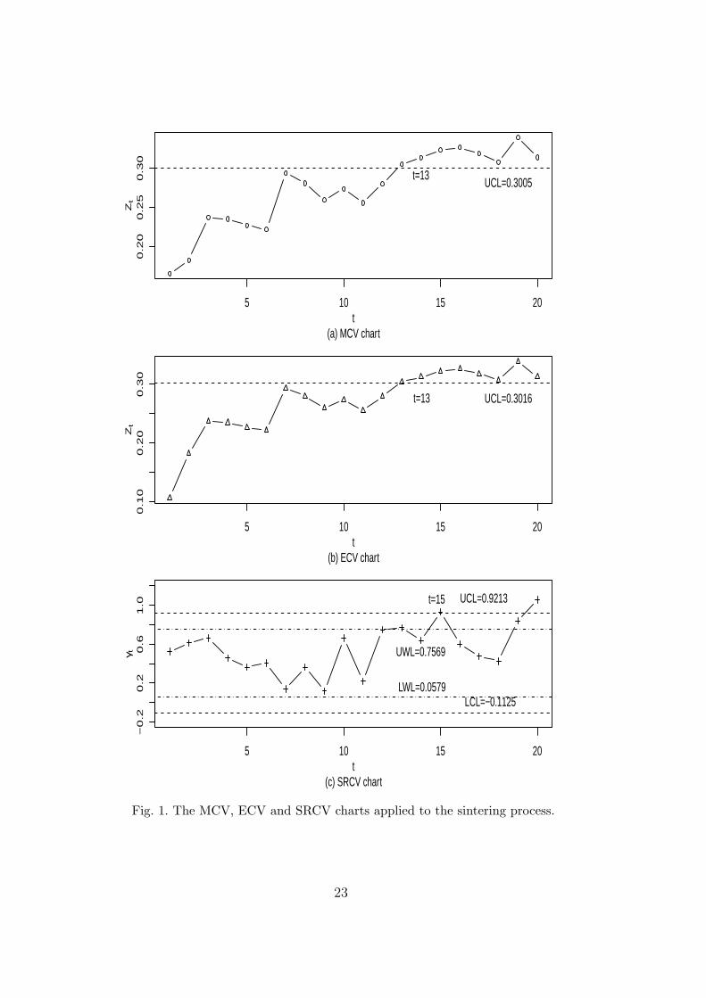
In order to be consistent with Castagliola et al. (2011), 𝜏 ∗ is set to 1.25.The parameters of the new chart which is optimal for detecting a shift from𝛾0 = 0.417 to 𝛾1 = 𝛾0 × 1.25 = 0.521 (i.e. increase of 25%) when 𝑛 = 5are found by the optimizing algorithm to be (𝜆∗, 𝐾∗) = (0.08, 4.3164). UsingEquations (5) and (6), we have 𝜇0(𝛾

2) = 0.1557, 𝜎0(𝛾2) = 0.1643, and the

upper control limit is 0.3005. The Phase I chart (not shown in the paper)seems to confirm that the process is in control.

A second set of data collected during Phase II of the chart implementation arepresented in Table 7 (bottom) of Castagliola et al. (2011). These data consistof 20 new samples taken from the process after the occurrence of a specialcause increasing process variability. The 𝑍𝑡 and the control limit UCL=0.3005are plotted in Figure 1(a). For comparison, we also plot the ECV and SRCVcharts in Figure 1(b) and Figure 1(c). From this Figure, it is observed thatthe our new chart gives an out-of-control signal at observation 13, which isconsistent with the result of Castagliola et al. (2011). With the same dataset,the SRCV chart detects an out-of-control signal at the 15𝑡ℎ sample, which istwo points later than the MCV and ECV charts.

5 Summary and conclusion

The CV control chart extends charting capabilities to non-traditional appli-cations. These include situations where the mean is not constant and/or the

11

variance is a function of the mean, so that it may be possible to insteadplot the CV to achieve statistical control of that parameter. In this paper,a modified EWMA chart is proposed to monitor the CV in order to furtherenhance the sensitivity of the EWMA control chart proposed by Castagliola etal.(2011). It is shown that the newly developed control scheme does not onlydominate most of the existing charts but is also easy to design and implementas illustrated through an application example of real datasets.

Note that our new chart is based on the assumption that each random variablefollows a normal distribution. However, the underlying process is not normalin many applications (Qiu and Li, 2011a,b), and as a result the statisticalproperties of CV charts can be highly affected in such situations. Hence, itis necessary to check how the proposed methodology performs when the un-derlying distribution is violated, which also warrants future research. Futureresearch include a self-starting version of the new CV chart and a study of itsproperties in cases when the IC parameters in the measurement distributionare unknown (Li et al., 2010). Moreover, our chart is constructed under statis-tical design and we believe a control chart for monitoring CV under economicdesign (Zhang, Xie, Goh and Shamsuzzaman, 2011) warrants future research.

Acknowledgement

The authors are grateful to the editor, the associate editor and the anony-mous referees for their valuable comments that have vastly improved thispaper. This research is supported by the Natural Science Foundation of ChinaGrant 11101198, 11201246, 11371202, 11131002, the start-up funding at Liaon-ing University, the RFDP of China Grant 20110031110002 and the PAPD ofJiangsu Higher Education Institutions.

BIBLIOGRAPHY

Breunig, R. (2001). An almost unbiased estimator of the coefficient of varia-tion. Econometric letters. 70(1), 15-19.

Calzada, M.E. and Scariano, S.M. (2013). A synthetic control chart for thecoefficient of variation. Journal of Statistical Computation and Simulation,83(5), 853-867.

Castagliola, P., Achouri, A., Taleb, H., Celano, G. and Psarakis, S. (2013a).Monitoring the coefficient of variation using a variable sampling interval con-trol chart. Quality and Reliability Engineering International, 29(8), 1135-1149.

12

Castagliola, P., Achouri, A., Taleb, H., Celano, G., and Psarakis, S.(2013b).Monitoring the coefficient of variation using control charts with run rules.Quality Technology and Quantitative Management, 10(1), 75-94.

Castagliola, P., Celano, G. and Psarakis, S. (2011). Monitoring the coefficientof variation using EWMA charts. Journal of Quality Technology, 43(3), 249-265.

Celano, G. (2009). Robust design of adaptive control charts for manual manu-facturing/inspection workstations. Journal of Applied statistics. 36, 181-203.

Costa, A.F.B., Machado, M.A.G. (2013). A single chart with supplementaryruns rules for monitoring the mean vector and the covariance matrix of mul-tivariate processes. Computers & Industry Engineering, 66(2), 431-437.

Du, S., Huang, D., and Lv, J. (2013). Recognition of concurrent control chartpatterns using wavelet transform decomposition and multiclass support vectormachines. Computers & Industry Engineering, 66(4), 683-695.

Hendricks, W.A. and Robey, W.K. (1996). The sampling distribution of thecoefficient of variation. Annals of Mathematical Statistics, 7, 129-132.

Hong, E.P., Kang, C.W., Baek, J.W. and Kang, H.W. (2008). Developmentof CV control chart using EWMA technique. Journal of the Society of KoreaIndustrial and Systems Engineering, 31(4), 114-120.

Iglewicz, B., Myers, R.H., and Howe, R.B. (1968). On the percentage pointsof the sample coefficient of variation. Biometrika, 55(3), 580-581.

Kang, C.W., Lee, M.S., Seong, Y.J. and Hawkins, D.M. (2007). A control chartfor the coefficient of variation. Journal of Quality Technology, 39(2), 151-158.

Li, Z., Zhang, J. and Wang, Z. (2010). Self-Starting control chart for simulta-neously monitoring process mean and variance. International Journal of Pro-duction Research, 48 (15), 4537-4553.

Li, Z., Zou, C., Gong, Z. and Wang, Z. (2014). The computation of averagerun length and average time to signal: an overview. Journal of StatisticalComputation and Simulation, 84 (8), 1779-1802.

Mahmoudvand, R. and Hassani, H. (2009). Two new confidence intervals forthe coefficient of variation in a normal distribution. Journal of Applied Statis-tics, 36(4), 429-442.

Mckay, A.T. (1932). Distribution of the coefficient of variation and extendedt distribution. Journal of the Royal Statistical Society, 95, 695-698.

13

Menzefricke, U. (2013a). Control charts for the mean and variance based onchange point methodology. Communications in Statistics-Theory and Meth-ods, 42(6), 988-1007.

Menzefricke, U. (2013b). Combined exponentially weighted moving averagecharts for the mean and variance based on the predictive distribution. Com-munications in Statistics-Theory and Methods, 42(22), 4003-4016.

Qiu, P. and Li, Z. (2011a). On nonparametric statistical process control ofunivariate processes. Technometrics, 53(4), 390-405.

Qiu, P. and Li, Z. (2011b). Distribution-free monitoring of univariate pro-cesses. Statistics and Probability Letters, 81(12), 1833-1840.

Reed, G. F., Lynn, F. and Meade, B. D. (2002). Use of coefficient of vari-ation in assessing variability of quantitative Assays. Clinical and DiagnosticLaboratory Immunology, 9, 1235-1239.

Reh, W. and Scheffler, B. (1996). Significance tests and confidence intervalsfor coefficients of variation. Computational Statistics & Data Analysis, 22(4),449-452

Reynolds, J.M.R. and Stoumbos, Z.G.(2004). Control charts and the efficientallocation of sampling resources. Technometrics 46, 200-214.

Sharpe, W. F. (1994). The Sharpe ratio. Journal of Portfolio Management,21, 49-58.

Tian, L. (2005). Inferences on the common coefficient of variation. Statisticsin Medicine, 24(14), 2213-2220.

Vangel, M.G. (1996). Confidence intervals for a normal coefficient of variation.American Statistician, 15, 21-26.

Verrill, S, Johnson, R.A. (2007). Confidence bounds and hypothesis tests fornormal distribution coefficients of variation. Communications in Statistics-Theory and Methods, 36(12), 2187-2206.

Wu, Z., Yang, M., Jiang, W. and Khoo, M.B.C. (2008). Optimization designsof the combined Shewhart-CUSUM control charts. Computational Statistics& Data Analysis. 53, 496-506.

Zhang, H.Y., Xie, M., Goh, T.N. and Shamsuzzaman, M. (2011). Economicdesign of time-between-events control chart system. Computers & IndustryEngineering, 60, 485-492.

Zhang, J., Zou, C., and Wang, Z. (2010). A control chart based on likelihood

14

ratio test for monitoring process mean and variability. Quality and ReliabilityEngineering International, 26, 63-73.

Zhang, J., Zou, C., and Wang, Z. (2011). A new chart for detecting processmean and variability. Communication in Statistics-Simulation and Computa-tion. 40, 728-743.

15

Table 1𝐾+ values of the upper MCV chart for the selected combinations of 𝜆, 𝛾0 and nwhen IC-ARL=370

n 𝛾0 𝜆 = 0.05 0.1 0.2 0.3 0.5

5 0.05 2.363 2.793 3.254 3.555 3.9620.10 2.439 2.851 3.311 3.613 4.0230.15 2.568 2.964 3.408 3.711 4.1310.20 2.759 3.110 3.555 3.857 4.287

7 0.05 3.322 2.725 3.135 3.398 3.7430.10 2.390 2.773 3.188 3.447 3.7980.15 2.509 2.866 3.269 3.525 3.8790.20 2.666 2.998 3.379 3.633 4.009

10 0.05 2.29 2.666 3.037 3.262 3.5550.10 2.352 2.715 3.077 3.301 3.5990.15 2.451 2.791 3.144 3.371 3.6670.20 2.585 2.901 3.237 3.456 3.766

15 0.05 2.266 2.617 2.949 3.149 3.3980.10 2.309 2.656 2.983 3.184 3.4370.15 2.393 2.715 3.042 3.232 3.4860.20 2.505 2.801 3.110 3.306 3.565

Table 2𝐾− values of the lower MCV chart for the selected combinations of 𝜆, 𝛾0 and nwhen IC-ARL=370

n 𝛾0 𝜆 = 0.05 0.1 0.2 0.3 0.5

5 0.05 1.909 2.024 2.002 1.920 1.7360.10 1.826 1.963 1.956 1.879 1.7030.15 1.699 1.865 1.879 1.814 1.6480.20 1.528 1.732 1.777 1.725 1.575

7 0.05 1.950 2.092 2.102 2.043 1.8920.10 1.875 2.036 2.062 2.006 1.8610.15 1.767 1.951 1.992 1.949 1.8130.20 1.616 1.834 1.904 1.873 1.747

10 0.05 1.982 2.148 2.189 2.148 2.0290.10 1.924 2.105 2.153 2.119 2.0020.15 1.826 2.026 2.095 2.068 1.9600.20 1.697 1.924 2.016 2.002 1.902

15 0.05 2.016 2.197 2.266 2.248 2.1580.10 1.965 2.158 2.236 2.221 2.1360.15 1.885 2.097 2.192 2.180 2.0990.20 1.775 2.012 2.122 2.121 2.049

16

Table 3Optimal couples(𝜆∗,𝐾∗) and zero-state OC-ARLs of the MCV and ECV chartswhen IC-ARL=370

𝜏∗ 𝛾0 = 0.05 𝛾0 = 0.1 𝛾0 = 0.15 𝛾0 = 0.2

n=50.50 (0.35, 1.875) (0.33,1.853) (0.39, 1.741) (0.43, 1.629 )

(4.5, 4.8) (4.5, 4.8) (4.4, 4.8) (4.4, 4.8)0.65 (0.21, 1.995) (0.19, 1.961) (0.18, 1.885) (0.16, 1.781)

(7.9, 8.7) (7.9, 8.8) (7.9, 8.8) (7.8, 8.8)0.80 (0.07, 1.982) (0.05, 1.828) (0.05, 1.699) (0.05, 1.528)

(17.8, 20.6) (17.6, 20.6) (17.2, 20.7) (16.3, 20.9)0.90 (0.05, 1.914) (0.05, 1.831) (0.05, 1.699) (0.05, 1.523)

(43.9, 52.8) (43.4, 54.1) (42.5, 54.3) (41.1, 55.4)1.10 (0.05, 2.363) (0.05, 2.439) (0.05, 2.578) (0.05, 2.759 )

(44.1, 51.2 ) (44.5, 51.5) (46.3, 51.9) (48.5, 52.4)1.25 (0.08, 2.656) (0.08, 2.722) (0.07, 2.759) (0.09, 3.056)

(13.5, 15) (13.7, 15.2) (14.2,15.4) (14.8, 15.9)1.50 (0.15, 3.051) (0.15, 3.115) (0.16, 3.256) (0.14, 3.305)

(5.3, 5.7) (5.4, 5.8) (5.6, 5.9) (5.8, 6.1)2.00 (0.31, 3.579) (0.31, 3.637) (0.23, 3.510) (0.2, 3.545)

(2.3, 2.4) (2.3, 2.4) (2.4, 2.5) (2.5, 2.6)

n=70.50 (0.45, 1.931) (0.55, 1.821) (0.46, 1.841) (0.45, 1.779)

(3.3, 3.4) (3.3, 3.4) (3.3, 3.5) (3.3, 3.5)0.65 (0.29, 2.049) (0.24, 2.043) (0.22, 1.987) (0.21, 1.901)

(5.8, 6.4) (5.9, 6.4) (5.9, 6.4) (5.9, 6.5)0.80 (0.11, 2.102) (0.09, 2.023) (0.09, 2.021) (0.05, 13.0)

(13.5, 15.3) (13.4, 15.4) (13.4, 15.5) (13.0, 15.6)0.90 (0.05, 1.953) (0.05, 1.882) (0.05, 1.767) (0.05, 1.614)

(33.9, 40.3) (33.4, 40.7) (32.7, 41.0) (32.0, 41.6)1.10 (0.05, 2.324) (0.05, 2.392) (0.05, 2.509) (0.05, 2.666)

(34.0, 39.2 ) (34.6, 39.4) (35.8, 40.3) (37.5, 41.0)1.25 (0.11, 2.773) (0.08, 2.656) (0.11, 2.92) (0.12, 3.086)

(10.2, 11.3) (10.5, 11.4) (10.7, 11.7) (11.1, 12)1.50 (0.21, 3.164) (0.13, 2.930) (0.17, 3.164) (0.15, 3.213)

(4.0, 4.3) (4.2, 4.3) (4.2, 4.4) (4.4, 4.6)2.00 (0.25, 3.277) (0.35, 3.555) (0.55, 3.945) (0.35, 3.75)

(1.8, 1.8) (1.8, 1.8) (1.8, 1.9) (1.9, 2.0)

17

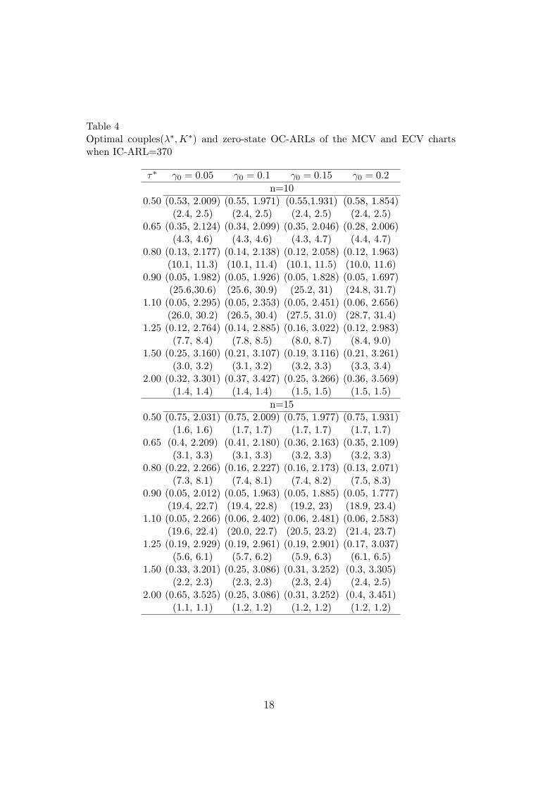
Table 4Optimal couples(𝜆∗,𝐾∗) and zero-state OC-ARLs of the MCV and ECV chartswhen IC-ARL=370

𝜏∗ 𝛾0 = 0.05 𝛾0 = 0.1 𝛾0 = 0.15 𝛾0 = 0.2

n=100.50 (0.53, 2.009) (0.55, 1.971) (0.55,1.931) (0.58, 1.854)

(2.4, 2.5) (2.4, 2.5) (2.4, 2.5) (2.4, 2.5)0.65 (0.35, 2.124) (0.34, 2.099) (0.35, 2.046) (0.28, 2.006)

(4.3, 4.6) (4.3, 4.6) (4.3, 4.7) (4.4, 4.7)0.80 (0.13, 2.177) (0.14, 2.138) (0.12, 2.058) (0.12, 1.963)

(10.1, 11.3) (10.1, 11.4) (10.1, 11.5) (10.0, 11.6)0.90 (0.05, 1.982) (0.05, 1.926) (0.05, 1.828) (0.05, 1.697)

(25.6,30.6) (25.6, 30.9) (25.2, 31) (24.8, 31.7)1.10 (0.05, 2.295) (0.05, 2.353) (0.05, 2.451) (0.06, 2.656)

(26.0, 30.2) (26.5, 30.4) (27.5, 31.0) (28.7, 31.4)1.25 (0.12, 2.764) (0.14, 2.885) (0.16, 3.022) (0.12, 2.983)

(7.7, 8.4) (7.8, 8.5) (8.0, 8.7) (8.4, 9.0)1.50 (0.25, 3.160) (0.21, 3.107) (0.19, 3.116) (0.21, 3.261)

(3.0, 3.2) (3.1, 3.2) (3.2, 3.3) (3.3, 3.4)2.00 (0.32, 3.301) (0.37, 3.427) (0.25, 3.266) (0.36, 3.569)

(1.4, 1.4) (1.4, 1.4) (1.5, 1.5) (1.5, 1.5)

n=150.50 (0.75, 2.031) (0.75, 2.009) (0.75, 1.977) (0.75, 1.931)

(1.6, 1.6) (1.7, 1.7) (1.7, 1.7) (1.7, 1.7)0.65 (0.4, 2.209) (0.41, 2.180) (0.36, 2.163) (0.35, 2.109)

(3.1, 3.3) (3.1, 3.3) (3.2, 3.3) (3.2, 3.3)0.80 (0.22, 2.266) (0.16, 2.227) (0.16, 2.173) (0.13, 2.071)

(7.3, 8.1) (7.4, 8.1) (7.4, 8.2) (7.5, 8.3)0.90 (0.05, 2.012) (0.05, 1.963) (0.05, 1.885) (0.05, 1.777)

(19.4, 22.7) (19.4, 22.8) (19.2, 23) (18.9, 23.4)1.10 (0.05, 2.266) (0.06, 2.402) (0.06, 2.481) (0.06, 2.583)

(19.6, 22.4) (20.0, 22.7) (20.5, 23.2) (21.4, 23.7)1.25 (0.19, 2.929) (0.19, 2.961) (0.19, 2.901) (0.17, 3.037)

(5.6, 6.1) (5.7, 6.2) (5.9, 6.3) (6.1, 6.5)1.50 (0.33, 3.201) (0.25, 3.086) (0.31, 3.252) (0.3, 3.305)

(2.2, 2.3) (2.3, 2.3) (2.3, 2.4) (2.4, 2.5)2.00 (0.65, 3.525) (0.25, 3.086) (0.31, 3.252) (0.4, 3.451)

(1.1, 1.1) (1.2, 1.2) (1.2, 1.2) (1.2, 1.2)

18

Table 5OC-ARLs of the MCV and ECV charts when IC-ARL=370

n=5 n=7 n=10 n=15𝜆 𝛾0 𝜏 MCV ECV MCV ECV MCV ECV MCV ECV

0.05 0.1 1.00 370 370 370 370 370 370 370 3701.05 98.6 113.6 80.2 93.2 63.6 74.3 48.5 56.81.10 44.8 51.2 34.5 39.8 26.7 30.3 20.0 22.71.15 26.7 30.2 20.4 23.3 15.9 17.8 12.0 13.51.20 18.5 20.8 14.3 16.0 11.1 12.4 8.5 9.61.25 13.9 15.6 10.8 12.1 8.5 9.5 6.6 7.31.50 6.1 6.7 4.8 5.3 3.9 4.3 3.1 3.42.00 2.8 3.1 2.3 2.5 1.9 2.1 1.6 1.7

0.2 1.00 370 370 370 370 370 370 370 3701.05 103.9 113.6 84.6 93.6 67.8 75.6 51.7 58.31.10 48.1 52.3 37.2 40.9 28.8 31.7 21.7 23.71.15 29.1 31.2 22.4 24.2 17.3 18.7 13.1 14.31.20 20.3 21.7 15.6 16.9 12.1 13.1 9.3 10.11.25 15.3 16.3 11.9 12.8 9.3 10.0 7.2 7.81.50 6.7 7.1 5.3 5.7 4.2 4.5 3.3 3.62.00 3.1 3.3 2.5 2.7 2.1 2.2 1.7 1.8

0.1 0.1 1.00 370 370 370 370 370 370 370 3701.05 112.6 127.0 91.6 105.7 72.8 84.6 55.9 64.31.10 50.1 57.4 37.9 43.7 28.4 32.7 20.8 23.41.15 28.4 32.5 21.2 24.1 15.9 17.8 11.7 12.91.20 18.9 21.2 14.1 15.7 10.7 11.8 7.9 8.71.25 13.4 15.2 10.4 11.4 7.9 8.7 6.0 6.51.50 5.6 6.0 4.4 4.7 3.4 3.7 2.7 2.92.00 2.6 2.7 2.1 2.2 1.7 1.8 1.4 1.5

0.2 1.00 370 370 370 370 370 370 370 3701.05 117.3 129.4 96.6 106.5 77.3 86.6 58.0 66.21.10 52.9 58.6 40.4 44.8 30.4 34.1 21.9 24.31.15 30.2 33.5 22.7 24.8 17.0 18.6 12.4 13.51.20 20.2 21.8 15.2 16.4 11.5 12.4 8.5 9.11.25 14.8 16.0 11.2 12.0 8.6 9.2 6.4 6.91.50 6.0 6.4 4.7 4.9 3.7 3.9 2.9 3.12.00 2.8 2.9 2.1 2.3 1.8 1.9 1.5 1.5

19

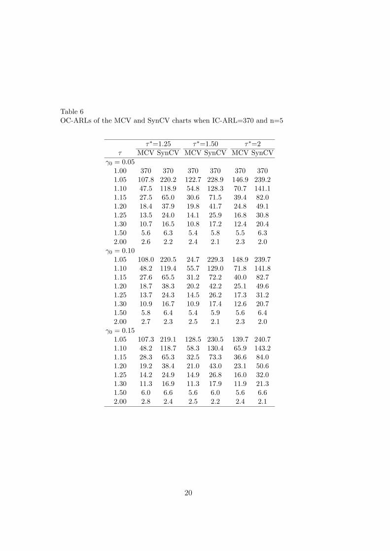
Table 6OC-ARLs of the MCV and SynCV charts when IC-ARL=370 and n=5

𝜏∗=1.25 𝜏∗=1.50 𝜏∗=2𝜏 MCV SynCV MCV SynCV MCV SynCV

𝛾0 = 0.051.00 370 370 370 370 370 3701.05 107.8 220.2 122.7 228.9 146.9 239.21.10 47.5 118.9 54.8 128.3 70.7 141.11.15 27.5 65.0 30.6 71.5 39.4 82.01.20 18.4 37.9 19.8 41.7 24.8 49.11.25 13.5 24.0 14.1 25.9 16.8 30.81.30 10.7 16.5 10.8 17.2 12.4 20.41.50 5.6 6.3 5.4 5.8 5.5 6.32.00 2.6 2.2 2.4 2.1 2.3 2.0

𝛾0 = 0.101.05 108.0 220.5 24.7 229.3 148.9 239.71.10 48.2 119.4 55.7 129.0 71.8 141.81.15 27.6 65.5 31.2 72.2 40.0 82.71.20 18.7 38.3 20.2 42.2 25.1 49.61.25 13.7 24.3 14.5 26.2 17.3 31.21.30 10.9 16.7 10.9 17.4 12.6 20.71.50 5.8 6.4 5.4 5.9 5.6 6.42.00 2.7 2.3 2.5 2.1 2.3 2.0

𝛾0 = 0.151.05 107.3 219.1 128.5 230.5 139.7 240.71.10 48.2 118.7 58.3 130.4 65.9 143.21.15 28.3 65.3 32.5 73.3 36.6 84.01.20 19.2 38.4 21.0 43.0 23.1 50.61.25 14.2 24.9 14.9 26.8 16.0 32.01.30 11.3 16.9 11.3 17.9 11.9 21.31.50 6.0 6.6 5.6 6.0 5.6 6.62.00 2.8 2.4 2.5 2.2 2.4 2.1

20

Table 7OC-ARLs of the MCV and SynCV charts when IC-ARL=370 and n=10

𝜏∗=1.25 𝜏∗=1.50 𝜏∗=2𝜏 MCV SynCV MCV SynCV MCV SynCV

𝛾0 = 0.051.00 370 370 370 370 370 3701.05 76.3 195.6 96.2 208.2 104.9 218.81.10 29.2 84.4 36.8 95.9 41.5 106.71.15 15.9 38.0 18.7 44.5 20.7 51.61.20 10.5 19.5 11.6 22.6 12.4 26.81.25 7.8 11.5 8.0 12.8 8.5 15.31.30 6.1 7.6 6.1 8.1 6.3 9.51.50 3.3 3.0 3.0 2.7 3.0 2.92.00 1.6 1.3 1.5 1.3 1.4 1.2

𝛾0 = 0.101.05 80.3 196.2 91.5 209.4 112.3 219.71.10 30.5 85.3 35.0 97.1 44.9 107.81.15 16.5 38.6 18.1 45.3 22.7 52.41.20 10.7 19.8 11.3 23.1 13.5 27.31.25 7.9 11.7 8.0 13.1 9.1 15.61.30 6.1 7.8 6.1 8.3 6.6 9.81.50 3.3 3.0 3.1 2.8 3.1 3.02.00 1.6 1.3 1.5 1.3 1.4 1.2

𝛾0 = 0.151.05 85.0 197.3 90.3 210.6 99.2 221.21.10 32.6 86.5 34.6 98.7 38.3 109.71.15 17.2 39.4 18.0 46.4 19.6 53.81.20 11.1 20.4 11.4 23.8 12.1 28.21.25 8.1 12.1 8.1 13.6 8.4 16.21.30 6.3 8.1 6.3 8.6 6.4 10.11.50 3.3 3.1 3.2 2.9 3.2 3.12.00 1.6 1.4 1.6 1.3 1.5 1.3

21

Table 8OC-ARLs of the MCV and SRCV charts when IC-ARL=370 and 𝜆 = 0.05

𝛾0 = 0.05 𝛾0 = 0.1 𝛾0 = 0.15 𝛾0 = 0.2n 𝜏 MCV SRCV MCV SRCV MCV SRCV MCV SRCV

5 0.5 8.4 6.2 8.2 6.2 7.9 6.3 7.5 6.30.6 10.2 11.8 10.0 11.8 9.7 12.0 9.1 12.20.7 13.7 28.4 13.4 28.6 13.0 29.0 12.3 29.50.8 22.3 80.0 21.9 80.6 21.4 81.6 20.5 83.00.9 60.8 236.5 60.3 237.5 59.8 239.3 58.8 241.61.1 61.5 144.5 62.7 145.3 64.4 146.6 67.2 148.41.2 22.7 54.4 23.2 54.9 23.9 55.8 25.3 57.01.5 7.0 11.8 7.1 12.0 7.4 12.2 7.8 12.62.0 3.1 5.6 3.2 5.7 3.3 5.7 3.5 5.9

10 0.5 5.6 4.1 5.5 4.1 5.4 4.1 5.2 4.10.6 6.7 5.0 6.6 5.0 6.5 5.0 6.2 5.10.7 8.7 8.9 8.6 9.0 8.4 9.1 8.1 9.30.8 13.4 26.1 13.3 26.4 13.1 26.9 12.7 27.60.9 33.2 119.1 33.1 120.3 32.9 122.1 32.5 124.61.1 34.0 86.9 34.7 87.7 35.6 89.2 37.3 91.21.2 13.1 25.6 13.4 26.0 13.9 26.6 14.6 27.51.5 4.4 6.2 4.4 6.3 4.6 6.4 4.8 6.62.0 2.1 4.2 2.1 4.3 2.2 4.3 2.3 4.3

15 0.5 4.6 4.0 4.5 4.0 4.4 4.0 4.3 4.00.6 5.4 4.2 5.3 4.2 5.2 4.2 5.1 4.20.7 6.9 5.8 6.8 5.8 6.7 5.9 6.6 6.00.8 10.4 14.4 10.3 14.6 10.2 14.9 10.0 15.30.9 24.5 75.3 24.4 76.2 24.2 77.6 24.0 79.61.1 24.7 60.9 25.3 61.6 26.1 62.9 27.2 64.71.2 9.9 16.6 10.1 16.8 10.5 17.3 11.0 17.91.5 3.4 4.9 3.5 5.0 3.6 5.0 3.8 5.12.0 1.7 4.1 1.7 4.1 1.8 4.1 1.9 4.1

22

5 10 15 20

0.2

00

.25

0.3

0

t

Zt

UCL=0.3005t=13

(a) MCV chart

5 10 15 20

0.1

00

.20

0.3

0

t

Zt

UCL=0.3016t=13

(b) ECV chart

5 10 15 20

−0

.20

.20

.61

.0

t

γ t

UCL=0.9213

LCL=−0.1125

UWL=0.7569

LWL=0.0579

t=15

(c) SRCV chart

Fig. 1. The MCV, ECV and SRCV charts applied to the sintering process.

23