design of experiments for the nips 2003 variable selection benchmark isabelle guyon...

Design of experiments for the NIPS 2003 variable selection benchmark Isabelle Guyon – July 2003

[email protected]

Background: Results published in the field of feature or variable selection (see e.g. the special issue of JMLR on variable and feature selection: http://www.jmlr.org/papers/special/feature.html) are for the most part on different data sets or used different data splits, which make them hard to compare. We formatted a number of datasets for the purpose of benchmarking variable selection algorithms in a controlled manner1. The data sets were chosen to span a variety of domains (cancer prediction from mass-spectrometry data, handwritten digit recognition, text classification, and prediction of molecular activity). One dataset is artificial. We chose data sets that had sufficiently many examples to create a large enough test set to obtain statistically significant results. The input variables are continuous or binary, sparse or dense. All problems are two-class classification problems. The similarity of the tasks allows participants to enter results on all data sets. Other problems will be added in the future. Method: Preparing the data included the following steps:

- Preprocessing data to obtain features in the same numerical range (0 to 999 for continuous data and 0/1 for binary data).

- Adding “random” features distributed similarly to the real features. In what follows we refer to such features as probes to distinguish them from the real features. This will allow us to rank algorithms according to their ability to filter out irrelevant features.

- Randomizing the order of the patterns and the features to homogenize the data. - Training and testing on various data splits using simple feature selection and

classification methods to obtain baseline performances. - Determining the approximate number of test examples needed for the test set to

obtain statistically significant benchmark results using the rule-of-thumb ntest = 100/p, where p is the test set error rate (see What size test set gives good error rate estimates? I. Guyon, J. Makhoul, R. Schwartz, and V. Vapnik. PAMI, 20 (1), pages 52--64, IEEE. 1998, http://www.clopinet.com/isabelle/Papers/test-size.ps.Z). Since the test error rate of the classifiers of the benchmark is unknown, we used the results of the baseline method and added a few more examples.

- Splitting the data into training, validation and test set. The size of the validation set is usually smaller than that of the test set to keep as much training data as possible.

Both validation and test set truth-values (labels) are withheld during the benchmark. The validation set serves as development test set. During the time allotted to the participants to try methods on the data, participants are allowed to send the validation set results (in 1 In this document, we do not make a distinction between features and variables. The benchmark addresses the problem of selecting input variables. Those may actually be features derived from the original variables using a preprocessing.

the form of classifier outputs) and obtain result scores. Such score are made available to all participants to stimulate research. At the end of the benchmark, the participants send their test set results. The scores on the test set results are disclosed simultaneously to all participants after the benchmark is over. Data formats: All the data sets are in the same format and include 8 files in ASCII format: dataname.param: Parameters and statistics about the data dataname.feat: Identities of the features (in the order the features are found in the data). dataname_train.data: Training set (a spase or a regular matrix, patterns in lines, features in columns). dataname_valid.data: Validation set. dataname_test.data: Test set. dataname_train.labels: Labels (truth values of the classes) for training examples. dataname_valid.labels: Validation set labels (withheld during the benchmark). dataname_test.labels: Test set labels (withheld during the benchmark). The matrix data formats used are:

- For regular matrices: a space delimited file with a new-line character at the end of each line.

- For sparse matrices with binary values: for each line of the matrix, a space delimited list of indices of the non-zero values. A new-line character at the end of each line.

- For sparse matrices with non-binary values: for each line of the matrix, a space delimited list of indices of the non-zero values followed by the value itself, separated from it index by a colon. A new-line character at the end of each line.

The results on each dataset should be formatted in 7 ASCII files: dataname_train.resu: +-1 classifier outputs for training examples (mandatory for final submissions). dataname_valid.resu: +-1 classifier outputs for validation examples (mandatory for development and final submissions). dataname_test.resu: +-1 classifier outputs for test examples (mandatory for final submissions). dataname_train.conf: confidence values for training examples (optional). dataname_valid.conf: confidence values for validation examples (optional). dataname_test.conf: confidence values for test examples (optional). dataname.feat: list of features selected (one integer feature number per line, starting from one, ordered from the most important to the least important if such order exists). If no list of features is provided, it will be assumed that all the features were used. Format for classifier outputs: - All .resu files should have one +-1 integer value per line indicating the prediction for the various patterns. - All .conf files should have one decimal positive numeric value per line indicating classification confidence. The confidence values can be the absolute discriminant values. They do not need to be normalized to look like probabilities. They will be used to compute ROC curves and Area Under such Curve (AUC).

Result rating: The classification results are rated with the balanced error rate (the average of the error rate on training examples and on test examples). The area under the ROC curve is also be computed, if the participants provide classification confidence scores in addition to class label predictions. But the relative strength of classifiers is judged only on the balanced error rate. The participants are invited to provide the list of features used. For methods having performance differences that are not statistically significant, the method using the smallest number of features wins . If no feature set is provided, it is assumed that all the features were used. The organizers may then provide the participants with one or several test sets containing only the features selected to verify the accuracy of the classifier when it uses those features only. The proportion of random probes in the feature set is also be computed. It is used to assess the relative strength of method with non-statistically significantly different error rates and a relative difference in number of features that is less than 5%. In that case, the method with smallest number of random probes in the feature set wins . Dataset A: ARCENE

1) Topic The task of ARCENE is to distinguish cancer versus normal patterns from mass-spectrometric data. This is a two-class classification problem with continuous input variables.

2) Sources a. Original owners

The data were obtained from two sources: The National Cancer Institute (NCI) and the Eastern Virginia Medical School (EVMS). All the data consist of mass-spectra obtained with the SELDI technique. The samples include patients with cancer (ovarian or prostate cancer), and healthy or control patients. NCI ovarian data: The data were originally obtained from http://clinicalproteomics.steem.com/download-ovar.php. We use the 8/7/02 data set: http://clinicalproteomics.steem.com/Ovarian%20Dataset%208-7-02.zip. The data includes 253 spectra, including 91 controls and 162 cancer spectra. Number of features: 15154. NCI prostate cancer data: The data were originally obtained from http://clinicalproteomics.steem.com/JNCI%20Data%207-3-02.zip on the web page http://clinicalproteomics.steem.com/download-prost.php. There are a total of 322 samples: 63 samples with no evidence of disease and PSA level less than 1; 190 samples with benign prostate with PSA levels greater than 4; 26 samples with prostate cancer with PSA levels 4 through 10; 43 samples with prostate cancer with PSA levels greater than 10. Therefore, there are 253 normal samples and 69 disease samples. The original training set is composed of 56 samples:

• 25 samples with no evidence of disease and PSA level less than 1 ng/ml. • 31 biopsy-proven prostate cancer with PSA level larger than 4 ng/ml.

But the exact split is not given in the paper or on the web site. The original test set contains the remaining 266 samples (38 cancer and 228 normal). Number of features: 15154. EVMS prostate cancer data: The data is downloadable from: http://www.evms.edu/vpc/seldi/. The training data data includes 652 spectra from 326 patients (spectra are in duplicate) and includes 318 controls and 334 cancer spectra. Study population: 167 prostate cancer (84 state 1 and 2; 83 stage 3 and 4), 77 benign prostate hyperplasia, and 82 age-matched normals. The test data includes 60 additional patients. The labels for the test set are not provided with the data, so the test spectra are not used for the benchmark. Number of features: 48538.

b. Donor of database This version of the database was prepared for the NIPS 2003 variable and feature selection benchmark by Isabelle Guyon, 955 Creston Road, Berkeley, CA 94708, USA ([email protected]).

c. Date received: August 2003.

3) Past usage NCI ovarian cancer original paper: “Use of proteomic patterns in serum to identify ovarian cancer Emanuel F Petricoin III, Ali M Ardekani, Ben A Hitt, Peter J Levine, Vincent A Fusaro, Seth M Steinberg, Gordon B Mills, Charles Simone, David A Fishman, Elise C Kohn, Lance A Liotta. THE LANCET • Vol 359 • February 16, 2002 • www.thelancet.com” are so far not reproducible. Note: The data used is a newer set of spectra obtained after the publication of the paper and of better quality. 100% accuracy is easily achieved on the test set using various data splits on this version of the data. NCI prostate cancer original paper: Serum proteomic patterns for detection of prostate cancer. Petricoin et al. Journal of the NCI, Vol. 94, No. 20, Oct. 16, 2002. The test results of the paper are shown in Table A.1. FP FN TP TN Error 1-error Specificity Sensitivity 51 2 36 177 20.30% 79.70% 77.63% 94.74%

Table A.1: Results of Petricoin et al. on the NCI prostate cancer data. Fp=false positive, FN=false negative, TP=true positive, TN=true negative.

Error=(FP+FN)/(FP+FN+TP+TN), Specificity=TN/(TN+FP), Sensitivity=TP/(TP+FN). EVMS prostate cancer original paper: Serum Protein Fingerprinting Coupled with a Pattern-matching Algorithm Distinguishes Prostate Cancer from Benign Prostate Hyperplasia and Healthy Men, Bao-Ling Adam, et al., CANCER RESEARCH 62, 3609–3614, July 1, 2002.

In the following excerpt from the original paper some baseline results are reported: “Surface enhanced laser desorption/ionization mass spectrometry protein profiles of serum from 167 PCA patients, 77 patients with benign prostate hyperplasia, and 82 age-matched unaffected healthy men were used to train and develop a decision tree classification algorithm that used a nine-protein mass pattern that correctly classified 96% of the samples. A blinded test set, separated from the training set by a stratified random sampling before the analysis, was used to determine the sensitivity and specificity of the classification system. A sensitivity of 83%, a specificity of 97%, and a positive predictive value of 96% for the study population and 91% for the general population were obtained when comparing the PCA versus noncancer (benign prostate hyperplasia/healthy men) groups.”

4) Experimental design We merge the datasets from the three different sources (253+322+326=901 samples). We obtained 91+253+159=503 control samples (negative class) and 162+69+167=398 cancer samples (positive class). The motivations for merging datasets include:

- Obtaining enough data to be able to cut a sufficient size test set. - Creating a problem where possibly non-linear classifiers and non-linear feature

selection methods might outperform linear methods. The reason is that there will be in each class different clusters corresponding differences in disease, gender, and sample preparation.

- Finding out whether there are features that are generic of the separation cancer vs. normal across various cancers.

We designed a preprocessing that is suitable for mass-spec data and applied it to all the data sets to reduce the disparity between data sources. The preprocessing consists of the following steps:

- Limiting the mass range: We eliminated small masses under m/z=200 that include usually chemical noise specific to the MALDI/SELDI process (influence of the “matrix”). We also eliminated large masses over m/z=10000 because few features are usually relevant in that domain and we needed to compress the data.

- Averaging the technical repeats: In the EVMS data, two technical repeats were available. We averaged them because we wanted to have examples in the test set that are independent so that we can apply simple statistical tests.

- Removing the baseline: We subtracted in a window the median of the 20% smallest values. An example of baseline detection is shown in Figure A.1.

- Smoothing: The spectra were slightly smoothed with an exponential kernel in a window of size 9.

- Re-scaling: The spectra were divided by the median of the 5% top values. - Taking the square root. The square root of the all values was taken. - Aligning the spectra: We slightly shifted the spectra collections of the three

datasets so that the peaks of the average spectrum would be better aligned (Figures A.2 and A.3). As a result, the mass-over-charge (m/z) values that identify the features in the aligned data are imprecise. We took the NCI prostate cancer m/z as reference.

- Limiting more the mass range: To eliminate border effects, the spectra border were cut.

- Soft thresholding the values: After examining the distribution of values in the data matrix, we subtracted a threshold and equaled to zero all the resulting values that were negative. In this way, we kept only about 50% of non-zero value, which represents significant data compression (see Figure A.4).

- Quantizing: We quantized the values to 1000 levels. The resulting data set including all training and test data merged from the three sources has 901 patterns from 2 classes and 9500 features. We remove one pattern to obtain the round number 900. At every step, we checked that the change in performance of a linear SVM classifier trained and tested on a random split of the data was not significant. On that basis, we have some confidence that our preprocessing did not alter significantly the information content of the data. We further manipulated the data to add random “probes”:

- We identified the region of the spectra with least information content using an interval search for the region that gave worst prediction performance of a linear SVM (indices 2250-4750). We replaced the features in that region by “random probes” obtained by randomly permuting the values in the columns of the data matrix.

- We identified another region of low information content: 6500-7000. We added 500 random probes that are permutations of those features.

After such manipulations, the data had 10000 features, including 7000 real features and 3000 random probes. The reason for not adding more probes is purely practical: non-sparse data cannot be compressed sufficiently to be stored and transferred easily in the context of a benchmark.

0 2000 4000 6000 8000 10000 12000 14000 160000

10

20

30

40

50

60

70

80

90

100

Figure A.1: Example of baseline detection (EVMS data).

3000 4000 5000 6000 7000 8000 9000 10000 11000-0.5

0

0.5

1

1.5

2

Figure A.2: Central part of the spectra before alignment. We show in red the average NCI ovarian spectra, in blue the average NCI prostate spectra, and in green the average EVMS prostate spectra.

3000 4000 5000 6000 7000 8000 9000 10000 11000-0.5

0

0.5

1

1.5

2

Figure A.3: Central part of the spectra after alignment. We show in red the average NCI ovarian spectra, in blue the average NCI prostate spectra, and in green the average EVMS prostate spectra.

0 100 200 300 400 500 600 700 800 900 10000

0.5

1

1.5

2

2.5

3

3.5

4

4.5

5x 10

6

Figure A.4: Distributions of the values in the ARCENE data after preprocessing.

1000 2000 3000 4000 5000 6000 7000 8000 9000 10000

10

20

30

40

50

60

70

80

90

100 0

50

100

150

200

250

300

350

400

450

500

Figure A.5: Heat map of the training set of the ARCENE data. We represent the data matrix (patients in line and features in columns). The values are clipped at 500 to increase the contrast. The values are then mapped to colors according to the color-map on the right. The stripe beyond the 10000 feature index indicated the class labels: +1=red, -1=green.

5) Number of examples and class distribution

Positive ex. Negative ex. Total Check sum Training set 44 56 100 70726744 Validation set 44 56 100 71410108 Test set 310 390 700 493023349 All 398 502 900 635160201

6) Type of input variables and variable statistics

Real variables Random probes Total 7000 3000 10000 All variables are integer quantized on 1000 levels. There are no missing values. The data is not very sparse, but for data compression reasons, we thresholded the values. Approximately 50% of the entries are non zero. The data was saved as a non-sparse matrix.

7) Results of the run of the lambda method and linear SVM Before the benchmark, we ran some simple methods to determine what an appropriate number of examples should be. The “lambda” method (provided with the sample code) had approximately a 30% test error rate ans a linear SVM trained on all features a 15% error rate. The rule of thumb number_of_test_examples=100/test_errate=100/.15=667 led us to keep 700 examples for testing. The best benchmark error rates are of the order 15%, which confirms that our estimate was correct. Dataset B: GISETTE

1) Topic The task of GISETTE is to discriminate between to confusable handwritten digits: the four and the nine. This is a two-class classification problem with sparse continuous input variables.


The data set was constructed from the MNIST data that is made available by Yann LeCun of the NEC Research Institute at http://yann.lecun.com/exdb/mnist/. The digits have been size-normalized and centered in a fixed-size image of dimension 28x28. We show examples of digits in Figure B1.

Figure B1: Two examples of digits from the MNIST database. We used only examples of fours and nines to prepare our dataset.



3) Past usage Many methods have been tried on the MNIST database. Here is an abbreviated list from http://yann.lecun.com/exdb/mnist/:

METHOD TEST ERROR RATE (%) linear classifier (1-layer NN) 12.0

linear classifier (1-layer NN) [deskewing] 8.4

pairwise linear classifier 7.6 K-nearest-neighbors, Euclidean 5.0

K-nearest-neighbors, Euclidean, deskewed 2.4

40 PCA + quadratic classifier 3.3 1000 RBF + linear classifier 3.6

K-NN, Tangent Distance, 16x16 1.1

SVM deg 4 polynomial 1.1 Reduced Set SVM deg 5 polynomial 1.0

Virtual SVM deg 9 poly [distortions] 0.8

2-layer NN, 300 hidden units 4.7 2-layer NN, 300 HU, [distortions] 3.6

2-layer NN, 300 HU, [deskewing] 1.6

2-layer NN, 1000 hidden units 4.5

5 10 15 20 25

5

10

15

20

25

5 10 15 20 25

5

10

15

20

25

2-layer NN, 1000 HU, [distortions] 3.8 3-layer NN, 300+100 hidden units 3.05

3-layer NN, 300+100 HU [distortions] 2.5

3-layer NN, 500+150 hidden units 2.95 3-layer NN, 500+150 HU [distortions] 2.45

LeNet-1 [with 16x16 input] 1.7

LeNet-4 1.1 LeNet-4 with K-NN instead of last layer 1.1

LeNet-4 with local learning instead of ll 1.1

LeNet-5, [no distortions] 0.95 LeNet-5, [huge distortions] 0.85

LeNet-5, [distortions] 0.8

Boosted LeNet-4, [distortions] 0.7 K-NN, shape context matching 0.67

Reference: Y. LeCun, L. Bottou, Y. Bengio, and P. Haffner. "Gradient-based learning applied to document recognition." Proceedings of the IEEE, 86(11):2278-2324, November 1998. http://yann.lecun.com/exdb/publis/index.html#lecun-98

4) Experimental design To construct the dataset, we performed the following steps:

- We selected a random subset of the “four” and “nine” patterns from the training and test sets of the MNIST.

- We normalized the database so that the pixel values would be in the range [0, 1]. We thresholded values below 0.5 to increase data sparsity.

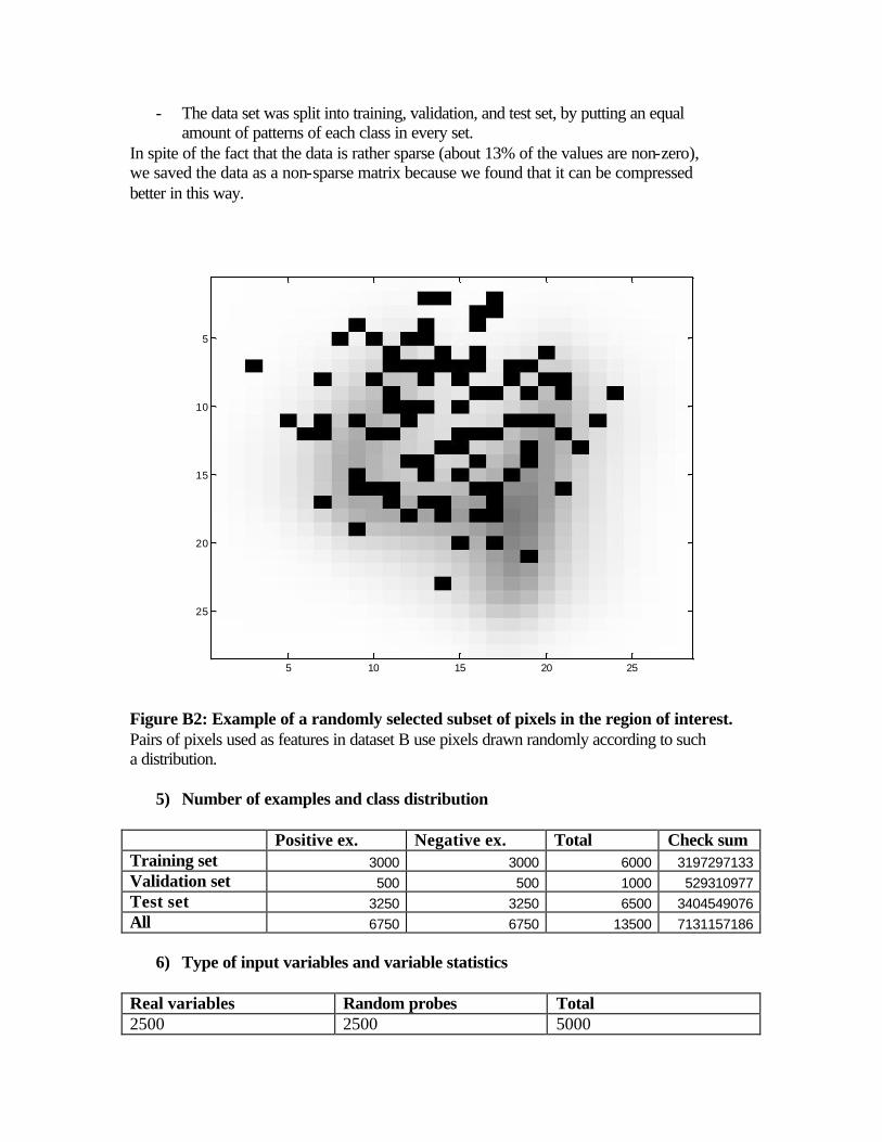
- We constructed a feature set, which consists of the original variables (normalized pixels) plus a randomly selected subset of products of pairs of variables. The pairs were sampled such that each pair member is normally distributed in a region of the image slightly biased upwards. The rationale beyond this choice is that pixels that are discriminative of the “four/nine” separation are more likely to fall in that region (See Figure B2).

- We eliminated all features that had only zero values. - Of the remaining features, we selected all the original pixels and complemented

them with pairs to attain the number of 2500 features. - Another 2500 pairs were used to construct “probes”: the values of the features

were individually permuted across patterns (column randomization). In this way we obtained probes that are similarly distributed to the other features.

- We randomized the order of the features. - We quantized the data to 1000 levels.

- The data set was split into training, validation, and test set, by putting an equal amount of patterns of each class in every set.

In spite of the fact that the data is rather sparse (about 13% of the values are non-zero), we saved the data as a non-sparse matrix because we found that it can be compressed better in this way.

5 10 15 20 25

5

10

15

20

25

Figure B2: Example of a randomly selected subset of pixels in the region of interest. Pairs of pixels used as features in dataset B use pixels drawn randomly according to such a distribution.




Real variables Random probes Total 2500 2500 5000

All variables are integer quantized on 1000 levels. There are no missing values. The data is rather sparse. Approximately 13% of the entries are non zero. The data was saved as a non-sparse matrix, because it compresses better in that format.

7) Results of the runs of the lambda and baseline methods Before the benchmark, we ran some simple methods to determine what an appropriate number of examples should be. The “lambda” method (provided with the sample code) had approximately a 30% test error rate and a linear SVM trained on all features a 3.5% error rate. The rule of thumb number_of_test_examples=100/test_errate=100/ 0.035= 2857. However, other explorations we made with on-linear SVMs and the examination of previous performances obtained on the entire MNIST dataset indicate that the best error rates could be below 2%. A test set of 6500 example should allow error rates as low as 1.5%. This motivated our test set size choice. The best benchmark error rates confirmed that our estimate was just right. Dataset C: DEXTER

1) Topic The task of DEXTER is to filter texts about "corporate acquisitions". This is a two-class classification problem with sparse continuous input variables.


The original data set we used is a subset of the well-known Reuters text categorization benchmark. The data was originally collected and labeled by Carnegie Group, Inc. and Reuters, Ltd. in the course of developing the CONSTRUE text categorization system. It is hosted by the UCI KDD repository: http://kdd.ics.uci.edu/databases/reuters21578/reuters21578.html. David D. Lewis is hosting valuable resources about this data (see http://www.daviddlewis.com/resources/testcollections/reuters21578/). We used the “corporate acquisition” text classification class pre-processed by Thorsten Joachims <[email protected]>. The data is one of the examples of the software package SVM-Light., see http://svmlight.joachims.org/. The example can be downloaded from ftp://ftp-ai.cs.uni-dortmund.de/pub/Users/thorsten/svm_light/examples/example1.tar.gz.



3) Past usage Hundreds of articles have appeared on this data. For a list see: http://kdd.ics.uci.edu/databases/reuters21578/README.txt

Also, 446 citations including “Reuters” were found on CiteSeer: http://citeseer.nj.nec.com.

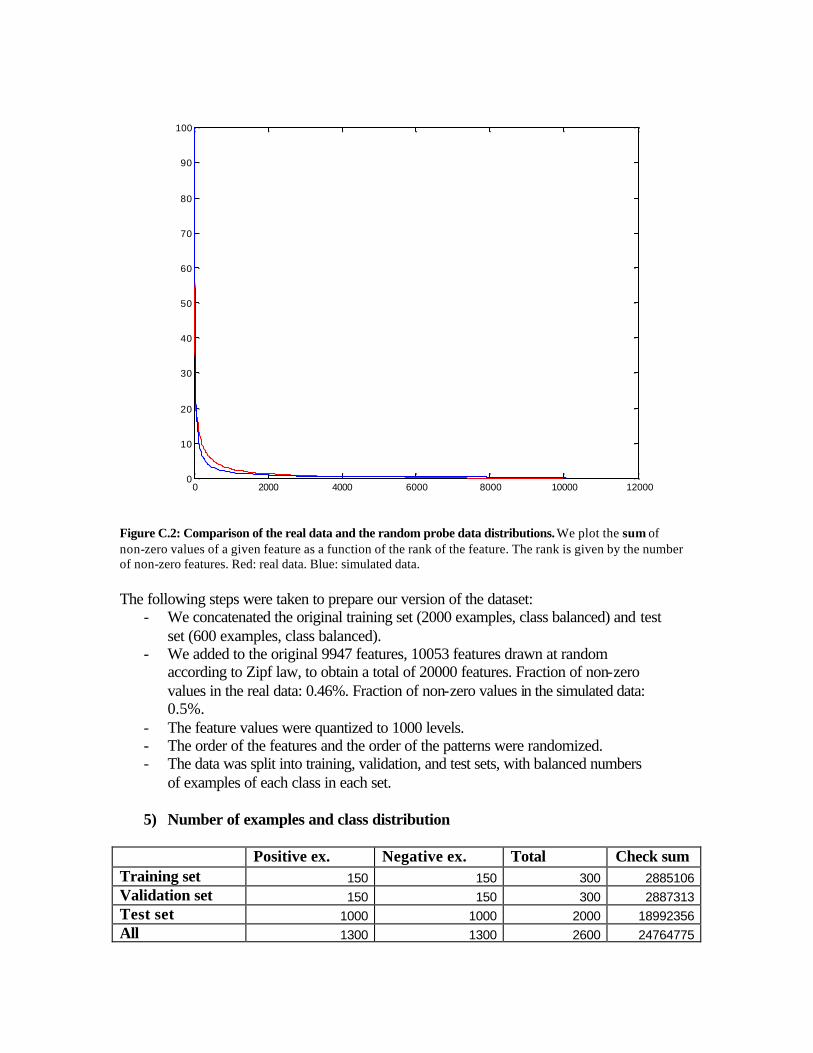
4) Experimental design The original data formatted by Thorsten Joachims is in the “bag-of-words” representation. There are 9947 features (of which 2562 are always zeros for all the examples) that represent frequencies of occurrence of word stems in text. Some normalizations have been applied that are not detailed by Thorsten Joachims in his documentation. The task is to learn which Reuters articles are about "corporate acquisitions". The frequency of appearance of words in text is known to follow approximately Zipf’s law (for details, see e.g. http://linkage.rockefeller.edu/wli/zipf/). According to that law, the frequency of occurrence of words, as a function of the rank k when the rank is determined by the frequency of occurrence, is a power-law function Pk ~ 1/ka with the exponent a close to unity. We estimated that a=0.9 gives us a reasonable approximation of the distribution of the data (see Figures C.1 and C.2).

0 2000 4000 6000 8000 10000 120000

50

100

150

200

250

300

350

400

450

500

Figure C.1: Comparison of the real data and the random probe data distributions. We plot the number of non-zero values of a given feature as a function of the rank of the feature. The rank is given by the number of non-zero features. Red: real data. Blue: simulated data.

0 2000 4000 6000 8000 10000 120000

10

20

30

40

50

60

70

80

90

100

Figure C.2: Comparison of the real data and the random probe data distributions. We plot the sum of non-zero values of a given feature as a function of the rank of the feature. The rank is given by the number of non-zero features. Red: real data. Blue: simulated data. The following steps were taken to prepare our version of the dataset:

- We concatenated the original training set (2000 examples, class balanced) and test set (600 examples, class balanced).

- We added to the original 9947 features, 10053 features drawn at random according to Zipf law, to obtain a total of 20000 features. Fraction of non-zero values in the real data: 0.46%. Fraction of non-zero values in the simulated data: 0.5%.

- The feature values were quantized to 1000 levels. - The order of the features and the order of the patterns were randomized. - The data was split into training, validation, and test sets, with balanced numbers

of examples of each class in each set. 5) Number of examples and class distribution



Real variables Random probes Total 9947 10053 20000 All variables are integer quantized on 1000 levels. There are no missing values. The data is very sparse. Approximately 0.5% of the entries are non zero. The data was saved as a sparse-integer matrix.

7) Results of the run of the lambda method and linear SVM Before the benchmark, we ran some simple methods to determine what an appropriate number of examples should be. The “lambda” method (provided with the sample code) had approximately a 20% test error rate and a linear SVM trained on all features a 5.8% error rate. The rule of thumb number_of_test_examples=100/test_errate=100/ 0.058= 1724 made it likely that 2000 test examples will be sufficient to obtains statistically significant results. The benchmark test results confirmed that this estimate was correct. Dataset D: DOROTHEA

1) Topic The task of DOROTHEA is to predict which compounds bind to Thrombin. This is a two-class classification problem with sparse binary input variables.


The dataset with which DOROTHEA was created is one of the KDD (Knowledge Discovery in Data Mining) Cup 2001. The original dataset and papers of the winners of the competition are available at: http://www.cs.wisc.edu/~dpage/kddcup2001/. DuPont Pharmaceuticals graciously provided this data set for the KDD Cup 2001 competition. All publications referring to analysis of this data set should acknowledge DuPont Pharmaceuticals Research Laboratories and KDD Cup 2001.



3) Past usage a. References

There were 114 participants to the competition that turned in results. The winner of the competition is Jie Cheng (Canadian Imperial Bank of Commerce). His presentation is available at: http://www.cs.wisc.edu/~dpage/kddcup2001/Hayashi.pdf. The data was also studied by Weston and collaborators:

J. Weston, F. Perez-Cruz, O. Bousquet, O. Chapelle, A. Elisseeff and B. Schoelkopf. "Feature Selection and Transduction for Prediction of Molecular Bioactivity for Drug Design". Bioinformatics. At lot of information is available from Jason Weston’s web page, including valuable statistics about the data: http://www.kyb.tuebingen.mpg.de/bs/people/weston/kdd/kdd.html.

b. Synopsis of the original data One binary attribute (active A or inactive I) must be predicted. Drugs are typically small organic molecules that achieve their desired activity by binding to a target site on a receptor. The first step in the discovery of a new drug is usually to identify and isolate the receptor to which it should bind, followed by testing many small molecules for their ability to bind to the target site. This leaves researchers with the task of determining what separates the active (binding) compounds from the inactive (non-binding) ones. Such a determination can then be used in the design of new compounds that not only bind, but also have all the other properties required for a drug (solubility, oral absorption, lack of side effects, appropriate duration of action, toxicity, etc.). The original training data set consisted of 1909 compounds tested for their ability to bind to a target site on thrombin, a key receptor in blood clotting. The chemical structures of these compounds are not necessary for our analysis and were not included. Of the training compounds, 42 are active (bind well) and the others are inactive. To simulate the real-world drug design environment, the test set contained 634 additional compounds that were in fact generated based on the assay results recorded for the training set. Of the test compounds, 150 bind well and the others are inactive. The compounds in the test set were made after chemists saw the activity results for the training set, so the test set had a higher fraction of actives than did the training set in the original data split. Each compound is described by a single feature vector comprised of a class value (A for active, I for inactive) and 139,351 binary features, which describe three-dimensional properties of the molecule. The definitions of the individual bits are not included we only know that they were generated in an internally consistent manner for all 1909 compounds. Biological activity in general, and receptor binding affinity in particular, correlate with various structural and physical properties of small organic molecules. The task is to determine which of these properties are critical in this case and to learn to accurately predict the class value. In evaluating the accuracy, a differential cost model was used, so that the sum of the costs of the actives will be equal to the sum of the costs of the inactives.

c. Results To outperform these results, the paper of Weston et al., 2002, utilizes the combination of an efficient feature selection method and a classification strategy that capitalizes on the differences in the distribution of the training and the test set. First they select a small number of relevant features (less than 40) using an unbalanced correlation score:

fj = Σyi=1 Xij – λ Σyi=-1 Xij where the score for feature j is fj, the training data is a matrix X where the columns are the features and the examples are the rows, and a larger score is assigned to a higher rank. The coefficient λ is a positive constant. The authors suggest to take λ>3 to select features

that have non-zero entries only for positive examples. This score encodes the prior information that the data is unbalanced and that only positive correlations are likely to be useful. The score has an information theoretic motivation, see the paper for details.

4) Experimental design The original data set was modified for the purpose of the feature and variable selection benchmark:

- The original training and test sets were merged. - The features were sorted according to the fj criterion with λ=3, computed using

the original test set (which is richer is positive examples). - Only the top ranking 100000 original features were kept. - The all zero patterns were removed, except one that was given label –1. - For the second half lowest ranked features, the order of the patterns was

individually randomly permuted (in order to create “random probes”). - The order of the patterns and the order of the features were globally randomly

permuted to mix the original training and the test patterns and remove the feature order.

- The data was split into training, validation, and test set while respecting the same proportion of examples of the positive and negative class in each set.

We are aware that out design biases the data in favor of the selection criterion fj. It remains to be seen however whether other criteria can perform better, even with that bias.


Positive ex. Negative ex. Total Check sum Training set 78 722 800 713978 Validation set 34 316 350 330556 Test set 78 722 800 731829 All 190 1760 1950 1776363 We mapped Active compounds to the target value +1 (positive examples) and Inactive compounds to the target value –1 (negative examples). We provide in the last column the total number of non-zero values in the data sets.


Real variables Random probes Total 50 000 50 000 100 000 All variables are binary. There are no missing values. The data is very sparse. Less than 1% of the entries are non zero (1776363/ (1950*100000)). The data was saved as a sparse-binary matrix. The following table summarizes the number of non-zero features in various categories of examples in the entire data set.

Type Min Max Median Positive examples 687 11475 846 Negative examples 653 3185 783 All 653 11475 787

7) Results of the run of the lambda method Before the benchmark, we ran some simple methods to determine what an appropriate number of examples should be. The “lambda” method (provided with the sample code) had a 21% test error rate. We chose this method because it outperformed methods used in the KDD benchmark on this dataset, according to the paper of Weston et al and we could not outperform it with the linear SVM. The rule of thumb number_of_test_examples=100/test_errate=100/0.21=476 made it likely that 800 test examples will be sufficient to obtains statistically significant results. This was slightly underestimated: the best benchmark results are around 11% error, thus 900-1000 test examples would have been better. Dataset E: MADELON

1) Topic The task of MADELON is to classify random data. This is a two-class classification problem with sparse binary input variables.

2) Sources The data is synthetic. It was generated by the program hypercube_data.m, which is appended.

3) Past usage None, although the idea of the program is inspired by: Grafting: Fast, Incremental Feature Selection by Gradient Descent in Function Space Simon Perkins, Kevin Lacker, James Theiler; JMLR, 3(Mar):1333-1356, 2003. http://www.jmlr.org/papers/volume3/perkins03a/perkins03a.pdf

4) Experimental design To draw random data, the program takes the following steps:

- Each class is composed of a number of Gaussian clusters. N(0,1) is used to draw for each cluster num_useful_feat examples of independent features.

- Some covariance is added by multiplying by a random matrix A, with uniformly distributed random numbers between -1 and 1.

- The clusters are then placed at random on the vertices of a hypercube in a num_useful_feat dimensional space. The hypercube vertices are placed at values ± class_sep.

- Redundant features are added. They are obtained by multiplying the useful features by a random matrix B, with uniformly distributed random numbers between -1 and 1.

- Some of the previously drawn features are repeated by drawing randomly from useful and redundant features.

- Useless features (random probes) are added using N(0,1). - All the features are then shifted and rescaled randomly to span 3 orders of

magnitude. - Random noise is then added to the features according to N(0,0.1). - A fraction flip_y of labels are randomly exchanged.

To illustrate how the program works, we show a small example generating a XOR-type problem. There are only 2 relevant features, 2 redundant features, and 2 repeated features. Another 14 random probes were added. A total of 100 examples were drawn (25 per cluster). Ten percent of the labels were flipped. In Figure E.1, we show all the scatter plots of pairs of features, for the useful and redundant features. For the two first features, we recognize a XOR-type pattern. For the last feature, we see that after rotation, we get a feature that alone separates the data pretty well. In Figure E.2, we show the heat map of the data matrix. In Figure E.3, we show the same matrix after random permutations of the rows and columns and grouping of the examples per class. We notice that the data looks pretty much like white noise to the eye. We then drew the data used for the benchmark with the following choice of parameters: num_class=2; % Number of classes. num_pat_per_cluster=250; % Number of patterns per cluster. num_useful_feat=5; % Number of useful features. num_clust_per_class=16; % Number of cluster per class. num_redundant_feat=5; % Number of redundant features. num_repeat_feat=10; % Number of repeated features. num_useless_feat=480; % Number of useless features. class_sep=2; % Scaling factor controlling cluster separation. flip_y = 0.01; % Fraction of flipped labels. Figure E.4 and E.5 show the appearance of the data.

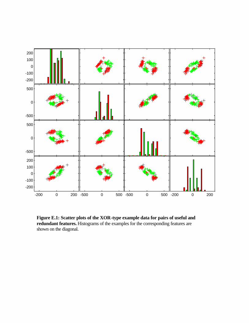
Figure E.1: Scatter plots of the XOR-type example data for pairs of useful and redundant features. Histograms of the examples for the corresponding features are shown on the diagonal.

-200 0 200-500 0 500-500 0 500-200 0 200

-200

-100

0

100

200

-500

0

500

-500

0

500

-200

-100

0

100

200

Figure E.2: Heat map of the XOR-type example data. We show all the coefficients of the data matrix. The intensity indicates the magnitude of the coefficients. The color indicates the sign. In lines, we show the 100 examples drawn (25 per cluster). I columns, we show the 20 features. Only the first 6 ones are relevant: 2 useful, 2 redundant, 2 repeated. The data have been shifted and scaled by column to look “more natural”. The last column shows the target values, with some “flipped” labels.

After adding noise

2 4 6 8 10 12 14 16 18 20

10

20

30

40

50

60

70

80

90

100

Figure E.3: Heat map of the XOR-type example data. This is the same matrix as the

one shown in Figure E.2. However, the examples have been randomly permuted and grouped per class. The features have also been randomly permuted. Consequently, after

normalization, the data looks very uninformative to the eye.

2 4 6 8 10 12 14 16 18 20

10

20

30

40

50

60

70

80

90

100

Figure E.4: Scatter plots of the benchmark data for pairs of useful and redundant features. We can see that the two classes overlap completely in all pairs of features. This is normal because 5 dimensions are needed to separate the data.

2 4 6 8 10 12 14 16 18 20

1000

2000

3000

4000

5000

6000

7000

8000

Figure E.5: Heat map of the benchmark data for the relevant features (useful, redundant, and repeated). We see the clustered structure of the data.


Positive ex. Negative ex. Total Check sum Training set 1000 1000 2000 488026911 Validation set 300 300 600 146425645 Test set 900 900 1800 439236341 All 2200 2200 4400 1073688897 Two additional test sets of the same size were drawn similarly and reserved to be able to test the features selected by the benchmark participants, in case it becomes important to make sure they trained only on those features.


Real variables Random probes Total 20 480 500 All variables are integer. There are no missing values. The data is not sparse. The data was saved as a non-sparse matrix.

7) Results of the run of the lambda method Before the benchmark, we ran some simple methods to determine what an appropriate number of examples should be. The “lambda” method (provided with the sample code) performs rather poorly on this highly non-linear problem (41% error). We used the K-nearest neighbor method, with K=3, with only the 5 useful features. With the 2000 training examples and 2000 test examples, we obtained 10% error. The rule of thumb number_of_test_examples=100/test_errate=100/0.1=1000 makes it likely that 1800 test examples will be sufficient to obtains statistically significant results. The benchmark results confirmed that this was a good (conservative) estimate. Appendix A: Matlab code of the lambda method function idx=lambda_feat_select(X, Y, num) %idx=lambda_feat_select(X, Y, num) % Feature selection method that ranks according to the dot % product with the target vector. Note that this criterion % may not deliver good results if the features are not % centered and normalized with respect to the example distribution. % Isabelle Guyon -- August 2003 -- [email protected] fval=Y'*X; [sval, si]=sort(-fval); idx=si(1:num);

function [W,b]=lambda_classifier(X, Y) %[W,b]=lambda_classifier(X, Y) % This simple but efficient two-class linear classifier % of the type Y_hat=X*W'+b % was invented by Golub et al. % Inputs: % X -- Data matrix of dim (num examples, num features) % Y -- Output matrix of dim (num examples, 1) % Returns: % W -- Weight vector of dim (1, num features) % b -- Bias value. % Isabelle Guyon -- August 2003 -- [email protected] Posidx=find(Y>0); Negidx=find(Y<0); Mu1=mean(X(Posidx,:)); Mu2=mean(X(Negidx,:)); Sigma1=std(X(Posidx,:),1); Sigma2=std(X(Negidx,:),1); W=(Mu1-Mu2)./(Sigma1+Sigma2); B=(Mu1+Mu2)/2; b=-W*B'; Appendix B: Matlab code for generating synthetic data function [XP,YP,ixrp,iyrp, xrp,yrp,all_C,A,B,rf,shift,scale ] = hypercube_data(num_class, num_useful_feat, num_clust_per_class, num_pat_per_cluster, num_redundant_feat, num_repeat_feat, num_useless_feat, class_sep, flip_y, num_repeat_val, rnd, debug, xrp, yrp,all_C,A,B,rf,shift,scale) %[XP,YP,ixrp,iyrp, xrp,yrp,all_C,A,B,rf,shift,scale ] = hypercube_data(num_class 1, num_useful_feat 2, num_clust_per_class 3, num_pat_per_cluster 4, num_redundant_feat 5, num_repeat_feat 6, num_useless_feat 7, class_sep 8, flip_y 9, num_repeat_val 10, rnd 11, debug 12, xrp 13, yrp 14, all_C 15, A 16, B 17,rf 18,shift 19,scale 20) % Draws a pattern recognition problem at random, for a num_class-class problem. % Useful features: % Each class is composed of a number of Gaussian clusters that are on the % vertices of a hypercube in a subspace of dimension num_useful_feat. % N(0,1) is used to draw the examples of independent features for each cluster. % Some covariance is added by multiplying by a random matrix A, % with uniformly distributed random numbers between -1 and 1. % The clusters are then placed on the hypercube vertices. % The hypercube vertices are placed at values +-class_sep. % Redundant features: % Useful features are multiplied by a random matrix B, % with uniformly distributed random numbers between -1 and 1.

% Repeated features: % Drawn randomly from useful and redundant features. % Useless features: % Additional features drawn at random not related to the concept. % Features are then shifted and rescaled randomly to span 3 orders of magnitude. % Random noise is then added to the features according to N(0,.1) to create several replicates. % if flip_y is provided, a random fraction flip_y of labels are randomly exchanged. % -- Aknowledgements: The idea is inspired by the work of Simon Perkins. % Inputs: % num_class -- Number of classes % num_useful_feat -- Number of features initially drawn to explain the concept % num_clust_per_class -- Number of cluster per class % num_pat_per_cluster -- Number of patterns per cluster // all balanced for now, can be generalized to imbalanced classes (can take subset of samples of each class) % num_redundant_feat -- Number of features linearly dependent upon the useful features % num_repeat_feat -- Number of features repeating the previous ones (drawn at random) % num_useless_feat -- Number of features dran at random regardless of class label information % class_sep -- Factor multiplying the hypercube dimension. % flip_y -- Fraction of y labels to be randomly exchanged. % num_repeat_val -- number of times each entry is repeated (modulo some noise). % rnd -- Flag to enable or disable random permutations. % debug -- 0/1 flag. % Returns: % XP -- Matrix (num_pat, num_feat, num_repeat_val) of randomly permuted features % YP -- Vector of 0,1...num_class target class labels (in random order, to be used eventually for clustering) % ixrp -- permutation matrix to be used to restore the original feature order % iyrp -- permutation matrix to be used to restore the original pattern order (class labels of the same class are consecutive % and there are the same number of example per class, before label corruption) % Y=YP(iyrp); X=XP(iyrp,ixrp); % all_C -- A matrix 2^num_useful_feat*num_useful_feat of % hypercube vertices where to place the cluter centers. % A -- Matrix used to correlate the useful features. % B -- Matrix used to create dependent (redundant) features. % rf -- Indices of repeated features. % shift -- Shift applied. % scale -- Scale applied. % Isabelle Guyon -- July 2003 -- [email protected]

if nargin<8, class_sep=1; end if nargin<9, flip_y=0; end if nargin<10, num_repeat_val=1; end if nargin<11, rnd=0; end % disable random permutation if nargin<12, debug=0; end if nargin<13, xrp=[]; end if nargin<14, yrp=[]; end if nargin<15, all_C=[]; end if nargin<16, A={}; end if nargin<17, B=[]; end if nargin<18, rf=[]; end if nargin<19, shift=[]; end if nargin<20, scale=[]; end % Count features and patterns num_feat=num_useful_feat + num_repeat_feat + num_redundant_feat + num_useless_feat; num_pat_per_class=num_pat_per_cluster*num_clust_per_class; num_pat=num_pat_per_class*num_class; X=zeros(num_pat, num_feat); % Attribute class labels y=0:num_class-1; Y=repmat(y, num_pat_per_class, 1); Y=Y(:); % Hypercube design is_XOR=0; if num_useful_feat==2 & num_class==2 & num_clust_per_class==2, is_XOR=1; all_C=[-1 -1; 1 1; 1 -1; -1 1]; % XOR else if isempty(all_C) fprintf('New C\n'); all_C=2*ff2n(num_useful_feat)-1; rndidx=randperm(size(all_C,1)); all_C=all_C(rndidx,:); end end % Draw A if isempty(A) fprintf('New A\n'); for k=1:num_class*num_clust_per_class A{k} = 2*rand(num_useful_feat, num_useful_feat)-1;

end end % Loop over all clusters for k=1:num_class*num_clust_per_class % define the range of patterns of that cluster kmin=(k-1)*num_pat_per_cluster+1; kmax=kmin+num_pat_per_cluster-1; kidx=kmin:kmax; % Draw n features independently at random X(kidx,1:num_useful_feat)=random('norm', 0, 1, num_pat_per_cluster, num_useful_feat); % Multiply by a random matrix to create some co-variance of the features X(kidx,1:num_useful_feat)=X(kidx,1:num_useful_feat)*A{k}; % Shift the center off zero to separate the clusters C=all_C(k,:)*class_sep; X(kidx,1:num_useful_feat) = X(kidx,1:num_useful_feat) + repmat(C, num_pat_per_cluster, 1); end if debug, featdisplay(normalize_data([X(:,1:num_useful_feat),Y])); title('Useful features'); figure; scatterplot(X(:, 1:num_useful_feat), Y); title('Useful features'); end % Create redundant features by multiplying by a random matrix if isempty(B), fprintf('New B\n'); B = 2*rand(num_useful_feat, num_redundant_feat)-1; end X(:,num_useful_feat+1:num_useful_feat+num_redundant_feat)=X(:,1:num_useful_feat)*B; if debug, featdisplay(normalize_data([X(:,1:num_useful_feat+num_redundant_feat),Y])); title('Useful+redundant features'); figure; scatterplot(X(:, 1:num_useful_feat+num_redundant_feat), Y); title('Useful+redundant features'); end % Repeat num_repeat_feat features, chosen at random among useful and redundant feat nf=num_useful_feat+num_redundant_feat; if isempty(rf) fprintf('New rf\n'); rf=round(1+rand(num_repeat_feat,1)*(nf-1)); end X(:,nf+1:nf+num_repeat_feat)=X(:,rf);

if debug, featdisplay(normalize_data([X(:,1:num_useful_feat+num_redundant_feat+num_repeat_feat),Y])); title('Useful+redundant+repeated features'); end % Add useless features : these are uncorrelated with one another, but could be correlated :=) X(:,num_feat-num_useless_feat+1:num_feat)=random('norm', 0, 1, num_pat, num_useless_feat); if debug, featdisplay(normalize_data([X,Y])); title('All features'); end % Add random y label errors num_err_pat = round(num_pat*flip_y); rp=randperm(num_pat); fi=rp(1:num_err_pat); Y(fi)=mod(Y(fi)+round(rand(num_err_pat,1)*(num_class-1)), num_class); if debug, featdisplay(normalize_data([X,Y])); title('All features + flipped labels'); end % Randomly shift and scale if isempty(shift) fprintf('New shift\n'); shift=rand(num_feat,1); end if isempty(scale) fprintf('New scale\n'); scale=1+100*rand(num_feat,1); end X=X+repmat(shift',num_pat,1); X=X.*repmat(scale',num_pat,1); if debug, featdisplay([X,100*normalize_data(Y)]); title('All features + flipped labels + scale shifted'); end % Randomly permute the features and patterns

if isempty(xrp) fprintf('New xrp, yrp\n'); if rnd xrp=randperm(num_feat); yrp=randperm(num_pat); else xrp=1:num_feat; yrp=1:num_pat; end end XP0=X(yrp,xrp); YP=Y(yrp); if debug, [ys,pattidx]=sort(YP); featdisplay(normalize_data([XP0(pattidx,:),YP(pattidx)])); title('After permutation and data normalization'); end % Create inverse random indices ixrp(xrp)=1:num_feat; iyrp(yrp)=1:num_pat; % Create several replicates by adding a little bit of random noise XP=zeros(num_pat, num_feat, num_repeat_val); for k=1:num_repeat_val N=random('norm', 0, .1*sqrt(num_repeat_val), num_pat, num_feat); XP(:,:,k)=XP0.*(1+N); end if debug, featdisplay(normalize_data([XP(pattidx,:),YP(pattidx)])); title('After adding noise'); end

design of experiments for the nips 2003 variable selection benchmark isabelle guyon...

Documents