Feature selection and causal discovery

fundamentals and applications

Isabelle Guyon isabelle@clopinet.com

Feature Selection

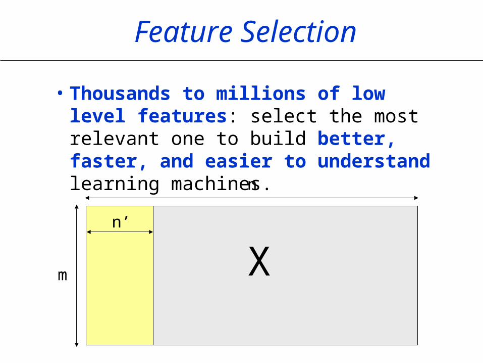
• Thousands to millions of low level features: select the most relevant one to build better, faster, and easier to understand learning machines.

X

n

m

n’

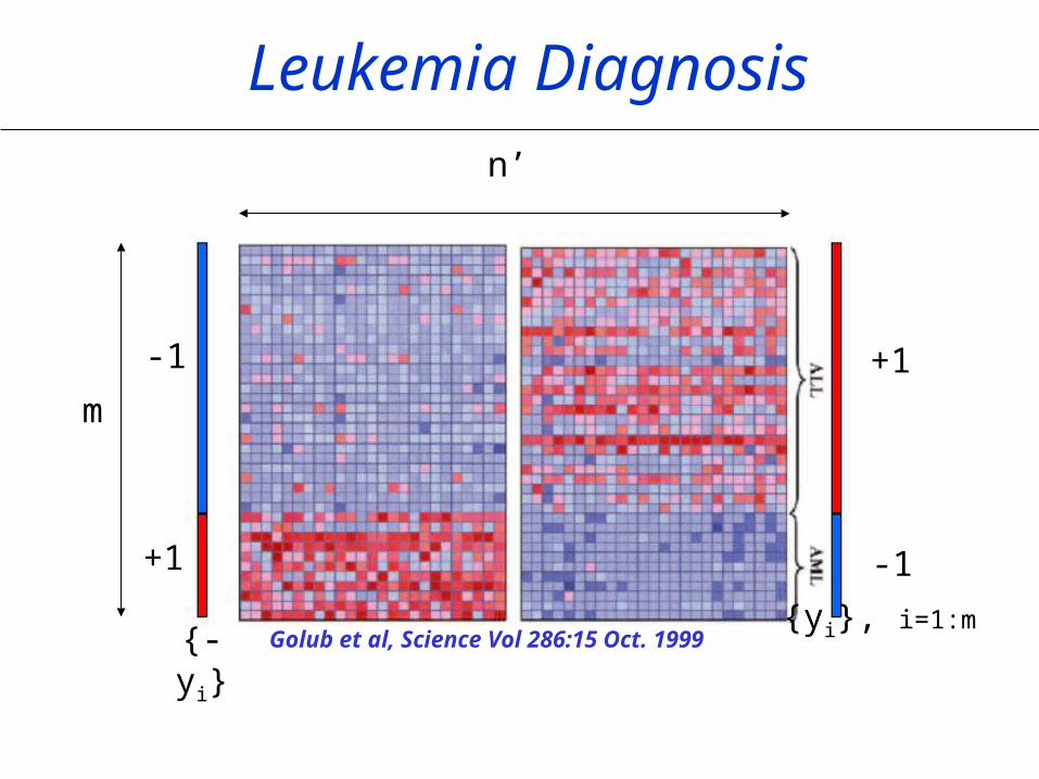
Leukemia Diagnosis

Golub et al, Science Vol 286:15 Oct. 1999

+1

-1

-1

+1

m

n’

{yi}, i=1:m{-yi}

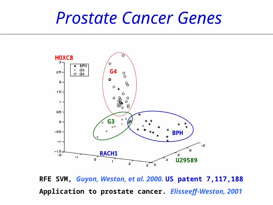
RFE SVM, Guyon, Weston, et al. 2000. US patent 7,117,188

Application to prostate cancer. Elisseeff-Weston, 2001

U29589

HOXC8

RACH1

BPH

G4

G3

Prostate Cancer Genes

Differenciation of 14 tumors. Ramaswamy et al, PNAS, 2001

RFE SVM for cancer diagnosis

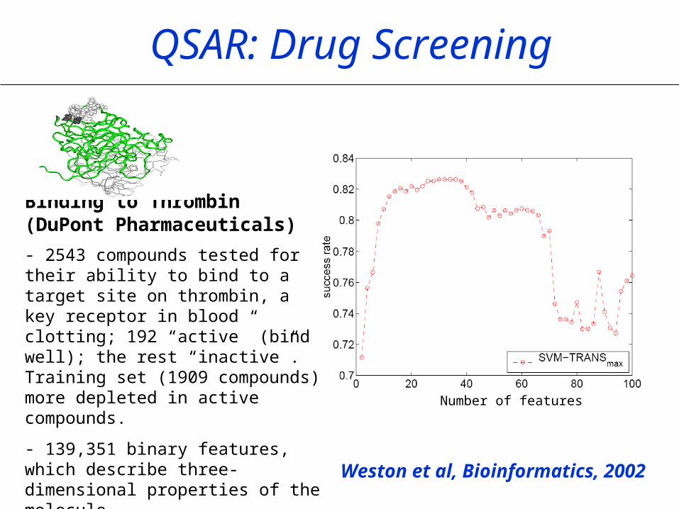
QSAR: Drug Screening

Binding to Thrombin(DuPont Pharmaceuticals)

- 2543 compounds tested for their ability to bind to a target site on thrombin, a key receptor in blood clotting; 192 “active” (bind well); the rest “inactive”. Training set (1909 compounds) more depleted in active compounds.

- 139,351 binary features, which describe three-dimensional properties of the molecule. Weston et al, Bioinformatics, 2002

Number of features

Text Filtering

Bekkerman et al, JMLR, 2003

Top 3 words of some categories:• Alt.atheism: atheism, atheists, morality• Comp.graphics: image, jpeg, graphics• Sci.space: space, nasa, orbit• Soc.religion.christian: god, church, sin• Talk.politics.mideast: israel, armenian, turkish• Talk.religion.misc: jesus, god, jehovah

Reuters: 21578 news wire, 114 semantic categories.

20 newsgroups: 19997 articles, 20 categories.

WebKB: 8282 web pages, 7 categories.

Bag-of-words: >100000 features.

Face Recognition

Relief:

Simba:

100 500 1000

• Male/female classification•1450 images (1000 train, 450 test), 5100 features (images 60x85 pixels)

Navot-Bachrach-Tishby, ICML 2004

Nomenclature

• Univariate method: considers one variable (feature) at a time.

• Multivariate method: considers subsets of variables (features) together.

• Filter method: ranks features or feature subsets independently of the predictor (classifier).

• Wrapper method: uses a classifier to assess features or feature subsets.

Univariate Filter

Methods

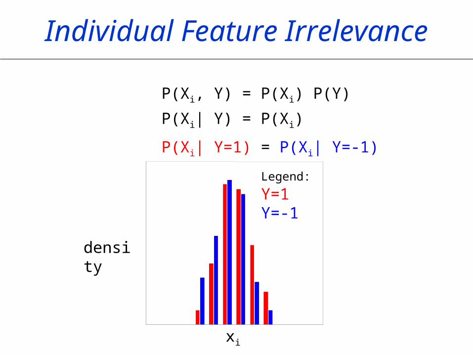
Individual Feature Irrelevance

P(Xi, Y) = P(Xi) P(Y)

P(Xi| Y) = P(Xi)

P(Xi| Y=1) = P(Xi| Y=-1)

xi

density

Legend: Y=1 Y=-1

S2N

-1

- +

- +

Golub et al, Science Vol 286:15 Oct. 1999

+1

-1

-1

+1

m

{-yi} {yi}

S2N = |+ - -|+ + -

S2N R x y

after “standardization” x (x-x)/x

Univariate Dependence

• Independence:

P(X, Y) = P(X) P(Y)

• Measure of dependence:

MI(X, Y) = P(X,Y) log dX dY

= KL( P(X,Y) || P(X)P(Y) )

P(X,Y)

P(X)P(Y)

A choice of feature selection ranking methods depending on the nature of:

• the variables and the target (binary, categorical, continuous)

• the problem (dependencies between variables, linear/non-linear relationships between variables and target)

• the available data (number of examples and number of variables, noise in data)

• the available tabulated statistics.

Other criteria ( chap. 3)

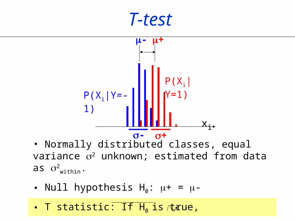
T-test

• Normally distributed classes, equal variance 2 unknown; estimated from data as 2

within.

• Null hypothesis H0: + = -

• T statistic: If H0 is true,

t= (+ - -)/(withinm++1/m-Studentm++m--d.f.

-1

- +

- +

P(Xi|Y=-1)

P(Xi|Y=1)

xi

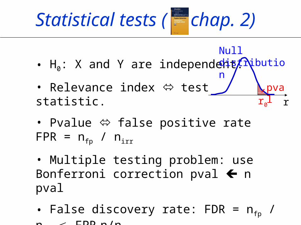
• H0: X and Y are independent.

• Relevance index test statistic.

• Pvalue false positive rate FPR = nfp / nirr

• Multiple testing problem: use Bonferroni correction pval n pval

• False discovery rate: FDR = nfp / nsc FPR n/nsc

• Probe method: FPR nsp/np

pvalr0 r

Null distribution

Statistical tests ( chap. 2)

Multivariate Methods

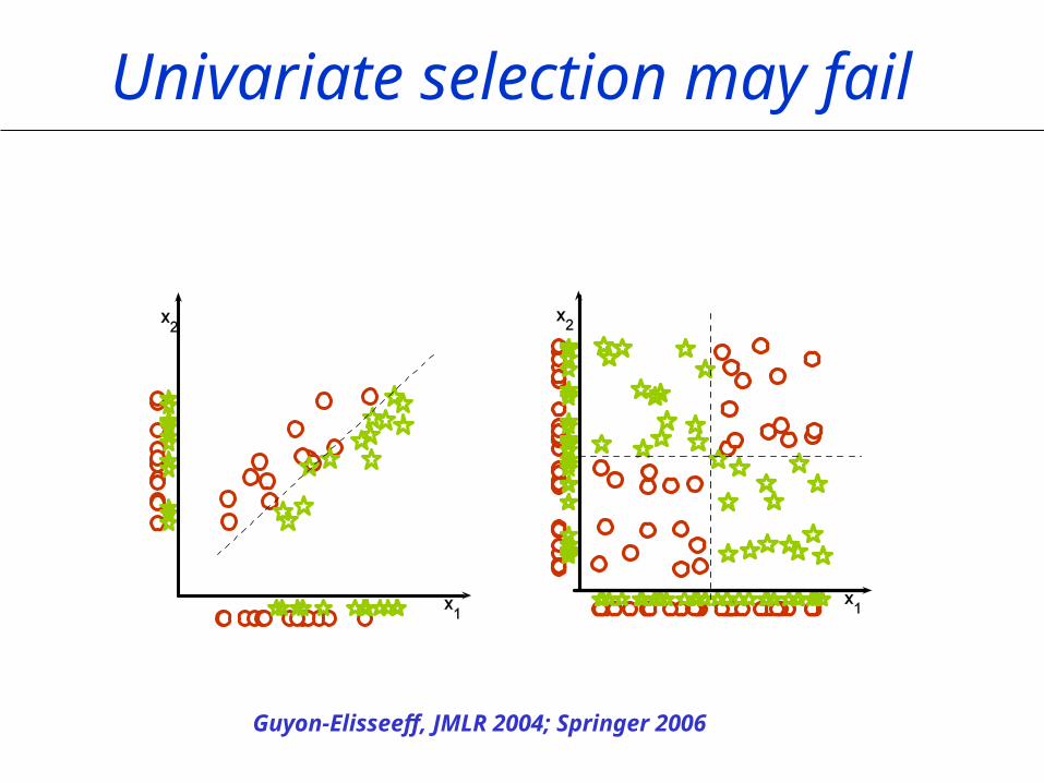
Univariate selection may fail

Guyon-Elisseeff, JMLR 2004; Springer 2006

Filters,Wrappers, andEmbedded methods

All features FilterFeature subset Predictor

All features

Wrapper

Multiple Feature subsets

Predictor

All featuresEmbedded

method

Feature subset

Predictor

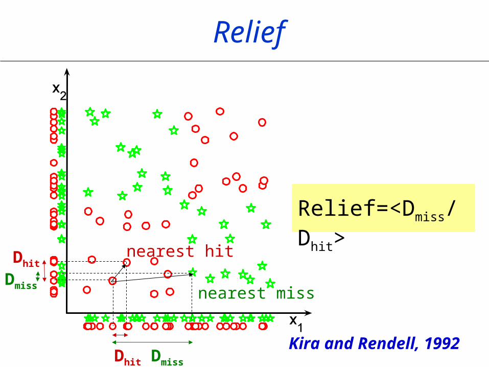
Relief

nearest hit

nearest miss

Dhit Dmiss

Relief=<Dmiss/Dhit>

Dhit

Dmiss

Kira and Rendell, 1992

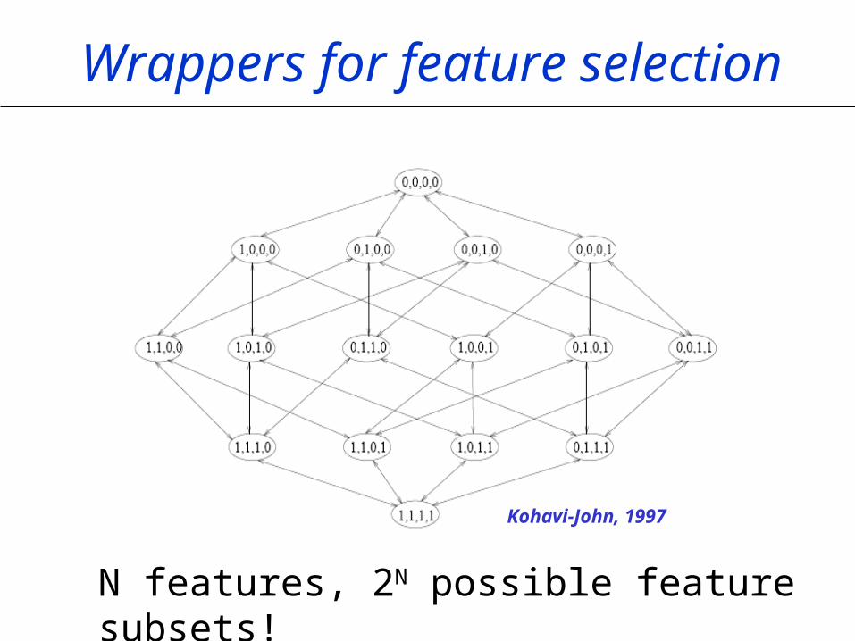
Wrappers for feature selection

N features, 2N possible feature subsets!

Kohavi-John, 1997

• Exhaustive search.• Simulated annealing, genetic algorithms.• Beam search: keep k best path at each step. • Greedy search: forward selection or backward

elimination.• PTA(l,r): plus l , take away r – at each step, run

SFS l times then SBS r times.• Floating search (SFFS and SBFS): One step of

SFS (resp. SBS), then SBS (resp. SFS) as long as we find better subsets than those of the same size obtained so far. Any time, if a better subset of the same size was already found, switch abruptly.

n-kg

Search Strategies ( chap. 4)

Feature subset assessment

1) For each feature subset, train predictor on training data.

2) Select the feature subset, which performs best on validation data.– Repeat and average if you

want to reduce variance (cross-validation).

3) Test on test data.

N variables/features

M s

ampl

es

m1

m2

m3

Split data into 3 sets:training, validation, and test set.

Statistical tests

Single feature ranking

Cross validation

Performance bounds

Nested subset,forward selection/ backward elimination

Heuristic orstochastic search

Exhaustive search

Single featurerelevance

Relevancein context

Feature subset relevance

Performance learning machine

Search

Criterion

Ass

essm

ent

Statistical tests

Single feature ranking

Cross validation

Performance bounds

Nested subset,forward selection/ backward elimination

Heuristic orstochastic search

Exhaustive search

Single featurerelevance

Relevancein context

Feature subset relevance

Performance learning machine

Three “Ingredients”

Statistical tests

Single feature ranking

Cross validation

Performance bounds

Nested subset,forward selection/ backward elimination

Heuristic orstochastic search

Exhaustive search

Single featurerelevance

Relevancein context

Feature subset relevance

Performance learning machine

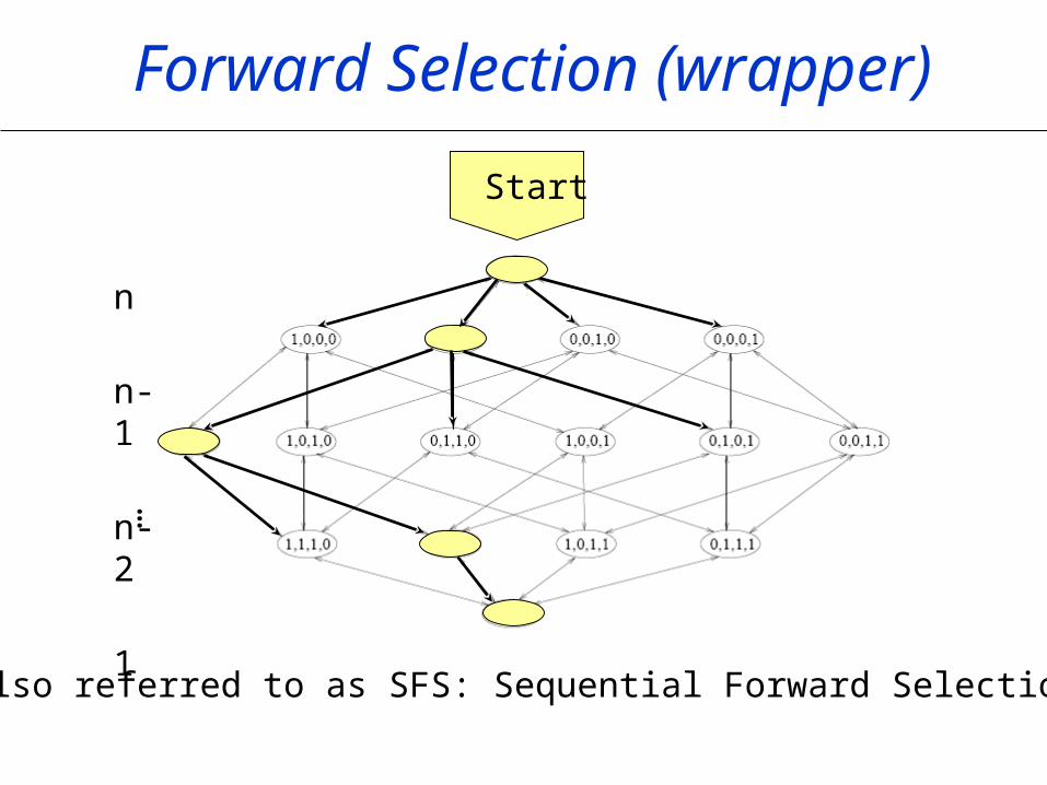
Forward Selection (wrapper)

n

n-1

n-2

1

…

Start

Also referred to as SFS: Sequential Forward Selection

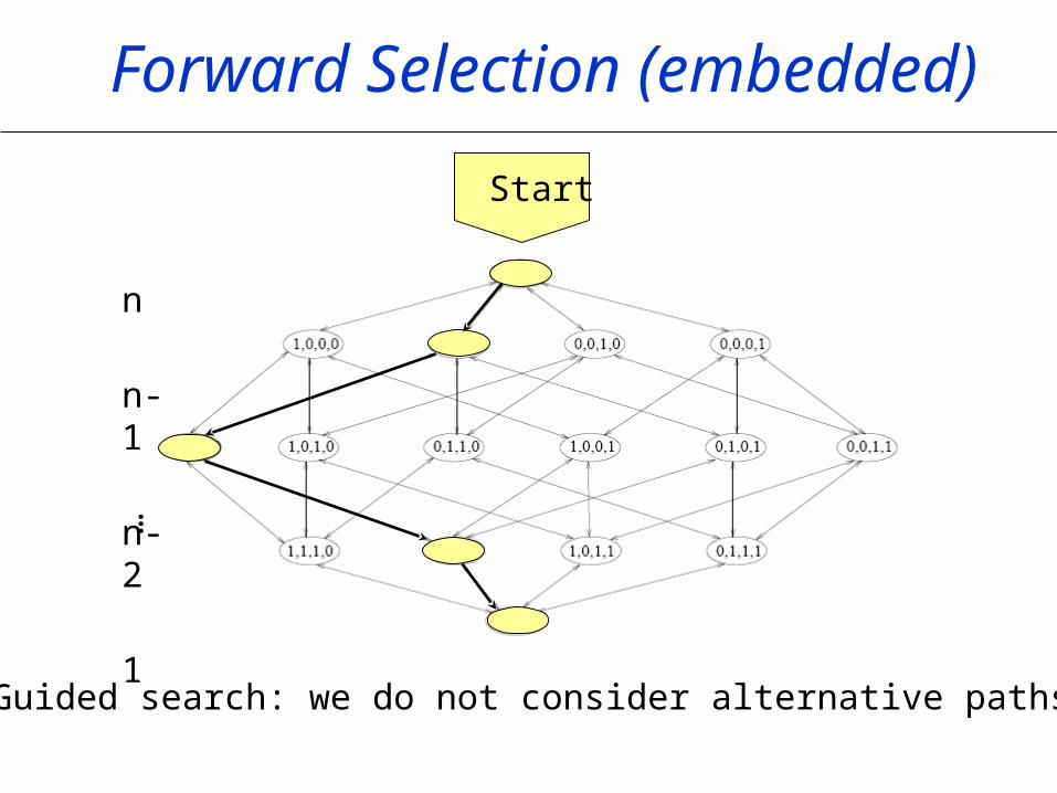
Guided search: we do not consider alternative paths.

Forward Selection (embedded)

…

Start

n

n-1

n-2

1

Forward Selection with GS

• Select a first feature Xν(1)with maximum cosine with the target cos(xi, y)=x.y/||x|| ||y||

• For each remaining feature Xi

– Project Xi and the target Y on the null space of the features already selected

– Compute the cosine of Xi with the target in the projection

• Select the feature Xν(k)with maximum cosine with the target in the projection.

Embedded method for the linear least square predictor

Stoppiglia, 2002. Gram-Schmidt orthogonalization.

Forward Selection w. Trees

• Tree classifiers,

like CART (Breiman, 1984) or C4.5 (Quinlan, 1993)

At each step, choose the feature that

“reduces entropy” most. Work

towards “node purity”.

All the data

f1

f2

Choose f1

Choose f2

Backward Elimination (wrapper)

1

n-2

n-1

n

…

Start

Also referred to as SBS: Sequential Backward Selection

Backward Elimination (embedded)

…

Start

1

n-2

n-1

n

Backward Elimination: RFE

Start with all the features.• Train a learning machine f on the current subset

of features by minimizing a risk functional J[f].• For each (remaining) feature Xi, estimate,

without retraining f, the change in J[f] resulting from the removal of Xi.

• Remove the feature Xν(k) that results in improving or least degrading J.

Embedded method for SVM, kernel methods, neural nets.

RFE-SVM, Guyon, Weston, et al, 2002. US patent 7,117,188

Scaling Factors

Idea: Transform a discrete space into a continuous space.

• Discrete indicators of feature presence: i {0, 1}

• Continuous scaling factors: i IR

=[1, 2, 3, 4]

Now we can do gradient descent!

Learning with scaling factors

X={xij}

n

m y ={yj}

• Many learning algorithms are cast into a minimization of some regularized functional:

Empirical errorRegularization

capacity control

Formalism ( chap. 5)

Next few slides: André Elisseeff

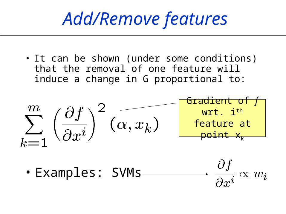
Add/Remove features

• It can be shown (under some conditions) that the removal of one feature will induce a change in G proportional to:

• Examples: SVMs

Gradient of f wrt. ith feature at point xk

Recursive Feature Elimination

Minimize estimate of

R(,) wrt.

Minimize the estimate R(,) wrt. and under a constraint that

only limited number of

features must be selected

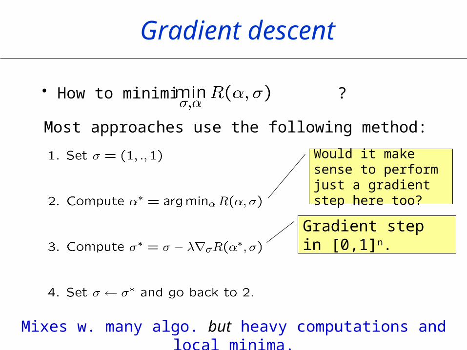
Gradient descent

• How to minimize ?

Most approaches use the following method:

Gradient step in [0,1]n.

Would it make sense to perform just a gradient step here too?

Mixes w. many algo. but heavy computations and local minima.

Minimization of a sparsity function

• Minimize the number of features used

• Replace by another objective function:

– l1 norm:

– Differentiable function:

• Optimize jointly with the primary objective (good prediction of a target).

The l1 SVM

• The version of the SVM where ||w||2 is replace by the l1 norm i |wi| can be considered as an embedded method:– Only a limited number of weights will be

non zero (tend to remove redundant features)

– Difference from the regular SVM where redundant features are all included (non zero weights)

Bi et al 2003, Zhu et al, 2003

Ridge regression

w1

w2

w*

J = ||w||22 + 1/ ||w-w*||2

Mechanical interpretationw2

J = ||w||22 + ||w-w*||2

w*

w1

w1

w2

w*

J = ||w||1 + 1/ ||w-w*||2

Lasso Tibshirani, 1996

• Replace the regularizer ||w||2 by the l0 norm

• Further replace by i log( + |wi|)

• Boils down to the following multiplicative update algorithm:

The l0 SVM

Weston et al, 2003

Embedded method - summary

• Embedded methods are a good inspiration to design new feature selection techniques for your own algorithms:– Find a functional that represents your prior knowledge about

what a good model is.– Add the weights into the functional and make sure it’s

either differentiable or you can perform a sensitivity analysis efficiently

– Optimize alternatively according to and – Use early stopping (validation set) or your own stopping

criterion to stop and select the subset of features

• Embedded methods are therefore not too far from wrapper techniques and can be extended to multiclass, regression, etc…

Causality

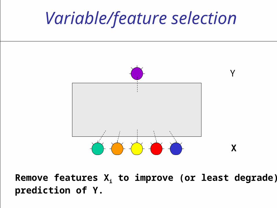
Variable/feature selection

Remove features Xi to improve (or least degrade) prediction of Y.

X

Y

What can go wrong?

Guyon-Aliferis-Elisseeff, 2007

X2 X1

180 190 200 210 220 230 240 250 260

20

40

60

80

100

120

What can go wrong?

20 40 60 80 100

8

10

12

14

16

20

40

60

80

100

X2 X1

X1

X

2

X2 X1

180 190 200 210 220 230 240 250 260

20

40

60

80

100

120

What can go wrong?

Guyon-Aliferis-Elisseeff, 2007

X2 Y

X1

Y

X1X2

X

Y

Causal feature selection

Uncover causal relationships between Xi and Y.

Y

Coughing

Allergy

Smoking

Anxiety

Genetic factor1

Hormonal factor

Metastasis(b)

Other cancers

Lung cancerGenetic factor2

Tar in lungs

Bio-marker2

Biomarker1

Systematic noise

Causal feature relevance

Formalism:Causal Bayesian networks

• Bayesian network:– Graph with random variables X1, X2, …Xn

as nodes.– Dependencies represented by edges.– Allow us to compute P(X1, X2, …Xn) as

i P( Xi | Parents(Xi) ).

– Edge directions have no meaning.

• Causal Bayesian network: egde directions indicate causality.

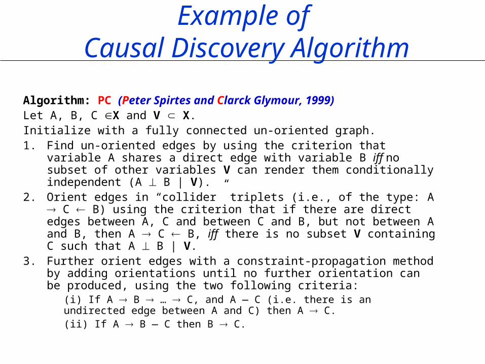
Example of Causal Discovery Algorithm

Algorithm: PC (Peter Spirtes and Clarck Glymour, 1999)Let A, B, C X and V X. Initialize with a fully connected un-oriented graph.1. Find un-oriented edges by using the criterion that variable A

shares a direct edge with variable B iff no subset of other variables V can render them conditionally independent (A B | V).

2. Orient edges in “collider” triplets (i.e., of the type: A C B) using the criterion that if there are direct edges between A, C and between C and B, but not between A and B, then A C B, iff there is no subset V containing C such that A B | V.

3. Further orient edges with a constraint-propagation method by adding orientations until no further orientation can be produced, using the two following criteria:

(i) If A B … C, and A — C (i.e. there is an undirected edge between A and C) then A C. (ii) If A B — C then B C.

Computational and statistical complexity

Computing the full causal graph poses:• Computational challenges (intractable for large numbers of

variables)• Statistical challenges (difficulty of estimation of conditional

probabilities for many var. w. few samples).

Compromise:• Develop algorithms with good average- case

performance, tractable for many real-life datasets.• Abandon learning the full causal graph and instead

develop methods that learn a local neighborhood.• Abandon learning the fully oriented causal graph and

instead develop methods that learn unoriented graphs.

Target Y

A prototypical MB algo: HITON

Aliferis-Tsamardinos-Statnikov, 2003)

Target Y

1 – Identify variables with direct edges to the target (parent/children)

Aliferis-Tsamardinos-Statnikov, 2003)

Target Y

Aliferis-Tsamardinos-Statnikov, 2003)

A

B Iteration 1: add A

Iteration 2: add B

Iteration 3: remove A because A Y | B

etc.

A

A B

B

1 – Identify variables with direct edges to the target (parent/children)

Target Y

Aliferis-Tsamardinos-Statnikov, 2003)

2 – Repeat algorithm for parents and children of Y (get depth two relatives)

Target Y

Aliferis-Tsamardinos-Statnikov, 2003)

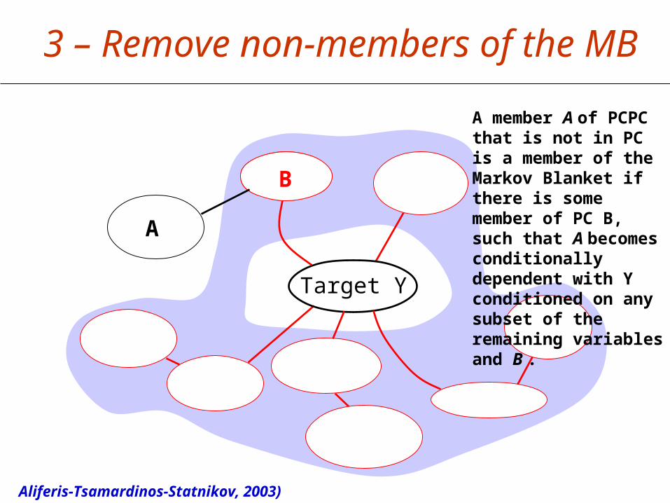
3 – Remove non-members of the MB

A member A of PCPC that is not in PC is a member of the Markov Blanket if there is some member of PC B, such that A becomes conditionally dependent with Y conditioned on any subset of the remaining variables and B .

A

B

Wrapping up

Complexity of Feature Selection

Method Number of subsets tried

Complexity C

Exhaustive search wrapper

2N N

Nested subsets Feature ranking

N(N+1)/2 or N

log N

Generalization_error Validation_error + (C/m2)

m2: number of validation examples, N: total number of features,n: feature subset size.

With high probability:

n

Error

Try to keep C of the order of m2.

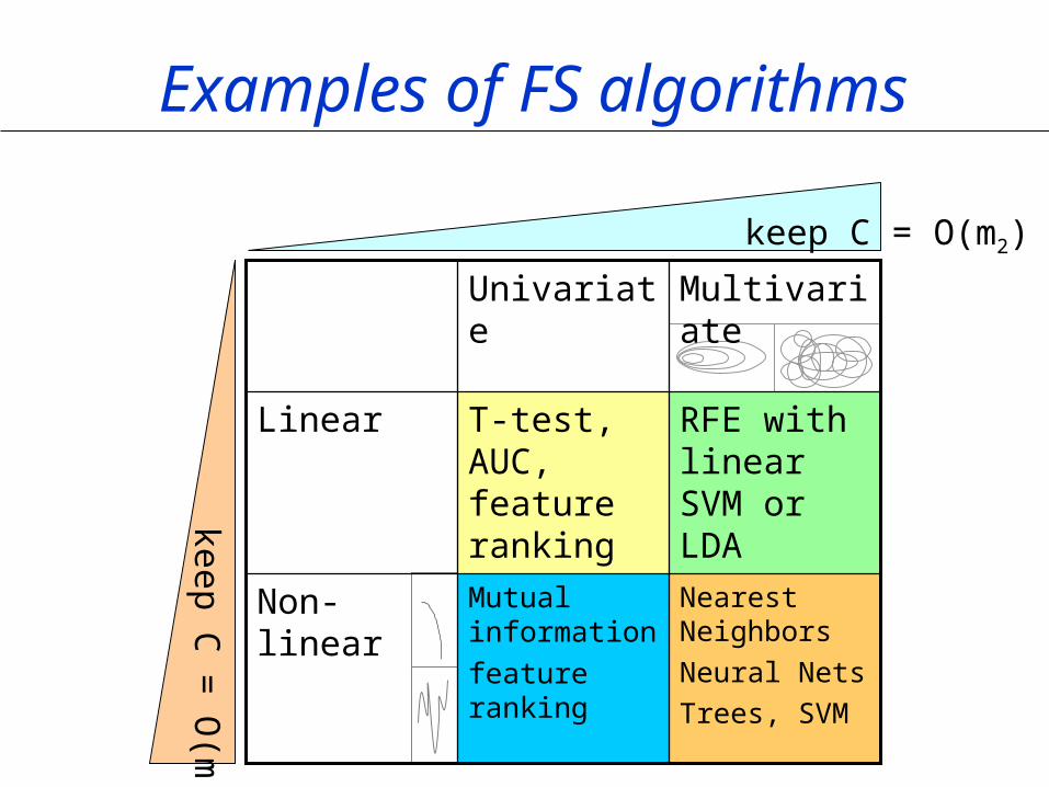
Examples of FS algorithms

keep C = O(m2)

keep C =

O(m

1)

Nearest Neighbors

Neural Nets

Trees, SVM

Mutual information

feature ranking

Non-linear

RFE with linear SVM or LDA

T-test, AUC, feature ranking

Linear

MultivariateUnivariate

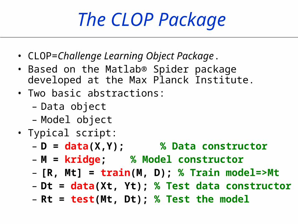
The CLOP Package

• CLOP=Challenge Learning Object Package.• Based on the Matlab® Spider package developed at the

Max Planck Institute.• Two basic abstractions:

– Data object– Model object

• Typical script:– D = data(X,Y); % Data constructor– M = kridge; % Model constructor– [R, Mt] = train(M, D); % Train model=>Mt– Dt = data(Xt, Yt); % Test data constructor– Rt = test(Mt, Dt); % Test the model

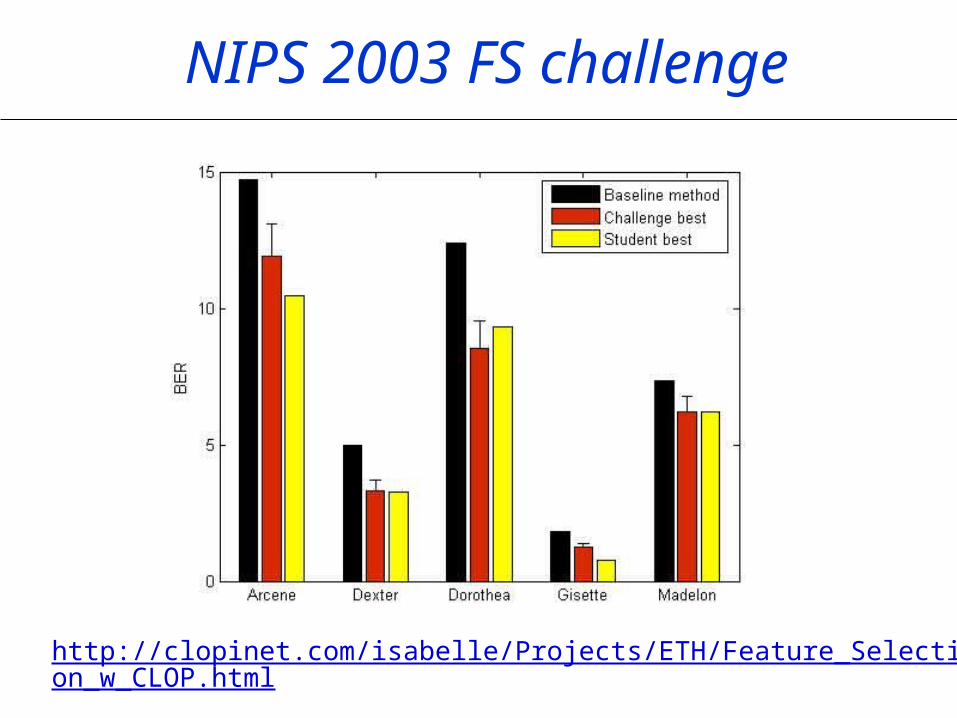
NIPS 2003 FS challenge

http://clopinet.com/isabelle/Projects/ETH/Feature_Selection_w_CLOP.html

Conclusion

• Feature selection focuses on uncovering subsets of variables X1, X2,

… predictive of the target Y. • Multivariate feature selection is in

principle more powerful than univariate feature selection, but not always in practice.

• Taking a closer look at the type of dependencies in terms of causal relationships may help refining the notion of variable relevance.

1) Feature Extraction, Foundations and ApplicationsI. Guyon et al, Eds.Springer, 2006.http://clopinet.com/fextract-book

2) Causal feature selectionI. Guyon, C. Aliferis, A. ElisseeffTo appear in “Computational Methods of Feature Selection”, Huan Liu and Hiroshi Motoda Eds., Chapman and Hall/CRC Press, 2007.http://clopinet.com/isabelle/Papers/causalFS.pdf

Acknowledgements and references