DEPARTMENT OF COMMUNICATIONS ENGINEERINGDEGREE PROGRAMME IN WIRELESS COMMUNICATIONS ENGINEERING

DESIGN OF APPLICATION-SPECIFICSIGNAL PROCESSORS FOR ITERATIVETURBO DECODER

AuthorShahriar Shahabuddin

Supervisorprof. Markku Juntti

Accepted / 2012

Grade

Shahabuddin S. (2012) Design of application-specific signal processors for itera-tive turbo decoder. University of Oulu, Department of Communications Engineering,Master’s Degree Programme in Wireless Communications Engineering, Master’s the-sis, 67 p.

ABSTRACT

In order to meet the requirement of high data rates for the next generationtelecommunication systems, the efficient implementation of receiver algorithmsis essential. On the other hand, the rapid development of technology moti-vates the investigation of programmable implementations to shorten developmenttimes. This thesis describes the design of programmable turbo decoder as anapplication-specific signal processor (ASSP).

Two turbo decoder processors with Transport Triggered Architecture (TTA)are designed. The first TTA processor is designed with very basic function unitsand is able to support one suboptimal maximum a posteriori (MAP) algorithm forthe soft-input soft-output (SISO) decoders. The second TTA procesor is designedwith special function units to accelerate the computationally intensive parts ofthe turbo decoding algorithm. The processor architecture is designed in such amanner that it can be programmed to support four different suboptimal formsof the MAP algorithm. The design enables the device to change the suboptimalalgorithms according to the bit error rate (BER) performance requirement. Thethroughputs of the processor for different algorithms are compared to one an-other. The max-log-MAP outperforms the other suboptimal algorithms in termsof latency.

Quadratic permutation polynomial (QPP) interleaver is used for contentionfree memory access and to make the processors Long Term Evolution (LTE) com-pliant. Several optimization techniques to enable real time processing on pro-grammable platforms are introduced. The first processor achieves 10.12 Mbpsthroughput with a single iteration for a clock frequency of 200 MHz. The secondprocessor achieves 31.21 Mbps throughput with a single iteration for the max-log-MAP algorithm for the same clock frequency.

Keywords: ASSP, TTA, MAP, SISO, BER, QPP, LTE.

Shahabuddin S. (2012) Sovelluskontaisen signaaliprosessorin suunnittelu iterati-iviselle turbo dekooderille. Oulun yliopisto, Tietoliikennetekniikan osasto, Master’sDegree Programme in Wireless Communications Engineering, Diplomityö, 67 s.

TIIVISTELMÄ

Tehokkaat vastaanotinalgoritmitoteutukset ovat merkittävässä asemassa kun ha-lutaan saavuttaa tulevaisuuden tietoliikennejärjestelmien korkeat data nopeudet.Teknologiakehitys motivoi tutkimaan ohjelmoitavia toteutuksia tuotteiden markki-noille saamisen nopeuttamiseksi. Tämä diplomityö kuvaa turbo dekooderin suun-nittelun ohjelmoitavalle sovelluskohtaiselle signaaliprosessorille.

Työssä on suunniteltu kaksi siirtoliipaisuarkkitehtuuriin (TTA) perustuvaaprosessoria turbo dekooderille. Ensimmäinen toteutus sisältää yleiskäyttöisiä las-kentayksiköitä ja tukee alioptimaalista MAP-algoritmia pehmeän päätöksen de-kooderille. Toinen sovellus sisältää erikoislaskentayksiköitä, jotka kiihdyttävätturbo dekooderin laskennallisesti raskaita osia ja näin parantavat suorituskykyä.Prosessoriarkkitehtuuri on suunniteltu siten, että se tukee neljää eri versiotaalioptimaalisesta MAP-algoritmista. Ohjelmoitava ratkaisu mahdollistaa algo-ritmin vaihtamisen bittivirhesuhteen mukaan. Työssä on vertailtu prosessorinsuorituskykyä eri algoritmeille. Max-log-MAP algoritmi saavuttaa parhaimmanlatenssin verrattuna muihin tutkittuihin alioptimaalisiin algoritmeihin.

Tässä työssä on käytetty QPP-lomittelijaa (quadratic polynomial permuta-tion) muistiosoitusristiriitojen poistamiseksi sekä tekemään toteutuksesta LTE(Long Term Evolution) yhteensopivan. Toteutuksessa on esitetty useita optimoin-timenetelmiä reaaliaikavaatimusten saavuttamiseksi. Ensimmäinen prosessorito-teutus saavuttaa 10,12 Mbps suorituskyvyn yhdellä turbo dekooderi-iteraatiolla,kun prosessorin kellotaajuus on 200 MHz. Vastaavasti toinen prosessoritoteutussaavuttaa 31,21 Mbps suorituskyvyn kun käytetään max-log-MAP algoritmia.

Avainsanat: TTA, MAP, QPP, LTE.

TABLE OF CONTENTS

ABSTRACT

TIIVISTELMÄ

TABLE OF CONTENTS

PREFACE

SYMBOLS AND ABBREVIATIONS

1. INTRODUCTION 10

2. MIMO SYSTEM 122.1. MIMO Transmission . . . . . . . . . . . . . . . . . . . . . . . . . . 122.2. MIMO-OFDM . . . . . . . . . . . . . . . . . . . . . . . . . . . . . 132.3. MIMO Detection . . . . . . . . . . . . . . . . . . . . . . . . . . . . 14

3. TURBO CODEC 173.1. Historical Development . . . . . . . . . . . . . . . . . . . . . . . . . 173.2. Turbo Encoding . . . . . . . . . . . . . . . . . . . . . . . . . . . . . 183.3. Turbo Decoding . . . . . . . . . . . . . . . . . . . . . . . . . . . . . 20

3.3.1. Turbo Decoder without Feedback . . . . . . . . . . . . . . . 203.3.2. Iterative Turbo Decoder . . . . . . . . . . . . . . . . . . . . 21

3.4. Decoding Algorithm . . . . . . . . . . . . . . . . . . . . . . . . . . 223.4.1. MAP Algorithm . . . . . . . . . . . . . . . . . . . . . . . . 243.4.2. Suboptimal MAP Algorithms . . . . . . . . . . . . . . . . . 29

3.5. Interleavers . . . . . . . . . . . . . . . . . . . . . . . . . . . . . . . 303.5.1. Types of Interleavers . . . . . . . . . . . . . . . . . . . . . . 303.5.2. Contention Free Property of Interleaver . . . . . . . . . . . . 313.5.3. Quadratic Permutation Polynomial Interleaver . . . . . . . . . 32

4. ASSP DESIGN METHODOLOGY 334.1. Embedded System Design Methods . . . . . . . . . . . . . . . . . . 334.2. From RISC to TTA . . . . . . . . . . . . . . . . . . . . . . . . . . . 344.3. Transport Triggered Architectures . . . . . . . . . . . . . . . . . . . 354.4. TTA based Codesign Environment . . . . . . . . . . . . . . . . . . . 374.5. ASSP Design using TCE . . . . . . . . . . . . . . . . . . . . . . . . 38

5. DESIGN 405.1. Decoder Requirements . . . . . . . . . . . . . . . . . . . . . . . . . 405.2. Design in High Level Language . . . . . . . . . . . . . . . . . . . . 405.3. Algorithm Optimization . . . . . . . . . . . . . . . . . . . . . . . . . 425.4. Code Optimization . . . . . . . . . . . . . . . . . . . . . . . . . . . 465.5. Hardware Design . . . . . . . . . . . . . . . . . . . . . . . . . . . . 475.6. Processor Architecture with General Function Units . . . . . . . . . . 48

5.7. Processor Architecture with Special Function Units . . . . . . . . . . 495.7.1. METRIC Special Function Unit . . . . . . . . . . . . . . . . 515.7.2. MAX7 Special Function Unit . . . . . . . . . . . . . . . . . 52

6. RESULTS 546.1. Simulation Results . . . . . . . . . . . . . . . . . . . . . . . . . . . 546.2. Processor Architecture with General Function Units . . . . . . . . . . 566.3. Processor Architecture with Special Function Unit . . . . . . . . . . . 576.4. Comparison . . . . . . . . . . . . . . . . . . . . . . . . . . . . . . . 59

7. DISCUSSION 61

8. SUMMARY 63

9. REFERENCES 64

PREFACE

The research work presented in this thesis has been carried out as part of the Co-operative MIMO Techniques for Cellular System Evolution (CoMIT) project in De-partment of Communications Engineering and Centre for Wireless Communications(CWC) at the University of Oulu, Finland. I would like to gratefully acknowledgethe Finnish Funding Agency for Technology and Innovation (Tekes), Renesas MobileEurope, Nokia Siemens Networks, Elektrobit and Xilinx for providing the financialsupport for this project.

I would like to gratefully acknowledge my supervisor professor Markku Juntti, forproviding me the opportunity to work in CoMIT project. His enthusiastic support andcriticism helped to me to complete my thesis work successfully. Special thanks goes toDr. Janne Janhunen for his patient guidance throughout my thesis work. I would liketo thank the second examiner professor Olli Silven from Center for Machine VisionResearch (CMV), University of Oulu, for his helpful comments.

I would also like to thank Jarkko Huusko, Dr. Janne Lehtomäki, Essi Suikkanen,Uditha Lakmal Wijewardhana from CWC, Dr. Perttu Salmela from Qualcomm, Dr.Jani Boutellier and Teemu Nyländen from CMV, University of Oulu, for their sug-gestions and help for my thesis. I would like to thank the whole CWC staff for thenice working environment. I would like to thank my friends and seniors, includingHelal Chowdhury, Hassan Malik, Amanullah Ghazi, Ijaz Ahmad, Nouman Bashir, Dr.Zaheer Khan, Khawer Shafqat, Muhammad Zeeshan Asghar, Gagan Mazed for theirmental support and help throughout the thesis.

I would like to thank my parents most, for their love and encouragement throughoutmy studies. Finally, I am grateful to the Almighty Allah for the completion of themaster’s thesis.

SYMBOLS AND ABBREVIATIONS

∥ · ∥2F squared Frobenius norm(·)† pseudoinverse(·)H Hermitian conjugate(·)T matrix transposeα forward metricβ backward metricγ branch metricσ2 varianceΩ symbol alphabetΩr real-valued symbol alphabetfc(·) correction functionIm· imaginary part of argumentL(·) log-likelihood ratioln natural logarithmP (·) probabilityRe· real part of argument

C set of complex numbersD2

LMMSE LMMSE detectorR set of real numbersZ set of integer numbers

c transmitted code wordsH channel matrixHr real valued-channel matrixHS channel matrix for subcarrier SnS noise vectorr received code wordsR0 set of transitions for input 0R1 set of transitions for input 1Rxx symbol covariance matrixRnn noise covariance matrixu data wordsx transmitted symbol vectorxr real-valued transmitted symbol vectorxS transmitted symbol vector for subcarrier Sx estimate of transmitted signalx maximum likelihood estimatey received signal vectoryr real-valued received signal vectoryS received signal vector for subcarrier S

a parameter for linear-log-MAP Jacobi algorithmm number of bits in data wordC0 sphere radius

M number of receive antennasMI number of windowsn number of bits in code wordN number of transmit antennasNI number of LLR valuesNQ block length of QPP interleaverR coding rates present states′ previous stateT parameter for constant-log-MAP Jacobi algorithmWI window size

kbps kilobits per secondkmph kilometer per hourMbps megabits per secondMHz megahertz

3GPP the third generation partnership projectADD additionADF architecture definition fileALU arithmetic logic unitAPP a posteriori probabilityARP almost regular permutationASIC application-specific integrated circuitASIP application-specific instruction-set processorASSP application-specific signal processorAWGN Additive white Gaussian noiseBCH Bose and Chaudhuri and HocquenghemBER bit error rateCISC complex instruction-set computingDMC discrete memoryless channelDRP Dithered relative primeDSP digital signal processorEQ equalFEC forward error correctionFFT fast Fourier transformFIFO first-in first-outFPGA field programmable gate arrayFU function unitGCU global control unitGPP general purpose processorIDF implementation definition fileIFFT inverse fast Fourier transformIIR infinite impulse responseILP instruction level parallelismISI intersymbol interferenceLDPC low-density parity-check

LLR log likelihood ratioLMMSE linear minimum mean square errorLSD list sphere detectorLSU load-store unitLTE long term evolutionLUT look-up tableMAP maximum a posterioriMIMO multiple-input multiple-outputML maximum likelihoodOFDM orthogonal frequency division multiplexingPSK phase shift keyingQAM quadrature amplitude modulationQPP quadratic polynomial permutationRF register fileRISC reduced instruction-set computingRS Reed-SolomonRSC recursive systematic convolutionalRTL register transfer levelSFU special function unitSHL shift leftSHR shift rightSIMD single instruction multiple dataSIMD single-instruction multiple-dataSINR signal-to-noise-plus-interference ratioSISO soft-input soft-outputSOVA soft-output Viterbi algorithmSPMD single-program multiple-dataSTBC space time block codesSUB subtractionSVD singular value decompositionTCE TTA Codesign EnvironmentTCM trellis coded modulationTPEF TTA program exchange formatTTA transport triggered architectureUMTS universal mobile telecommunication systemVBLAST vertical-Bell Laboratories layered space-timeVHDL VHSIC hardware description languageVLIW very long instruction wordZF zero-forcing

1. INTRODUCTION

In 1948, Shannon published his landmark paper, where he proved that it is possible toachieve channel capacity even with low transmitting power and nearly free from errorsby using certain coding schemes [1]. Scientists could not find this perfect codingscheme for the next forty five years. In 1993, Berrou et al . proposed the turbo codingscheme which outperformed all the coding schemes invented previously [2].

The turbo coding scheme has been adopted as the error correcting scheme in mostof the important communication standards. As an example, the turbo coding schemehas been adopted for the air interface standard Long Term Evolution (LTE), that hasbeen defined by the 3rd Generation Partnership Project (3GPP) [3]. As LTE is beingdeployed by the major carriers worldwide, the importance of turbo coding scheme isalso increasing.

The turbo decoder is one of the most complex parts of wireless receivers. The algo-rithms needed for the component decoders, which are part of the whole turbo decoder,are complex. The data dependencies make this algorithms more difficult to implementin hardware platforms. Another bottleneck is the iterative nature of the turbo decoder,which makes the implementation with low latency difficult.

As the turbo decoding is computationally intensive, the designers favour the hard-ware implementation. A drawback is that a hardware implementation is fixed and evena slight change in design is not possible later. For the rapidly changing telecommuni-cation standards, an inflexible implementation is not a very good choice. The relativelyslow development time of a hardware implementation is also a bottleneck.

The decoding algorithm for the component decoder is not specified by 3GPP. Dif-ferent suboptimal algorithms have been used for the turbo decoding and new solutionswith less complexity are still being invented frequently. The software based implemen-tations of turbo decoder in a general purpose processor or in a digital signal processorprovide the required flexibility to support multistandard solutions, but requires a care-ful design to achieve the target throughput. It is very difficult to meet the LTE data ratethrough software implementation alone.

A flexible implementation simplifies the necessary support for different subopti-mal algorithms and different interleaving methods. However, it is very difficult toachieve high throughput without hardware implementations. Programmable acceler-ators, which enable software-hardware co-design might be an attractive solution toovercome these bottlenecks. The design of software and hardware together to grindout the best performance and ensure programmability is not a straightforward task.The designer needs a very efficient tool, which can be used to design the processoreasily for a particular application.

In this thesis, the design of processors based on the Transport Triggered Architec-ture (TTA) for a flexible turbo decoder is investigated. TTA is a very good processortemplate for a programmable application-specific signal processor (ASSP). The TTAbased codesign environment (TCE) tool is used. It enables the designer to write theapplication with high level language and design the target processor in a graphical userinterface at the same time [4].

A turbo decoder based on TTA was implemented by Salmela et al . [5]. The through-put of the processor was comparable with turbo decoders based on a pure hardwaredesign. However, the processor was not flexible to support other algorithms and was

11

rather similar to the hardware implementations. The interleaver of the processor wasnot presented according to the 3GPP LTE standard.

The key target of the turbo decoder processor design in this thesis is flexibility. Thequadratic permutation polynomial (QPP) interleaving pattern is used for the interleaverblock. The comparison with different suboptimal algorithms for component decodersis also presented.

The thesis is organized in the following way. In Chapter 2, an overview of themultiple-input multiple-output (MIMO) systems and different detection algorithm isdiscussed briefly. In Chapter 3, the turbo encoder and decoder structures are described.The decoding algorithm is presented after that. Finally, the interleaver and the de-interleaver are explained. Chapter 4 gives an overview of the ASSP design method-ology using the TTA processor design tool, TCE. Chapter 5 describes the designedprocessor architectures in detail. The simplification of the decoding algorithm is alsogiven in this chapter. Chapter 6 describes the evaluation of the design and Chapter 7presents the future work. The thesis is summarized in Chapter 8.

12

2. MIMO SYSTEM

A general overview of the MIMO systems is presented in this chapter. The subsec-tions include the explanation of general MIMO transmission and MIMO detection.A short description of orthogonal frequency-division multiplexing (OFDM) combinedwith MIMO is also provided in another subsection.

2.1. MIMO Transmission

Instead of using a single antenna for transmission or reception, several antennas can beutilized in transceivers to improve system capacity. These systems are called MIMOsystems. MIMO systems increase data throughput and link range without additionalbandwidth. The reasons for the improvement in performance are array gain, diversitygain, spatial multiplexing gain and interference reduction. Due to these benefits, theMIMO systems have been adopted as the transmission strategy for the upcoming stan-dards like IEEE 802.11n, IEEE 802.16e and LTE and it has the potential to be used inwider range of standards for communications [6] [7].

The MIMO techniques can be categorized in three ways. The first type which in-cludes techniques like delay diversity or space time block codes (STBC) aims to im-prove the power efficiency by maximizing spatial diversity [8]. The second type in-creases the capacity by following a layered approach. One example of such type ofMIMO systems is the vertical-Bell Laboratories layered space time (V-BLAST) archi-tecture [9]. The third type uses the singular value decomposition (SVD) to decomposethe channel matrix and use these decomposed matrices as pre and post filters [10].

Despite having all these benefits, the MIMO systems have some drawbacks, too.The use of multiple antennas increases the complexity of multi-dimensional signalprocessing. The need of multiple antennas increase the cost of equipment also. Thesystem design also becomes more expensive [11].

Consider N transmit antennas are sending binary data over the MIMO channel. Thedata bits are encoded in the transmitter with some techniques like convolutional codingor turbo coding. The encoded bits are sent to the modulator where the bits are arrangedas symbol vectors. In the receiver the opposite operations such as demodulation anddecoding takes place, trying to detect the original binary data.

Figure 1. Simple example of MIMO systems.

Let us consider these operations mathematically. Suppose the MIMO system con-sists of N transmit antennas, which are sending data over the channel and M receive

13

antennas which are receiving transmitted bits from the channel as shown in Figure 1.The modulation scheme that is used here is quadrature amplitude modulation with theassumption N ≥M . The received signal is composed of the multiplication of the com-plex channel matrix and transmitted symbol vector with the additional white Gaussiannoise caused the by the channel. The received signal y can be represented as

yS = HSxS + nS, (1)

where S is the number of subcarriers, yS ∈ CM is the received signal vector, xS ∈ CN

is the transmit symbol vector and nS ∈ CM is the noise vector with independentand complex zero mean Gaussian elements with equal variance σ2 for both real andimaginary parts. The channel matrix HS ∈ CN×M consists of channel coefficients insuch a way that hn,m is the channel coefficient from the nth transmit antenna and mthreceive antenna [12]. The channel matrix HS can be expressed as

HS =

h1,1 h1,2 . . . h1,N

h2,1 h2,2 . . . h2,N...

......

...hM,1 hM,2 . . . hM,N

. (2)

Any complex linear MIMO system model can be redesigned to an equivalent realsystem model by splitting the real and imaginary parts. The equivalent real systemmodel can be rewritten as

yr = Hrxr + nr, (3)

where the real valued channel matrix for two transmit and two receive antennas is

Hr =

[ReH −ImHImH ReH

]∈ R2N×2M , (4)

and the real valued vectors are defined by

yr = [ReyTImyT]T ∈ R2M , (5)

xr = [RexTImxT]T ∈ Z2N , (6)

nr = [RenTImnT]T ∈ R2M , (7)

where Re· and Im· denote the real and imaginary parts, respectively. The realvalued symbol alphabet is now ΩΩΩr = Z.

2.2. MIMO-OFDM

The MIMO system described above boost the capacity and in this higher rate datatransmission the multipath characteristics causes the channel to become frequency se-lective. Thus, multipath characteristics restrict the increase of transmission rate. Thesolution is to divide the high speed data stream in to several narrowband data stream.

14

The mechanism is called OFDM. The OFDM transforms a frequency selective MIMOchannel in to a set of parallel frequency flat subchannels [13].

The subcarriers are orthogonal to one another in time domain. On the other hand, thesignal spectra corresponding to these subcarriers overlap in frequency. Thus, OFDMcan make the efficient use of frequency. In a frequency-selective channel, a cyclic-prefix is typically used to make the signal robust to frequency selectivity.

One of the major disadvantages is the OFDM time domain signal having a relativelylarge peak-to-average ratio. In addition, OFDM is sensitive to inter-channel inter-ference and frequency and time synchronization errors. A block diagram of MIMOOFDM transmitter is given in Figure 2 [11].

Figure 2. Block diagram of a MIMO-OFDM transmitter.

While MIMO introduces channel diversity for space, OFDM can efficiently makethe best use of the available bandwidth. The combination of two powerful techniqueslike MIMO and OFDM has become one of the most promising broadband wirelessschemes.

2.3. MIMO Detection

The function of the MIMO detector is to estimate the transmitted signal vector and tofeed the soft output to the decoder. The detector needs an estimation of the channeland the received signal as input. A block diagram of the MIMO OFDM detector isprovided in Figure 3 [11].

Detection algorithms can be divided in two categories. The hard output detectionalgorithms will choose only one of the alphabets from the whole transmitted alphabetand the other alphabets will be discarded. Maximum likelihood (ML) detectors are oneof the optimal hard decision detectors. ML detector is not used in practical cases be-cause of the complexity. The second type of detector is soft output detectors. The softoutput algorithms calculate reliability values instead of selecting one of the alphabets.Maximum a posteriori (MAP) detector is one of the optimum detectors.

The optimal detection algorithms like ML and MAP are complex. Therefore, somesuboptimal detectors like linear minimum mean square error (LMMSE) or zero-forcing(ZF) are used instead of the optimal detectors.

15

Figure 3. Block diagram of a MIMO OFDM detector.

ML Detector

The ML detector calculates the Euclidean distances between received signal y andlattice points Hx and selects the closest lattice point. To find the closest lattice point,the ML detector selects that particular lattice point for which the Euclidean distance isminimum, i.e.,

xML = arg minx∈ΩΩΩM

∥ y −Hx ∥22 . (8)

MAP Detector

The MAP detector is the optimal soft input soft output detector. The MAP algorithmfinds the probability of the transmitted bit being either +1 or −1. This is equivalent offinding the a posteriori probability.

LMMSE Detector

The LMMSE detector minimizes the mean square error (MSE) between the transmittedsignal vector x and the soft output vector x. The LMMSE detector can be expressedas

D2LMMSE = min

WE∥ x−WHy ∥2F, (9)

where x ∈ CN is the transmitted signal vector, W ∈ CN×M is the LMMSE coefficientmatrix and y ∈ CM . Using Wiener solution we can find the coefficient matrix as

W = (HRxxHH +Rnn)

−1HRxx, (10)

where H ∈ CN×M denotes the channel matrix, Rxx ∈ CN×M is the symbol covariancematrix and Rnn ∈ CN×M is the noise covariance matrix in (10). In the end, the outputof the LMMSE detector can be calculated as

x = WHy. (11)

16

ZF Detector

In ZF detector, the data streams are separated and each stream is decoded indepen-dently. The ZF estimation can be expressed as

x = (HHH)-1Hx = H†x, (12)

where H is the channel matrix and (·) denotes the pseudoinverse.

K-Best LSD Detector

The sphere detection (SD) algorithms solve the ML problems by only considering thelattice points inside a sphere of a given radius. The condition for a lattice point lyinginside the sphere is

∥ y −Hx ∥2≤ C0. (13)

List sphere detection (LSD) is used to approximate the MAP detection algorithm. Alist of candidates and their Euclidean distances are used to calculate the soft outputsfor the decoder. The K-best algorithm is a breadth search algorithm, which keeps theK number of nodes with smallest Euclidean distances at each step. A node is notexpanded when the partial Euclidean distance (PED) is greater than C [14].

17

3. TURBO CODEC

The turbo coding scheme is described in this chapter. The chapter is divided in fivesections. The historical development of the turbo code is described in the first section.The turbo encoder and decoder are described in next two sections. The algorithm usedfor decoding the component decoders are given after that. The last section describesthe basic ideas related to interleavers, their usage, different types of interleavers andrelative benefits of them.

3.1. Historical Development

Communication channels suffer from channel noise due to the imperfections of thereal life channels. The received data contains error when transmitted over a noisychannel. Channel coding or forward error correction (FEC) is a technique used todetect and correct these errors caused by the noisy or unreliable channels during datatransmission. The idea is to add systematic redundancy to the transmitted signal, whichcan be used for error detection and correction without retransmitting. The drawback ofadding redundant bits is higher forward channel bandwidth. Redundancy is added inthe form of parity bits, which are calculated from the original bits with special channelcoding algorithms.

The utility of the coding schemes was demonstrated in [1]. According to Shannon,the communication channel has a maximum rate for reliable data transmission calledchannel capacity. As mentioned earlier, Shannon showed the possibility to achievethe channel capacity even with low transmitting power and nearly free from errors byusing certain coding schemes. Shannon did not answer the question which code wouldachieve this. Shannon suggested infinitely long and random codewords to achievethe channel capacity. However, it is not practical to use long and random codewordsbecause of the increasing computational complexity [1].

Coding experts focused on practical sides and using parity bit started to make rea-sonably good codes. The idea was to use an extra bit or parity bit with the originalcodeword which could be later used to detect errors. However, this basic scheme couldnot correct errors. It could only be used to detect if any error occurred. To correcterrors, the coding scheme needed to use more parity bits. Though the coding schemeswere giving fairly good results using more parity bits, it was still nowhere near to thetheoretical performance that was suggested by Shannon. The use of more parity bitsmade the codwords longer and decoding became more complex. After the surprisingresults shown by Shannon, the coding theory field attracted plenty of attention and in-tensive research efforts have been made in order to find the perfect coding solution.Due to these extensive research the channel coding schemes developed a lot and thedevelopment came up with Hamming codes [15], convolutional codes and Viterbi algo-rithm [16], Bose and Chaudhuri and Hocquenghem (BCH) code [17], Reed-Solomoncode (RS) [18], trellis coded modulation (TCM) [19] etc., which are fairly good codes.The gap between the transmitted power needed for these codes and the transmittedpower that should be necessary according to Shannon was not satisfactory yet. Thesecodes needed much more power than that should be necessary and still the perfect codewas not found [20].

18

About 45 years after Shannon’s pioneering work, Berrou et al . invented a codingscheme that would provide nearly error free communication. They called this codingscheme turbo coding [2]. The main features of this coding scheme are parallel con-catenated coding, recursive convolutional encoders, pseudo-random interleavers anditerative decoding scheme. The complexity was reduced by splitting the complexityinto more manageable components. The heart of the turbo decoding is the iterativeprocess where the decoders take advantage of each other by exchanging information.

The coding scheme proposed by Berrou et al . reported significant improvementover the already existing convolutional codes. The gap between the Shannon limit andimplementation practice was only 0.7 dB while the convolutional codes left 3 dB gapsbetween the theory and practice [20].

3.2. Turbo Encoding

Convolutional Codes

The convolutional codes are widely used and adopted for different communicationstandards. Convolutional codes were first introduced by Elias in 1955 [21]. Convolu-tional codes are linear codes, which usually operate as good as block codes. As anybinary code, convolutional codes add redundant bits which are used later to correct er-rors. A rate m/n convolutional encoder takes the m-bit information symbols as inputsequence and produces n-bit symbol (n > m) output sequence. The convolutionalencoders can be represented as a finite state machine. The operation of the encodercan be described by state or trellis diagrams. A trellis diagram is a presentation of thestate transitions of the convolutional encoders as a function of time. The convolutionalencoders are used as the basic building blocks of a turbo encoder.

Recursive systematic convolutional (RSC) codes are a kind of infinite impulse re-sponse (IIR) convolutional codes. The term systematic is used because one of theoutput bits is directly using the input data streams and sending it directly over thechannel [22].

Figure 4. Diagram of a RSC encoder.

19

The term recursive is used because previously encoded information bits are contin-uously fed back to the encoders input. The non-systematic convolutional (NSC) codegenerates a binary rate RSC code, if a feedback loop is introduced with the NSC codeas shown in Figure 4. RSC codes result in better bit error rate (BER) performancethan the NSC at higher code rates and it is true for any signal-to-noise ratio. RSCcodes do not modify the output weight distribution of the codewords for the same codegenerators [22].

Turbo Encoder

The turbo encoder consists of parallel concatenation of two RSC encoders. The inputbits go through the first RSC encoder and create the first parity bits. The input bits, afterbeing scrambled by the interleaver, go through the second RSC encoder and create thesecond parity bits. The input bits are also transmitted through the channel directly. Inother words, the input bits are systematically transmitted through the channel. Everyinput bit creates three output bits, one information bit which is transmitted directly andtwo parity bits.

It is not mandatory that the two RSC encoders have to be identical. The codingrates R1 and R2 for two component encoders should satisfy the R1 ≥ R2. The overallcoding rate of the turbo encoder can be stated as

1

R=

1

R1

+1

R2

− 1. (14)

Parallel concatenation enables the encoders to run at the same clock unlike serialconcatenation. This is one of the issues which simplifies for turbo encoder circuitdesign.

RSC codes are convolutional codes, but turbo code is a block code. The reason isthe interleaver divides the input stream into blocks. This is also one of the reasonsfor the delays associated with the turbo codes. The interleaver forms long block codefrom small memory convolutional code and the decoder has to wait for the interleavedsequence from the interleaver [2].

3GPP LTE Turbo Encoder

The turbo encoding scheme of the LTE and LTE-A standard defined by the 3GPPcontains a parallel concatenated convolutional code with two eight-state constituentencoders and one QPP interleaver [3]. A block diagram of the turbo encoder is givenin Figure 5. The code rate for LTE turbo coding scheme is assumed to be 1/3. Theencoder should encode a m-bit data word to a corresponding code word of n = 3m.There should be 12 bits used for the trellis termination. The first three tail bits shallbe used to terminate the first constituent encoder while the second constituent encoderis disabled. The last three tail bits shall be used to terminate the second constituentencoder while the first constituent encoder is disabled. These 12 bits are used to setthe states of the registers back to zero. The block sizes are also defined which shouldbe in between 40 to 6,144.

20

Figure 5. Block diagram of a turbo encoder.

3.3. Turbo Decoding

3.3.1. Turbo Decoder without Feedback

The structure of the turbo decoder is given in Figure 6. It consists of two soft-inputsoft-output (SISO) decoders and interleaver in the similar fashion to the encoder. Thesoft decisions are real number estimates depending on the clipping. Clipping limits asignal once it exceeds a certain value. Let us assume that the soft decisions are realnumber values between [−5, +5]. Any output with a value of −5 will be a certain 0and any output with a value of +5 will be a certain 1. Any output with a value between−4 to 4 will be uncertain and more iterations will be needed.

The soft estimates are log-likelihood ratios (LLR). As the names suggests, LLR isthe logarithm of the ratio of two probabilities. For example, if a single data bit uk issent at time k the LLR can be denoted by

L(uk) = ln(P (uk = 1)

P (uk = 0)), (15)

where P (uk = 1) denotes that the probability of the transmitted bit is 1 and P (uk = 0)denotes the probability of the transmitted bit is 0.

There are two SISO decoders corresponding to the two RSC encoders in turbo en-coder block. The inputs of the turbo decoder come from the soft detector, which pro-duces the LLRs for the systematic bits and parity bits. The LLRs of the systematic bitand first parity bits goes to the first SISO decoder. The SISO decoder produces softoutputs based on the LLRs. The soft outputs are used in the second SISO decoder asthe additional information.

The inputs of the second SISO decoders are LLRs coming from the systematic bits,second parity bits and the output of the first SISO decoder. The original bit stream are

21

Figure 6. Block diagram of a turbo decoder.

scrambled by the interleaver and encoded through the second RSC encoder to createthe second parity bits. Therefore, the LLRs of the systematic bits have to be scrambledwith the same interleaving pattern used at the encoder. Similarly, the soft outputs com-ing from the first SISO decoder should be scrambled also with the same interleavingpattern which would be used as a priori values for the second SISO decoder. Thesecond SISO decoder will also produce the soft outputs, but this time its output wouldbe better than the first SISO decoder because it is using the outputs of the first SISOdecoder as additional information. The output of the second SISO decoder would beused as final output and this is the construction of a general turbo decoder [2].

3.3.2. Iterative Turbo Decoder

The heart of whole turbo coding is the iterative decoding procedure. In the earliersection the turbo decoder without a feedback loop is described. When a feedback

Figure 7. Block diagram of an iterative turbo decoder.

22

loop is introduced, the output of the second SISO decoder does not produce the hardoutputs immediately. Its soft output is used again in the first SISO decoder. Thesesoft outputs from the second SISO decoder would be subtracted from the a prioriinformation to get the extrinsic information. The extrinsic information denotes theextra information got from the second SISO decoder. The extrinsic information wouldbe descrambled again with similar deinterleaving pattern and will be sent back to thefirst SISO decoder. A block diagram of this scenario is provided in Figure 7. Afterdescrambling, the extrinsic information would be used as the a priori values for thefirst SISO decoder. This time the first SISO decoder also has three inputs, which arethe LLRs coming from the systematic bits, the first parity bit and extrinsic informationcoming from the second SISO decoder. The whole process continues in a similarfashion in cycles. One pass by both the first and the second SISO decoder is referred toas full iteration. On the other hand, the operation performed by a single SISO decodercan be referred to as half iteration. The a priori values are set to zero before startingthe iterations. Normally, six to eight turbo iterations are used [2].

3.4. Decoding Algorithm

SISO decoder can be defined as a decoder, which takes a priori information as theinput and produces a posteriori information as the output. The three inputs of theSISO decoders are systematic information, parity information and a priori informa-tion. The inputs are shown in Figure 8. The output of the SISO decoder is a posterioriinformation as mentioned in the definition.

Figure 8. Inputs and output of a SISO decoder.

The two component encoders of the turbo encoder use convolutional encoding. TheSISO decoding algorithm, which is used for each of the component decoder of theturbo encoder, decodes the convolutional codes. The Viterbi algorithm and MAP aretwo widely used SISO decoding algorithms to determine the state sequence of theconvolutional encoder. A classification of the trellis based algorithms is given in Figure9.

When the received observation sequences are given, the Viterbi algorithm finds themost probable state sequences out of all the states of the trellis encoder. The state se-quences determined by the Viterbi algorithm form a connected path through the trellis[16].

23

The MAP algorithm is also known as BCJR algorithm according to the name ofthe four inventors, Bahl, Cocke, Jelinek and Raviv [23]. In contrast to Viterbi algo-rithm, the MAP algorithm determines each state transition without considering all thereceived observation sequence of the trellis.

The Viterbi algorithm has found universal application to decode the convolutionalcode since its introduction in 1967. The reason lies in the fact that Viterbi algorithmis the optimal decoding method which minimizes the probability of sequence errorfor convolutional code. However, Viterbi algorithm is not suitable for turbo decod-ing because of being a hard-output algorithm. Hagenauer and Hoeher introduced themodification in Viterbi Algorithm, which is known as the soft-output Viterbi algorithm(SOVA). The SOVA is a SISO algorithm, which retains the information related all thetrellis states and provides the probabilities of the states being either one or zero. Thisinformation determines the reliability of the bits which is a direct contrast to the orig-inal hard-output viterbi algorithm. As a result, SOVA is comparatively more complexthan the hard-output Viterbi, but the performance gains realized for the soft outputcompensates for this additional complexity.

In 1996, an improved SOVA was developed to mitigate the inherent bias problemof SOVA. As the name suggests, the improved SOVA is an improved version of theoriginal SOVA. In improved SOVA, the output is multiplied by a normalizing con-stant, which can be derived from the mean and variance of the output. As a result theperformance improves with the price of a small increased complexity.

Figure 9. Classification of trellis based algorithms.

The Viterbi algorithm is not able to produce the a posteriori probability of eachdecoded bit. That is why Viterbi algorithm is not suitable for turbo decoding in spiteof being the optimal decoding method for the convolutional encoding. The MAP algo-rithm was introduced in 1974 to estimate the a posteriori probabilities for a finite-stateMarkov process.

The MAP algorithm finds probabilities of each states of a trellis diagram in theforward direction, as well as in the backward direction. Therefore, the path of theMAP algorithm need not be connected in the trellis like the Viterbi algorithm.

The MAP algorithm needs to be modified to use for turbo decoding. For the RSCcodes, the recursive nature needs to be taken care of. On the other hand, the original

24

MAP algorithm is very complex to be used for the turbo decoding. Therefore, the sub-optimal forms of MAP algorithms, like the log-MAP and max-log-MAP are used forpractical decoders. The log-MAP provides better performance, but more complex thanthe max-log-MAP algorithm. Two other forms of MAP algorithms are also used, whichare constant-log-MAP and linear-log-MAP. These two algorithms are more complexthan max-log-MAP, but less complex than log-MAP. In the next sections we will de-scribe the MAP algorithm in mathematical terms.

3.4.1. MAP Algorithm

Let us consider, a convolutional encoder produces a sequence of K number n-bitcodewords c = c1, c2, c3, . . . , cK from the same number of m-bit datawords u =u1, u2, u2, . . . , uK . If the encoder is generating a codeword ck for an input of uk atany time k, the a priori values of uk can be expressed as

L(uk) = ln(P (uk = 1)

P (uk = 0)). (16)

The probability of the correct decision becomes higher if the a priori probability isalso high [23]. The sign of the bit uk can also be estimated from the magnitude of thea priori probability.

The sequence of the codewards c is transmitted over the channel. These codewordsare received as a sequence of real numbers r = r1, r2, r3, . . . , rK in the receiver sidedue to the imperfection of the channel. The task of the MAP algorithm is to determinethe original datawords u based on the received sequence of r.

As stated before, the MAP algorithm estimates the probabilities of the original bits,which were sent over the channel, being one or zero if the received symbol sequenceis given. This can be called as finding the a posteriori log likelihood ratio.

The MAP algorithm computes a posteriori log likelihood ratio L(uk|r) as

L(uk) = ln(P (uk = 1|r)P (uk = 0|r)

). (17)

The term posteriori is used, because the computations have to be done after r is known.These a posteriori probabilities denote the probabilities of the correctness of the deci-sion, i.e., the confidence level for the decisions. The higher the amplitude of the valuethe more the decision can be trusted.

In Figure 10, a trellis section of an eight state convolutional encoder is shown. Thissection only shows three time instances and the two transitions in between. There areeight small circles in each time instances representing eight states of each time instant.Sixteen transitions can take place in between two time instances and these transitionsare shown by the lines connected between the states. The dashed line represents thetransition caused by an input zero and the dotted line represents the transitions for aninput one. There can be two transitions from a single state and these two transitionsdepend on whether the input bit is zero or one. Therefore, the probabilities of an inputbit being zero or one could be also expressed as the probability of the transitions. Inthat case the right side of (17) can be expressed as

P (uk = 0|r) =∑R0

P (s′, s|r), (18)

25

Figure 10. Trellis of a convolutional encoder with three time instances.

P (uk = 1|r) =∑R1

P (s′, s|r), (19)

where R0 and R1 contain the sets of transitions for uk = 0 or uk = 1 and s′ and srepresents the previous state and present state, respectively.

It is known from the Bayes’ rule that,

P (A,B) = P (B|A)p(A) = P (A|B)P (B)

⇒ P (B|A) = P (A|B)p(B)

P (A).

(20)

If A does not depend on B,

P (B|A) = P (A|B)P (B). (21)

Equation (17) can be re-written as

L(uk) = ln(P (uk = 1|r)P (uk = 0|r)

)

= ln

∑R1

P (s′, s|r)∑R0

P (s′, s|r)

= ln

∑R1

P (s′, s, r)/P (r)∑R0

P (s′, s, r)/P (r)

= ln

∑R1

P (s′, s, r)∑R0

P (s′, s, r).

(22)

26

The received sequence r1, r2, r3, . . . , rK can be divided in three parts. At any timeinstant k, the received codeword is rk. There are codewords that arrived before rk andthere are codewords that will arrive after rk. Therefore, the total received sequence canbe divided as

r = r1, r2, . . . , rk−1, rk, rk+1, . . . , rK−1, rK

= ri<k, ri=k, ri>k. (23)

Splitting the r of (22),

P (s′, s, r) = P (s′, s, ri<k, ri=k, ri>k), (24)

where ri=k represents the received codeword at time k. ri=k can also be called as the re-ceived codeword associated with the present transition. ri<k represents the codewordsassociated with the earlier transitions and ri>k represents the codewords associatedwith the future transitions.

Rearranging the right side of (24) according to Bayes’ rule,

P (s′, s, ri<k, ri=k, ri>k) = P (ri<k|s′, s, ri=k, ri>k)P (s′, s, ri=k, ri>k). (25)

According to Markovianity, the future received sequence ri<k will only depend on thepresent state s if the channel is memoryless. Thus, (25) becomes,

P (s′, s, ri<k, ri=k, ri>k) = P (ri<k|s)P (s′, s, ri=k, ri>k). (26)

The rest of the joint probability could also be written like the following Bayes’ rule as

P (s′, s, ri<k, ri=k) = P (s, ri=k|s′, ri<k)P (s′, ri<k). (27)

Again due to Markovianity,

P (s, ri=k|s′, ri<k) = P (s, ri=k|s′)

=P (s, s′, ri=k)

P (s′)

=P (ri=k|s, s′)P (s, s′)

P (s′)

= P (ri=k|s, s′)P (s|s′).

(28)

Therefore, the compact version would be

P (s′, s, r) = P (s′, s, ri<k, ri=k, ri>k)

= P (ri>k|s)P (ri=k|(s|s′)P (s′, ri<k).(29)

The three probabilities are normally denoted by α, β and γ as

P (s′, s, r) = βk(s)γk(s′, s)αk−1(s

′). (30)

27

Branch Metric Calculation

From (29) and (30), the branch metric calculations can be expressed as

γk(s′, s) = P (ri=k|(s|s′)). (31)

As mentioned earlier probability P (s|s′) can be written as equal to the probability ofP (uk). The coded symbol ck is equal to the the joint occurrence of the consecutivestates Sk−1 = s′ and Sk = s. Thus, we can write P (rk|s′, s) = P (rk|ck). Therefore,(31) is re-written as

γk(s′, s) = P (rk|ck)P (uk). (32)

The probability P (rk|ck) means that K values rk = rk1rk2 . . . rkK are received giventhat K values ck = ck1ck2 . . . ckK were transmitted. The probability P (rk|ck) will beequal to the product of the individual probabilities P (rkl|ckl). The successive trans-missions are statistically independent in a memoryless channel. Therefore, P (rk|ck)can be expressed as

P (rk|ck) =K∏l=1

P (rkl|ckl). (33)

Forward and Backward Metric Calculation

The forward metric calculations can be expressed as the following according to (29)and (30)

αk−1 = P (s′, ri<k). (34)

Equation (34) can be re-written as

αk(s) = P (s, ri<k+1) = P (s, ri<k, ri=k). (35)

From the probability theory, P (A) =∑B

P (A,B). Therefore,

αk(s) = P (s, ri<k, ri=k) =∑s′

P (s, s′, ri<k, ri=k). (36)

Following the Bayes’ rule,∑s′

P (s, s′, ri<k, ri=k) =∑s′

P (s, ri=k|s′, ri<k)P (s′, ri<k)

=∑s′

P (s, ri=k|s′)P (s′, ri<k)

=∑s′

αk−1(s′)γk(s

′, s).

(37)

Therefore,αk(s) =

∑s′

αk−1(s′)γi(s

′, s). (38)

28

Similarly,βk−1(s

′) =∑s′

βk(s)γk(s′, s). (39)

The multiplicative operations are problematic for the hardware. Therefore, the naturallogarithms of the quantities associated are used as described in Algorithm 1 [24].

Algorithm 1 Additive MAP Algorithm1. Initialize the values of the forward state metric as α0(s) = 0 if s = S0 andα0(s) = −∞ otherwise.2. Calculate all the forward state metric of the same window through the forwardrecursion according to the following equation:

αk(s) = max∗(αk−1[sS(e)] + u(e)LuI[k − 1]

+ c1(e)LcI1[k − 1] + c2(e)LcI2[k − 1]).(40)

3. Initialize the values of the backward state metric as βn(s) = 0 if s = Sn andβn(s) = −∞ otherwise.4. Calculate all the backward state metric of the same window through the backwardrecursion according to the following equation:

βk(s) = max∗(βk+1[sE(e)] + u(e)LuI[k + 1]

+ c1(e)LcI1[k + 1] + c2(e)LcI2[k + 1]).(41)

5. The LLR values for the information and both parity bits can be calculated asfollowing:

LLR(,;O) = max∗(αk−1[sS(e)] + c1(e)LcI1[k − 1]

+ c2(e)LcI2[k + 1] + βk+1[sE(e)]).

(42)

To reduce the memory requirements, the sliding window algorithm is used. Thesliding window algorithm can be stated as Algorithm 2 when the whole input sequenceis divided in MI number of windows of size WI [24].

Algorithm 2 MAP Algorithm with Sliding Window1. Initialize A0 like the additive MAP algorithm.2. Compute all the values of a window through forward recursion following (40).3. Initialize the backward recursion for the same window taking the initial valuelike,

B(0)k (s) =

1

MI

. (43)

4. Calculate the backward recursion following (41).5. Calculate the extrinsic information based on the forward and backward metricvalues of the same window.

29

3.4.2. Suboptimal MAP Algorithms

The MAP algorithm can take several suboptimal forms depending on the implementa-tion of the Jacobi algorithms. Four types of suboptimal forms of MAP algorithm areused in this thesis and they are explained in this subsection.

Log-MAP

The Jacobi algorithm takes the following form in log-MAP algorithm,

max∗(x, y) = ln(ex + ey)

= max(x, y) + ln(1 + e−|y−x|)

= max(x, y) + fc(|y − x|). (44)

The Jacobi algorithm equals to the addition of the maximum of two arguments anda correction function [25].

Max-log-MAP

The max-log-MAP is the simplest of all the suboptimal forms of MAP algorithm [25].The Jacobi algorithm is expressed with the maximum of two arguments in max-log-MAP algorithm as

max∗(x, y) = max(x, y). (45)

Constant-log-MAP

The approximation of log-MAP used in [26] is called the constant-log-MAP algorithmand can be expressed as

max∗(x, y) = max(x, y) +

0 if |y − x| > T

C if |y − x| ≤ T .(46)

Linear-log-MAP

The linear approximation of Jacobi algorithm used in [27] is called the linear-log-MAPalgorithm and can be expressed as

max∗(x, y) = max(x, y) +

0 if |y − x| > T

a(|y − x| − T ) if |y − x| ≤ T .(47)

In [27], the values of parameters a and T were chosen for a fixed-point implemen-tation. The values of the parameters a and T for floating-point implementation can befound in [28].

30

3.5. Interleavers

Interleavers are important to create a good turbo code. Interleavers have been used incommunication systems for different purposes for a long time. However, the introduc-tion of turbo coding demonstrated a whole new dimension of the usage of interleavers.The general use of interleavers is to randomize the error locations. Interleavers areused to encounter the burst errors of the channels in its typical use. The output ofthe component decoders in any concatenated decoding system can exhibit burst errors.Therefore, the burst errors are spread in isolated locations using the interleaver.

In case of the turbo decoding, the interleavers are used in between two componentdecoder. It is used to reduce the correlation between the parity bits of the original andinterleaved data frames.

The function of interleaver can be defined from another point of view. It is importantto create codes with high Hamming weights by the RSC encoder to achieve better per-formance. Some inputs can produce low Hamming weight codes in the RSC encoderoutput. The introduction of the interleaver ensures that the RSC encoder will producecodes with high Hamming weights for the turbo encoder.

If the first component encoder produces low Hamming weight code then due to theinterleaved sequence the second encoder would produce a higher Hamming weightcode. Therefore, the interleaver spreads the low weight input sequences to create ahigh weight input sequence.

3.5.1. Types of Interleavers

There can be three kinds of interleavers based on their construction method. The firsttype is purely random interleavers or random interleavers with a structure. Turbo codesusing purely random interleavers have excellent performance. A purely random in-terleaver was suggested by Berrou et al . [2]. This type of interleavers also includespseudorandom interleaver, S-random interleavers and improved S-random interleavers.Their drawback is that the permutated sequence for interleaving needs to be stored [29].

The second type of interleavers can be called structured interleavers with a randomnature. Dithered relative prime (DRP) interleavers and almost regular permutation(ARP) interleavers belong to this class. DRP and ARP interleavers show excellenterror performance. ARP interleaver has been adopted for the turbo codes of the IEEE811.16e standard.

The third type of interleavers is algebric interleavers. This type consists of blockinterleavers, bi-mapping transform interleaver and 3GPP specified interleavers. Theirinterleaving process can be performed by interleaving algorithms. Therefore, the per-mutated sequence need not to be stored which in turn saves memory. The simple rep-resentation of these interleavers made them suitable for embedded applications. TheBER performance of these interleavers might be not as good as random interleavers inmost of the cases.

31

3.5.2. Contention Free Property of Interleaver

The sliding window method divides the input blocks of the MAP algorithm to smallersub-blocks that can be treated in parallel. This parallelisation is needed for the highlycomplex MAP algorithm. The parallelisation helps to reduce latency, which in turnimproves the throughput of the decoder. Despite having this benefit of lower latency,the sliding window method introduces another drawback, which is called the memorycontention problem [30].

The memory contention problem occurs when different extrinsic values try to accessthe same storage element at the same time. The interleaver permutes the extrinsic val-ues of the component decoder and write them in random positions in different storageelements. A collision occurs when two or more extrinsic values from different win-dows of the sliding window algorithm are written in the same storage element at thesame clock cycle.

Figure 11. Contention free property of an interleaver.

The two sub-blocks shown in the Figure 11 corresponds to the two component de-coders. Each decoder has 15 output LLR values which are stored in NI = 15 cells.The function f(x) shows the interleaved sequences. If the LLR block of 15 values aresplit in MI = 3 windows, the size of each window is WI = 5. The offset value of thecell in a window can be written as of 0 ≤ j < W as [30]. If one cell is accessed fromeach of the windows for a fixed offset m, the memory access is called contention free.

As given in [30], The NI = MIWI LLRs can be parallelized by MI processorsworking on each window of length WI without contending memory if exchange andprocessing of a sequence of extrinsic LLRs between the component decoders can beparallelized by MI processors working on window sizes of length WI without con-tending memory access if the interleaver f(x), 0 ≤ x < NI and the de-interleaverg(x) = f−1(x) fulfill the following condition,

[π(j + tWI)/WI ] = [π(j + vWI)/WI ] (48)

where 0 ≤ j < WI , 0 ≤ t < v < NI/WI , and π(·) is either f(·) or g(·).

32

3.5.3. Quadratic Permutation Polynomial Interleaver

The QPP interleaver has been adopted for 3GPP LTE standard [3]. Unlike the earlier3G interleavers the QPP interleaver is based on algebric constructions. The QPP in-terleaver can be expressed by a simple mathematical formula. Given an informationblock length NQ, the x-th interleaving position is specified by the quadratic expressionas

f(x) = (f2x2 + f1x) mod NQ. (49)

where parameters f1 and f2 depend on the block size. For each block size, differentsets of parameters f1 and f2 are defined [31]. The block sizes are even numbers and aredivisible by 4 and 8 in the LTE. When NQ ≥ 512, the block size is divisible by 16. Inthe same way when NQ ≥ 1024 and 2048, NQ is divisible by 32 and 64 respectively.The parameter f1 is always an odd integer and the parameter f2 is always an eveninteger by definition. Some of the algebric properties of QPP interleaver are givenbelow,

(a) f(x) has the same even or odd parity as x.

f(2k) mod 2 = 0

f(2k + 1) mod 2 = 1.

(b) The remainders of f(x)/4, f(x+ 1)/4, f(x+ 2)/4 and f(x+ 3)/4 are unique,

f(4k) mod 4 = 0

f(4k + 1) =

1, when (f1 + f2) mod 4 = 1

3, when (f1 + f2) mod 4 = 3

f(4k + 2) mod 4 = 2

f(4k + 3) =

3, when (f1 + f2) mod 4 = 1

1, when (f1 + f2) mod 4 = 3.

(c)f(x) mod n = f(x+m) mod n, ∀m : m mod n = 0.

33

4. ASSP DESIGN METHODOLOGY

The ASSP design methodology is described in this chapter. The different methods ofdesigning an embedded system is described in the first section of this chapter. Therelative advantage and disadvantages of an ASSP are also described in the first section.The processor design philosophies are given next. The description of the ASSP designtool is given at the end of the chapter.

4.1. Embedded System Design Methods

There are several design methods in order to design any embedded system. The alter-natives to design any embedded system are described in this section.

General purpose processors (GPP) can be used for a variety of applications. How-ever, GPP is not optimal for any particular application. Various kinds of GPPs canbe purchased from a number of vendors, for example, ARM [32] or MIPS [33]. GPPprovides flexibility because different applications can be written on the same GPP. Thedrawbacks of using GPP can be chip areas, power consumption, expenditure etc. for aparticular application.

A better solution to design the embedded systems for signal processing applicationsis to use the digital signal processors (DSP) provided by vendors like, Texas Instru-ments (TI) [34]. Signal processing applications mostly have a lot of repeated parts.DSP is designed to reduce the latency of this repetitive situations. However, for thecomplex algorithms like turbo decoding and for the high data rate requirement of thenext generation wireless systems, DSP can not provide sufficient performance withoutany hardware accelerators.

The application-specific integrated circuit (ASIC) is best for high throughput andlow power consumption. Unlike the software implementation on a GPP and DSP, thehardware designs can be used for high data requirements. The drawback of an ASIC isthe complexity of the hardware design. The design of ASIC is also very costly and notfeasible unless the production volume is high. The biggest drawback is the completeinflexibility of ASICs. It is not possible even to slightly change the ASIC for updatesor late bug fixes. Therefore, an ASIC can be totally useless after a period of time whenthe upgradation is required.

A heterogeneous design is a very common solution to mitigate the drawbacks ofsoftware designs and hardware designs. Most of the common parts of the applicationcan be implemented as software on GPP or DSP. The time and power consuming partscan be designed as an ASIC. However, the inflexibility or time-to-market problem stillprevails in heterogeneous designs.

The drawbacks of the traditional software and hardware designs motivated the de-velopment of ASSPs. An ASSP design method can be seen as a customized hardwaredesign for any particular application. The application-specific custom instructions areused as the instruction-set of ASSP. It can be seen from Figure 12 that ASSPs are inbetween GPPs and ASICs, in terms of performance and flexibility. The figure impliesthat ASSPs can have better throughput than DSPs while ASSPs are more flexible thanASICs.

34

Figure 12. Comparison between DSP, ASSP and ASIC.

It depends on the ASSP design tool, which part can be customized of any ASSP.Instruction sets are one part that is quite commonly customizable for different kindsof ASSP design templates. A customized instruction set enables the designer to usecomplex instructions like complex arithmetic, non-standard floating point arithmetic,an adder for three numbers etc. The customized instructions reduce the latency byimplementing desired functionality faster.

ASSPs achieve higher performance than the DSPs by the use of customized functionunits. If some complicated function needs to be faster, it is possible to implement thatpart with special function unit, i.e. special hardware unit. On the other hand, ASSPsprovide required flexibility as the software design can be changed as well as somehardware units. If some hardware unit is not used at all, it is possible to remove it fromthe ASSP during the design process.

4.2. From RISC to TTA

The processor architectures, which are used in digital signal processing are describedin this section. Processor architectures can be divided in four categories accordingto the the instruction set. They are reduced instruction set computing (RISC) [35],complex instruction set computing (CISC) [36], very long instruction word (VLIW)[37] and transport triggered architecture (TTA) [38].

A RISC architecture has a very limited set of instructions. These instructions onlyperform the basic operations. RISC processors are easy to handle for the compilers,

35

but the program code needs quite a lot of memory. Therefore, the complexity movesfrom hardware to software. Another important characteristic of a RISC processor isthat all the instructions have the same length. As an example, RISC instructions formultiplication operation for operands 2 and 4 are given below:

mov r1, 0mov r2, 2mov r3, 4add r1, r2loop Begin

As opposed to RISC computers, CISC computers have a large variety of instructions.These instructions include simple instructions for the basic tasks, as well as, complexinstructions to do complex, multi-cycled operations. On the other hand, the processorarchitecture of CISC is quite complicated. Therefore, it can be said that the com-plexity moves from software to hardware in CISC architectures. Another importantcharacteristic of CISC is the instructions can have different lengths. As an example,CISC instructions for the multiplication between 2 and 4 are given below.

mov r1, 2mov r2, 4mul r2, r1

RISC and CISC processors allow the instructions to be executed sequentially, thatmeans each instruction activates a single function unit in one time instance. The VLIWprocessor is able to execute several instructions in the same clock cycle, which is themajor difference between VLIW and the other two processor architectures. The advan-tages of instruction level parallelism (ILP) has been utilized by the VLIW architecture.The instruction of VLIW consists of several operations which are executed in parallelin different function units of the processor. Therefore, VLIW promises performanceimprovement compared to the conventional RISC and CISC processors. The same in-structions given as an example for RISC and CISC would be executed in parallel lanesdepending on the resources available.

The VLIW processor still suffers from some bottlenecks. The increasing size of theregister file is one bottleneck. The size of the register file increases linearly with thenumber of register file port count. For example, if the function unit is using three portsfor input and one port for output, register file must have 3NP read ports and NP writeport. Another bottleneck of the VLIW processor arises when the function units areconnected with one another through a bypassing network. The complexity growth isquadratic as more and more function units are connected through this network.

The philosophy of TTA is based on the VLIW processor architecture. However,TTA eliminates some of the critical bottlenecks of the conventional VLIW processorarchitectures. A more detailed overview of TTA processors is given in the next section.

4.3. Transport Triggered Architectures

TTA is a processor design philosophy, where the program controls the internal trans-port buses of a processor. Unlike the traditional processor architectures, which are

36

operation based, TTA is an operand based system. In the TTA program, only the trans-port of the operands is defined. The side effects of these data transports trigger theoperation. The traditional processors translate the program and finds out the particularoperation and clock cycle to start and the particular function unit to use. The TTAprogram defines only the data transports between the function units and registers atany particular clock cycle. As soon as the operand is written in the triggering port of afunction unit, the operation of that function unit is executed. In other words, TTA pro-gram controls the interconnection network between the register file and function unitsinstead of controlling the function units and register files. The organization of a VLIWand TTA processor is shown in Figure 13. The difference between the organizations ofa VLIW and TTA processor has been explained in more details in [39].

Figure 13. Organization of VLIW and TTA processor.

The TTA is called an exposed datapath architecture because it is possible for the pro-grammer to control the transports of the interconnection network. In simple terms, theinterconnection network is visible to the programmer. The programmer can write theTTA program in such a way that the interconnection network would be less complexand more efficient.

The TTA simplifies the logic of a processor by simplifying hardware by giving thecontrol to software. However, TTA suffers one drawback. A binary file compiledfor one TTA processor will not run for another TTA processor if there is even a slightdifference between these two processors. This drawback makes TTA an ideal processortemplate for embedded systems, but not for general purpose computing systems.

As mentioned earlier, TTA is operand based and the operation happens as the sideeffect of the data transport. Therefore, TTA has only one actual instruction called move

37

to describe the data transports [40]. The use of only one instruction makes the TTAcontrol logic very simple.

The programming model of the TTA is explained here. The assembly code for theoperation of R3 = R1+R2 and R5 = R3×R4 can be expressed in a typical operationbased system as,

add r3,r1,r2mul r5,r3,r4

The assembly code of these two operations for a TTA processor with two buses canbe written as,

r1->add.o1, r2->add.tadd.r->r3r3->mul.o1, r4->mul.tmul.r->r5

The TTA code could be written in the following way. It would reduce the clockcycle requirement from four to three.

r1->add.o1, r2->add.tadd.r->mul.o1, r4->mul.tmul.r->r5

It can be seen that the need for the register file r3 has been eliminated. Therefore,the pressure on the register files has also been reduced.

4.4. TTA based Codesign Environment

It is not an easy task to design a processor from the scratch without a good design tool.Typically, the design process starts from the description of the application at hand withhigh level language like C or C++ or low level language like assembly. The design pro-cess ends at the processor described in hardware language like VHDL or Verilog. TheASSP design philosophy motivates to design the software and hardware at the sametime in an iterative process to ensure the highest performance and programmability atthe same time. To design the software and hardware together, very efficient toolset isneeded. As an extra requirement, the toolset should be able to parallelize the programbased on the hardware resources.

TCE is an ASSP design toolset developed in Tampere University of Technology [4].The toolset is used to design a TTA processor. TCE allows the designer to write an ap-plication in high level language like C and C++. However, to achieve best performancethe application can be written in TTA assembly. TCE uses a high level language com-piler based on LLVM compiler infrastructure, which is used to compile the applicationwritten in C or C++.

The processor designer tool prode is used to design the processor. It has a graphicaluser interface, which simplifies the processor design. It is easier to add more functionunits or change the number of buses in this tool with the graphical user interface.

Other important tools of TCE are the retargetable instruction-set simulators namelyttasim and proxim, which use the command line and the graphical user interface.

38

The ProGe tool is used for generation the processor. Retargetable tools automaticallychange their behaviour according to the processor architecture [41].

4.5. ASSP Design using TCE

The details of the ASSP design in TCE are described in this section. A block diagramof the design flow is given in Figure 14. As mentioned earlier, the first step to designthe ASSP is to write the application in high level language like C or C++ or in lowlevel language like assembly. This software development phase could be done outsidethe TCE with a traditional C compiler and the C code could be later used in TCE andcan be compiled with the tcecc. Some modifications of the application described inhigh level language might be needed inside the TCE platform as TCE compiler doesnot support some of the features of C language like variable sized local arrays. The

Figure 14. Design flow with TCE.

designer can start the processor design with the tool called Prode by adding the neces-sary components for the processor. Prode stores the processor architecture descriptionto an architecture definition file (ADF). Alternatively, the designer can use the startingtemplate of a very general processor with minimal function units, which comes withthe TCE toolset.

After writing source code for the application in hand with a high level languageor assembly language and creating the first processor template, the source code forthis starting point architecture is compiled. The output is a TTA program exchangeformat (TPEF) binary file. The simulator proxim or ttasim can be used to producethe simulated results of the processor for this TPEF file. The simulations provide theinformation about the processor design for this particular source code. The number of

39

cycle counts, the usage of the blocks in the processor, the relative usage of the parts ofthe code can be seen from these simulations.

If the designed processor does not meet the target performance, the designer cango back to the source code and processor design again. The bottleneck of the writ-ten source code is investigated first by the designer. The simulation results help tounderstand which part of the source code is taking too many clock cycles to execute.After finding this part, the designer first tries to change the source code to achievemore parallelism. If the source code cannot be modified to achieve better performancein terms of latency, the designer tries to add more function units which could reducethe latency. When the designer is modifying the source code or the software and theprocessor design or the hardware at the same time for performance gain, the design iscalled software hardware co-design.

At this point, the maximum clock frequency of the processor is unknown, and thus,the actual run time of the application is also unknown. The simulation results onlytell the instruction cycle count. In order to find the actual run time the processor mustbe synthesized, for instant in field programmable gate array (FPGA). The designeronly has to define which function unit or register file are defined in which HardwareDatabase (HDB) entry to map the processor on FPGA. The mapping information iswritten to an implementation definition file (IDF). When the mapping is done theProGe tool is used to create the processor register transfer level (RTL) implemen-tation. ProGe uses the ADF and IDF to create the processor RTL implementation[42].

40

5. DESIGN

The design method is discussed in details in this chapter. Two processors are designedfor turbo decoding. The first processor is built with basic function units which makesthe processor flexible. Max-log-MAP algorithm is used for SISO decoding algorithmfor this processor. The second processor is designed with special function units. Thisprocessor is designed in such a way, that it can be re-programmed for four differentSISO algorithms. The second processor provides higher throughput than the formerone in case of the max-log-MAP algorithm.

5.1. Decoder Requirements

The inputs of the turbo decoder come from the detector in the form of LLR. As shownin Figure 8, the three inputs are a priori LLR, systematic LLR and parity LLRs. Thesethree input LLRs result in one output a posteriori LLR.

The advantage for designing a turbo decoder is that the designer does not need toconcentrate on the modulation scheme or number of antennas used. The decoder blockoperates on the number of LLRs coming from the detector and act over it regardless ofthe modulation scheme or antenna numbers. The only thing which is important for adecoder designer is the number of LLR it is going to process.

In case of the LTE, the size of the input blocks for turbo decoder has been pre-defined. There can be 188 different blocks of inputs with sizes of 40 ≤ N ≤ 6, 144.Depending on the size of the input block, the parameters in the interleaver changes andresults in different permutation patterns.

It is convenient to test the decoder in a MATLAB simulator. The purpose of thesimulation is to keep track of the effect of changes in the performance of the decoderfor the modifications in the code or algorithm. A MIMO-OFDM downlink simulatorcompliant with LTE is used to test the turbo decoder design in MATLAB. The sameparameters are used for different suboptimal MAP algorithms to find the relative dif-ferences. The detailed analysis of the bit error performance for different simulationsare presented in the Chapter 6.

5.2. Design in High Level Language

As described in the TTA design section, the application at hand can be described inhigh level language or in assembly language at the beginning of the design process.The implemented turbo decoder in this work is written in C language.

The assembly language implementations tend to be more efficient in the sense thatthe programmer is able to control the data transports between buses strictly. The Clanguage implementations rely on the compiler in many cases for the data transportsbetween different function units and buses. However, the design involving severalprocessor cores is quite complicated to write in assembly language. The program flowof turbo decoder can be expressed as,

41

Procedure turbo begin#First full iteration#First half iteration of first full iterationCall SISO algorithmInterleaver := true# Second half iteration of first full iterationCall SISO algorithmDeinterleaver := true

.........................

.........................# Second half iteration of last full iterationCall SISO algorithmDeinterleaver := true

end Procedure

The SISO algorithm can be described as the following:

Procedure SISO algorithm begincall initialization.of.SFUfunction calculate.forward.metricfunction calculate.backward.metricfunction calculate.aposteriori.LLRs

endend Procedure

The main computation intensive part of a turbo decoder is the SISO decoding algo-rithm. The SISO decoding algorithm used in this work is introduced by Benedetto etal . [24], as described in Chapter 3.

The code can be written following the algorithm and it can be divided in three dif-ferent parts. The first part of the code calculates all the forward possibilities and givenin Algorithm 3.

Algorithm 3 Forward Metric Calculation1: α1(1) = 0;2: for i← 2 to Ni do3: for j ← 1 to State ∗ Input do4: αi(State) = maxj:StateE(j)=Stateαi−1(State

S(j)) + u(j) ∗ LuI[i − 1] +c1(j)LcI1[i− 1] + c2(j)LcI2(i− 1);

5: end for6: end for

Typically, a look-up table consisting of all the transitions and the resulting outputsbetween different stages is used for the turbo decoder program. There are eight forwardand backward metric values for each time instant. The first forward metric of thefirst time instant is initialized with zero and the rest of the forward metrics in thesame time instant is initialized with infinity. The max function can take several formsdepending upon the algorithms. As an example, in the case of the max-log-MAP, the

42

max functions only find the maximum between two values. In the case of the log-MAP,the max function also finds the correcting terms with the maximum function.

The next step is calculating the backward probabilities. The code can be written asfollowing according to Benedetto etal [24]. and given in Algorithm 4.

Algorithm 4 Backward Metric Calculation1: βNi

(1) = αNi(1);

2: for i← (Ni − 1) to 1 do3: for j ← 1 to State ∗ Input do4: βi(State) = maxj:StateE(j)=Stateβi+1(State

E(j)) + u(j) ∗ LuI[i + 1] +c1(j)LcI1[i+ 1] + c2(j)LcI2(i+ 1);

5: end for6: end for

Finally, the output LLR calculation code can be written according to Benedetto etal . [24] as Algorithm 5.

Algorithm 5 LLR Calculation1: for i← 2 to Ni do2: for j ← 1 to State ∗ Input do3: LuOi−1 = maxj:u(j)=1αi−1(State

S(j))+ c1(j)LcI1[i− 1]+ c2(j)LcI2(i−1) + βi(State

E(j)) − maxj:u(j)=0αi−1(StateS(j)) + c1(j)LcI1[i − 1] +

c2(j)LcI2(i− 1) + βi(StateE(j));

4: end for5: end for

The forward and backward metrics keep increasing by multiplying and accumulat-ing. There is always a chance of memory spilling for a large number of input values.Therefore, forward and backward metric values need to be normalized. The normal-ization part is not shown in the pseudo-code given above.

5.3. Algorithm Optimization

Simplification of the MAP Algorithm

The pseudo-code given in Section 5.2, which are written according to the Benedettoet al ., have unnecessary calculations. In case of the 3GPP turbo codes, the trellisstructure is fixed and it is possible to reduce some unnecessary multiplication. Theabove code is multiplying the values from the look-up table and the LLR values. Thevalues of the look-up table are fixed for the 3GPP turbo code. These values dependupon the transitions taking place in the eight state trellis diagram. Reading those valuesfrom the two-dimensional look-up table and multiplying them with the LLR values areunnecessary because the values are either 1 or −1. Instead of multiplying LLRs with1 and −1, it is possible to use them directly as LLR or -LLR. In this way, the numberof calculations is reduced in our design. The aim of the designer should always be

43

Figure 15. Butterfly pairs of 3GPP turbo code.

reducing the number of operations of the high level code while keeping output thesame as before.

Sixteen branch metric values are needed to be calculated for the algorithm. Thereare only four different values out of those sixteen. The same four branch metric valuesoccur four times due to different signs of the LLRs. Instead of calculating sixteentimes, it is easier to calculate only four times. The branch metrics can be calculateddirectly based on these four calculations,

γ1 = LuI + LcI1 + LcI2

γ2 = LuI + LcI1− LcI2

γ3 = −LuI − LcI1− LcI2

γ4 = −LuI − LcI1 + LcI2,

(50)

44

where γ4 can be represented as −γ2 and γ3 can be represented as −γ1. For everyforward metric, the backward metric and the LLR, calculations of two branches aresufficient instead of sixteen branches.

The forward and backward metric calculations for butterfly pair (a) of Figure 15 areshown in (51).

α1(k) = max∗(α1(k − 1)− LuI(k − 1)− LcI1(k − 1)− LcI1(k − 1),

α2(k + 1) + LuI(k − 1) + LcI1(k − 1) + LcI1(k − 1))

α5(k) = max∗(α1(k − 1) + LuI(k − 1) + LcI1(k − 1) + LcI1(k − 1),

α2(k + 1)− LuI(k − 1)− LcI1(k − 1)− LcI1(k − 1))

β1(k) = max∗(β1(k + 1)− LuI(k + 1)− LcI1(k + 1)− LcI1(k + 1),

β5(k + 1) + LuI(k + 1) + LcI1(k + 1) + LcI1(k + 1))

β2(k) = max∗(β1(k + 1) + LuI(k + 1) + LcI1(k + 1) + LcI1(k + 1),

β5(k + 1)− LuI(k + 1)− LcI1(k + 1)− LcI1(k + 1)).

(51)

If we use the values of γ, we get the following values of (52). A similar idea has beenpresented in [43] where a simplified version of the max-log-MAP has been proposed.These butterfly pair calculations are used to design a special function unit, which willbe described in a latter section.

α1(k) = max∗(α1(k − 1)− γ1(k − 1), α2(k − 1) + γ1(k − 1))

α5(k) = max∗(α1(k − 1) + γ1(k − 1), α2(k − 1)− γ1(k − 1))

β1(k) = max∗(β1(k + 1)− γ1(k + 1), β5(k + 1) + γ1(k + 1))

β2(k) = max∗(β5(k + 1)− γ1(k + 1), β1(k + 1) + γ1(k + 1)).

(52)

Similarly butterfly pair (b), (c) and (d) can be written as (53), (54) and (55),

α2(k) = max∗(α3(k − 1) + γ2(k − 1), α4(k − 1)− γ2(k − 1))

α6(k) = max∗(α3(k − 1)− γ2(k − 1), α4(k − 1) + γ2(k − 1))

β3(k) = max∗(β6(k + 1)− γ2(k + 1), β2(k + 1) + γ2(k + 1))

β4(k) = max∗(β2(k + 1)− γ2(k + 1), β6(k + 1) + γ2(k + 1)).

(53)

α3(k) = max∗(α5(k − 1)− γ2(k − 1), α6(k − 1) + γ2(k − 1))

α7(k) = max∗(α5(k − 1) + γ2(k − 1), α6(k − 1)− γ2(k − 1))

β5(k) = max∗(β3(k + 1)− γ2(k + 1), β7(k + 1) + γ2(k + 1))

β6(k) = max∗(β7(k + 1)− γ2(k + 1), β3(k + 1) + γ2(k + 1)).

(54)

α4(k) = max∗(α7(k − 1) + γ1(k − 1), α8(k − 1)− γ1(k − 1))

α8(k) = max∗(α7(k − 1)− γ1(k − 1), α8(k − 1) + γ1(k − 1))

β7(k) = max∗(β8(k + 1)− γ1(k + 1), β4(k + 1) + γ1(k + 1))

β8(k) = max∗(β4(k + 1)− γ1(k + 1), β8(k + 1) + γ1(k + 1)).

(55)

45

Removing the Memory Bottleneck

Another bottleneck for implementing the MAP algorithm is the size of the matricescontaining the forward and backward metric values. The size of the matrix containingthe forward metric is 6, 144 × 8 for 6,144 input LLRs. The same is true for the sizeof matrix containing backward metrics. The values are needed to be stored becausethey are used for the final calculations of LLRs. The forward metric calculations startfrom the first value of the input LLR and depending on each input values the nextforward metrics are calculated. On the other hand, the backward metric calculationsstart from the last value of the input LLR sequence and calculated from end to front. Asthe direction of the calculations is opposite, the forward and backward metric valuesneed to be stored to calculate the LLRs. However, the memory requirement becomeshigh to store this huge amount of values. To partially overcome this bottleneck, thevalues of either forward or backward metrics need to be calculated at the same timeof calculating the LLRs. In this case one of the matrices of forward or backwardmetrics needs to be stored. If the forward metrics are stored in the beginning thenthe backward metric and LLR calculations could be done in the same loop. Hence,the matrix containing the backward metric values needs not to be stored. As soon as,the eight backward metrics for one time instant are calculated, the output LLR canbe calculated depending on these backward metrics and the corresponding forwardmetrics stored before.

The backward metrics could be stored in temporary variables and overwritten assoon as after calculating new backward metrics. The necessity of a large matrix con-taining backward metric values could be eliminated in this way. This technique mightnot help to reduce the latency of the decoder because the number of calculation is notdecreasing. However, it helps to reduce the memory requirements of the decoder.

Removing the Bottleneck for Initialization

Another problem arises due to the initializations of the forward and backward metrics.Following the conventional MAP algorithm, the forward metric values for the last timeinstant are used as the initialization values for backward metrics. Thus, the initializa-tion of backward metrics needs to be delayed till the forward metrics are calculatedtill the last time instant. As suggested by Benedetto et al . [24], the backward metricscan be initialized with equal probability in case of sliding windows and can be used tocalculate the forward and backward metrics from both ends at the same time.

The design of the MAP algorithm is made in the same way suggested by Valenti etal . [28]. The calculations of forward metrics are done in the beginning. The equiprob-able initialization values of the forward and backward metric would eventually havesome performance loss, but it could be compensated by starting the forward and back-ward calculations earlier than the window size. The values of forward metrics arestored. The size of the matrix containing these values is 6, 144 × 7 because the in-put blocks have 6,144 elements. The reason behind the size of the other dimensionbeing seven is explained in the next subsection. The LLR values and the backwardmetrics are calculated in the same loop. The LLR values are calculated first in theloop because the initialization values of the backward metrics, which are needed to

46

calculate the first LLR values, are known. The backward metrics are calculated basedon the earlier backward metric values. The backward metric values are calculated andimmediately used for the LLR calculation in the next iteration.

Normalization Technique

The normalization technique is done following the technique suggested by Valenti etal . [28]. Typically, the normalization is done in every step by subtracting the minimumvalues of forward or backward metrics of the same column from every forward orbackward metric values. They suggested subtracting all the values from the first valuesof the columns. Thus, there is no need to store the first row and this constitutes 12.5percent savings in memory compared with the other normalization methods.

5.4. Code Optimization

Instead of using two dimensional matrix containing the forward metrics, seven separateone dimensional vectors are used. Accessing a two-dimensional array is more complexthan accessing an one dimensional array.

As explained before, the forward metric values always depend on earlier values offorward metric. Therefore, the typically written code for such a situation is given inFigure 16.

for(k=1;k<=1008;k++)alpha[k]=alpha[k-1]+branch metric

Figure 16. C-style pseudocode for a typical forward metric calculation.

The compiler calculates in the following fashion to access an array element. It loadsthe start address of the alpha. The compiler then loads the value of k. Afterwards,it calculates the offset k − 1 and adds the offset to the first address. In this way, thecompiler adds the address of the first element of alpha and the offset k−1. Hence, thecalculations are increasing when the compiler has to fetch the earlier forward metricvalues again by accessing the forward metric vectors. The result of these extra calcula-tions becomes significant when the number of input samples is high. Instead of writingthe code in this way a temporary variable is used. One example of such a written codefor butterfly pair (a) of Figure 15 is given in Figure 17.

Assuming the processor has sufficient register files, this variable could be utilizedto keep the result of the loop in some registers. Therefore, the modifications of the Ccode is made in such a way so that the results are stored in the array by computingthem using temporary variable which are updated in every iteration.

This simple technique saves a lot of computations of accessing arrays. The use ofthis temporary variable improves the performance significantly.

It should be noted that using pointers in TCE are better be avoided. The problemwith pointers is that they can point to any place in the memory. Another point to benoted is that the conditional statements in the inner loop can degrade the performance

47

tempalpha1 = 0;tempalpha2 = -INF;for (i=InputSize-1;i>=0;i++)branch1 = LuI[i]+LcI1[i]+LcI2[i];tempalpha1O=max∗(tempalpha1-branch1,

tempalpha2+branch1);tempalpha5O=max∗(tempalpha1+branch1,

tempalpha2-branch1);alpha1[k] = tempalpha1O;tempalpha1 = tempbeta1O;tempalpha2 = tempbeta2O;

Figure 17. C-style pseudocode presentation of a butterfly calculation.

of a processor. In the software design of the turbo codes in this work the usage ofconditional statements is kept as minimum as possible.

5.5. Hardware Design

The turbo decoder design in high level language and different optimization techniquesare given in the section above. The hardware design for this target program is given inthis section.

The first step is to look through the program code and find out which operations areused. After that, the first processor template for the turbo decoder can be designed byusing the basic function units or the given starting processor template in TCE can beused. The program code can be compiled for this starting processor. The compilationmight give error depending on the operations of the code and more hardware unitsmight be needed for the compilation.

The basic processor is most of the time not enough to provide the target performance.The processor might need more resources like function units or buses to parallelize theprogram. As an example, if the program needs two additions, two adder units mightprocess the operation is one clock cycle. Using only one adder doubles the latency inthis case.

In our work, the turbo decoder program is compiled with the basic processor archi-tecture that is given in TCE. The function units are added continuously on top of thebasic processor template. Each time a function unit is added, the latency of the designis checked with proxim. In this way the function units of the turbo decoder proces-sor are increased till the point the latency is not decreasing any more. At this point,the code is modified to make it more parallel and again the same process of addingfunction units are continued.

Like the Viterbi decoder, the turbo decoder needs a lot of add-compare-select oper-ations. The design of the turbo decoder processor should also consist of some compu-tation resources which can perform this operation. One way to design the processor

48

for these algorithms is to use the appropriate number of adder and maximum selectionunits. Another way is to design a special function unit to calculate all the necessarynext state metrics based on the earlier state metrics and branch metrics. Both of theseways are followed and two separate processors are designed.

When there is no improvement even after adding function units, the unnecessaryconnections between buses and FUs are removed from the processor. This leads topower savings because the code most of the times do not need all the interconnectionbetween FU and buses. The processor architectures are discussed in details in thefollowing sections.

5.6. Processor Architecture with General Function Units

A part of the processor designed for the turbo decoder is illustrated in Figure 18. Forreadability, the whole processor is not given in the figure. The blocks on the upper partof the figure represent the function units and register files of the processor. The blackhorizontal straight lines represent the buses of the processor. The vertical rectangu-lar blocks represent the sockets. The connection between function units and buses isillustrated by black spots in the sockets. The LLR inputs are read from a first-in-first-

Figure 18. Processor with the general function units.

out (FIFO) memory buffer by using the function unit called STREAM. The STREAMunits can read every input sample in one clock cycle. Eight STREAM units are used toget the input LLRs simultaneously. The STREAM units are used to implement the slid-ing window technique that helps to decode the input block in smaller parts parallely.One STREAM unit is used to write the output LLRs in the memory buffer.

The processor with the general function units uses adders and maximization units toperform the add-compare-select operations. The operational latencies of the adder andmaximum selection units are chosen as one clock cycle. There are several adders andmaximum selection function unit implementations are given in the HDB. It is quite

49

simple just to add them directly. Several adders and maximum selection units wereadded so that the operations could be executed parallely.

Thirty buses are added in the design. The buses are very important for the parallelprocessing of the code.

Three Load Store Unit (LSU) was used to support memory access. It is recom-mended to keep the memory access as low as possible though it is unavoidable forthe processor designer. In the design three LSU units are used to support the memoryaccesses. The memory can be read in three clock cycles and can be written in singleclock cycle.

A general Arithmetic Logic Unit (ALU) is used, which consists many general oper-ations needed for the processor like equal operation (EQ), shift left operation (SHL),shift right operation (SHR), subtraction (SUB) etc.

Several register files are used, which is used to save the intermediate results. Interms of the power consumption, registers can be more expensive than memory, but tomeet the latency requirements register files are needed. A single Boolean register fileis included in the processor design.

The number of function units used for this processor is listed Table 1.

Table 1. Number of function units

Function unit No. of function unitsArithmetic Logic Unit 1

Load Store Unit 5Adder 20

Maximization Selection Unit 5Shifter 3

STREAM 2Register file 11

5.7. Processor Architecture with Special Function Units

TCE allows the designer to build more complicated special function units that helpsto reduce latency. The problem with using the special function unit is it would requireadditional space in the die for hardware design. Another problem is, with a specialfunction unit the processor become less flexible and less reusable. An operation of anyalgorithm described in a function unit might not be needed for another algorithm. Onthe other hand, the processor might not reach the required level of throughput withoutspecial function unit. So there should be a trade-off between the flexibility and thethroughput of the processor design. In this work, we created another turbo decoderwith special function units. A part of the processor designed for the turbo decoderis illustrated in Figure 19. For readability, the whole processor is not given in thefigure. The fixed point processor includes LSU, ALU, global control unit (GCU) andregister files. Similar STREAM units to read and write data to the memory buffer aredesigned. Three LSU and one ALU are also used in this processor, which perform the

50

Figure 19. The designed processor with special function units.

51

same operation like the earlier. Several register files are used, which is used to save theintermediate results. A single Boolean register file is included in the processor design.

The special function units designed for this processor are described in the next sec-tion.

5.7.1. METRIC Special Function Unit

A special function unit named METRIC is designed with twelve inputs and eight out-puts. Eight of these inputs correspond to the forward metrics in case of forward metriccalculations and backward metrics in case of backward metric calculations. Three ofthese inputs correspond to the a priori LLR, the LLR of systematic bits and the LLRof parity bits, respectively. One input is used to select different suboptimal algorithmsand this input is named mode. The forward and backward metrics calculations are not

Figure 20. METRIC unit for a single butterfly pair (b) and (c).

the same. The inputs and outputs of the unit need to be selected carefully because thesame unit is used for both forward and backward metric computations. Using the sameunit for forward and backward metric computations is possible because of the trellisstructure of a 3GPP turbo code.

The design of the METRIC unit for two butterfly pairs is shown in Figure 20 andFigure 21. The values of branch metrics to calculate α2(k) and β3(k) are the same.Likewise, the values of branch metrics to calculate α6(k) and β4(k) are also the same.It is possible to calculate these forward and backward metrics by changing the inputvalues of the earlier state metrics. This is true for all the rest of the butterfly pairsin the trellis. The METRIC unit uses this technique of changing the orders of theinput metrics for the backward metrics calculation, but using the same function unit.The METRIC unit supports four operations. These four operations are branch metriccalculations for max-log-MAP, linear-log-MAP, constant-log-MAP and log-MAP re-spectively. The latency of these operations is different because these operations usedifferent codes for different algorithms.

52

Figure 21. METRIC unit for a single butterfly pair (a) and (d).

5.7.2. MAX7 Special Function Unit

Another special function unit named MAX7 is designed, which is used to calculate theoutput LLRs after the forward and backward metrics computation. This unit also hasfour options for four suboptimal algorithms. For the max-log-MAP mode, the MAX7unit takes seven inputs and finds the maximum of these inputs. The LLR calcula-tion uses the maximum value of seven computations in this case. The addition of the

Figure 22. Block diagram of MAX7 special function unit.

forward metric, branch metric and next state backward metric represent these compu-tations. It is possible to reduce one computation because of the normalization methodchosen in this design. We have given the added values of these seven computations asinputs to this unit and used the output as the LLR. The latency of the operations of thisunit is different for four different algorithms. The design of the MAX7 unit is shownin Figure 22.

The number of function units used for this processor has been listed Table 2.

53

Table 2. Number of function units

Function unit No. of function unitsArithmetic Logic Unit 1

Load Store Unit 5Adder 20

BRANCH 1MAX7 2Shifter 3

STREAM 9Register file 11

The throughput of the processor could be increased with addition BRANCH units.However, the scheduling becomes complicated.

54

6. RESULTS

The performance of the designed processors is discussed in detail in this chapter. Thesimulation results are shown in the beginning. The throughputs of the processors arecalculated and the number of operations needed for each function units are presented.Comparison with other programmable implementations is presented at the end.

6.1. Simulation Results

The bit error rate performance for turbo decoder with different suboptimal algorithmsis presented in this section. All of the simulations are performed using a LTE compliantMIMO-OFDM downlink simulator. The first two simulation results of Figures 23and 24 are simulated using the LMMSE detector. The parameters chosen for all thesimulations are given in Table 3.

Table 3. Simulation parameters

Number of subcarriers 512 of which 300 usedNumber of transmit and receive antennas 2× 2, 4× 4

Modulation QAM, 16QAM, 64QAMDetector LMMSE

Mobile velocity 120 kmph

Figure 23. Decoding performance comparison for different modulations with 2 × 2systems.

55

In Figure 23, the performance of the turbo decoder are measured for a 2× 2 MIMOsystem for QAM, 16 QAM and 64 QAM schemes. As more bits are used in modulationschemes, the energy per symbol increases.

Figure 24. Decoding performance comparison for different modulations with 4 × 4systems.

In Figure 24, the performance of the turbo decoder are measured for a 2× 2 MIMOsystem for QAM, 16 QAM and 64 QAM schemes. The log-MAP algorithm is used forthe SISO decoders in Figures 23 and 24.

As described earlier, the programmable decoder can be utilized by selecting differentsuboptimal MAP algorithms for different BER requirements. An example of the BERrequirement is demonstrated in Figure 25. Log-MAP and max-log-MAP based turbodecoders are used in a 4 × 4 system. The modulation method and the detection algo-rithm used for both of the decoders are 16 QAM and LMMSE detection respectively.The mobile velocity is set to 120 kmph in the simulation.

It can be seen from Figure 25 that the BER performance difference between linear-log-MAP and max-log-MAP is nearly 2 dBs. The linear-log-MAP is more complexthan max-log-MAP. However, for this particular scenario this additional complexity iscompensated with the BER performance gain.

In [28] the BER performance of log-MAP, linear-log-MAP, constant-log-MAP andmax-log-MAP has been shown for different scenarios. The results of [28] can be usedto use the programmable turbo decoder for different channel conditions.

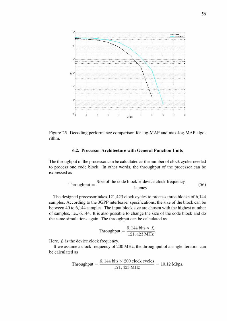
56

Figure 25. Decoding performance comparison for log-MAP and max-log-MAP algo-rithm.

6.2. Processor Architecture with General Function Units

The throughput of the processor can be calculated as the number of clock cycles neededto process one code block. In other words, the throughput of the processor can beexpressed as

Throughput =Size of the code block× device clock frequency

latency. (56)

The designed processor takes 121,423 clock cycles to process three blocks of 6,144samples. According to the 3GPP interleaver specifications, the size of the block can bebetween 40 to 6,144 samples. The input block size are chosen with the highest numberof samples, i.e., 6,144. It is also possible to change the size of the code block and dothe same simulations again. The throughput can be calculated as

Throughput =6, 144 bits× fc121, 423 MHz

.

Here, fc is the device clock frequency.If we assume a clock frequency of 200 MHz, the throughput of a single iteration can

be calculated as

Throughput =6, 144 bits× 200 clock cycles

121, 423 MHz= 10.12 Mbps.

57

The 200 MHz clock frequency is easily achievable and that is why it is a very rea-sonable estimate. The clock cycle needed for a single trellis stage of the max-log-MAPcan be calculated as

CycleStage =121, 423/2

6, 144

= 9.88 cycles.

The number of operations for the processor architecture are listed in Table 4.

Table 4. Number of operationsOperation # of OPS

LDW 147,459STW 116,763ADD 945,628SUB 12,290MUL 45,234MAX 368,656SHL 30,108

STREAM 18,534

The number of addition operations does not only represent the addition for the al-gorithm, but for several other purposes like loop indexing. The subtraction operationsare due to the normalization method used for the design. The multiplication is used forthe QPP interleaving sequence generation.

The utilization of buses is satisfactory for this processor. However, there is a lot ofspace to improve bus utilization for this design. Table 5 lists the usage of the buses inthis processor.

6.3. Processor Architecture with Special Function Unit

The performance of the architecture with special function units is described in thissection. The throughput calculation is done following (56).

The designed processor takes 39,226 clock cycles to process three blocks of 6,144samples for a full iteration for the max-log-MAP. The size of the input blocks is chosenas 6,144.

When we assume a clock of 200 MHz, the throughput of a single iteration for themax-log-MAP can be calculated as

Throughput =6, 144 bits× 200 clock cycles

39, 226 MHz= 31.32 Mbps.

The clock cycle needed for a single trellis stage of the max-log-MAP can be calcu-lated as

CycleStage =39, 226

2× 6, 144

= 3.19 cycles.

58

Table 5. Usage of busesIndex of the Buses Usage Index of the Buses Usage

1 15.76% 16 30.37%2 85.64% 17 34.50%3 88.64% 18 32.30%4 21.15% 19 35.27%5 59.42% 20 39.27%6 64.74% 21 41.24%7 56.07% 22 41.08%8 57.78% 23 44.49%9 66.03% 24 46.40%

10 68.97% 25 46.33%11 72.39% 26 48.46%12 79.87% 27 52.10%13 21.54% 28 52.91%14 24.70% 29 52.88%15 27.92% 30 51.59%

Table 6. Number of clock cycles for a full iterationMode Algorithm Clock Cycle

1 max-log-MAP 39,2262 linear-log-MAP 103,4363 constant-log-MAP 184,4544 log-MAP 834,253

It can be seen from Table 6 that the processor takes more clock cycles if max-log-MAP algorithm is not used. The reason lies in the fact that the constant-log-MAP,linear-log-MAP and log-MAP algorithms need to invoke some conditional statementresulting in branches in execution, and thus, increase latency compared to the max-log-MAP algorithm. A less complicated approximation of log-MAP is used in this design.However, the correction term of the log-MAP increases the latency significantly com-pared with the other three suboptimal algorithms even after the simplification. Linear-log-MAP is slower than the constant-log-MAP because of some multiplication opera-tions are needed. The log-MAP algorithm provides the best BER performance than theother algorithms. This log-MAP can be used in cases when the latency requirementsare not strict and a high BER performance is needed.

The number of some of the operations during the algorithm execution is summa-rized in Table 7. The reason for the high number of addition operations is the samefor the processor with general function units. The reason behind the subtraction andmultiplication operations is also the same.

The buses of the processor are optimally utilized to achieve the best possible resultdue to good scheduling. The usage of buses is given in Table 8.

The throughput can be increased using dedicated special function units working asaccelerators for the processor. On the other hand, the more special function unit isused, the less flexible the processor becomes. As an example, a special function unit

59

Table 7. Number of operationsOperation # of OPS

ADD 339,009SUB 98,304MUL 45,234

MAX7 24,567BRANCH 24,576STREAM 24,556

Table 8. Usage of busesIndex of the Buses Usage Index of the Buses Usage

1 97.32% 16 77.01%2 98.62% 17 88.09%3 98.63% 18 95.99%4 99.28% 19 95.99%5 99.28% 20 95.99%6 99.29% 21 95.99%7 99.67% 22 96.65%8 99.96% 23 96.65%9 94.69% 24 96.66%

10 92.45% 25 96.66%11 93.37% 26 79.26%12 89.28% 27 80.18%13 89.79% 28 81.38%14 91.25% 29 83.75%15 91.91% 30 85.46%

dedicated to calculate the backward metric and the LLRs could be designed to reducelatency. However, this special function unit might be useless for some other function-alities. A common special function unit to calculate both forward and backward metriccould be better utilized in this case.

The TTA processor designed here will work for the Viterbi decoding with reasonablethroughput. The BRANCH unit is able to calculate the add-select-compare operationsneeded for the Viterbi decoding.

6.4. Comparison

A comparison with different other programmable implementations of turbo decoder ispresented in Table 9. Our proposed processor provides very good throughput comparedto most of the programmable implementations. The decoder proposed in [28] wasimplemented on Pentium and the Windows 2000 operating system. As the decoderwas implemented in a general purpose processor, the throughput is low.

The turbo decoder presented in [44] was implemented on Motorola’s DSP56603.The performance was 50% higher than with ST120 with VLIW architecture. The

60

Table 9. Programmable processorsReference Architecture Algorithm Throughput

[44] Motorola max-log-MAP 243 Kbps[28] Intel Pentium max-log-MAP 366 Kbps[45] TMS320C6201 DSP max-log-MAP 2 Mbps[46] VLIW ASIP max-log-MAP 5 Mbps[5] TTA proc. for UMTS max-log-MAP 14.1 Mbps

This thesis TTA proc. max-log-MAP 31.21 Mbps[5] TTA proc. max-log-MAP 98 Mbps

throughput was still low compared to the other programmable implementations. Theturbo decoder presented in [45] was implemented on TMS320C6201 DSP developedby TI. An optimized C code was written for the processor. However, the performancewas still not satisfactory. The implementations of [28], [44] and [45] used readilyavailable processors in the market. The throughputs were low because no dedicatedhardware was designed for the particular software implementations.

A turbo decoder application-specific instruction-set (ASIP) was designed in [46] andwas prototyped in a Xilinx Virtex 4000 FPGA. The decoder was better than the ear-lier programmable implementations, but the throughput was still not satisfactory forthe 3GPP LTE sytems. One of the best implementations for a programmable turbodecoder was done in [5]. The throughput of the design was comparable with purehardware designs. However, the biggest drawback of the design is the inflexibility ofthe processor. The processor used dedicated special function units for forward metric,backward metric and branch metric calculations. These units were designed only forthe max-log-MAP algorithm. Therefore, it would be difficult to program the processorfor the other algorithms, as the main calculations are done in the special function units.The author did not show how the special function units could be used for log-MAP,constant-log-MAP and linear-log-MAP algorithms. Besides, the turbo code designedfor the processor was not according to 3GPP LTE or UMTS specifications. The pro-cessor implemented in this thesis has lower throughput than the TTA processor of [5]for the same clock frequency of 200 MHz. The use of the complex QPP interleavingis the reason behind it.

61

7. DISCUSSION

The processor with the general function unit is designed for the max-log-MAP algo-rithm. As already stated, this processor is very flexible but its relative less throughputmakes it unsuitable for using with the latest standards like LTE with high data rates.

The second processor with the special function unit provides higher data rate formax-log-MAP algorithm. However, the throughput could be increased more. The im-plementations for the other algorithms need to be more carefully investigated. TheQPP interleaving and de-interleaving is a significant bottleneck in a single core pro-cessor. Its contention free interleaving and de-interleaving properties cannot be fullyutilized for a single core processor. In the multi-core processor, the benefits of QPPinterleaving and de-interleaving pattern could be fully utilized.

The word length studies are not done on a link level simulator. However, a wordlength of 8-bits can be used. Thus, 4 inputs can be transferred through the buses by a32-bit word [5]. The word length studies can be done in the future for the exact wordlength requirements.

The processors are not synthesized. Therefore, the number of gate counts is notproperly calculated. The processors need to be mapped on the FPGA and many unnec-essary units need to be eliminated during the design process, if the processor becomestoo complex.

The theoretical peak data rate for LTE is 326.4 Mbps. It is difficult to reach thedata rate of 100 Mbps, which is the first milestone to reach the peak, even with ahardware implementation for the turbo decoder. The only solution is to use the parallelarchitecture method to reach 100 Mbps and beyond [47].

There are three parallelism methods for enhancing decoder speed. The turbo decoderlevel parallelism, the SISO decoder level parallelism and the trellis stage level. Thetrellis stage parallelism reduces the latency by processing more trellises between twotime instances. However, this parallelism is not enough to increase the data rate close tothe LTE requirement. Several turbo decoders working in parallel as co-processors aredefined as turbo decoder level parallelism. The most promising solution for a parallelarchitecture is to use several SISO decoding processors in parallel as co-processors.This parallelism method is called the SISO decoder level parallelism [48]. A blockdiagram of such a parallel turbo decoder processor is presented in Figure 26. Another

Figure 26. Parallel turbo decoder.

62

aspect to consider for a parallel turbo decoder is the type of the processors used forthe design. The design could either be homogeneous, heterogeneous or a hybrid. In ahomogeneous multi-processor system, all the processors perform the same task. In aheterogeneous system, the application is divided in different parts and each processordoes different tasks. The homogeneous system is better for parallel turbo decoderbecause there is a lot of data dependencies. Therefore, the heterogeneous processorwill not be able to process each parts independently in parallel. A homogeneous systemof same SISO decoding processors will be ideal in this case.

In this thesis work, the highest throughput is achieved through the processor withspecial function unit working on the max-log-MAP mode. The throughput of thisprocessor is 31.21 Mbps. Therefore, six to eight of these processors running in parallelcould reach more than 100 Mbps of throughput if they are scheduled correctly.

The parallel turbo decoder’s performance will depend on how good the individualcores are and how good the scheduling is. The throughput of the parallel turbo de-coder will depend on the processors like the ones designed in this thesis. The futureembedded systems for LTE need to have multi-core setups to provide the high datarates.

63

8. SUMMARY

The purpose of this thesis was to implement an iterative turbo decoder as an ASSP. TheASIC implementations of turbo decoder provides good throughput, but are not flexibleto provide support for different standards. The GPP or the DSP implementations ofturbo decoder suffers from lower throughput. Therefore, the turbo decoder was imple-mented as an ASSP. TTA processor architecture was chosen for the ASSP to providesufficient throughput and flexibility.

Turbo decoder was first simulated in a MATLAB link level simulator. The simulatedturbo decoder design was too complex to implement for the hardware. Therefore,several techniques to simplify the MAP algorithm were used. An approximation ofthe log-MAP algorithm was used as it was more complex than other subgradient MAPalgorithms.

The QPP interleaver was used in the design to make the processor 3GPP LTE com-pliant. The complex interleaving and de-interleaving was one of the bottlenecks toimplement the turbo decoder in hardware.

The MATLAB design was then converted and optimized in C language and mappedon the TTA processor using TCE tool. Two processors were designed for the turbo de-coder application. The first processor was built using the basic function units and wasdesigned to support the max-log-MAP algorithm. The second processor was designedwith special function units and was able to support max-log-MAP, log-MAP, constant-log-MAP and linear-log-MAP algorithm. Two special function units were built for thisprocessor. One special function unit was used to calculate the forward and backwardmetrics and the other special function unit was used to calculate the LLR values.

The processor with general function units was more flexible, but provides lowerthroughput. The second processor was flexible and provides good throughput also. Thesecond processor showed the promise of the possibility of designing several decodingtechniques on a single TTA processor.

The researchers are focusing on the parallel turbo decoder implementation, whereseveral SISO decoder ASIC or processors work parallely to provide LTE targetthroughput. As the turbo decoding algorithm is very complex, it is very difficult toachieve the LTE target throughput even with pure hardware designs. The parallelmulti-core turbo decoder is the natural choice for the next generation wireless sys-tems. The target throughput could also be reached by TTA processor by implementingon multi-core. The flexibility gained from that processor could provide very interestingresults and would be a fruitful direction for future research.

64

9. REFERENCES

[1] Shannon C.E. (1948) A mathematical theory of communication. Bell SystemTechnical Journal 27, pp. 379–423 and 623–656.

[2] Berrou C., Glavieux A. & Thitimajshima P. (1993) Near shannon limit error-correcting coding and decoding: turbo-codes. In: IEEE International Conferenceon Communication, vol. 2, Geneva, Switzerland, vol. 2, pp. 1064–1070.

[3] Evolved universal terrestrial radio access (E-UTRA); Multiplexing and channelcoding, 3GPP TS version 36.212.

[4] Jääskeläinen P., Guzma V., Cilio A. & Takala J. (2007) Codesign toolset forapplication-specific instruction-set processors. In: Proc. SPIE Multimedia onMobile Devices, pp. 65070X–1 – 65070X–11.

[5] Salmela P., Sorokin H. & Takala J. (2008) A programmable max-log-MAP turbodecoder implementation. Hindawi VLSI Design 2008, pp. 636–640.

[6] Goldsmith A. (2005) Wireless Communications. Cambridge University Press,New York, USA.

[7] Hochwald B.M. (2003) Achieving near-capacity on a multiple-antenna channel.IEEE Transactions on Communications 51, pp. 389–399.

[8] Tarokh V., Jafarkhani H. & Calderbank A.R. (1999) Space-time block codes fromorthogonal designs. IEEE Transactions on Information Theory 45, pp. 1456–1467.

[9] Golden G.D., Foschini C.J., Valenzuela R.A. & Wolniansky P.W. (1999) Detec-tion algorithm and initial laboratory results using V-BLAST space-time commu-nication architecture. Electronics Letters 35, pp. 14–16.

[10] Ha J., Mody A.N., Sung J.H., Barry J.R., McLaughlin S.W. & Stüber G.L. (2002)LDPC coded OFDM with Alamouti/SVD diversity technique. Wireless PersonalCommunications 23, pp. 183–194.

[11] Yang H. (2005) A road to future broadband wireless access: MIMO-OFDM-Based air interface. IEEE Communications Magazine 43, pp. 53–60.

[12] Myllylä M. (2011) Detection algorithms and architectures for wireless spatialmultiplexing in MIMO-OFDM systems. Ph.D. thesis, University of Oulu, De-partment of Electrical and Information Engineering.

[13] Janhunen J. (2007) Signal processor implementation of list sphere detectors.Master’s thesis, University of Oulu.

[14] Ketonen J., Juntti M. & Cavallero J.R. (2010) Performance-complexity compar-ison of receivers for a LTE MIMO-OFDM system. IEEE Transactions on SignalProcessing 58, pp. 8–17.

65

[15] MacKay D. (2003) Information theory, inference, and learning algorithms. Cam-bridge University Press, Cambridge, UK.

[16] Viterbi A.J. (1967) Error bounds for convolutional codes and an asymptoticalllyoptimal decoding algorithm. IEEE Transactions on Information Theory IT-13,pp. 260–269.

[17] Massey J.L. (1965) Step-by-step decoding of the Bose-Chaudhuri-Hocquenghemcodes. IEEE Transactions on Information Theory 11, pp. 580–585.

[18] Wicker S.B. & Bhargava V.K. (1994) Reed-Solomon codes and their applications.IEEE press, New York.

[19] Alamouti S.M., Tarokh V. & Poon P. (1998) Trellis-coded modulation and trans-mit diversity: design criteria and performance evaluation. In: IEEE ICUPC 98,pp. 702 – 707.

[20] Guizzo E. (2004) Closing in on the perfect code. IEEE Spectrum Magazine 41,pp. 36–42.

[21] Elias P. (1955) Coding for noisy channels. IRE Conv. Rec. 4, pp. 37–46.

[22] Sklar B. (1997) A primer on turbo code concepts. IEEE Communications Maga-zine 35, pp. 94–102.

[23] Bahl L.R., Cocke J., Jelinek F. & Raviv J. (1974) Optimal decoding of linearcodes for minimizing symbol error rate. IEEE Transactions on Information The-ory 20, pp. 284–287.

[24] Benedetto S., Montorsi G., Divsalar D. & Pollara F. (1996) A soft-input soft-output Maximum A Posteriori (MAP) module to decoder parallel and serial con-catenated codes. JPL TDA Progr. Rep. 1-20, pp. 2208–2233.

[25] Robertson P., Hoeher P. & Villebrun E. (1997) Optimal and suboptimal maximuma posteriori algorithms suitable for turbo decoding. European Trans. on Telecom-mun. 8, pp. 119–125.

[26] Classon B., Blankenship K. & Desai V. (2000) Turbo decoding with the constant-log-map algorithm. In: Proc., Second int. Symp. Turbo Codes and Related Appl.,Brest, France, pp. 467–470.

[27] Cheng J. & Ottosson T. (2000) Linearly approximated log-map algorithms forturbo coding. In: Proc., IEEE Veh. Tech. Conf., Houtson, TX.

[28] Valenti M.C. & Sun J. (2001) The UMTS turbo code and an efficient decoder im-plementation suitable for software defined radiosr. International Journal on Wire-less Information Networks 8, pp. 203–216.

[29] Ryu J.H. (2007) Permutation polynomial based interleavers for turbo codes overinteger rings: theory and applications. Ph.D. thesis, The Ohio State University.

66

[30] Takeshita O.Y. (2006) On maximum contention-free interleavers and permutationpolynomials over integer rings. IEEE Transactions on Information Theory 52, pp.1249–1253.

[31] Sun Y. & Cavallaro J.R. (2010) Efficient hardware implementation of a highly-parallel 3GPP LTE, LTE-advance turbo decoder. Integr.,VLSI J. 44, pp. 1–11.

[32] (accessed 28.8.2012.), ARM. URL: http://www.arm.com/.

[33] (accessed 28.8.2012.), MIPS. URL: http://www.mips.com/.

[34] (accessed 28.8.2012.), Texas Instruments. URL: http://www.ti.com/.

[35] Patterson D.A. (1980) The case for reduced instruction set computer. ACMSIGARACH Computer Architecture News 8, pp. 25–33.

[36] Hu S., Kim I., Lipasti M.H. & Smith J.E. (2006) An approach for implementingefficient superscalar cisc processors. In: The Twelfth International Symposiumon High-Performance Computer Architecture, pp. 41 – 52.

[37] Fisher J.A., Faraboschi P. & Young C. (2004) A VLIW approach to architecture,compilers and tools. Morgan Kaufmann.

[38] Corporaal H. (1997) Microprocessor Architectures: From VLIW to TTA .

[39] Pitkänen T. (2005) Experiments of TTA on ASIC technology. Master’s thesis,Department of Electrical Engineering, Tampere University of Technology.

[40] Tabak D. & Lipovski G.J. (1980) MOVE Architecture in Digital Controllers.IEEE Journal of Solid-State Circuits 15, pp. 116 – 126.

[41] Jääskeläinen P. (2005) Instruction set simulator for transport triggered architec-tures. Master’s thesis, Department of Information Technology, Tampere Univer-sity of Technology.

[42] Esko O. (2011) ASIP integration and verification flow for FPGA. Master’s thesis,Tampere University of Technology.

[43] Salmela P., Järvinen T. & Takala J. (2007) Simplified max-log-map decoder struc-ture. In: Proceedings of the 1st Joint Workshop on Mobile Future and the Sym-posium on Trends in Communications (SympoTIC ’06), San Jose, Calif, USA,pp. 1–11.

[44] Michel H., Worm A., Munch M. & Wehn N. (2002) Hardware software trade-offsfor advanced 3g channel coding. In: Proceedings of Design, Automation and Testin Europe.

[45] Song Y., Liu G. & Huiyang (2005) The implementation of turbo decoder on dspin w-cdma system. In: International Conference on Wireless Communications,Networking and Mobile Computing, pp. 1281–1283.

67

[46] Ituero P. & Lopez-Vallejo M. (2006) New schemes in clustered vliw proces-sors applied to turbo decoding. In: Proceedings of International Conference onApplication-Specific Systems, Architectures and Processors (ASAP ’06), Steam-boat Springs, Colo, USA, pp. 291–296.

[47] Studer C., Benkeser C., Belfanti S. & Huang Q. (2011) Design and implementa-tion of a parallel turbo-decoder ASIC for 3GPP LTE. IEEE Journal on Solid-StateCircuits 46, pp. 8–17.

[48] Wong C.C., Lai M.W., Lin C.C., Chang H.C. & Lee C.Y. (2010) Turbo decoderusing contention-free interleaver and parallel architecture. IEEE Journal on Solid-State Circuits 45, pp. 422–432.