design of an engine hoist - umich.edudesci501/2003/apd-2003-09.pdf · design of an engine hoist by...
TRANSCRIPT

DESIGN OF AN ENGINE HOIST
by
Lara Sherefkin Alice Jakobsen
ME 09-599 Fall 2003
Final Report
The following work has been done in an effort to find the optimal design of an engine hoist. Using an engineering model, the initial optimization was done with the goal of minimizing the overall weight of the hoist. Subsequently, a microeconomic model was created to re-optimize the design problem, maximizing profit in production. To further validate the economic model, a survey was given and conjoint analysis used to determine attribute elasticities. The attributes that were considered were those deemed to be the most important to potential consumers. These include the maximum feasible load capacity, the maximum height that the hoist can lift, and the price. Finally, three product families were established. The objective of each of the models was weighted and combined to give an overall score. This combined score was then maximized over different sets of weights using two separate sets of commonality constraints. In conclusion, for the economic model, the outcome of the survey showed that to consumers load capacity and price were the most important of the attributes. It was then found that the maximum profit that could be obtained, taking into consideration the costs associated with production, was $4,278,967 for a hoist that could lift just over two tons to a height of 7.79 feet and would cost $277.
Table of Contents Table of Contents................................................................................................................ 2 Nomenclature...................................................................................................................... 3 1. Introduction................................................................................................................. 5
1.1. The product design problem ............................................................................... 5 1.2. Product development process ............................................................................. 5 1.3. Design Requirements .......................................................................................... 6 1.4. Product decisions from the design phase ............................................................ 7 1.5. Design requirements that can be quantified........................................................ 7 1.6. Design requirements that can be quantified using engineering analysis ............ 7
2. Engineering Design Model ......................................................................................... 8 2.1. Design optimization problem.............................................................................. 8 2.2. Analysis model.................................................................................................... 9 2.3. Optimization model in negative null form........................................................ 11 2.4. Optimization results .......................................................................................... 11
3. Model Extension: Microeconomics .......................................................................... 12 3.1. Competitors....................................................................................................... 12 3.2. Maximization of profit ...................................................................................... 15 3.3. Results............................................................................................................... 19
4. Model Extension: Marketing .................................................................................... 19 4.1. Market size........................................................................................................ 19 4.2. Determining betas ............................................................................................. 20 4.3. Linearized demand function, Qm ...................................................................... 22 4.4. Comparison of elasticities and intercept ........................................................... 23 4.5. Re-optimization of design decision model ....................................................... 23 4.6. Comparison of results ....................................................................................... 24
5. Product Family Design ............................................................................................. 25 5.1. Market segments ............................................................................................... 25 5.2. Design optimization models ............................................................................. 25 5.3. Separate design optimizations........................................................................... 26
a. Load capacity .................................................................................................... 26 b. Lifting height .................................................................................................... 27 c. Price (operating variable cost) .......................................................................... 28
5.4. Creating Pareto surface with first set of commonality constraints ................... 29 5.5. Pareto surface with second set of commonality constraints ............................. 31
6. Conclusions............................................................................................................... 33 7. Appendices................................................................................................................ 34
5.1. Appendix A: Patent images .............................................................................. 34 7.2. Appendix B: Initial fixed investment and variable cost.................................... 37
Business plan .................................................................................................................... 40 A) Business opportunity............................................................................................. 40
a) Business objective................................................................................................. 40 b) Product description ............................................................................................... 40 c) Market analysis ..................................................................................................... 41
B) Financial data ........................................................................................................ 42

a) Capital equipment and supply list......................................................................... 42 b) Breakeven analysis................................................................................................ 43 c) Pro-forma income and cost projections ................................................................ 44
I) Annual cost ....................................................................................................... 44 II) Net profit after depreciation and taxes.......................................................... 44
C) Supporting documents .......................................................................................... 45 a) Existing patents..................................................................................................... 45 b) Technical analysis and benchmarking .................................................................. 47
8. Slut ............................................................................................................................ 48
Nomenclature
A Total length of boom a Cross section area of tubing C Cost C0 Initial fixed investment C1 Operating variable cost per hoist d Diameter of hoist tubing (square) F1 Force on boom from the load at edge of boom F2 Force on boom where jack is attached F3 Force on boom where attached to back F4 Vertical force on back where attached to bottom G Gravity t Thickness of hoist tubing I Moment of inertia of tubing h1 Height of boom when jack fully compressed h2 Height of boom when in horizontal position h3 Height of boom when jack fully extended h3 Height of boom when jack fully extended l1 Distance from front edge, on boom, to where jack is mounted l2 Distance from hoist body, on boom, to where jack is mounted l5 Horizontal distance from back top to back were jack is attached l6 Distance along hoist back between top and point of jack attachment l9 Horizontal distance from back top to back bottom lj,e Length of the jack fully extended lj,c Length of the jack fully compressed M2 Moment on back where attached to bottom Mmaxback Maximum moment in back Mmaxboom Maximum moment in boom
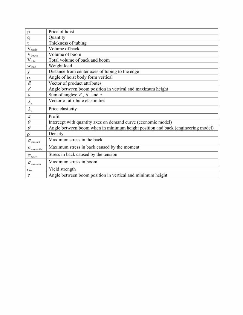
p Price of hoist q Quantity t Thickness of tubing Vback Volume of back Vboom Volume of boom Vtotal Total volume of back and boom wload Weight load y Distance from center axes of tubing to the edge α Angle of hoist body form vertical αr Vector of product attributes δ Angle between boom position in vertical and maximum height ε Sum of angles: δ , θ , and τ
aλr
Vector of attribute elasticities
pλ Price elasticity π Profit θ Intercept with quantity axes on demand curve (economic model) θ Angle between boom when in minimum height position and back (engineering model) ρ Density
max backσ Maximum stress in the back
max backMσ Maximum stress in back caused by the moment
backTσ Stress in back caused by the tension
max boomσ Maximum stress in boom σy Yield strength τ Angle between boom position in vertical and minimum height

1. Introduction Figure 1 below shows an example of a standard engine hoist.
Figure 1: Engine hoist
1.1. The product design problem The intended user of this product is both commercial garages and private at-home mechanics. For these users, the engine hoist should have the following characteristics. These include choosing dimensions that minimize weight so the hoist is easy to move around, but which also maintain the required functionality in weight capacity. En addition the design must have an acceptable range of operating angles to accommodate the change in vertical height required by the user. The product should also fold up into a more compact form and should be easy to operate. Also important is the need for the product to be inexpensive and for the load capacity to be able to be changed by adjusting the length of the boom.
1.2. Product development process The product development process of an engine hoist is illustrated below.
Initialization There is market demand for something that can lift engines easily out of car.
The company wants to begin producing a product that fills the market demand.
Marketing analysis What is the goal of the company in the market?
The market segment will be commercial garages and the at-home mechanic. The goal is to reach these segments by producing a product that will satisfy the design requirements.

1.3. Design Requirements
Product definition The market is for a product that can easily lift heavy loads and fit into tight spaces.
Product must be able to support required loads, not exceed a specified size, and be of minimum weight.
Idea generation
The product should fold up for space savings in storage, and it should be possible to adjust the length of the boom (and thereby load capacity). The product should also be able to be easily moved around. The operating height should have a sufficiently large range of motion using an existing hydraulic ram.
General product goals have been established and existing technology examined.
Concept evaluation The desired product characteristics have been determined.
Criteria such as material availability and cost have been applied to the generated ideas.
Design optimization Concepts that fulfill all basic requirements. Functional design constraints.
Final design.
Prototype Design specifications.
Does the model work? A model for evaluation, for testing, and for consumer focus groups.
Testing How robust is the product? Life cycle durability. Determine warranty issues.
Physical model
Sales
Marketing strategy
Results from consumer focus groups.
Plan for a marketing campaign.
Production planning
How the product will be mass-produced, what facilities will be used, who the suppliers will be, and how the product will be distributed.
Changes are made to design.
Production Final productFinal design specifications

The product must be able to lift a specified range of loads. The boom must be long enough to reach and support the load (clearance issues). Using an existing hydraulic ram, the product must be able to move through a
specified range of operating heights. The total weight should be minimal such that it can easily be moved around. The appearance of the product must be appealing. The cost of the produce must be minimal. The product should be able to fold up into a smaller volume for ease of storage
and transportation. The load capacity of the hoist should be able to be changed by adjusting the
length of the boom.
1.4. Product decisions from the design phase The design phase, which encompasses product definition through design optimization, the product decisions that can be made include: Topology Load capacity Appearance Size (in use) Ability to move around Durability Manufacturing considerations
1.5. Design requirements that can be quantified
The design must be able to lift a specified range of loads. The boom must be long enough to reach and support the load. The hoist must be tall enough to reach into standard size cars and trucks. The product must be able to move through a specified range of operating heights. The product should be light enough to easily move around. The product must have minimal cost. The hoist must be durable. The design must be able to be produced easily and with as few parts as possible.
1.6. Design requirements that can be quantified using engineering analysis
The design must be able to lift a specified range of loads. The boom must be long enough to reach and support the load. The hoist must be tall enough to reach into standard size cars and trucks.

The product must be able to move through a specified range of operating heights. The product must have minimal cost. The hoist must be durable. The product must have minimal weight.
2. Engineering Design Model
2.1. Design optimization problem
Assumptions: In this model the hoist will be represented as the hoist body and attached boom, the legs not being considered. The material for the hoist body and boom will be AISI 1018 steel square tubing and both will have the same cross sectional area. Cost will not be considered. For the jack used in the design it is assumed that it is sufficiently strong enough to support all loads without buckling, deforming, or otherwise affecting the performance of the hoist (including a factor of safety). Objective: Minimize weight. Parameters: Hydraulic ram operating capacities; density an strength of material; load capacity. Variables: Height of boom when jack is perpendicular to ground; length of jack’s extension at boom horizontal position; distance from hoist body where the jack is mounted to the boom; angle of hoist body form vertical; thickness of boom and hoist back; width of outer boom and hoist back. Constraints: Height of boom when jack fully compressed must be less than the height of the boom in horizontal position which must also be less than the height of the boom at jack full extension. The length of the jack fully compressed must be less than when the jack is at boom horizontal position which must also be less than when the jack is fully extended. The mounting point at the jack on the boom can be no longer than the length of the boom itself. The maximum stress that the boom I seeing form the load must be no more than the yield strength of the material. The angle of the hoist back can be between 0 to 90 degrees. The location of the jack on the hoist body must be at or above the total length of the hoist. The thickness of the material must be at least 1mm and the outer diameter must be between 2mm and 15cm. Finally, the angles that the boom makes at the various positions must each be less than 90 degrees.

2.2. Analysis model
The variables, parameters, and functions used to calculate the objective equation and constraints are given below: Variables: h2 = height of boom from ground when in horizontal position α = angle of hoist body form vertical l2 = distance form hoist body, on boom, where jack is mounted l6 = distance along hoist back between top and point of jack attachment t = thickness of hoist tubing d = diameter of hoist tubing (square)
Parameters: ρ = density wload = weight load g = gravity A = total length of boom σy = yield strength lj,e = length of the jack fully extended lj,c = length of the jack fully compressed h1 = height of boom when jack fully compressed h3 = height of boom when jack fully extended
Figure 2: Boom FBD and moment forces
F1F2F3
l2 l1
-F1*l1
M
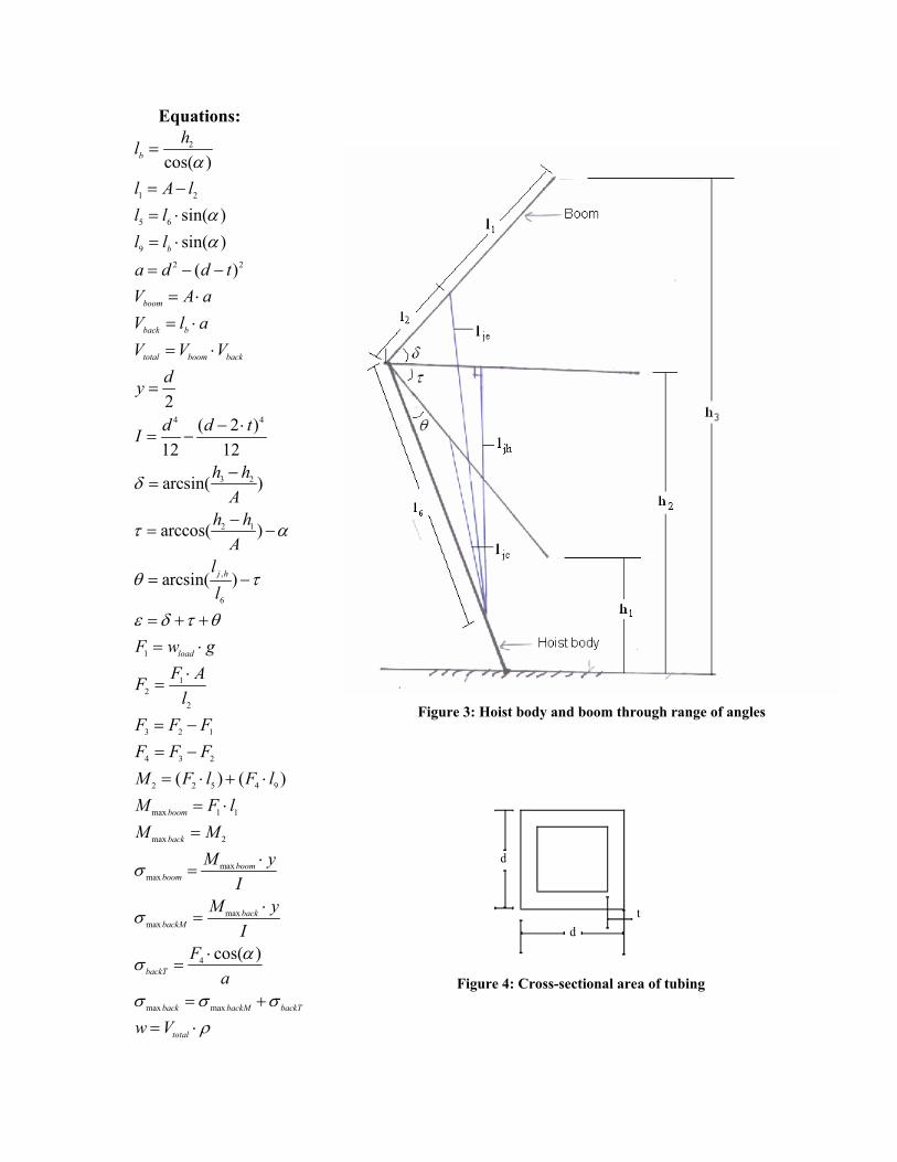
Equations:
Figure 3: Hoist body and boom through range of angles
2
1 2
5 6
9
2 2
4 4
3 2
2 1
,
6
1
12
2
3 2 1
4
cos( )
sin( )sin( )
( )
2( 2 )
12 12
arcsin( )
arccos( )
arcsin( )
b
b
boom
back b
total boom back
j h
load
hl
l A ll ll la d d tV A aV l aV V V
dy
d d tI
h hA
h hA
ll
F w gF AF
lF F FF
α
αα
δ
τ α
θ τ
ε δ τ θ
=
= −= ⋅= ⋅
= − −= ⋅= ⋅= ⋅
=
− ⋅= −
−=
−= −
= −
= + += ⋅
⋅=
= −= 3 2
2 2 5 4 9
max 1 1
max 2
maxmax
maxmax
4
max max
( ) ( )
cos( )
boom
back
boomboom
backbackM
backT
back backM backT
total
F FM F l F lM F lM M
M yI
M yI
Fa
w V
σ
σ
ασ
σ σ σρ
−= ⋅ + ⋅
= ⋅=
⋅=
⋅=
⋅=
= += ⋅
dt
d
Figure 4: Cross-sectional area of tubing

2.3. Optimization model in negative null form
F3
F2
F4
l6
l7M2
Figure 5: Hoist body FBD
1 max
2 max
3
4
5 2
6 2
7
8 6
9 2
10
2 2 21 2 6 2 6 ,
2 22 2 6 2 6
minsubject to
00
0.0016 00.01 0
0.127 0
020.2 0
0.127 01.219 0
2 02 cos( ) 0
2 c
back y
boom y
b
j c
w
ggg tg dg l
Ag l
gg l lg hg d th l l l l l
h l l l l
σ σ
σ σ
α
τ
= −
= −
= − + ≤= − ≤= − + ≤
= − ≤
= − + ≤= − + ≤= − + ≤= − ⋅ ≤
= + − ⋅ ⋅ ⋅ − =
= + − ⋅ ⋅ ⋅
<
<
2,os( ) 0j elε − =
M
F3 F2
F4
M2M2
Figure 6: Hoist body moment diagram
2.4. Optimization results
Table 1 below shows that parameter values used in the model.
Parameters:density = 7870weight load = 1000g = 9.81jack extented, lje = 1.14jack compressed, ljc = 0.58minimum height, h1 = 0.025maximum height, h3 = 2.5yeild strength, sy = 3.70E+08total length of boom, A = 1.3
Table 1: Parameter values
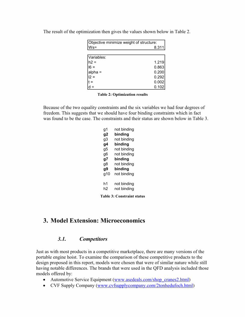
The result of the optimization then gives the values shown below in Table 2.
Objective minimize weight of structure:Ws= 8.311
Variables:h2 = 1.219l6 = 0.863alpha = 0.200l2 = 0.292t = 0.002d = 0.102
Table 2: Optimization results
Because of the two equality constraints and the six variables we had four degrees of freedom. This suggests that we should have four binding constraints which in fact was found to be the case. The constraints and their status are shown below in Table 3.
g1 not bindingg2 bindingg3 not bindingg4 bindingg5 not bindingg6 not bindingg7 bindingg8 not bindingg9 bindingg10 not binding
h1 not bindingh2 not binding
Table 3: Constraint status
3. Model Extension: Microeconomics
3.1. Competitors Just as with most products in a competitive marketplace, there are many versions of the portable engine hoist. To examine the comparison of these competitive products to the design proposed in this report, models were chosen that were of similar nature while still having notable differences. The brands that were used in the QFD analysis included those models offered by:
• Automotive Service Equipment (www.asedeals.com/shop_cranes2.html) • CVF Supply Company (www.cvfsupplycompany.com/2tonhedufoch.html)

• Cummins Industrial Tools (www.cumminstools.com/browse.cfm/4,193.html) • Jiangsu Tongrun Machinery & Electrical Appliance Imp & Exp Co., LTD
The completed QFD for the competitor analysis is shown below in Table 4. Here we see the technical analysis of the competition below the consumer requirements and the design analysis to the right of the design requirements. For ease of reproduction, a 0 to 3 scale has been used in place of the traditional symbols. The key is given in the bottom right hand corner of the table.
Table 4: QFD
Leng
th o
f boo
m
Thic
knes
s of
mat
eria
l
Leng
th o
f bac
k
Col
or
Dia
met
er
Mat
eria
l typ
e
Jack
cap
acity
Jack
pla
cem
ent
Size
ope
n
Size
clo
sed
Cas
ters
Wel
d ty
pe
Pins
ASE
CVF
CU
MM
INS
Jian
gusy
Our
Should lift 2 ton 2 3 1 0 3 3 3 0 0 0 3 3 3 1 3 3 3 3Boom lenght 3 2 1 0 2 2 0 0 3 3 0 0 0 2 3 3 3 3Range of boom height 3 0 1 0 0 0 3 3 3 0 0 0 0 2 3 2 2 3Minimal weight 2 3 2 0 3 3 1 0 2 2 1 0 0 3 2 2 2 3Apparance 0 0 0 3 0 0 0 0 1 2 1 1 1 1 3 3 3 3Cost 2 2 2 0 2 2 3 0 1 2 2 1 1 1 3 3 3Can fold up 1 0 1 0 0 0 0 2 0 3 1 0 1 3 3 3 3 3Minimal size when folded 2 0 2 0 1 1 0 2 0 3 0 0 0 3 2 2 2 2Height of hoist/back 0 1 3 0 1 1 0 0 3 3 0 0 0 3 3 3 3 3ASE 2 3 3 3 3 3 3 3 3 3 2 3 3 RelationshipsCVF 3 3 3 3 3 3 3 3 2 2 3 3 3 Strong 3CUMMINS 3 3 3 3 3 3 3 3 2 2 2 3 3 Medium 2Jiangsu 3 3 3 3 3 3 3 3 2 2 2 3 3 Weak 1Ours 3 3 3 3 3 3 3 3 2 2 3 3 3 None 0C
ompa
nies
QFD
Cus
tom
er re
quire
men
ts
Design requirements Companies
Following the QFD, the next step was a patent search. The abstract of the patent found is given below, with the patent information given in Figure 7.
“A portable engine hoist which folds into a compact storage position. The base of the hoist is equipped with two support wheels. Two elongated legs extend from the base and are adapted to receive leg extensions. The leg extensions are provided with wheels at one end and the other end can be inserted into a leg. An upright post extends from a base support and carries a pivotally mounted lifting beam at its top end. A mechanical or hydraulic jack operates to raise and lower the lifting beam to raise and lower an engine. Position adjustment and maintenance means for easy assembly of the leg extensions are provided. A cam slot locking means associated with the lifting beam provides stability under the load”.

Figure 7: Engine hoist patent
To be even clearer on the make-up of the product, additional images are given in Appendix A.
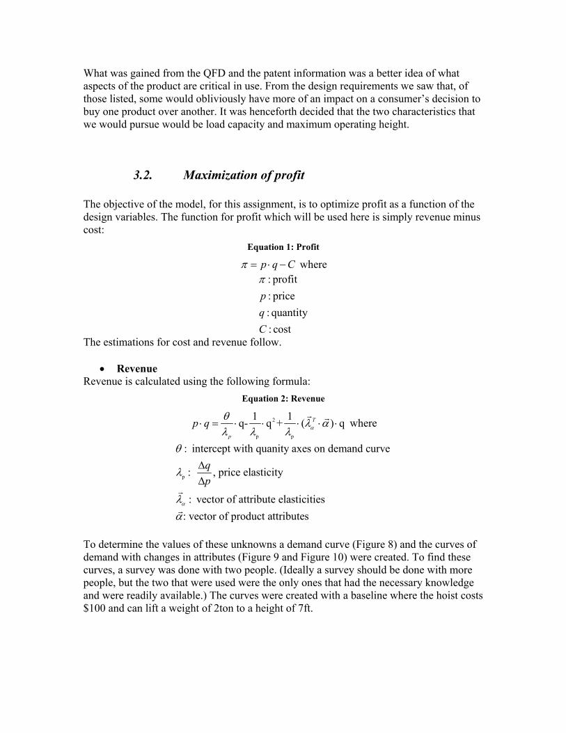
What was gained from the QFD and the patent information was a better idea of what aspects of the product are critical in use. From the design requirements we saw that, of those listed, some would obliviously have more of an impact on a consumer’s decision to buy one product over another. It was henceforth decided that the two characteristics that we would pursue would be load capacity and maximum operating height.
3.2. Maximization of profit The objective of the model, for this assignment, is to optimize profit as a function of the design variables. The function for profit which will be used here is simply revenue minus cost:
Equation 1: Profit
p q Cπ = ⋅ − where : profit: price: quantity: cost
pqC
π
The estimations for cost and revenue follow.
• Revenue Revenue is calculated using the following formula:
Equation 2: Revenue
2
p p
1 1q- q + ( ) qT
p
p q α
θ λ αλ λ λ
⋅ = ⋅ ⋅ ⋅ ⋅ ⋅r r where
p
: intercept with quanity axes on demand curve
: , price elasticity
: vector of attribute elasticities: vector of product attributes
qp
α
θ
λ
λα
∆∆
r
r
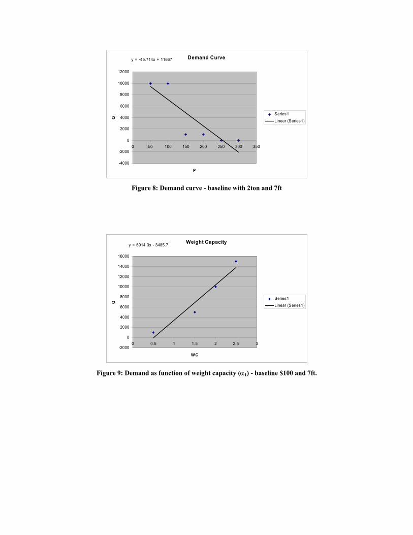
To determine the values of these unknowns a demand curve (Figure 8) and the curves of demand with changes in attributes (Figure 9 and Figure 10) were created. To find these curves, a survey was done with two people. (Ideally a survey should be done with more people, but the two that were used were the only ones that had the necessary knowledge and were readily available.) The curves were created with a baseline where the hoist costs $100 and can lift a weight of 2ton to a height of 7ft.
Demand Curvey = -45.714x + 11667
-4000
-2000
0
2000
4000
6000
8000
10000
12000
0 50 100 150 200 250 300 350
P
QSeries1Linear (Series1)
Figure 8: Demand curve - baseline with 2ton and 7ft
Weight Capacityy = 6914.3x - 3485.7
-2000
0
2000
4000
6000
8000
10000
12000
14000
16000
0 0.5 1 1.5 2 2.5 3
WC
Q
Series1Linear (Series1)
Figure 9: Demand as function of weight capacity (α1) - baseline $100 and 7ft.

Lifting Heighty = 3228.6x - 13819
-2000
0
2000
4000
6000
8000
10000
12000
14000
16000
18000
0 2 4 6 8 10
LH
QSeries1Linear (Series1)
Figure 10: Demand as function of lifting height (α2) - baseline $100 and 2ton.
From Figure 7 it is possible to determine the following:
11,700 and 46pθ λ= = − From Figure 8and Figure 9 respectively:
1 26,910 and 3,230α αλ λ= =
Finally, Equation 2 can be rewritten:
• Cost The cost for producing q engine hoists is giving by the following equation.
Equation 3: Cost
0 1C C C q= + ⋅ where
0
1
: initial fixed investment: operating variable cost per hoist
CC
The estimated values of C0 and C1 are summarized below in Table 5 and Table 6 respectively. Further explanation about the estimations can be found in Appendix B.
Table 5: Initial fixed investments, C0
Description Cost per year ($) Warehouse 12,000Utilities 1,200Salary 75,000
[ ] 12
2
11,700 1 1 ( 6,910 3,230 )46 46 46
p q q q qαα
∆ ⋅ = ⋅ − + ⋅ ⋅ ⋅ ∆− − −
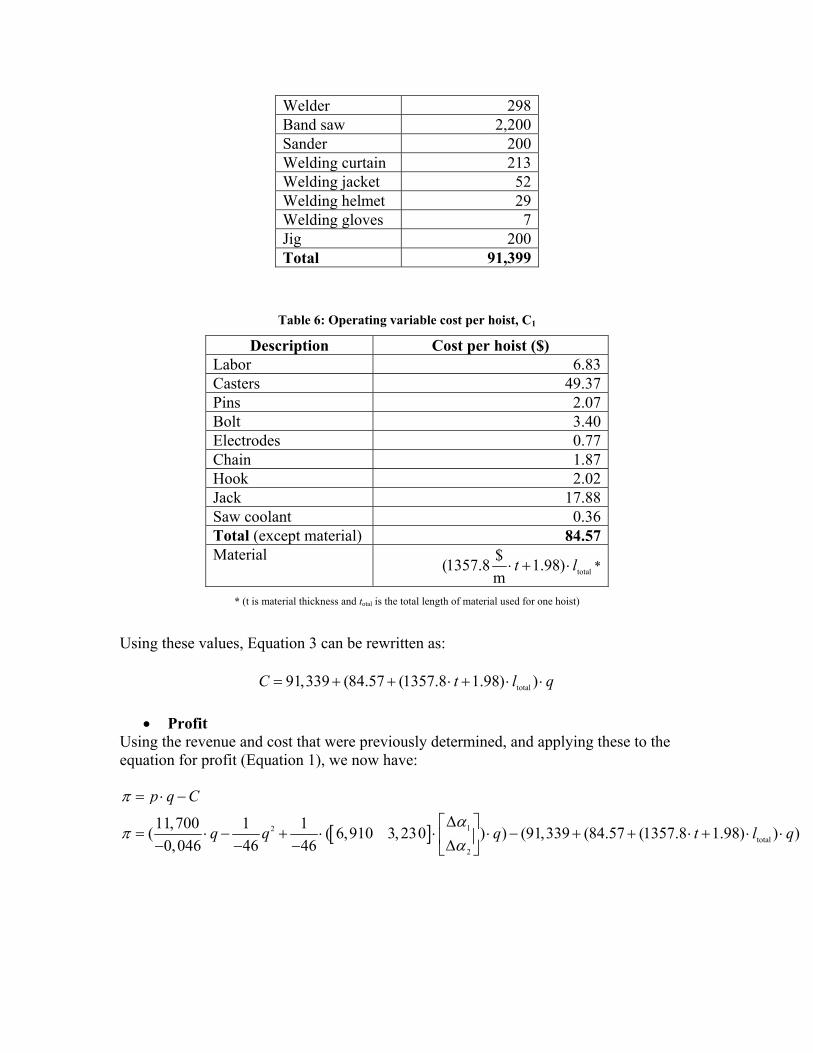
Welder 298Band saw 2,200Sander 200Welding curtain 213Welding jacket 52Welding helmet 29Welding gloves 7Jig 200Total 91,399
Table 6: Operating variable cost per hoist, C1
Description Cost per hoist ($) Labor 6.83 Casters 49.37 Pins 2.07 Bolt 3.40 Electrodes 0.77 Chain 1.87 Hook 2.02 Jack 17.88 Saw coolant 0.36 Total (except material) 84.57 Material
total
$(1357.8 1.98)m
t l⋅ + ⋅ *
* (t is material thickness and total is the total length of material used for one hoist)
Using these values, Equation 3 can be rewritten as:
total91,339 (84.57 (1357.8 1.98) )C t l q= + + ⋅ + ⋅ ⋅
• Profit Using the revenue and cost that were previously determined, and applying these to the equation for profit (Equation 1), we now have:
[ ] 12total
2
11,700 1 1( ( 6,910 3,230 ) ) (91,339 (84.57 (1357.8 1.98) ) )0,046 46 46
p q C
q q q t l q
πα
πα
= ⋅ −
∆ = ⋅ − + ⋅ ⋅ ⋅ − + + ⋅ + ⋅ ⋅ ∆− − −

3.3. Results Using the profit maximization function given above and applying it to the engineering model, the full economic model was created in Excel. As a result of using weight load and lifting capacity as design attributes however, certain items that had previously been simply calculated had to become variables. In addition, the design attributes, having once been parameters, had now to become intermediate variables. Table 7 below shows the new model that was obtained by running the optimization.
Table 7: Economic model
Maximize profitprofit = 1603017.382 dollars
Variables:h2 = 1.457 4.78 ftl6 = 0.867 2.85 ftalpha = 0.208 11.89 degl2 = 0.288 0.94 ftt = 0.017 0.68 ind = 0.102 4.00 inepsilon = 2.770 158.72 degF1 = 51750.042q = 20975.70851
Attributes:weight load = 5275.23362maximum height, h3 = 2.74 8.99 ft
An interesting thing to note about the results is that the optimal weight capacity is not 2 tons, as most hoists that are produced are designed for. In fact we arrived at a value closer to 5 tons. The cause of this is certainly the linear demand curve that was used for the attributes. In fact the demand for weight capacity is not linear, and after a certain capacity people no longer have any need for more. Regardless of the actual market need for the optimal solution, all values as they are considered together are quite reasonable.
4. Model Extension: Marketing
4.1. Market size To estimate the number of garages with an engine hoist in the U.S.A. we first identified the number of garages in Michigan using the Yellow Pages. To do the estimating we looked up “Auto Repair & Service” and added the number of garages which might own

an engine hoist, e.g. “Auto Customizing Services” and “Truck Repairs, General”. Using this method the number of garages with an engine hoist in Michigan is estimated to be 4,378. The population of Michigan (9,938,444) and the U.S.A. in total (292,598,364) was used to estimate the total number of garages in the U.S.A. which might own an engine hoist:
292,598,364 4,378 128,8939,938,444
⋅ =
Furthermore it is estimated that one out of 25,000 people in the U.S.A. own their own engine hoist. This means that 11,704 people own an engine hoist:
292,598,364 11,70425,000
=
The total number of engine hoists would then be 140,597. The number of engine hoists sold each year is estimated to be 14,060 assuming that an engine hoist is replaced every tenth year.
4.2. Determining betas It is assumed that there is a functional relationship between the product utility and the following three attributes: price (P), lifting height (LH) and load capacity (WL). A survey was conducted using an orthogonal array of 48 questions. This survey was then distributed to an upper level engineering class and the results compiled in excel. Using excel’s solver, the relative importance of each attribute was determined. The levels used in the analysis are shown below in Table 8, with the resulting beta coefficients shown in Table 9.
VALUES p z1 z2 $ WL LH 1 2 3
1 100 1 5
2 150 1.5 6
3 200 2 8 leve
l
4 250 2.5 9
Table 8: Levels of attributes in survey
BETAS
Price (beta 1)
Weight load (beta 2)
Lifting height (beta 3)

1 0.656 -1.666 -0.178
2 -0.059 -0.531 0.342
3 -1.184 0.427 1.638 leve
l
4 -1.974 0.81 1.537
Table 9: Solver returned beta coefficients
Using these beta coefficients and extrapolating to represent the continuous nature of the system, spline interpolation was used to develop plots of the three coefficients. These plots can be seen below in Figure 11, Figure 12, and Figure 13.
Beta 1
- 2.500
-2.000
-1.500
-1.000
-0.500
0.000
0.500
1.000
0 50 100 150 200 250 300
P r i c e - $
Figure 11: Beta for price
As would seem reasonable, the utility people have for a hoist is decreasing as price increases.
Beta 2
- 2.000
-1.500
-1.000
-0.500
0.000
0.500
1.000
0 0.5 1 1.5 2 2.5 3
L o a d c a p a c i t y - t o n
Figure 12: Beta for weight load
Interesting to note in the beta for weight load is the sharp increase of importance up to 2 tons. After this point the utility starts to taper off. This too seems quite reasonable, as few people have any need for the ability to lift more than 2 tons.

Beta 3
- 0.500
0.000
0.500
1.000
1.500
2.000
0 2 4 6 8 10
L i f t i n g h e i g h t - f t
Figure 13: Beta for lifting height
Finally, in the third beta we can see a sharp increase of importance as the lifting height increases to 8 ft. From this point on we then see the utility tapering off, reflecting the fact that most people only need a hoist that can lift up to 8 ft.
4.3. Linearized demand function, Qm With a baseline of $200, 2 tons, and 7’ the probability that people would purchase the hoist was found to be 58.6% using the spline function. This probability multiplied by the market size then gives a baseline quantity of q0 = 8,239. Holding two of the three attributes constant and taking a finite difference of the third, the change in probability was thus found for each attribute. These probabilities were found to be:
- Price, 51.7% → q1 = 7,269 - WL, 62.6% → q2 = 8,801 - LH, 65.2% → q3 = 9,167
Using these calculated quantities we thus found:
0 0( , ) 8, 239q P zθ = =v and
1 00
1
( ) 64.7p
q qqp h
λ −∂= = = −
∂
2 01 0
2 2
( ) 3,749q qqz h
λ −∂= = =
∂
3 02 0
3 3
( ) 2,320q qqz h
λ −∂= = =
∂
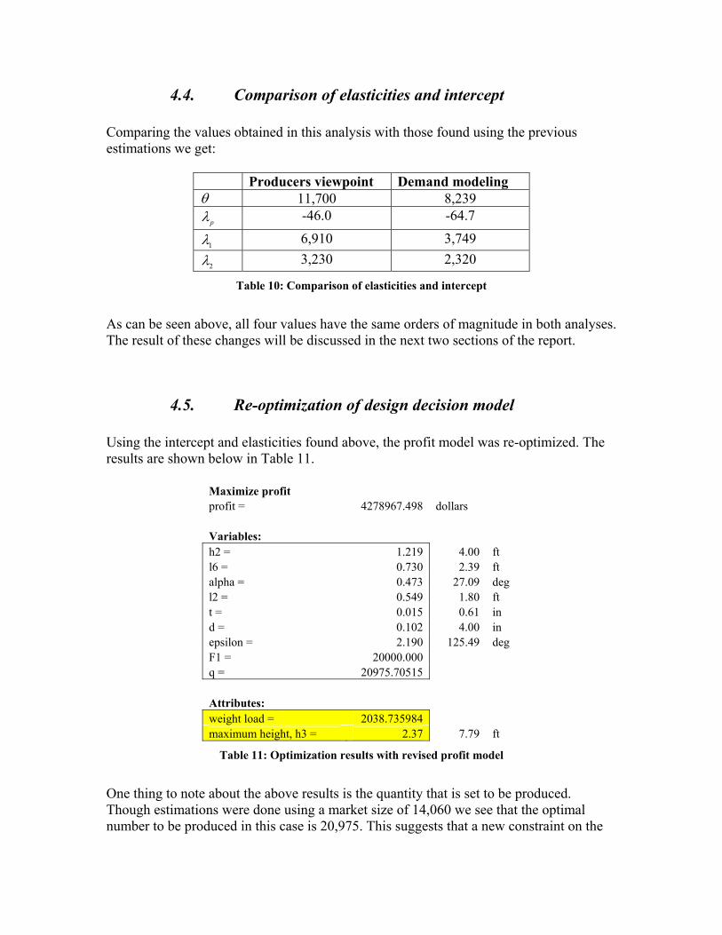
4.4. Comparison of elasticities and intercept Comparing the values obtained in this analysis with those found using the previous estimations we get:
Producers viewpoint Demand modeling θ 11,700 8,239
pλ -46.0 -64.7
1λ 6,910 3,749
2λ 3,230 2,320
Table 10: Comparison of elasticities and intercept
As can be seen above, all four values have the same orders of magnitude in both analyses. The result of these changes will be discussed in the next two sections of the report.
4.5. Re-optimization of design decision model Using the intercept and elasticities found above, the profit model was re-optimized. The results are shown below in Table 11.
Maximize profit profit = 4278967.498 dollars Variables: h2 = 1.219 4.00 ft l6 = 0.730 2.39 ft alpha = 0.473 27.09 deg l2 = 0.549 1.80 ft t = 0.015 0.61 in d = 0.102 4.00 in epsilon = 2.190 125.49 deg F1 = 20000.000 q = 20975.70515 Attributes: weight load = 2038.735984 maximum height, h3 = 2.37 7.79 ft
Table 11: Optimization results with revised profit model
One thing to note about the above results is the quantity that is set to be produced. Though estimations were done using a market size of 14,060 we see that the optimal number to be produced in this case is 20,975. This suggests that a new constraint on the

quantity should possibly be added to restrict the model. This was not done however so as to be able to compare the results to those from the previous optimization. Looking at the constraints we see:
Cell Name Cell Value Formula Status $B$43 Sigma,maxback = 3.0E+07 $B$43<=$G$28 Not Binding $B$40 Sigma,maxboom = 1.1E+08 $B$40<=$G$29 Not Binding $B$6 l6 = 0.730 $B$6<=$G$33 Not Binding $B$10 d = 0.102 $B$10>=$G$26 Not Binding $B$5 h2 = 1.219 $B$5<=$B$17 Not Binding $E$41 je^2 = l2^2 + l6^2 - 2l2l6cos(epsilon) 1.2996 $E$41=$G$41 Not Binding $E$38 ljc^2 = l2^2 + l6^2 - 2l2l6cos(tau) 0.3364 $E$38=$G$38 Not Binding $B$45 tau = 0.901 $B$45>=$G$36 Not Binding $B$9 t = 0.015 $B$9<=$G$25 Not Binding $B$9 t = 0.015 $B$9>=$G$24 Not Binding $B$10 d = 0.102 $B$10<=$G$27 Binding $B$8 l2 = 0.549 $B$8>=$G$30 Not Binding $B$7 alpha = 0.473 $B$7>=$G$32 Not Binding $B$8 l2 = 0.549 $B$8<=$G$31 Not Binding $B$5 h2 = 1.219 $B$5>=$G$35 Binding $B$13 q = 20975.70515 $B$13>=0 Not Binding $B$6 l6 = 0.730 $B$6>=$G$34 Not Binding
In this system we have nine variables, two equality constraints and two binding constraints. Since there are five degrees of freedom not accounted for this indicates that our system has found an interior solution and is not simply restricted by constraints. One interesting thing to note is that one of the binding constraints is the outer diameter of the tubing. Currently set to have a maximum value of 4”, this suggests that if more freedom were to be allowed in the diameter an even better solution might be found.
4.6. Comparison of results Looking at the values obtained from the two sets of optimizations, shown below in Table 12, we see changes in most of the variables. Those with differing values are highlighted. It should be noted that the profit found using the purely estimated intercept and elasticities is higher than that using the values obtained through survey data. These results suggest that the estimations made originally were simply too generous.
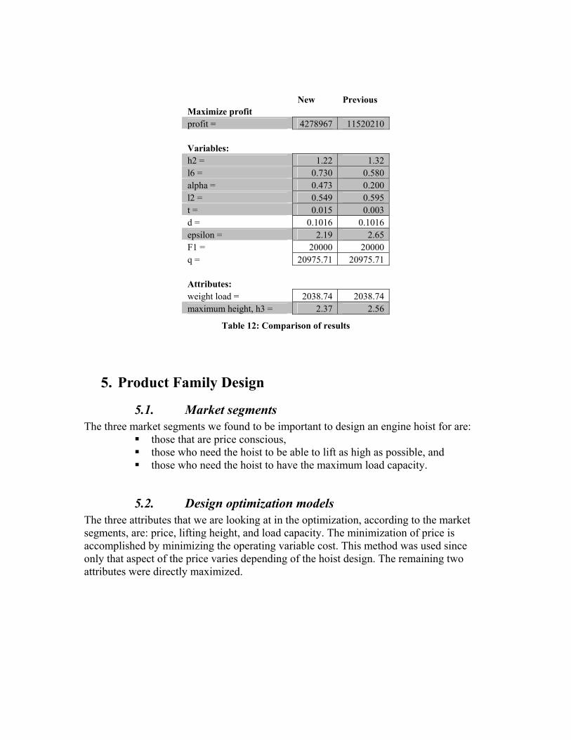
New Previous Maximize profit profit = 4278967 11520210 Variables: h2 = 1.22 1.32 l6 = 0.730 0.580 alpha = 0.473 0.200 l2 = 0.549 0.595 t = 0.015 0.003 d = 0.1016 0.1016 epsilon = 2.19 2.65 F1 = 20000 20000 q = 20975.71 20975.71 Attributes: weight load = 2038.74 2038.74 maximum height, h3 = 2.37 2.56
Table 12: Comparison of results
5. Product Family Design
5.1. Market segments The three market segments we found to be important to design an engine hoist for are:
those that are price conscious, those who need the hoist to be able to lift as high as possible, and those who need the hoist to have the maximum load capacity.
5.2. Design optimization models The three attributes that we are looking at in the optimization, according to the market segments, are: price, lifting height, and load capacity. The minimization of price is accomplished by minimizing the operating variable cost. This method was used since only that aspect of the price varies depending of the hoist design. The remaining two attributes were directly maximized.

5.3. Separate design optimizations
a. Load capacity Variables Parameters F1, l2, l6 d, t g, A Objective
1max Fg
Secondary equations
max 1 2( )boomM F A l= −
maxmax
boomboom
M yI
σ ⋅=
4 42
( 2 )12 12
dy
d d tI
=
−= −
2max ,
1,
max max , ,
cos( )
back M
back t
back back M back t
M yI
Fa
σ
ασ
σ σ σ
⋅=
⋅=
= +
12 6 1
2
2
2 2
sin( ) sin( )
cos( )( )
b
b
F AM l F ll
hl
a d d t
α α
α
⋅= ⋅ ⋅ + ⋅ ⋅
=
= − −
Constraints
1 2
2 2
3 6
4 6
5
6 2
7
8
9
10
811 max
812 max
0.127 00.65 0
0.58 01.236 0
0.2 01.219 00.0016 0
0.5( ) 02( ) 0
0.1016 0
3.7 10 0
3.7 10 0boom
back
g lg lg lg lgg hg tg t dg t dg d
g
g
α
σ
σ
= − ≤= − ≤= − ≤= − ≤= − ≤= − ≤= − ≤= − ≤= − ≤= − ≤
= − × ≤
= − × ≤
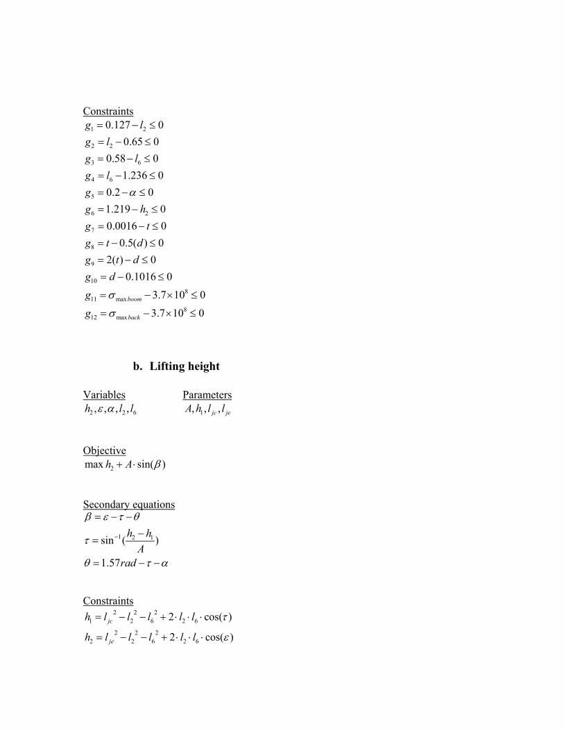
b. Lifting height Variables Parameters
2 2 6, , , ,h l lε α 1, , ,jc jeA h l l Objective
2max sin( )h A β+ ⋅ Secondary equations
1 2 1sin ( )
1.57
h hA
rad
β ε τ θ
τ
θ τ α
−
= − −−
=
= − −
Constraints
2 2 21 2 6 2 6
2 2 22 2 6 2 6
2 cos( )
2 cos( )jc
je
h l l l l l
h l l l l l
τ
ε
= − − + ⋅ ⋅ ⋅
= − − + ⋅ ⋅ ⋅

1 2
2 2
3 6
4 6
5
6 2
7
8
9
10
811 max
812 max
0.127 00.65 0
0.58 01.236 0
0.2 01.219 00.0016 0
0.5( ) 02( ) 0
0.1016 0
3.7 10 0
3.7 10 0boom
back
g lg lg lg lgg hg tg t dg t dg d
g
g
α
σ
σ
= − ≤= − ≤= − ≤= − ≤= − ≤= − ≤= − ≤= − ≤= − ≤= − ≤
= − × ≤
= − × ≤
c. Price (operating variable cost) Variables Parameters
2, ,t h α A Objective min84.57 (1357.8 1.98) tt l+ ⋅ + ⋅ Secondary equations
2
3( )
cos( )
t b
b
l A l Ahlα
= + +
=
Constraints
1 2
2 2
3 6
4 6
5
6 2
7
8
9
10
0.127 00.65 0
0.58 01.236 0
0.2 01.219 00.0016 0
0.5( ) 02( ) 0
0.1016 0
g lg lg lg lgg hg tg t dg t dg d
α
= − ≤= − ≤= − ≤= − ≤= − ≤= − ≤= − ≤= − ≤= − ≤= − ≤

5.4. Creating Pareto surface with first set of commonality constraints
The first commonality constraint that was imposed on the model was for the value of the length of the hoist back. The data associated with the weights that were selected is shown below in Table 13. maximum height = 2.550 2.6 2.64 2.6 2.63 2.63 2.64 2.64 2.56 2.63 2.64 2.64 2.61 2.64 2.6 2.58 2.62 2.64 2.64 2.64Load capacity = 2.040 8.84 2.04 6.63 6.63 6.12 6.12 6.12 5.61 5.1 5.1 5.1 7.65 7.65 7.65 2.04 2.04 2.04 2.04 2.04Variable cost = 204 884 204 663 663 612 612 612 561 510 510 510 765 765 765 204 204 204 204 204
W_height 0 0 1 0.1 0.2 0.3 0.4 0.5 0.15 0.3 0.45 0.6 0.1 0.2 0.3 0.1 0.3 0.5 0.7 0.9W_load 0 1 0 0.5 0.5 0.5 0.5 0.5 0.3 0.3 0.3 0.3 0.7 0.7 0.7 0.1 0.1 0.1 0.1 0.1W_cost 1 0 0 0.4 0.3 0.2 0.1 0 0.55 0.4 0.25 0.1 0.2 0.1 0 0.8 0.6 0.4 0.2 0
Table 13: Data for first set of commonality constraints
Since it was not possible to create a useful 3-D plot of the data, the three respective 2-D plots are shown below in Figure 14 through Figure 16.
Lifting height vs. Load capacity
0
1
2
3
4
5
6
7
8
9
10
2.540 2.560 2.580 2.600 2.620 2.640 2.660
Lifting height (m)
Load
cap
acity
(ton
s)
Figure 14: 2D pareto curve for lifting height vs. load capacity

Lifting height vs. Variable cost
0.00
50.00
100.00
150.00
200.00
250.00
300.00
350.00
2.540 2.560 2.580 2.600 2.620 2.640 2.660
Lifting height (m)
Varia
ble
cost
($)
Figure 15: 2D pareto curve for lifting height vs. variable cost
Load capacity vs. Variable cost
0.00
50.00
100.00
150.00
200.00
250.00
300.00
350.00
0 2 4 6 8 10
Load capacity (tons)
Varia
ble
cost
($)
Figure 16: 2D pareto curve for load capacity vs. variable cost

5.5. Pareto surface with second set of commonality constraints
The second commonality constraint imposed on the model was the thickness of the material. Again, the data is shown below in Table 14, and the respective 2-D plots below in Figure 17 through Figure 19. maximum height = 2.550 2.6 2.64 2.6 2.63 2.63 2.64 2.64 2.56 2.63 2.64 2.64 2.61 2.64 2.6 2.58 2.62 2.64 2.64 2.64Load capacity = 2.040 8.84 2.04 6.63 6.63 6.12 6.12 6.12 5.61 5.1 5.1 5.1 7.65 7.65 7.65 2.04 2.04 2.04 2.04 2.04Variable cost = 125 547 387 229 229 221 214 460 179 179 169 169 268 268 453 125 125 126 126 387
W_height 0 0 1 0.1 0.2 0.3 0.4 0.5 0.15 0.3 0.45 0.6 0.1 0.2 0.3 0.1 0.3 0.5 0.7 0.9W_load 0 1 0 0.5 0.5 0.5 0.5 0.5 0.3 0.3 0.3 0.3 0.7 0.7 0.7 0.1 0.1 0.1 0.1 0.1W_cost 1 0 0 0.4 0.3 0.2 0.1 0 0.55 0.4 0.25 0.1 0.2 0.1 0 0.8 0.6 0.4 0.2 0
Table 14: Data for second set of commonality constraints
Lifting height vs. Load capacity
0
2
4
6
8
10
12
2.590 2.600 2.610 2.620 2.630 2.640 2.650
Lifting height (m)
Load
cap
acity
(ton
s)
Figure 17: 2D Pareto curve for lifting height vs. load capacity

Lifting height vs. Variable cost
0
100
200
300
400
500
600
2.590 2.600 2.610 2.620 2.630 2.640 2.650
Lifting height (m)
Varia
ble
cost
($)
Figure 18: 2D Pareto curve for lifting height vs. variable cost
Load capacity vs. Variable cost
0
100
200
300
400
500
600
0 2 4 6 8 10 12
Load capacity (tons)
Varia
ble
cost
($)
Figure 19: 2D Pareto curve for load capacity vs. variable cost
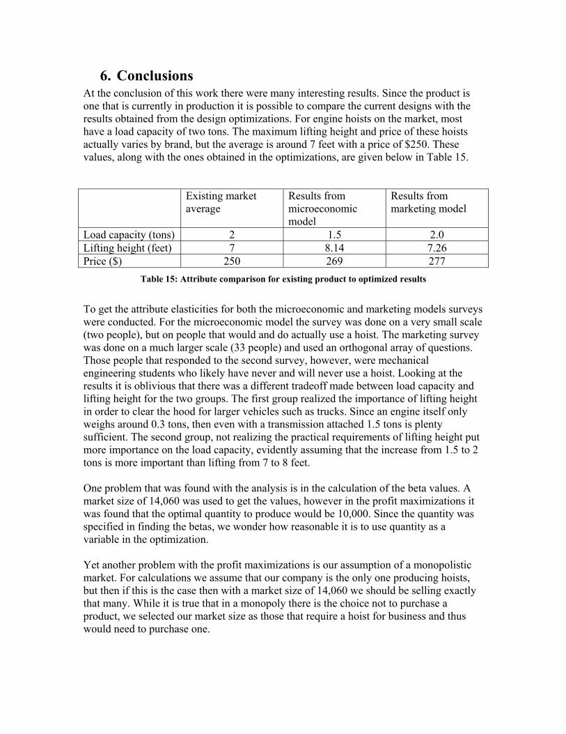
6. Conclusions At the conclusion of this work there were many interesting results. Since the product is one that is currently in production it is possible to compare the current designs with the results obtained from the design optimizations. For engine hoists on the market, most have a load capacity of two tons. The maximum lifting height and price of these hoists actually varies by brand, but the average is around 7 feet with a price of $250. These values, along with the ones obtained in the optimizations, are given below in Table 15. Existing market
average Results from microeconomic model
Results from marketing model
Load capacity (tons) 2 1.5 2.0 Lifting height (feet) 7 8.14 7.26 Price ($) 250 269 277
Table 15: Attribute comparison for existing product to optimized results
To get the attribute elasticities for both the microeconomic and marketing models surveys were conducted. For the microeconomic model the survey was done on a very small scale (two people), but on people that would and do actually use a hoist. The marketing survey was done on a much larger scale (33 people) and used an orthogonal array of questions. Those people that responded to the second survey, however, were mechanical engineering students who likely have never and will never use a hoist. Looking at the results it is oblivious that there was a different tradeoff made between load capacity and lifting height for the two groups. The first group realized the importance of lifting height in order to clear the hood for larger vehicles such as trucks. Since an engine itself only weighs around 0.3 tons, then even with a transmission attached 1.5 tons is plenty sufficient. The second group, not realizing the practical requirements of lifting height put more importance on the load capacity, evidently assuming that the increase from 1.5 to 2 tons is more important than lifting from 7 to 8 feet. One problem that was found with the analysis is in the calculation of the beta values. A market size of 14,060 was used to get the values, however in the profit maximizations it was found that the optimal quantity to produce would be 10,000. Since the quantity was specified in finding the betas, we wonder how reasonable it is to use quantity as a variable in the optimization. Yet another problem with the profit maximizations is our assumption of a monopolistic market. For calculations we assume that our company is the only one producing hoists, but then if this is the case then with a market size of 14,060 we should be selling exactly that many. While it is true that in a monopoly there is the choice not to purchase a product, we selected our market size as those that require a hoist for business and thus would need to purchase one.

7. Appendices
5.1. Appendix A: Patent images


7.2. Appendix B: Initial fixed investment and variable cost Initial fixed investment
Description See comment #
See appendix #
Cost per year ($)
Warehouse 1 12,000 Utilities 2 1,200 Salary 3 75,000 Welder 4 1 298 Band saw 5 2 2,200 Sander 6 3 200 Welding curtain 7 213 Welding jacket 8 52 Welding helmet 9 29 Welding gloves 10 7 Jig 11 200 Total 91,399
Comment #:
1. It is estimated that warehouse cost $1,000 per month. 2. It is estimated that utilities cost $100 per month. 3. It is estimated that the salary for the boss/foreman would be $75,000 per year. 4. It is estimated that one welder is needed. The price of a welder is (see appendix 1)
$298. 5. It is estimated that one band saw is needed. The price of a band saw is (see
appendix 2) $2,200. 6. It is estimated that one sander is needed. The price of a sander is (see appendix 3)
$200. 7. Price of a 4x6 – 3 panels curtain is $213 according to Ann Arbor Welding Supply. 8. Price of a XL leather jacket is $52 according to Ann Arbor Welding Supply. 9. Price of a helmet with standard lenses is $29 according to Ann Arbor Welding
Supply. 10. Price of leather gloves size L $7 according to Ann Arbor Welding Supply. 11. It is estimated that material and labor to make the jig would cost $200.

Operating variable cost per hoist
Description See comment #
See appendix #
Cost per hoist ($)
Labor 12 12 6.83Casters 13 4 and 5 49.37Pins 14 6 2.07Bolt 15 7 3.40Electrodes 16 0.77Chain 17 9 1.87Hook 18 10 2.02Jack 19 11 17.88Saw coolant 20 13 0.36Total (except material) 84.57Material 21
total
$(1357.8 "thickness" 1.98)m
l⋅ + ⋅
Comment #:
12. Based on appendix 12 the hourly labor cost is estimated to $ 1.11: $2,313
$year 1.11week hour hour52 40year week
=⋅
and it is estimated that is takes 6.15 hours to make
one hoist (2.8 hours to machine, 2.6 hours to weld, 0.75 hours to assembly). Thereby the labor cost is approximately $6.83.
13. It is necessary to use 6 casters in total. The four has to carry the hoist when loaded and the two only when it is stored and not carry any load. The price for the casters can be found in appendix 4 and 5 to be $22.82 and $37.96 for the two and the four casters respectably. It is estimated that buying a lot of casters it is possible to get a 75% rebate. Thereby the price for the casters become: 0.25 (2 $22.82 4 $37.96) 49.37⋅ ⋅ + ⋅ .
14. It is necessary to use 2 pins in total. The price of pins is found in appendix 6 to be $4.14. Again it is estimated that it is possible to get a 75% rebate. The price for pins is: 0.25 (2 $4.14) $2.07⋅ ⋅ .
15. It is necessary to use 3 bolts in total. The price of bolts is found in appendix 7 to be $4.53. With the estimated rebate the price for the bolts is: 0.25 (3 $4.53) $3.40⋅ ⋅ .
16. The price of a 5lb box of 6013 1/8” electrodes is $9.25 according to Ann Arbor Welding. It is estimated that one box will last for 12 hoists and the price for electrodes to one hoist is $0.77.

17. The price of a welded chain is found to be $7.45 per foot (see appendix 9). The rebate is in this situation estimated to 50% and it is estimated the each hoist need a chain of ½ a food. The price is therefore: 0.5 0.5 $7.45 $1.87⋅ ⋅ .
18. The price of a hook is found to be $8.09 (see appendix 10). A rebate of 75% is estimated. The price is: 0.25 $8.09 $2.02⋅ = .
19. The price of a bottle jack is found in appendix 11 to be $35.75. Here a rebate of 50% is estimated and the price is $17.88.
20. The price of one gallon of saw coolant is $35.95 (see appendix 13) and is estimated to last for 100 hoists. The price for one hoist is: $0.36.
21. The price of material with three different thicknesses was collected from …. To get material price as a function of thickness a regression was done (see Figure 20)
and the following function found: material $1357.8 "thickness" 1.98m m
p= ⋅ + .
Multiplying with the total length needed the price for material per hoist is:
material total
$(1357.8 "thickness" 1.98)m
p l= ⋅ + ⋅
Material pricey = 1357.8x + 1.9797
0
1
2
3
4
5
6
7
8
9
0 0.001 0.002 0.003 0.004 0.005 0.006
Thickness (m)
Pric
e Series1Linear (Series1)
Figure 20: Metal price as a function of thickness

Business plan
A) Business opportunity
a) Business objective The goal of this company is to produce engine hoists. In particular it is intended that the hoists be of good quality, low cost, and have good profit margins. As with any other company going into business the end goal is to make money, however the intent here is to use financial and engineering tools to make that money while producing an appealing and quality product. In this way, the plan is to optimize profit while considering the product price, produced quantity and product attribute variables.
b) Product description The intended users of this product are both commercial garages and private at-home mechanics. For these users, the engine hoist should be designed such that dimensions are chosen that minimize weight. In this way the hoist should be easy to move around, but should also retain its required functionality in load capacity. In addition, the design should have an acceptable range of operating angles to accommodate the change in vertical height required by the user. The product should also fold up into a more compact form and should be easy to operate. Finally, it is important that the product be inexpensive and the load capacity able to be changed by adjusting the length of the boom. In summary,
• The product must be able to lift a specified range of loads. • The boom must be long enough to reach and support the load (clearance issues). • Using an existing hydraulic ram, the product must be able to move through a
specified range of operating heights. • The total weight should be minimal such that it can easily be moved around. • The appearance of the product must be appealing. • The cost of the produce must be minimal. • The product should be able to fold up into a smaller volume for ease of storage
and transportation. • The load capacity of the hoist should be able to be changed by adjusting the
length of the boom.

c) Market analysis To estimate the number of garages with an engine hoist in the U.S.A. we first identified the number of garages in Michigan using the Yellow Pages. To do the estimating we looked up “Auto Repair & Service” and added the number of garages which might own an engine hoist, e.g., “Auto Customizing Services” and “Truck Repairs, General”. Using this method the number of garages with an engine hoist in Michigan is estimated to be 4,378. The population of Michigan (9,938,444) and the U.S.A. in total (292,598,364) was used to estimate the total number of garages in the U.S.A. which might own an engine hoist:
292,598,364 4,378 128,8939,938,444
⋅ =
Furthermore it is estimated that one out of 25,000 people in the U.S.A. own their own engine hoist. This means that 11,704 people own an engine hoist:
292,598,364 11,70425,000
=
The total number of engine hoists would then be 140,597. The number of engine hoists sold each year is thus estimated to be 14,060 assuming that an engine hoist is replaced every tenth year. To determine what percentage of this total our particular company should produce, a profit optimization was done. The market analysis was developed around results of a survey. From the optimization we were then able to obtain the ideal values for our design attributes. Using these values and the spline interpolation of our market data this told us that for our design, in a monopoly, we would have a market share of 35.8%. Table 16 below shows these values.
Table 16: Market share prediction for given attributes
p z1 z2 Sum(BETA) Pr val 277 2.04 7.26 beta -2.357 0.477 1.293 -0.586 35.8%
For an overall market of 14,060, a 35.8% market share translates to an annual production of 5,033 units.

B) Financial data
a) Capital equipment and supply list The initial costs associated with purchasing an engine hoist are given below in Table 17. The annual operating costs are then given in Table 18 with the operating variable costs given in Table 6.
Table 17: Initial fixed investments
Description Cost per year ($) Welder 298Band saw 2,200Sander 200Welding curtain 213Welding jacket 52Welding helmet 29Welding gloves 7Jig 200Total $3,199
Table 18: Annual operating costs without cost of production
Description Cost per year ($) Warehouse 12,000Utilities 1,200Salary 75,000Total $88,200
Table 19: Operating variable cost per hoist
Description Cost per hoist ($) Labor 6.83 Casters 49.37 Pins 2.07 Bolt 3.40 Electrodes 0.77 Chain 1.87 Hook 2.02 Jack 17.88 Saw coolant 0.36 Material 56.29 Total $140.86

To determine the overall annual operating costs, the costs associated with maintaining a facility and staff was combined with the overall cost of producing the 5,033 units. In other words the cost would be:
88,200 (140.86 5,033) 797,148.38+ ⋅ = The salvage cost was then estimated as being 50% of the new price of the machinery. The other welding accessories have no salvage value. This gives us a salvage of:
(298 2,200 200) 0.50 1,349+ + ⋅ = The overall economic data can then be summarized as shown in Table 20.
Table 20: Economic data
First cost 3,199Annual operating cost 797,148Annual income 1,394,141Salvage value 1,349
b) Breakeven analysis To determine the breakeven point for hoist production, the following equation was used:
(First cost) + (Operating cost) = (Annual income) + (Return from salvage) This can also be given as:
(1 )3,199 797,148 1,394,141 1,349(1 ) 1 (1 ) 1
n
n n
i i ii i
+⋅ + = + ⋅ + − + −
If we take i = 6% as the interest rate and solve the above equation for the number of periods we get the results shown below in Table 21.
Table 21: Breakeven point
Engine hoist Investment -800347Yearly Profit 1394141Salvage 1349 Periods 0.60055 PV Profit $799,044.39 PV Salvage $1,302.61 Difference $0.00
Thus, since it would take less than a year to make back the initial investment, the manufacturing of engine hoists would seem to be quite a profitable endeavor.
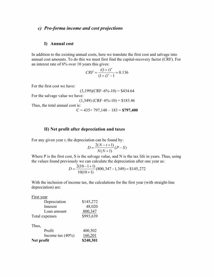
c) Pro-forma income and cost projections
I) Annual cost In addition to the existing annual costs, here we translate the first cost and salvage into annual cost amounts. To do this we must first find the capital-recovery factor (CRF). For an interest rate of 6% over 10 years this gives:
(1 ) 0.136(1 ) 1
n
n
i iCRFi+
= =+ −
For the first cost we have:
(3,199)(CRF–6%-10) = $434.64 For the salvage value we have:
(1,349) (CRF–6%-10) = $183.46 Thus, the total annual cost is:
C = 435+ 797,148 – 183 = $797,400
II) Net profit after depreciation and taxes For any given year t, the depreciation can be found by:
2( 1) ( )( 1)
N tD P SN N
− += −
+
Where P is the first cost, S is the salvage value, and N is the tax life in years. Thus, using the values found previously we can calculate the depreciation after one year as:
2(10 1 1) (800,347 1,349) $145,27210(10 1)
D − += − =
+
With the inclusion of income tax, the calculations for the first year (with straight-line depreciation) are: First year
Depreciation $145,272 Interest 48,020 Loan amount 800,347
Total expenses $993,639 Thus, Profit 400,502 Income tax (40%) 160,201 Net profit $240,301

C) Supporting documents
a) Existing patents The abstract for the engine hoist patent is given below, with the patent information given in Figure 7.
“A portable engine hoist which folds into a compact storage position. The base of the hoist is equipped with two support wheels. Two elongated legs extend from the base and are adapted to receive leg extensions. The leg extensions are provided with wheels at one end and the other end can be inserted into a leg. An upright post extends from a base support and carries a pivotally mounted lifting beam at its top end. A mechanical or hydraulic jack operates to raise and lower the lifting beam to raise and lower an engine. Position adjustment and maintenance means for easy assembly of the leg extensions are provided. A cam slot locking means associated with the lifting beam provides stability under the load”.

Figure 21: Engine hoist patent

b) Technical analysis and benchmarking In addition to the analysis that was done with one particular configuration of an engine hoist, other designs were also investigated. Some of the different designs are shown below.

8. Slut