design for transmission systems

UNIVERSITY OF SOUTHERN MINDANAOCOLLEGE OF ENGINEERING AND COMPUTING

DEPARTMENT OF ELECTRONICS ENGINEERING

DESIGNING OF A CABLE TV SYSTEM IN HOUSEHOLDS

SUBMITTED BY:

LONGAKIT, TRIXIA ANGELIE P.

JOHN ROYCE BAYOTLANG

FRANCIS RAGIB MANTAWIL

ROMMEL MORIDO

SUBMITTED TO:

ENGR. GERALDO P. ULEP, PECE

CABLE TV SYSTEM

Terrestrial, satellite, and cable - these are the classic means of transmission for TV

broadcasting. Each of them uses different technologies with respect to modulation, forward error

correction, and system design adapted to the specific environment. Digital cable TV

broadcasting utilizes single carrier quadrature amplitude modulation (QAM) with typically 16, 64,

256, 512, and now also 1024 valence. In the past, three main standards were implemented in

different regions of the world. The three standards have been consolidated in Recommendation

J.83 by the Telecommunication Standardization Sector of the International Telecommunication

Union (ITU-T). To deliver the television signal to consumer households via cable, a reliable

distribution system is required.

A cable headend is responsible for conditioning the actual RF signal that is output.

Satellite, IP link, or directional radio are typically used to supply the headend with the digital

video and audio data for the various television services. Mainly delivered as an MPEG-2

transport stream, the baseband feed depends on the requirements remultiplexed and input to

the different modulators. A system combiner is used to merge all modulated channels to a

single output for further distribution over the cable network.

Conventional coaxial cables are used to transmit this single output signal to consumer

households. A signal carried over these copper cables is attenuated due to cable loss. To

ensure that all cable service subscribers over a wide area are provided with signals of sufficient

level, amplification needs to be performed along the transmission path. The rule of thumb here

is one amplifier every 300 meters.

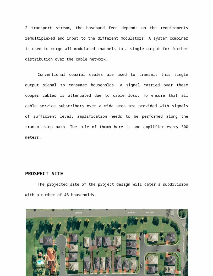
PROSPECT SITE

The projected site of the project design will cater a subdivision with a number of 46

households.

DISTRIBUTION

In order to receive cable television at a given location, cable distribution lines

must be available on the local utility poles or underground utility lines. Coaxial cable brings the

signal to the customer's building through a service drop, an overhead or underground cable. If

the subscriber's building does not have a cable service drop, the cable company will install one.

The standard cable used in the U.S. is RG-6, which has a 75 ohm impedance, and connects

with a type F connector. coax cable has a bandwidth in the hundreds of megahertz, which is

more than enough to transmit multiple streams of video and audio simultaneously. The cable

wire transmits every single channel, simultaneously. It does this by using frequency division

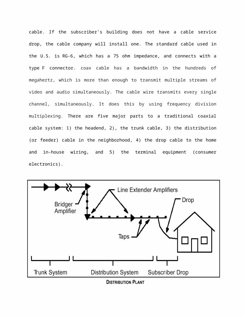
multiplexing. There are five major parts to a traditional coaxial cable system: 1) the headend, 2),

the trunk cable, 3) the distribution (or feeder) cable in the neighborhood, 4) the drop cable to the

home and in-house wiring, and 5) the terminal equipment (consumer electronics).

https://en.wikipedia.org/wiki/F_connector

https://en.wikipedia.org/wiki/RG-6

https://en.wikipedia.org/wiki/Service_drop

https://en.wikipedia.org/wiki/Coaxial_cable

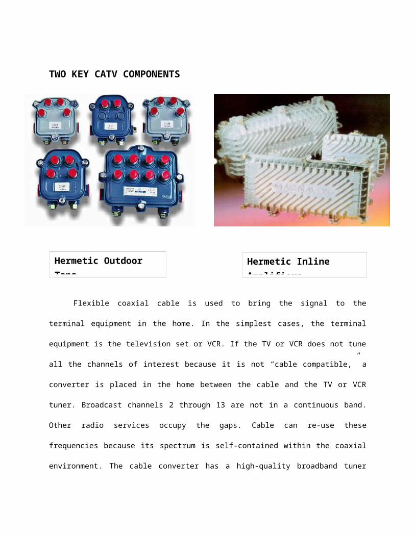
TWO KEY CATV COMPONENTS

Flexible coaxial cable is used to bring the signal to the terminal equipment in the home.

In the simplest cases, the terminal equipment is the television set or VCR. If the TV or VCR

does not tune all the channels of interest because it is not “cable compatible,” a converter is

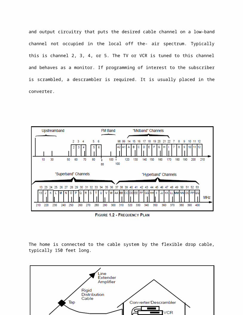
placed in the home between the cable and the TV or VCR tuner. Broadcast channels 2 through

13 are not in a continuous band. Other radio services occupy the gaps. Cable can re-use these

frequencies because its spectrum is self-contained within the coaxial environment. The cable

converter has a high-quality broadband tuner and output circuitry that puts the desired cable

channel on a low-band channel not occupied in the local off the- air spectrum. Typically this is

channel 2, 3, 4, or 5. The TV or VCR is tuned to this channel and behaves as a monitor. If

programming of interest to the subscriber is scrambled, a descrambler is required. It is usually

placed in the converter.

Hermetic Outdoor Taps Hermetic Inline Amplifiers

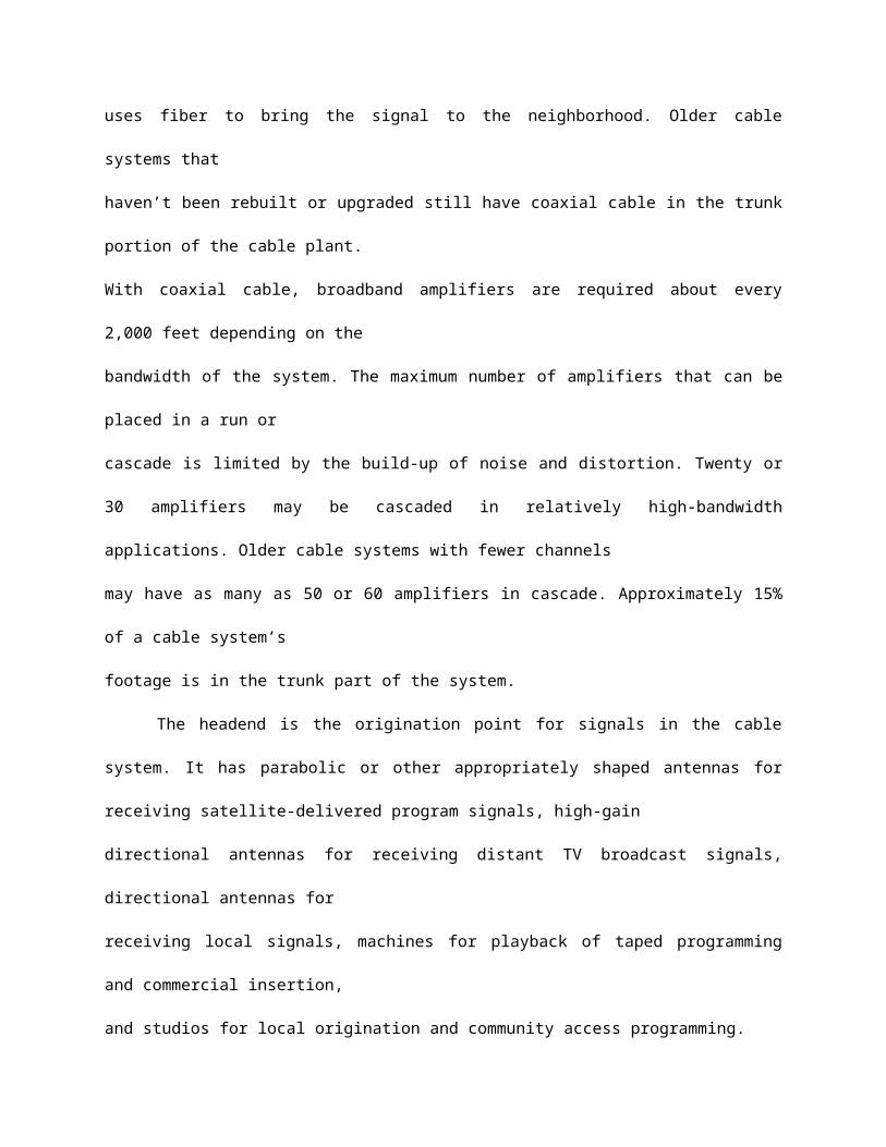
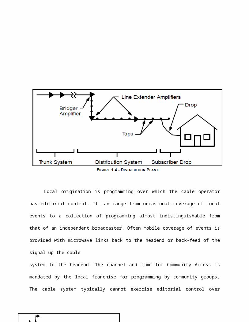
The home is connected to the cable system by the flexible drop cable, typically 150 feet long.

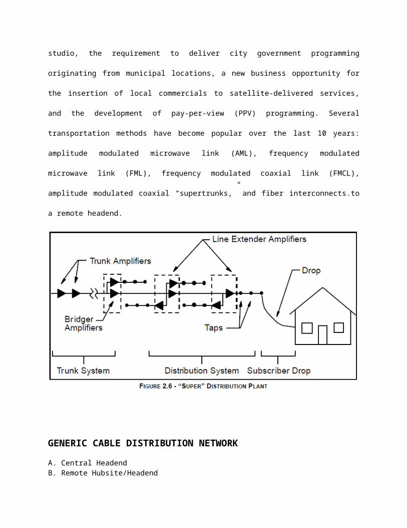
The distribution cable in the neighborhood runs past the homes of subscribers. This

cable is tapped so that flexible drop cable can be connected to it and routed to the residence.

The distribution cable interfaces with the trunk cable through an amplifier called a Bridger

amplifier, that increases the signal level for delivery to multiple homes. One or two specialized

amplifiers, called line extenders, are included in each distribution cable. Approximately 40% of

the system’s cable footage is in the distribution portion of the plant and 45% is in the flexible

drops to the home.

The trunk part of the cable system transports the signals to the neighborhood. Its

primary goal is to cover distance while preserving the quality of the signal in a cost-effective

manner. Current practice uses fiber to bring the signal to the neighborhood. Older cable

systems that

haven’t been rebuilt or upgraded still have coaxial cable in the trunk portion of the cable plant.

With coaxial cable, broadband amplifiers are required about every 2,000 feet depending on the

bandwidth of the system. The maximum number of amplifiers that can be placed in a run or

cascade is limited by the build-up of noise and distortion. Twenty or 30 amplifiers may be

cascaded in relatively high-bandwidth applications. Older cable systems with fewer channels

may have as many as 50 or 60 amplifiers in cascade. Approximately 15% of a cable system’s

footage is in the trunk part of the system.

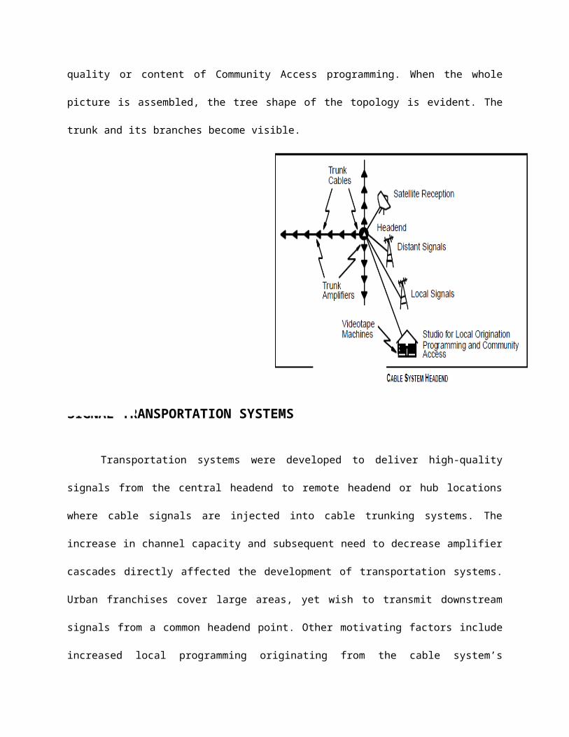
The headend is the origination point for signals in the cable system. It has parabolic or

other appropriately shaped antennas for receiving satellite-delivered program signals, high-gain

directional antennas for receiving distant TV broadcast signals, directional antennas for

receiving local signals, machines for playback of taped programming and commercial insertion,

and studios for local origination and community access programming.

Local origination is programming over which the cable operator has editorial control. It

can range from occasional coverage of local events to a collection of programming almost

indistinguishable from that of an independent broadcaster. Often mobile coverage of events is

provided with microwave links back to the headend or back-feed of the signal up the cable

system to the headend. The channel and time for Community Access is mandated by the local

franchise for programming by community groups. The cable system typically cannot exercise

editorial control over quality or content of Community Access programming. When the whole

picture is assembled, the tree shape of the topology is evident. The trunk and its branches

become visible.

SIGNAL TRANSPORTATION SYSTEMS

Transportation systems were developed to deliver high-quality signals from the central

headend to remote headend or hub locations where cable signals are injected into cable

trunking systems. The increase in channel capacity and subsequent need to decrease amplifier

cascades directly affected the development of transportation systems. Urban franchises cover

large areas, yet wish to transmit downstream signals from a common headend point. Other

motivating factors include increased local programming originating from the cable system’s

studio, the requirement to deliver city government programming originating from municipal

locations, a new business opportunity for the insertion of local commercials to satellite-delivered

services, and the development of pay-per-view (PPV) programming. Several transportation

methods have become popular over the last 10 years: amplitude modulated microwave link

(AML), frequency modulated microwave link (FML), frequency modulated coaxial link (FMCL),

amplitude modulated coaxial “supertrunks,” and fiber interconnects.to a remote headend.

GENERIC CABLE DISTRIBUTION NETWORK

A. Central HeadendB. Remote Hubsite/HeadendC. AML Microwave LinkD.FML Microwave LinkE. Supertrunk AmplifierF. Supertrunk Cable and ConnectorsG. Trunk AmplifierH. Trunk Cable and ConnectorsJ. Line SplittersK. Line ExtenderL. Distribution Cable and ConnectorsM. MultitapN. Indoor SplittersP. Subscriber Drop Cable and ConnectorsQ. ConverterR. Video Cassette RecorderS.Television

A - CENTRAL HEADEND

The central headend is the main signal reception, origination, and modulation point for

thecable system. It performs the following functions:

• Receives satellite programming via Television Receive Only (TVRO) sites

• Receives off-air broadcasts of television and radio

• Receives distant signals by FML microwave or return band cable

• Modulates programming onto channel assignments for distribution (up to 80 channels)

• FM modulates video for remote headend

• Performs local advertising insertion

• Inserts channels into trunk system.

Characteristics of Equipment

The basic TVRO station consists of an antenna, a low-noise amplifier (LNA) or low

noise block converter (LNB), an FM receiver, and interconnecting cable. The LNA, typically

attached directly to the antenna, accepts the incoming downlink signal from the antenna and

amplifies this signal for input to the receiver. The downlink frequencies in use are in two bands

the C band (3.7 to 4.2 GHz) and the Ku band (10.95 to 14.5 GHz) – each of which is broken into

smaller sub-bands. The LNB not only amplifies, but also down converts the entire band to UHF

or L-band frequencies. TVRO parabolic antennas are available in various sizes (2.8 to 10 m

diameter) depending on the required gain. The antennas are adjusted to focus on a

geosynchronous satellite to receive the available channels. The receiver converts the downlink

frequencies to UHF frequencies either one channel at a time or in a block and provides a signal

ready for modulation onto the cable system.

Typical Receiver Specifications

RF Input

Maximum Level - 34 dBm

Frequency Range 3.7 to 4.2 GHz

Characteristic Impedance 50 ohms

Return Loss > 20 dB

Noise Figure 15 dB maximum

Image Rejection > 60 dB

LO Leakage < - 70 dBm

IF

Intermediate Frequency 70 MHz

Effective Noise Bandwidth 32.4 MHz


Return Loss at IF Monitor Ports > 20 dB

Dynamic Operating Range 40 dB

Baseband

De-emphasis 525-line CCIR Rec. 405-1

Deviation range 6 to 12 MHz peak at de-emphasis crosssover frequency

FM Video Static Threshold 8 dB carrier-to-noise ratio with thresholdextension demodulation (TED)

Video Level 1 V p-p ± 3 dB

Response (15 Hz - 4.2 MHz) Standard: ± 0.5 dB ± 1.0 dB with TED


Return Loss > 26 dB

Polarity Black to White: Positive going

Clamping 40 dB dispersal rejection

Line-Time Waveform Distortion < 1% tilt

Field-Time Waveform Distortion < 1% tilt

Differential Phase < ± 1°: 10 to 90% APL

Differential Gain < ± 2.5%: 10 to 90% APL

Audio

Subcarrier Frequency 6.8 MHz

Frequency Response 30 Hz to 15 kHz ± 0.5 dB

De-Emphasis 75 μs

Output Level Range - 10 to + 10 dBm


Harmonic Distortion < 1%

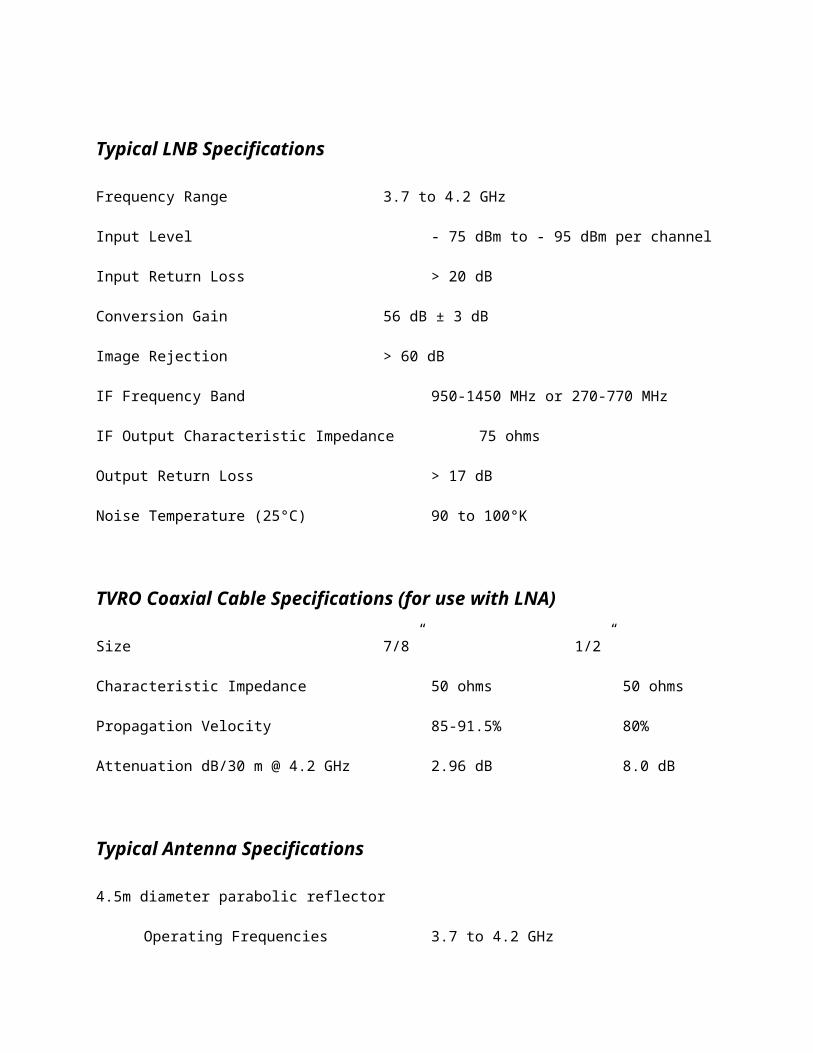
Typical LNB Specifications

Frequency Range 3.7 to 4.2 GHz

Input Level - 75 dBm to - 95 dBm per channel

Input Return Loss > 20 dB

Conversion Gain 56 dB ± 3 dB

Image Rejection > 60 dB

IF Frequency Band 950-1450 MHz or 270-770 MHz

IF Output Characteristic Impedance 75 ohms

Output Return Loss > 17 dB

Noise Temperature (25°C) 90 to 100°K

TVRO Coaxial Cable Specifications (for use with LNA)

Size 7/8” 1/2”

Characteristic Impedance 50 ohms 50 ohms

Propagation Velocity 85-91.5% 80%

Attenuation dB/30 m @ 4.2 GHz 2.96 dB 8.0 dB

Typical Antenna Specifications

4.5m diameter parabolic reflector

Operating Frequencies 3.7 to 4.2 GHz

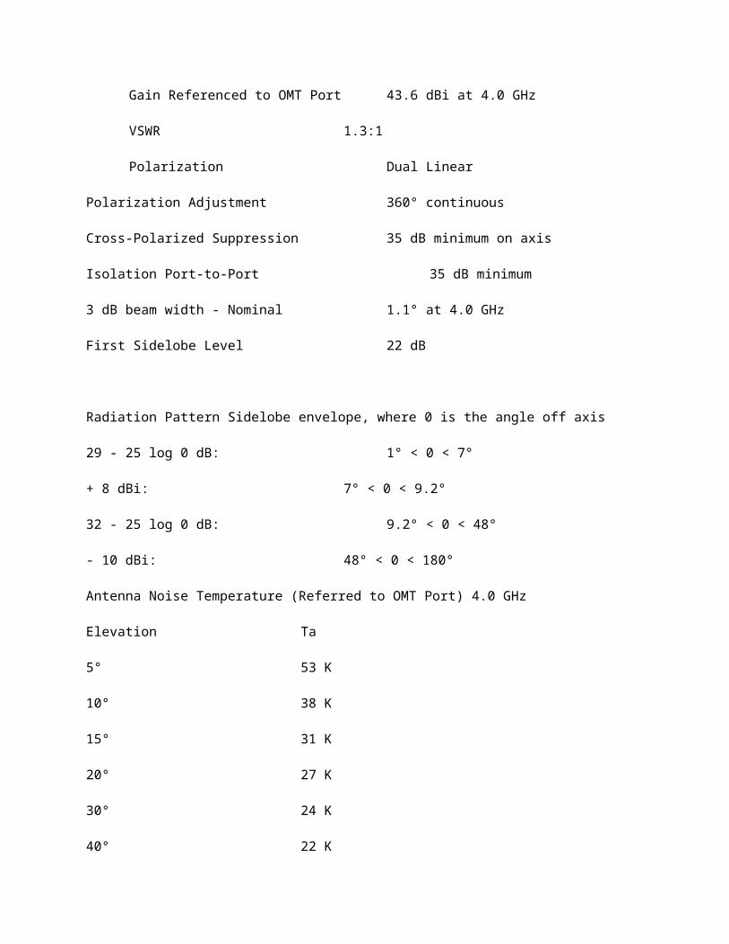
Gain Referenced to OMT Port 43.6 dBi at 4.0 GHz

VSWR 1.3:1

Polarization Dual Linear

Polarization Adjustment 360° continuous

Cross-Polarized Suppression 35 dB minimum on axis

Isolation Port-to-Port 35 dB minimum

3 dB beam width - Nominal 1.1° at 4.0 GHz

First Sidelobe Level 22 dB

Radiation Pattern Sidelobe envelope, where 0 is the angle off axis

29 - 25 log 0 dB: 1° < 0 < 7°

+ 8 dBi: 7° < 0 < 9.2°

32 - 25 log 0 dB: 9.2° < 0 < 48°

- 10 dBi: 48° < 0 < 180°

Antenna Noise Temperature (Referred to OMT Port) 4.0 GHz

Elevation Ta

5° 53 K

10° 38 K

15° 31 K

20° 27 K

30° 24 K

40° 22 K

50° 21 K

60° 21 K

B - Remote Hub Site / Headend

A remote hubsite or headend is a scaled-down version of the central headend. It does not

perform all of the functions of a central headend and may only process part of the cable

spectrum.

Remote Headend Functions:

• Receives satellite programming

• Receives off-air programming

• Demodulates FM signals from central headend

• Modulates programming onto cable channels

• Inserts channels into trunk system

• Inserts channels in return path of supertrunk to central headend.

Remote Hubsite Functions:

• Receives channels from AML

• Inserts channels into trunk.

C - AML Microwave

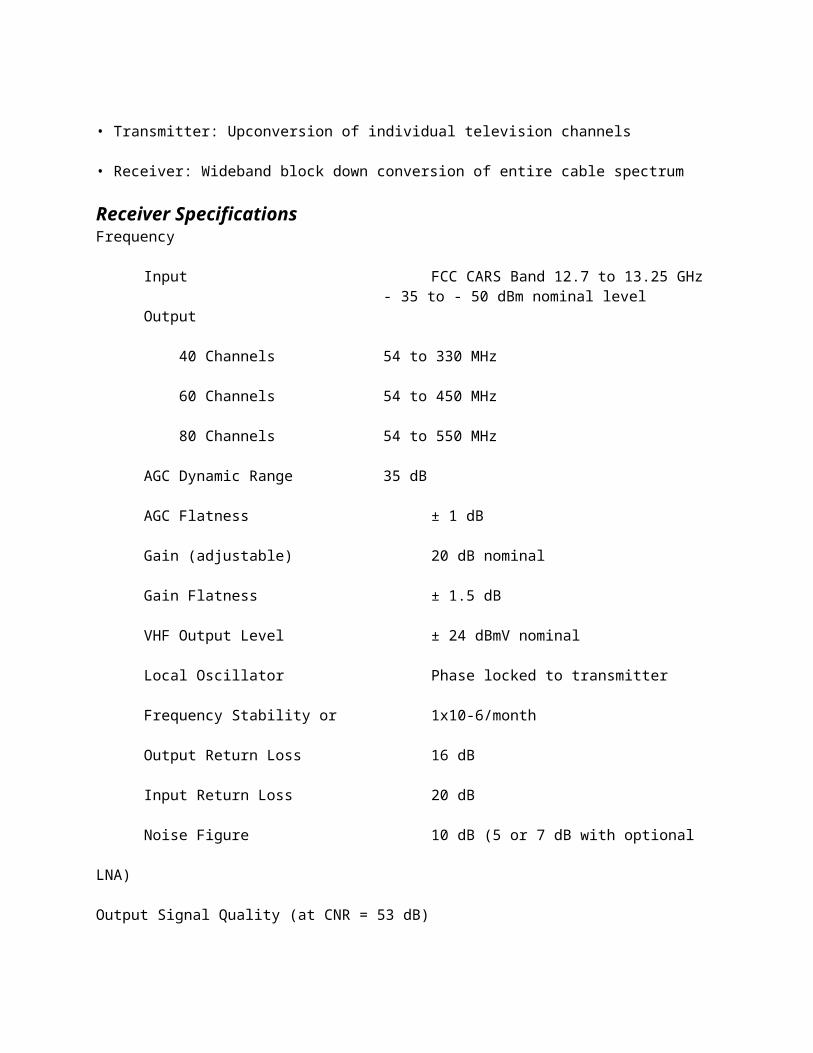
• Transmitter: Upconversion of individual television channels

• Receiver: Wideband block down conversion of entire cable spectrum

Receiver SpecificationsFrequency

Input FCC CARS Band 12.7 to 13.25 GHz- 35 to - 50 dBm nominal level

Output

40 Channels 54 to 330 MHz



AGC Dynamic Range 35 dB

AGC Flatness ± 1 dB

Gain (adjustable) 20 dB nominal

Gain Flatness ± 1.5 dB

VHF Output Level ± 24 dBmV nominal

Local Oscillator Phase locked to transmitter

Frequency Stability or 1x10-6/month

Output Return Loss 16 dB

Input Return Loss 20 dB

Noise Figure 10 dB (5 or 7 dB with optional LNA)

Output Signal Quality (at CNR = 53 dB)

40 channels 60 channels 80 channels

CTB

w/o LNA - 86 dB - 80 dB - 80 dB

with LNA - 78 dB - 72 dB - 72 dB

XMod

w/o LNA - 85 dB - 79 dB - 79 dB

with LNA - 77 dB - 71 dB - 71 dB

Hum Modulation 0.004 V rms

Transmitter Specifications

VHF Input Frequencies 54 to 550 MHz

Nominal Signal Input Level

Video Signals + 40 dBmV (-9 dBm)

Audio and FM Broadcast signals 17 dB below video

Output Frequencies CARS Band 12.7 to 13.25 GHz

Output Power (Single Channel)

High Power 5 W (+ 37 dBm)

Low Power 63 mW (+ 18 dBm)

Frequency Stability greater than ± 0.0005%

Modulation Type

High Power Single-Sideband Suppressed CarrierAmplitude Modulation (SSB-SC-AM)

Low Power Vestigial Sideband AmplitudeModulation (VSB-AM)

Input Return Loss 16 dB

Output Return Loss 16 dB

Group Delay ± 25 ns

Differential Gain 0.4 dB

Differential Phase 2°

D - FML Microwave• Single channel transmission 25 MHz per TV channel (12.5 MHz

optional)• Wideband receiver

System

Microwave frequency range 12.7 to 13.25 GHz

Frequency stability + 0.0005%

Modulation Frequency Modulation (FM)

Transmission Capacity 1 NTSC color video,plus 3 audio subcarriers

Equipment Specifications

Transmitter

Output Power 26 or + 37 dBm

Configuration IF heterodyne

Deviation (with CCIR 405-1 emphasis) ± 2.75 MHz peak

Input Baseband Levels/

Impedances/Return Loss/Connectors

Video 1 V p-p, 75 ohms, 26 dB, BNC

Audio - 10 dBm, 600 ohms, 26 dB,

terminal strip

Audio subcarriers frequency

offset from video carrier 4.5, 5.3 and 6.0 MHz

Audio Subcarrier Deviation ± 25 or ± 75 kHz peak

with 25 or 75 μs emphasis

Receiver

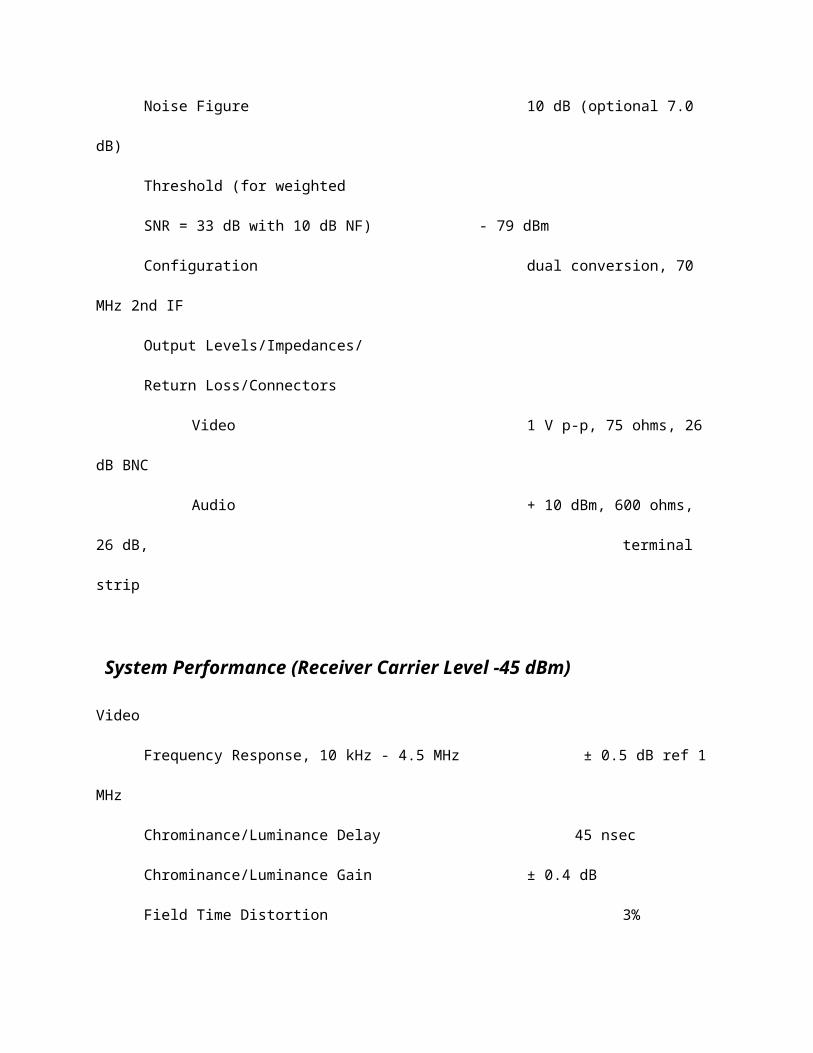
Noise Figure 10 dB (optional 7.0 dB)

Threshold (for weighted

SNR = 33 dB with 10 dB NF) - 79 dBm

Configuration dual conversion, 70 MHz 2nd IF

Output Levels/Impedances/

Return Loss/Connectors

Video 1 V p-p, 75 ohms, 26 dB BNC

Audio + 10 dBm, 600 ohms, 26 dB,

terminal strip

System Performance (Receiver Carrier Level -45 dBm)

Video

Frequency Response, 10 kHz - 4.5 MHz ± 0.5 dB ref 1 MHz

Chrominance/Luminance Delay 45 nsec

Chrominance/Luminance Gain ± 0.4 dB

Field Time Distortion 3%

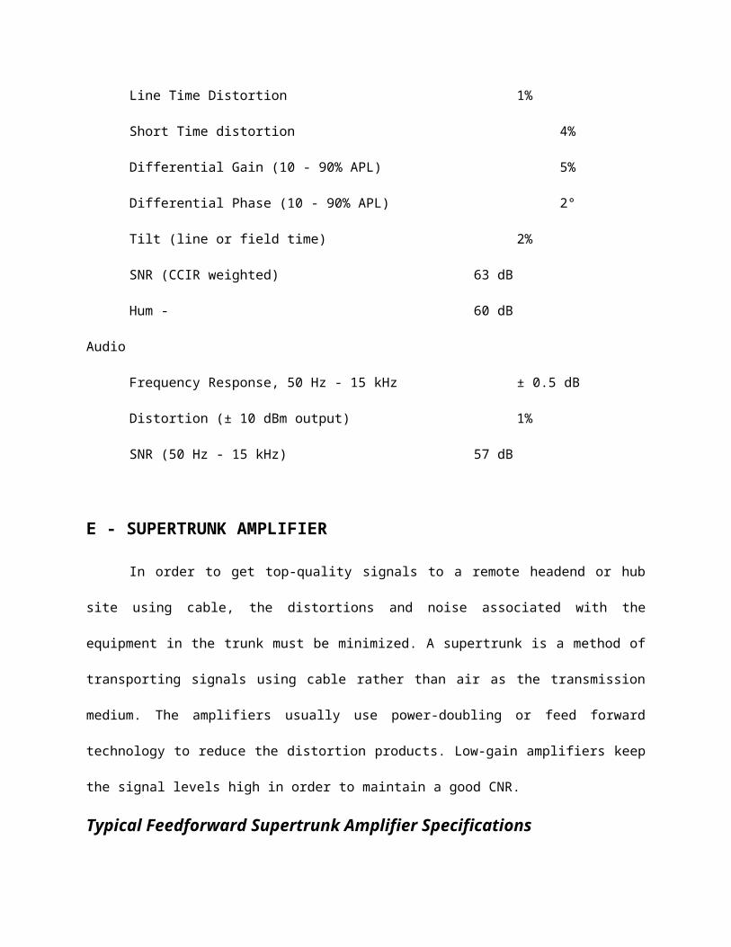
Line Time Distortion 1%

Short Time distortion 4%

Differential Gain (10 - 90% APL) 5%

Differential Phase (10 - 90% APL) 2°

Tilt (line or field time) 2%

SNR (CCIR weighted) 63 dB

Hum - 60 dB

Audio

Frequency Response, 50 Hz - 15 kHz ± 0.5 dB

Distortion (± 10 dBm output) 1%

SNR (50 Hz - 15 kHz) 57 dB

E - SUPERTRUNK AMPLIFIER

In order to get top-quality signals to a remote headend or hub site using cable, the

distortions and noise associated with the equipment in the trunk must be minimized. A

supertrunk is a method of transporting signals using cable rather than air as the transmission

medium. The amplifiers usually use power-doubling or feed forward technology to reduce the

distortion products. Low-gain amplifiers keep the signal levels high in order to maintain a good

CNR.

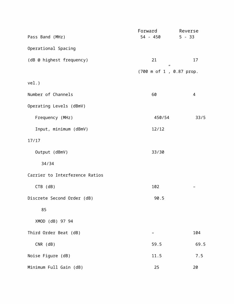
Typical Feedforward Supertrunk Amplifier Specifications

Forward ReversePass Band (MHz) 54 - 450 5 - 33

Operational Spacing

(dB @ highest frequency) 21 17

(700 m of 1”, 0.87 prop. vel.)

Number of Channels 60 4

Operating Levels (dBmV)

Frequency (MHz) 450/54 33/5

Input, minimum (dBmV) 12/12 17/17

Output (dBmV) 33/30 34/34

Carrier to Interference Ratios

CTB (dB) 102 –

Discrete Second Order (dB) 90.5 85

XMOD (dB) 97 94

Third Order Beat (dB) – 104

CNR (dB) 59.5 69.5

Noise Figure (dB) 11.5 7.5

Minimum Full Gain (dB) 25 20

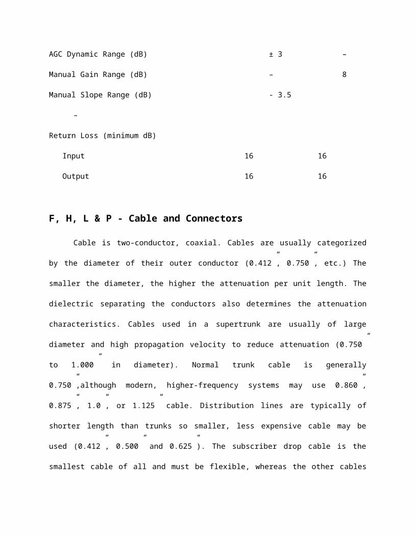
AGC Dynamic Range (dB) ± 3 –

Manual Gain Range (dB) – 8

Manual Slope Range (dB) - 3.5 –

Return Loss (minimum dB)

Input 16 16

Output 16 16

F, H, L & P - Cable and Connectors

Cable is two-conductor, coaxial. Cables are usually categorized by the diameter of their

outer conductor (0.412”, 0.750”, etc.) The smaller the diameter, the higher the attenuation per

unit length. The dielectric separating the conductors also determines the attenuation

characteristics. Cables used in a supertrunk are usually of large diameter and high propagation

velocity to reduce attenuation (0.750” to 1.000” in diameter). Normal trunk cable is generally

0.750”,although modern, higher-frequency systems may use 0.860”, 0.875”, 1.0”, or 1.125”

cable. Distribution lines are typically of shorter length than trunks so smaller, less expensive

cable may be used (0.412”, 0.500” and 0.625”). The subscriber drop cable is the smallest cable

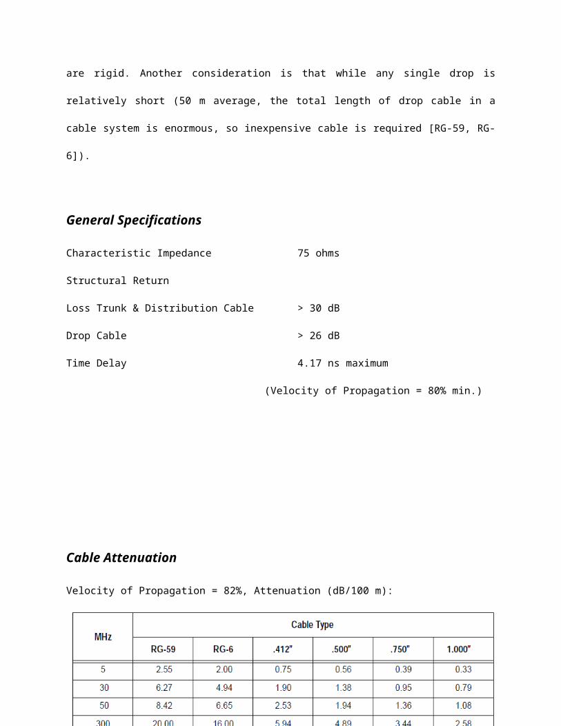
of all and must be flexible, whereas the other cables are rigid. Another consideration is that

while any single drop is relatively short (50 m average, the total length of drop cable in a cable

system is enormous, so inexpensive cable is required [RG-59, RG-6]).

General Specifications


Structural Return

Loss Trunk & Distribution Cable > 30 dB

Drop Cable > 26 dB

Time Delay 4.17 ns maximum

(Velocity of Propagation = 80% min.)

Cable Attenuation

Velocity of Propagation = 82%, Attenuation (dB/100 m):

Velocity of Propagation = 87%, Attenuation (dB/100m)

ConnectorsThere are two basic styles of connectors in use in the cable industry: feedthrough and

pin type. The feedthrough connector allows the center conductor of the cable to pass through

into the device to which the cable is connected. The pin type connector has a pin that clamps

the center connector in a captive seizure mechanism that then goes into the device. Pin

connectors allow the use of larger center conductors that may be too large for many passive

devices.

Typical Specifications

Attenuation NegligibleReturn Loss 30 dB minimum

G - TRUNK AMPLIFIERS

Amplifiers on the trunk radiating from a hub or headend that are not intended to be

supertrunks may have slightly reduced performance specifications. These may use push-pull or

power-doubling technology for systems with up to 60 channels. The station gain of these

trunk amplifiers may be higher than a supertrunk amplifier since the CNR or distortion is not

as critical. Systems with longer cascades and higher channel loading usually use feedforward

trunk amplifiers for improved performance.

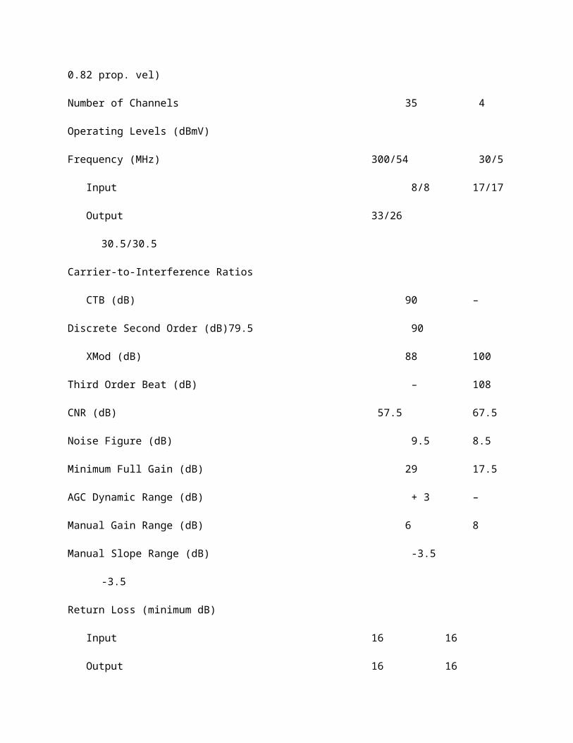
Typical Specifications for a Push-Pull Trunk Amplifier

Forward Reverse

Pass Band (MHz)54-300 5-40

Operational Spacing (dB)25 13.5

(700 m of 0.75,”

0.82 prop. vel)




Input 8/8 17/17

Output 33/26 30.5/30.5

Carrier-to-Interference Ratios

CTB (dB) 90 –

Discrete Second Order (dB)79.5 90

XMod (dB) 88 100


CNR (dB) 57.5 67.5


Minimum Full Gain (dB) 29 17.5

AGC Dynamic Range (dB) + 3 –

Manual Gain Range (dB) 6 8

Manual Slope Range (dB) -3.5 -3.5


Input 16 16

Output 16 16

Typical Specifications for a Power-Doubling Trunk Amplifier

Forward Reverse

Pass Band (MHz) 54-450 5-40

Operational Spacing (dB) 22 13

(500 m of 0.75”,

0.82 prop. vel)




Input 8/8 21/21

Output 30/24 34/34

Carrier-to-Interference Ratios

CTB (dB) 110 –

Discrete Second Order (dB) 88 88

XMod (dB) 96 104


CNR (dB) 58.5 70.5



AGC Dynamic Range (dB) ± 3 –


Manual Slope Range (dB) -10 -5


Input 16 16

Output 16 16

J - LINE SPLITTERS

Line splitters and/or directional couplers are used to split signals into two or three

different cables or devices.


K - FEEDER AMPLIFIERS

Feeder amplifiers or line extenders are used to amplify signals in the distribution areas.

Since there are many more feeder amplifiers in a cable system than trunk amplifiers, they must

be less expensive. The lower cost usually means lower performance specifications, which can

be tolerated because there are usually only two or three feeder amplifiers upstream of a

subscriber’s home.

Feeder amplifiers use either push-pull or power-doubling technology depending on how many

channels are on the system and what specification must be met at the subscriber’s terminal

device.

Typical Specification for Power Doubling Feeder Amplifier

Forward Reverse

Pass Band (MHz) 54-450 5-40

Operational Spacing (dB) 31 18

(300 m of 0.50,”

and multitaps)




Input 16/9 28/28

Output 47/40 46/46

Carrier to Interference Ratios

CTB (dB) 61 –

Discrete Second Order (dB) 66.5 68

XMod (dB) 61 76


CNR (dB) 65.5 80.5




Manual Slope Range (dB) -4 –


Input 16 16

Output 16 16

M - Multitaps

Multitaps allow for splitting the signals off the distribution cable for transmission along

the drop cable into the subscriber’s premises. Multitaps are actually a combination of directional

couplers and splitters designed to give the lowest insertion loss possible for the number of tap

legs and the tap loss desired. A common multitap spacing is 150 feet, although this varies

greatly with residence density.


Two-way:

Four-way:

Eight-way:

N - INDOOR SPLITTERS

Many subscriber premises are wired for more than one cable outlet. An indoor splitter

accomplishes this task at a low cost.


Q - CONVERTER

The set-top converter enables the subscriber to tune in the TV channels delivered by the

cable system that are outside the normal channel 2 to 13 VHF tuner of the television. This is

accomplished by down converting the selected channel to channel 2, 3, or 4. A choice of

channels is given so that interference from a local TV station can be avoided.


Input Bandwidth 54 to 450 MHz

Number of channels 60

Output channel 3 or 4

Channel Frequency Response ± 2 dB with6 MHz channel

Gain 0 to 9 dB

Noise Figure 13 dB

Return Loss

Input 7 dB minimum on tuned channel

Output 11 dB minimum

Isolation Input/Output 60 dB

Spurious Response

Input - 37 dBmV

Output - 57 dBmV in channel

Frequency Stability ± 250 kHz

Distortion at 15 dBmV;

60-channel load, flat input

Second Order - 57 dB

XMod - 57 dB

CTB - 57 dB

Input Level - 0 to + 20 dBmV

R - VIDEO CASSETTE RECORDER (VCR)

The VCR is the first device the cable signal encounters within the subscriber’s premises

that is beyond the control of the cable operator. A typical specification is difficult to obtain since

there are so many brands and models. A consideration worth noting, however, is that most

VCRs have a built-in splitter to enable the subscriber to record one channel while viewing

another. This splitter will reduce the signal levels by another 4 to 5 dB before reaching the

television.

S - TELEVISION

The television is the final device encountered by the cable signal. It is difficult to

characterize a typical TV since there are many manufacturers and models that have been

produced in the past 40 years or more. Like the VCR, this is another device that is beyond the

control of the cable system operator Government regulation provides for certain minimum

specifications at the input to the subscriber’s terminal device (usually a VCR or TV).

• TV carrier level input 0 to +14 dBmV

• Adjacent carrier levels within 3 dB

• Maximum difference between carrier levels within a 90-MHz band no greater than

8 dB

• Aural carrier level - 13 dB to -17 dB relative to video

• FM carrier levels -14 to +4 dBmV

• CNR minimum 36 dB

• Carrier-to-hum ratio 34 dB minimum

• Cross modulation ratio 48 dB minimum

• Carrier-to-beat ratio 58 dB minimum

• Carrier-to-composite beat ratio 53 dB minimum

• Echo Rating in any television channel 7% maximum

• Frequency response ± 1 dB within the 6 MHz television channel

• Chroma delay ± 150 nanoseconds.

ARCHITECTURAL DESIGN:

Optical nodes can cater 200 homes and an amplifier is needed every 300 meters.

INITIAL COST PER INSTALLATION

trunk amplifier every 300 meters:

11,571.25 x 4 = Php 46285

RG6 coaxial cable 100m

694.27 x 15 = Php 10414.05

outdoor taps

4633.60 x 10 = Php 46336

design for transmission systems

Documents

cable television

cable headend

drop cable

underground cable

coax cable

cable network

feeder cable

cable company