design, development and verification of a compensable
TRANSCRIPT

Design, Development and Verification of a
Compensable Workflow Modeling Language
By
Fazle Rabbi
Submitted in partial fulfillment of the
requirements for the degree of
Masters of Science in Computer Science
at
Saint Francis Xavier University
Antigonish, Nova Scotia
January 2011
c© Copyright by Fazle Rabbi, 2011

Saint Francis Xavier University
Department ofMathematics, Statistics and Computer Science
The undersigned hereby certify that they have read a thesis entitled “Design, Devel-opment and Verification of a Compensable Workflow Modeling Language”by Fazle Rabbi in partial fulfillment of the requirements for the degree of Masters ofScience.
Dated:
Supervisor:Dr. Wendy MacCaull
i

Dedicated to my parents
ii

Abstract
In recent years, Workflow Management Systems (WfMSs) have been studied and de-
veloped to provide automated support for defining and controlling various activities
associated with business processes. The automated support reduces costs and overall
execution time for business processes, by improving the robustness of the processes and
increasing productivity and quality of service. As business organizations continue to be-
come more dependent on computerized systems, the demand for reliability has increased.
Most WfMSs provide little or no verification facilities; this causes the resulting imple-
mentation of large and complex workflow models to be at risk of undesirable runtime
executions. Design validation, ensuring the correctness of the design at the earliest stage
possible, is a major challenge. Model checking is a promising and powerful approach to
automatic verification of systems, but model checking frequently suffers from the state
explosion problem and modeling with the input language of a model checker is time
consuming.
To address these issues, a compensable workflow modeling language called CWML is
designed and developed to provide both flexibility in the design, and also reliability in
the execution of a workflow system. In this research an automated translator is devel-
oped and studied which can translate a graphical workflow model and an abstract task
specification (written in Java) to the modeling language of the model checker DiVinE.
iii

To handle the state explosion problem a workflow reduction algorithm is developed and
integrated into the translator. A Service Oriented Architecture (SOA) based workflow
engine is designed and developed as part of the work. The effectiveness of the system
has been studied by developing a workflow based on the National Principles and Norms
of Practice of Canadian hospice palliative care. Finally, a sophisticated user friendly
browser is discussed with which one can see records in hierarchical fashion, travel to a
past record and can generate charts by selecing parameters. We show that the browser
can be used as a cause and effect analysis tool, which will aid the user for root cause
analysis and decision making.
iv

Acknowledgements
I am grateful to my supervisor Professor Dr. Wendy MacCaull for her help to solidify my
ideas in countless discussions. Her support and patience has been priceless during the
process of writing this thesis. The Centre for Logic and Information at StFX provided
a great environment to research with help from Keith Miller, Dr. Cristian Cocos, Dr.
Ji Ruan, Ahmed Mashiyat, Nazia Leyla, Maxwell Graham, Igor Vecei, Mary Heather
Jewers and many others. I owe special thanks to Dr. Hao Wang, who contributed
substantially to the ideas in this thesis and shared his knowledge of model checking and
high performance computing with me.
Additionally, I want to thank Dr. Man Lin and Dr. Laurence Yang for reading this
thesis and their feedback.
v

Contents
1 Introduction 1
2 Workflow systems overview 4
2.1 What is a workflow? . . . . . . . . . . . . . . . . . . . . . . . . . . . . . 4
2.2 Workflow modeling languages . . . . . . . . . . . . . . . . . . . . . . . . 5
2.3 Workflow enactment services . . . . . . . . . . . . . . . . . . . . . . . . . 8
3 Compensable transactions 11
3.1 The t-Calculus . . . . . . . . . . . . . . . . . . . . . . . . . . . . . . . . 15
3.2 The t-Calculus operators and their behavioral dependencies . . . . . . . 17
3.2.1 Sequential composition (;) . . . . . . . . . . . . . . . . . . . . . . 17
3.2.2 Parallel composition (||) . . . . . . . . . . . . . . . . . . . . . . . 18
3.2.3 Internal choice (⊓) . . . . . . . . . . . . . . . . . . . . . . . . . . 18
3.2.4 Speculative choice (⊗) . . . . . . . . . . . . . . . . . . . . . . . . 19
3.2.5 Alternative forwarding ( ) . . . . . . . . . . . . . . . . . . . . . 19
3.2.6 Backward handling (D) . . . . . . . . . . . . . . . . . . . . . . . . 20
3.2.7 Forward handling (⊲) . . . . . . . . . . . . . . . . . . . . . . . . 20
3.2.8 Programmable compensation (>) . . . . . . . . . . . . . . . . . . 21
vi

3.2.9 Associativity . . . . . . . . . . . . . . . . . . . . . . . . . . . . . 22
4 The compensable workflow modeling language 28
4.1 Compensable workflow nets . . . . . . . . . . . . . . . . . . . . . . . . . 28
4.2 The compensable workflow modeling language and its Petri net represen-
tation . . . . . . . . . . . . . . . . . . . . . . . . . . . . . . . . . . . . . 34
4.3 Analysis . . . . . . . . . . . . . . . . . . . . . . . . . . . . . . . . . . . . 44
5 Model checking and automated translation 48
5.1 Model checking . . . . . . . . . . . . . . . . . . . . . . . . . . . . . . . . 48
5.1.1 The DiVinE model checker and its modeling language . . . . . . . 50
5.2 Workflow translation to a model checker . . . . . . . . . . . . . . . . . . 52
5.2.1 Petri net to DVE translation . . . . . . . . . . . . . . . . . . . . . 55
5.2.2 Proof of correctness . . . . . . . . . . . . . . . . . . . . . . . . . . 59
6 Workflow model reduction 64
6.1 Related work . . . . . . . . . . . . . . . . . . . . . . . . . . . . . . . . . 64
6.1.1 Partial order reduction . . . . . . . . . . . . . . . . . . . . . . . . 64
6.1.2 Other work . . . . . . . . . . . . . . . . . . . . . . . . . . . . . . 70
6.2 Workflow model reduction . . . . . . . . . . . . . . . . . . . . . . . . . . 70
6.3 Proof of stuttering equivalence . . . . . . . . . . . . . . . . . . . . . . . . 75
6.4 Effectiveness . . . . . . . . . . . . . . . . . . . . . . . . . . . . . . . . . . 87
7 Tool overview 90
7.1 NOVA workflow . . . . . . . . . . . . . . . . . . . . . . . . . . . . . . . . 91
7.1.1 The NOVA editor . . . . . . . . . . . . . . . . . . . . . . . . . . . 91
vii

7.1.2 The NOVA engine . . . . . . . . . . . . . . . . . . . . . . . . . . 93
7.1.3 The NOVA translator . . . . . . . . . . . . . . . . . . . . . . . . 96
7.1.4 The NOVA browser . . . . . . . . . . . . . . . . . . . . . . . . . . 98
8 Case study 104
8.1 Hospice palliative care . . . . . . . . . . . . . . . . . . . . . . . . . . . . 104
8.2 Verification of the palliative care process . . . . . . . . . . . . . . . . . . 113
9 Conclusion and future work 120
Bibliography 123
viii

List of Figures
2.1 Workflow system characteristics . . . . . . . . . . . . . . . . . . . . . . . 5
2.2 An example of a Petri net . . . . . . . . . . . . . . . . . . . . . . . . . . 7
2.3 Workflow reference model - components & interfaces . . . . . . . . . . . 9
3.1 State transition diagram of a compensable transaction . . . . . . . . . . . 12
4.1 Petri net representation of an atomic uncompensable task . . . . . . . . . 29
4.2 Petri net representation of an atomic compensable task . . . . . . . . . . 30
4.3 Graphical representation of CWML . . . . . . . . . . . . . . . . . . . . . 34
4.4 n-fold split and join tasks . . . . . . . . . . . . . . . . . . . . . . . . . . 36
4.5 Petri net representation of and composition . . . . . . . . . . . . . . . . 36
4.6 Petri net representation of xor composition . . . . . . . . . . . . . . . . . 37
4.7 Petri net representation of or composition . . . . . . . . . . . . . . . . . 37
4.8 Petri net representation of sequential composition . . . . . . . . . . . . . 38
4.9 Petri net representation of internal choice composition . . . . . . . . . . 39
4.10 Petri net representation of alternative forward composition . . . . . . . . 40
4.11 Petri net representation of parallel composition . . . . . . . . . . . . . . 41
4.12 Petri net representation of speculative choice composition . . . . . . . . . 43
4.13 CWF-net with one atomic task . . . . . . . . . . . . . . . . . . . . . . . 45
ix

4.14 CWF-net with one compensable task . . . . . . . . . . . . . . . . . . . . 46
4.15 CWF-net with more compensable tasks . . . . . . . . . . . . . . . . . . . 47
5.1 A Petri net . . . . . . . . . . . . . . . . . . . . . . . . . . . . . . . . . . 56
6.1 Execution of independent transitions . . . . . . . . . . . . . . . . . . . . 67
6.2 If AP’ = {p} then α is invisible . . . . . . . . . . . . . . . . . . . . . . . 67
6.3 Two stuttering equivalent paths . . . . . . . . . . . . . . . . . . . . . . . 68
6.4 Example of a task syntax tree . . . . . . . . . . . . . . . . . . . . . . . . 71
6.5 The workflow Mex . . . . . . . . . . . . . . . . . . . . . . . . . . . . . . . 74
6.6 The task syntax tree for Mex . . . . . . . . . . . . . . . . . . . . . . . . . 75
6.7 The reduced workflow M ′ex . . . . . . . . . . . . . . . . . . . . . . . . . . 76
6.8 Forming a syntax tree of size k + 1 from one of size k . . . . . . . . . . . 79
6.9 Sequential composition (•) of uncompensable atomic tasks . . . . . . . . 80
6.10 Reduced syntax tree τ ′k+1 . . . . . . . . . . . . . . . . . . . . . . . . . . . 81
6.11 Reduced syntax tree τ ′k+1 . . . . . . . . . . . . . . . . . . . . . . . . . . . 83
6.12 Workflow with and composition . . . . . . . . . . . . . . . . . . . . . . . 88
7.1 SOA based architecture of NOVA workflow . . . . . . . . . . . . . . . . . 92
7.2 NOVA editor in eclipse IDE . . . . . . . . . . . . . . . . . . . . . . . . . 93
7.3 NOVA engine guides the service flow . . . . . . . . . . . . . . . . . . . . 94
7.4 An example of a service class extension . . . . . . . . . . . . . . . . . . . 94
7.5 Syntax for assigning non-deterministic data . . . . . . . . . . . . . . . . 97
7.6 DVE code for non-deterministic data . . . . . . . . . . . . . . . . . . . . 98
7.7 Hierarchical data representation in the NOVA browser . . . . . . . . . . 100
7.8 Example of a chart view . . . . . . . . . . . . . . . . . . . . . . . . . . . 103
x

8.1 Overview of CHPCA model . . . . . . . . . . . . . . . . . . . . . . . . . 105
8.2 Palliative care workflow: Overall . . . . . . . . . . . . . . . . . . . . . . 107
8.3 GASHA Form: Adult pain meter . . . . . . . . . . . . . . . . . . . . . . 107
8.4 Registration . . . . . . . . . . . . . . . . . . . . . . . . . . . . . . . . . . 111
8.5 Palliative care workflow: Intake . . . . . . . . . . . . . . . . . . . . . . . 111
8.6 Palliative care workflow: Regular Assessment . . . . . . . . . . . . . . . . 112
8.7 Palliative care workflow: Team Building . . . . . . . . . . . . . . . . . . 114
xi

Chapter 1
Introduction
Workflow management systems (WfMS) provide an important technology for the de-
sign of computer systems which can improve process, communication and information
system development in dynamic and distributed organizations. Current Workflow Man-
agement Systems (WfMSs) facilitate the enactment of workflows with some degree of
fault-tolerance, e.g., exception handling, but often provide limited formal verification
capacity which is especially important in safety critical systems. For example, YAWL
(Yet Another Workflow Language) [40] can verify the soundness property of workflow
nets (a sub class of Petri nets) which guarantees the absence of live-locks, deadlocks,
and other anomalies without domain knowledge [44]. There are several other graphical
tools for modeling workflow systems (e.g., Petri nets [33], ADEPT2 [37]) but they do not
provide formal verification. WSEngineer [8] and BPEL2PN [6] have recently been devel-
oped for the verification of BPEL (Business Process Execution Language) [20], but the
built-in support for compensation in BPEL does not provide rich semantics of compen-
sation compared to the t-Calculus [29]. Moreover, these tools lack advanced workflow
reduction techniques.
1

In this thesis we present our new graphical workflow modeling language, the Com-
pensable Workflow Modeling Language (CWML), with which one can model a workflow
with compensation. The foundation of the CWML is based on Petri nets [33]. We incor-
porated rich semantics of compensation into the CWML with the help of t-Calculus [29]
operators. We developed a tool named NOVA Workflow [7] to design, develop, verify
and analyze compensable workflows. We detail our algorithm to translate a CWML
workflow model to DVE, the input language of a model checker DiVinE [1], and give
its proof of correctness. DiVinE is a parallel distributed model checker which can verify
large systems. In addition to that we give our algorithm for a workflow reduction tech-
nique which pre-processes a workflow model and reduces the model in such a way that
the reduced workflow model is stuttering equivalent to the original model with respect
to an LTL property. The pre-processing significantly reduces the size of the state space
while verifying the workflow in the DiVinE model checker. The tool was used to model
and verify properties of the national model of CHPCA [16] which shows its applicability.
In chapter 2, we give a brief description of existing workflow management systems along
with their modeling languages. We are especially interested in graphical workflow mod-
eling languages. Chapter 3 provides a detailed description of compensable transactions
and t-Calculus operators. The internal constraints and behavioral dependencies of com-
pensable transactions described in this chapter help clarify the concept of compensable
transaction. In chapter 4 we define a new Compensable Workflow Modeling Language
(CWML) and present the graphical representation of compensable tasks. Compensable
tasks are based on the idea of compensable transactions and t-Calculus operators. We
use Petri nets to describe the semantics of compensable tasks. In chapter 5 we give an
algorithm to translate a CWML workflow to the model checker DiVinE. The proof of
2
correctness of the algorithm is shown in this chapter. In order to verify a large work-
flow by a model checker, we provide a workflow reduction algorithm in chapter 6. The
proof of stuttering equivalence of the original and reduced model and its effectiveness
are shown in this chapter. Chapter 7 provides a tool overview of the workflow suite,
called NOVA Workflow, that we developed. NOVA Workflow consists of four compo-
nents, i) the NOVA Editor, ii) the NOVA Translator, iii) the NOVA Engine and iv) the
NOVA Browser. This chapter gives a description of each component. With this tool we
can input a workflow modeled with CWML using the graphical editor, and an LTL−X
formula. The reduction, translation and model checking then all proceed automatically
giving either a counter-model if the specification fails, or a statement that the model sat-
isfies the specification. We provide a case study in chapter 8. A workflow was developed
for a community based palliative care program using NOVA Workflow and a number of
properties were verified. Chapter 9 summarizes our specific contributions and discusses
some of our future work.
3

Chapter 2
Workflow systems overview
2.1 What is a workflow?
Workflow is concerned with the automation of a process, in whole or part, during which
documents, information or tasks are passed from one participant to another for action
(activities), according to a set of procedural rules. A participant may be a person or
an automated process (computer system). Workflow can be a sequential progression of
work activities or a complex set of processes each taking place concurrently, eventually
impacting each other according to a set of rules, routes, and roles. A Workflow Man-
agement System is a system that completely defines, manages and executes “workflows”
through the execution of software whose order of execution is driven by a computer
representation of the workflow logic. At the highest level, all WfM systems may be
characterised as providing support in three functional areas [19]:
• Build-time functions, concerned with defining, and possibly modelling, the work-
flow process and its constituent activities;
4

• Run-time control functions concerned with managing the workflow processes in an
operational environment and sequencing the various activities to be handled as
part of each process;
• Run-time interactions with human users and IT application tools for processing
the various activity steps.
Fig. 2.1 illustrates the basic characteristics of WfM systems and the relationships
between these main functions.
Figure 2.1: Workflow system characteristics
2.2 Workflow modeling languages
A number of graphical process-modeling languages are available to define the detailed
routing and processing requirements of a typical workflow [46]. For the purpose of our
5

work we are interested in languages with a sound mathematical foundation such as Petri
nets and Workflow nets.
Petri nets
Historically speaking, Petri nets originate from the early work of Carl Adam Petri [33].
Since then the use and study of Petri nets have increased considerably. For a review of
the history of Petri nets and an extensive bibliography the reader is referred to [32].
The classical Petri net is a directed bipartite graph with two node types called places
and transitions. The nodes are connected via directed arcs. Connections between two
nodes of the same type are not allowed. Places are usually represented by circles and
transitions are usually represented by rectangles. The mathematical definition of a Petri
net is given below:
Definition 2.1. A Petri net is a 5-tuple, PN = (P, T, F,W,M0) where:
• P = {p1, p2, ...., pm} is a finite set of places,
• T = {t1, t2, ...., tn} is a finite set of transitions,
• F ⊆ (P × T ) ∪ (T × P ) is a set of arcs (flow relation),
• W: F → {1,2,3,...} is a weight function,
• M0: P → {0,1,2,3,...} is the initial marking,
• P ∩ T = φ and P ∪ T 6= φ.
A marking of a Petri net is a multiset of its places, i.e., a mapping M : P → N. We
say the marking assigns to each place a number of tokens.
6

A 4-tuple N = (P, T, F,W ) is called a Petri net structure (no specific initial marking)
Places may contain tokens and the distribution of tokens among the places of a Petri
net determine its state (or marking). Fig. 2.2 shows an example of a Petri net where
P1, P2, P3, P4 are places, t1 and t2 are transitions and the dots represent the tokens of
places P1, P3 and P4.
Figure 2.2: An example of a Petri net
Workflow nets
Workflow nets, based on the characteristics of Petri nets, is a powerful and flexible
language to model control flows [41].
Definition 2.2. A Petri net structure N = (P, T, F,W ) is called a workflow net (WF-
net) if and only if:
• N has one source place i, called the initial place.
• N has one sink place f, called the final place.
• for every node n ∈ P ∪ T , there exists a path from i to n and a path from n to f.
Places in the set P correspond to conditions, transitions in the set T correspond
to tasks. Tokens in a WF-net represent the workflow state of a single instance of a
7

workflow execution. One of the advantages of using Petri nets for workflow modeling is
the availability of many Petri net based analysis techniques [42].
Other modeling languages
The Business Process Modeling Language (BPML) [9] is an XML based markup language
designed to model business processes deployed over the Internet. The BPML specifi-
cation provides an abstract model and XML syntax for expressing executable business
processes and supporting entities. BPML specifies transactions, data flow, messages
and scheduled events, business rules, security roles, and exceptions. It supports both
synchronous and asynchronous distributed transactions.
2.3 Workflow enactment services
A workflow enactment service provides the run-time environment in which process in-
stantiation and activation occurs. Fig. 2.3 illustrates the major components and inter-
faces within the workflow reference model [19].
Definition 2.3. Workflow Enactment Service is a software service that may consist of
one or more workflow engines in order to create, manage and execute workflow instances.
Applications may interface with this service via a workflow application programming
interface (API).
Definition 2.4. A Workflow Engine is a software service or “engine” that provides the
run time execution environment for a workflow instance.
8

Figure 2.3: Workflow reference model - components & interfaces
Interaction with external resources accessible to the particular enactment service
occurs via one of two interfaces:
• The client application interface, through which a workflow engine interacts with a
worklist handler, responsible for organising work on behalf of a user resource. It
is the responsibility of the worklist handler to select and progress individual work
items from the work list. Activation of application tools may be under the control
of the worklist handler or the end-user.
• The invoked application interface, which enables the workflow engine to directly
activate a specific tool to undertake a particular activity. This would typically be
a server-based application with no user interface; where a particular activity uses a
tool which requires end-user interaction. The server based application would nor-
mally be invoked via the worklist interface to provide more flexibility for user task
9

scheduling. By using a standard interface for tool invocation, future application
tools may be workflow enabled in a standardised manner.
10
Chapter 3
Compensable transactions
A traditional system which consists of ACID (Atomic, Consistent, Isolated, Durable)
transactions cannot handle long lived transactions as it has only a flow in one direction.
A long lived transaction system is composed of sub-transactions and therefore has a
greater chance of partial effects remaining in the system in the presence of some failure.
These partial effects make traditional rollback operations infeasible or undesirable. A
transaction is called a compensable transaction, when its effects can be semantically
removed by some compensating actions [26]. A compensable transaction has two flows:
a forward flow and a compensation flow. The forward flow executes the normal business
logic according to the system requirements, while the compensation flow removes all
partial effects by acting as a backward recovery mechanism in the presence of some
failure.
The concept of a compensable transaction was first proposed by Garcia-Molina and
Salem [17], who called this type of long-lived transactions, a saga. A saga can be
broken into a collection of sub-transactions that can be interleaved in some way with
other sub-transactions. This allows sub-transactions to commit prior to the completion
11

of the whole saga. Here commit refers to the idea of making a set of tentative changes
permanent. To make sure that the system is consistent while performing any transaction,
it needs to lock system resources (e.g., database tables, files, etc.). If a system resource
is locked for a long time, it might increase the chance of deadlock. Dividing a long-lived
transactions into sub-transactions (possibly short-lived transactions) releases resources
earlier and reduces the possiblity of deadlock. If the system needs to rollback in case of
some failure, each sub-transaction executes an associated compensation to semantically
undo the committed effects of its own committed transaction.
A compensable transaction may be described by its external state. In [27] we find
there is a finite set of eight independent states, called transactional states, which can
be used to describe the external state of a transaction at any time. These transactional
states are idle (idl), active (act), aborted (abt), failed (fal), successful (suc), undoing
(und), compensated (cmp), and half-compensated (hap), where idl, act, etc. are the
abbreviated forms. Among the eight states, suc, abt, fal, cmp, hap are the terminal
states. The transition relations among the states are illustrated in Fig. 3.1 [27].
Figure 3.1: State transition diagram of a compensable transaction
∑
is used to represent the finite set of transactional states. ∆ is used to represent
the set of terminal states, which is a subset of∑
, i.e.,
∑
= { idl, act, suc, abt, fal, und, cmp, hap }
∆ = { suc, abt, fal, cmp, hap }
12

∆ ⊆∑
.
Before activation, a compensable transaction is in the idle state. Once activated, the
transaction eventually moves to one of five terminal states. A successful transaction has
the option of moving to the undoing state. If the transaction can successfully undo all its
partial effects it goes to the compensated state, otherwise it goes to the half-compensated
state.
An ordered pair consisting of a compensable transaction and its state is called a
transactional action (called an action in [27]). Transactional actions are used to describe
the behavioural dependencies of compensable transactions. In [27], five binary relations
were proposed to define the constraints applied to transactional actions on compensable
transactions. Informally the relations are described in Table 3.1, where both a and b
are transactional actions:
1. a < b only a can fire b
2. a ≺ b b can be fired by a
3. a ≪ b a is the precondition of b
4. a ↔ b a and b both occur or both not
5. a = b the occurance of one transactional action inhibits the other
Table 3.1: Behavioural dependencies of compensable transactions
The first three relations specify the order of execution, whereas the last two do not.
a < b indicates that a must precede b when the two transactional actions both occur,
and that either the two transactional actions both occur or neither occurs. a ↔ b
indicates that either both transactional actions occur or neither occurs but a ↔ b does
13

not impose any temporal constraint on transactional actions. a ≺ b tells us that if a
occurs b must follow, but b can occur without a previous occurance of a. a ≪ b tells
us that whenever b occurs, a must occur earlier. However, the occurrence of a does not
guarantee a following occurrence of b. Finally, a = b denotes that the two transactional
actions must be mutially exclusive. These relations can be mathematically expressed by
the following formulae, where s is a sequence of transactional actions and s [i ] denotes
the ith element in the sequence:
(R1) s satisfies a < b iff ∃i, j such that (i<j ∧ s[i] = a ∧ s[j] = b ) ∨ ∀i.(s[i] 6= a ∧ s[i] 6= b)
(R2) s satisfies a ≺ b iff ∀i (s[i] = a⇒ ∃j. (j > i ∧ s[j] = b))
(R3) s satisfies a ≪ b iff ∀i (s[i] = b⇒ ∃j. (j<i ∧ s[j] = a))
(R4) s satisfies a ↔ b iff ∃i, j such that(s[i] = a ∧ s[j] = b) ∨ ∀i.(s[i] 6= a ∧s[i] 6= b)
(R5) s satisfies a = b iff ∃i such that (s[i] = a⇒ ∀j.s[j] 6= b)
The relations <, ≺, ≪ are anti-symmetric and transitive. The relation ↔ is reflexive, sym-
metric and transitive, while = is irreflexive, symmetric and intransitive. In addition, these
relations exhibit the following useful properties [27]:
• Law 1. If a < b and a ↔ b then b ↔ c
• Law 2. If a < b and b ↔ c then a ↔ c
• Law 3. If a < b and b ◦ c (◦ ∈ {≺,≪}) then a ◦ c
• Law 4. If a ◦ b (◦ ∈ {≺,≪}) and b < c then a ◦ c
• Law 5. If a ◦ b (◦ ∈ {<,≺,↔}) and b = c then a = c
• Law 6. If a ◦ b (◦ ∈ {<,≪,↔}) and a = c then b = c
14

For an arbitrary compensable transaction T , all the transactional actions occurring during
its execution must satisfy some constraints which are shown in Table 3.2.
(T,idl) ≪ (T,act) (T,act) ≪ (T,suc) (T,act) ≪ (T,abt) (T,act) ≪ (T,fal)
(T,suc) = (T,abt) (T,suc) = (T,fal) (T,abt) = (T,fal) (T,cmp) = (T,hap)
(T,suc) ≪ (T,und) (T,und) ≪ (T,cmp) (T,und) ≪ (T,hap)
Table 3.2: Intra-constraints of a compensable transaction
The transactional language t-Calculus was introduced by Li et al [29] to model business
flow in terms of compensable transactions. t-Calculus provides a framework to combine com-
pensable transactions allowing one to setup a long running business transaction which has
compensation as its main error recovery technique.
3.1 The t-Calculus
The transactional language t-Calculus is intended to describe the behavior of top-level transac-
tions [26]. Transactions are modeled in terms of atomic activities and a number of operators are
introduced to support compensable transactions. An atomic activity is an activity for which
no errors can take place during the execution. We use an infinite set of names to represent
atomic activities ranged over by A,B, .... . Moreover, we consider two other special activities:
the empty activity 0 always completes but has no effect; the error activity ♦ always leads to
a fail state.
A compensable transaction consists of two parts: a forward flow and a compensation flow.
In case of failure, compensation will be activated to compensate its forward flow. The basic
way to construct a compensable transaction is through a transactional pair A÷B, where A is
15
the forward flow and B is its compensation. The compensation B is responsible for undoing
the effect of A. Especially, A÷ 0 denotes that the forward flow A is associated with an empty
compensation. In other words, the effect made by A does not need to be removed when error
occurs. Besides, not every activity can be semantically undone, so sometimes the application
designer cannot find a suitable compensation. In this case, we use A ÷ ♦ to denote that the
forward flow A is associated with an unacceptable compensation which always encounters a
failure.
There are three variations for basic transactions. Skip stands for a successfully completed
transaction without anything really done. Abort means a certain error has taken place and
all composed compensations should be activated to recover from this failure. Fail indicates
an error too; however, it has no mechanism to enable compensations and causes an exception
instead.
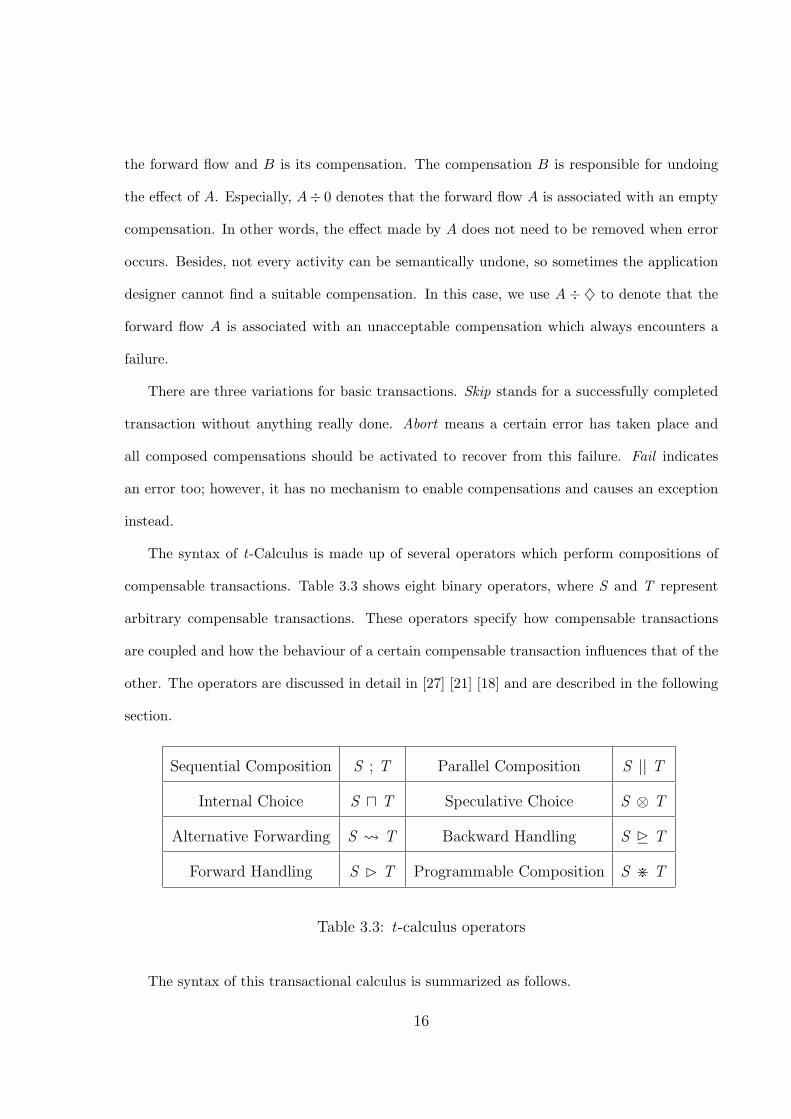
The syntax of t-Calculus is made up of several operators which perform compositions of
compensable transactions. Table 3.3 shows eight binary operators, where S and T represent
arbitrary compensable transactions. These operators specify how compensable transactions
are coupled and how the behaviour of a certain compensable transaction influences that of the
other. The operators are discussed in detail in [27] [21] [18] and are described in the following
section.
Sequential Composition S ; T Parallel Composition S || T
Internal Choice S ⊓ T Speculative Choice S ⊗ T
Alternative Forwarding S T Backward Handling S D T
Forward Handling S ⊲ T Programmable Composition S > T
Table 3.3: t-calculus operators
The syntax of this transactional calculus is summarized as follows.
16

BT ::= A÷B | A÷ 0 | A÷♦ | Skip | Abort | Fail
S, T ::= BT | S;T | S||T | S ⊓ T | S ⊗ T | S T | S D T | S ⊲ T | S > T
Where BT denotes a basic transaction, S,T denote arbitrary transaction.
3.2 The t-Calculus operators and their behavioral
dependencies
t-Calculus operators can be semantically defined by behavioural dependencies, expressed us-
ing the five relations <, ≺, ≪, ↔, = (see Table 3.1). The functionality and behavioural
dependencies of these operators are discussed in this section.
3.2.1 Sequential composition (;)
The sequential composition S ; T, denotes a sequential ordering of transactions. In the compos-
ite transaction S;T the transaction S would begin execution, and the transaction T starts its
execution once S has completed successfully. However, whenever T is aborted or compensated,
the completed transaction S would be compensated so as to remove all the partial effects. The
above description is reflected in the following behavioral dependencies [27]:
(S,suc) < (T,act) ;
(T,abt) ≺ (S,und) ;
(T,cmp) ≺ (S,und) .
Additional behavioural dependencies can be derived from the behavioural dependencies of
sequential composition using the laws governing the internal constraints (found in Table 3.3)
of compensable transactions [27]. Some of them are listed below:
(S,suc) ≪ (T,α), α ∈ ∆ ;
(S,α) = (T,β), α ∈ {abt, fal} and β 6= idl ;
17

(S,α) = (T,β), α ∈ {cmp, hap} and β ∈ {fal, hap} .
3.2.2 Parallel composition (||)
The parallel composition, S || T, describes the composition of two compensable transactions
running in parallel. Their compensations are activated concurrently when semantic rollback is
needed. If one transaction aborts or fails, the other transaction tries to abort. This is achieved
by an internal mechanism called forceful abort, which forcefully halts a transaction and leaves
no partial effects. In other words, the two transactions reach the successful state or reach
either the abort or fail state. Below is a listing of the behavioural dependencies of parallel
composition [27]:
(S,act) ↔ (T,act) ;
(S,und) ↔ (T,und) ;
(S,suc) ↔ (T,suc) .
Other dependencies can be deduced. For example:
(S,α) = (T,β) α ∈ {abt, fal}, β ∈ {suc, cmp, hap} ;
(T,α) = (S,β) α ∈ {abt, fal}, β ∈ {suc, cmp, hap} .
3.2.3 Internal choice (⊓)
The internal choice composition, S ⊓ T, denotes the selection and execution of one, and only
one, of the composed sub-transactions. Therefore, either S or T must be activated but not
both. The transaction is selected on the basis of some internal data of the system. There is
one basic behavioural dependency for ⊓ [27]:
(S,act) = (T,act) .
An additional behavioural dependency can be derived:
(S,α) = (T,β), {α, β} ⊆ ∆ .
18

3.2.4 Speculative choice (⊗)
The speculative choice composition, S ⊗ T, provides a way for designers to permit two or
more threads to finish one task. If one thread is aborted, the other thread is still active
trying to achieve the same task. In S ⊗ T, S and T are two sub-transactions with similar
goals. The two sub-transactions have the same priority and they are arranged to be executed
concurrently. The choice is delayed until one sub-transaction has succeeded. That is, only
one sub-transaction will be selected to achieve its business goal. When one sub-transaction
terminates successfully, the other one cannot succeed but aborts either internally or forcibly.
Also, as with parallel composition, if either sub-transaction results in a failed state then the
entire speculatively composed transaction will result in the failed state. This is due to the
unavoidable remaining partial effect of that failed sub-transaction. The related behavioral
dependencies are formalized below [27]:
(S,act) ↔ (T,act) ;
(S,suc) = (T,suc) ;
(S,suc) = (T,fal) ;
(T,suc) = (S,fal) .
The above dependencies imply that only one sub-transaction can be compensated if compen-
sation is needed, i.e.:
(S,α) = (T,β), {α, β} ⊆ {cmp, hap} .
3.2.5 Alternative forwarding ( )
As with speculative choice, the alternative forwarding composition, S T , provides two
functionally equivalent sub-transactions to achieve one business goal. The difference is that
with , these two sub-transactions have distinct priorities. In addition, the one with the
higher priority is executed first and the other is activated only when the first one has been
19

aborted. Thus, in S T, S runs first and T is the backup of S. The related dependency is
given below [27]:
(S,abt) < (T,act) .
and the following dependencies can be derived:
(S,abt) ≪ (T,α) α ∈ ∆ ;
(S,α) = (T,β) α ∈ ∆− {abt}, β ∈ ∆ .
3.2.6 Backward handling (D)
The backward handling composition, S D T, is one of two error handling operators which
exists in the t-Calculus. Backward handling focuses on handling any partial effects or data
inconsistencies resulting from an error. If an error occurs in S then T will attempt to remove
any partial effects and if this is completed successfully then the compensating flow of the system
is triggered. This behaviour is represented by the following basic behavioural dependency [27]:
(S,fal) < (T,act) .
From this dependency the following behavioural dependencies can be derived:
(S,fal) ≪ (T,α), α ∈ ∆ ;
(S,α) = (T,β), α ∈ ∆− {fal}, β ∈ ∆ .
3.2.7 Forward handling (⊲)
The forward handling composition, S ⊲ T, is the second of the two error handling composition
operators of the t-Calculus. Forward handling serves the same purpose as backward handling,
in that its purpose is to remove any remaining partial effects from S if an error occurs in S.
The main difference between the two operators is that the forward handling operator does not
start the compensating flow once an error is detected. Instead, the forward handling operator
continues with the forward flow of the system, in an effort to complete the goal of the system.
20

The forward handling operator has the following basic behavioural dependency [27]:
(S,fal) < (T,act) .
These following behaviour dependencies can be derived from the basic behavioural dependency
listed above:
(S,fal) ≪ (T,α), α ∈ ∆ ;
(S,α) = (T,β), α ∈ {suc, abt, cmp, hap} and β ∈ ∆ .
3.2.8 Programmable compensation (>)
The programmable compensation composition, S>T, focuses on providing better readability
to the language of t-Calculus. Its purpose is to replace the left transaction’s (S) compensation
with the right transaction (T ). Therefore, once the left transaction has successfully completed,
the right transaction is stored as its compensation. Traditionally, the compensation of a
transaction is performed by its attached compensating flow sub-transaction. For example, if
S were a basic transaction, the transactional pair s÷s′ would ordinarily install or store the
sub-transactions upon the successful completion of s. The sub-transaction s′ of S performs the
transaction’s compensation. Given the programmable compensation composition described
above, the sub-transaction s′ would be replaced by the transaction T. This will make the
transaction T the compensation for the transaction S. This behaviour can be expressed in the
form of the following relation [27]:
(S,suc) ≪ (T,act) .
Using the laws in the previous section, the intra-constraints of a compensable transaction
(found in Table 3.2), and the behavioural dependency above, the following behavioural depen-
dency can be deduced:
(S,suc) ≪ (T,α), α ∈ ∆ .
21

3.2.9 Associativity
From the definitions of t-Calculus operators, we can to show that the t-Calculus operators
||,⊓, and ⊗ are associative. First we show the associativity for parallel composition operator
(||). We will show that (A||B)||C ≡ A||(B||C), by using the behavioral characteristics of the
operator (||);
(A||B)||C has occurred iff the following 3 conditions hold:
1. ((A||B),act) ↔ (C,act) ;
iff (A||B) and C both are in act or neither is in act ;
iff A, B and C all are in act or none of them is in act.
2. ((A||B),und) ↔ (C,und) ;
iff (A||B) and C both are in und or neither is in und ;
iff A, B and C all are in und or none of them is in und.
3. ((A||B),suc) ↔ (C,suc) ;
iff (A||B) and C both are in suc or neither is in suc;
iff A, B and C all are in suc or none of them is in suc.
Therefore, (A||B)||C has occurred iff 1. A, B and C all are in act or none of them is in act,
2. A, B and C all are in und or none of them is in und and 3. A, B and C all are in suc or
none of them is in suc.
A||(B||C) has occurred iff the following 3 conditions hold:
1. (A,act) ↔ ((B||C),act) ;
iff A and (B||C) both are in act or neither is in act ;
iff A, B and C all are in act or none of them is in act.
2. (A,und) ↔ ((B||C),und) ;
iff A and (B||C) both are in und or neither is in und ;
iff A, B and C all are in und or none of them is in und.
22

3. (A,suc) ↔ ((B||C),suc) ;
iff A and (B||C) both are in suc or neither is in suc;
iff A, B and C all are in suc or none of them is in suc.
Therefore, A||(B||C) has occurred iff 1. A, B and C all are in act or none of them is in act,
2. A, B and C all are in und or none of them is in und and 3. A, B and C all are in suc or
none of them is in suc.
So, (A||B)||C ≡ A||(B||C), as they have the same behavioral characteristics.
Now we will show that (A ⊓ B) ⊓ C ≡ A ⊓ (B ⊓ C) by showing that they have same basic
behavioral characteristics:
(A ⊓B) ⊓ C has occurred iff the following condition holds:
1. ((A ⊓B),act) = (C,act) ;
iff if (A ⊓B) is in act then C can’t be in act or vice versa;
iff if any one from A, B or C is in act, the other two can’t be in act.
A ⊓ (B ⊓ C) has occurred iff the following condition hold:
1. (A,act) = ((B ⊓ C),act) ;
iff if A is in act then (B ⊓ C) can’t be in act or vice versa;
iff if any one from A, B or C is in act, the other two can’t be in act.
Therefore, it is easy to see that the operator, ⊓ is associative.
Now we will show that the alternative choice is associative; i.e., ((A B) C ≡ A
(B C)):
1. (A B) C has occurred iff the following condition holds:
(a). ((A B),abt) < (C,act);
iff if C is in act then B is in abt and A is in abt ;
2. A (B C) has occurred iff the following condition holds:
(b). (A,abt) < ((B C),act);
23

iff if (B C) is in act then A is in abt ;
We will prove:
I. (a) is equivalent to a statement holding for 1, which we will show holds for 2, and
II. (b) is equivalent to a statement holding for 2, which we will show holds for 1.
From 2, A (B C) it is obvious that in order to get C in act, A and B must be in abt.
Thus (a) holds for 2.
If B C is in act we have two possibilities:
i) B is in act and C is in idl ;
ii) B is in abt and C is in act.
case i Show: if B is in act and C is in idl then A is in abt.
But in 1. (A B) C, if B is in act then A is in abt. Hence if B is in act and C is in idl
then A is in abt.
case ii Show if B is in abt and C is in act then A is in abt.
But in 1. (A B) C, if C is in act then A B is in abt.
Therefore, if C is in act and B is in abt then A B is in abt.
Hence if C is in act and B is in abt then A is in abt.
In both cases if B is in abt and C is in act then A is in abt. i.e., (b) holds for 1.
Therefore we can conclude, the operator, is associative.
Now we will show that (A⊗B)⊗C ≡ A⊗ (B ⊗C), by using the behavioral characteristics of
the operator ⊗:
(A⊗B)⊗ C has occurred iff the following 3 conditions hold:
1. ((A⊗B),act) ↔ (C,act) ;
iff (A⊗B) and C both are in act or neither is in act ;
iff A, B and C all are in act or none of them is in act.
2. ((A⊗B),suc) = (C,suc) ;
iff if (A⊗B) is in suc then C can’t be in suc or vice versa;
24

iff any one from A, B or C is in suc, the other two can’t be in suc.
3. ((A⊗B),suc) = (C,fal) iff the following hold:
i) if A is in suc, then C can’t be in fal ;
ii) if B is in suc, then C can’t be in fal ;
iii) if C is in fal, then A can’t be in suc;
iv) if C is in fal, then B can’t be in suc;
4. ((A⊗B),fal) = (C,suc) ; iff the following hold:
v) if A is in fal, then C can’t be in suc;
vi) if B is in fal, then C can’t be in suc;
vii) if C is in suc, then A can’t be in fal ;
viii) if C is in suc, then B can’t be in fal ;
Two basic characteristics for A⊗B are:
(A,suc) = (B,fal) which mean
ix) if A is in suc, then B can’t be in fal ;
x) if B is in fal, then A can’t be in suc;
and (A,fal) = (B,suc) which mean
xi) A is in fal, then B can’t be in suc;
xii) B is in suc, then A can’t be in fal ;
From (i-xii) we find if any one from A, B and C is in suc, then neither of the others can be in
suc and neither can be in fal.
Therefore, A ⊗ (B ⊗ C) has occurred iff 1. A, B and C all are in act or none of them is in
act, 2. any one from A, B or C is in suc, the other two can’t be in suc and 3. any one from
A, B and C is in suc, then neither of the others can be in suc and neither can be in fal.
A⊗ (B ⊗ C) has occurred iff the following 3 conditions hold:
1. (A,act) ↔ ((B ⊗ C),act) ;
iff A and (B ⊗ C) both are in act or neither is in act ;
25

iff A, B and C all are in act or none of them is in act.
2. (A,suc) = ((B ⊗ C),suc) ;
iff A is in suc then (B ⊗ C) can’t be in suc or vice versa;
iff any one from A, B or C is in suc, the other two can’t be in suc.
3. (A,suc) = ((B ⊗ C),fal) iff the following hold:
i) if A is in suc, then B can’t be in fal ;
ii) if A is in suc, then C can’t be in fal ;
iii) if B is in fal, then A can’t be in suc;
iv) if C is in fal, then A can’t be in suc;
4. (A,fal) = ((B ⊗ C),suc) iff the following hold:
v) if A is in fal, then B can’t be in suc;
vi) if A is in fal, then C can’t be in suc;
vii) if B is in suc, then A can’t be in fal ;
viii) if C is in suc, then A can’t be in fal ;
Two basic characteristics for B ⊗ C are:
(B,suc) = (C,fal) which mean
ix) if B is in suc, then C can’t be in fal ;
x) if C is in fal, then B can’t be in suc;
and (B,fal) = (C,suc) which mean
xi) if B is in fal, then C can’t be in suc;
xii) if C is in suc, then B can’t be in fal ;
From (i-xii) we find if any one from A, B and C is in suc, then neither of the others can be in
suc and neither can be in fal.
Therefore, (A ⊗ B) ⊗ C has occurred iff 1. A, B and C all are in act or none of them is in
act, 2. any one from A, B or C is in suc, the other two can’t be in suc and 3. any one from
A, B and C is in suc, then neither of the others can be in suc and neither can be in fal.
26

Therefore, the operator, ⊗ is associative.
Altogether we have provided full details to prove the following theorem:
Theorem 3.1. The t-Calculus operators ||,⊓, and ⊗ are associative.
27

Chapter 4
The compensable workflow
modeling language
A workflow consists of steps or tasks that represent a work process. Currently, most work-
flow languages support the basic constructs of sequence, splits (“and” and “xor”) and joins
(“and” and “xor”). In this chapter we define a new workflow modeling language, called the
Compensable Workflow Modeling Language (CWML), which allows us to extend the notion
of task element with the concept of compensation, using ideas borrowed from the t-Calculus.
In particular we define the notion of compensable task, and compose tasks using t-Calculus
operators. It is worth mentioning that we are the first who are using t-Calculus in a workflow
modeling language. We will use Petri nets to give our definitions and a sound mathematical
foundation.
4.1 Compensable workflow nets
An atomic task is an indivisible unit of work. Atomic tasks can be either compensable or
uncompensable.
28
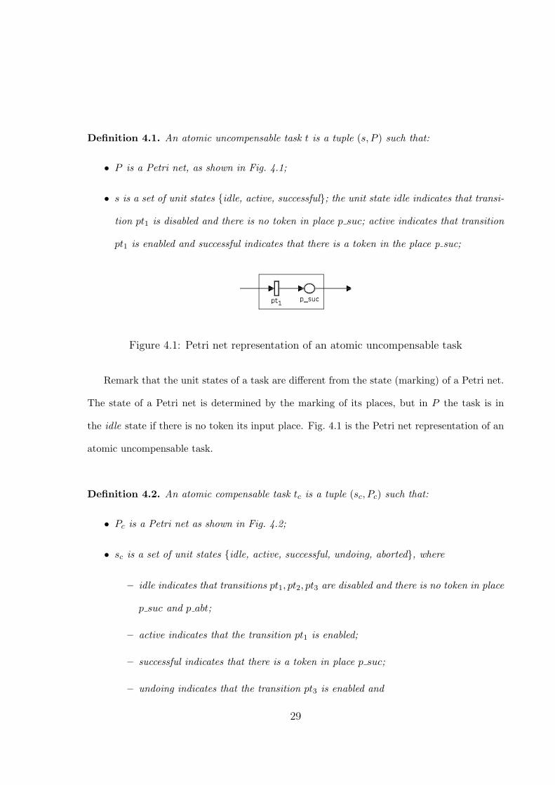
Definition 4.1. An atomic uncompensable task t is a tuple (s, P ) such that:
• P is a Petri net, as shown in Fig. 4.1;
• s is a set of unit states {idle, active, successful}; the unit state idle indicates that transi-
tion pt1 is disabled and there is no token in place p suc; active indicates that transition
pt1 is enabled and successful indicates that there is a token in the place p suc;
Figure 4.1: Petri net representation of an atomic uncompensable task
Remark that the unit states of a task are different from the state (marking) of a Petri net.
The state of a Petri net is determined by the marking of its places, but in P the task is in
the idle state if there is no token its input place. Fig. 4.1 is the Petri net representation of an
atomic uncompensable task.
Definition 4.2. An atomic compensable task tc is a tuple (sc, Pc) such that:
• Pc is a Petri net as shown in Fig. 4.2;
• sc is a set of unit states {idle, active, successful, undoing, aborted}, where
– idle indicates that transitions pt1, pt2, pt3 are disabled and there is no token in place
p suc and p abt;
– active indicates that the transition pt1 is enabled;
– successful indicates that there is a token in place p suc;
– undoing indicates that the transition pt3 is enabled and
29

– aborted indicates that there is a token in place p abt.
Figure 4.2: Petri net representation of an atomic compensable task
Fig. 4.2 gives the Petri net representation of an atomic compensable task. Solid lines
represent the forward flow and broken lines represent the compensation flow. The task tc
transits to the unit state active after getting a token in the input place of transition pt1.
The token can move to either p suc or p abt representing unit states successful or aborted,
respectively. The unit state aborted indicates an error occurred performing the task and
the effects was successfully removed. The backward (compensation) flow is started from this
point. Note that tc can transit to the unit state aborted either before or after the unit state
successful. We made a simplification for compensable tasks by excluding fail (failed), hap
(half-compensated) and cmp (compensated) states. In order to design a structurally sound
workflow (discussed in section 4.3 ) without explicit error handlers we have removed failed
and hap states from tc. On the other hand the state cmp overlapped with abort in tc.
A compensable task can be composed with other compensable tasks using the t-Calculus
operators. When a task executes, it performs some actions, and the execution of a task may
depend on some conditions. The formal definition of pre-condition and action are given below:
Definition 4.3. A term, σ, is defined using BNF as follows:
σ ::= c | χ | σ ⊕ σ, where ⊕ ∈ {+,−,×,÷},
30

c is a real number and χ is a real variable.
A pre-condition is a formula, ψpre, is defined as ψpre ::= σ ⋄ σ | (ψpre ⊎ ψpre), where
⋄ ∈ {<,≤, >,≥,==}, ⊎ ∈ {&&, ||} and σ is a term.
An action, ψact, of a task is an assignment defined as ψact ::= v = σ; v is called a mapsTo
variable and σ is a term
Definition 4.4. A compensable task, Tc, is recursively defined by the following well formed
formula:
Tc = tc({ψact}, {ψ′act}) | ({ψpre}Tc ⊙ {ψpre}Tc)
where tc is an atomic compensable task, {ψact} and {ψ′act} are the set of actions (forward and
compensation, respectively) of tc, {ψpre} is a set of pre-conditions of Tc and ⊙ ∈ {;, ||, ⊓, ⊗,
} is a t-Calculus operator defined for tasks in a manner identical to that for compensable
transactions in section 3.2.1 - 3.2.5.
Note that in our definition of atomic compensable task tc, we assume if activated, tc is either
completes successfully or fully compensate and as a result the backward handling operator (D),
forward handling operator (⊲) and programmable compensation operator (>) are not needed
here.
Any task can be composed with uncompensable and/or compensable tasks to create a new
task. As above, a task may be considered as a formula and we use BNF to represent the set
of “well formed” tasks or formulas.
Definition 4.5. A task, T, is recursively defined by the following BNF formula:
T ::= t{ψact} | Tc | ({ψpre}T ⊖ {ψpre}T )
where t is an uncompensable atomic task, {ψact} is the set of actions of t, {ψpre} is the set of
31

pre-conditions of T, Tc is a compensable task and ⊖ ∈ {∧,∨,×, •} is a control flow operator
defined as follows:
• T1 ∧ T2: T1 and T2 will be executed in parallel,
• T1 ∨ T2: T1 or T2 or both will be executed in parallel,
• T1 × T2: exclusively one of the task (either T1 or T2) will be executed,
• T1 • T2: T1 will be executed first then T2 will be executed.
A subformula of a well-formed formulae is also called a subtask. Any task which is built up
from the operators {∧,∨,×, •} is deemed as uncompensable. Thus if T1 and T2 are compensable
tasks, then T1;T2 denotes another compensable task while T1 • T2 denotes a task consisting of
two distinct compensable subtasks. We remark that the operators ∧,∨,× and • as well as the
t-Calculus operators ||,⊓, and ⊗ are all associative.
In order for the underlying Petri net construction to be complete, we add a pair of split
and join routing tasks for operators ∧, ∨, ×, ||, ⊓, ⊗, and and we give their graphical rep-
resentation in the following section (Fig. 4.3). Each of these routing tasks has a corresponding
Petri net representation, e.g., for the speculative choice operator Tc1 ⊗ Tc2 , the split routing
task will direct the forward flow to Tc1 and Tc2 ; the task that performs its operation first will
be accepted and the other one will be aborted.
We are now ready to make the formal definition of Compensable WorkFlow nets.
Definition 4.6. A Compensable Workflow net (CWF-net) CN is a tuple (i, o, T, Tc, F) such
that:
• i is the input condition,
• o is the output condition,
32

• T is a set of atomic tasks, split and join tasks
• Tc ⊆ T is a set consists of the compensable tasks, and T\Tc is the set of uncompensable
tasks,
• F ⊆ ({i} × T ) ∪ (T × T) ∪ (T × {o}) is the flow relation (for the net),
• The first compensable subtask of a compensable task is called the initial subtask; the
backward flow from the initial subtask is directed to the uncompensable task or the output
condition followed by the compensable task, and every task in a workflow is on a directed
path from i to o.
The elements of a workflow (i.e., tasks, input condition, output condition and flow rela-
tions) are called workflow components.
If a compensable task Tc in a CWF-net aborts, the system starts to compensate. After the
full compensation, the backward flow reaches the initial subtask of Tc and the flow terminates,
as the backward flow of an initial task of Tc is connected with an uncompensable task or the
output condition followed by Tc. The reader must distinguish between the flow relation (F ) of
the net, as above and the internal flows of the atomic (uncompensable and compensable) tasks.
A CWF-net such that Tc = T is called a fully Compensable workflow net (CWFf -net). To
organize a large CWF-net, it is convenient to divide a large CWF-net into small CWF-net’s.
Each small CWF-net representing a subformula is known as a subnet. A placeholder for the
subnet is used in the large CWF-net instead of a subformula. The placeholder is known as a
composite task. Example of a subnet may be found in chapter 8.
33

4.2 The compensable workflow modeling language
and its Petri net representation
We first present a graphical representation of tasks, then present the contruction principles for
modeling a compensable workflow. Our notation is inspired by YAWL [40], ADEPT2 [37] and
t-Calculus operators [29]. Fig. 4.3 gives a graphical representation of tasks, where t stands for
an uncompensable task and tc stands for a compensable task.
Figure 4.3: Graphical representation of CWML
34

Construction Principle: Construction principles for the graphical representation of tasks
are as follows:
• The operators [•, ; ] are used to compose the operand tasks sequentially. Atomic un-
compensable tasks and atomic compensable tasks are connected by a single forward flow.
Atomic compensable tasks are connected by a forward flow if they are composed using (•)
and by both a forward flow and a backward flow if they are composed using the sequential
operator (; );
• (The convention of ADEPT2 [37]) A pair of split and join routing tasks are used for tasks
composed by {∧, ∨, ×, ||, ⊓, ⊗, }. Atomic uncompensable tasks are connected with
split and join tasks by a single forward flow. Atomic compensable tasks are connected
with split and join tasks by two flows (forward and backward). The operators and their
corresponding split and join tasks are shown in Table 4.1;
• For those operators that are associative, an n-fold composition is represented using the
appropriate n-fold split and join. For example (t1∧t2)∧t3 which is the same as t1∧(t2∧t3)
is represented by t1 ∧ t2 ∧ t3, see Fig. 4.4.
If these principles are followed, the resulting graph is said to be “correct by construction”
(Terminologies borrowed from [37]).
Tasks composed with and composition are executed in parallel. In Fig. 4.3, we can see
the tasks ti and tn are composed with an “and” (∧) operator. It represents the formula
ti ∧ tn. Fig. 4.5 shows the Petri net representation of ti ∧ tn. In this figure ts (“and”
split) and tj (“and” join) are two routing tasks. During the execution, both tasks ti and
tn run in parallel.
Tasks composed with xor composition will be selected and activated depending on some
internal decisions. During execution, only one branch will be activated. In Fig. 4.3, we
35

Figure 4.4: n-fold split and join tasks
Figure 4.5: Petri net representation of and composition
36

can see tasks ti and in composed with an xor (×) operator, representing the formula ti
× tn. Fig. 4.6 shows the Petri net representation of ti × tn.
Figure 4.6: Petri net representation of xor composition
The or composition is used to decide between two or more tasks. Two tasks ti and tn
composed with an or choice (∨) are shown in Fig. 4.3. Fig. 4.7 shows the Petri net
representation of the ts (or split) and tj (or join) tasks. During execution, either ti and
tn both, or only ti will execute.
Figure 4.7: Petri net representation of or composition
Now we give the Petri net representation of compensable tasks and their composi-
tions. The behavioral dependencies described in chapter 3 for t-Calculus operators also
37

hold for the compensable task compositions.
Two compensable tasks tci and tcn can be composed with sequential composition as
shown in Fig. 4.3, which represents the formula tci ; tcn . Task tcn will be activated only
when task tci finishes its operations successfully. For the compensation flow, when tcn is
aborted, tci will be activated for compensation, i.e., to remove its partial effects. One of
the behavioral dependency for the composition tci ; tcn is (tci , suc) < (tcn , act), meaning
tcn will be activated iff tci was successful. It is obvious by inspection from the Petri
net representation of tci ; tcn from Fig. 4.8. The transition pt4 of tcn is connected with
the place p suc of tci by an incoming arc. In order to activate the transition pt4, there
has to be a token in place p suc of tci . Other behavioral dependencies for the sequential
composition can be found from the Petri net representation. Note that dependencies
which include state fal, hap, cmp does not hold here as we simplified the representation
of atomic task by removing those states.
Figure 4.8: Petri net representation of sequential composition
Tasks composed using internal choice will be selected and activated depending on some
internal decisions. During execution, only one branch will be activated and upon abort
the compensable flow will be executed. In Fig. 4.3, we can see tasks tci and tcn composed
with the internal choice composition, representing the formula tci ⊓ tcn . The basic
38
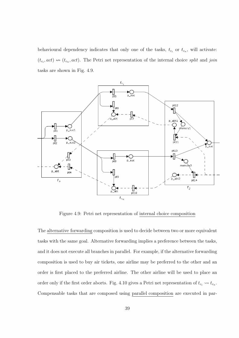
behavioural dependency indicates that only one of the tasks, tci or tcn , will activate:
(tci , act) = (tcn , act). The Petri net representation of the internal choice split and join
tasks are shown in Fig. 4.9.
Figure 4.9: Petri net representation of internal choice composition
The alternative forwarding composition is used to decide between two or more equivalent
tasks with the same goal. Alternative forwarding implies a preference between the tasks,
and it does not execute all branches in parallel. For example, if the alternative forwarding
composition is used to buy air tickets, one airline may be preferred to the other and an
order is first placed to the preferred airline. The other airline will be used to place an
order only if the first order aborts. Fig. 4.10 gives a Petri net representation of tci tcn .
Compensable tasks that are composed using parallel composition are executed in par-
39

Figure 4.10: Petri net representation of alternative forward composition
40

Figure 4.11: Petri net representation of parallel composition
41

allel. In Fig. 4.3, we can see the tasks tci and tcn which are composed in parallel. It
represents the formula tci || tcn . Compensable tasks tci and tcn will run in parallel but if
either of the tasks aborts, the other task will be aborted forcefully. The Petri net repre-
sentation of the parallel composition is shown in Fig. 4.11. Here we see two new places
PAR OK and FORCE ABORT , and two extra transition in each of tci and tcn . In the
Petri net representation, the split task ts activates both tci and tcn and produces a token
in place PAR OK. Note that parallel composition requires that if one branch aborts
then the other branch should be stopped to save time and resources. This is achieved
by these two extra places PAR OK and FORCE ABORT . In order to transit to the
successful state tci and tcn requires a token in place PAR OK. If any of the task from
tci or tcn is aborted, it consumes the token from the place PAR OK, and produces
a token in place FORCE ABORT . A token in place FORCE ABORT ensures that
other tasks (if activated) transit to the abort state.
The speculative choice composition is used to decide between two or more equivalent
tasks which have the same or similar goals. Speculative choice will execute two inde-
pendent tasks in parallel and will select the task which completes first. It is designed
to reduce the time complexity of a system by executing two tasks simultaneously which
could satisfy a requirement, but there is no preference between either tasks. The process
of buying air tickets can be modeled with speculative choice tasks. For example a system
orders tickets from two different airlines in parallel, then takes the one that is confirmed
first and cancels the other booking. In Fig. 4.3, we can see the tasks tci and tcn which
are composed by speculative Choice. It represents the formula tci ⊗ tcn . Fig. 4.12 shows
the Petri net representation of the speculative choice composition. Here we see two new
places SPEC OK and SPEC ABORT , and one extra transition in each of tci and tcn .
42

Figure 4.12: Petri net representation of speculative choice composition
43

Note that, if one task entered the aborted state before either task has completed then
the other task will continue to operate.
It is important to note that the speculative choice is a unique operator with respect to
the structural soundness of the whole Petri net. Let Tc = tc1⊗tc2 ...⊗tcn (n ≥ 2 is a finite
integer); Tc can be deemed as successful if tci (1 ≤ i ≤ n) succeeds and all other tasks
are compensated. However, only when Tc is aborted can the compensation flow proceed
to the task immediate preceding Tc. Therefore, the tokens in all of the compensated
subtasks will remain in their p abt places. As this situation will not affect the success
of the overall workflow, we consider these tokens as invisible and will ignore them in the
discussion of structural soundness (see the next section).
4.3 Analysis
The definition of soundness for CWF-nets is adapted from [43]. Informally, the sound-
ness of a CWF-net requires that for any case, the underlying Petri net will terminate
eventually, and at the moment it terminates, there is a token in the output condition and
all other places are empty. Formally, the soundness of CWF-nets is defined as follows:
Definition 4.7. A CWF-net CN = (i, o,T,Tc, F ) is sound (or structurally sound) iff,
considering the underlying Petri net:
1. For every state (marking) M reachable from the initial state Mi, there exists a
firing sequence leading from M to the final state Mf , where Mi indicates that there
is a token in the input condition and all other places are empty and Mf indicates
44

that there is a token in the output condition and all other places are empty;
2. Mf is the only state reachable from Mi with at least one token in the output con-
dition;
3. There are no dead transitions in CN . Formally: ∀t∈T , ∃M,M ′Mi →∗ M →t M ′
(where →∗ denotes 0 or more transitions).
Theorem 4.1. A CWF-net is sound.
Proof: Let CN be a CWF-net which consists of some uncompensable and compensable
tasks.
• Case 1, CN consists of only one uncompensable atomic task (t): as t is connected
to the input condition and the output condition, t will be activated by the input
condition and will continue the forward flow to the output condition. Hence the
flow terminates. This is obvious by inspection from Fig. 4.13, which shows the
Petri net representation of a CWF-net with an atomic task. This satisfies the
three conditions of soundness.
Figure 4.13: CWF-net with one atomic task
• Case 2, CN consists of only atomic uncompensable tasks composed by operators
{∧,∨,×, •}: according to the construction principle, every type of split task must
have the corresponding type of join task. This pair of split and join tasks provides
45

a safe routing for the forward flow; all the tasks of the workflow are on a path from
the input condition to the output condition, which ensures that there is no dead
transition in the workflow and the flow always terminates. This satisfies the three
condition of soundness. Therefore CN is sound.
• Case 3, CN includes some atomic uncompensable tasks and atomic compensable
tasks. First let us consider that CN has one atomic compensable task (tc). tc is
activated by some uncompensable atomic task or the input condition. If tc is suc-
cessful during the execution, it will activate the next task (or the output condition)
by continuing the forward flow. If tc is aborted, it will start the compensation flow.
As this is the only compensable task (by definition it is the initial task, see Def-
inition 4.7), the compensation flow is connected to the next uncompensable task
or to the output condition. It is easy to see from Fig. 4.14 that if tc is aborted,
the flow also terminates. An analogous argument holds if CN has one (nonatomic)
compensable task.
Figure 4.14: CWF-net with one compensable task
Now let us consider there is more than one compensable task in CN . For every
compensable task there is an initial subtask and the compensation flow of the
initial subtask is connected to the next uncompensable task or the output condition
46

(Fig. 4.15). If the compensable tasks do not abort, they will continue the forward
flow until the output condition is reached. If the composition of compensable tasks
is aborted, the compensation flow will reach the initial subtask, which will direct
the compensation flow to the next uncompensable task or the output condition.
Therefore it satisfies the conditions of the soundness. Thus CN is sound.
Figure 4.15: CWF-net with more compensable tasks
47

Chapter 5
Model checking and automated
translation
5.1 Model checking
Model checking is an automatic technique for verifying finite-state reactive systems.
The overall behaviour of a reactive system is modeled as a transition system. It can be
checked whether such a transition system is a model of a temporal logic formula, by a
technique originally developed by Clarke and Allen Emerson [14, 15]. Quielle and Sifakis
[35] independenty and shortly thereafter discovered a similar verification technique. This
technique, known as ‘model checking’, has several important advantages over mechanical
theorem provers or proof checkers for verification of circuits and protocols [13]. The
most important is that the procedure is highly automatic. Typically, the user provides
a high level representation of the model and the specification to be checked, written in a
suitable temporal logic. The model checker will either terminate with the answer true,
indicating that the model satisfies the specification, or give a counterexample execution
48
that shows one execution in which the formula is not satisfied. Such counterexamples
are particularly important in finding subtle errors in complex reactive systems.
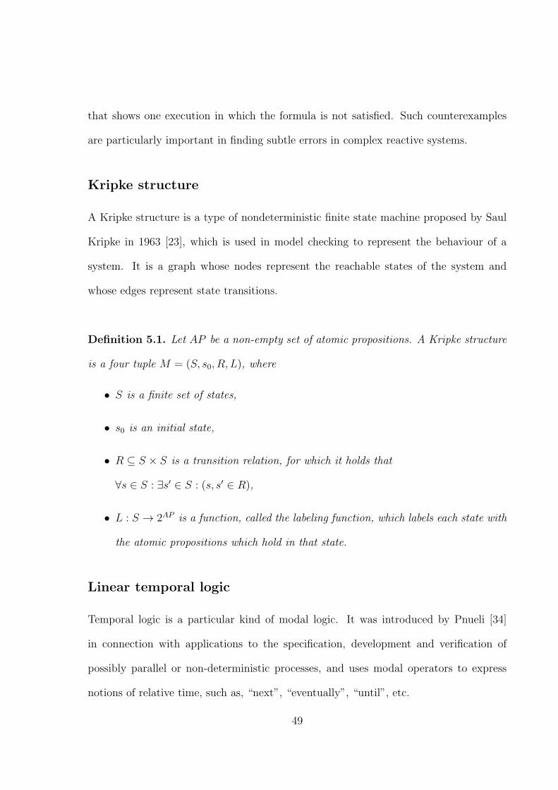
Kripke structure
A Kripke structure is a type of nondeterministic finite state machine proposed by Saul
Kripke in 1963 [23], which is used in model checking to represent the behaviour of a
system. It is a graph whose nodes represent the reachable states of the system and
whose edges represent state transitions.
Definition 5.1. Let AP be a non-empty set of atomic propositions. A Kripke structure
is a four tuple M = (S, s0, R, L), where
• S is a finite set of states,
• s0 is an initial state,
• R ⊆ S × S is a transition relation, for which it holds that
∀s ∈ S : ∃s′ ∈ S : (s, s′ ∈ R),
• L : S → 2AP is a function, called the labeling function, which labels each state with
the atomic propositions which hold in that state.
Linear temporal logic
Temporal logic is a particular kind of modal logic. It was introduced by Pnueli [34]
in connection with applications to the specification, development and verification of
possibly parallel or non-deterministic processes, and uses modal operators to express
notions of relative time, such as, “next”, “eventually”, “until”, etc.
49

LTL is a type of temporal logic which, in addition to classical logical operators, uses
the temporal operators such as: always (G), eventually (F ), until (U), and next time
(X) [22]. A well formed LTL formula, φ, is recursively defined by the BNF formula:
φ ::= p | ¬φ | φ → φ | φ ∧ φ | φ ∨ φ | X φ | F φ | G φ | φ U φ
where p is a propositional variable. The subset of LTL formula not containing the X
operator is denoted as LTL X . The semantics of LTL are defined with respect to a
Kripke model. Let M be a Kripke model, let π = s0, s1, .. be a path in the model M ,
let φ1 and φ2 be LTL formulas, and let p be a propositional variable. The notation
M,π � φ1 will be used to mean that formula φ1 holds or is satisfied along the path π
in the model M . We say a model M satisfies the formula φ, denoted as M � φ, iff all
of its runs, emanating from the initial state s0, satisfy φ. The satisfaction relation, �, is
formally defined as follows, where πi denotes the suffix of the path π starting at si:
M,π � p ⇐⇒ p ∈ L(s0)
M,π � ¬φ ⇐⇒ M,π 2 φ
M, π � φ1 ∨ φ2 ⇐⇒ M,π � φ1 or M,π � φ2
M,π � Xφ ⇐⇒ M,π1 � φ
M, π � Gφ ⇐⇒ ∀i ≥ 0 M,πi � φ
M, π � Fφ ⇐⇒ ∃i ≥ 0 M,πi � φ
M, π � φ1Uφ2 ⇐⇒ ∃k ≥ 0 M,πk � φ2 and ∀j, 0 ≤ j < k, M,πj � φ1
5.1.1 The DiVinE model checker and its modeling language
DiVinE is a parallel, distributed-memory explicit-state model checking tool for ver-
ification of concurrent systems. The tool employs the aggregate power of network-
interconnected clusters to verify systems whose verification is beyond the capability of
50

sequential tools [1]. The property to be specified is described by an LTL formula. Both
the system model and the LTL formula are represented by automata. Then the model
checking problem is reduced to detecting in the combined automaton graph whether
there is an accepting cycle, i.e., a cycle in which one of the vertices is marked ‘accepting’
with distributed algorithms assigning different portions of the state space to be explored
by different machines. DiVinE can (1) verify much larger system models; (2) finish
the verification in significantly less time for larger models (both in comparison with the
well-known explicit state LTL model checker SPIN [11]).
DVE is the modeling language of DiVinE. DVE is rich enough to describe systems
made of synchronous and asynchronous processes communicating via shared memory.
As with Promela (the modeling language of SPIN) a model described in DVE consists of
processes, message channels and variables. Each process, identified by a unique name,
consists of a list of local variable declarations, process state declarations, an initial state
declaration and a list of transitions, each of which starts using the keyword trans. Vari-
ables can be global (declared at the beginning of the DVE source code) or local (declared
at the beginning of a process), they can be of byte or int type. A transition transfers the
process from one state to another. The transition may contain a guard (which decides
whether the transition can be executed), a synchronization (which communicates data
with another process) and effects (which assign new values to local or global variables).
A guard contains the keyword guard followed by a Boolean expression and an effect
contains the keyword effect followed by a list of assignments.
51

5.2 Workflow translation to a model checker
Once a workflow is designed with compensable tasks, its properties can be verified by
model checkers such as SPIN, SMV or DiVinE. Modeling a workflow with the input
language of a model checker is tedious and error-prone. Leyla et al. [25] translated a
number of established workflow patterns into DVE for verifying properties of workflow
models. The translation process shown in [25] was a manual translation. Rabbi et
al. proposed an automatic translator in [36] which translates a graphical workflow
model constructed using the YAWL editor to DVE. Here we give the translation from
compensable workflow nets modeled in CWML to DVE. It was shown in chapter 4 that
each workflow task of CWML has a Petri net structure. If each workflow component of
a workflow model is represented by a Petri net model, the whole workflow is represented
by a Petri net model.
The NOVA Translator automatically translates a workflow from CWML to DVE,
the input language of the DiVinE model checker. In order to show that the translation
is correct, it is sufficient to show that a Petri net model (i.e., a compensable workflow
net modeled as a Petri net) can be correctly translated to a DiVinE model. Let us go
through some basic definitions first.
Definition 5.2. Let N be a Petri net structure. For each t ∈ T :
1. •t ={p | p F t } is called the preset of t,
2. t• ={p | t F p } is called the postset of t
Rule 1. The firing rules of a Petri net are as follows:
52

1. A transition t is said to be ready if each input place p of t is marked with at least
w(p,t) tokens, where w(p,t) is the weight of the arc from p to t,
t is ready iff, ∀p∈•t M(p) ≥ w(p, t) .
2. A ready transition may or may not fire (depending on whether or not the event
actually takes place).
3. A firing of a ready transition t removes w(p,t) tokens from each input place p of
t, and adds w(t,p) tokens to each output place p of t, where w(t,p) is the weight of
the arc from t to p.
The set of all ready transitions for a marking M is denoted by Tready(M). If a
transition t is ready with marking M , ready(t,M) is true, otherwise it is false.
Definition 5.3. Let N be a Petri net structure, and M a marking of N. The marking
M′ to N, obtained from M by firing transaction t, where t ∈ Tready(M), written M [〉t M′,
is defined as:
∀p∈PNM ′(p) =
M(p) + w(t, p) if p ∈ t•
M(p)− w(p, t) if p ∈ •t
M(p) otherwise
The pre-condition (ψpre) of a task T is the condition for its execution. The pre-
condition ψpre is encoded into the Petri net model as w(p, t). On the other hand, the
action ψact is encoded into the Petri net as w(t, p). let π = M0[〉tjM′1[〉tk .... be a path
in a Petri net model PM = (N,M0), let φ1 and φ2 be LTL formulas, and let p be a
propositional variable. The notation PM, π � φ1 will be used to mean that formula φ1
53

holds or is satisfied along the path π in the model PM . We say a model PM satisfies
the formula φ, denoted as PM � φ, iff all of its runs, emanating from the initial marking
M0, satisfy φ. The satisfaction relation, � for Petri net, is defined in a manner similar
to that for the satisfaction relation of a Kripke model in section 5.1. PM, π � p iff
PM,M0 � p which means that there is a token in place p. Now we define the DiVinE
model and provide the translation principle:
Definition 5.4. A DVE Petri net model is an 8-tuple, DM = (V, Proc, T,G,E, F,W, S0)
where:
• V = {var1, var2, ..} is a finite set of variables,
• Proc = {Proc1, P roc2, ...} is a finite set of processes,
• T = {t1, t2, ...} is a finite set of transitions,
• G ⊆ (V × T ) is a set of guards,
• E ⊆ (T × V ) is a set of effects,
• F = (G ∪ E) is a set of flow relations,
• W : F → {1, 2, 3...} is a weight function,
• S0 : V → {1, 2, 3, ...} is the initial marking.
A 7-tuple D = (V, Proc, T,G,E, F,W ) is called a DVE Petri net structure (no specific
initial marking).
54

Remark: Generally a DVE model can have other features (i.e., channels, arrays, etc.)
[1] but we do not require these features here.
Definition 5.5. The state Si of a DVE Petri net model is determined by:
Si = {(varp0, Si(varp0)), (varp1, Si(varp1)), . . (varpn, Si(varpn))}, where varpv is
a DVE variable, and Si(varpv) is the value of the variable varpv .
5.2.1 Petri net to DVE translation
Translation Principle 1. A Petri net model PM (N,M0) is translated to a DVE Petri
net model DM (D,S0) by the following rules:
• for each place pi ∈ PN , there corresponds a variable vari in DM ; the initial value
of the variables are set with the initial marking M0 of the Petri net,
S0(vari) =M0(pi).
• for each transition ti ∈ TN , there corresponds a process Proci in DM ; Proci has
a transition t′i; the guard and effect of t′i are determined by the weight function of
ti;
• a transition t′ in a DVE Petri net model is ready if it satisfies the following guard
condition:
∀v∈•t′S(varv) ≥ w(v, t′), where •t′ = {v | v G t′} and w(v, t′) = w(p, t);
if t′ is ready at state S, ready(t′, S) is true, otherwise it is false;
55

• the firing of a ready transition t′ changes the state of a DVE Petri net model. The
new state S ′ is obtained from S by the firing of t′; the path S [〉t′ S′ is defined
formally as:
∀v∈V S′(v) =
S(v) + w(t′, v) if v ∈ t′•
S(v)− w(v, t′) if p ∈ •t′
S(v) otherwise
Note that the translated weight function preserves the source Petri net’s weight
information; hence ∀p∈PNw(p, t) = w(varp, t
′) and ∀p∈PNw(t, p) = w(t′, varp);
Note that the satisfaction relation, � for a DVE model DM = (D,S0) is identical to the
satisfaction relation of a Petri net model. Algorithm 1 is the algorithm to translate a
Petri net model to DVE.
We will describe the translation using a simple example. Fig. 5.1 shows a Petri net
with four places P1, P2, P3, P4, two transitions t1, t2, six arcs (p1, t1), (p2, t1), (p2,
t2), (t1, p3), (t1, p4), (t2, p4). Initially p1 and p2 have 4 and 3 tokens respectively.
Each arc has a weight that is specified above the arc.
Figure 5.1: A Petri net
The translated DVE model will have four variables (i.e., var p1, var p2, var p3,
var p4 ). var p1 and var p2 will be assigned with 4 and 3 as initial values. The tran-
56
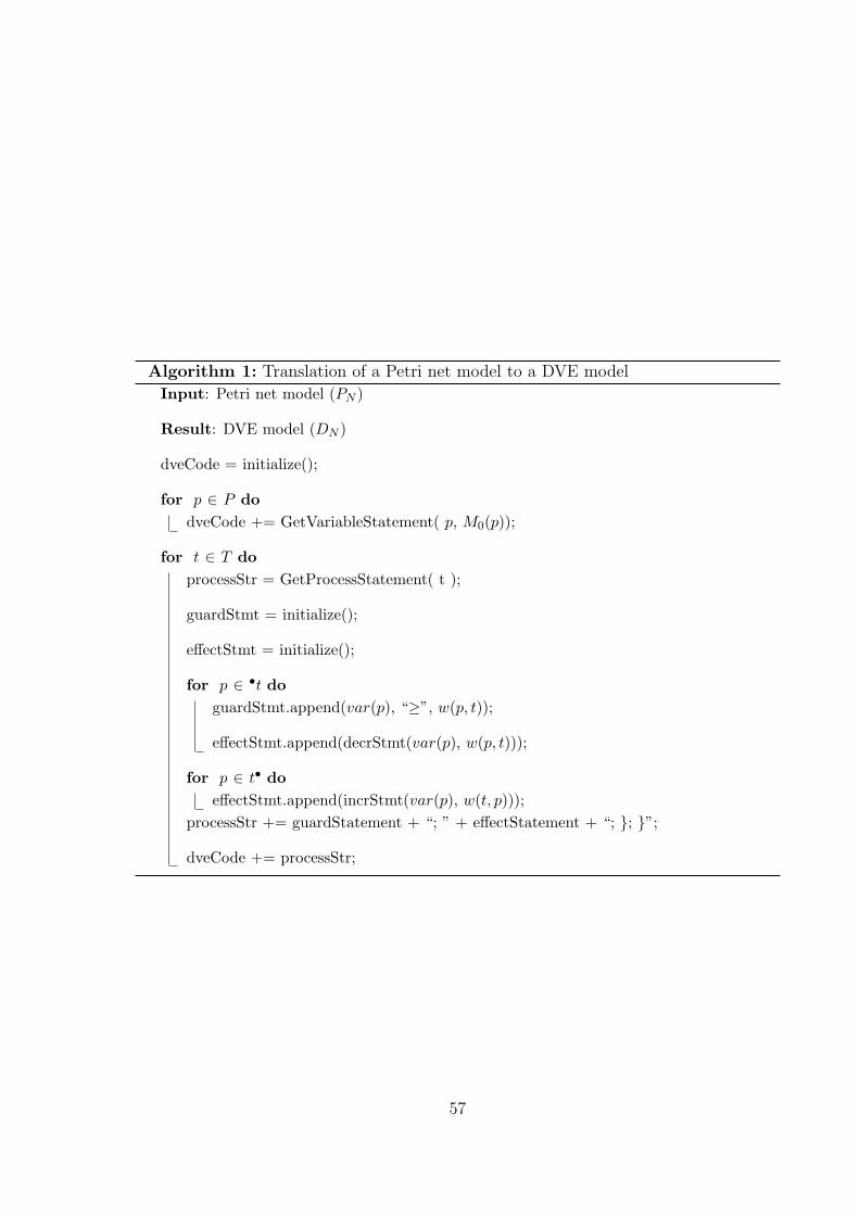
Algorithm 1: Translation of a Petri net model to a DVE model
Input: Petri net model (PN )
Result: DVE model (DN )
dveCode = initialize();
for p ∈ P do
dveCode += GetVariableStatement( p, M0(p));
for t ∈ T do
processStr = GetProcessStatement( t );
guardStmt = initialize();
effectStmt = initialize();
for p ∈ •t do
guardStmt.append(var(p), “≥”, w(p, t));
effectStmt.append(decrStmt(var(p), w(p, t)));
for p ∈ t• do
effectStmt.append(incrStmt(var(p), w(t, p)));
processStr += guardStatement + “; ” + effectStatement + “; }; }”;
dveCode += processStr;
57

sitions t1 and t2 will be translated as processes Proc t1 and Proc t2, respectively. For
our example in Fig. 5.1, the guard condition of process Proc t1 will be (var p1 ≥ 2 and
var p2 ≥ 1 ), as transition t1 has two incoming arcs connected with p1 and p2 where
w(p1, t1) = 2 and w(p2, t1) = 1 (see Fig. 5.1). On the other hand, Proc t1 will increase
the value of var p3 and var p4 by 2 and 1 respectively as w(t1, p3) = 2 and w(t1, p4)
= 1. The DVE code for the DVE Petri net model shown in Fig. 5.1 is provided here:
int var_p1 = 4;
int var_p2 = 3;
int var_p3 = 0;
int var_p4 = 0;
process Proc_t1{
state tr;
init tr;
trans
tr -> tr{ guard var_p1 >= 2 & var_p2 >= 1 ;
effect var_p1 = var_p1 - 2, var_p2 = var_p2 - 1,
var_p3 = var_p3 + 2, var_p4 = var_p4 + 1;
};
}
process Proc_t2{
state tr;
init tr;
trans
tr -> tr{ guard var_p2 >= 1 ;
58

effect var_p2 = var_p2 - 1,
var_p4 = var_p4 + 1;
};
}
system async;
5.2.2 Proof of correctness
Definition 5.6. Let PM (N,M0) be a Petri net model and DM (D,S0) be a DVE Petri
net model. A Petri net state Mi of PM, and a DVE state Si of DM are equivalent,
denoted Mi∼= Si iff:
∀p∈PNMi(p) = Si(varp), where varp is the variable corresponding to place p
Definition 5.7. A path π = M0[〉tjM1[〉tk ... in a Petri net model PM and path π′ =
S0[〉t′jS1[〉t′k... in a DVE Petri net model DM correspond written (π ∼= π′) iff ∀i ≥ 1
Mi∼= Si .
Remark: If two paths π and π′ correspond then for all i, πi and π′i correspond.
Definition 5.8. A Petri net model PM (N,M0) and a DVE Petri net model DM
(D,S0) are equivalent (PM ∼= DM) iff:
• M0∼= S0,
59

• for every path starting from M0 (π =M0[〉tiM1[〉tj ...) there is a corresponding path
starting from S0, (π′ = S0[〉t′iS1[〉t′j ...) and for every path starting from S0 there is
a corresponding path starting from M0.
Theorem 5.1. If DM is the DVE translation of a Petri net PM , then PM ∼= DM .
Proof: Let PM = (N,M0) be a Petri net model and DM = (D,S0) be the DVE
model that we get after the translation of PM .
S0 = {(varp0 , a1), (varp1 , a2), ...(varpn , an)}, where
∀pi,0≤i≤nS0(varpi) =M0 (pi)
Let π be a path in PM , we will show by induction on the number of transitions in π
that π′, the translation of π, corresponds to π.
Base Case: Show: M0∼= S0.
The initial marking M0 of PM and S0 of DM are equivalent as:
∀p∈PNM0(p) = S0(varp)
hence M0∼= S0; this proves our base case.
Induction step: Show that if for all paths π of length k in PM there is a corresponding
path π′ of length k in DM , then for all path π of length k + 1 in PM , there is a
corresponding path π′ of length k + 1 in DM .
Let us assume that for any path π of length k, Mk∼= Sk (induction hypothesis). So we
have
∀t∈Tready(Mk)ready(Proct, Sk) = true.
60

If any of the transition t ∈ Tready(Mk) fires, we will get the following changes to the
marking:
∀p∈•tMk+1(p) =Mk(p)− w(p, t), and ∀p∈t•Mk+1(p) =Mk(p) + w(t, p).
Similarly the DVE process Proct for the transition t′ will change the values of the
variables as follows:
∀v∈•t′Sk+1(v) = Sk(v)− w(v, t′), and ∀v∈t′•Sk+1(v) = Sk(v) + w(t′, v).
Again, by Translation Principle 1 (see section 5.2.1), we may conclude:
∀p∈PNMk+1(p) = Sk+1(varp).
hence Mk+1∼= Sk+1; this proves our induction step. Therefore it is established that for
every path π ∈ PM starting from M0, there is a corresponding path π′ ∈ DM starting
from S0.
Similarly we can show that if DM is the translation of PM , where S0 corresponds to
M0, then for every path π′ in DM starting from S0, there is a corresponding path π in
PM starting from M0. Let π′ be a path in DM starting from S0; we will show that π′
corresponds to π by doing induction on the number of transitions in π′
Base Case: Show S0∼= M0.
By the Translation Principle 1, the initial state S0 of DM and the initial marking
M0 of PM are equivalent. Which proves our base case.
Assuming for all path π′ of length k in DM there is a corresponding path π of length k
in PM (induction hypothesis), we get Sk∼= Mk. For each ready transition t′ ∈ Tready(Sk)
there is a transition t in PM which is ready for marking Mk. If any transition t′ ∈
Tready(Sk) fires, it will make the following changes in DM :
∀v∈•t′Sk+1(v) = Sk(v)− w(v, t′) and ∀v∈t′•Sk+1(v) = Sk(v) + w(t′, v).
61

The firing of t′’s corresponding transition t in PM will make the following changes:
∀p∈•tMk+1(p) =Mk(p)− w(p, t) and ∀p∈t•Mk+1(p) =Mk(p) + w(t, p).
As ∀v∈V Sk+1(v) =Mk+1(pv), Sk+1∼= Mk+1, which proves our induction step.
Therefore we can conclude that for any path π′ = S0[〉t′iS1[〉t′j ... in DM starting from S0,
there is a corresponding path π = M0[〉tiM1[〉tj ... starting from M0 in PM . As both of
the models have the same state space, so PM ∼= DM .
Proposition 1. Let π be a path in PM corresponding to a path π′ in DM . Then for
any LTL formula φ, π � φ iff π′ � φ.
Proof: By structural induction on the formula φ.
The p be a propositional variable and let σ and τ be propositional formulas.
Let π =M0[〉tiM1[〉tjM2...
π � p iff M0 � p iff S0 � p (since M0∼= S0) iff π
′ � p
π |= ¬σ iff M0 � ¬σ iff M0 2 σ iff S0 2 σ (induction) iff S0 � ¬σ iff π′ � ¬σ
The case φ = σ ∨ τ is analogous to the above.
Now consider formulas with temporal operators:
π � Xσ iff π1 � σ iff π1′ � σ (since π corresponds to π′ so π1 corresponds to π1′ , by
the induction hypothesis) iff π′ � Xσ
π � σUτ iff ∃k such that ∀0≤i<kπi � σ and πk � τ . Since π corresponds to π′, πi
corresponds to πi′ and πk corresponds to πk′ . So by induction, ∀0≤i<kπi′ � σ and πk′ � τ .
Hence π′ � σUτ .
The cases π = F σ and π = G σ are established in a similar manner.
The case π′ � φ′ implies π � φ is established similarly.
62

Theorem 5.2. Let φ be an LTL formula, and let PM ∼= DM . Then PM � φ iff
DM � φ.
Proof: Suppose PM � φ for some LTL formula φ. Then for all paths π in PM starting
at M0, π � φ . We wish to show that for all paths π′ in DM starting at S0, π′ � φ .
Let π′ be a path in DM starting at S0. Since PM ∼= DM , there is a path π in
PM starting at M0 and corresponding to π′. By assumption, π � φ. The previous
proposition allows us to conclude that π′ � φ.
Analogously we may show that if DM � φ then PM � φ.
63

Chapter 6
Workflow model reduction
Model checking [22] or other such verification techniques are required to ensure that the
process model exhibits the desired behavior. While current model checkers are much
more powerful than their predecessors, they still suffer from the state explosion problem
[22]. This chapter describes a workflow reduction algorithm. The workflow reduction
is based on the dependency relation that exists among task variables and the order of
execution of the tasks. This reduction method specifies which tasks or variables should
be included in the reduced model and which should not. Work related to handling the
state explosion are presented in the following section.
6.1 Related work
6.1.1 Partial order reduction
The partial order [22] reduction reduces the size of the state space that needs to be
searched by model checking algorithms. It constructs a reduced state graph where the
behaviors (i.e., paths) of the reduced graph are a subset of the behaviors of the full state
64

graph. It ensures that if a behavior is not present in the reduced state graph, then a
behavior equivalent with respect to a property being verified is included. This reduction
technique is best suited for asynchronous systems. We will discuss this method in detail
as it served as inspiration for our results.
A common observation about concurrent asynchronous systems is that the inter-
leaving model imposes an arbitrary ordering between concurrent events. To avoid dis-
criminating against any particular ordering, the events are interleaved in all possible
ways. The ordering between independent transitions is often largely meaningless. How-
ever, common specification languages, including many temporal logics, can distinguish
between behaviors that only differs in this manner. Partial order reduction aims to
take advantage of the cases where the specifications do not distinguish between such
behaviors. In these cases, the partial order reduction only checks a subset of the be-
haviors. However, it checks sufficiently many of them to guarantee the soundness of the
verification [22].
Definition 6.1. A state transition system is a quadruple (S,T,S0,L) where
• S is the set of states,
• S0 is the set of initial states,
• L : S → 2AP is the labeling function that labels each state with a set of atomic
propositions,
• T is a set of transitions such that for each α ∈ T, α ⊆ S × S.
A Kripke structure M = (S,R, S0, L) may be obtained by defining R so that R(s, s′)
holds when there exists a transition α ∈ T such that α(s, s′). For a transition α ∈ T , we
65

say that α is enabled in a state s if there is a state s′ such that α(s, s′) holds. Otherwise
α is disabled in s. The set of transitions enabled in s is enabled(s).
Depth First Search (DFS) with partial order reduction
The reduction is performed by the DFS used to construct the state graph, as in Algorithm
2. The search starts with an initial state s0 and proceeds recursively. For each state s
it selects only a subset ample(s) of the enabled transitions enabled(s), rather than the
full set of enabled transitions, as in the full state space construction. The DFS explores
only successors generated by these transitions.
Algorithm 2: Depth-first search with partial order reduction [22]
hash(s0);
set on stack(s0);
expand state(s0);
procedure expand state(s)
work set(s) := ample(s);
while work set(s) is not empty do
let α ∈ work set(s);
work set(s) := work set(s) \ {α};
s′ := α(s);
if new(s′) then
hash(s′);
set on stack(s′);
expand state(s′);
create edge(s, α, s′);
set completed(s);
end procedure
66

Definition 6.2. An Independence relation I ⊆ T × T is a symmetric, antireflexive
relation, satisfying the following two conditions for each state s ∈ S and for each (α,β)∈
I:
• Enabledness: If α , β ∈ enabled(s) then α ∈ enabled(β(s)).
• Commutativity: α , β ∈ enabled(s) then α(β(s)) = β(α(s)).
Figure 6.1: Execution of independent transitions
The Dependency relation D is the complement of I, namely D = (T× T ) \ I.
A transition α ∈ T is invisible with respect to a set of propositions AP ′ ⊆ AP if for
each pair of states s, s′ ∈ S such that s′ = α(s), L(s) ∩ AP ′ = L(s′) ∩ AP ′. In other
words, a transition is invisible when its execution from any state does not change the
value of the propositional variable in AP ′. A transition is visible if it is not invisible.
Figure 6.2: If AP’ = {p} then α is invisible
67

Stuttering equivalent paths
Two infinite paths σ = s0α0→ s1
α1→ ... and ρ = r0β0→ r0
β0→ ... are stuttering equivalent (
σ ∼st ρ) if there are two infinite sequences of positive integers 0 = i0 < i1 < i2 < ... and
0 = j0 < j1 < j2 ... such that for every k ≥ 0,
L(sik) = L(sik+1) = ... = L(sik+1−1) = L(rjk) = L(rjk+1) = ... = L(rjk+1−1)
Figure 6.3: Two stuttering equivalent paths
In other words, the paths can be partitioned into infinitely many blocks, such that
the states in the kth block of one are labeled the same as the states in the kth block of
the other. The blocks can have different lengths. An LTL formula f is invariant under
stuttering if and only if for each pair of paths π and π′ such that π ∼st π′ ,
π| = f if and only if π′| = f
We denote the subset of the logic LTL without the next time operator by LTL−X .
Theorem 6.1. Any LTL−X property is invariant under stuttering.
The theorem is proved using a simple induction on the size of the LTL formula [22].
Partial order reduction for LTL−X
When the specification is invariant under stuttering (i.e., formula in LTL−X), partial
order reduction can use commutativity and invisibility which avoids generating some
68

states. In [13] author suggests a systematic way of selecting an ample set of transitions
for any given state. The ample sets will be used by the DFS algorithm in Algorithm
2 to construct a reduced state graph so that for every path not considered by the DFS
algorithm there is a stuttering equivalent path that is considered. This guarantees that
the reduced state graph is stuttering equivalent to the full state graph. There are four
conditions for selecting ample(s) ⊆ enabled(s) by which we can make sure that the
satisfaction of the LTL−X specification is preserved [22].
Condition C0: If a state has at least one successor, then the reduced state graph also
contains a successor for this state; i.e.:
C0 ample(s) = φ if and only if enabled(s) = φ
Condition C1: Along every path in the full state graph that starts at s, the following
condition holds:
a transition that is dependent on a transition in ample(s) cannot be executed without
a transition in ample(s) occurring first.
Note: C1 refers to paths in the full state graph
Condition C2 [Invisibility]: If s is not fully expanded, then every α ∈ ample(s) is
invisible.
Condition C3 [Cycle condition]: A cycle is not allowed if it contains a state in which
some transition α is enabled, but is never included in ample(s) for any state s on the
cycle.
The complexity of checking the conditions
Condition C0 for a particular state can be checked in constant time. Condition C2 is also
simple to check, by examining the transitions in the set. Condition C1 is a constraint
69

that is not immediately checkable by examining the current state of the search, in that
it refers to future states (some of which need not even be in the reduced state graph).
The next theorem shows that, in general, checking C1 is at least as hard as searching
the full state space.
Theorem 6.2. Checking Condition C1 for a state s and a set of transitions T ⊆
enabled(s) is at least as hard as checking Reachability for the full state space.
Proof: see [13].
6.1.2 Other work
In [38] [39] the authors provided reduction rules as a stand alone approach to reduce
the complexity of the process model. In [45] [31] the authors applied similar reduction
techniques as an engineering approach. A reduction procedure for BPMN graphs was
provided in [10] but the authors did not provide any reduction algorithm for workflows
with variables. In none of these approaches is there a proof of stuttering equivalence.
6.2 Workflow model reduction
In this section we will discuss a workflow reduction algorithm for the CWML. The reduc-
tion algorithm is based on the property subject to verification and the workflow model.
The workflow reduction method reads both the workflow file and the file containing an
LTL specification (called the LTL-property file) and based on the specification that we
want to verify, reduces the workflow. The reduced workflow is then translated into DVE,
the input language of DiVinE. The algorithm is provided in this section. In chapter 4
70
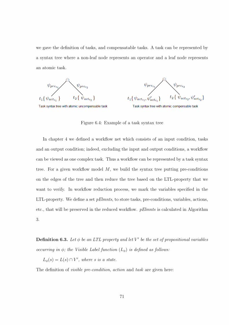
we gave the definition of tasks, and compensatable tasks. A task can be represented by
a syntax tree where a non-leaf node represents an operator and a leaf node represents
an atomic task.
Figure 6.4: Example of a task syntax tree
In chapter 4 we defined a workflow net which consists of an input condition, tasks
and an output condition; indeed, excluding the input and output conditions, a workflow
can be viewed as one complex task. Thus a workflow can be represented by a task syntax
tree. For a given workflow model M , we build the syntax tree putting pre-conditions
on the edges of the tree and then reduce the tree based on the LTL-property that we
want to verify. In workflow reduction process, we mark the variables specified in the
LTL-property. We define a set pElmnts, to store tasks, pre-conditions, variables, actions,
etc., that will be preserved in the reduced workflow. pElmnts is calculated in Algorithm
3.
Definition 6.3. Let φ be an LTL property and let V ′ be the set of propositional variables
occurring in φ; the Visible Label function (Lφ) is defined as follows:
Lφ(s) = L(s) ∩ V ′, where s is a state.
The definition of visible pre-condition, action and task are given here:
71

Definition 6.4. (visible pre-condition, action and task) (a) A pre-condition
(ψpre) is visible iff there exists a variable in ψpre which is in pElmnts. If a pre-condition
ψpre is visible, we say visible(ψpre) = true.
(b) An action (ψact) is visible iff the mapsTo variable of ψact is in pElmnts. If an action
ψact is visible, we say visible(ψact) = true.
(c) A task t is visible iff there exists an action of t, ψactt, such that visible(ψactt) = true.
If a task t is visible, we say visible(t) = true.
If a pre-condition, task or action is not visible, we say that it is invisible. The reduction
algorithm is provided in Algorithm 3. For a given workflow model M and LTL-property
φ, the algorithm constructs a syntax tree τ fromM . The set pElmnts is initialized with
the empty set and the variables occurring in the specification φ are inserted into it. Then
the algorithm recursively inserts those tasks, actions, and pre-conditions into pElmnts
which are visible in τ and continues until there are no visible elements left in τ to be
added. The algorithm constructs the reduced syntax tree τ ′ and the reduced model M ′
using the elements in pElmnts. The construction of M ′ from τ ′ is straightforward as a
task syntax tree represents formula and a workflow can be generated from the formula.
Example
Fig. 6.5 gives a workflow model Mex containing 11 atomic tasks. The property we want
to verify for this workflow is: G((v1 == 1) → F (v2 == 1)), meaning if v1 is set with
value ‘1’, v2 will eventually be set with value ‘2’. Task pre-conditions are shown above
the edges and task actions are shown below the tasks. We will reduce this workflow
according to the reduction algorithm.
The following formulas represent the workflow Mex.
72

Algorithm 3: Reduction AlgorithmInput: Workflow Model M, LTL specification φ
Result: Reduced Workflow Model M ′
construct syntax tree τ ; set pElmnts = empty;
for v ∈ φ do
pElmnts.add(v);
size = 0;
while size != pElmnts.size do
for ψpre ∈ τ do
if visible(ψpre) = true then
pElmnts.add(ψpre);
for task t ∈ τ do
if visible(ψactt) = true then
pElmnts.add(t); pElmnts.add(ψactt);
pElmnts.add(ψpret); visitingTask := t.parentNode;
while visitingTask != rootNode do
pElmnts.add(visitingTask); pElmnts.add(ψprevisitingTask);
if visitingTask is an XOR or OR task then
leftNode := visitingTask.leftChild;
rightNode := visitingTask.rightChild;
pElmnts.add(ψpreleftNode); pElmnts.add(ψprerightNode
);
visitingTask = visitingTask.parentNode;
if size = pElmnts.size then
set tree τ ′ := τ ;
for task t ∈ τ ′ do
if t /∈ pElmnts then
ψactt := NIL; t := NIL; // take out stuff marked as NIL
for ψpre ∈ τ ′ do
if ψpre /∈ pElmnts then
ψpre := NIL;
generate M ′ by visiting τ ′;
return;
size = pElmnts.size;
73

Figure 6.5: The workflow Mex
T4 = T5× T6
T8 = ((T11 • T12) ∨ T10) ∨ (T9 • T17)
T1 = (T2 • T8) ∧ (T3 • T4 • T16)
T = (T1 • T15)
Fig. 6.6 shows the task syntax tree for Mex. The pre-conditions of tasks T5 (v1! = 1)
and T6 (v1 == 1) are inserted into pElmnts as the variable v1 occurs in the given LTL
specification; this is indicated by thick lines in Fig. 6.6. Tasks T3, T6 and T9 are visible
as they have visible actions. Paths from T3, T6 and T9 to the root node become visible
and all the pre-conditions along the way become visible (represented by thick lines). As
v4 becomes a visible variable, the pre-conditions (v4 == 1), (v4 == 2), (v4! = 1) become
visible. Task T2 becomes a visible task as it has an action (v4 = {1, 2, 3}) which changes
the value of a visible variable. Nothing more is visible in the tree, hence we stop inserting
elements into pElmnts.
The reduced workflow M ′ex is shown in Fig. 6.7. M ′
ex has fewer concurrent tasks but
74

Figure 6.6: The task syntax tree for Mex
will provide the same verification result for the given LTL specification (see the proof
of stuttering equivalence in the following section). Experimental result shows that the
property does not hold and one of the counter examples is given below:
s0T1→ s1
T3→ s2
T2→ s3
T8→ s4
T9→ s5
T4→ s6
T7→ s7...
The counter example shows that the variable v1 is set with the value ‘1’ in task T3, and
it is reset with another value (i.e., v1 = 2) in task T9; for this execution the property
G((v1 == 1) → F (v2 == 1)) does not hold in M ′ex and hence not in Mex.
6.3 Proof of stuttering equivalence
If each workflow component of a workflow model is represented by a Petri net model,
the whole workflow is represented by a Petri net model. A CWFnet has one initial state,
which is the initial marking of the Petri net.
Definition 6.5. (adapted from [22]) Two infinite paths σ = s0α0→ s1
α1→ ... and
75

Figure 6.7: The reduced workflow M ′ex
ρ = r0β0→ r0
β0→ ... are stuttering equivalent ( σ ∼st ρ) with respect to the LTL-formula
φ if there are two infinite sequences of positive integers 0 = i0 < i1 < i2 < ... and 0 =
j0 < j1 < j2 ... such that for every k ≥ 0,
Lφ(sik) = Lφ(sik+1) = ... = Lφ(sik+1−1) = Lφ(rjk) = Lφ(rjk+1) = ... = Lφ(rjk+1−1)
(where Lφ is as defined in Definition 6.3).
Thus σ ∼st ρ w.r.t φ iff the paths can be partitioned into infinitely many blocks,
such that the states in the kth block of σ are lableled (w.r.t φ) the same as the states
in the kth block of ρ.
Definition 6.6. (adapted from [13]) Two workflow models M and M ′ are stuttering
equivalent (M ∼st M′) with respect to an LTL formula φ, iff:
• Lφ(s0) = Lφ(r0), where s0, r0 are the initial states of M and M ′ respectively, i.e.,
M and M ′ have the same set of inital states (one each);
• For each path π of M that starts from the initial state s0 of M there exists a path
76

σ of M ′ from the initial state r0 w.r.t φ such that π ∼st σ, and;
• for each path σ of M ′ that starts from the initial state r0 of M ′ there exists a path
π of M from the initial state s0 w.r.t φ such that σ ∼st π.
Thus, in order to show that the reduction algorithm is correct it is sufficient to show
that M and M ′ are stuttering equivalent. We begin with some Lemmas.
Lemma 1. Any task below an invisible pre-condition of a task syntax tree is invisible.
Proof: We will prove this by contradiction. Let tv be a visible task below an invis-
ible pre-condition ψprei . As tv is a visible task, then according to Algorithm 3, all
pre-conditions from tv to the root node are recursively added to pElmnts. From the
definition of visible pre-condition, we know that a pre-condition ψpre which is in pElmnts
is a visible pre-condition. Thus if ψprei belongs to the path from tv to the root node, it
cannot be invisible.
Lemma 2. An invisible task cannot change the flow of a visible task.
Proof: By definition, an invisible task contains only invisible actions. An invisible
action ψacti cannot change the value of a visible property. So an invisible action can
only change invisible pre-conditions. From Lemma 1 we know that an invisible pre-
condition can only change the flow of an invisible task. Thus an invisible action cannot
change the control flow of a visible task, which proves that an invisible task cannot
change the control flow to a visible task.
Theorem 6.3. A Workflow model M and its reduced modelM ′ are stuttering equivalent.
77

Proof: Let φ be an LTL specification and AP ′ be the set of propositional variables
in φ. The Workflow model M is reduced to M ′ according to the Workflow Reduction
Algorithm with respect to the specification φ. τ and τ ′ are two syntax trees representing
workflows M and M ′ respectively. We will prove this theorem by doing structural
induction on the number of atomic tasks of τ .
Base Case: Let M1 be a model such that the syntax tree τ1 has one atomic task
t1{ψactt1}. We have to show that M1 ∼st M
′1 There are two possibilities:
1. t1{ψactt1} is visible: Since τ1 has one vertex, and it is visible, there is no reduction.
Here, τ ′ and τ are same; thus M and M ′ are identical.
2. t1{ψactt1} is invisible: In this case τ ′1 is empty. The only possible path in M1 is
(π = s0t1→ s1) which is stuttering equivalent to the initial state r0 of M ′
1 as Lφ(s0) =
Lφ(s1) = Lφ(r0); thus M1 ∼st M′1.
In either situation, M1 ∼st M′1.
Induction: Assume that for all models Mk with k atomic tasks in τk, Mk ∼st M′k; we
have to show that, for all models Mk+1 with k+1 atomic tasks in τk+1, Mk+1 ∼st M′k+1.
To get a model with k+1 atomic tasks we can build one from a model with k atomic
tasks, by replacing an atomic task by a task in the form t1{ψactt1} ⊖ t2{ψactt2
} where ⊖
∈ {•, ∧, ×, ∨, ;, ||, ⊓, ⊗, }. Equivalently we can take a syntax tree with k leaf nodes
and replace a leaf t1 with the subtree with two leaf nodes t1 and t2. Let a leaf node
ti{ψactti}(1 ≤ i ≤ k) be replaced by a control flow operator (⊖n) in τk to get a tree τk+1
with k + 1 atomic tasks. Let tn{ψacttn} be a new task added to the right branch of ⊖n
while ti{ψactti} is added to the left branch of ⊖n. This can be visualized in Fig. 6.8.
Here τk+1 is the tree representation of the workflow model Mk+1 and τ ′k+1 is the
78

Figure 6.8: Forming a syntax tree of size k + 1 from one of size k
reduced tree for the reduced workflow model M ′k+1. It is obvious that paths {π
s0ti9}
(starting from s0) which do not go through ti{ψactti} in Mk, cannot go through the
newly added control flow operator ⊖n in Mk+1. For each path of πs0
ti9
in Mk, there is
a stuttering equivalent path σr0
ti9
(Induction hypothesis) in M ′k starting from the state
r0. Now it is easy to see that those paths {σr0
ti9} which do not go through ⊖n are also
present in M ′k+1. So each path starting from s0 that does not go through ⊖n in Mk+1
has a stuttering equivalent path in M ′k+1 starting from state r0.
On the other hand, paths {πs0
ti→} which go through ti in Mk, must go through ⊖n
in Mk+1. Let πs0
⊖n→
be a path which starts from s0 in Mk+1 and goes through ⊖n.
Decompose πs0
⊖n→ send
into two sub paths, πs0
⊖n→ s⊖n
and πs⊖n→send, the first goes from
state s0 to the execution of ⊖n and the second consists of the rest of the path. We
must show that πs0
⊖n→ send
∼st σr0
⊖n→ rend
where σr0
⊖n→ rend
is a path starting from r0 and
goes through the operator ⊖n in M ′k+1. We first consider the operator ⊖n = (•). The
following chart details all four cases, giving the reduced tree τ ′k+1 and the proof that
πs0→send∼st σr0→rend
.
Fig. 6.9 shows the Petri net representation of task ti and tn composed with operator
(•). This Petri net representation helps the reader understand the paths.
79

Figure 6.9: Sequential composition (•) of uncompensable atomic tasks
Case Reduced tree τ ′k+1 Paths
visible(ti) = true π→⊖ = s0 → ...s⊖ |ti(pt1)→ sti
tn(pt2)→ stn |→ ...send1
visible(tn) = false σ→⊖ = r0 → ...r⊖ |ti(pt1)→ rti |→ ...rend1
Here pt1, pt2 are Petri net transitions of ti and tn
(see Fig. 6.9)
πs0→s⊖ ∼st σr0→r⊖ (from Induction hypothesis)
πs⊖→stn ∼st σr⊖→rtias Lφ(s⊖) = Lφ(r⊖)
Lφ(sti) = Lφ(stn) = Lφ(rti)
πstn→send1∼st σrti→rend1
(Lemma 2)
πs0→send1∼st σr0→rend1
(concatenating)
visible(ti) = false π→⊖ = s0 → ...s⊖ti(pt1)→ sti |
tn(pt2)→ stn |→ ...send2
visible(tn) = true σ→⊖ = r0 → ...r⊖ |tn(pt2)→ rtn |→ ...rend2
πs0→s⊖ ∼st σr0→r⊖ (from Induction hypothesis)
πs⊖→stn ∼st σr⊖→rtn as
Lφ(s⊖) = Lφ(r⊖) = Lφ(sti); Lφ(stn) = Lφ(rtn)
πstn→send2∼st σrtn→rend2
(Lemma 2)
πs0→send2∼st σr0→rend2
(concatenating)
80

Case Reduced tree τ ′k+1 Paths
visible(ti) = false π→⊖ = s0 → ... | s⊖ti(pt1)→ sti
tn(pt2)→ stn |→ ...send3
visible(tn) = false σ→⊖ = r0 → ... | r⊖ |→ ...rend3
πs0→s⊖ ∼st σr0→r⊖ (from Induction hypothesis)
πs⊖→stn ∼st σr⊖ as Lφ(s⊖) = Lφ(sti) = Lφ(stn)
= Lφ(r⊖); πstn→send3∼st σr⊖→rend3
(Lemma 2)
πs0→send3∼st σr0→rend3
(concatenating)
visible(ti) = true π→⊖ = s0 → ...s⊖ |ti(pt1)→ sti
tn(pt2)→ stn |→ ...send4
visible(tn) = true σ→⊖ = r0 → ...r⊖ |ti(pt1)→ rti
tn(pt2)→ rtn |→ ...rend4
πs0→send4∼st σr0→rend4
(as no reduction)
For the operator ⊖n = (∧), tasks ti{ψactti} and tn{ψacttn
} both will execute but they
may interleave. If either of them is invisible, it will be removed from the workflow,
resulting in a shorter path but stuttering equivalent to a path of the original workflow,
as an invisible task cannot change the flow of a visible task. Fig. 4.5 shows the Petri net
representation of two tasks ti and tn composed with “and” operator (∧).
For the operator ⊖n = (×), either ti{ψactti} or tn{ψacttn
} will execute. In the case both
ti and tn are visible, there is no reduction. We present the proof of only one case; the
other two cases are similar. Fig. 4.6 shows the Petri net representation of two tasks ti
and tn composed with “xor” operator (×). Fig. 6.10 shows the reduced syntax tree τ ′k+1
for the case visible(ti) = true and visible(tn) = false. There are two paths to consider:
Figure 6.10: Reduced syntax tree τ ′k+1
81

π→⊖ = s0 → ...s⊖ts(pt1)→ sts |
ti(pt2)→ sti
tj(pt4)→ stj |→ ...send1
σ→⊖ = r0 → ...r⊖ts(pt1)→ rts |
ti(pt2)→ rti
tj(pt4)→ rtj |→ ...rend1
πs0→send1∼st σr0→rend1
(as ti executes in both)
(2) π→⊖ = s0 → ... | s⊖ts(pt1)→ sts
tn(pt3)→ stn
tj(pt5)→ stj |→ ...send2
σ→⊖ = r0 → ... | r⊖ts(pt1)→ rts
tj(pt5)→ rtj |→ ...rend2
πs0→s⊖ ∼st σr0→r⊖ (from Induction hypothesis)
πs⊖→stj∼st σr⊖→rtj
as
Lφ(s⊖) = Lφ(sts) = Lφ(stn) = Lφ(stj) = Lφ(r⊖) = Lφ(rts) = Lφ(rtj)
πstj→send2∼st σrtj→rend2
(Lemma 2)
πs0→send2∼st σr0→rend2
(concatenating)
Similarly we can show that for operator (∨), for each path starting from s0 in Mk+1 and
going through the operator (∨) there exists a stuttering equivalent path starting from
r0 in M ′k+1. Fig. 4.7 shows the Petri net representation of two tasks ti and tn composed
with “or” operator (∨). From the Petri net we can see either ti and tn both or only ti
will execute.
Proof for the compensation operators (; , ||,⊓,⊗, ) are more complex as the forward and
backward flows give us more paths to consider. First we demonstrate the proof for one
case for the compensation operator ⊖n = (; ). Proof for the other three cases are similar.
The syntax tree τk+1 is obtained by replacing one atomic task ti by two compensable
tasks tci and tcn . The reduced syntax tree τ ′k+1 for the case visible(tci) = true and
visible(tcn) = false is shown in Fig. 6.11. The Petri net representation of two tasks tci
and tcn composed with the sequential operator (; ) is shown in Fig. 4.8.
There are three paths to consider:
82

Figure 6.11: Reduced syntax tree τ ′k+1
(1) forward flow: π→⊖ = s0 → ...s⊖ |tci (pt1)→ stci
tcn (pt4)→ stcn |→ ...send1;
σ→⊖ = r0 → ...r⊖ |tci (pt1)→ rtci |→ ...rend1. Here, πs0→send
∼st σr0→rend(same as the opera-
tor • ).
(2) compensation flow:
π→⊖ = s0 → ...s⊖ |tci (pt1)→ stci
t′cn (pt5)→ st′cn |t′ci
(pt3)→ st′ci
|→ ...send2;
σ→⊖ = r0 → ...r⊖ |tci (pt1)→ rtci |
t′ci(pt3)→ rt′ci
|→ ...rend2. Here t′ci, t′cn represent the execution
of compensation actions and st′cn , rt′ci , etc. represent compensated states. In this case,
πs0→s⊖ ∼st σr0→r⊖ (from Induction hypothesis).
πs⊖→st′ci∼st σr⊖→rt′ci
as Lφ(s⊖) = Lφ(r⊖); Lφ(stci ) = Lφ(st′cn ) = Lφ(rtci ); Lφ(st′ci ) =
Lφ(rt′ci ).
πst′ci→send2
∼st σrt′ci→rend2
(Lemma 2).
Therefore, πs0→send2∼st σr0→rend2
(concatenating).
(3) compensation flow:
π→⊖ = s0 → ...s⊖ |t′ci
(pt2)→ st′ci
|→ ...send3;
σ→⊖ = r0 → ...r⊖ |t′ci
(pt2)→ rt′ci
|→ ...rend3.
Here πs0→send3∼st σr0→rend3
(obvious)
Now we show the induction step of the proof for one case of the compensation oper-
ator ⊖n = (||) (see Fig. 4.11), the other 3 cases are similar. For case visible(tci) = true
83

and visible(tcn) = false there are six paths to consider. Stuttering equivalent blocks
are shown in the paths by the vertical lines (|). Proof of stuttering equivalence follows
as above using the induction hypothesis and lemmas:
(1) forward flow:
π→⊖ = s0 → ... | s⊖ts(pt1)→ sts |
tci (pt3)→ stcitcn (pt8)→ stcn
tj(pt13)→ stj |→ ...send1
σ→⊖ = r0 → ... | r⊖ts(pt1)→ rts |
tci (pt3)→ stcitj(pt13)→ rtj |→ ...rend1
(2) forward flow:
π→⊖ = s0 → ... | s⊖ts(pt1)→ sts
tcn (pt8)→ stcn |tci (pt3)→ stci
tj(pt13)→ stj |→ ...send2
σ→⊖ = r0 → ... | r⊖ts(pt1)→ rts |
tci (pt3)→ rtcitj(pt13)→ rtj |→ ...rend2
(3) compensation flow:
π→⊖ = s0 → ... | s⊖ts(pt1)→ sts |
tci (pt3)→ stci
t′j(pt9)→ st′j |
t′ci(pt7)→ st′ci
t′s(pt2)→ st′s |→ ...send3
σ→⊖ = r0 → ... | r⊖ts(pt1)→ rts |
tci (pt3)→ rtci |t′ci
(pt7)→ rt′ci
t′s(pt2)→ rt′s |→ ...rend3
(4) compensation flow:
π→⊖ = s0 → ... | s⊖ts(pt1)→ sts
tj(pt8)→ stj |
t′ci(pt4)→ st′ci
t′j(pt11)→ st′j
t′s(pt2)→ st′s |→ ...send4
σ→⊖ = r0 → ... | r⊖ts(pt1)→ rts |
t′ci(pt4)→ rt′ci
t′s(pt2)→ rt′s |→ ...rend4
(5) compensation flow:
π→⊖ = s0 → ... | s⊖ts(pt1)→ sts |
t′ci(pt4)→ st′ci
t′j(pt9)→ st′j
t′s(pt2)→ st′s |→ ...send5
σ→⊖ = r0 → ... | r⊖ts(pt1)→ rts |
t′ci(pt4)→ rt′ci
t′s(pt2)→ rt′s |→ ...rend5
(6) compensation flow:
π→⊖ = s0 → ... | s⊖ts(pt1)→ sts
t′j(pt9)→ st′j |
t′ci(pt4)→ st′ci
t′s(pt2)→ st′s |→ ...send6
σ→⊖ = r0 → ... | r⊖ts(pt1)→ rts |
t′ci(pt4)→ rt′ci
t′s(pt2)→ rt′s |→ ...rend6
Now we show the induction step of the proof for one case of the compensation opera-
84

tor ⊖n = (⊗), the other 3 cases are similar. Fig. 4.12 shows the Petri net representation
of tci ⊗ tcn . For case visible(tci) = true and visible(tcn) = false there are eight paths to
consider:
(1) forward flow:
π→⊖ = s0 → ... | s⊖ts(pt1)→ sts |
tci (pt3)→ stcit′cn (pt9)→ s′tcn
tj(pt11)→ stj |→ ...send1
σ→⊖ = r0 → ... | r⊖ts(pt1)→ rts |
tci (pt3)→ stcitj(pt11)→ rtj |→ ...rend1
(2) forward flow:
π→⊖ = s0 → ... | s⊖ts(pt1)→ sts |
tci (pt3)→ stcit′cn (pt8)→ s′tcn
tj(pt11)→ stj |→ ...send2
σ→⊖ = r0 → ... | r⊖ts(pt1)→ rts |
tci (pt3)→ stcitj(pt11)→ rtj |→ ...rend2
(3) forward flow:
π→⊖ = s0 → ... | s⊖ts(pt1)→ sts
tcn (pt7)→ stcn |t′ci
(pt4)→ s′tci
tj(pt13)→ stj |→ ...send3
σ→⊖ = r0 → ... | r⊖ts(pt1)→ rts |
t′ci(pt4)→ s′tci
tj(pt13)→ rtj |→ ...rend3
(4) forward flow:
π→⊖ = s0 → ... | s⊖ts(pt1)→ sts
tcn (pt7)→ stcn |t′ci
(pt5)→ s′tci
tj(pt13)→ stj |→ ...send4
σ→⊖ = r0 → ... | r⊖ts(pt1)→ rts |
t′ci(pt5)→ s′tci
tj(pt13)→ rtj |→ ...rend4
(5) forward flow:
π→⊖ = s0 → ... | s⊖ts(pt1)→ sts
t′cn (pt8)→ s′tcn |tci (pt3)→ stci
tj(pt11)→ stj |→ ...send5
σ→⊖ = r0 → ... | r⊖ts(pt1)→ rts |
tci (pt3)→ stcitj(pt11)→ rtj |→ ...rend5
(6) forward flow:
π→⊖ = s0 → ... | s⊖ts(pt1)→ sts |
t′ci(pt5)→ s′tci
tcn (pt7)→ stcntj(pt13)→ stj |→ ...send6
σ→⊖ = r0 → ... | r⊖ts(pt1)→ rts |
t′ci(pt5)→ s′tci
tj(pt13)→ rtj |→ ...rend6
(7) compensation flow:
π→⊖ = s0 → ... | s⊖ts(pt1)→ sts |
t′ci(pt5)→ s′tci
t′cn (pt8)→ s′tcnt′s(pt2)→ s′ts |→ ...send7
σ→⊖ = r0 → ... | r⊖ts(pt1)→ rts |
t′ci(pt5)→ s′tci
t′s(pt2)→ r′ts |→ ...rend7
85

(8) compensation flow:
π→⊖ = s0 → ... | s⊖ts(pt1)→ sts
t′cn (pt8)→ s′tcn |t′ci
(pt5)→ s′tci
t′s(pt2)→ s′ts |→ ...send8
σ→⊖ = r0 → ... | r⊖ts(pt1)→ rts |
t′ci(pt5)→ s′tci
t′s(pt2)→ r′ts |→ ...rend8
Now we demonstrate the proof for the operator⊖n = (⊓). For the case visible(tci) = true
and visible(tcn) = false there are four paths to consider (see Fig. 4.9):
(1) forward flow:
π→⊖ = s0 → ... | s⊖ts(pt1)→ sts |
tci (pt5)→ stcitj(pt12)→ stj |→ ...send1
σ→⊖ = r0 → ... | r⊖ts(pt1)→ rts |
tci (pt5)→ stcitj(pt12)→ rtj |→ ...rend1
(2) forward flow:
π→⊖ = s0 → ... | s⊖ts(pt2)→ sts |
tcn (pt8)→ stcntj(pt13)→ stj |→ ...send2
σ→⊖ = r0 → ... | r⊖ts(pt2)→ rts |
tj(pt13)→ rtj |→ ...rend2
(3) compensation flow:
π→⊖ = s0 → ... | s⊖ts(pt1)→ sts |
t′ci(pt6)→ s′tci
t′s(pt3)→ s′ts |→ ...send3
σ→⊖ = r0 → ... | r⊖ts(pt1)→ rts |
t′ci(pt6)→ r′tci
t′s(pt3)→ r′ts |→ ...rend3
(4) compensation flow:
π→⊖ = s0 → ... | s⊖ts(pt2)→ sts |
t′cn (pt9)→ s′tcnt′s(pt4)→ s′ts |→ ...send4
σ→⊖ = r0 → ... | r⊖ts(pt2)→ rts |
t′s(pt4)→ r′ts |→ ...rend4
The other 3 cases are similar. Now we demonstrate the proof for the operator ⊖n = ( ).
Fig. 4.10 shows the Petri net representation of tci tcn . For case visible(tci) = true
and visible(tcn) = false there are three paths to consider:
(1) forward flow:
π→⊖ = s0 → ... | s⊖ts1 (pt1)→ sts1 |
tci (pt5)→ stcitj(pt11)→ stj |→ ...send1
86

σ→⊖ = r0 → ... | r⊖ts1 (pt1)→ rts1 |
tci (pt5)→ stcitj(pt11)→ rtj |→ ...rend1
(2) forward flow:
π→⊖ = s0 → ... | s⊖ts1 (pt1)→ sts1 |
t′ci(pt6)→ s′tci
ts2 (pt2)→ sts2tcn (pt8)→ stcn
tj(pt13)→ stj |→ ...send2
σ→⊖ = r0 → ... | r⊖ts1 (pt1)→ rts1 |
t′ci(pt6)→ r′tci
ts2 (pt2)→ rts2tj(pt13)→ rtj |→ ...rend2
(3) compensation flow:
π→⊖ = s0 → ... | s⊖ts1 (pt1)→ sts1 |
t′ci(pt6)→ s′tci
ts2 (pt2)→ sts2t′cn (pt9)→ s′tcn
t′s(pt4)→ s′ts |→ ...send3
σ→⊖ = r0 → ... | r⊖ts1 (pt1)→ rts1 |
t′ci(pt6)→ r′tci
ts2 (pt2)→ rts2t′s(pt4)→ r′ts |→ ...rend3
The other 3 cases are similar. We have shown for all operators that any path starting
from s0 in Mk+1 there is a stuttering equivalent path in M ′k+1 starting from r0. This
proves our induction step.
We can provide similar arguments and an induction proof to show that for any path
starting from r0 in M ′k+1 there is a stuttering equivalent path in Mk+1 starting from s0.
6.4 Effectiveness
In this section, we present a performance comparison of the workflow reduction algorithm
with partial order reduction for different types of workflows. The relation of the Workflow
Reduction (WR) with Partial order reduction (POR) is complementary; indeed the
results show how effective the Workflow Reduction algorithm is when it is performed
before model checking. These experiments were done using DiVinE 2.4 on a single
CPU with 3GB of Memory. Workflow with an “and” split task and an “and” join task is
taken with a different number of concurrent branches. Fig. 6.12 shows the workflow with
concurrent tasks Task1, Task2, · · · Task15. The LTL-property we verified is whether
87

Task 4 and Task 5 can occur concurrently.
Figure 6.12: Workflow with and composition
The LTL-property is given below:
#define task4 working ( AndTest TASK 4 SUC == 1)
#define task5 working ( AndTest TASK 5 SUC == 1)
#property G ( task4 working && ! task5 working )
Table 6.1 shows the number of transitions for the verification with Workflow Reduction
(WR) and Partial Order Reduction (POR) for various numbers of concurrent tasks.
Note that we have proved this property by contradiction, so ‘Accepting Cycle’ ‘YES’
means task4 and task5 execute concurrently.
Tasks Acc Cycle POR WR + POR
States Time (s) States Time (s)
5 YES 107 < 1 15 < 1
10 YES 4396 < 1 15 < 1
15 YES 48784 3 15 < 1
Table 6.1: Comparison for and composition
Workflows with a “xor” composition were tested using various number of branches, and
it was determined whether Task 4 and Task 5 were mutually exclusive.
88

#define task4 working ( XorTest TASK 4 SUC == 1)
#define task5 working ( XorTest TASK 5 SUC == 1)
#property G(task4 working→ F ! task5 working) ||G (task5 working→ F ! task4 working)
Table 6.2 shows the comparison.
Tasks Acc Cycle POR WR + POR
States Time (s) States Time (s)
5 NO 27 < 1 24 < 1
10 NO 37 < 1 29 < 1
15 NO 47 < 1 34 < 1
Table 6.2: Comparison for xor composition
Workflows with an “or” composition were tested using various number of branches, and
it was determined whether the join task is eventually reachable.
#define join task working ( OrTest JOIN 6 SUC == 1)
#property G F join task working
Table 6.3 shows the comparison.
Tasks Acc Cycle POR WR + POR
States Time (s) States Time (s)
5 NO 99 < 1 1025 < 1
10 NO 20197 3 1025 < 1
Table 6.3: Comparison for or composition
From these experimental results we can see the effectiveness of the reduction, it becomes
especially significant in situations where there are “and” composition or “or” composition
with many branches.
89

Chapter 7
Tool overview
Object oriented programming has been successfully applied to numerous software sys-
tems. The quest for formal verification of object oriented systems motivates a great deal
of research; however, there are many challenges to be dealt with [24]. Real life software
applications usually consists of many components; each component has many business
logics. On the other hand, client applications require an enormous programming effort
to provide sophisticated Graphical User Interfaces (GUI). To verify such complex soft-
ware systems without abstraction is challenging. We developed a workflow management
system named NOVA WorkFlow [7] which allows the user to graphically input a com-
pensable workflow and specification in LTL and automatically verify if the specification
holds. NOVA Workflow deals with the problem of verifying a complex and safety critical
software system by abstraction and reduction.
The NOVA Editor was developed as an Eclipse Plugin to make the development of a
system easier by seamlessly integrating modeling into the overall development process.
The NOVA Translator translates the workflow model and Java specification in DVE, the
input language of the parallel distributed model checking program, DiVinE [1]. Such
90

parallel and distributed model checkers can verify large models as they can more effec-
tively handle the state explosion problem using high performance computing facilities.
The NOVA Engine is a workflow engine developed based on Service Oriented Archi-
tecture (SOA). Fig. 7.1 shows the architecture of NOVA WorkFlow. The engine was
developed on the Spring [5] and Hibernate [4] platforms both of which can be deployed
to various application servers. Spring is a widely used open source framework that helps
developers build high quality applications faster. Spring provides a consistent program-
ming and configuration model that is well understood and used by developers worldwide.
On the other hand, Hibernate is an object-relational mapping (ORM) library for the
Java language, providing a framework for mapping an object-oriented domain model to
a traditional relational database. The NOVA Browser is a user friendly browser based
on the mind map paradigm [12] which provides better user experience by flexibility and
brainstorming. The browser incorporates a time travel view and a chart view that helps
to analyze large amount of data for real life applications.
7.1 NOVA workflow
7.1.1 The NOVA editor
The NOVA Editor is a visual modeling tool for the Compensable Workflow Modeling
Language, CWML. We recall that a compensable workflow model consists of compens-
able tasks and uncompensable tasks. To represent the control flows, CWML uses the
t-Calculus [28] operators and traditional control flow operators (i.e., and, xor, or). Com-
pensable transactions along with the traditional control flows can be easily edited and
displayed graphically in the editor. The editor produces workflow models which are cor-
91

Figure 7.1: SOA based architecture of NOVA workflow
rect by construction (see chapter 4). In other word, the data flow correctness prevents
incorrect composition of workflow activities. In chapter 4 we showed that each workflow
component has an underlying Petri net structure.
The editor is built as an Eclipse Plugin [2] using the Eclipse Graphical Editing
Framework (GEF) [3]. Because of this architecture, the NOVA Editor is available in
the development platform. Application developers can create models in a Java project,
and generate workflow service classes from it (see section 7.1.2). As a whole, modeling,
development and verification can be done in the same Eclipse Platform. Fig. 7.2 shows
the workbench and workflow components view of the NOVA Editor in the Eclipse IDE.
Process description
Workflow process descriptions are stored in XML files. Each workflow is stored in its
own file rather than in a single process description file. The NOVA Editor stores the
92

Figure 7.2: NOVA editor in eclipse IDE
task type and control flows in the process description file; other information (i.e., task
properties or specifications) is stored in the task’s property file which is a Java file.
Typically a workflow project has many subnet workflows and different people develop
them based on their expertise and knowledge. As the NOVA Editor stores each subnet
in a different file, many resources (i.e., system architects or developers) can work in
parallel on different subnets at a time.
7.1.2 The NOVA engine
The NOVA Workflow is developed using an SOA architecture. From the NOVA Edi-
tor, Workflow service classes are automatically generated to be deployed in the Spring
container. These services are exposed to the outside world by service provider inter-
faces. The Workflow service bean’s (class that contains the business logic) life cycle is
managed by the spring container and at the time of instantiation, service beans regis-
93

ter themselves to the workflow engine. For a particular workflow instance, the service
bean’s execution flow is guided by the workflow engine (Fig. 7.3). Fig. 7.4 details how a
WorkFlow service class is extended by an application service bean. Note that here the
Overall Appointment class was generated automatically by the NOVA workflow service
generator tool.
Figure 7.3: NOVA engine guides the service flow
Figure 7.4: An example of a service class extension
The NOVAWorkFlow engine provides an interface IWorkFlowEngineService. Through
this service interface, a client application can display work list items and can perform
workflow related operations. The methods are described in the appendix (see Table
94
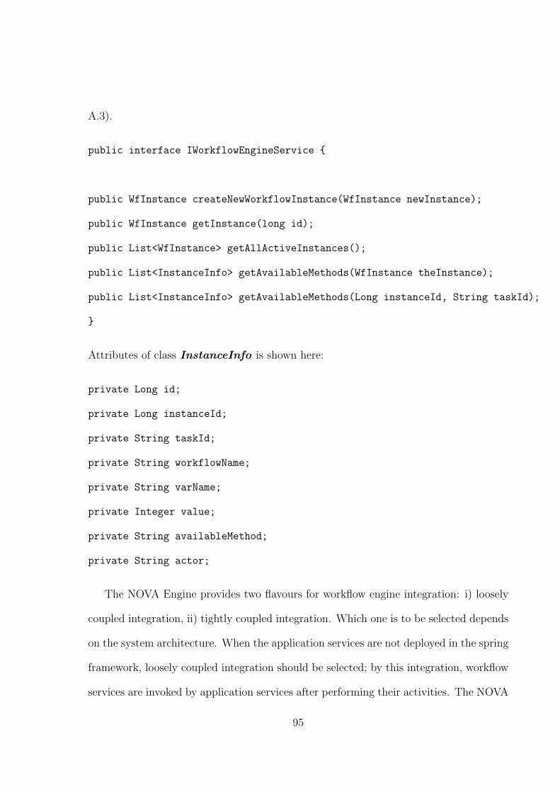
A.3).
public interface IWorkflowEngineService {
public WfInstance createNewWorkflowInstance(WfInstance newInstance);
public WfInstance getInstance(long id);
public List<WfInstance> getAllActiveInstances();
public List<InstanceInfo> getAvailableMethods(WfInstance theInstance);
public List<InstanceInfo> getAvailableMethods(Long instanceId, String taskId);
}
Attributes of class InstanceInfo is shown here:
private Long id;
private Long instanceId;
private String taskId;
private String workflowName;
private String varName;
private Integer value;
private String availableMethod;
private String actor;
The NOVA Engine provides two flavours for workflow engine integration: i) loosely
coupled integration, ii) tightly coupled integration. Which one is to be selected depends
on the system architecture. When the application services are not deployed in the spring
framework, loosely coupled integration should be selected; by this integration, workflow
services are invoked by application services after performing their activities. The NOVA
95

Engine updates the task status when a particular service bean is invoked. On the other
hand, if the application services are deployed in the spring container, tightly coupled
integration is recommended; here application services are extended by workflow service
classes.
7.1.3 The NOVA translator
In [36] we proposed an automatic translator which translates a graphical model con-
structed using the YAWL editor to DVE. The approach was different and it was based
on channels, signals, etc rather than Petri net based. The NOVA Workflow incorporates
an automated translator from CWML to DVE the modeling language of the DiVinE
model checker using methods described in chapter 5. To verify a workflow, a task’s
specifications need to be written in its property file. A task’s property file is a Java class
which extends abstract classes of the NOVA Translator API (see Table A.1 in appendix).
A parser reads a task’s specifications and the translator translates them to DVE. The
NOVA translator has two additional features with which it can handle the state explosion
problem for a complex workflow system: i) Data abstraction, ii) Workflow Reduction.
Data abstraction
It is important to note that not all the attributes of Java entities are important for
model checking; for example, a patient’s name generally does not carry any important
information that can direct a health care workflow. When writing the specifications for
tasks, one should concentrate on the attributes that can directly or indirectly affect the
flow of execution. NOVA WorkFlow provides a Util class which has a method named
getNonDeterministicData(). Using this method the system designer can specify
96

public class Receive_Referral extends UncompensableTaskMCImpl
{
ReferralInfoDTO referralA;
int age;
@Override
public void initialize() {
age = (Integer) Util.getNonDeterministicData(new Integer[]{15,30,45,60});
}
......
}
Figure 7.5: Syntax for assigning non-deterministic data
the data set for a particular variable. For model checking it is expected to use Fuzzy
values which covers sample values from every category of the domain. For example the
property age of a person can have many discrete values. If this is an integer, the domain
is -32768 to +32767; however, if we consider a Banking system, it runs its business based
on 3 or 4 categories of age values, making a different policy for junior, adult and senior.
If a model checking program is allowed to have all possible values from the domain, there
will be huge state explosion which can be drastically reduced by taking only abstract
values for a variable. Data abstraction is an essential and important issue for model
checking. The code snippet in Fig. 7.5 shows an example usage of data abstraction.
The NOVA translator will generate four non-deterministic choices (15,30,45,60) for the
age variable in the DVE translation. Fig. 7.6 shows the translated DVE code of these
non-deterministic values.
97

Figure 7.6: DVE code for non-deterministic data
NOVA Workflow allows you to write abstract task specification using limited number
of Java syntax in a task property file. As this file will be translated to the input language
of a model checker, not all java syntax is supported. The syntax of writing abstract task
specification is provided in the appendix.
Workflow reduction
The NOVA translator incorporates the Reduction algorithm described in chapter 6 which
reads a property to be verified, written in Linear Temporal Logic, the workflow model
and the task’s property (i.e., pre-conditions, actions) and reduces the workflow model by
removing the tasks and properties which do not directly or indirectly affect the execution
flow, before verifying the property. If no LTL-property file is specified it translates the
entire workflow without performing any reduction.
7.1.4 The NOVA browser
The NOVA Browser hierarchically represents database records using a mind map. A
mind map [12] is a graphical way to represent ideas and concepts. A mind map (as
opposed to traditional notes or text) structures information in a way that resembles
much more closely how the brain actually works. Since it is an activity that is both
98

analytical and artistic, it engages the human brain in a much richer way, helping in
all its cognitive functions. Mind maps are used to generate, visualize, structure, and
classify ideas, and as an aid to studying and organizing information, solving problems,
making decisions, and writing. Pictorial methods for recording knowledge and modelling
systems have been used for centuries in learning, brainstorming, memory, visual thinking,
and problem solving by educators, engineers, psychologists, and others. Although these
methods have been used for a long time by analysts and individuals, its use in software
systems to provide a means to involve the user more with the system is rare. The browser
displays all the necessary information for a user in one page. Information (nodes) are
presented into the map radially around the centre node. For example for a HealthCare
application, a physician can select a patient’s case and view all the information related
to the patient in a hierarchical fashion allowing the user to concentrate more on the
patient’s condition and health. Fig. 7.7 shows a patient’s information in hierarchical
fashion in the NOVA Browser.
Time travel view
The browser incorporates a time travel view with which the user can go back in time and
can check previous information. In order to enable the time travel view, the database
tables need some extra columns to preserve the historical information and time. Let us
define the Timed Table here:
Definition 7.1. A Timed Table has the following 5 columns in addition to other custom
columns:
• id: is a primary key,
99
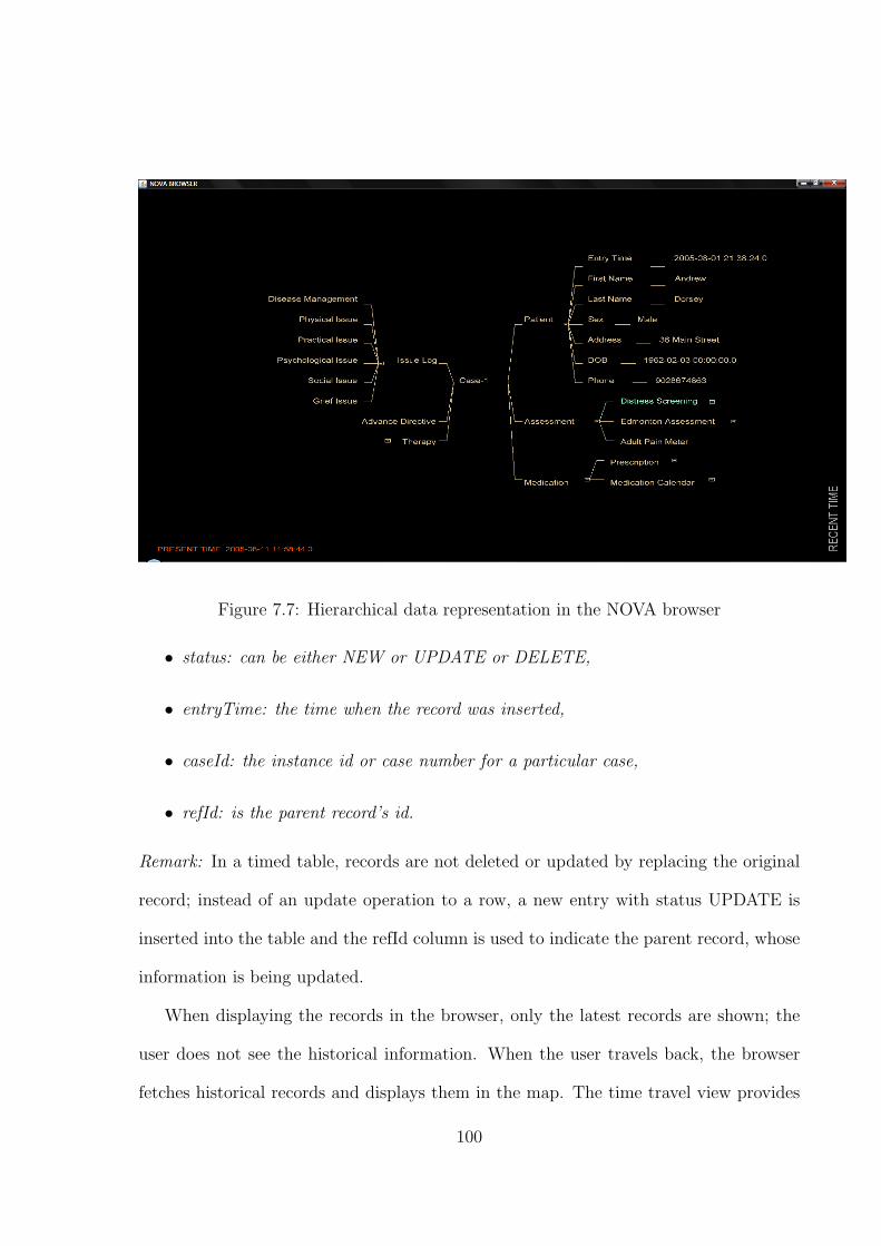
Figure 7.7: Hierarchical data representation in the NOVA browser
• status: can be either NEW or UPDATE or DELETE,
• entryTime: the time when the record was inserted,
• caseId: the instance id or case number for a particular case,
• refId: is the parent record’s id.
Remark: In a timed table, records are not deleted or updated by replacing the original
record; instead of an update operation to a row, a new entry with status UPDATE is
inserted into the table and the refId column is used to indicate the parent record, whose
information is being updated.
When displaying the records in the browser, only the latest records are shown; the
user does not see the historical information. When the user travels back, the browser
fetches historical records and displays them in the map. The time travel view provides
100

an easy way for the user to go back to when a certain record was inserted or updated and
can check its effect by travelling forward from that time. The NOVA Browser provides
four types of time travel:
• Travel back to a past time when a selected record was inserted, updated or deleted;
in this case, the user needs to select a node.
• Travel forward to a future time when a selected record was inserted, updated or
deleted; here the user also needs to select a node.
• Travel one step back to the previous time when any record was inserted or updated
for the selected case; in this case the user does not select a node and the search
operation is performed globally on all tables for the case.
• Travel one step forward to the next time when any record was inserted or updated
for the selected case; here the user does not select a node and thus the search
operation is performed globally on all tables.
If the user selects the ‘Assessment’ node and travels back, the browser will jump to
the time when an Assessment record was inserted or updated. Note that, Assessment
is an abstract base class with four concrete subclasses. NOVA Browser displays the
transition from one mind map to another by doing animation about the Z-axis, giving
the impression of travelling backward and forward.
The Chart view
Charts and graphs play an important role for analyzing information. The visual rep-
resentation of complex information can help researchers process large amounts of data
101

to detect and observe patterns. However it is very difficult to pre-configure all types
of charts with the different combination of parameters that are needed by many appli-
cations. The NOVA Browser incorporates a chart view where the user can select his
chart parameters. The user selects some nodes from the browser and adds them to the
parameter list. The user selects a time range and the chart viewer generates the chart
using those selected parameters by plotting time on the X-axis and the parameters on
the Y-axis. As the user can select any node from the browser, the browser will either
plot the exact value of the parameter or present them symbolically. Table 7.1 shows the
parameter data types and their graphical representation. Fig. 7.8 shows an example of
NOVA Chart where Radiology, Administered Medicine are string parameters, Pain and
Nausea are integer parameters.
Parameter Data Type Rresentation
String String
boolean Symbolic (X,×)
int,float,double Bar chart
date Symbolic (X)
Class Symbolic (X,×)
Table 7.1: Parameter data types and their graphical representations
102
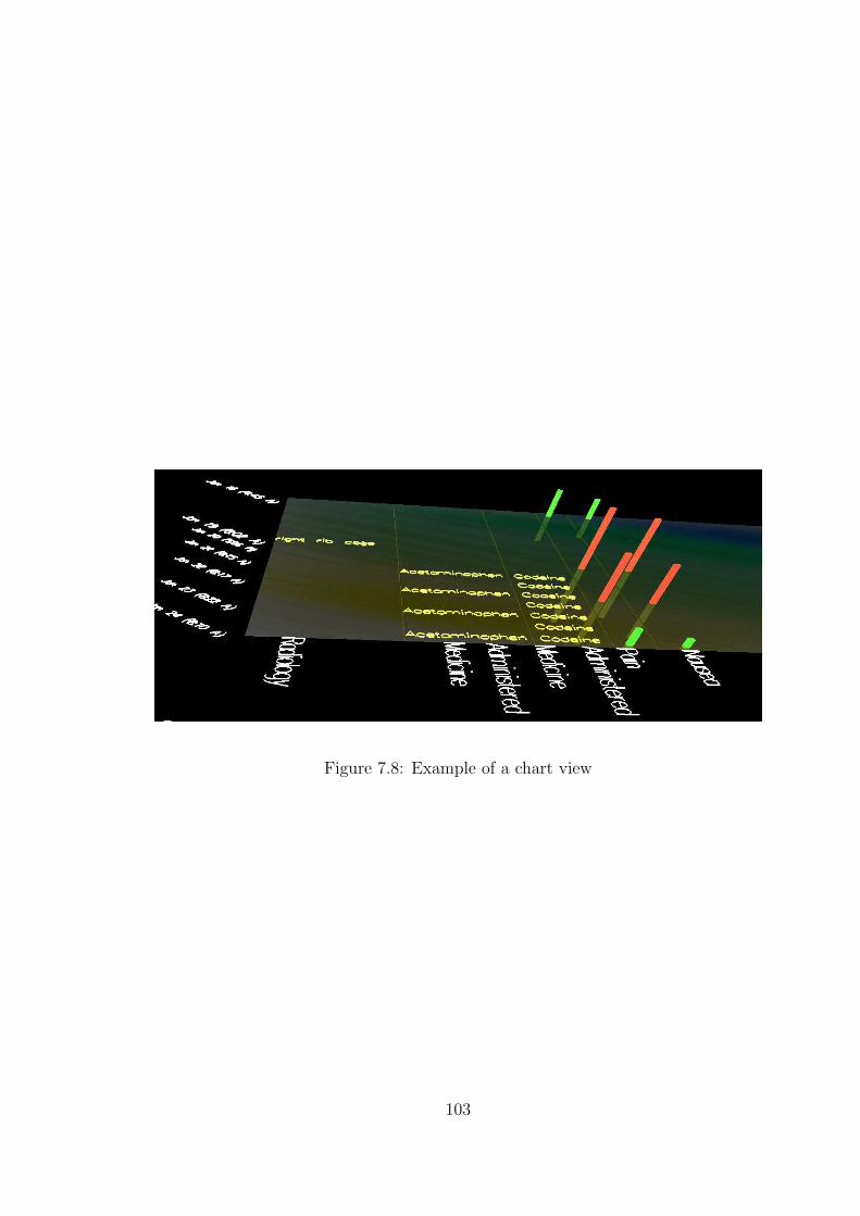
Figure 7.8: Example of a chart view
103

Chapter 8
Case study
In this chapter we will see how NOVA Workflow can be useful in the verification of
properties of a real life workflow. NOVA Workflow was used for modeling and verifying
of a Hospice Palliative Care workflow developed in collaboration with a local health
authority, the Guysborough Antigonish Strait Health Authority (GASHA).
8.1 Hospice palliative care
Palliative Care refers to the medical or comfort care that reduces the severity of a
disease or slows its progress, rather than providing a cure. For incurable diseases, in
cases where the cure is not recommended due to other health concerns, and when the
patient does not wish to pursue a cure, palliative care becomes the focus of treatment.
For example, if surgery cannot be performed to remove a tumor, radiation treatment
might be tried to reduce its rate of growth, and pain management could help the patient
manage physical symptoms. Hospice Palliative Care (HPC) in Canada is guided by
the Canadian Hospice Palliative Care Association (CHPCA) National Model (2002) [16]
104

which espouses a collaborative, patient/family centred approach to care.
Figure 8.1: Overview of CHPCA model
The CHPCA National Model was built on an understanding of health, the illness and
bereavement experiences, and the role hospice palliative care plays in relieving suffering
and improving quality of life. This national model is a tool to guide all activities re-
lated to hospice palliative care. It was developed in consultation with experts across the
country, and based on patient and family issues/needs (as opposed to existing funding
and service delivery models), and created a shared vision and set the stage for a con-
sistent, standardized approach to patient and family care, organizational development,
education and advocacy across the country. It was developed to guide both:
• the process of providing care to patients and families through both the illness and
105

bereavement experiences
• the development and function of hospice palliative care organizations.
The palliative care model has principles to guide data collection and the model is
based on “norms of practice” that support the development of local standards while
supporting the goal of quality care.
Modeling of palliative care process
The process for providing care involves the following six essential and several basic steps
that guide the interaction between caregivers, and the patient and family:
1. Assessment
2. Information Sharing
3. Decision-making
4. Care Planning
5. Care Delivery
6. Confirmation
A palliative care workflow model was designed from CHPCA norms; GASHA forms
were mapped into processes (i.e., using form attributes in task pre-conditions and ac-
tions). Fig. 8.2 shows the high level model of the workflow consisting of composite
tasks. Each of the composite task has a subnet workflow. Some of them are described
in subsequent sections. Fig. 8.3 shows a GASHA form to record pain level.
106
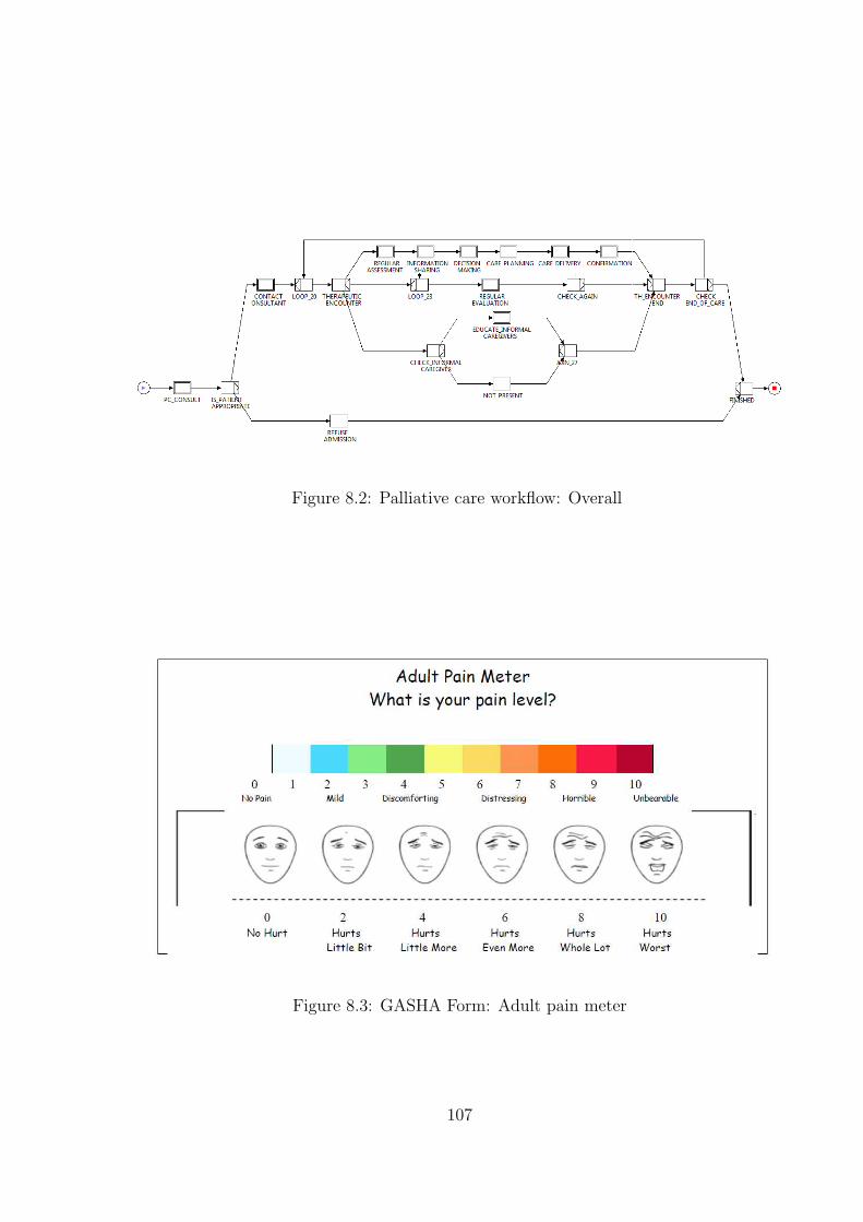
Figure 8.2: Palliative care workflow: Overall
Figure 8.3: GASHA Form: Adult pain meter
107

Overall model
A patient is referred to the palliative care program from ‘Continuing care’ or ‘Consult
team’. When a patient referral is received, it is determined in the PC Consult subnet
whether the patient is eligible for Hospice Palliative Care. If the patient is not eligible,
the workflow will end with a proper explanation. Otherwise the patient is sent for the
next set of care tasks. The patient consults with a physician and the registration is
performed. During each therapeutic encounter the workflow ensures that the basic steps
are covered. Thus assessments, care planning, etc. occur regularly. The Information
Sharing step identifies the confidentiality limits: what the patient and family already
know, what they would like to know, and whether they are ready to listen is established
before sharing information. If language is a barrier, translators who understand the
medical concepts and terminology will be employed to facilitate information sharing.
The patient’s and family’s desire for additional information is assessed regularly. In
the Decision Making step the patient’s decision-making capacity, and the patient’s and
family’s goals are assessed regularly. In this step, the patient and family will prioritize
the importance of each of the identified issues. In addition, requests to withhold or
withdraw therapies, and requests to initiate therapeutic interventions that appear to
have no potential to benefit the patient and family, and the factors underlying those
requests, are discussed openly. Therapies, therapeutic options and patient and family
choices are reviewed. After the Decision Making comes the Care Planning step. The
plan of care includes strategies for addressing each of the patient’s and family’s issues or
opportunities, expectations, needs, hopes and fears, for delivering their chosen therapies,
providing backup coverage if care givers are unable to fill their role in the plan of care,
and for providing care giver respite, coping with emergencies, planning for discharge,
108

and etc. In this step, patients and families are assisted by the care team coordinators
to select an appropriate setting of care. The plan and setting of care are reviewed by
the care team and/or the organization’s regional team and adjusted to compensate for
changes in the patient’s and family’s status and choices. When it comes to the Care
Delivery step, care is provided by a specific interdisciplinary care team that forms to care
for each patient/family unit. Each care team has the leadership it needs to facilitate care
team formation and function, and coordinate care planning and delivery. The setting
of care is maintained so that it is safe, comforting, and provides ample opportunity
for privacy and intimacy. The compatibility of the medicines is checked in this step.
Any errors in therapy delivery are reported to supervisors immediately and documented
appropriately. ‘Regular Evaluation’ is conducted regularly by the formal caregivers to
assess and reinforce the patient’s, family’s and informal care giver’s understanding of
the situations such as the plan of care, the appropriate use of medications, therapies,
equipment and supplies.
Registration
Fig. 8.4 shows the registration subnet. A nurse consultant collects the information from
patient and makes a patient file. During the execution of the ‘Fill Patient Info Form’
process two important data (i.e., patient’s location and PPS value) are collected which
are used in many places of the workflow to make decisions. In the task property file (i.e.,
‘Fill Patient Info Form.java’) these two attributes are set with possible non-deterministic
values. The syntax for writing the abstract specification is provided here:
public class Fill_Patient_Info_Form extends UncompensableTaskMCImpl
{
109

Patient thePatient;
Patient.Location patientsLocation;
PatientData patientData;
Integer ppsValue;
@Override
public void action() {
// TODO Auto-generated method stub
}
@Override
public void finalize() {
thePatient.setPatientLocation(patientsLocation);
patientData.setpPS(ppsValue);
}
@Override
public void initialize() {
patientsLocation = (Patient.Location)Util.getNonDeterministicData(
new Patient.Location[]{Patient.Location.HOME, Patient.Location.HOSPITAL});
ppsValue = (Integer) Util.getNonDeterministicData(new Integer[]{40,50,60});
}
}
Intake
Patients issues are identified from the process ‘Identify Issues’ and some data (e.g.,
preferred language, advanced directives, consent to contact other team members) are
110

Figure 8.4: Registration
collected from this process. The patients’ medication history is collected and distress
screening is measured. Fig. 8.5 shows the subnet workflow.
Figure 8.5: Palliative care workflow: Intake
Regular assessment
During each therapeutic encounter, the patient’s condition is assessed by various per-
formance metrices and tests in the ‘Regular Assessment’ subnet. Fig. 8.6 shows the
‘Regular Assessment’ subnet of the palliative care workflow which consists of ‘Adult
111

pain meter’, ‘Edmonton assessment’, ‘Palliative performance scale’, ‘Distress screening’
processes.
Figure 8.6: Palliative care workflow: Regular Assessment
Team building
A care team is built for a palliative care patient consisting of formal and informal care
givers. We modeled the ‘Team Building’ subnet (Fig. 8.7) with compensable tasks. If the
patient’s location is at home, then a home service is assigned; but if there is no home
service available for the given location, the patient must move to the hospital. This flow
is designed with an ‘Alternative Choice’ composition. The code snippet to check the
patient’s location for the task ‘Check Patient Location’ is given below:
public class Check_Patient_Location extends InternalChoiceSplitMCImpl
112

{
Patient thePatient;
Patient.Location location;
.......
@Override
public void initialize() {
location = thePatient.getPatientLocation();
}
@Override
public boolean branchCondition(int branchNo) {
if(branchNo == 1)
return location == Patient.Location.HOME;
else
return location == Patient.Location.HOSPITAL;
}
}
To assign a formal caregiver for the patient an speculative choice block was designed.
A family physician or a pc physician, whoever comes first, is assigned to the patient.
8.2 Verification of the palliative care process
Norms from the CHPCA National Model are general statements of guidelines. Some
of the properties we verified are listed below, along with the CHPCA norms that they
113

Figure 8.7: Palliative care workflow: Team Building
114

pertain to:
Prop1 (N5.1, N1.1)- If patient is distressed, then a Social Worker must be assigned in
the care team.
#define patient_is_distressed (patientsDistressScreening_distressed == 1 )
#define patient_is_not_distressed (patientsDistressScreening_distressed == 0)
#define social_worker_is_assigned (careTeam_socialWorker_ELEMENT_0_id > 0 )
#define end_of_care_reached patientData_isEndOfCare == 1
#define composition_ok _Workflow_Composition_Ok == 1
#property ( G composition_ok) -> G ( patient_is_distressed ->
F ( patient_is_not_distressed || end_of_care_reached ||
social_worker_is_assigned ) )
Prop2 (N1.2)- If the patient does not have anyone designated as their Next of Kin, then
the “Interview With Family Member” task will not execute.
#define nextofkin_not_present (thePatient_nextOfKin_id == 0)
#define interview_done (assessment_interviewWithFamilyMember > 0 )
#define composition_ok _Workflow_Composition_Ok == 1
#property ( G composition_ok) -> G ( nextofkin_not_present ->
F interview_done )
Prop3 (N3.5, N4.1, N4.4, N5.3)- If the patient is at home and has no family, then there
must be an Informal Caregiver provided. Otherwise, the patient must be moved to the
hospital.
115

#define patient_at_home thePatient_patientLocation == 0
#define patient_at_hospital thePatient_patientLocation == 1
#define home_service_assigned careTeam_homeServiceCaregivers_ELEMENT_0_id > 0
#define informal_cg_assigned careTeam_familymemberCaregivers_ELEMENT_0_id > 0
#define composition_ok _Workflow_Composition_Ok == 1
#property ( G composition_ok) -> G ( patient_at_home -> F (home_service_assigned
|| informal_cg_assigned || patient_at_hospital ) )
Prop4 (N1.2)- If there is a risk for staff who visit the patient’s home, then there will be
no formal care provided to the patient in their home. They must come to the hospital.
#define patient_at_home thePatient_patientLocation == 0
#define patient_at_hospital thePatient_patientLocation == 1
#define there_is_a_risk preVisitRiskAssessment_isThereARisk_yesOrNo == 1
#define composition_ok _Workflow_Composition_Ok == 1
#property ( G composition_ok) -> G( there_is_a_risk -> F patient_at_hospital )
Prop5 (N3.5, N4.1, N4.4)- If the patient is evaluated and assigned a PPS of 50% or
lower, then they must be moved to the hospital.
#define pps_lower_than_50 patientData_pPS <= 50
#define patient_at_hospital thePatient_patientLocation == 1
#define composition_ok _Workflow_Composition_Ok == 1
116

#property ( G composition_ok) -> G ( pps_lower_than_50 -> F patient_at_hospital )
Prop6 (N3.5, N4.1, N4.4)- If the patient is evaluated and assigned a level of 3 or lower,
then they must be moved to the hospital.
#define patient_at_level_three_or_lower patientData_level <= 3
#define patient_at_hospital thePatient_patientLocation == 1
#define composition_ok _Workflow_Composition_Ok == 1
#property ( G composition_ok) -> G ( patient_at_level_three_or_lower ->
F patient_at_hospital )
Prop7 (N3.7, N3.8, N3.9)- If the patient is no longer capable of making decisions, then
there must be a proxy decision maker assigned.
#define patient_is_not_capable patientData_isCapable == 0
#define proxy_is_a_kin patientsAdvanceDirectives_proxy_id == 1
#define proxy_is_not_a_kin patientsAdvanceDirectives_proxy_id == 2
#define proxy_is_not_made patientsAdvanceDirectives_proxy_id == 0
#define composition_ok _Workflow_Composition_Ok == 1
#property ( G composition_ok) -> G ( patient_is_not_capable ->
F ( proxy_is_a_kin || proxy_is_not_a_kin ))
Prop8 (N2.4)- If the patient needs a translation of the information provided to him/her,
then the translation will be provided.
#define translation_required patientsIssueLog_log1_preferredLanguage != 0
117

#define translation_is_done patientsIssueLog_log1_isTranslationDone == 1
#property G (translation_required -> F translation_is_done )
Prop9 (N5.1, N1.1, N1.3)- If patients mobility is changed, then a Physiotherapist will
be notified.
#define change_in_mobility theCommunicationSheet_changeInMobility == 1
#define physiotherapist_assigned (careTeam_physiotherapist_ELEMENT_0_id > 0 )
#define composition_ok _Workflow_Composition_Ok == 1
#property ( G composition_ok) -> G ( change_in_mobility ->
F physiotherapist_assigned )
Prop10 (N2.1)- If the field “Consent to Contact Other Team Member” on ‘Issues Log’
is set to YES, then Consent to Share Information must be filled out.
#define advance_directive_is_required patientsIssueLog_advancedDirectives == 1
#define advance_directive_is_filled_out (patientsAdvanceDirective_id > 0 )
#property G ( advance_directive_is_required ->
F advance_directive_is_filled_out )
Note that Java entity class references and their attributes are translated to DiVinE data
type and variables. To write a LTL-property the translated DiVinE variable names are
used. The DVE code for Prop1 is shown here:
118

Property Acc Cycle WR + POR POR
States Memory Time States Memory Time
(MB) (s) (MB) (s)
Prop1 No 107167421 83315.3 305.3 Unknown Overflow > 1hour
Prop2 No 24501 220.0 7.9 Unknown Overflow > 1hour
Prop3 No 126188210 88619.1 384.3 236576621 143836.2 1860
Prop4 No 13443 285.3 5.0 Unknown Overflow > 1hour
Prop5 No 128013744 88920.0 397.9 251323543 153290.3 1931
Prop6 No 127934841 88894.5 396.1 213254702 140215.0 1854
Prop7 No 21234 274.5 6.1 Unknown Overflow > 1hour
Prop8 No 12190 4.5 4.1 Unknown Overflow > 1hour
Prop9 No 132038485 90285.3 315.0 211347231 139521.1 1833
Prop10 No 13479 230.1 9.7 202233451 125804.1 1803
Table 8.1: Verification results for the DiVinE model checker
All experiments were executed on the Mahone2 cluster of ACEnet, the high per-
formance computing consortium for universities in Atlantic Canada. The tests were
performed using DiVinE with 64 CPU’s and 3GB memory (per CPU). After several
iterations of modeling and verification the properties were verified; the results are shown
in Table 8.1.
119

Chapter 9
Conclusion and future work
Model checking has been successfully applied to verify hardware systems (e.g., embed-
ded system, circuits, communication protocols). It has a number of advantages over
traditional approaches of validation/verification that are based on simulation, testing
and deductive reasoning. This is a popular technique as it performs the verification pro-
cess automatically and produces a counter-example that is useful in debugging a system.
However, software systems are generally much more complex than hardware systems.
To verify a software system using the model checking approach needs a great deal of
research as model checking often suffers from the state explosion problem. Building the
abstract finite state machine from the given software design and verifying the abstract
finite state machine might solve the state explosion problem but it requires a lot of time
and effort for modeling which is offen error prone. In this thesis we have presented a tool
NOVA Workflow to design a workflow model that supports verification. With it one can
graphically design a workflow and write business logic for the tasks. On the other hand
abstract specifications (e.g., pre-conditions, actions, abstract values for variables, etc.)
for tasks can be written in the task property file which is subject to the verification. The
120

workflow model is then automatically translated to a model checking program. This will
significantly reduce the time and effort required to build an abstract state machine from
an enterprise software system. Beside this we have presented a reduction algorithm that
reduces the number of concurrent tasks from a workflow model and produces a small
workflow model preserving required properties of the system. We have shown the appli-
cability of this tool on a fairly big model for a health-care application. Our case study
shows the effectiveness of the tool.
The specific contributions of this thesis are listed here:
• Proof of associativity for t-Calculus operatos (||,⊓, and ⊗) in section 3.2.9.
• A graphical compensable workflow modeling language based on t-Calculus opera-
tors:
– Definition of atomic task, nonatomic task and compensable task: Definition
4.1 - 4.5;
– Definition of Compensable Workflow Net in Definition 4.6;
– Graphical workflow modeling language in Fig. 4.3 and its Petri net represen-
tation in section 4.2;
– Soundness analysis of CWML in section 4.3;
• Automated translation of a workflow model to a model checker DiVinE, along with
the proof of correctness:
– Translation algorithm in Algorithm 1;
– Proof of correctness in section 5.2.2;
• A Workflow Reduction method and its proof of stuttering equivalence:
121

– Wofkflow reduction algorithm in Algorithm 3;
– Proof of stuttering equivalence in section 6.3;
– Effectiveness of the reduction studied in section 6.4;
• A workflow management system named NOVA Workflow to design, develop, verify
and analyse compensable workflows discussed in (chapter 7). The software may
be found in [7].
• Modeling and verification of a palliative care system as a case study, (chapter 8).
In future we will incorporate a sophisticated ontology to guide the workflow and
explicit-time description methods [47] [30] into workflow modeling and verify larger mod-
els of real-world health-care processes with timing information. We will also incorporate
a personalized health-care access control system into the NOVA Workflow.
122

Bibliography
[1] Divine project, http://divine.fi.muni.cz/. last accessed on nov: 2010.
[2] Eclipse plugin. http://www.eclipse.org/articles/article-plug-in-
architecture/plugin architecture.html/. last accessed, August 2010.
[3] Graphical editing framework. http://www.eclipse.org/gef/. last accessed, August
2010.
[4] Relational persistence for java and .net, http://hibernate.net/. last accessed,
November 2010.
[5] Spring framework, http://www.springsource.org/. last accessed, November 2010.
[6] Bpel2pn. http://www2.informatik.hu-berlin.de/top/bpel2pn/. last accessed, Febru-
ary 2011.
[7] Nova workflow. http://logic.stfx.ca/software/nova-workflow/. last accessed, March
2011.
[8] Wsengineer. http://www.doc.ic.ac.uk/ltsa/eclipse/wsengineer/. last accessed,
February 2011.
123

[9] Assaf Arkin and Intalio. Business process modeling language. BPML specification,
November 2002.
[10] Ahmed Awad, Gero Decker, and Mathias Weske. Efficient compliance checking
using bpmn-q and temporal logic. In Proceedings of the 6th International Conference
on Business Process Management, BPM ’08, pages 326–341, Berlin, Heidelberg,
2008. Springer-Verlag.
[11] Jiri Barnat, Lubos Brim, and Petr Rockai. Scalable multi-core ltl model-checking.
In SPIN, pages 187–203, 2007.
[12] Tony Buzan. The Mind Map Book. Penguin Books, 1996.
[13] E. Clarke, O. Grumberg, and D. Long. Model checking. In Proceedings of the NATO
Advanced Study Institute on Deductive program design, pages 305–349, Secaucus,
NJ, USA, 1996. Springer-Verlag New York, Inc.
[14] Edmund M. Clarke and E. Allen Emerson. Design and synthesis of synchronization
skeletons using branching-time temporal logic. In Logic of Programs, pages 52–71,
1981.
[15] Edmund M. Clarke, E. Allen Emerson, and A. Prasad Sistla. Automatic verification
of finite-state concurrent systems using temporal logic specifications. ACM Trans.
Program. Lang. Syst., 8(2):244–263, 1986.
[16] Frank D. Ferris, Heather M. Balfour, Karen Bowen, Justine Farley, Marsha Hard-
wick, Claude Lamontagne, Marilyn Lundy, Ann Syme, and Pamela J. West. A
model to guide hospice palliative care. Canadian Hospice Palliative Care Associa-
tion, 2002.
124

[17] Hector Garcia-Molina and Kenneth Salem. Sagas. SIGMOD Rec., 16:249–259,
December 1987.
[18] Jifeng He. Modelling coordination and compensation. In ISoLA, pages 15–36, 2008.
[19] David Hollingsworth. The workflow reference model. Workflow Management Coali-
tion, January 1995.
[20] Microsoft SAP Siebel IBM, Bea. Business process execution language for web ser-
vices version 1.1. May 2003.
[21] He Jifeng. Formal methods and hybrid real-time systems. chapter Compensable
programs, pages 349–363. Springer-Verlag, Berlin, Heidelberg, 2007.
[22] Edmund M. Clarke Jr., Orna Grumberg, and Doron A. Peled. Model Checking. The
MIT Press, 1999.
[23] Saul Aaron Kripke. A semantical analysis of modal logic I: Normal modal proposi-
tional calculi. Zeitschrift fur Mathematische Logik und Grundlagen der Mathematik,
9:67–96, 1963.
[24] Gary T. Leavens, K. Rustan M. Leino, and Peter Muller. Specification and veri-
fication challenges for sequential object-oriented programs. Form. Asp. Comput.,
19:159–189, June 2007.
[25] Nazia Leyla, Ahmed Mashiyat, Hao Wang, and Wendy MacCaull. Workflow Veri-
fication with DiVinE. In Parallel and Distributed Methods in verifiCation. PDMC,
2009.
125

[26] Jing Li, Huibiao Zhu, and Jifeng He. Algebraic semantics for compensable transac-
tions. In Proceedings of the 4th international conference on Theoretical aspects of
computing, ICTAC’07, pages 306–321, Berlin, Heidelberg, 2007. Springer-Verlag.
[27] Jing Li, Huibiao Zhu, and Jifeng He. Specifying and verifying web transactions. In
Formal Techniques for Networked and Distributed Systems - FORTE 2008, volume
5048 of Lecture Notes in Computer Science, pages 149–168. Springer-Verlag, 2008.
[28] Jing Li, Huibiao Zhu, Geguang Pu, and Jifeng He. A formal model for compensable
transactions. In Proceedings of the 12th IEEE International Conference on Engi-
neering Complex Computer Systems, pages 64–73, Washington, DC, USA, 2007.
IEEE Computer Society.
[29] Jing Li, Huibiao Zhu, Geguang Pu, and Jifeng He. Looking into compensable trans-
actions. Software Engineering Workshop, Annual IEEE/NASA Goddard, 0:154–166,
2007.
[30] Ahmed Shah Mashiyat, Fazle Rabbi, Hao Wang, and Wendy MacCaull. An auto-
mated translator for model checking time constrained workflow systems. In FMICS,
pages 99–114, 2010.
[31] Jan Mendling. On the detection and prediction of errors in epc business process
models. EMISA Forum, 27(2):52–59, 2007.
[32] Tadao Murata. Petri nets: properties, analysis, and applications. Proceedings of
the IEEE, 77(4):541–580, 1989.
[33] Carl Adam Petri. Kommunikation mit automaten. PhD thesis, Institut fur instru-
mentelle Mathematik, Bonn, 1962.
126

[34] Amir Pnueli. The temporal logic of programs. In FOCS, pages 46–57, 1977.
[35] Jean-Pierre Queille and Joseph Sifakis. Specification and verification of concurrent
systems in cesar. In Proceedings of the 5th Colloquium on International Symposium
on Programming, pages 337–351, London, UK, 1982. Springer-Verlag.
[36] Fazle Rabbi, Hao Wang, and Wendy MacCaull. Yawl2dve: An automated translator
for workflow verification. In Secure Software Integration and Reliability Improve-
ment, pages 53–59, 2010.
[37] M.U. Reichert, S.B. Rinderle, U. Kreher, H. Acker, M. Lauer, and P. Dadam.
Adept2 - next generation process management technology. In Proceedings Fourth
Heidelberg Innovation Forum, Aachen, April 2007. D.punkt Verlag.
[38] Wasim Sadiq and Maria E. Orlowska. Applying graph reduction techniques for
identifying structural conflicts in process models. In Proceedings of the 11th In-
ternational Conference on Advanced Information Systems Engineering, CAiSE ’99,
pages 195–209, London, UK, 1999. Springer-Verlag.
[39] Wasim Sadiq and Maria E. Orlowska. Analyzing process models using graph reduc-
tion techniques. Inf. Syst., 25(2):117–134, 2000.
[40] W. M. P. van der Aalst and Ter. YAWL: yet another workflow language. Information
Systems, 30(4):245–275, June 2005.
[41] Wil M. P. van der Aalst. The application of petri nets to workflow management.
Journal of Circuits, Systems, and Computers, 8(1):21–66, 1998.
127

[42] Wil M. P. van der Aalst. Business process management demystified: A tutorial on
models, systems and standards for workflow management. In Lectures on Concur-
rency and Petri Nets, pages 1–65, 2003.
[43] Wil M. P. van der Aalst and Kees van Hee. Workflow Management: Models, Meth-
ods, and Systems. MIT Press, 2002.
[44] Wil M. P. van der Aalst, Kees M. van Hee, Arthur H. M. ter Hofstede, Natalia
Sidorova, H. M. W. Verbeek, Marc Voorhoeve, and Moe Thandar Wynn. Soundness
of workflow nets with reset arcs. T. Petri Nets and Other Models of Concurrency,
3:50–70, 2009.
[45] Boudewijn F. van Dongen, Wil M. P. van der Aalst, and H. M. W. Verbeek. Ver-
ification of epcs: Using reduction rules and petri nets. In CAiSE, pages 372–386,
2005.
[46] Martin Vasko and Schahram Dustdar. A view based analysis of workflow modeling
languages. In Proceedings of the 14th Euromicro International Conference on Par-
allel, Distributed, and Network-Based Processing, pages 293–300, Washington, DC,
USA, 2006. IEEE Computer Society.
[47] Hao Wang and Wendy MacCaull. An efficient explicit-time description method for
timed model checking. In PDMC, pages 77–91, 2009.
128

Appendix A
A.1 Syntax for writing abstract tast specification
A.1.1 Supported data types
To write an abstract task specification for verification you can only use byte, integer, long
and boolean, although these data types can be specified inside a Class, List, Vector or
Aggregate Class. String, Float and Double are not supported as they are not supported
by the model checker. NOVA workflow handles ‘entity class references’ and ‘variables
with primitive data type’ in two different ways; entity class references are translated to
the ‘Global variables’ in DVE and variables with primitive data types are translated to
‘Local variables’. While writing the specification, the entity class references can be used
for interprocess communication.
A.1.2 Details of task property files
Abstract task specifications are written in task property files those are Java classes.
NOVA workflow provides different interfaces for writing task specification. Table A.1
shows the list of task types and their interfaces and methods. To initialize a local
variable (primitive data type) with non-deterministic values or from any global variable
129

(entity class reference) the initialize() method is used. Statements with assignment or
arithmatic operations can be written in the action() method. Boolean expressions can be
written inside the branchCondition() method; this method is used to write the condition
for different branches of a split task. Finalize() method can be used to set something
into a global variable (entity class reference). Table A.2 lists allowed syntax for different
methods.
Task Type Interface Abstract Methods
AtomicTask UncompensableTaskMCImpl initialize(), action(), finalize()
AndSplitTask AndSplitMCImpl initialize(), action(), finalize()
AndJoinTask AndJoinMCImpl initialize(), action(), finalize()
XorSplitTask XorSplitMCImpl, initialize(), action(), finalize(),
IMCBranchCondition, branchCondition(),
IMCBranchOrder getBranchOrder()
XorJoinTask XorJoinMCImpl initialize(), action(), finalize()
OrSplitTask ORSplitMCImpl, initialize(), action(), finalize(),
IMCBranchCondition branchCondition()
OrJoinTask ORJoinMCImpl initialize(), action(), finalize()
LoopSplitTask LoopSplitMCImpl, initialize(), action(), finalize(),
IMCBranchCondition, branchCondition(),
IMCBranchOrder getBranchOrder()
LoopJoinTask LoopJoinMCImpl initialize(), action(), finalize()
Table A.1: Task types and interfaces
130

Task Type Interface Abstract Methods
CompensableTask CompensableTaskMCImpl initialize(), action(), finalize(),
abortInitialize(), abort(), abortFinalize()
ParallelSplitTask ParallelSplitMCImpl initialize(), action(), finalize(),
abortInitialize(), abort(), abortFinalize()
ParallelJoinTask ParallelJoinMCImpl initialize(), action(), finalize(),
abortInitialize(), abort(), abortFinalize()
InternalChoieSplitTask IntrnlChoiceSplitMCImpl, initialize(), action(), finalize(),
IMCBranchCondition abortInitialize(), abort(), abortFinalize(),
branchCondition()
InternalChoiceJoinTask IntrnlChoiceJoinMCImpl initialize(), action(), finalize(),
abortInitialize(), abort(), abortFinalize()
SpeculativeSplitTask SpecChoiceSplitMCImpl initialize(), action(), finalize(),
abortInitialize(), abort(), abortFinalize()
SpeculativeJoinTask SpecChoiceJoinMCImpl initialize(), action(), finalize(),
abortInitialize(), abort(), abortFinalize()
AlternativeSplitTask AltSplitMCImpl, initialize(), action(), finalize(),
IMCBranchOrder abortInitialize(), abort(), abortFinalize(),
getBranchOrder()
Table A.1: Task types and interfaces (Continued)
131

Task Type Interface Abstract Methods
AlternativeJoinTask AltJoinMCImpl initialize(), action(), finalize(),
abortInitialize(), abort(), abortFinalize()
BackwardHandlerTask BckHandlerMCImpl initialize(), action(), finalize()
ForwardHandlerTask FwdHandlerMCImpl initialize(), action(), finalize(),
abortInitialize(), abort(), abortFinalize()
Programmable ProgCmpMCImpl initialize(), action(), finalize()
CompensationTask
Table A.1: Task types and interfaces (Continued)
Method Name Allowed Syntax
initialize(), localVar = (Integer)Util.getNonDeterministicData(new Integer[]1,2,..);
abortInitialize() localVar = (Long)Util.getNonDeterministicData(new Long[]1,2,..);
localVar = (Byte)Util.getNonDeterministicData(new byte[]1,2,..);
localVar = (Boolean)Util.getNonDeterministicData(new Booelan[]true,false);
localVar = globalVar.getAttribute();
localVar = globalVar.getAggregateProperty().getAttribute();
localVar = globalVar.getListAttribute().get(index);
localVar = globalVar.getListAttribute().get(index).getAttribute();
Table A.2: List of allowed syntax in task property file
132
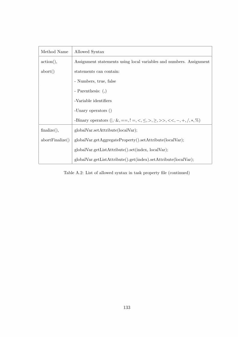
Method Name Allowed Syntax
action(), Assignment statements using local variables and numbers. Assignment
abort() statements can contain:
- Numbers, true, false
- Parenthesis: (,)
-Variable identifiers
-Unary operators ()
-Binary operators (|,,&,==, ! =, <,≤, >,≥, >>,<<,−,+, /, ∗,%)
finalize(), globalVar.setAttribute(localVar);
abortFinalize() globalVar.getAggregateProperty().setAttribute(localVar);
globalVar.getListAttribute().set(index, localVar);
globalVar.getListAttribute().get(index).setAttribute(localVar);
Table A.2: List of allowed syntax in task property file (continued)
133

Method Name Allowed Syntax
branchCondition if(branchNumber == 1) return Boolean Expression;
(int branchNumber) else if(branchNumber == 2) return Boolean Expression;
else return Boolean Expression;
Boolean expressions can be written using local variables and numbers.
The statements can contain:
-Numbers, true, false
-Parenthesis: (,)
-Variable identifiers
-Unary operators ()
-Binary operators (|,,&,==, ! =, <,≤, >,≥, >>,<<,−,+, /, ∗,%)
getBranchOrder if(branchNumber == 1) return 2;
(int branchNumber) else if(branchNumber == 2) return 1;
Table A.2: List of allowed syntax in task property file (continued)
134

A.2 Workflow engine service
Method Name Functionality
createNewWorkflowInstance This method is used to create a new workflow instance.
It inserts a new record in table WfInstance and generates
a unique id for the newly created instance.
getInstance To know details about an instance this method can be used.
getAllActiveInstances This method returns all Active instances
getAvailableMethods There are two overload methods:
i) Takes a workflow instance as parameterand returns all
InstanceInfo containing taskId and available
methods of all active tasks
ii)Takes an instanceId and taskId as parameter and returns
all available methods for the task
Table A.3: Description of the methods of IWorkflowEngineService
135