design development and modeling of a compact field …
TRANSCRIPT
DESIGN, DEVELOPMENT, AND MODELING OF A COMPACT, FIELD-GRADE CIVIL INFRASTRUCTURE CRACK DETECTOR DEVICE
By
© 2014
Alisha M. Elmore
Submitted to the graduate degree program in Civil, Environmental, and Architectural Engineering and the Graduate Faculty of the University of Kansas in partial fulfillment of
the requirements for the degree of Doctor of Philosophy.
________________________________
Chairperson Dr. Stanley T. Rolfe
________________________________
Co-Chairperson Dr. Ronald M. Barrett
________________________________
Dr. Jian Li
________________________________
Dr. Manuel A. Diaz
________________________________
Dr. Steven D. Schrock
Date Defended: July 14, 2014

The Dissertation Committee for Alisha M. Elmore
certifies that this is the approved version of the following dissertation:
DESIGN, DEVELOPMENT, AND MODELING OF A COMPACT, FIELD-GRADE CIVIL INFRASTRUCTURE CRACK DETECTOR DEVICE
________________________________
Co-Chairperson Dr. Stanley T. Rolfe
________________________________
Co-Chairperson Dr. Ronald M. Barrett
Date Approved: August 28, 2014
ii

ABSTRACT
Currently the nation’s aging bridge infrastructure is approaching and in some cases exceeding
its initial design life averaging more than forty years. Under these conditions steel bridges are
susceptible to fatigue cracks at stress ranges below their material yield strength. In order to
evaluate the remaining service life of these structures under their current operating conditions, it
is important to accurately locate and identify active cracks within the material. Early detection of
cracks and defects within a structure can provide inspectors and bridge maintenance personnel
with viable information that can be used in the design and selection of an appropriate retrofit or
repair technique that can be used to extend the service life of the bridge structure. Bridge
inspections are typically conducted every two years primarily using visual inspection techniques.
The active crack sensing tool designed and analyzed in this study is based on the robust and
high sensing capabilities of piezoceramic materials. This dissertation presents the analytical,
computational, and experimental results of a novel approach to identifying and characterizing
cracks in steel bridge structural components using a piezoceramic sensor. Using the newly
designed Piezoelectric Active Crack Tip Sensor (PACTS) tool, it was possible to detect an
active crack with an opening displacement of 0.056 mm [0.0022 in] could be sensed under
dynamic loading conditions. By using a crack opening linear trend (COLT) analysis, the crack
tip position could be located within 3 mm [1/8 in] without the use of correction or modification
factors. The results of the research provide a foundation in establishing an inspection tool
capable of identifying damage detection within an in-service structure. The identification of an
active crack and the ability to locate the crack tip of a material provides bridge inspectors and
maintenance personnel with valuable information related to the current bridge condition that
could be used for maintenance, repair, or replacement of bridges structures in an effort to
ensure the safe passage of people and goods across the nation.
iii

ACKNOWLEDGEMENTS
First and foremost, I would like to give all honor and glory to God our savior. Through him all things are possible. This dissertation would not have been possible without the time, energy, and support of so many people. I was fortunate to be in the right place at the right time to engage in this research study.
I am forever indebted to my committee chairs, Dr. Stanley Rolfe and Dr. Ron Barrett. Both of you took a chance on a new idea and encouraged me to pursue a research topic that was close to my heart and in-line with my future career goals and objectives. I am especially grateful to Dr. Stanley Rolfe for the financial support of me and my project. I would like to thank him for being an amazing and supportive professor, researcher, and advisor. His belief in me and my idea provided me with the strength to stay the course. Dr. Barrett, I doubt I have the words to fully express my appreciation for your technical expertise and your unwavering support. Your ability to facilitate interdisciplinary research and your appreciation for innovation and new technology reminded me why I entered a PhD program. Thank you for re-establishing my belief in research and its potential for real world development and application.
I would also like to thank my committee members Dr. Jian Li and Dr. Steven Schrock for allowing me think outside of the box and for providing me with clarification and technical advice throughout this project. Dr. Li, as a new member of the structures faculty your area of interest in SHM encouraged me to investigate and expand my research project. For his optimism, energy, and support of my academic career, I would like to extend my appreciation and thanks to Dr. Steven Schrock. Thank you for making me laugh, when I was on the verge of tears, and for your generosity in supporting my quest for knowledge.
Special thanks to my long distance committee member Dr. Manuel Diaz for his time, energy, guidance, and overall kindness during my graduate studies. You encouraged me to take this journey and I was fortunate to have you and your family along for the ride. Thank you for keeping me grounded in the real world during my theoretical adventures here at KU.
There are several KU students and faculty that helped make this research possible, whether by means of encouragement or discouragement. Both methods drove me to succeed and steadied my resolve.
I would like to thank the CEAE laboratory staff, Matt Maksimowicz, Eric Nicholson, and David Woody. Thank you for your willingness to help me in all of my destructive laboratory needs. Your eagerness to help me create things so that we could break them, always made me smile.
I would also like to take this opportunity to thank Dr. Glenn Light, Alan Puchot, and members of their NDE Technology Department group for allowing me to tour their facility and helping me navigate through the research process including how to accept and overcome research obstacles. Additional thanks to other SwRI members and groups including Dr. Steve Dellenback, Dr. Albert Parvin, Dr. Kevin Smart, and Dr. David Weiland. Your experiences and encouragement were greatly appreciated. Thank you for allowing me to view your projects and
iv

understand the importance of research in developing new tools and techniques that have relevant real world applications and meet industry needs.
I would also like to extend a very special thank you to my friends and former professors Dr. Alberto Arroyo, Dr. Andrew Jones, Dr. Reginald Parker, and Dr. Richard Campbell for their support and words of encouragement that they have provided ever since my departure from their respective institutions.
To my family:
Mom, I could not have done this without all of your prayers and support. There is no way to I can list all the ways you helped me through this but I will try. Thank you for listening to me vent my frustrations; thank you for encouraging me to stick with it; thank you for keeping me on track when I would get tunnel vision and only focused on research; thank you for sending me money, flying me home, and making sure that I had some sort of quality of life; thank you for calling and encouraging me to be strong every day. When I was contemplating giving up, you were there to support me. Your belief in me helped me through a many of days. You struggled through this adventure with me every step of the way and although I will spend the rest of my life trying to repay you, there is no amount of money or time that could reimburse you for the unconditional love and support that you have given me. So I congratulate you on our accomplishment. Thanks.
Dad, thank you so much for your financial and technical support throughout this project. Thank you for allowing me to run through my data and experimental procedures for hours during my trips home. Your real world experience and technical skills were invaluable.
To my brother and my very special niece, thank you for providing me with a place to escape when I needed to step away and evaluate my progress. The trips to the zoo, Lego-Land, and Chuck-E-Cheese were always appreciated distractions.
Finally, I would like to thank my best friend, Karl Eisenacher, for his love and continuous support during my tenure at KU. Thank you for supporting me in my decision to engage in this uphill PhD battle. I appreciate all the trips you made to Kansas and of course the use of your travel miles so that I could return home when I needed a break. I would also like to thank you for all your help in organizing and finishing my dissertation including your amazing programming and CAD support during these critical times. This dissertation could not have been compiled without you.
This dissertation is dedicated to the memory of my grandmother, Mrs. Edith Dixon, my cousin Joseph “Bug” Robinson Jr., my friend and former classmate Tavius James, and my favorite bridge inspector Mr. Bill Loar. Although you could not be here physically to celebrate this
accomplishment, the memory of your smiles, determination, love, and drive for success have helped motivate me to rise above the struggles and successfully complete this journey. The joy
of this accomplishment belongs to all of you. Rest in Peace.
v

TABLE OF CONTENTS
Abstract ........................................................................................................................................ iii
Acknowledgements ...................................................................................................................... iv
Table of Contents ......................................................................................................................... vi
List of Figures .............................................................................................................................. ix
List of Tables ............................................................................................................................... xv
List of Abbreviations ................................................................................................................... xvi
CHAPTER 1: Introduction ............................................................................................................. 1
1.1 Research Motivation ....................................................................................................... 1
1.2 Research Objective ........................................................................................................ 2
1.3 Organization of the Dissertation ..................................................................................... 2
CHAPTER 2: Literature Review & Background ............................................................................ 4
2.1 Fracture Mechanics Overview ........................................................................................ 4
2.1.1 Fracture Mechanics ................................................................................................. 5
2.1.2 Fatigue .................................................................................................................... 8
2.1.3 Fitness for Service ................................................................................................. 10
2.2 Types of Bridge Inspections ......................................................................................... 11
2.3 Civil Infrastructure Inspection Methods ........................................................................ 14
2.3.1 Visual Inspection ................................................................................................... 17
2.3.2 Advanced Techniques ........................................................................................... 18
2.4 Piezoelectric Materials and Inspection Applications ..................................................... 23
2.4.1 Fundamental Properties of Piezoelectric Elements ............................................... 23
2.4.2 Advantages and Disadvantages ............................................................................ 27
2.5 Summary ...................................................................................................................... 28
CHAPTER 3: PACTS General Design ........................................................................................ 30
3.1 Sensing Material Selection ........................................................................................... 30
3.2 Substrate Geometry and Material Selection ................................................................. 31
3.3 Manufacturing ............................................................................................................... 35
CHAPTER 4: PACTS Modeling .................................................................................................. 36
4.1 Closed Form Solution of Sensing Plates ...................................................................... 36
4.1.1 Classic Laminate Plate Theory .............................................................................. 36
4.2 Closed Form Solution of the PACTS Tool .................................................................... 46
vi
4.2.1 Generalized Solution ............................................................................................. 50
4.3 Finite Element Analysis ................................................................................................ 55
4.4 Summary ...................................................................................................................... 59
CHAPTER 5: PACTS Optimization ............................................................................................. 60
5.1 Finite Element Results .................................................................................................. 60
5.1.1 Variation in Substrate Thickness ........................................................................... 62
5.1.2 Variations in Bond Thickness ................................................................................ 63
5.1.3 Variations in Piezoceramic Thickness ................................................................... 64
5.1.4 Summary of Results .............................................................................................. 66
CHAPTER 6: PACTS Proof of Concept ...................................................................................... 69
6.1 Finite Element Analysis Results ................................................................................... 69
6.2 Artificial Crack System Experiment .............................................................................. 70
6.2.1 Test Set-Up and Equipment .................................................................................. 71
6.2.2 Test Results .......................................................................................................... 72
6.2.3 Summary ............................................................................................................... 73
6.3 Crack Tip Identification and Location ........................................................................... 74
6.3.1 Test Set-Up and Equipment .................................................................................. 75
6.3.2 Results .................................................................................................................. 75
6.3.3 Crack tip location determination ............................................................................ 77
6.3.4 Summary ............................................................................................................... 79
CHAPTER 7: Summary and Conclusion ..................................................................................... 80
7.1 Summary of Findings .................................................................................................... 80
7.2 Conclusion .................................................................................................................... 80
7.3 Recommendations for Future Work .............................................................................. 82
REFERENCES ........................................................................................................................... 83
APPENDIX A: Material Properties .............................................................................................. 86
A.1 Metric Units ................................................................................................................... 86
A.2 English Units ................................................................................................................. 87
APPENDIX B: General Design and Manufacturing Process ....................................................... 88
B.1 General Design of Fabricated Aluminum Substrate H-Beam ....................................... 88
B.2 Manufacturing Procedure ............................................................................................. 89
APPENDIX C: Abaqus Optimization ........................................................................................... 95
C.1 Results of Bond Thickness Variation on the PACTS Sensing Ability ........................... 95
vii
C.2 Results of PZT Thickness Variation on the PACTS Sensing Ability ............................. 97
C.3 Finite Element Model Data and Calculated Sensing Voltage ..................................... 100
C.4 Selected Geometry ..................................................................................................... 105
APPENDIX D: Artificial Crack System ...................................................................................... 108
D.1 Artificial Crack System Geometry ............................................................................... 109
D.2 Artificial Crack System Experimental Data ................................................................. 114
APPENDIX E: Acrylic Specimen Test Documents .................................................................... 115
E.1 ASTM E399 Geometry ............................................................................................... 115
E.2 Compact Tension Specimen Drawings ...................................................................... 117
E.3 Acrylic Specimen Dynamic Test Results .................................................................... 118
E.4 Calculation of Crack Tip Boundary Location .............................................................. 121
E.5 Acrylic Compact Tension Specimen Ultimate Load .................................................... 122
viii
LIST OF FIGURES
Figure 2-1: Three basic modes of crack surface displacements. ................................................. 6
Figure 2-2: Stress Intensity factor, KI, values for different crack geometries. .............................. 7
Figure 2-3: Relationship between stress, initial flaw size, and material toughness. .................... 8
Figure 2-4: Tractor trailer collision resulting in a non-scheduled Damage Inspection to evaluate
the structural integrity of the steel deck plate girder bridge ........................................................ 14
Figure 2-5: Probability of detection curve with 95% confidence bound for eddy current array
inspection method ....................................................................................................................... 16
Figure 2-6: Penetrant testing used in the detection of distortion induced fatigue cracks in a steel
girder under dynamic load. ......................................................................................................... 19
Figure 2-7: Pancake - type coil applied to a flat surface with the defect crossing the eddy
currents. ...................................................................................................................................... 21
Figure 2-8: Image of Radiography test set-up. .......................................................................... 22
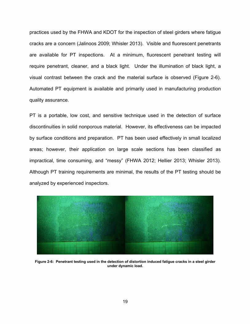
Figure 2-9: Effect of defect on wave propagation in the material using (a) Through
Transmission (TT) and (b) Pulse Echo (PE) ultrasonic testing applications. .............................. 25
Figure 3-1: Active PZT layered unimorph subjected to a displacement resulting in a moment
(Mx) applied in the longitudinal direction. .................................................................................... 31
Figure 3-2: Crack opening displacement (Δx) of an edge crack in material............................... 31
Figure 3-3: Strong and weak axis location for an H-shaped member. ....................................... 32
Figure 3-4: PACTS systems general design geometry including (a) profile view and (b) side
view of system. ........................................................................................................................... 32
Figure 3-5: Substrate geometry design progression including (a) the use of steel screws, (b)
attachment of magnets, and (c) the general substrate and leg layout. ....................................... 34
Figure 3-6: Prototype of PACTS tool. ........................................................................................ 35
ix

Figure 4-1: Reduction of stiffness matrix, C, for an isotropic material under plane-stress
conditions. ................................................................................................................................... 39
Figure 4-2: Reduction of compliance matrix, S, for an isotropic material under plane-stress
conditions. ................................................................................................................................... 39
Figure 4-3: In-Plane Forces, N, and Moments, M, on a flat surface. ......................................... 41
Figure 4-4: Geometry of N-Layered Laminate. .......................................................................... 42
Figure 4-5: Piezoelectric unimorph sensor. ............................................................................... 45
Figure 4-6: PACTS tool diagram and variables used in CLPT analysis ..................................... 46
Figure 4-7: Laminate geometry with evaluation thicknesses of piezoceramic, bond, and
substrate layers. .......................................................................................................................... 48
Figure 4-8: Two layer laminate of the driving parameters of the PACTS tool. ........................... 51
Figure 4-9: PZT and substrate dominated laminate. .................................................................. 53
Figure 4-10: PACTS tool test RC charging circuit diagram. ....................................................... 54
Figure 4-11: General relationship of sensed Voltage, Vs and time, t of RC charging circuit. ..... 55
Figure 4-12: FE model of PACTS tool layout with applied unit force ......................................... 56
Figure 4-13: Deformed shape of PACTS FE model. .................................................................. 57
Figure 4-14: Mesh size 0.0254 mm [0.001 in] in each layer of the FE model. ........................... 58
Figure 4-15: Symmetric boundary condition used in the Abaqus FE model of the PACTS
geometry. .................................................................................................................................... 58
Figure 5-1: Path of FE model mid-plane strain values used from a PZT layer with a thickness of
0.508 mm [0.020 in]. ................................................................................................................... 62
Figure 5-2: FE model results of PACTS voltage sensitivity as a function of the aluminum
substrate thickness for a 0.508 mm [0.020 in] thick PZT layer and a 0.0254 mm [0.001 in] thick
bond layer. .................................................................................................................................. 63
x

Figure 5-3: FE model results of PACTS voltage sensitivity for a 0.508 mm [0.020 in] PZT layer
thickness as a function of the aluminum thickness and bond thicknesses ranging from 0.0254
mm [0.001 in] ≤ tb ≥ 6.35 mm [0.25 in]. ....................................................................................... 64
Figure 5-4: FE model results of PACTS voltage sensitivity as a function of PZT layer
thicknesses and aluminum substrate thickness using a constant 0.0254 mm [0.001 in] bond
layer thickness. ........................................................................................................................... 66
Figure 5-5: Parametric analysis of voltage sensitivity of the PACTS tool geometry as a function
of PZT, bond material, and aluminum substrate layer thicknesses. ........................................... 67
Figure 5-6: Optimized PACTS tool geometry selected for the proof of concept testing. ............ 68
Figure 6-1: FE longitudinal mid-plane strain results for the selected PACTS tool geometry,
where tp = 0.508 mm [0.020 in], tb = 0.0254 mm [0.001 in], and ts = 1.905 mm [0.075 in],
verifying that the PZT layer is in compression under testing conditions for the selected
geometry. .................................................................................................................................... 70
Figure 6-2: Artificial Crack Test-Set illustrating the (a) labeled artificial crack specimen and
testing equipment; close up images of the (b) displacement gage, PACTS tools; and the (c)
multimeter and metronome used. ............................................................................................... 71
Figure 6-3: Voltage reading at 60 seconds using a 1000 μF capacitor and 50kΩ of resistance in
the PZT sensing circuit when a 0.381mm [0.0150 in] displacement (measured at 340 mm [13.4
in] from the artificial crack tip) is applied at a frequency of 1Hz. ................................................. 73
Figure 6-4: Acrylic compact tension specimen geometry used for the crack tip identification
testing. ........................................................................................................................................ 74
Figure 6-5: (a) Acrylic test specimen used in the in the (b) crack tip boundary identification
experiment. ................................................................................................................................. 75
Figure 6-6: Voltage readings taken at 10 mm [0.39 in] increments along the test specimen over
60 seconds at a frequency of 2.2 Hz .......................................................................................... 76
xi

Figure 6-7: Voltage reading taken over 60 seconds at frequency of 2.2 Hz with trend lines
added to the linear regions behind and ahead of the crack tip. .................................................. 77
Figure 6-8: Voltage reading along the length of the cracked specimen taken over 60 seconds at
frequency of 2.2 Hz with a line tangent to the non-linear portion that includes the location of the
crack center. ............................................................................................................................... 78
Figure 6-9: Slopes of the linear region and the constructed tangent line used to identify the
crack front boundary of the acrylic specimen. ............................................................................. 79
Figure 7-1: Edge crack with multiple cracks fronts. ................................................................... 81
Figure B-1: General H-beam geometry in milling machine. ....................................................... 89
Figure B-2: Piezoceramic sheet ................................................................................................. 90
Figure B-3: Diamond saw used to cut the piezoceramic sheets. ............................................... 90
Figure B-4: Piezoceramic sheet and 340 grit sand paper. ......................................................... 91
Figure B-5: (a) Variable speed lathe used to remove the (b) steel screw head and sharpen the
shaft tip. ...................................................................................................................................... 92
Figure B-6: Cleaned steel screw mounted to countersunk magnet. .......................................... 93
Figure B-7: PACTS tool leg assembly with sharpened steel screw and countersunk magnet... 93
Figure B-8: Two PACTS tool composite members with leads grounded to the substrate frame
and soldered to top of the piezoceramic sensor sheet. .............................................................. 94
Figure B-9: Fabricated PACTS tools. ......................................................................................... 94
Figure C-1: FE model results of PACTS voltage sensitivity for a 0.254 mm [0.010 in] PZT layer
thickness as a function of the aluminum thickness and bond thicknesses ranging from 0.0254
mm [0.001 in] ≤ tb ≥ 6.350 mm [0.250 in]. ................................................................................... 95
Figure C-2: FE model results of PACTS voltage sensitivity for a 0.508 mm [0.020 in] PZT layer
thickness as a function of the aluminum thickness and bond thicknesses ranging from 0.0254
mm [0.001 in] ≤ tb ≥ 6.35 mm [0.250 in]. ..................................................................................... 95
xii

Figure C-3: FE model results of PACTS voltage sensitivity for a 1.016 mm [0.040 in] PZT layer
thickness as a function of the aluminum thickness and bond thicknesses ranging from 0.0254
mm [0.001 in] ≤ tb ≥ 6.35 mm [0.250 in]. ..................................................................................... 96
Figure C-4: FE model results of PACTS voltage sensitivity for a 2.032 mm [0.080 in] PZT layer
thickness as a function of the aluminum thickness and bond thicknesses ranging from 0.0254
mm [0.001 in] ≤ tb ≥ 6.35 mm [0.250 in]. ..................................................................................... 96
Figure C-5: FE model results of PACTS voltage sensitivity for a 2.540 mm [0.100 in] PZT layer
thickness as a function of the aluminum thickness and bond thicknesses ranging from 0.0254
mm [0.001 in] ≤ tb ≥ 6.35 mm [0.250 in]. ..................................................................................... 97
Figure C-6: FE model results of PACTS voltage sensitivity as a function of PZT layer
thicknesses and aluminum substrate thickness using a constant 0.0254 mm [0.001 in] bond
layer thickness. ........................................................................................................................... 97
Figure C-7: FE model results of PACTS voltage sensitivity as a function of PZT layer
thicknesses and aluminum substrate thickness using a constant 1.270 mm [0.050 in] bond layer
thickness. .................................................................................................................................... 98
Figure C-8: FE model results of PACTS voltage sensitivity as a function of PZT layer
thicknesses and aluminum substrate thickness using a constant 2.540 mm [0.100 in] bond layer
thickness. .................................................................................................................................... 98
Figure C-9: FE model results of PACTS voltage sensitivity as a function of PZT layer
thicknesses and aluminum substrate thickness using a constant 5.080 mm [0.200 in] bond layer
thickness. .................................................................................................................................... 99
Figure C-10: FE model results of PACTS voltage sensitivity as a function of PZT layer
thicknesses and aluminum substrate thickness using a constant 6.350 mm [0.250 in] bond layer
thickness. .................................................................................................................................... 99
Figure D-1: (a) Artificial Crack System and close up of (b) closed crack and (c) open crack
configurations. ........................................................................................................................... 108
xiii

Figure D-2: Drawing of Artificial Crack System Main Post ....................................................... 109
Figure D-3: Drawing of Artificial Crack System Swing-arm. ..................................................... 110
Figure D-4: Drawing of Artificial Crack System Foot. ............................................................... 111
Figure D-5: Drawing of Artificial Crack System Hinge Piece 1. ............................................... 112
Figure D-6: Drawing of Artificial Crack System Hinge Piece 2. ............................................... 113
Figure E-1: Acrylic specimen geometry. .................................................................................. 117
Figure E-2: Acrylic specimen test voltage reading results at distances ahead and behind the
crack tip boundary with linear trend lines. ................................................................................. 118
Figure E-3: Acrylic specimen test voltage reading results at distances behind the crack tip and
the approximated crack tip boundary location using the using the extension on the linear portion
of the results and zero voltage. ................................................................................................. 119
Figure E-4: Acrylic specimen test voltage reading results at distances behind the crack tip and
the equation of the non-linear section used in the crack tip location analysis. ......................... 119
Figure E-5: Acrylic specimen test voltage reading results at distances behind the crack tip and
the equations of the non-linear section used in the crack tip location analysis and the line
tangent to the non-linear region through the crack tip boundary. ............................................. 120
Figure E-6: Ultimate load of 1704 N [383 lb] determined experimentally for the acrylic specimen
material used in the PACTS tool proof of concept testing. ....................................................... 122
xiv

LIST OF TABLES
Table 2-1: Summary of NDE techniques used in the inspection of in-service steel structures. . 29
Table 5-1: Laminate layer thicknesses used in the FE models generated for the optimization
study. .......................................................................................................................................... 61
Table C-1: FE model PACTS tool PZT layer mid-plane strain results and voltage sensitivity
calculations as a function of substrate and bond thicknesses using a constant 0.254 mm [0.010
in] PZT layer thickness. ............................................................................................................. 100
Table C-2: FE model PACTS tool PZT layer mid-plane strain results and voltage sensitivity
calculations as a function of substrate and bond thicknesses using a constant 0.508 mm [0.020
in] PZT layer thickness. ............................................................................................................. 101
Table C-3: FE model PACTS tool PZT layer mid-plane strain results and voltage sensitivity
calculations as a function of substrate and bond thicknesses using a constant 1.016 mm [0.040
in] PZT layer thickness. ............................................................................................................. 102
Table C-4: FE model PACTS tool PZT layer mid-plane strain results and voltage sensitivity
calculations as a function of substrate and bond thicknesses using a constant 2.032 mm [0.080
in] PZT layer thickness. ............................................................................................................. 103
Table C-5: FE model PACTS tool PZT layer mid-plane strain results and voltage sensitivity
calculations as a function of substrate and bond thicknesses using a constant 2.540 mm [0.100
in] PZT layer thickness. ............................................................................................................. 104
Table D-1: Artificial Crack System experimental results .......................................................... 114
Table E-1: Experimental results for acrylic proof of concept testing. ....................................... 118
Table E-2: Acrylic compact tension specimen ultimate load test data. .................................... 123
xv

LIST OF ABBREVIATIONS
AASHTO -- American Association of State Highway and Transportation Officials
ACS -- Artificial Crack System
AE -- Acoustic Emissions
ASCE -- American Society of Civil Engineers
ASNT -- American Society of Nondestructive Testing
Cij -- Elastic Stiffness Matrix
CLPT -- Classic Laminated Plate Theory
COD -- Crack Opening Displacement
Colt -- Crack Opening Linear Displacement
Cq-stored -- Charged stored using the PACTS tool design circuit
CT -- Computed Assisted Tomography
DFH -- Distance from PACTS Tool Centerline to Contact Surface
ε0ij -- Mid-plane Strain
εij -- Strain
κij -- Plate Curvature
Eb -- Bond Material Modulus of Elasticity
Ep -- Piezoceramic (PZT) Modulus Elasticity
Es -- Substrate (Aluminum) Modulus of Elasticity
ET -- Eddy Current Testing
f -- PACTS Tool Excitation Frequency
FHWA -- Federal Highway Administration
G -- Shear Modulus of Rigidity
g31 -- Strain Developed per Applied Charge Density where stress is Applied
in the 1-Direction and the Electrodes are Applied Perpendicular to the 3-axis
Gap -- Gap or Length of PACTS Tool Web
KDOT -- Kansas Department of Transportation
KU -- University of Kansas
LEFM -- Linear Elastic Fracture Mechanics
Mij -- Resultant Laminate Moments
MT -- Magnetic Particle Testing
NBIS -- National Bridge Inspection Standards
NDE -- Nondestructive Evaluation
xvi

NDI -- Nondestructive Investigation
NDT -- Nondestructive Testing
NHI -- National Highway Institute
Nij -- Resultant Laminate Forces
PACTS -- Piezoelectric Active Crack Tip Sensor
PAUT -- Phased Array Ultrasonic Testing
PAWS -- Piezoelectric Wafer Active Sensors
PE -- Pulse Echo
POD -- Probability of Detection
PT -- Penetrant Testing
PZT -- Lead-Zirconate-Titanate
Qij -- Reduced Elastic Stiffness Matrix
R -- Resistance
RT -- Radiography Testing
SHM -- Structural Health Monitoring
Sij -- Compliance Matrix
tb -- Bond Layer Thickness
tp -- PZT Layer Thickness
ts -- Substrate Layer Thickness
TT -- Through Transmission
U.S. -- United States
UT -- Ultrasonic Testing
ν -- Poisson's Ratio
VI -- Visual Inspection
Vpiezo -- Voltage in the PZT Layer
Vsensed -- Voltage Sensed by the PACTS System
VT -- Visual Testing
W -- Width of PACTS tool flanges
Δx -- Crack Opening Displacement
xvii

PAGE LEFT INTENTIONALLY BANK
xviii

CHAPTER 1: INTRODUCTION 1.1 Research Motivation
In 2013, the condition of the nation’s bridge infrastructure was reported as “mediocre”
and received a C+ in ASCE’s Infrastructure Report Card. This rating is primarily due to
the structural condition of the 607,380 bridges within the Federal Highway system and
the growing cost associated with their condition (ASCE 2013). The average age of the
United States’ (U.S.) bridge infrastructure is forty-two years and nearly 11% of these
structures are classified as structurally deficient (FHWA 2011). With the majority of
these bridges exceeding their initial 50 year design life and replacement of each
structure financially unfeasible, it is important to monitor and assess their structural
capacity on a routine basis in order to identify maintenance and repair needs.
Therefore, reliable and efficient inspection methods and techniques must be explored
and developed to assist in the overall analysis of a bridges ability to maintain its
structural stability under service loads.
Since approximately 30% (181,000) of the nation’s bridge inventory are steel structures,
it was determined that the development of a viable inspection tool could assist
inspectors in the identification of active cracks within steel members. Early crack
detection can assist bridge maintenance personnel in developing cost-effective
maintenance and repair plans in lieu of high cost bridge replacements. Additionally,
early crack detection allows bridge engineers to evaluate the remaining service life of
the structure and prioritize repair and replacement needs based on available funding.
1

1.2 Research Objective
The objective of this dissertation was to evaluate the use of a Lead-Zirconate-Titanate
(PZT) piezoceramic material as an active sensor in the detection and characterization of
cracks in steel structures. PZT sensors were selected due to their ability to convert the
small mechanical displacements into electrical signals including voltage or charge. The
sensitivity of the PZT and design of the substrate geometry accurately identified active
cracks in a material and the location of the crack tip. The design presented in this
dissertation will provide bridge engineers an opportunity to conduct bridge inspections
and detect crack growth without requiring large scale equipment. Additionally, the
accurate identification of the crack tip location could assist bridge engineers and
managers in the development and implementation of accepted repair techniques
including the drilling of crack arrest holes.
The new Piezoelectric Active Crack Tip Sensor (PACTS) inspection tool was
investigated through a proof-of-concept testing program that included experimental
testing, numerical modeling, and closed form solutions. This research resulted in the
development of a compact and portable crack detection system that can be used to
monitor and investigate crack activity in metallic structural elements using piezoelectric
materials.
1.3 Organization of the Dissertation
This dissertation is divided into seven chapters in addition to five appendices.
Chapter 1 defines the motivation and research objective in addition to the
organizational layout of the dissertation.
2

Chapter 2 identifies the background information related to the benefits of
inspections and advanced nondestructive techniques used in the identification of
cracks and defect within bridge structures. This chapter also presents a brief
literature review of piezoelectric materials and their applications in bridge
inspection and structural health monitoring techniques.
Chapter 3 summarizes the material selection process used to create the general
design of the PACTS tool.
Chapter 4 outlines the modeling methods and techniques used for the PACTS
tool analysis including finite element analyses and closed form solutions using
classic laminated plate theory.
Chapter 5 is a presentation of the optimization process used to identify a tool
geometry that would be used for experimental testing.
Chapter 6 is the Proof of Concept section that presents the finite element
analysis and test results that illustrate the sensing capabilities of the PACTS tool.
Chapter 7 provides a summary of the research findings, conclusion, and a
recommendation of future work.
The five appendices provide additional details related to the tool material properties,
finite element analysis input parameters, test and manufacturing procedures, design
plans, optimization results, and the raw data from experimental testing.
3

CHAPTER 2: LITERATURE REVIEW & BACKGROUND The development of a new inspection tool and sensor required a fundamental
understanding of fatigue and fracture concepts, types of bridge inspections, and bridge
inspection methods currently in use. This chapter will provide a brief overview of fatigue
and fracture including its application in the analysis of in-service structures. Afterwards,
the identification of the bridge inspection types and inspection methods used will be
presented, including current applications of PZT in the in the inspection of existing
structure.
2.1 Fracture Mechanics Overview
Steel structures are subjected to routine inspection in order to identify discontinuities
within the material of structural members. Discontinuities can include variations in
microstructure, cracks, laps, and inclusions. This section provides an introduction into
the area of fatigue and fracture mechanics and the effects of crack lengths and location
on the integrity of structural components. Cracks are considered narrow planar
discontinuities in a materials that were previously or should be continuous (Hellier
2013). Cracks are typically the result of fabrication techniques, event-induced damage,
or the effects of continuous operation under service conditions. They can appear as
surface, subsurface, and internal cracks.
When dealing with fracture mechanics or fatigue, it is important to understand the
difference in ductile and brittle material failure. Ductile materials undergo and are
primarily dominated by a yielding period prior to fracture and/or breakage, while brittle
materials have little if any yielding or deformation prior to failure. Brittle fracture is a
type of failure in structural materials that usually occurs without prior plastic deformation
4

and at extremely high speeds, up to 2133 m/s [7000 ft/s] in steels (Barsom and Rolfe
1999). They occur with little or no elongation or reduction in area and with very little
energy absorption. Primarily design considerations prefer ductile materials that may
exhibit some signs of distress while undergoing yielding prior to ultimate failure. Since
the failure of most structures including bridges, buildings, airplanes pose a significant
danger to public health, safety, and welfare, it is important to inspect and monitor cracks
or other discontinuities within these structures.
2.1.1 Fracture Mechanics
Fracture mechanics, in general, is the study of cracks and crack propagation. It plays a
significant role in improving the performance and life of mechanical structures and their
components. Fracture mechanics applies strength of material properties including
stress and strain to assist in the design and maintenance of various structures. When
discussing fracture mechanics, it is important to identify the primary modes or
movements of crack surfaces. There are three types of crack surface displacements
(Figure 2-1). In Mode I or opening mode, the two fractured surfaces are perpendicular
to each other and are being “pulled” in opposite directions and appear to open the
crack. In Mode II or shear mode, the two fracture surfaces slide over each other
perpendicular to the crack. This mode appears to attempt to “shear” off the two
surfaces. Mode III or tearing mode, is where the two surfaces slide over each other in a
direction parallel to the crack front (Barsom and Rolfe 1999). Mode III produces a
“scissoring motion” at the crack front (Sanford 2003). Primarily Mode I, opening mode,
is considered the most important mechanism controlling failure, since growing cracks
tend to position themselves in a direction to minimize or eliminate the effects of Mode II
5

and III (Sanford 2003). This research and proof of concept study focused on Mode I
crack surface displacements.
Figure 2-1: Three basic modes of crack surface displacements (Barsom and Rolfe 1999).
A number of large structures including aircraft, pressure vessels, buildings and bridges
have initial imperfections that resemble cracks. These imperfections can be sharp
notches or discontinuities in the material. Fracture mechanics can be used in the
design, inspection, and forensic analysis of these types of structures. Fracture
mechanics allows engineers to determine allowable stress levels on a structure with a
known flaw size; to determine inspection times by allowing engineers to calculate the
critical crack size at failure for a member; and it can be used to determine the fatigue
crack growth rate to establish an acceptable design life of a new structure or the fatigue
6

life of a pre and post in-service structure. The use of fracture mechanics after a
structural failure in forensic analysis can help identify crack initiation points which could
potentially establish responsibility and accountability of any catastrophic failures.
The implementation of fracture mechanics principles in design and analysis procedures
can be instrumental in providing safe and cost effective structural elements and
facilities. The concepts of fracture mechanics can be simplified into basic engineering
principles including stress, strain, and material properties. The driving force for fracture
mechanics is the stress intensity factor, KI, which is analogous to the calculated nominal
stress. The relationship between stress intensity factor, KI, the applied stress, σ, and
the crack size, a, for three crack geometries is shown in Figure 2-2. The Edge Crack
geometry was used to analyze the effectiveness of the PACTS tool.
Figure 2-2: Stress Intensity factor, KI, values for different crack geometries (Barsom and Rolfe 1999).
The resistance force or the fracture toughness, KC, is a material property similar to the
yield strength of materials used in design. Fracture toughness is the amount of energy
a material can absorb before brittle failure. It describes the material’s resistance to
fracture and can be determined by integrating the area under the stress-strain curve or
experimentally using ASTM International test standards (2012). KI and KC can be used
in the design and assessment of structures by assisting engineering in determining
7

allowable stress ranges, critical flaw sizes, and selecting materials that would optimize
the design of metal structures (Figure 2-3).
Figure 2-3: Relationship between stress, initial flaw size, and material toughness (Barsom and Rolfe 1999).
2.1.2 Fatigue
In the previous section the fracture behavior was outlined for flaws under monotonically
increasing loads. However, most structures including bridges, ships, and aircraft are
subjected to repeated loads that may fluctuate in magnitude (Barsom and Rolfe 1999).
Fatigue damage in structures occurs due to repeated loading that is usually below the
allowable yield strength of the material used. This occurs due to stress risers or regions
where the localized stress exceeds the yield stress of the material. Stress risers can
include welds, imperfections, and geometrical changes in non-welded components.
After numerous cycles of load fluctuation, the localized material damage can initiate a
fatigue crack and then propagate the crack throughout the member. Fuchs and
Stephens stated in their 1980 text that “the ultimate cause of all fatigue failures is that a
8

crack has grown to a point at which the remaining material can no longer tolerate the
stresses or strains, and sudden fracture occurs” (1980). The total fatigue life of a
structure, Nt, includes the number of loading cycles required to initiate a crack, Ni, and
the number of cycles to propagate the crack, Np (Equation 2:1).
𝑁𝑡 = 𝑁𝑖 + 𝑁𝑝 Equation 2:1
When analyzing fatigue crack growth, it is important to note that the crack propagation
rate is dependent on the change in crack size (Δa) and the applied stress range (Δσ).
Therefore accurate and quality inspection reports identifying cracks and crack growth
can be used in evaluation of fatigue life and propagation, thus assisting maintenance
departments in determining retrofit, repair, or replacement requirements for their
structures inventory.
Based on the information used to determine the fatigue life and the relationship between
the applied stress, flaw size, and fracture toughness (Figure 2-3), it can be concluded
that to increase the fatigue life of a structure, a designer should consider lowering the
stress range (Δσ), minimizing the flaw size (Δa), or increasing the fracture toughness of
the materials used. Literature indicates that reducing the flaw size or the stress range
for structure provides a larger effect on the fatigue life then increasing the toughness of
the material (Barsom and Rolfe 1999; Fuchs and Stephens 1980; Sanford 2003).
However, in order to decrease the applied stress range of an in-service bridge structure,
it typically requires restricting traffic loads by reducing the posted load limit of the bridge.
This method is effective at extending the fatigue life, but it is not a viable option in rural
or remote locations where alternative routes are unavailable. Therefore, early crack
identification is a significant factor in establishing and extending the fatigue life of a
9

structure. Early crack identification can be used by bridge engineers in the design,
selection, and application of feasible retrofit materials and techniques, which could
result in the use of higher KC materials that can increase fatigue life. Therefore, proper
inspections that accurately identify and characterize cracks can be used to analyze and
monitor the structural performance and fatigue life and minimize the potential effects
and disruptions to traffic patterns and commute times.
2.1.3 Fitness for Service
The same principles and practices used in design to prevent fracture failure can be
used to evaluate in-service bridges and potentially extend service life. The average age
of the nation’s bridges is forty two years and they are steadily approaching their initial
design life (FHWA 2011). A Fitness for Service assessment considers the age of a
structure in addition to its actual in-service loading conditions, crack or flaw sizes, and
the material toughness (Wells 1981). Fitness for Service was initially described by Alan
Wells in the early 1960s and more recently referred to as “common sense engineering”
by Stanley Rolfe (1993). Fitness for Service analysis can be conducted pre or post in-
service conditions. Although there are no specific guidelines for the fitness for service
procedure in bridge inspections, the American Society for Mechanical Engineers
(ASME) has outlined a procedure using fracture mechanics principles to determine the
maximum acceptable flaw size that can be tolerated before exceeding allowable values
in nuclear power plant components (2010). The fundamental first step of their
procedure includes performing a quality inspection that identifies and characterizes
actual flaw sizes and locations. However, in order to successfully identify cracks it is
important to identify the types of inspections conducted on in-service bridge structures.
10

2.2 Types of Bridge Inspections
Inspection of transportation structures assists owners in ensuring the safe passages of
people and goods across the federal highway system. If properly conducted and
documented, regular and sporadic inspections of bridges can help ensure the structural
integrity of its members and provide pertinent information necessary to properly
maintain each structure. Throughout the life of a bridge structure, the type of inspection
conducted may vary depending on the structural integrity and age of the structure and
its members. In accordance to the American Association of State Highway and
Transportation Officials (AASHTO) Manual for Bridge Evaluation, there are seven
bridge inspection types (2008).
• Initial Inspection
An Initial Inspection is the first inspection conducted on a new or widened bridge
structure. This inspection identifies the required information regarding the bridge
geometry, layout, and length that is recorded in the structure’s inventory record.
Additionally, it defines the baseline condition of the bridges structural members
and identifies any existing problem.
• Routine Inspection
A Routine Inspection is a periodic inspection conducted on a regularly scheduled
basis. This inspection type is used to determine the physical and functional
condition of a bridge. Current conditions are compared to previous Routine and
Initial inspection condition ratings to ensure the bridge meets its serviceability
requirements. Routine inspections are typically conducted from the ground or
deck level and may not include a hands-on inspection of individual structural
11

members. It provides a cursory inspection of the overall structure. Routine
inspections are required and satisfy the National Bridge Inspection Standards
(NBIS) requirements for periodic comprehensive inspections of in-service
structures.
• In-Depth Inspection
In-Depth Inspections include a hands-on inspection of one or more bridge
members. They are also conducted in order to identify potential deficiencies that
were not investigated or detectable during Routine Inspections. In-Depth
inspections may require the use of additional nondestructive testing (NDT)
techniques outside of visual inspection.
• Special Inspection
Special Inspections are conducted in order to evaluate and monitor known
defects or conditions, including areas susceptible to distortion induced fatigue
cracking and foundation settlement or scour. Since the inspected area is
localized, Special Inspections do not meet the NBIS requirements for
comprehensive periodic inspections. The inspections are typically conducted by
inspectors familiar with potential consequences of the deficiency and skill in the
inspection method required to adequately evaluate the structural performance.
12

• Fracture-Critical Inspection
Fracture-Critical Inspections are performed on steel bridges with fracture critical
members whose failure would probably result in the inability of the bridge
structure to perform its load carrying function and/or the collapse of a portion or
the entire bridge. This inspection type includes the identification of fracture
critical members and the development of a plan to inspect these members.
• Underwater Inspection
Underwater Inspections are conducted on channel crossings to locate the bottom
of the channel and determine the structural integrity of underwater substructure
components, by identifying and evaluating scour and undermining conditions.
This inspection type can be conducted from above the water surface level for
shallow crossings but may require diving or other techniques in deeper waters.
• Damage Inspection
Damage Inspections are unscheduled inspections conducted in order to assess
the structural damage resulting from environmental factors including hurricanes
and earthquakes in addition to human actions such as over height truck strikes of
low clearance bridge structures as illustrated in Figure 2-4. The primary goal of
Damage Inspection is to determine if there is a need for further action including
structural repair and/or emergency load restrictions, or replacement.
13

Figure 2-4: Tractor trailer collision resulting in a non-scheduled Damage Inspection to evaluate the
structural integrity of the steel deck plate girder bridge. (Photo Credit: A. Elmore, NY)
Each inspection method described in this section requires trained and qualified
personnel and all inspections should be documented and filed for future review. During
inspections, where cracks are identified, it is important to properly characterize each
crack by documenting the crack location, length, and size.
2.3 Civil Infrastructure Inspection Methods
Routine inspections are typically conduced every two years on bridge structures within
the United States (U.S.). Although the U.S. has approximately 200,000 steel bridges,
visual nondestructive evaluations (NDE) are still the primary inspection method used,
with occasional validation performed using dye penetrant and magnetic particle tests
(FHWA 2011; NDEC 2010). The probability of detection (POD) using visual techniques
varies greatly and may be highly impacted by human behavior and environmental
factors and conditions (FHWA 2001; Hellier 2013). Advanced NDE methods used in the
14

inspection of steel bridge structures include ultrasonic, eddy current, radiography, and
acoustic emissions These advanced methods have been investigated by the Federal
Highway Administration’s (FHWA) NDE Center, and have been successful in helping to
identify surface or near-surface cracks on steel bridge systems (NDEC 2010).
However, the usage of these advanced techniques is limited to “special,” non-routine
bridge inspections. During routine inspections, bridge inspectors typically visually
identify cosmetic imperfections that appear to be “active” cracks then document and
recommend the use of advanced techniques to verify and characterize cracks and
volumetric changes within the structure.
Nondestructive Testing Evaluation or Testing (NDE/NDT) techniques used for structural
evaluation allow inspectors and maintenance personnel to evaluate the structural
condition and/or integrity of the bridge without invasive destructive testing requirements.
NDT methods can identify maintenance and repair needs during inspections and helps
to identify structural health monitoring (SHM) needs which involves providing continuous
monitoring of in-service structures. The NDE methods outlined in this section include
visual, dye penetrant, magnetic particle, eddy current, and radiography test methods.
Additionally, piezoelectric materials are introduced and their application in ultrasonic
and acoustic emissions testing.
When considering the effectiveness of inspection techniques used, the probability of
detection (POD) is the method generally used. POD is the probability of detecting a
given crack or discontinuity under specific conditions and techniques. Although, the
POD values vary depending on the method or technique used, it is important to note
that generally the POD of an inspection method increases with increasing flaw or crack
15
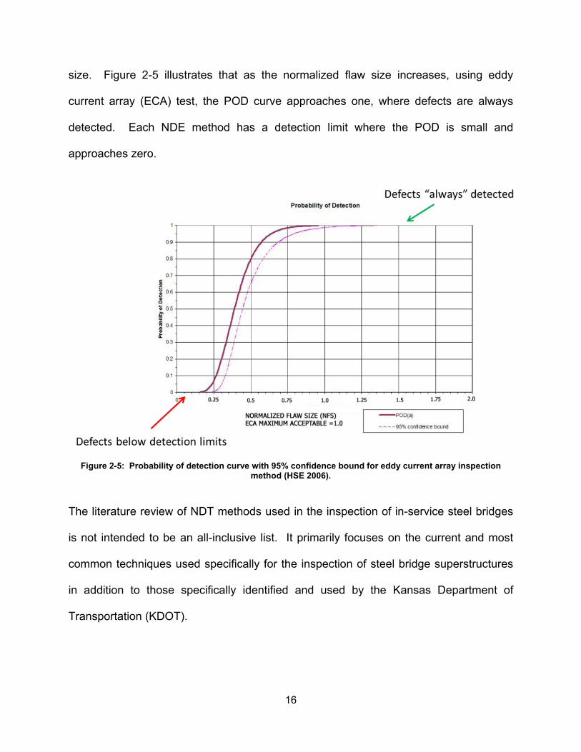
size. Figure 2-5 illustrates that as the normalized flaw size increases, using eddy
current array (ECA) test, the POD curve approaches one, where defects are always
detected. Each NDE method has a detection limit where the POD is small and
approaches zero.
Figure 2-5: Probability of detection curve with 95% confidence bound for eddy current array inspection
method (HSE 2006).
The literature review of NDT methods used in the inspection of in-service steel bridges
is not intended to be an all-inclusive list. It primarily focuses on the current and most
common techniques used specifically for the inspection of steel bridge superstructures
in addition to those specifically identified and used by the Kansas Department of
Transportation (KDOT).
16

2.3.1 Visual Inspection
Visual Inspection (VI) methods evaluate the presence of surface discontinuities with the
use of normal eyesight alone or the addition of optical instruments including magnifying
glasses, artificial light, and or mirrors. VI is the most commonly used method of
structural evaluation and is considered a cost effective means of evaluating surface
discontinuities of various structural components or an entire bridge system (FHWA
2001; Hellier 2013; Purvis 1988; Whisler 2013). Typical discontinuities identified using
VI methods include corrosion, the misalignment of parts, physical and cosmetic
damage, and surface cracks. VI is the initial safe guard in minimizing crack growth and
brittle failure. The results of VI are used in the monitoring of bridge condition and
scheduling of bridge maintenance.
In 2001, the FHWA published a report that investigated the reliability of visual
inspection. During their investigation, 49 inspectors from 25 state transportation
agencies were evaluated. It was determined that the inspection reports had “significant
variability” between inspectors. The variation in assigned bridge condition ratings
correlated with individual inspectors’ Fear of Traffic, Visual Acuity and Color Vision,
Light Intensity, Inspector Rushed Level, and the perceptions of Maintenance
Complexity, and Accessibility (FHWA 2001). It was also noted that the independent use
of VI for In-Depth or Special Inspections may not identify any deficiencies outside of
those located during Routine Inspections.
Although VI results and observations vary, its significance in the area of bridge
inspections was adequately described by Purvis in the following statement:
17
“In most situations the only method available to detect flaws in a bridge member
is visual inspection. It is important to identify the flaws early in the typical crack-
development scenario. If the defect is identified as soon as it can be seen by the
inspector, the service life of the member often has been reduced by more than
80 percent (Purvis 1988).”
VI is the first method of defect detection used within the inspection industry. VI can be a
low cost effective means of inspection. Training requirements are primarily experience
based and require little advanced training. However, VI results can vary depending on
the inspector’s ability and overall thoroughness. Using the method of VI, may require
that the area to be inspected be cleaned including the removal of debris, paint, or rust.
Additional lighting or other optical stimulation may be required to adequately inspect
critical areas. Inspectors using this method should be familiar with the area susceptible
to cracking; be able to identify the crack; and be willing to get close enough to visually
see the crack. Cracks identified using VI are typically validated using advanced
inspection techniques.
2.3.2 Advanced Techniques
2.3.2.1 Liquid or Dye Penetrant
The application of a viscous liquid or dye to the surface being inspected enhances the
appearance of surface discontinuities in solid nonporous materials. Penetrant testing
(PT) utilizes capillary action of the surface to pull penetrant into the surface
discontinuities. The application of PT is used in detection of sharp fatigue cracks and is
usually selected based on the results of VI. Properly used PT can also help determine
the extent of a crack already identified by VI. Dye penetrant is one of the two standard
18
practices used by the FHWA and KDOT for the inspection of steel girders where fatigue
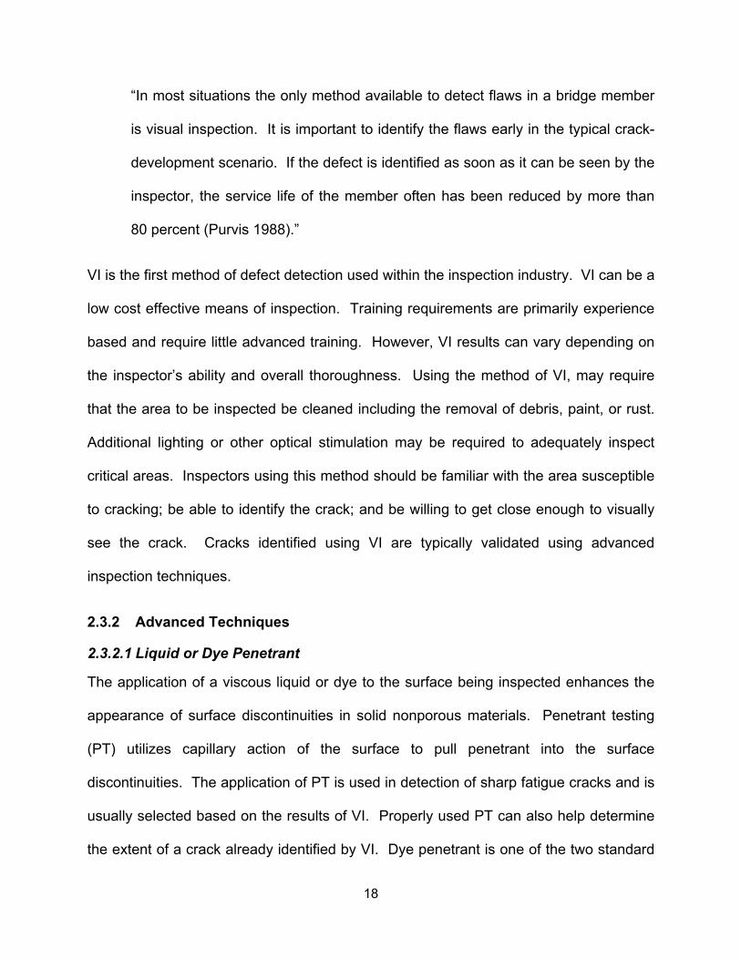
cracks are a concern (Jalinoos 2009; Whisler 2013). Visible and fluorescent penetrants
are available for PT inspections. At a minimum, fluorescent penetrant testing will
require penetrant, cleaner, and a black light. Under the illumination of black light, a
visual contrast between the crack and the material surface is observed (Figure 2-6).
Automated PT equipment is available and primarily used in manufacturing production
quality assurance.
PT is a portable, low cost, and sensitive technique used in the detection of surface
discontinuities in solid nonporous material. However, its effectiveness can be impacted
by surface conditions and preparation. PT has been used effectively in small localized
areas; however, their application on large scale sections has been classified as
impractical, time consuming, and “messy” (FHWA 2012; Hellier 2013; Whisler 2013).
Although PT training requirements are minimal, the results of the PT testing should be
analyzed by experienced inspectors.
Figure 2-6: Penetrant testing used in the detection of distortion induced fatigue cracks in a steel girder under dynamic load.
19

2.3.2.2 Magnetic Particle
Similarly to PT, magnetic particle testing (MT) is used in combination with VI in order to
locate surface and near-surface discontinuities in materials that are capable of being
magnetized. In MT, a magnetic field is applied to the material surface, then iron or
magnetic iron oxide particles are sprayed over the magnetized surface. The magnetic
particles attach to the edges of the defect in order to reveal its location. In dark non-
illuminated areas, the location of the attached fluorescent particles can be determined
using ultraviolet light, therefore producing a visual contrast between the particles and
the material surface (Hellier 2013; Jalinoos 2009). Additionally, magnetic particle is one
of the two standard practices used by the FHWA for the inspection of steel girders
where fatigue cracks are a concern (Jalinoos 2009).
MT advantages include rapid test results within minutes of particle application and
easily interpretable results for surface and near surface discontinuities. MT is a
versatile technique where variations in particle sizes can identify different crack sizes
and provide sharper imaging. Similarly to PT, MT has been used effectively in small
localized areas; however, their application on large scale sections has been classified
as impractical and time consuming (FHWA 2012; Hellier 2013; Whisler 2013).
2.3.2.3 Eddy Current
Eddy Current testing (ET) uses an electrical circuit or coil to create a magnetic field.
The coil is then placed over a conductive material where opposing alternating currents,
or eddy currents, are generated. When the generated current flow is obstructed by a
defect, it results in a change in the electromagnetic field. Eddy current electromagnetic
field changes can be identified on an oscilloscope.
20

ET is one of the primary NDE tools used on steel structures to identify surface and near
surface cracks (Jalinoos 2009; Whisler 2013), especially at weld connections. When
properly positioned, ET can accurately locate defects and identify the crack tip. In order
to correctly locate and identify defects using ET, the defect must cross the eddy current
flow as shown in Figure 2-7. However, the probes sensitivity to magnetic particles
including weld materials can influence ET results. Other limitations include the training
requirements to operate and interpret ET results as well as high equipment cost. ET
testing is a time consuming method of inspection that requires large equipment and
focuses on localized areas (Hellier 2013; Whisler 2013).
Figure 2-7: Pancake - type coil applied to a flat surface with the defect crossing the eddy currents.
2.3.2.4 Radiography
Radiography is a through transmission inspection tool that provides a volumetric
inspection of a solid surface by penetrating x-rays or gamma rays through the material.
In traditional scans, the through transmission results appear on the radiographic film
located on the other side of the test specimen Figure 2-8. However, if only one side of
21

the material is accessible, a backscatter technique can be employed. Radiography
testing (RT) use is limited due primarily to radiation exposure safety concerns.
Exposure time, dosage, and the distance from the source should be monitored to limit
potential adverse radiation effects.
Figure 2-8: Image of Radiography test set-up.
Computed Assisted Tomography (CT) is a radiographic method that uses penetrating
radiation from radioisotope or x-ray tube sources. These results produce cross-
sectional images that include variations in material density. Similarly to radiography, CT
sensitivity requires proper alignment of the radiation beam and the flaw or discontinuity.
Therefore, there is difficulty in detecting cracks that were not located and characterized
during previous inspections or using alternate techniques.
Various industry applications have employed radiographic inspection techniques,
including manufacturing, food processing, shipping and RT is well known for its airport
22

security applications. Radiography is not a primary inspection technique used by
KDOT. However, it provides quality images and documentation on volumetric defects
within the material.
The quality of the images produced by RT can be affected by the characteristics of the
imaging plate. Improvements on the effectiveness of the imaging plate can be achieved
by increasing the plate thickness. However, an increase in plate thickness would result
in a decrease in image resolution (Silva et al. 2014).
2.4 Piezoelectric Materials and Inspection Applications
2.4.1 Fundamental Properties of Piezoelectric Elements
Piezoelectric materials are those materials that are capable of converting mechanical
movement into electrical outputs and vice-versa. This phenomenon is commonly
referred to as the piezo-effect and it is limited to specific crystalline structures.
Demonstrated and explored by Pierre and Jacques Cure in 1880, piezoelectric
materials have been used in NDT application within aircraft, civil, and pipe structures.
Piezoelectric materials are typically lightweight, low cost, brittle materials with high
sensitivity. The fundamental property of piezoelectric materials allows it to be used in
various applications as an actuator or a sensor. As an actuator, the piezoelectric
material is subjected to an applied voltage which results in a mechanical displacement
of the material. Conversely as an actuator, a mechanical strain can be applied to the
piezoelectric material which results in a voltage or electrical change in the material.
Natural and synthetic piezoelectric materials are available in various sizes and
sensitivities. Natural piezoelectric materials include quartz and tourmaline and synthetic
piezoelectric ceramic materials include those composed of Barium-Titanate and the
23

most commonly used Lead-Zirconate-Titanate (PZT). PZT and other manufactured
polycrystalline ceramics are available in various geometries and can be produced with
specific chemical and piezoelectric characteristics (Morgan Advanced Materials 2009;
Piezo Systems Inc. 2011). Piezoelectric materials and devices can be found in
cigarette lighters, grill igniters, smoke detectors, fish finders, and audio transducers.
In the field of NDE, piezoelectric transducers are commonly used to inspect bridge
superstructure components, including pins, rollers, and gusset plates. They are also
used in the SHM of steel structures to identify and monitor crack growth. Piezoceramic
transducers convert electrical energy into acoustical energy. This phenomenon is
commonly used in the field of bridge inspections in the form or Ultrasonic Testing and
Acoustic Emissions.
2.4.1.1 Ultrasonic Testing
Ultrasonic Testing (UT) transmits high frequency sound waves through a material to
identify cracks, voids, and other discontinuities in the material. When a discontinuity is
in the path of the sound wave, part of the energy will be reflected back from the flaw
surface. Then the reflected wave is transformed into an electrical signal by the
transducer and displayed on an oscilloscope. UT is a versatile tool that can be used
when access to both sides of the specimen is available using through transmission (TT)
or when access to one side is limited using pulse echo (PE).
UT is primarily used for pin, bolt, and weld inspections. UT imaging can provide length
and thickness measurements of discontinuities. In addition to surface discontinuities,
UT is capable of detecting subsurface discontinuities in various structural elements
including pressure vessels, piping, aircraft, machinery, and bridges.
24
Figure 2-9: Effect of defect on wave propagation in the material using (a) Through Transmission (TT) and (b)
Pulse Echo (PE) ultrasonic testing applications.
Currently Phased Array Ultrasonic Testing (PAUT) is the UT method of choice used for
the detection of cracks by the FHWA’s NDE facility (FHWA 2012). PAUT systems
contain multiple arrays of ultrasonic transducers. The use of multiple transducers
provides a cross section view of the material to help accurately identify and characterize
defects.
UT is highly accurate and sensitive to surface and subsurface discontinuities. UT
requires minimal surface preparation and provides immediate results. However, UT
testing requires high cost equipment and extensive training in order to accurately
identify discontinuities and analyze test results (Hellier 2013; Whisler 2013).
2.4.1.2 Acoustic Emissions
In the field of SHM, Acoustic Emissions (AE) is one of the commonly used tools for steel
highway structures and has shown great promise due to its ability to sense or detect
sudden energy releases within a material (FHWA 2012; Hellier 2013). The energy
released is in the form of acoustic stress waves. The use of AE as a SHM system
25

allows for continuous monitoring of the structure without requiring direct access to the
crack. However, under continuous monitoring applications AE only estimates crack
growth and should be used with other NDE methods to successfully characterize crack
sizes.
2.4.1.3 Other Applications
In addition to basic UT and AE applications, piezoelectric materials are commonly used
as actuators and sensors; however, the sensing ability has proven to be highly effective
in strain sensing applications. Similarly to traditional foil strain gages, PZT sensors are
capable of accurately measuring strain levels; however, PZT sensors tend to show
higher sensitivity to low strain levels than foil strain gages (Chopra and Sirohi 2013).
Research results have shown that PZT sensors are capable of generating their own
usable signal in response to applied force, strain, pressure, and acceleration without the
application of external energy. Piezoelectric sensors, have higher strain sensitivity than
traditional passive sensors including foil strain gages, up to one million times greater,
and they can be used in conditions with high noise levels (Gautschi 2002; Sirohi and
Chopra 2000; Yu et al. 2011).
Piezoceramics are being used as actuators and active sensors in various inspection
applications within civil and aerostructure field including the following projects:
Ihn et al. (2004) investigated the use of piezoelectric actuators to generate
diagnostic signals within an aircraft to detect fatigue crack growth in a repaired
structure. The sensor was installed in a composite repair patch bonded to
riveted fuselage joints and a cracked metallic plate. The results of this research
26

indicate that the use of piezoelectric actuator/sensor within the repair patch
successfully detected fatigue crack growth and the debonding of the patch.
Lynch (2004) researched the use of active wireless sensors to emit acoustic
waves under extreme loading conditions, including seismic loads, to monitor and
detect damage in steel moment frames. This monitoring concept was tested
using PZT actuation and sensing pads mounted to the surface of an aluminum
plate. Of the two PZT pads attached to the aluminum, one was used as an
actuator to excite the plate, and the other pad was used as a sensor to detect
scatter in the acoustic waves traveling through the plate.
Zhang (2006) used polymer based piezoelectric paint as a strain sensor to detect
surface cracks in structures. Results indicate the successful detection in real-
time monitoring of surface fatigue cracks.
Yu et al. (2011) adapted piezoelectric wafer active sensors (PAWS) to detect AE
events during SHM of steel bridges under fatigue loading scenarios. Tests were
conducted on steel and aluminum compact tension specimens and results
demonstrated that the PAWS measurement and crack mouth opening
displacement (CMOD) correlated to the acoustic activities measured using
commercially available AE software.
2.4.2 Advantages and Disadvantages
As previously outlined, piezoelectric materials are highly sensitive, comparatively low
cost materials that can be used in an array of NDT applications. However, they must be
properly monitored and maintained to ensure accuracy. Piezoelectric limitations include
temperature, voltage, and mechanical stress effects on the polarization of the ceramic
27

material (Gautschi 2002). Piezoelectric sensing or actuating performance decreases,
as the operating temperature increases due to the depolarization of the piezoelectric
material. Each piezoceramic material has a maximum temperature exposure limit, or
Curie point, where all piezoelectric properties are lost. Continuous operation of a
piezoceramic material decreases the maximum temperature limit. An introduction into a
strong electric field with opposing polarity will also depolarize piezoceramic materials.
Additionally, large mechanical stresses can effectively decrease the polarization of
piezoceramic. At elevated temperature levels, the maximum safe stress level and
overall performance is decreased and the aging process is accelerated. For more
complex detection methods, nontrivial processing and interpretation algorithms are
necessary which drives up cost, equipment size, bulk and challenges associated with
field applications (CTS 2013; Hellier 2013; Morgan Advanced Materials 2009; Piezo
Systems Inc. 2011).
2.5 Summary
Purvis’ description of the significance on VI and the essence of fracture mechanics
presented by Barsom and Rolfe (1999), identifies the importance of inspection,
inspection frequency, inspection method selection, and accurate crack detection in
establishing the service life of a structure. Quality inspections and proper crack
characterization allow maintenance officials and bridge owners to develop or select an
optimal maintenance and monitoring schedule to preserve or extend the life of bridge
structure. Each method outlined in this chapter is summarized in Table 2-1.
28

Table 2-1: Summary of NDE techniques used in the inspection of in-service steel structures (Hellier 2013).
Method Principles Application Advantages Limitations Visual Testing (VI)
Uses reflected or transmitted light from test object that is imaged with human eye or other light-sensing device
Many applications in many industries ranging from raw material to finished products and in-service inspection
Can be inexpensive and simple with minimal training required. Broad scope of uses and benefits
Only surface conditions can be evaluated. Effective source of illumination required. Access necessary
Penetrant (PT)
A liquid containing visible or fluorescent dye is applied to surface and enters discontinuities by capillary action
Virtually any solid nonabsorbent material having uncoated surfaces that are not contaminated
Relatively easy and materials are inexpensive. Extremely sensitive, very versatile. Minimal training.
Discontinuities open to the surface only. Surface condition must be relatively smooth and free of contaminants.
Magnetic Particle (MT)
Test part is magnetized an fine ferromagnetic particles applied to surface, aligning at discontinuity
All ferromagnetic materials, for surface and slightly subsurface discontinuities; large and small parts
Relatively easy to use. Equipment/material usually inexpensive. Highly sensitive and fast compared to PT
Only surface and few subsurface discontinuities can be detected. Ferromagnetic materials only.
Radiography (RT)
Radiographic film is exposed when radiation passes through the test object. Discontinuities affect exposure
Most materials, shapes, and structures. Examples include welds, castings, composites, etc., as manufactured or in-service
Provides a permanent record and high sensitivity. Most widely used and accepted volumetric examination.
Limited thickness based on material density. Orientation of planar discontinuities is critical. Radiation hazard.
Ultrasonic (UT)
High-frequency sound pulses from a transducer propagate through the test material, reflecting at interfaces
Most materials can be examined if sound transmission and surface finish are good and shape is not complex.
Provides precise, high-sensitivity results quickly. Thickness information, depth, and type of flaw can be obtained from one side of the component.
No permanent record (usually). Material attenuation, surface finish, and contour Requires couplant.
Eddy Current (EC)
Localized electrical fields are induced into a conductive test specimen by electromagnetic induction
Virtually all conductive materials can be examined for flaws, metallurgical conditions, thinning, and conductivity
Quick, versatile, sensitive; can be non-contacting; easily adaptable to automation and in situ examinations
Variables must be understood and controlled. Shallow depth of penetration, lift-off effects and surface condition.
Acoustic Emission (AE)
As discontinuities propagate, energy is released and travels as stress waves through material. These are detected by means of sensors
Welds, pressure vessels, rotating equipment, some composites and other structures subject to stress or loading.
Large areas can be monitored to detect deteriorating conditions. Can possibly predict failure.
Sensors must contact test surface. Multiple sensors required for flaw location. Signal interpretation required.
29

CHAPTER 3: PACTS GENERAL DESIGN
The initial PACTS concept design was developed based on the sensing abilities of
piezoceramic material, displacement produced by crack opening movement under
dynamic loads, and basic strength and material theory. This chapter provides an
overview on the basic engineering principles used in the sensing material selection; the
substrate geometry and material selection; and the bonding of the sensor and substrate
material used in the development of the PACTS tool system. The detailed
manufacturing process is outlined in Appendix B and actual dimensions of the PACTS
tool tested are provided in Chapter 6.
3.1 Sensing Material Selection
The initial concept of developing a portable crack detection system required an
investigation into to the availability of compact, lightweight, and low cost materials that
possessed the right material properties to convert crack opening displacements into a
detectable signal. Piezoelectric materials were selected for the sensor and PZT was
the most readily available material that possessed the sensitivity requirements needed.
PZT single layer plate sensors are capable of generating a voltage when subjected to
an applied stress in the longitudinal direction.
The design of the PACTS system was developed based on the capabilities of a
unimorph system. A unimorph is a cantilever system that is composed of one active
sensing or actuation layer bonded to an inactive substrate layer. A deformation applied
to the unimorph induces a bending moment in the longitudinal direction of the cantilever.
From basic strength-of-material properties, the bending moment causes a compressive
displacement in the PZT layer resulting in an electric field (Figure 3-1).
30

Figure 3-1: Active PZT layered unimorph subjected to a displacement resulting in a moment (Mx) applied in the longitudinal direction.
3.2 Substrate Geometry and Material Selection
Based on the PZT sensing material selection and the unimorph principles, the substrate
geometry requirements included the ability to span a surface crack’s opening
displacement, Δx, and maintain contact with the steel surface during crack opening and
closing activities.
Figure 3-2: Crack opening displacement (Δx) of an edge crack in material.
31

In order to span the crack opening distance, an H-shaped member was selected. It was
determined that weak axis bending of the H-shaped member would be utilized in order
to induce a longitudinal moment in the PZT layer (Figure 3-3).
Figure 3-3: Strong and weak axis location for an H-shaped member.
The initial H-beam flange width and web depth selected were 25.4 mm [1.00 in] and
50.8 mm [2.00 in] respectively. Flange thickness was initially designed at 6.35 mm
[0.25 in] and the web sections slightly smaller at 5.08 mm [0.20 in]. The overall width of
the PACTS system was chosen at 12.70 mm [0.50 in]. The dimensions of the general
design are illustrated in Figure 3-4.
Figure 3-4: PACTS systems general design geometry including (a) profile view and (b) side view of system.
32

Material selection of the substrate was based on the modulus of elasticity, E, of the
PZT. Similar moduli between the material layers would allow for more consistent
deformations of the final composite structure. Although, PZT material stiffness varies, a
conservative modulus of elasticity value of 62 GPa [9,000 ksi] was used (CTS 2013).
Based on the PZT material stiffness, Aluminum 6061 T6 was chosen as the substrate
material with a modulus of elasticity, Es, properties similar to the Ep, at approximately 69
GPa [10,000 ksi] (Boresi and Schmidt 2003).
Since the PACTS system concept would be used for the inspection of in-service
structures, it was important to consider the PZT-Aluminum composite’s ability to grip
and hold the surface under dynamic loading and penetrate unknown paint layer
thicknesses. Initially, the concept of mounting carbide scribe tips through the bottom of
the H-beam flanges was considered. Although this approach successfully penetrated
the paint layer, it was unable to grip the surface of the steel material. Substituting
sharpened steel screw shafts for the carbide tips and attaching magnets to the
sharpened edge created a structurally sound substrate geometry capable of penetrating
steel paint and coating thicknesses while maintaining contact with the cracked steel
surface (Figure 3-5).
33
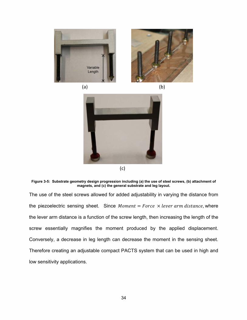
Figure 3-5: Substrate geometry design progression including (a) the use of steel screws, (b) attachment of magnets, and (c) the general substrate and leg layout.
The use of the steel screws allowed for added adjustability in varying the distance from
the piezoelectric sensing sheet. Since 𝑀𝑜𝑚𝑒𝑛𝑡 = 𝐹𝑜𝑟𝑐𝑒 × 𝑙𝑒𝑣𝑒𝑟 𝑎𝑟𝑚 𝑑𝑖𝑠𝑡𝑎𝑛𝑐𝑒, where
the lever arm distance is a function of the screw length, then increasing the length of the
screw essentially magnifies the moment produced by the applied displacement.
Conversely, a decrease in leg length can decrease the moment in the sensing sheet.
Therefore creating an adjustable compact PACTS system that can be used in high and
low sensitivity applications.
34
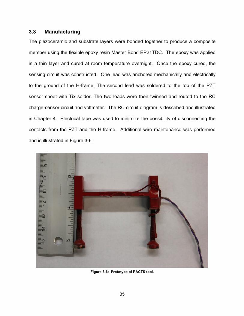
3.3 Manufacturing
The piezoceramic and substrate layers were bonded together to produce a composite
member using the flexible epoxy resin Master Bond EP21TDC. The epoxy was applied
in a thin layer and cured at room temperature overnight. Once the epoxy cured, the
sensing circuit was constructed. One lead was anchored mechanically and electrically
to the ground of the H-frame. The second lead was soldered to the top of the PZT
sensor sheet with Tix solder. The two leads were then twinned and routed to the RC
charge-sensor circuit and voltmeter. The RC circuit diagram is described and illustrated
in Chapter 4. Electrical tape was used to minimize the possibility of disconnecting the
contacts from the PZT and the H-frame. Additional wire maintenance was performed
and is illustrated in Figure 3-6.
Figure 3-6: Prototype of PACTS tool.
35
CHAPTER 4: PACTS MODELING
The PACTS tool design is composed of piezoceramic sensing material and a metallic
substrate bonded together. It is considered a composite system comprised of multiple
lamina, or layers. As a composite thin layer system the mechanical characteristics and
behavior can be analyzed using Classic Laminated Plate Theory (CLPT). This chapter
illustrates the modeling techniques used to analyze the PACTS system including closed
form solution of a sensing plate, and the PACTS tool design in addition to a finite
element analysis (FEA) of the PACTS system. An introduction to CLPT for a
nonhomogeneous isotropic laminate is followed by the CLPT approach used to analyze
the sensing capabilities of an isotropic PACTS system. The last section in this chapter
describes the finite element approach used to evaluate the sensitivity of the PACTS
system.
4.1 Closed Form Solution of Sensing Plates
4.1.1 Classic Laminate Plate Theory
CLPT uses the stress and deformation principles of mechanics-of-material as a
foundation to reduce three-dimensional elastic deformable body problems into two-
dimensional problems. Therefore, CLPT can be used to evaluate the behavior of
individual lamina, or layers, or various materials. This section will review the
mechanics-of-materials properties for individual lamina expressed as the kth lamina of
an N-layered laminate. Then, an investigation into the stress and strain variations
throughout the thickness of a laminate will be conducted. The laminate forces and
moments will be related to the strains and curvature of the laminate. The derivations of
isotropic behavior in this section are similar to the orthotropic solutions by Agarwal and
36

Jones (Agarwal and Bhagwan 2006; Jones 1975). Finally the sensing capabilities of a
piezoceramic unimorph sensing plate will be determined based on CLPT derivations.
The relationship between stress and strain for linear elastic materials can be evaluated
using the generalized Hooke’s Law, where σi are the stress components on a three-
dimensional cube in the x, y, and z coordinates (or 1, 2, and 3 direction), Cij is the
elastic stiffness matrix, and εj are the strain components as shown in Equation 4:1.
𝜎𝑖 = 𝐶𝑖𝑗 ∙ 𝜀𝑗 Equation 4:1
For an elastic material the stiffness matrix, Cij, is symmetric and contains 21
independent constants, therefore resulting in the following stress-strain relationship:
Equation 4:2
The sensing plate used in the PACTS tool design is comprised of three lamina including
a piezoceramic sheet, a layer of bond material, and the substrate material, aluminum.
Each material selected exhibits elastic and isotropic or quasi-isotropic behavior (Barrett
2013; Jones 1975). The following relationships exist between the elastic components of
isotropic materials within the elastic stiffness matrix:
𝐶11 = 𝐶22 = 𝐶33 𝐶12 = 𝐶13 = 𝐶23 𝐶44 = 𝐶55 = 𝐶66
Equation 4:3
σ1
σ2
σ3
τ23
τ31
τ12
→C11
C12
C13
C14
C15
C16
C12
C22
C23
C24
C25
C26
C13
C23
C33
C34
C35
C36
C14
C24
C34
C44
C45
C46
C15
C25
C35
C45
C55
C56
C16
C26
C36
C46
C56
C66
ε1
ε2
ε3
γ 23
γ 31
γ 12
→
⋅
C66C22 C23−
2
C11 C12−
2
37

Therefore, the generalized Hooke’s Law and the stiffness matrix becomes
Equation 4:4
In terms of the compliance matrix, S, or the inverse of the stress-strain relationship, the
strain-stress relation is as follows:
𝜀𝑖 = 𝑆𝑖𝑗 ∙ 𝜎𝑗 Equation 4:5
Equation 4:6
In accordance with CLPT, the laminate will be loaded under plane-stress conditions
within the 1-2 (x-y) plane of the composite. Therefore, all out of plane stresses will be
zero and
Equation 4:7
σ1
σ2
σ3
τ23
τ31
τ12
→C11
C12
C12
0
0
0
C12
C11
C12
0
0
0
C12
C12
C11
0
0
0
0
0
0
C11 C12−
2
0
0
0
0
0
0
C11 C12−
2
0
0
0
0
0
0
C11 C12−
2
ε1
ε2
ε3
γ 23
γ 31
γ12
→
⋅
ε1
ε2
ε3
γ 23
γ 31
γ 12
→S11
S12
S12
0
0
0
S12
S11
S12
0
0
0
S12
S12
S11
0
0
0
0
0
0
2 S11 S12−( )⋅
0
0
0
0
0
0
2 S11 S12−( )0
0
0
0
0
0
2 S11 S12−( )
σ1
σ2
σ3
τ23
τ31
τ12
→
⋅
𝜎3 = 𝜏23 = 𝜏13 = 0
38

For the plane-stress state, the generalized Hooke’s law reduces the stiffness matrix, C,
and the compliance matrix, S, from a 6 x 6 matrix to a 3 x 3 as shown in Figure 4-1 and
Figure 4-2.
Figure 4-1: Reduction of stiffness matrix, C, for an isotropic material under plane-stress conditions.
Figure 4-2: Reduction of compliance matrix, S, for an isotropic material under plane-stress conditions.
The strain-stress relations for an isotropic material under plane stress conditions using
the reduced compliance matrix, S, is as follows:
Equation 4:8
ε1
ε2
γ 12
→S11
S12
0
S12
S11
0
0
0
S66
σ1
σ2
τ12
→
⋅
39
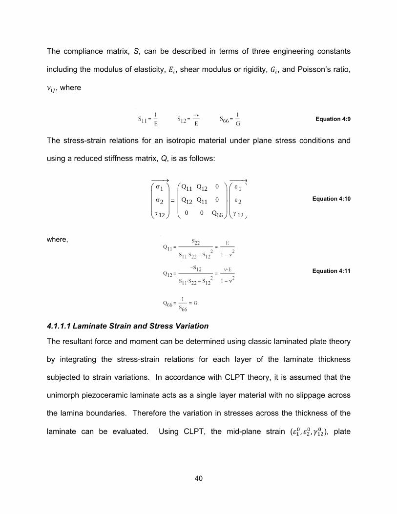
The compliance matrix, S, can be described in terms of three engineering constants
including the modulus of elasticity, 𝐸𝑖, shear modulus or rigidity, 𝐺𝑖, and Poisson’s ratio,
𝜈𝑖𝑗, where
Equation 4:9
The stress-strain relations for an isotropic material under plane stress conditions and
using a reduced stiffness matrix, Q, is as follows:
Equation 4:10
where,
Equation 4:11
4.1.1.1 Laminate Strain and Stress Variation
The resultant force and moment can be determined using classic laminated plate theory
by integrating the stress-strain relations for each layer of the laminate thickness
subjected to strain variations. In accordance with CLPT theory, it is assumed that the
unimorph piezoceramic laminate acts as a single layer material with no slippage across
the lamina boundaries. Therefore the variation in stresses across the thickness of the
laminate can be evaluated. Using CLPT, the mid-plane strain (𝜀10, 𝜀20, 𝛾120 ), plate
σ1
σ2
τ12
→Q11
Q12
0
Q12
Q11
0
0
0
Q66
ε1
ε2
γ 12
→
⋅
40

curvature (𝜅1, 𝜅2, 𝜅12), and the distance from mid-plane of the laminate, z, can be used
to determine strain at any point in a laminate using Equation 4:12.
Equation 4:12
Substitution of the through thickness strain variations (Equation 4:12) into Equation 4:10
yields the stresses in a specified layer in terms of the laminate middle-surface strains
and curvatures as
Equation 4:13
4.1.1.2 Laminate Forces and Moments
Resultant in-plane forces and moments (Figure 4-3) of a basic laminate geometry of an
N-Layered Laminate (Figure 4-4) can be determined using the stress and strain
variations presented in the section 4.1.1.1. Resultant forces Nij, are per unit width of the
laminate cross section. Similarly, the resultant moments, Mij, are per unit width of the
laminate.
Figure 4-3: In-Plane Forces, N, and Moments, M, on a flat surface.
ε1
ε2
γ 12
→ε1
0
ε20
γ 120
→
z
κ1
κ2
κ12
→
⋅+
σ1
σ2
τ12
→Q11
Q12
0
Q12
Q22
0
0
0
Q66
k
ε10
ε20
γ 120
z
κ1
κ2
κ12
+
→
⋅
41

Figure 4-4: Geometry of N-Layered Laminate (Jones 1975).
Since stresses within the laminate vary from lamina to lamina, the resultant forces and
moments acting on the laminate are determined by integration of the corresponding
stress through the laminate thickness. Equation 4:14 displays the resultant force in
units of force per unit length for the kth lamina of the general N-layered laminate (Figure
4-4).
Equation 4:14
Rearranging Equation 4:14 and substituting in Equation 4:13, the laminate forces
become
Equation 4:15
N11
N22
N12
→
t−
2
t
2
z
σ1
σ2
τ12
→⌠⌡
d
1
N
k
zk 1−
zk
z
σ1
σ2
τ12
k
→⌠⌡
d∑=
N11
N22
N12
→
1
N
k
Q11
Q12
0
Q12
Q22
0
0
0
Q66
k
∑=
zk 1−
zk
z
ε10
ε20
γ 120
→⌠⌡
d
zk 1−
zk
z
κ1
κ2
κ12
→
z⋅
⌠⌡
d+
⋅
42

Equation 4:16 displays the resultant moment in units of moment per length. Moment is
calculated by integrating the through thickness of the corresponding stress times the
moment arm with respect to the mid-plane of the laminate.
Equation 4:16
Rearranging Equation 4:16 and substituting in Equation 4:13, the laminate moments
becomes
Equation 4:17
Since 𝜀10, 𝜀20, 𝛾120 , and plate curvature are functions of the mid-plane and not of the plate
thickness, z, equations of force and moment per unit length can be rewritten in a
simplified form as
Equation 4:18
and
M11
M22
M12
→
t−
2
t
2
z
σ1
σ2
τ12
→
z⋅
⌠⌡
d
1
N
k
zk 1−
zk
z
σ1
σ2
τ12
k
→
z⋅
⌠⌡
d∑=
M11
M22
M12
→
1
N
k
Q11
Q12
0
Q12
Q22
0
0
0
Q66
k
∑=
zk 1−
zk
z
ε10
ε20
γ 120
→
z⋅
⌠⌡
d
zk 1−
zk
z
κ1
κ2
κ12
→
z2⋅
⌠⌡
d+
⋅
N11
N22
N12
→A11
A12
A16
A12
A22
A26
A16
A26
A66
ε10
ε20
γ 120
→
⋅
B11
B12
B16
B12
B22
B26
B16
B26
B66
κ1
κ2
κ12
→
⋅+
43

Equation 4:19
where,
Equation 4:20
The constitutive equation for the thin laminated plate includes Matrix A, the extensional
stiffness matrix which relates the resultant force per unit length to the mid-plane strains.
Matrix B is the coupling stiffness matrix that represents coupling behavior between
bending and the extension of the laminate. Matrix D is the bending stiffness matrix that
relates the resultant moment per length to the mid-plane plate curvatures of the
laminate. The compact notation of the total plate equation is presented in Equation
4:21.
Equation 4:21
4.1.1.3 Sensing Plate Systems
The unimorph laminate composed of piezoelectric material bonded to a structural
substrate subjected to bending is illustrated in Figure 4-5. The resulting strain in the
unimorph due to bending results in a charge change within the piezoceramic layer. The
M11
M22
M12
→B11
B12
B16
B12
B22
B26
B16
B26
B66
ε10
ε20
γ 120
→
⋅
D11
D12
D16
D12
D22
D26
D16
D26
D66
κ1
κ2
κ12
→
⋅+
Aij1
N
k
Qij( )
kzk zk 1−−( )
∑
=
Bij12
1
N
k
Qij( )
kzk
2 zk 1−( )2−
∑
=
Dij13
1
N
k
Qij( )
kzk
3 zk 1−( )3−
∑
=
N
M
→A
B
B
D
L
ε0
κ
→
⋅
44

charge generated in the piezoceramic layer is proportional to the strain (and strain times
rate of change) within the PZT layer.
Figure 4-5: Piezoelectric unimorph sensor.
Due to the bending action of the unimorph illustrated in Figure 4-5, the torsionally
induced shear and twist are negligible therefore reducing the total plate equation
(Equation 4:21) from a 6 x 6 to a 4 x 4 matrix as follows:
Equation 4:22
Where the laminate ABBD matrix is the summation of the ABBD matrix for each
lamina’s ABBD
A11
A12
B11
B12
A12
A22
B12
B22
B11
B12
D11
D12
B12
B22
D12
D22
L
ε11
ε22
κ11
κ22
→
⋅
N11
N22
M11
M22
→
A
B
B
D
L
A
B
B
D
p
A
B
B
D
b
+A
B
B
D
s
+
45

4.2 Closed Form Solution of the PACTS Tool
As described in Chapter 3, the PACTS tool is composed of a piezoceramic layer
bonded to the web of an H-shaped aluminum beam. The analysis of the PACTS tool
was conducted based on the CLPT and sensor analysis that was derived in Chapter 4.
In addition to the engineering constants including the modulus of elasticity, 𝐸𝑖, shear
modulus or rigidity, 𝐺𝑖, and Poisson’s ratio, 𝜈𝑖𝑗, used in CLPT, additional geometric
variables were investigated in analyzing the sensitivity of the PACTS tool (Figure 4-6).
The sensing capabilities of the PACTS system were analyzed by investigating the strain
within the PZT layer, where the voltage sensed, Vsensing, resulting from the strain and
displacement of the composite is proportional to the strain in the longitudinal direction of
the piezoelectric layer, ɛ11, and the thickness of the piezoceramic layer, tp. Thus:
𝑉𝑠𝑒𝑛𝑠𝑖𝑛𝑔 ∝ 𝜀𝑝 × 𝑡𝑝 Equation 4:23
Figure 4-6: PACTS tool diagram and variables used in CLPT analysis
The laminate force and moment based on CLPT is similar to those outlined in Equation
4:22; however, due to the shape of the PACTS tool and the large constraint at the tool
flanges, the beam or piezoceramic layer only bends in the longitudinal direction, x. This
46

bending action along the x-direction allows for the approximation that the force and
moment in the y-direction equal zero (𝑁22 = 0 𝑎𝑛𝑑 𝑀22 = 0). These boundary
conditions reduce the stress-strain relationship in Equation 4:22 to a 2 x 2 stiffness
matrix as follows:
Equation 4:24
Based on the geometry of the PACTS tool, the normal force per unit length, N11, can be
represented as a function of the horizontal force, FH, induced by the crack mouth
opening of the material per unit width, W, of the tool. Similarly, the moment per unit
length, M11, can be represented as the normal force per unit length multiplied by the
moment arm. The moment arm of the PACTS tool is the distance from the center line of
the tool to the contact surface of the material being detected or DFH. Therefore the force
and moment can be represented as follows:
Equation 4:25
Substitution of Equation 4:25 into Equation 4:24, yields
Equation 4:26
A11
B11
B11
D11
L
ε11
k11
→
⋅N11
M11
→
N11
M11
→ FHW
FH DFH⋅
W
→
A11
B11
B11
D11
L
ε11
k11
→
⋅
FHW
FH DFH⋅
W
47
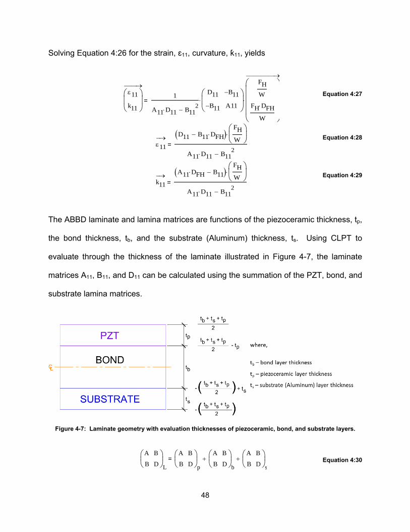
Solving Equation 4:26 for the strain, ɛ11, curvature, ƙ11, yields
Equation 4:27
Equation 4:28
Equation 4:29
The ABBD laminate and lamina matrices are functions of the piezoceramic thickness, tp,
the bond thickness, tb, and the substrate (Aluminum) thickness, ts. Using CLPT to
evaluate through the thickness of the laminate illustrated in Figure 4-7, the laminate
matrices A11, B11, and D11 can be calculated using the summation of the PZT, bond, and
substrate lamina matrices.
Figure 4-7: Laminate geometry with evaluation thicknesses of piezoceramic, bond, and substrate layers.
Equation 4:30
ε11
k11
→
1
A11 D11⋅ B112
−
D11
B11−
B11−
A11
⋅
FHW
FH DFH⋅
W
→
⋅
ε11→ D11 B11 DFH⋅−( )
FHW
⋅
A11 D11⋅ B112
−
k11→ A11 DFH⋅ B11−( )
FHW
⋅
A11 D11⋅ B112
−
A
B
B
D
L
A
B
B
D
p
A
B
B
D
b
+A
B
B
D
s
+
48

where,
Ep = PZT Modulus Elasticity
Eb = Bond Material Modulus of Elasticity
Es = Substrate (Aluminum) Modulus of Elasticity
Solving Equation 4:27 for the strain in the PZT layer, ɛp, yields
ɛ𝑝 = ɛ11 ± �𝑡𝑏 + 𝑡𝑠
2� ƙ11 Equation 4:31
| | | | | | |
| | | | | | |
==>
| | | | | | |
| | | | | | |
==>
| | | | | | |
| | | | | | |
==>
A11 A11p A11b+ A11s+
A11p Eptb ts+ tp−
2
tb ts+ tp+
2z1
⌠⌡
d⋅ A11b Ebtb ts+ tp+
2− ts+
tb ts+ tp−
2z1
⌠⌡
d⋅ A11s Estb ts+ tp+
2−
tb ts+ tp+
2− ts+
z1
⌠⌡
d⋅
B11 B11p B11b+ B11s+
B11p Eptb ts+ tp−
2
tb ts+ tp+
2zz
⌠⌡
d⋅ B11b Ebtb ts+ tp+
2− ts+
tb ts+ tp−
2zz
⌠⌡
d⋅ B11s Estb ts+ tp+
2−
tb ts+ tp+
2− ts+
zz
⌠⌡
d⋅
D11 D11p D11b+ D11s+
D11p Eptb ts+ tp−
2
tb ts+ tp+
2zz2
⌠⌡
d⋅ D11b Ebtb ts+ tp+
2− ts+
tb ts+ tp−
2zz2
⌠⌡
d⋅ D11s Estb ts+ tp+
2−
tb ts+ tp+
2− ts+
zz2⌠⌡
d⋅
49

The sensitivity of the PACTS tool as a function of the PZT thickness and longitudinal
strain can be found by substituting Equation 4:31 into the sensitivity equation (Equation
4:23).
𝑉𝑝𝑖𝑒𝑧𝑜 ∝ �ɛ11 ± �𝑡𝑏 + 𝑡𝑠
2� ƙ11� ∙ 𝑔31𝑡𝑝 Equation 4:32
𝑉𝑠𝑒𝑛𝑠𝑒𝑑 ∝ 𝑓 ∙ 𝑅 �ɛ11 ± �𝑡𝑏 + 𝑡𝑠
2� ƙ11� ∙
𝑔31𝑡𝑝𝐶𝑞−𝑠𝑡𝑜𝑟𝑒
Equation 4:33
Where
g31 – the strain developed per applied charge density, where the stress is applied in the
X-direction (axis 1) and the electrodes are applied perpendicular to the Z-axis (axis 3)
Cq-store – the stored charge in the capacitor within the circuit (including total circuit capacitance)
R – Resistance
f – Frequency of excitation
4.2.1 Generalized Solution
So as to give the reader a fundamental feel for the most important driving parameters
and relationships, the PACTS system can be greatly simplified:
Since the bond layer stiffness is significantly less than the PZT and substrate, the
PACTS system sensitivity is governed by the PZT and substrate layers. Therefore
sensitivity equations can be determined using a two layer laminate (Figure 4-8).
50

Figure 4-8: Two layer laminate of the driving parameters of the PACTS tool.
Remembering Hooke’s Law where the resultant forces, where
Equation 4:34
or
Equation 4:35
Considering shear and twist terms trend towards zero and expanding Equation 4:35
yields the following:
Equation 4:36
Assuming isotropic behavior of the laminate, then
𝐴11 ≡ 𝐴22 𝐵11 ≡ 𝐵22 𝐷11 ≡ 𝐷22
and
F k ∆x⋅
N
M
→A
B
B
D
ε0
κ
→
⋅
N11
N22
M11
M22
→A11
A12
B11
B12
A12
A22
B12
B22
B11
B12
D11
D12
B12
B22
D12
D22
ε110
ε220
k11
k22
→
⋅
51

Equation 4:37
Assuming the mid-plane strain in the PZT, ɛpiezo, is dominated by moments, then
𝜀110 ≅ 𝜀220 ≅ 0
Assuming the H-frame generates enough lateral stiffness where
𝜀220 ≅ 0
then Equation 4:37 reduces to a scalar, where
Equation 4:38
Solving for curvature, ƙ11
Equation 4:39
From Equation 4:25, the moment per unit width of the PACTS tool, M11 can be
substituted into Equation 4:39, then curvature, κ11, can be expressed in terms of FH,
DFH, and W as follows:
Equation 4:40
As previously stated, the mid-plane strain of the laminate is approximately zero
therefore, translating the curvature, ƙ11, solution into the mid-plane strain in the PZT,
N11
N22
M11
M22
→A11
A12
B11
B12
A12
A11
B12
B11
B11
B12
D11
D12
B12
B11
D12
D11
ε110
ε220
k11
k22
→
⋅
M11( )→
D11( ) κ11( )→
⋅
M11 D11 κ11⋅
κ11M11D11
κ11FH DFH⋅
W D11⋅
52

ɛpiezo, can be done using small angle theory and evaluating the thickness illustrated in
Figure 4-9.
Figure 4-9: PZT and substrate dominated laminate.
Where,
Equation 4:41
And
𝜀𝑝𝑖𝑒𝑧𝑜 =
𝑡𝑠2�
𝑙𝑜∙ 𝛼 Equation 4:42
Substitution of Equation 4:41 into Equation 4:42, assuming that the stiffness of the
piezoceramic is roughly equal to that of the substrate, the following expression holds
true:
𝜀𝑝𝑖𝑒𝑧𝑜~𝑡𝑠2∙ ƙ11 Equation 4:43
α κdegrees
in
lo in( )⋅
53

If
𝑉𝑝𝑖𝑒𝑧𝑜 ∝ ɛ𝑝𝑖𝑒𝑧𝑜 ∙ 𝑔31 ∙ 𝑡𝑝 Equation 4:44
Then substituting Equation 4:43 into Equation 4:44 yields
𝑉𝑝𝑖𝑒𝑧𝑜 ∝𝑡𝑠2∙ 𝜅11 ∙ 𝑔31 ∙ 𝑡𝑝 Equation 4:45
The resulting voltage in the PZT layer can be expressed in terms of the PACTS
geometry, by substituting the curvature, κ11, expression (Equation 4:40) into Equation
4:45. Therefore,
𝑉𝑝𝑖𝑒𝑧𝑜 ∝𝑡𝑠 ∙ 𝑡𝑝
2∙ 𝑔31 ∙ �
𝐹𝐻 ∙ 𝐷𝐹𝐻𝐷11 ∙ 𝑊
� Equation 4:46
The circuit designed in order to document the sensed voltage of the PACTS systems is
illustrated in Figure 4-10. The circuit is directly connected to the PZT layer of the
PACTS tool, and includes a resistor and capacitor.
Figure 4-10: PACTS tool test RC charging circuit diagram.
Therefore the voltage read from the multimeter, or Vsensed, can be evaluated using, the
voltage in the PZT, Vpiezo, the frequency, 𝑓, and time as shown in Equation 4:47.
54

𝑉𝑠𝑒𝑛𝑠𝑒𝑑 ∝𝑡𝑠 ∙ 𝑡𝑝 ∙ 𝑔31 ∙ �
𝐹𝐻 ∙ 𝐷𝐹𝐻𝐷11 ∙ 𝑊
� ∙ 𝑓 ∗ 𝑡𝑖𝑚𝑒
𝐶𝑞−𝑠𝑡𝑜𝑟𝑒𝑑 Equation 4:47
Initially, as time, t, increases the voltage sensed increases linearly. However,
eventually, the voltage level will reach a point where the shunting resistor allows enough
current to leak through it and the voltage sensed trends towards an asymptotic value as
shown in Figure 4-11. This research limited its application to the linear range, therefore,
non-linear sensing is outside of the scope of this dissertation.
Figure 4-11: General relationship of sensed Voltage, Vs and time, t of RC charging circuit.
4.3 Finite Element Analysis
A detailed analytical investigation was conducted on the basic H-shape design of the
PACTS system using finite element (FE) modeling software ABAQUS 6.12-3. The two-
dimension linear elastic model was composed of three main parts: H-beam, bond layer,
and PZT layer. Due to the doubly symmetric nature of H-section members, only half of
the sensor shape (Figure 4-12) was modeled therefore simplifying the size of the finite
55

element model and reducing analysis time requirements of the program. The modeled
parts were connected using surface-to-surface tie constraints and each part of the
model had independent material properties. The Young’s moduli were taken as 69 GPa
[10,000 ksi], 62 GPa [9,000 ksi], and 1.97 GPa [286 ksi] for aluminum substrate, PZT,
and bond material, respectively. The material properties used for the FE model and
Closed Form Solution are located in Appendix A.
Figure 4-12: FE model of PACTS tool layout with applied unit force
The model was developed to determine the maximum longitudinal strain, ɛ11, in the mid-
plane of the PZT layer. In accordance with the sensing capabilities of the PZT
materials, the voltage sensed by a piezoceramic sensor is proportional to the mid-plane
strain of the PZT layer times the PZT layer thickness, tp. In order to generalize the
56
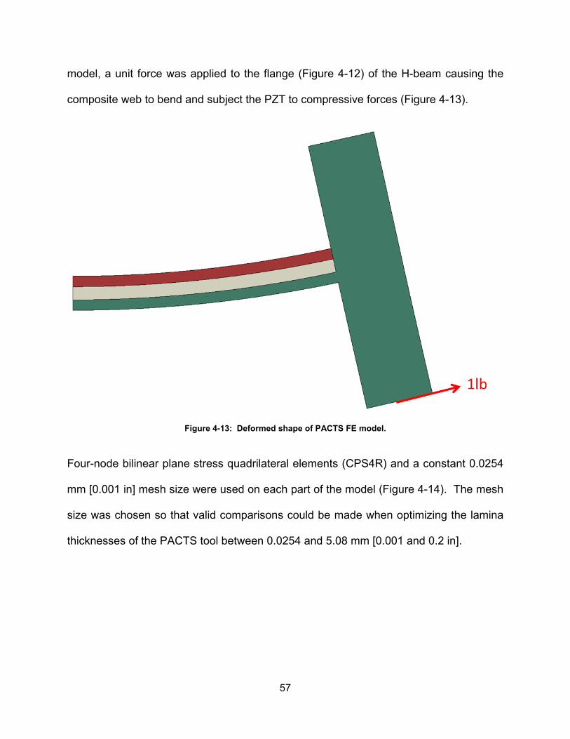
model, a unit force was applied to the flange (Figure 4-12) of the H-beam causing the
composite web to bend and subject the PZT to compressive forces (Figure 4-13).
Figure 4-13: Deformed shape of PACTS FE model.
Four-node bilinear plane stress quadrilateral elements (CPS4R) and a constant 0.0254
mm [0.001 in] mesh size were used on each part of the model (Figure 4-14). The mesh
size was chosen so that valid comparisons could be made when optimizing the lamina
thicknesses of the PACTS tool between 0.0254 and 5.08 mm [0.001 and 0.2 in].
57

Figure 4-14: Mesh size 0.0254 mm [0.001 in] in each layer of the FE model.
Since the model is symmetric along the X-axis, a symmetry boundary condition was
used. The XSYMM boundary condition of the two-dimension model restrains
displacement in the X-direction and rotation about the Y and Z-axis (Figure 4-15).
Figure 4-15: Symmetric boundary condition used in the Abaqus FE model of the PACTS geometry.
58

4.4 Summary
The results of the FE and CLPT theory indicated that the sensitivity of the PACTS tool
was dependent on the geometry of the substrate, PZT, and bond layer of the system.
The methods used in the modeling of the PACTS system were instrumental in
determining the optimum design geometry for the prototype used in the experimental
analysis of the tool sensitivity. The design of the PACTS was specifically oriented such
that the PZT layer remained in compression when subjected to an applied load or
displacement. Based on the FE analysis results, the initial design assumption was
validated and the PACTS tool will operate below the ultimate compressive stress of the
PZT.
59

CHAPTER 5: PACTS OPTIMIZATION This chapter investigates the effects of the laminate material property on the sensitivity
of the PACTS tool in order to optimize the sensing capabilities of the sensing tool. This
analysis was done using the FE software and CLPT mentioned in Chapter 4. The
resulting sensitivity or charge generated, by the PZT was plotted against the thickness
of substrate.
5.1 Finite Element Results
Using the FE linear elastic model of the aluminum substrate, bond, and PZT layers
described Chapter 3, each layer thickness was varied and the longitudinal mid-plane
PZT layer strain values were analyzed. Based on the model geometry, loading, and
boundary conditions chosen, the optimization process required a parametric study that
varied material thickness ranges for each layer of the laminate. PZT thicknesses (tp)
ranges investigated were from 0.254 mm [0.010 in] to 2.54 mm [0.100 in]; bond
thicknesses (tb) between 0.0254 mm [0.001 in] and 1.016 mm [0.040 in]; and the
aluminum substrate thicknesses (ts) were between 1.016 mm [0.040 in] to 5.08 mm
[0.200 in]. The specific thicknesses evaluated for each layer are presented in Table
5-1. The substrate thickness study was conducted on additional thickness sizes due to
the adjustability of the H-shaped web that was initially fabricated to 5.08 mm [0.200 in].
Modifications to the standard shape could be made using a mill scale allowing more
adjustability to the design. Bond thickness range was larger due to the application and
shrinkage variations that can occur during the manufacturing and curing process. A
total of 175 finite element models were created for this parametric study. From these
60

models, the effects of varying the substrate web, bond layer, and PZT thicknesses were
analyzed and an optimal shape was selected to use in the Proof of Concept testing.
Table 5-1: Laminate layer thicknesses used in the FE models generated for the optimization study.
PZT Thickness, tp, mm [in]
Bond Thickness, tb mm [in]
Substrate Thickness, ts mm [in]
0.254 [0.010] 0.0254 [0.001] 1.016 [0.040]
0.508 [0.020] 1.27 [0.050] 1.27 [0.050]
1.016 [0.040] 2.54 [0.100] 1.905 [0.075]
2.032 [0.080] 5.08 [0.200] 2.54 [0.100]
2.54 [0.100] 6.35 [0.250] 3.175 [0.125]
- - 3.81 [0.150]
- - 5.08 [0.200]
From Chapter 4, it was determined that the voltage sensed in the PZT layer was
proportional to the change in strain in the mid-plane of the PZT times the PZT layer.
Therefore, the results presented in this section include the normalized charge generated
in the mid-plane of the PZT plotted against the thickness of the substrate web. Since
the laminate beam is in bending, it is assumed that the PZT is subjected to compression
loading; therefore, the resulting voltage sensed is negative. In all cases, the magnitude
of the charge generated and resulting maximum voltage sensed were used in the
comparison of the sensing capabilities of the PACTS tool. The strain data was selected
along the mid-plane path of the PZT layer in each model analyzed as illustrated in
Figure 5-1.
61
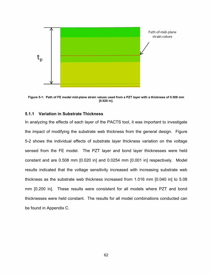
Figure 5-1: Path of FE model mid-plane strain values used from a PZT layer with a thickness of 0.508 mm [0.020 in].
5.1.1 Variation in Substrate Thickness
In analyzing the effects of each layer of the PACTS tool, it was important to investigate
the impact of modifying the substrate web thickness from the general design. Figure
5-2 shows the individual effects of substrate layer thickness variation on the voltage
sensed from the FE model. The PZT layer and bond layer thicknesses were held
constant and are 0.508 mm [0.020 in] and 0.0254 mm [0.001 in] respectively. Model
results indicated that the voltage sensitivity increased with increasing substrate web
thickness as the substrate web thickness increased from 1.016 mm [0.040 in] to 5.08
mm [0.200 in]. These results were consistent for all models where PZT and bond
thicknesses were held constant. The results for all model combinations conducted can
be found in Appendix C.
62

Figure 5-2: FE model results of PACTS voltage sensitivity as a function of the aluminum substrate thickness for a 0.508 mm [0.020 in] thick PZT layer and a 0.0254 mm [0.001 in] thick bond layer.
5.1.2 Variations in Bond Thickness
Bond thickness was found to be inversely related to the sensitivity of the PACTS tool.
Figure 5-3 illustrates the sensitivity for a 0.508 mm [0.020 in] PZT layer thickness,
where the bond thickness varied from 0.0254 mm [0.001 in] to 6.35 mm [0.25 in].
Results indicate that the sensitivity decreases with increasing bond layer thickness. As
the thickness of the bond layer increases, it appears that the effects of shear lag
significantly retard the sensing capabilities of the laminate. As the bond thickness
increases, more and more energy is imparted to shear deformations in the bond, which
means that less and less energy is imparted to the piezoelectric sensing material.
Therefore, the bond layer thickness should be minimized to increase sensitivity of the
0.040 0.080 0.120 0.160 0.200-1.2
-1.0
-0.8
-0.6
-0.4
-0.2
0.0
-30.48
-25.40
-20.32
-15.24
-10.16
-5.08
0.001.02 2.03 3.05 4.06 5.08
Aluminum Substrate Thickness, ts (in)
Norm
alized strain in Piezoelectric Element x tp (με *in) N
orm
aliz
ed st
rain
in P
iezo
elec
tric
Ele
men
t x t p
(με
*mm
) Aluminum Substrate Thickness, ts (mm)
63
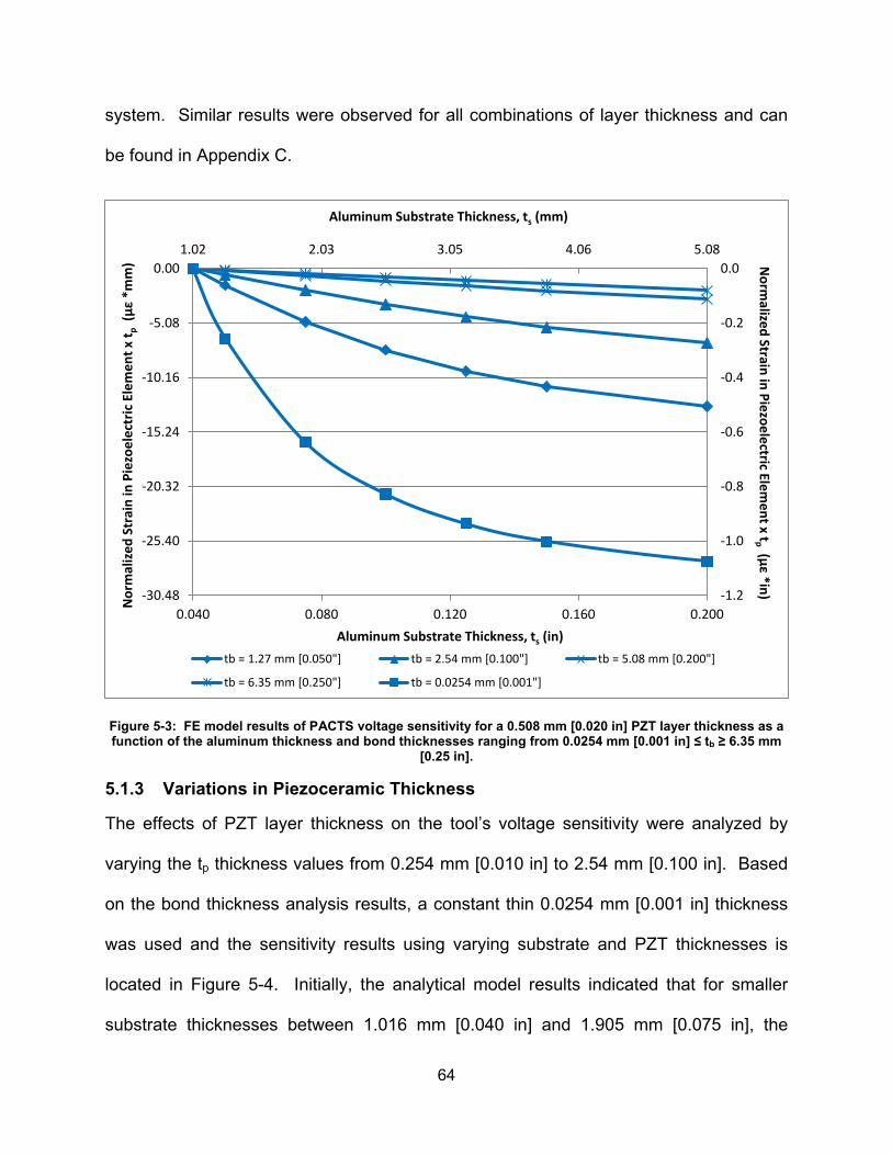
system. Similar results were observed for all combinations of layer thickness and can
be found in Appendix C.
Figure 5-3: FE model results of PACTS voltage sensitivity for a 0.508 mm [0.020 in] PZT layer thickness as a function of the aluminum thickness and bond thicknesses ranging from 0.0254 mm [0.001 in] ≤ tb ≥ 6.35 mm
[0.25 in].
5.1.3 Variations in Piezoceramic Thickness
The effects of PZT layer thickness on the tool’s voltage sensitivity were analyzed by
varying the tp thickness values from 0.254 mm [0.010 in] to 2.54 mm [0.100 in]. Based
on the bond thickness analysis results, a constant thin 0.0254 mm [0.001 in] thickness
was used and the sensitivity results using varying substrate and PZT thicknesses is
located in Figure 5-4. Initially, the analytical model results indicated that for smaller
substrate thicknesses between 1.016 mm [0.040 in] and 1.905 mm [0.075 in], the
0.040 0.080 0.120 0.160 0.200-1.2
-1.0
-0.8
-0.6
-0.4
-0.2
0.0
-30.48
-25.40
-20.32
-15.24
-10.16
-5.08
0.001.02 2.03 3.05 4.06 5.08
Aluminum Substrate Thickness, ts (in)
Norm
alized Strain in Piezoelectric Element x tp (με *in) N
orm
aliz
ed S
trai
n in
Pie
zoel
ectr
ic E
lem
ent x
t p (με
*mm
)
Aluminum Substrate Thickness, ts (mm)
tb = 1.27 mm [0.050"] tb = 2.54 mm [0.100"] tb = 5.08 mm [0.200"]
tb = 6.35 mm [0.250"] tb = 0.0254 mm [0.001"]
64

voltage sensitivity of the PACTS tool decreased with increasing PZT thickness.
However, at larger substrate thicknesses the 0.508 mm [0.020 in] thick PZT geometry
resulted in larger sensitivity results that increased with increasing aluminum substrate
thicknesses. From the figure and the model results, it was determined that for a thin
substrate thickness, in combination with thin bond thickness and large PZT thickness,
the neutral axis of the composite member shifts upward. Therefore, the mid-plane
strain in the PZT is under tensile loading conditions which resulted in positive sensitivity
values at ts = 1.27 mm [0.050 in], tb = 0.0254 mm [0.001 in], and tp = 2.54 mm [0.100 in].
However, as the substrate web thicknesses increase the PZT remains in compression;
therefore, the PZT sheets operate below the ultimate compressive strength of the
material.
65

Figure 5-4: FE model results of PACTS voltage sensitivity as a function of PZT layer thicknesses and
aluminum substrate thickness using a constant 0.0254 mm [0.001 in] bond layer thickness.
5.1.4 Summary of Results
The results for all 175 models were analzyed and compiled for comparison and are
presented in Figure 5-5. The results illustrate that generally smaller PZT thickness in
conjunction with a thin bond layer thickness will provide the most highly senstive results
for all substrate web thicknesses. However, at a substrate web thickness of
approximately 1.905 mm [0.075 in], the 0.508 mm [0.020 in] thick PZT layer begins to
out perform the thinner 0.254 mm [0.010 in] thickness.
0.040 0.080 0.120 0.160 0.200-1.2
-1
-0.8
-0.6
-0.4
-0.2
0
0.2
-30.48
-25.4
-20.32
-15.24
-10.16
-5.08
0
5.081.02 2.03 3.05 4.06 5.08
Aluminum Substrate Thickness, ts (in)
Norm
alized Strain in Piezoelectric Element x tp (με *in) N
orm
aliz
ed S
trai
n in
Pie
zoel
ectr
ic E
lem
ent x
t p (με
*mm
) Aluminum Substrate Thickness, ts (mm)
tp = 0.254mm [0.010"], tb = 0.0254mm [0.001"] tp = 0.508mm [0.020"], tb = 0.0254mm [0.001"]tp = 1.016mm [0.040"], tb = 0.0254mm [0.001"] tp = 2.032mm [0.080"], tb = 0.00254mm [0.001"]tp = 2.54mm [0.100"], tb = 0.0254mm [0.001"]
66

Figu
re 5
-5:
Para
met
ric a
naly
sis
of v
olta
ge s
ensi
tivity
of t
he P
AC
TS to
ol g
eom
etry
as
a fu
nctio
n of
PZT
, bon
d m
ater
ial,
and
alum
inum
sub
stra
te la
yer
thic
knes
ses.
0.04
00.
060
0.08
00.
100
0.12
00.
140
0.16
00.
180
0.20
0-1.2
-1-0.8
-0.6
-0.4
-0.2
0
-30.
48
-25.
4
-20.
32
-15.
24
-10.
16
-5.0
801.02
1.60
2.18
2.76
3.34
3.92
4.50
5.08
Alum
inum
Sub
stra
te T
hick
ness
, ts (
in)
Normalized Strain in Piezoelectric Element x tp (με *in)
Normalized Strain in Piezoelectric Element x tp (με *mm) Al
umin
um S
ubst
rate
Thi
ckne
ss, t
s (m
m)
tp =
0.2
54m
m [0
.010
"], tb
= 0
.025
4mm
[0.0
01"]
tp =
0.2
54m
m [0
.010
"], tb
= 1
.27m
m [0
.050
"]
tp=
0.25
4mm
[0.0
10"],
tb =
2.5
4mm
[0.1
00"]
tp =
0.2
54m
m [0
.010
"], tb
= 5
.08m
m [0
.200
"]
tp =
0.2
54m
m [0
.010
"], tb
= 6
.35m
m [0
.250
"]
tp =
0.5
08m
m [0
.020
"], tb
= 0
.025
4mm
[0.0
01"]
tp =
0.5
08m
m [0
.020
"], tb
= 1
.27m
m [0
.050
"]
tp =
0.5
08m
m [0
.020
"], tb
= 2
.54m
m [0
.100
"]
tp =
0.5
08m
m [0
.020
"], tb
= 5
.08m
m [0
.200
"]
tp =
0.5
08m
m [0
.020
"], tb
= 6
.35m
m [0
.250
"]
tp =
1.0
16m
m [0
.040
"], tb
= 0
.025
4mm
[0.0
01"]
tp =
1.0
16m
m [0
.040
"], tb
= 1
.27m
m [0
.050
"]
tp =
1.0
16m
m [0
.040
"], tb
= 2
.54m
m [0
.100
"]
tp =
1.0
16m
m [0
.040
"], tb
= 5
.08m
m [0
.200
"]
tp =
1.0
16m
m [0
.040
"], tb
= 6
.35m
m [0
.250
"]
tp =
2.0
32m
m [0
.080
"], tb
= 0
.002
54m
m [0
.001
"]
tp =
2.0
32m
m [0
.080
"], tb
= 1
.27m
m [0
.050
"]
tp =
2.0
32m
m [0
.080
"], tb
= 2
.54m
m [0
.100
"]
tp =
2.0
32m
m [0
.080
"], tb
= 5
.08m
m [0
.200
"]
tp =
2.0
32m
m [0
.080
"], tb
= 6
.35m
m [0
.250
"]
tp =
2.5
4mm
[0.1
00"],
tb =
0.0
254m
m [0
.001
"]
tp =
2.5
4mm
[0.1
00"],
tb =
1.2
7mm
[0.0
50"]
tp =
2.5
4mm
[0.1
00"],
tb =
2.5
4mm
[0.1
00"]
tp =
2.5
4mm
[0.1
00"],
tb =
5.0
8mm
[0.2
00"]
tp =
2.5
4mm
[0.1
00"],
tb =
6.3
5mm
[0.2
50"]
67

Based on the results of the parametric study, the PACTS tool geometry (Figure 5-6)
with a substrate thickness of 1.905 mm [0.075 in] and a PZT sheet of 0.508 mm [0.020
in] were selected and manufactured to conduct experimental testing on an artificial
crack. It was determined that the bond material thickness should be limited to
production ability and the manufacturer’s instruction. After manufacturing the optimized
geometry and adding the leg system, the resulting PACTS tool used in the the proof of
concept testing weighed 20 g [0.044 lbs.]
Figure 5-6: Optimized PACTS tool geometry selected for the proof of concept testing.
68

CHAPTER 6: PACTS PROOF OF CONCEPT The primary objective of this chapter is to demonstrate the feasibility of the proposed
piezoelectric sensor concept. This was carried out using the PACTS tool under
laboratory conditions and analyzing the energy harvested by the sensor on an artificial
crack and an acrylic compact tension specimen subjected to dynamic loading. This
chapter identifies the test methods used and verifies the initial assumptions and
hypothesis of this research. The results of the FE modeling and experimental test
methods used for the PACTS tool with the optimal geometry determined in Chapter 5
are presented in this section.
6.1 Finite Element Analysis Results
FE results for the optimal PZT and substrate layer thickness of 0.508 mm [0.020 in] and
1.905 mm [0.075 in] respectively validate the assumption that the PZT layer would be
subjected to compressive strains, due to the deformation of the PACTS geometry when
loaded. The FE results are shown in Figure 6-1. The deformation scale for the figure is
400 and the strain data shown in the legend were selected to emphasize the
compressive longitudinal strain values of the tool geometry.
69

Figure 6-1: FE longitudinal mid-plane strain results for the selected PACTS tool geometry, where tp = 0.508
mm [0.020 in], tb = 0.0254 mm [0.001 in], and ts = 1.905 mm [0.075 in], verifying that the PZT layer is in compression under testing conditions for the selected geometry.
6.2 Artificial Crack System Experiment
An Artificial Crack System (ACS) was fabricated in order to investigate the sensitivity of
the PACTS tool and its ability to detect an active crack. The ACS provided a crack
length of 300 mm [11.8 in] that was used to analyze the effectiveness of the PACTS
tool. The artificial crack was composed of two steel plates including a main post and a
swing arm. The two steel plates rotate about a hinge point that functioned similarly to a
crack tip. A specified displacement can be applied to the apparatus that allows the
swing arm surface to separate from the main post. This separation from the main post
results in an edge crack under fracture Mode I opening that could be spanned by the
PACTS tool. Fabrication drawings for the ACS are located in Appendix D.
70
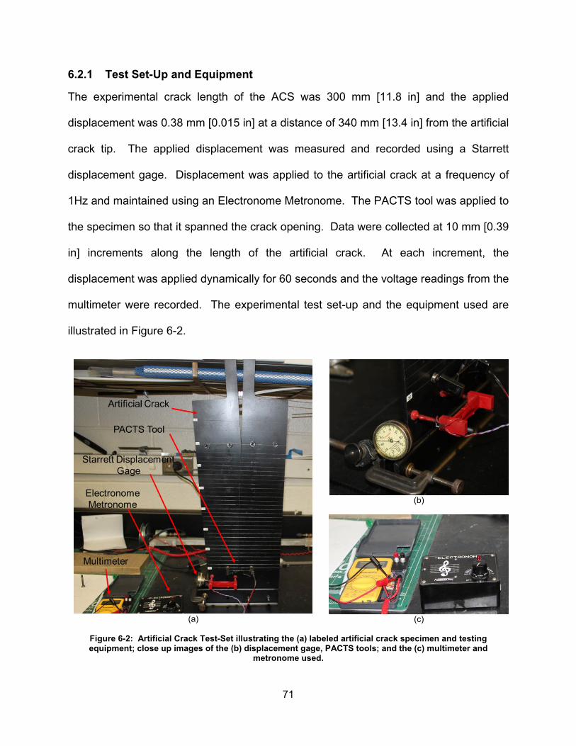
6.2.1 Test Set-Up and Equipment
The experimental crack length of the ACS was 300 mm [11.8 in] and the applied
displacement was 0.38 mm [0.015 in] at a distance of 340 mm [13.4 in] from the artificial
crack tip. The applied displacement was measured and recorded using a Starrett
displacement gage. Displacement was applied to the artificial crack at a frequency of
1Hz and maintained using an Electronome Metronome. The PACTS tool was applied to
the specimen so that it spanned the crack opening. Data were collected at 10 mm [0.39
in] increments along the length of the artificial crack. At each increment, the
displacement was applied dynamically for 60 seconds and the voltage readings from the
multimeter were recorded. The experimental test set-up and the equipment used are
illustrated in Figure 6-2.
(a)
(b)
(c)
Figure 6-2: Artificial Crack Test-Set illustrating the (a) labeled artificial crack specimen and testing equipment; close up images of the (b) displacement gage, PACTS tools; and the (c) multimeter and
metronome used.
71

6.2.2 Test Results
The results of the ACS test indicate that the sensor is actively detecting the presence of
an active crack. Voltage reading values increased with increasing distance away from
the artificial crack tip. These results correlate to geometric fracture principles where
crack opening displacement increases linearly as the distance from the crack tip
increases. However, at a distance less than 50 mm [2.0 in] from the artificial crack tip
the results indicate non-linear behavior. The results presented are similar to issues
identifying crack tips in real structures where areas near the crack tip typically include
regions of plastic deformation outside of the linear elastic analysis region under
consideration within this research. The non-linearity of ACS results could be due to
fabrication and design of the hinge point. However based on the linear region of the
data, the crack tip could be extrapolated using the slope of the linear region to the
location of the artificial.
72

Figure 6-3: Voltage reading at 60 seconds using a 1000 μF capacitor and 50kΩ of resistance in the PZT
sensing circuit when a 0.381mm [0.0150 in] displacement (measured at 340 mm [13.4 in] from the artificial crack tip) is applied at a frequency of 1Hz.
6.2.3 Summary
The PACTS tool successfully detected the presence of an active crack. The sensitivity
capabilities of the PACTS tool accurately detected the presence of crack opening
displacement along the length of the artificial crack up to 0.056 mm [0.0022 in]. At a
location of 50 mm [2.0 in] from the artificial crack tip, a change in slope within linear
trend of PACTS voltage sensitivity was observed. Using only the crack opening linear
trend (COLT) data, the crack tip position could be effectively determined. The results
also suggest that the location of the crack tip could be determined based on the slope
change of the PACTS voltage data.
0 2 4 6 8 10
0
2
4
6
8
10
12
0 50 100 150 200 250 300
Distance from Artificial Crack Tip (in) Vo
ltage
Rea
ding
at 6
0 se
c. (m
V)
Distance from Artificial Crack Tip (mm)
73

6.3 Crack Tip Identification and Location
After successfully using the PACTS system to identify active crack opening
displacements on the steel ACS, the tool was used to evaluate the ability to identify the
crack tip in an acrylic specimen. Therefore, a 38.1 mm [1.5 in] thick acrylic sheet was
cut to the Compact Tension (CT) specimen requirements as per ASTM E399 (2012).
The dimensions and straight through notch crack size of the acrylic CT specimen is
illustrated in Figure 6-4 and the material characteristics of the acrylic specimen are
described in Appendix A.
Figure 6-4: Acrylic compact tension specimen geometry used for the crack tip identification testing.
74

6.3.1 Test Set-Up and Equipment
The CT specimen was marked in 1 cm [0.39 in] increments from the crack tip, up to 20
mm [0.79 in] ahead of the crack tip and 50 mm [1.97 in] behind the crack tip as
illustrated in Figure 6-5 (a). A 1.5 m [5 ft] long aluminum beam was attached to the
surface of the CT specimen with a load attached to the cantilever end as shown in
Figure 6-5 (b). The CT specimen was dynamically loaded at 2.2 Hz. The PACTS tool
was placed across the crack at 10 mm [0.39 in] increments along the CT specimen
while it was loaded dynamically for 60 seconds at each increment, similarly to the ACS
test.
Figure 6-5: (a) Acrylic test specimen used in the in the (b) crack tip boundary identification experiment.
6.3.2 Results
PACTS tool testing was conducted up to 20 mm [0.79 in] ahead of the crack tip and 50
mm [1.97 in] behind the crack tip. The voltage readings from the PACTS tool after 60
seconds of cycling are shown in Figure 6-6. As theorized and shown using the ACS
test set-up, the voltage sensed results increase with increasing distance from the crack
tip. The voltage sensed continued to decrease ahead of the crack tip as it approached
an area of zero displacement within the material. Results also indicate a region of non-
75

linear response near the crack tip of the specimen. These results confirm the test data
acquired using the ACS test setup.
Figure 6-6: Voltage readings taken at 10 mm [0.39 in] increments along the test specimen over 60 seconds at
a frequency of 2.2 Hz
Based on the test results, a linear relationship exists between the voltage reading and
the distance behind and ahead of the crack tip (Figure 6-7). Similarly to the ACS
results, non-linear sensing is evident near the crack tip region. Using a COLT analysis,
the crack tip position could be located within 2.72 mm [0.107 in]. However, it is
hypothesized that the location of the crack tip can be estimated using the change in
slope from the linear region of the test data. In order to determine the location of the
crack tip of the specimen, additional analytical calculations were required.
-0.79 -0.29 0.21 0.71 1.21 1.71
0
0.5
1
1.5
2
2.5
-20 -10 0 10 20 30 40 50
Distance from Crack Tip (in)
Volta
ge R
eadi
ng a
t 60
sec.
(mV)
Distance from Crack Tip (mm)
76

Figure 6-7: Voltage reading taken over 60 seconds at frequency of 2.2 Hz with trend lines added to the linear
regions behind and ahead of the crack tip.
6.3.3 Crack tip location determination
To identify the crack tip location based on the change in slope of the linear data, it was
important to identify a line tangent to the non-linear region, between 0 mm [0 in] and 20
mm [0.79 in], that also includes the location of the crack tip at (0, 0). From the test data
and the equation of the non-linear region, it was determined that a line through (0, 0)
that is tangent to the non-linear portion at 14.8 mm [0.58 in] and 0.583 mV had a slope
of 0.0339 as shown in Figure 6-8.
y = 0.0501x - 0.1361
y = 0.0127x + 0.323
-0.79 -0.29 0.21 0.71 1.21 1.71
-0.5
0
0.5
1
1.5
2
2.5
-20 -10 0 10 20 30 40 50
Distance from Crack Center (in) Vo
ltage
Rea
ding
at 6
0 se
c. (m
V)
Distance from Crack Center (mm)
Distance = 2.72 mm [0.11 in]
77

Figure 6-8: Voltage reading along the length of the cracked specimen taken over 60 seconds at frequency of
2.2 Hz with a line tangent to the non-linear portion that includes the location of the crack center.
A comparison of the slope of the linear region of the experimental results and the
constructed tangent line from the non-linear region to the crack tip boundary is
illustrated in Figure 6-9. Based on the results, it appears that the tangent line from the
non-linear region to the crack tip has a smaller slope of 0.0393 in comparison to linear
portion of the data (0.0508). Using the change in slope between the linear and non-
linear regions of the results, the crack tip boundary within the acrylic specimen can be
determined. As the slope of the linear portion approaches the non-linear region and
intersects the tangent line, the slope of the data (0.0508) is reduced by 21.6% to 0.039.
At this 21.6% slope reduction from the linear region of the data, a line can be drawn
from the constructed tangent line to the crack tip boundary of the acrylic test specimen.
y = 0.0014x2 - 0.0022x + 0.308 y = 0.0393x
-0.79 -0.29 0.21 0.71 1.21 1.71
0
0.5
1
1.5
2
2.5
-20 -10 0 10 20 30 40 50
Distance from Crack Tip (in) Vo
ltage
Rea
ding
at 6
0 se
c. (m
V)
Distance from Crack Tip (mm)
78
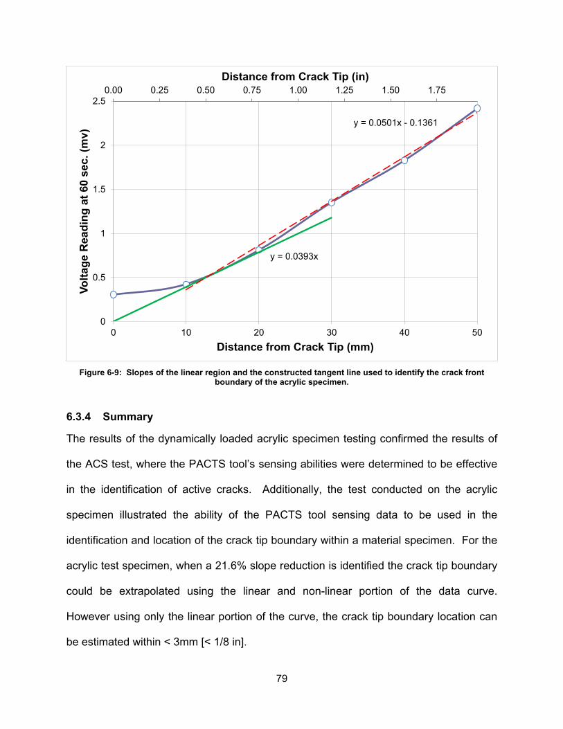
Figure 6-9: Slopes of the linear region and the constructed tangent line used to identify the crack front
boundary of the acrylic specimen.
6.3.4 Summary
The results of the dynamically loaded acrylic specimen testing confirmed the results of
the ACS test, where the PACTS tool’s sensing abilities were determined to be effective
in the identification of active cracks. Additionally, the test conducted on the acrylic
specimen illustrated the ability of the PACTS tool sensing data to be used in the
identification and location of the crack tip boundary within a material specimen. For the
acrylic test specimen, when a 21.6% slope reduction is identified the crack tip boundary
could be extrapolated using the linear and non-linear portion of the data curve.
However using only the linear portion of the curve, the crack tip boundary location can
be estimated within < 3mm [< 1/8 in].
y = 0.0393x
y = 0.0501x - 0.1361
0.00 0.25 0.50 0.75 1.00 1.25 1.50 1.75
0
0.5
1
1.5
2
2.5
0 10 20 30 40 50
Distance from Crack Tip (in) Vo
ltage
Rea
ding
at 6
0 se
c. (m
v)
Distance from Crack Tip (mm)
79

CHAPTER 7: SUMMARY AND CONCLUSION 7.1 Summary of Findings
The results of this research study successfully demonstrate the sensing ability of the
Piezoelectric Active Crack Tip Sensor (PACTS) tool in identifying active cracks and the
location of the crack tip boundary within a material. The results show a clear
relationship between the voltage sensing of the PACTS tool and the opening
displacement of a cracked surface at distances behind the crack tip boundary of a
dynamically loaded material. Active cracks with 0.056 mm [0.0022 in] opening
displacements were detected using an artificial crack system. Using a COLT analysis
technique, the new tool could be used immediately to determine planar crack tips to
within 3mm [0.12 in] accuracy without the use of a correction or modification factor on a
standard 38.1 mm [1.50 in] thick acrylic crack specimen. It was determined that if a
21.6% reduction in sensor slope with spatial length is detected, then the resulting crack
tip location could be determined to within 0.254 mm or 1/100th of an inch. Based on the
data, it was determined that the crack tip boundary location can be accurately identified
and documented in a material for future inspection, monitoring, or maintenance.
7.2 Conclusion
The sensitivity of the PACTS tool can effectively be used in the inspection and
monitoring of crack growth within bridges and other structures under dynamic loads.
The PACTS tool can be used to physically sweep across an active crack and identify
the location of the crack tip. Typically multiple cracks appear in a given structure
including those that branch off from an existing crack as shown in Figure 7-1, resulting
in multiple crack tips. However, the sensitivity of the PACTS system can potentially be
80
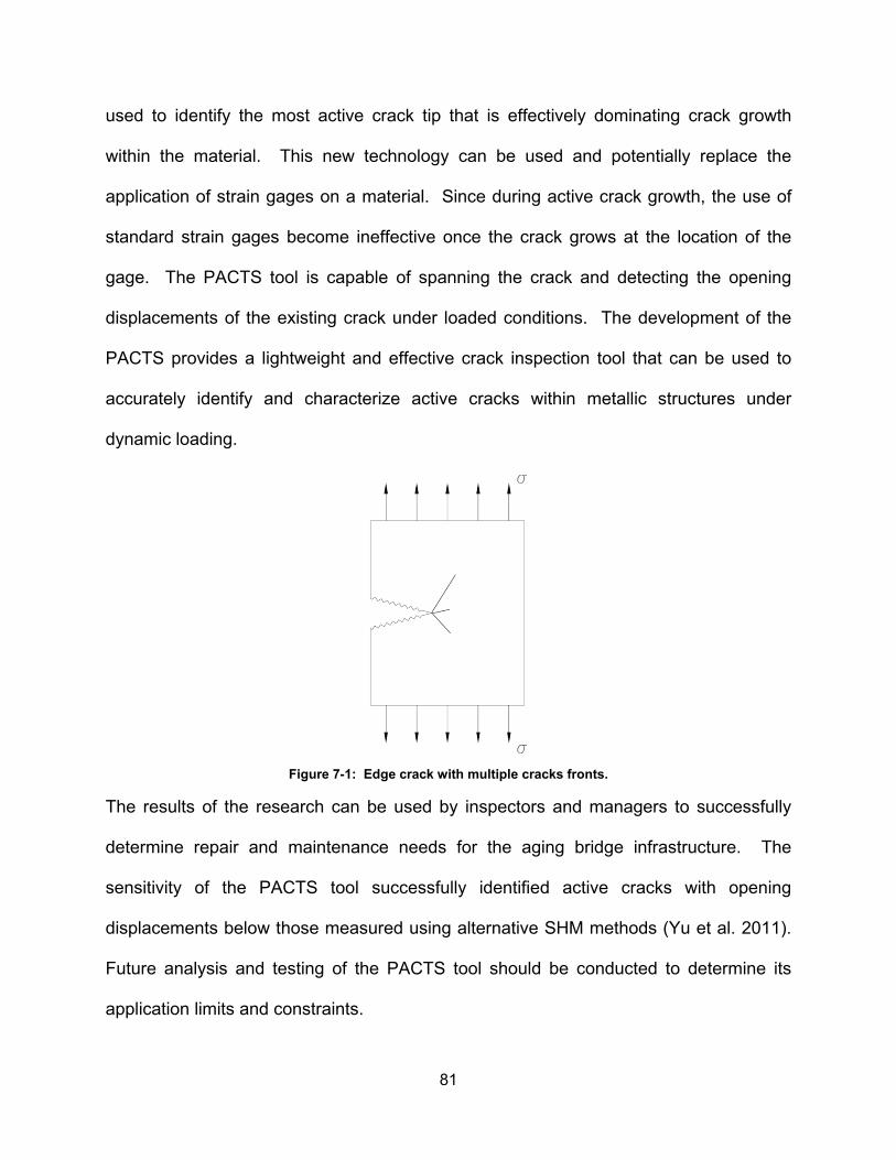
used to identify the most active crack tip that is effectively dominating crack growth
within the material. This new technology can be used and potentially replace the
application of strain gages on a material. Since during active crack growth, the use of
standard strain gages become ineffective once the crack grows at the location of the
gage. The PACTS tool is capable of spanning the crack and detecting the opening
displacements of the existing crack under loaded conditions. The development of the
PACTS provides a lightweight and effective crack inspection tool that can be used to
accurately identify and characterize active cracks within metallic structures under
dynamic loading.
Figure 7-1: Edge crack with multiple cracks fronts.
The results of the research can be used by inspectors and managers to successfully
determine repair and maintenance needs for the aging bridge infrastructure. The
sensitivity of the PACTS tool successfully identified active cracks with opening
displacements below those measured using alternative SHM methods (Yu et al. 2011).
Future analysis and testing of the PACTS tool should be conducted to determine its
application limits and constraints.
81

7.3 Recommendations for Future Work
The findings outlined in this dissertation demonstrate the potential for the PZT sensing
PACTS tool in the field of crack detection and characterizations. However, additional
investigations into the applications and sensitivity adjustments should be conducted
prior to marketing this sensor technology. Additional investigation can include but are
not limited to the following:
• Statistical analysis to determine which geometric parameter provides the
maximum effect on the effectiveness of the PACTS tool.
• Identification of opening displacement limitations on the PACTS tool.
• Using the crack tip identification technique on 3-dimensional cracked structures
with complex structural geometries and crack paths.
• Experimental testing of machine flawed specimens to determine ability to detect
subsurface discontinuities in a material.
• A comparison of crack detection ability with various other inspection techniques
and SHM systems.
• Experimental testing of pre-cracked steel structures under dynamic loading
including correlations between crack opening displacements and the sensing
capabilities of the PACTS system.
• Experimental testing on fatigue cracks in steel structures under dynamic loading.
• Field testing of in-service bridge structures with existing cracks.
82

REFERENCES
AASHTO (2008). Manual for Bridge Evaluation, American Association of State Highway and
Transportation Officials (AASHTO), Washington, DC.
Agarwal, B. D., and Bhagwan, D. A. (2006). Analysis and Performance of Fiber Composites,
Hoboken, N.J. : John Wiley, Hoboken, N.J.
ASCE (2013). "2013 Report Card for America's Infrastructure."
ASME (2010). "Rules for In Service Inspection for Nuclear Power Plant Components." ASME
Boiler and Pressure Vessel Code, ASME, New York.
ASTM (2012). "ASTM Standard E399-12e3." Standard Test Method for Linear-Elastic Plan-
Strain Fracture Toughness, KIC of Metallic Materials, ASTM International, West
Conshohocken, PA.
Barrett, R. M. (2013). "Introduction to Adaptive Aerostructures." University of Kansas.
Barsom, J. M., and Rolfe, S. T. (1999). Fracture and Fatigue Control in Structures : Applications
of Fracture Mechanics, ASTM, West Conshohocken, PA.
Boresi, A. P., and Schmidt, R. J. (2003). Advanced Mechanics of Materials, John Wiley & Sons,
New York.
Chopra, I., and Sirohi, J. (2013). Smart Structures Theory, Cambridge, England : Cambridge
University Press.
CTS (2013). "PZT5A AND 5H Product Data Sheets." <http://www.ctscorp.com/>. (7/7/2014,
2014).
FHWA (2001). "Reliability of Visual Inspection for Highway Bridges, Volume I: Final Report." F.
H. Administration, ed.McLean, VA.
FHWA (2011). "FHWA Brige Programs Structure Type by Year Built."
<www.fhwa.dot.gov/bridge/structyr.cfm>.
FHWA (2012). "Feasibility of Nondestructive Crack Detection and Monitoring for Steel Bridges."
F. H. Administration, ed.
Fuchs, H. O., and Stephens, R. I. (1980). Metal Fatigue in Engineering, Wiley, New York.
Gautschi, G. (2002). Piezoelectric Sensorics: Force, Strain, Pressure, Acceleration and Acoustic
Emission Sensors, Materials and Amplifiers, Springer - Verlag Berlin Heidelberg, Berlin.
Hellier, C. (2013). Handbook of Nondestructive Evaluation, McGraw-Hill, New York.
HSE (2006). "Probability of Detection (PoD) Curves: Derivations, applications and limitations."
Health and Safety Executive, London.
83

Ihn, J. B., Chang, F. K., Ihn, J. B., and Chang, F. K. (2004). "Detection and Monitoring of Hidden
Fatigue Crack Growth Using a Built-In Piezoelectric Sensor/Actuator Network: I.
Diagnostics." Smart Mater. Struct., 13(3), 609-620.
Jalinoos, F. (2009). "NDE Showcase for Bridge Inspectors." FHWA, ed.
Jones, R. M. (1975). Mechanics of Composite Materials, Washington, Scripta Book Co.,
Washington.
Lynch, J. P. (2004). "Detection of Structural Cracks Using Piezoelectric Active Sensors." 17th
ASCE Engineering Mechanics Conference, ASCE, University of Delaware, Newark, DE.
Morgan Advanced Materials (2009). <http://www.morganelectroceramics.com/>. (6/10/2014,
2014).
NDEC, N. E. C. (2010). "NDEC News." FHWA, ed.
Piezo Systems Inc. (2011). <http://piezo.com/>. (4/12/2013, 2013).
Purvis, R. L. (1988). "Inspection of Fracture Critical Bridge Members." Transportation Research
Record(1184).
Rolfe, S. T. (1993). "Fitness for Service - Common Sense Enginering." Proc., The Art and
Science of Structural Engineering : proceedings of the symposium honoring William J.
Hall, Prentice Hall, xxxiii, 238 p.
Sanford, R. J. (2003). Principles of Fracture Mechanics, Prentice Hall, Upper Saddle River, NJ.
Silva, A. S. S., Oliveira, D. F., Machado, A. S., Nascimento, J. R., and Lopes, R. T. (2014). "An
Evaluation of Imaging Plate Characteristics that Determine Image Quality in Computed
Radiography." Mater Eval, American Society of Nondestructive Testing, Columbus,
Ohio.
Sirohi, J., and Chopra, I. (2000). "Fundamental understanding of piezoelectric strain sensors." J.
Intell. Mater. Syst. Struct., 11(4), 246-257.
Wells, A. A. (1981). "The Meaning of Fitness-for-Purpose and Concept of Defect Tolerance."
International Conference, The Welding Institute, London.
Whisler, D. (2013). "KU Research - Bridge Inspection Questions." A. M. Elmore, ed., Kansas
Department of Transportation (KDOT).
Yu, L., Momeni, S., Godinez, V., and Giurgiutiu, V. "Adaptation of PWAS Transducers to
Acoustic Emission Sensors." Proc., Nondestructive Characterization for Composite
Materials, Aerospace Engineering, Civil Infrastructure, and Homeland Security, SPIE.
Zhang, Y. F. (2006). "In Situ Fatigue Crack Detection Using Piezoelectric Paint Sensor." J Intel
Mat Syst Str, 17(10), 843-852.
84

APPENDIXES
85

APPENDIX A: MATERIAL PROPERTIES
A.1 Metric Units
86

A.2 English Units
87

APPENDIX B: GENERAL DESIGN AND MANUFACTURING PROCESS
B.1 General Design of Fabricated Aluminum Substrate H-Beam
88

B.2 Manufacturing Procedure Tools and Equipment
Piezoceramic Sheet of Desired Thickness
Aluminum Substrate (General H-frame geometry)
M4 x 0.7 (8-32) Steel Screws
Rotary Diamond Saw
Sand Paper (320-600 grit)
Conducting Epoxy (EP21TDC/N)
De-waxing and Cleaning Agents
Neodymium Magnet with 1 Countersunk Hole
Tix Solder
Soldering Iron
Variable Speed Lathe
Milling Machine Fabrication Procedures
1. Substrate Preparation
i. Mill the substrate H-beam web to the desired thickness.
Figure B-1: General H-beam geometry in milling machine.
89

ii. Clean aluminum substrate with propanol and wet-sand to remove oxide
layers.
2. Piezoelectric Element Preparation
i. Mark the element to extend beyond the required substrate width.
Figure B-2: Piezoceramic sheet
ii. Cut the element using the rotary diamond saw under wet conditions to
capture and remove potential dust and airborne lead hazards.
Figure B-3: Diamond saw used to cut the piezoceramic sheets.
90

iii. Wet sand the piezoceramic sheet using 320-600 grit sand paper to
remove sputtered nickel facing.
Figure B-4: Piezoceramic sheet and 340 grit sand paper.
iv. Clean the element and remove all debris from both surfaces.
v. Determine and mark the poling direction of the PZT.
3. Resin Preparation
i. Select the resin to be used or EP21TDC/N.
ii. Mix the resin in proper proportions according to the manufacturers
recommendations.
iii. Smear the mixed epoxy along the substrate web. Make sure the layer is
very thin.
91

4. Substrate Mounting
i. Mount the dry piezoceramic sheet to the epoxy coated side of the
substrate web. Gently work the excess resin to the edges of the web.
ii. Insert the unimorph into a vice, cover the piezoelectric mounted section,
and apply a small weight to the surface in order to hold bonded parts in
contact.
iii. Let cure in accordance to the epoxy instructions.
iv. Once cured, sand piezoelectric edge surfaces till smooth and flush with
substrate web width.
5. Leg assembly
i. Remove steel screw head and grind shaft tip using the variable speed
lathe to fit magnet countersunk dimensions.
(a)
(b)
Figure B-5: (a) Variable speed lathe used to remove the (b) steel screw head and sharpen the shaft tip.
92

ii. Clean the steel screw and mount to magnet using Hysol 9412.
Figure B-6: Cleaned steel screw mounted to countersunk magnet.
iii. Let cure in accordance to manufacturers recommendations.
Figure B-7: PACTS tool leg assembly with sharpened steel screw and countersunk magnet.
6. PACTS tool assembly
i. Anchor one lead mechanically and electrically to the ground of the H-
frame.
ii. Solder the second lead to the top of the piezoceramic sensor sheet using
Tix solder.
93

Figure B-8: Two PACTS tool composite members with leads grounded to the substrate frame and soldered
to top of the piezoceramic sensor sheet.
iii. Route the two leads to the RC charge-sensor circuit and voltmeter.
7. PACTS tool Assembly
i. Insert steel legs into drilled and tapped substrate flange holes.
Figure B-9: Fabricated PACTS tools.
94

APPENDIX C: ABAQUS OPTIMIZATION
C.1 Results of Bond Thickness Variation on the PACTS Sensing Ability
Figure C-1: FE model results of PACTS voltage sensitivity for a 0.254 mm [0.010 in] PZT layer thickness as a function of the aluminum thickness and bond thicknesses ranging from 0.0254 mm [0.001 in] ≤ tb ≥ 6.350 mm
[0.250 in].
Figure C-2: FE model results of PACTS voltage sensitivity for a 0.508 mm [0.020 in] PZT layer thickness as a function of the aluminum thickness and bond thicknesses ranging from 0.0254 mm [0.001 in] ≤ tb ≥ 6.35 mm
[0.250 in].
95

Figure C-3: FE model results of PACTS voltage sensitivity for a 1.016 mm [0.040 in] PZT layer thickness as a function of the aluminum thickness and bond thicknesses ranging from 0.0254 mm [0.001 in] ≤ tb ≥ 6.35 mm
[0.250 in].
Figure C-4: FE model results of PACTS voltage sensitivity for a 2.032 mm [0.080 in] PZT layer thickness as a function of the aluminum thickness and bond thicknesses ranging from 0.0254 mm [0.001 in] ≤ tb ≥ 6.35 mm
[0.250 in].
96

Figure C-5: FE model results of PACTS voltage sensitivity for a 2.540 mm [0.100 in] PZT layer thickness as a function of the aluminum thickness and bond thicknesses ranging from 0.0254 mm [0.001 in] ≤ tb ≥ 6.35 mm
[0.250 in].
C.2 Results of PZT Thickness Variation on the PACTS Sensing Ability
Figure C-6: FE model results of PACTS voltage sensitivity as a function of PZT layer thicknesses and
aluminum substrate thickness using a constant 0.0254 mm [0.001 in] bond layer thickness.
97
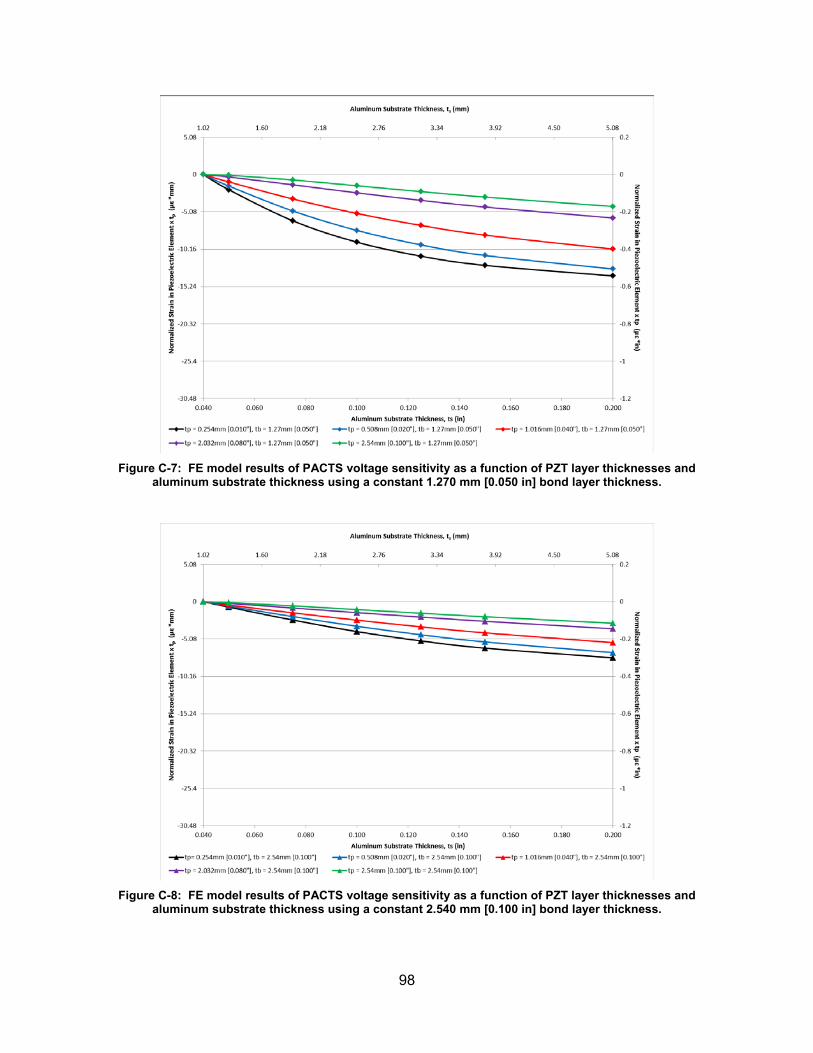
Figure C-7: FE model results of PACTS voltage sensitivity as a function of PZT layer thicknesses and
aluminum substrate thickness using a constant 1.270 mm [0.050 in] bond layer thickness.
Figure C-8: FE model results of PACTS voltage sensitivity as a function of PZT layer thicknesses and
aluminum substrate thickness using a constant 2.540 mm [0.100 in] bond layer thickness.
98

Figure C-9: FE model results of PACTS voltage sensitivity as a function of PZT layer thicknesses and
aluminum substrate thickness using a constant 5.080 mm [0.200 in] bond layer thickness.
Figure C-10: FE model results of PACTS voltage sensitivity as a function of PZT layer thicknesses and
aluminum substrate thickness using a constant 6.350 mm [0.250 in] bond layer thickness.
99

C.3 Finite Element Model Data and Calculated Sensing Voltage Table C-1: FE model PACTS tool PZT layer mid-plane strain results and voltage sensitivity calculations as a
function of substrate and bond thicknesses using a constant 0.254 mm [0.010 in] PZT layer thickness.
Model ts tb με ɛ x tp in mm in mm normalized με*in με*mm
ts40_tb1_tp10 0.040 1.016 0.001 0.0254 0.0 0 0 ts50_tb1_tp10 0.050 1.270 0.001 0.0254 -28.5 -0.285 -7.239 ts75_tb1_tp10 0.075 1.905 0.001 0.0254 -63.5 -0.635 -16.132 ts100_tb1_tp10 0.100 2.540 0.001 0.0254 -78.4 -0.784 -19.905 ts125_tb1_tp10 0.125 3.175 0.001 0.0254 -86.0 -0.860 -21.835 ts150_tb1_tp10 0.150 3.810 0.001 0.0254 -90.3 -0.903 -22.948 ts200_tb1_tp10 0.200 5.080 0.001 0.0254 -94.9 -0.949 -24.112 ts40_tb50_tp10 0.040 1.016 0.05 1.27 0.0 0 0 ts50_tb50_tp10 0.050 1.270 0.05 1.27 -8.1 -0.081 -2.063 ts75_tb50_tp10 0.075 1.905 0.05 1.27 -24.8 -0.248 -6.296 ts100_tb50_tp10 0.100 2.540 0.05 1.27 -36.2 -0.362 -9.200 ts125_tb50_tp10 0.125 3.175 0.05 1.27 -43.7 -0.437 -11.106 ts150_tb50_tp10 0.150 3.810 0.05 1.27 -48.7 -0.487 -12.361 ts200_tb50_tp10 0.200 5.080 0.050 1.27 -54.3 -0.543 -13.791 ts40_tb100_tp10 0.040 1.016 0.100 2.54 0.0 0 0 ts50_tb100_tp10 0.050 1.270 0.100 2.54 -2.9 -0.029 -0.732 ts75_tb100_tp10 0.075 1.905 0.100 2.54 -9.8 -0.098 -2.501 ts100_tb100_tp10 0.100 2.540 0.100 2.54 -16.0 -0.160 -4.067 ts125_tb100_tp10 0.125 3.175 0.100 2.54 -21.0 -0.210 -5.342 ts150_tb100_tp10 0.150 3.810 0.100 2.54 -24.9 -0.249 -6.328 ts200_tb100_tp10 0.200 5.080 0.100 2.54 -30.1 -0.301 -7.636 ts40_tb200_tp10 0.040 1.016 0.200 5.08 0.0 0 0 ts50_tb200_tp10 0.050 1.270 0.200 5.08 -0.9 -0.009 -0.222 ts75_tb200_tp10 0.075 1.905 0.200 5.08 -3.0 -0.030 -0.761 ts100_tb200_tp10 0.100 2.540 0.200 5.08 -5.1 -0.051 -1.301 ts125_tb200_tp10 0.125 3.175 0.200 5.08 -7.2 -0.072 -1.826 ts150_tb200_tp10 0.150 3.810 0.200 5.08 -9.1 -0.091 -2.315 ts200_tb200_tp10 0.200 5.080 0.200 5.08 -12.3 -0.123 -3.132 ts40_tb250_tp10 0.040 1.016 0.250 6.35 0.0 0 0 ts50_tb250_tp10 0.050 1.270 0.250 6.35 -0.6 -0.006 -0.155 ts75_tb250_tp10 0.075 1.905 0.250 6.35 -2.0 -0.020 -0.516 ts100_tb250_tp10 0.100 2.540 0.250 6.35 -3.4 -0.034 -0.874 ts125_tb250_tp10 0.125 3.175 0.250 6.35 -4.8 -0.048 -1.232 ts150_tb250_tp10 0.150 3.810 0.250 6.35 -6.2 -0.062 -1.579 ts200_tb250_tp10 0.200 5.080 0.250 6.35 -8.7 -0.087 -2.204
100
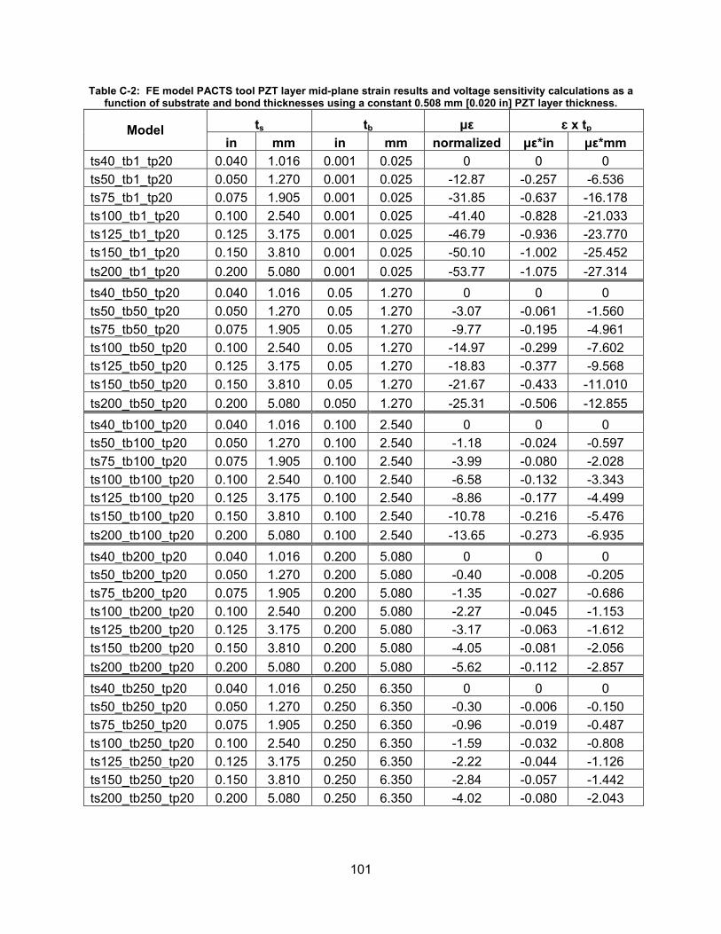
Table C-2: FE model PACTS tool PZT layer mid-plane strain results and voltage sensitivity calculations as a function of substrate and bond thicknesses using a constant 0.508 mm [0.020 in] PZT layer thickness.
Model ts tb με ɛ x tp in mm in mm normalized με*in με*mm
ts40_tb1_tp20 0.040 1.016 0.001 0.025 0 0 0 ts50_tb1_tp20 0.050 1.270 0.001 0.025 -12.87 -0.257 -6.536 ts75_tb1_tp20 0.075 1.905 0.001 0.025 -31.85 -0.637 -16.178 ts100_tb1_tp20 0.100 2.540 0.001 0.025 -41.40 -0.828 -21.033 ts125_tb1_tp20 0.125 3.175 0.001 0.025 -46.79 -0.936 -23.770 ts150_tb1_tp20 0.150 3.810 0.001 0.025 -50.10 -1.002 -25.452 ts200_tb1_tp20 0.200 5.080 0.001 0.025 -53.77 -1.075 -27.314 ts40_tb50_tp20 0.040 1.016 0.05 1.270 0 0 0 ts50_tb50_tp20 0.050 1.270 0.05 1.270 -3.07 -0.061 -1.560 ts75_tb50_tp20 0.075 1.905 0.05 1.270 -9.77 -0.195 -4.961 ts100_tb50_tp20 0.100 2.540 0.05 1.270 -14.97 -0.299 -7.602 ts125_tb50_tp20 0.125 3.175 0.05 1.270 -18.83 -0.377 -9.568 ts150_tb50_tp20 0.150 3.810 0.05 1.270 -21.67 -0.433 -11.010 ts200_tb50_tp20 0.200 5.080 0.050 1.270 -25.31 -0.506 -12.855 ts40_tb100_tp20 0.040 1.016 0.100 2.540 0 0 0 ts50_tb100_tp20 0.050 1.270 0.100 2.540 -1.18 -0.024 -0.597 ts75_tb100_tp20 0.075 1.905 0.100 2.540 -3.99 -0.080 -2.028 ts100_tb100_tp20 0.100 2.540 0.100 2.540 -6.58 -0.132 -3.343 ts125_tb100_tp20 0.125 3.175 0.100 2.540 -8.86 -0.177 -4.499 ts150_tb100_tp20 0.150 3.810 0.100 2.540 -10.78 -0.216 -5.476 ts200_tb100_tp20 0.200 5.080 0.100 2.540 -13.65 -0.273 -6.935 ts40_tb200_tp20 0.040 1.016 0.200 5.080 0 0 0 ts50_tb200_tp20 0.050 1.270 0.200 5.080 -0.40 -0.008 -0.205 ts75_tb200_tp20 0.075 1.905 0.200 5.080 -1.35 -0.027 -0.686 ts100_tb200_tp20 0.100 2.540 0.200 5.080 -2.27 -0.045 -1.153 ts125_tb200_tp20 0.125 3.175 0.200 5.080 -3.17 -0.063 -1.612 ts150_tb200_tp20 0.150 3.810 0.200 5.080 -4.05 -0.081 -2.056 ts200_tb200_tp20 0.200 5.080 0.200 5.080 -5.62 -0.112 -2.857 ts40_tb250_tp20 0.040 1.016 0.250 6.350 0 0 0 ts50_tb250_tp20 0.050 1.270 0.250 6.350 -0.30 -0.006 -0.150 ts75_tb250_tp20 0.075 1.905 0.250 6.350 -0.96 -0.019 -0.487 ts100_tb250_tp20 0.100 2.540 0.250 6.350 -1.59 -0.032 -0.808 ts125_tb250_tp20 0.125 3.175 0.250 6.350 -2.22 -0.044 -1.126 ts150_tb250_tp20 0.150 3.810 0.250 6.350 -2.84 -0.057 -1.442 ts200_tb250_tp20 0.200 5.080 0.250 6.350 -4.02 -0.080 -2.043
101

Table C-3: FE model PACTS tool PZT layer mid-plane strain results and voltage sensitivity calculations as a function of substrate and bond thicknesses using a constant 1.016 mm [0.040 in] PZT layer thickness.
Model ts tb με ɛ x tp in mm in mm normalized με*in με*mm
ts40_tb1_tp40 0.040 1.016 0.001 0.0254 0 0 0 ts50_tb1_tp40 0.050 1.270 0.001 0.0254 -3.2 -0.128 -3.261 ts75_tb1_tp40 0.075 1.905 0.001 0.0254 -9.6 -0.386 -9.792 ts100_tb1_tp40 0.100 2.540 0.001 0.0254 -13.9 -0.556 -14.122 ts125_tb1_tp40 0.125 3.175 0.001 0.0254 -16.7 -0.669 -16.999 ts150_tb1_tp40 0.150 3.810 0.001 0.0254 -18.7 -0.747 -18.971 ts200_tb1_tp40 0.200 5.080 0.001 0.0254 -21.1 -0.842 -21.393 ts40_tb50_tp40 0.040 1.016 0.05 1.27 0 0 0 ts50_tb50_tp40 0.050 1.270 0.05 1.27 -1.0 -0.039 -1.002 ts75_tb50_tp40 0.075 1.905 0.05 1.27 -3.3 -0.131 -3.320 ts100_tb50_tp40 0.100 2.540 0.05 1.27 -5.2 -0.208 -5.295 ts125_tb50_tp40 0.125 3.175 0.05 1.27 -6.8 -0.273 -6.922 ts150_tb50_tp40 0.150 3.810 0.05 1.27 -8.1 -0.324 -8.237 ts200_tb50_tp40 0.200 5.080 0.050 1.27 -10.0 -0.399 -10.142 ts40_tb100_tp40 0.040 1.016 0.100 2.54 0 0 0 ts50_tb100_tp40 0.050 1.270 0.100 2.54 -0.4 -0.018 -0.449 ts75_tb100_tp40 0.075 1.905 0.100 2.54 -1.5 -0.060 -1.518 ts100_tb100_tp40 0.100 2.540 0.100 2.54 -2.5 -0.099 -2.514 ts125_tb100_tp40 0.125 3.175 0.100 2.54 -3.4 -0.135 -3.424 ts150_tb100_tp40 0.150 3.810 0.100 2.54 -4.2 -0.167 -4.239 ts200_tb100_tp40 0.200 5.080 0.100 2.54 -5.5 -0.220 -5.580 ts40_tb200_tp40 0.040 1.016 0.200 5.08 0 0 0 ts50_tb200_tp40 0.050 1.270 0.200 5.08 -0.2 -0.007 -0.180 ts75_tb200_tp40 0.075 1.905 0.200 5.08 -0.6 -0.023 -0.589 ts100_tb200_tp40 0.100 2.540 0.200 5.08 -1.0 -0.038 -0.973 ts125_tb200_tp40 0.125 3.175 0.200 5.08 -1.3 -0.053 -1.346 ts150_tb200_tp40 0.150 3.810 0.200 5.08 -1.7 -0.067 -1.709 ts200_tb200_tp40 0.200 5.080 0.200 5.08 -2.4 -0.094 -2.396 ts40_tb250_tp40 0.040 1.016 0.250 6.35 0 0 0 ts50_tb250_tp40 0.050 1.270 0.250 6.35 -0.1 -0.005 -0.138 ts75_tb250_tp40 0.075 1.905 0.250 6.35 -0.4 -0.017 -0.438 ts100_tb250_tp40 0.100 2.540 0.250 6.35 -0.7 -0.028 -0.712 ts125_tb250_tp40 0.125 3.175 0.250 6.35 -1.0 -0.038 -0.978 ts150_tb250_tp40 0.150 3.810 0.250 6.35 -1.2 -0.049 -1.240 ts200_tb250_tp40 0.200 5.080 0.250 6.35 -1.7 -0.069 -1.755
102

Table C-4: FE model PACTS tool PZT layer mid-plane strain results and voltage sensitivity calculations as a function of substrate and bond thicknesses using a constant 2.032 mm [0.080 in] PZT layer thickness.
Model ts tb με ɛ x tp in mm in mm normalized με*in με*mm
ts40_tb1_tp80 0.040 1.016 0.001 0.025 0 0 0 ts50_tb1_tp80 0.050 1.270 0.001 0.025 -0.134 -0.011 -0.271 ts75_tb1_tp80 0.075 1.905 0.001 0.025 -1.025 -0.082 -2.082 ts100_tb1_tp80 0.100 2.540 0.001 0.025 -2.038 -0.163 -4.142 ts125_tb1_tp80 0.125 3.175 0.001 0.025 -2.928 -0.234 -5.950 ts150_tb1_tp80 0.150 3.810 0.001 0.025 -3.661 -0.293 -7.439 ts200_tb1_tp80 0.200 5.080 0.001 0.025 -4.733 -0.379 -9.618 ts40_tb50_tp80 0.040 1.016 0.05 1.270 0 0 0 ts50_tb50_tp80 0.050 1.270 0.05 1.270 -0.163 -0.013 -0.332 ts75_tb50_tp80 0.075 1.905 0.05 1.270 -0.684 -0.055 -1.390 ts100_tb50_tp80 0.100 2.540 0.05 1.270 -1.224 -0.098 -2.488 ts125_tb50_tp80 0.125 3.175 0.05 1.270 -1.726 -0.138 -3.508 ts150_tb50_tp80 0.150 3.810 0.05 1.270 -2.175 -0.174 -4.419 ts200_tb50_tp80 0.200 5.080 0.050 1.270 -2.911 -0.233 -5.915 ts40_tb100_tp80 0.040 1.016 0.100 2.540 0 0 0 ts50_tb100_tp80 0.050 1.270 0.100 2.540 -0.112 -0.009 -0.227 ts75_tb100_tp80 0.075 1.905 0.100 2.540 -0.420 -0.034 -0.853 ts100_tb100_tp80 0.100 2.540 0.100 2.540 -0.732 -0.059 -1.487 ts125_tb100_tp80 0.125 3.175 0.100 2.540 -1.031 -0.083 -2.096 ts150_tb100_tp80 0.150 3.810 0.100 2.540 -1.313 -0.105 -2.668 ts200_tb100_tp80 0.200 5.080 0.100 2.540 -1.813 -0.145 -3.684 ts40_tb200_tp80 0.040 1.016 0.200 5.080 0 0 0 ts50_tb200_tp80 0.050 1.270 0.200 5.080 -0.064 -0.005 -0.130 ts75_tb200_tp80 0.075 1.905 0.200 5.080 -0.214 -0.017 -0.434 ts100_tb200_tp80 0.100 2.540 0.200 5.080 -0.356 -0.028 -0.724 ts125_tb200_tp80 0.125 3.175 0.200 5.080 -0.494 -0.040 -1.004 ts150_tb200_tp80 0.150 3.810 0.200 5.080 -0.628 -0.050 -1.276 ts200_tb200_tp80 0.200 5.080 0.200 5.080 -0.888 -0.071 -1.805 ts40_tb250_tp80 0.040 1.016 0.250 6.350 0 0 0 ts50_tb250_tp80 0.050 1.270 0.250 6.350 -0.054 -0.004 -0.109 ts75_tb250_tp80 0.075 1.905 0.250 6.350 -0.172 -0.014 -0.349 ts100_tb250_tp80 0.100 2.540 0.250 6.350 -0.279 -0.022 -0.567 ts125_tb250_tp80 0.125 3.175 0.250 6.350 -0.381 -0.031 -0.775 ts150_tb250_tp80 0.150 3.810 0.250 6.350 -0.481 -0.038 -0.977 ts200_tb250_tp80 0.200 5.080 0.250 6.350 -0.680 -0.054 -1.381
103

Table C-5: FE model PACTS tool PZT layer mid-plane strain results and voltage sensitivity calculations as a function of substrate and bond thicknesses using a constant 2.540 mm [0.100 in] PZT layer thickness.
Model ts tb με ɛ x tp in mm in mm normalized με*in με*mm
ts40_tb1_tp100 0.040 1.016 0.001 0.025 0 0 0 ts50_tb1_tp100 0.050 1.270 0.001 0.025 0.095 0.010 0.242 ts75_tb1_tp100 0.075 1.905 0.001 0.025 -0.170 -0.017 -0.432 ts100_tb1_tp100 0.100 2.540 0.001 0.025 -0.674 -0.067 -1.711 ts125_tb1_tp100 0.125 3.175 0.001 0.025 -1.190 -0.119 -3.022 ts150_tb1_tp100 0.150 3.810 0.001 0.025 -1.654 -0.165 -4.201 ts200_tb1_tp100 0.200 5.080 0.001 0.025 -2.392 -0.239 -6.075 ts40_tb50_tp100 0.040 1.016 0.05 1.270 0 0 0 ts50_tb50_tp100 0.050 1.270 0.05 1.270 -0.040 -0.004 -0.102 ts75_tb50_tp100 0.075 1.905 0.05 1.270 -0.288 -0.029 -0.731 ts100_tb50_tp100 0.100 2.540 0.05 1.270 -0.600 -0.060 -1.523 ts125_tb50_tp100 0.125 3.175 0.05 1.270 -0.912 -0.091 -2.317 ts150_tb50_tp100 0.150 3.810 0.05 1.270 -1.205 -0.121 -3.061 ts200_tb50_tp100 0.200 5.080 0.050 1.270 -1.710 -0.171 -4.342 ts40_tb100_tp100 0.040 1.016 0.100 2.540 0 0 0 ts50_tb100_tp100 0.050 1.270 0.100 2.540 -0.050 -0.005 -0.126 ts75_tb100_tp100 0.075 1.905 0.100 2.540 -0.224 -0.022 -0.569 ts100_tb100_tp100 0.100 2.540 0.100 2.540 -0.420 -0.042 -1.068 ts125_tb100_tp100 0.125 3.175 0.100 2.540 -0.617 -0.062 -1.568 ts150_tb100_tp100 0.150 3.810 0.100 2.540 -0.807 -0.081 -2.050 ts200_tb100_tp100 0.200 5.080 0.100 2.540 -1.154 -0.115 -2.932 ts40_tb200_tp100 0.040 1.016 0.200 5.080 0 0 0 ts50_tb200_tp100 0.050 1.270 0.200 5.080 -0.039 -0.004 -0.100 ts75_tb200_tp100 0.075 1.905 0.200 5.080 -0.139 -0.014 -0.352 ts100_tb200_tp100 0.100 2.540 0.200 5.080 -0.237 -0.024 -0.603 ts125_tb200_tp100 0.125 3.175 0.200 5.080 -0.334 -0.033 -0.848 ts150_tb200_tp100 0.150 3.810 0.200 5.080 -0.428 -0.043 -1.088 ts200_tb200_tp100 0.200 5.080 0.200 5.080 -0.614 -0.061 -1.559 ts40_tb250_tp100 0.040 1.016 0.250 6.350 0 0 0 ts50_tb250_tp100 0.050 1.270 0.250 6.350 -0.026 -0.003 -0.066 ts75_tb250_tp100 0.075 1.905 0.250 6.350 -0.117 -0.012 -0.298 ts100_tb250_tp100 0.100 2.540 0.250 6.350 -0.194 -0.019 -0.492 ts125_tb250_tp100 0.125 3.175 0.250 6.350 -0.267 -0.027 -0.677 ts150_tb250_tp100 0.150 3.810 0.250 6.350 -0.338 -0.034 -0.858 ts200_tb250_tp100 0.200 5.080 0.250 6.350 -0.481 -0.048 -1.221
104

C.4 Selected Geometry
105
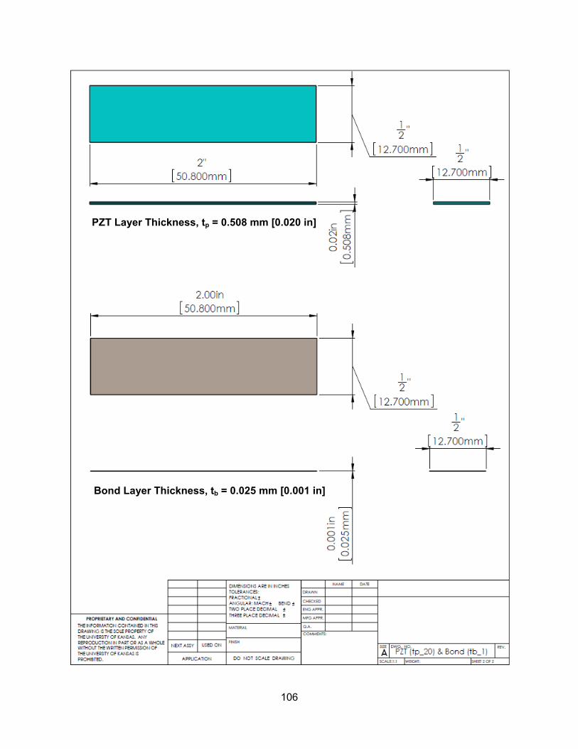
PZT Layer Thickness, tp = 0.508 mm [0.020 in]
Bond Layer Thickness, tb = 0.025 mm [0.001 in]
106

107
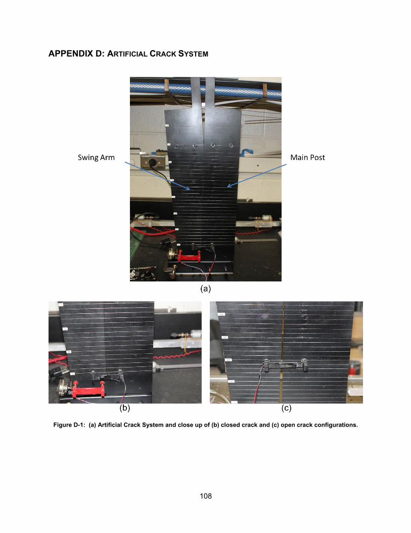
APPENDIX D: ARTIFICIAL CRACK SYSTEM
Figure D-1: (a) Artificial Crack System and close up of (b) closed crack and (c) open crack configurations.
108

D.1 Artificial Crack System Geometry
Figure D-2: Drawing of Artificial Crack System Main Post
109
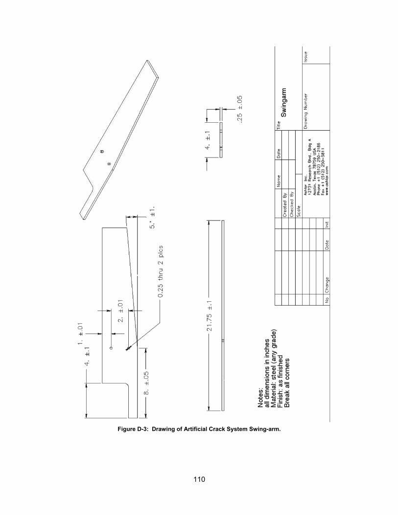
Figure D-3: Drawing of Artificial Crack System Swing-arm.
110
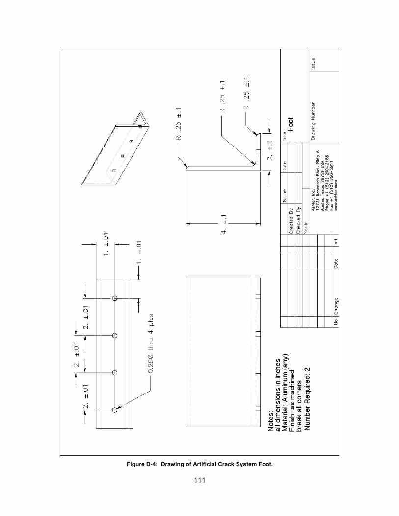
Figure D-4: Drawing of Artificial Crack System Foot.
111

Figure D-5: Drawing of Artificial Crack System Hinge Piece 1.
112

Figure D-6: Drawing of Artificial Crack System Hinge Piece 2.
113

D.2 Artificial Crack System Experimental Data Table D-1: Artificial Crack System experimental results
Distance from Crack Center
Reading at 60 seconds
mm in mV 0 0 2 10 0.394 1 20 0.787 1 30 1.18 1 40 1.57 2 50 1.97 2
100 3.94 4 150 5.91 6 200 7.87 8 250 9.84 10 300 11.8 12
114

APPENDIX E: ACRYLIC SPECIMEN TEST DOCUMENTS
E.1 ASTM E399 Geometry
115

116
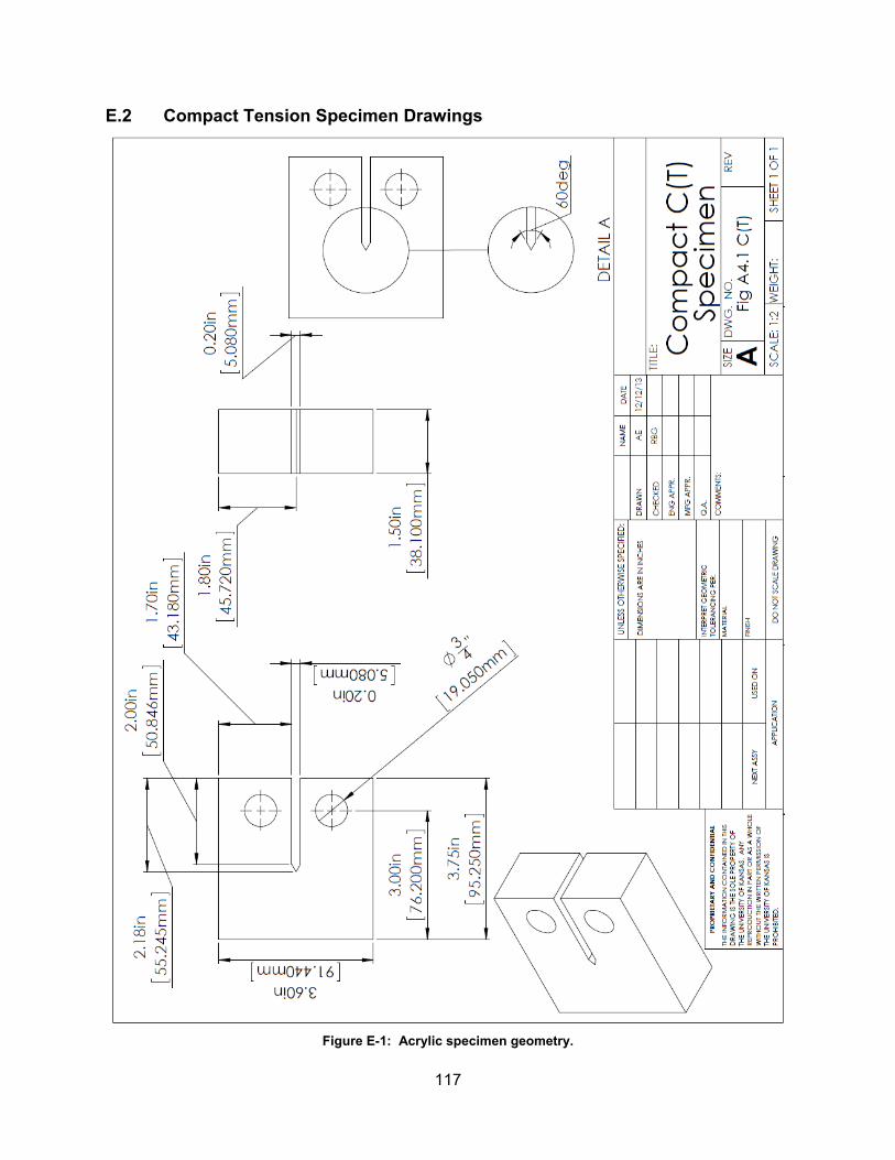
E.2 Compact Tension Specimen Drawings
Figure E-1: Acrylic specimen geometry.
117

E.3 Acrylic Specimen Dynamic Test Results Table E-1: Experimental results for acrylic proof of concept testing.
Distance from Crack Tip
Voltage Reading at 60 sec.
mm in (mV) 50 1.969 0 40 1.575 2.42 30 1.181 1.83 20 0.787 1.35 10 0.394 0.813 0 0 0.423
-10 -0.394 0.308 -20 -0.787 0.226
Figure E-2: Acrylic specimen test voltage reading results at distances ahead and behind the crack tip
boundary with linear trend lines.
118

Figure E-3: Acrylic specimen test voltage reading results at distances behind the crack tip and the
approximated crack tip boundary location using the using the extension on the linear portion of the results and zero voltage.
Figure E-4: Acrylic specimen test voltage reading results at distances behind the crack tip and the equation
of the non-linear section used in the crack tip location analysis.
y = 0.0501x - 0.1361
-0.79 -0.29 0.21 0.71 1.21 1.71
-0.5
0
0.5
1
1.5
2
2.5
0 10 20 30 40 50
Distance from Crack Center (in)
Volta
ge R
eadi
ng a
t 60
sec.
(mV)
Distance from Crack Center (mm)
Distance = 2.72 mm [0.11 in]
y = 0.0014x2 - 0.0022x + 0.308
-0.79 -0.29 0.21 0.71 1.21 1.71
0
0.5
1
1.5
2
2.5
-20 -10 0 10 20 30 40 50
Distance from Crack Tip (in)
Volta
ge R
eadi
ng a
t 60
sec.
(mV)
Distance from Crack Tip (mm)
119

Figure E-5: Acrylic specimen test voltage reading results at distances behind the crack tip and the equations of the non-linear section used in the crack tip location analysis and the line tangent to the non-linear region
through the crack tip boundary.
y = 0.0014x2 - 0.0022x + 0.308
0.00 0.50 1.00 1.50
0
0.5
1
1.5
2
2.5
0 10 20 30 40 50
Distance from Crack Center (in) Vo
ltage
Rea
ding
at 6
0 se
c. (m
V)
Distance from Crack Center (mm)
y = 0.03933x
(14.832, 0.583)
120

E.4 Calculation of Crack Tip Boundary Location
121

E.5 Acrylic Compact Tension Specimen Ultimate Load
Figure E-6: Ultimate load of 1704 N [383 lb] determined experimentally for the acrylic specimen material used
in the PACTS tool proof of concept testing.
0
50
100
150
200
250
300
350
400
0 0.005 0.01 0.015 0.02 0.025 0.03 0.035
0
200
400
600
800
1000
1200
1400
1600
1800
0 0.1 0.2 0.3 0.4 0.5 0.6 0.7 0.8 0.9
Applied Load (lb)
Vertical Displacement (in)
Appl
ied
Load
(N)
Vertical Displacement (mm)
Ultimate Load = 1704 N [383 lb]
122

Table E-2: Acrylic compact tension specimen ultimate load test data.
Vertical Position Load
Vertical Position Load
mm in N lb mm in N lb 1 0 0 204.608 46 41 0.13716 0.0054 418.112 94 2 0.00508 0.0002 213.504 48 42 0.14478 0.0057 422.56 95 3 0.00508 0.0002 217.952 49 43 0.14478 0.0057 427.008 96 4 0.0127 0.0005 226.848 51 44 0.14986 0.0059 431.456 97 5 0.0127 0.0005 235.744 53 45 0.14986 0.0059 435.904 98 6 0.01778 0.0007 244.64 55 46 0.14986 0.0059 435.904 98 7 0.01778 0.0007 249.088 56 47 0.15748 0.0062 440.352 99 8 0.02286 0.0009 257.984 58 48 0.15748 0.0062 444.8 100 9 0.03048 0.0012 262.432 59 49 0.15748 0.0062 449.248 101 10 0.03048 0.0012 266.88 60 50 0.1651 0.0065 453.696 102 11 0.03556 0.0014 275.776 62 51 0.1651 0.0065 453.696 102 12 0.03556 0.0014 280.224 63 52 0.1651 0.0065 458.144 103 13 0.04318 0.0017 284.672 64 53 0.17018 0.0067 462.592 104 14 0.04826 0.0019 289.12 65 54 0.17018 0.0067 467.04 105 15 0.04826 0.0019 298.016 67 55 0.1778 0.007 467.04 105 16 0.05588 0.0022 302.464 68 56 0.1778 0.007 471.488 106 17 0.0635 0.0025 306.912 69 57 0.1778 0.007 475.936 107 18 0.0635 0.0025 311.36 70 58 0.18288 0.0072 480.384 108 19 0.06858 0.0027 315.808 71 59 0.18288 0.0072 480.384 108 20 0.0762 0.003 324.704 73 60 0.18288 0.0072 484.832 109 21 0.0762 0.003 329.152 74 61 0.1905 0.0075 489.28 110 22 0.08128 0.0032 333.6 75 62 0.1905 0.0075 493.728 111 23 0.08128 0.0032 338.048 76 63 0.1905 0.0075 498.176 112 24 0.0889 0.0035 342.496 77 64 0.19558 0.0077 498.176 112 25 0.0889 0.0035 346.944 78 65 0.19558 0.0077 502.624 113 26 0.09398 0.0037 351.392 79 66 0.19558 0.0077 507.072 114 27 0.1016 0.004 355.84 80 67 0.2032 0.008 511.52 115 28 0.1016 0.004 364.736 82 68 0.2032 0.008 515.968 116 29 0.10668 0.0042 369.184 83 69 0.2032 0.008 515.968 116 30 0.10668 0.0042 373.632 84 70 0.20828 0.0082 520.416 117 31 0.11176 0.0044 378.08 85 71 0.20828 0.0082 520.416 117 32 0.11176 0.0044 382.528 86 72 0.20828 0.0082 524.864 118 33 0.11938 0.0047 386.976 87 73 0.21336 0.0084 529.312 119 34 0.11938 0.0047 391.424 88 74 0.21336 0.0084 533.76 120 35 0.12446 0.0049 395.872 89 75 0.21336 0.0084 538.208 121 36 0.12446 0.0049 400.32 90 76 0.22098 0.0087 538.208 121 37 0.13208 0.0052 404.768 91 77 0.22098 0.0087 542.656 122 38 0.13208 0.0052 404.768 91 78 0.22606 0.0089 547.104 123 39 0.13208 0.0052 409.216 92 79 0.22606 0.0089 551.552 124 40 0.13716 0.0054 413.664 93 80 0.22606 0.0089 556 125
123

Vertical Position Load
Vertical Position Load
mm in N lb mm in N lb 81 0.23368 0.0092 560.448 126 121 0.31496 0.0124 707.232 159 82 0.23368 0.0092 560.448 126 122 0.32258 0.0127 711.68 160 83 0.23368 0.0092 569.344 128 123 0.32258 0.0127 716.128 161 84 0.23876 0.0094 569.344 128 124 0.32766 0.0129 720.576 162 85 0.23876 0.0094 573.792 129 125 0.32766 0.0129 725.024 163 86 0.23876 0.0094 578.24 130 126 0.32766 0.0129 725.024 163 87 0.24638 0.0097 578.24 130 127 0.33528 0.0132 729.472 164 88 0.24638 0.0097 582.688 131 128 0.33528 0.0132 733.92 165 89 0.24638 0.0097 587.136 132 129 0.33528 0.0132 738.368 166 90 0.25146 0.0099 591.584 133 130 0.34036 0.0134 742.816 167 91 0.25146 0.0099 596.032 134 131 0.34036 0.0134 742.816 167 92 0.25146 0.0099 600.48 135 132 0.34036 0.0134 747.264 168 93 0.25908 0.0102 604.928 136 133 0.34798 0.0137 751.712 169 94 0.25908 0.0102 604.928 136 134 0.34798 0.0137 756.16 170 95 0.25908 0.0102 609.376 137 135 0.34798 0.0137 760.608 171 96 0.2667 0.0105 613.824 138 136 0.3556 0.014 765.056 172 97 0.2667 0.0105 618.272 139 137 0.3556 0.014 765.056 172 98 0.2667 0.0105 622.72 140 138 0.3556 0.014 769.504 173 99 0.27178 0.0107 622.72 140 139 0.36068 0.0142 773.952 174 100 0.27178 0.0107 627.168 141 140 0.36068 0.0142 778.4 175 101 0.2794 0.011 631.616 142 141 0.36068 0.0142 782.848 176 102 0.2794 0.011 636.064 143 142 0.3683 0.0145 787.296 177 103 0.2794 0.011 640.512 144 143 0.3683 0.0145 791.744 178 104 0.28448 0.0112 644.96 145 144 0.3683 0.0145 791.744 178 105 0.28448 0.0112 649.408 146 145 0.3683 0.0145 796.192 179 106 0.28448 0.0112 649.408 146 146 0.37338 0.0147 800.64 180 107 0.2921 0.0115 653.856 147 147 0.37338 0.0147 805.088 181 108 0.2921 0.0115 658.304 148 148 0.381 0.015 805.088 181 109 0.2921 0.0115 662.752 149 149 0.381 0.015 809.536 182 110 0.29718 0.0117 667.2 150 150 0.381 0.015 813.984 183 111 0.29718 0.0117 671.648 151 151 0.38608 0.0152 818.432 184 112 0.29718 0.0117 676.096 152 152 0.38608 0.0152 822.88 185 113 0.30226 0.0119 680.544 153 153 0.38608 0.0152 827.328 186 114 0.30226 0.0119 680.544 153 154 0.39116 0.0154 831.776 187 115 0.30226 0.0119 684.992 154 155 0.39116 0.0154 831.776 187 116 0.30988 0.0122 689.44 155 156 0.39116 0.0154 836.224 188 117 0.30988 0.0122 693.888 156 157 0.39116 0.0154 840.672 189 118 0.30988 0.0122 693.888 156 158 0.39878 0.0157 845.12 190 119 0.31496 0.0124 698.336 157 159 0.39878 0.0157 849.568 191 120 0.31496 0.0124 702.784 158 160 0.40386 0.0159 849.568 191
124

Vertical Position Load
Vertical Position Load
mm in N lb mm in N lb 161 0.40386 0.0159 854.016 192 201 0.49276 0.0194 1000.8 225 162 0.40386 0.0159 858.464 193 202 0.49276 0.0194 1005.248 226 163 0.41148 0.0162 862.912 194 203 0.50038 0.0197 1009.696 227 164 0.41148 0.0162 867.36 195 204 0.50038 0.0197 1009.696 227 165 0.41148 0.0162 867.36 195 205 0.508 0.02 1014.144 228 166 0.4191 0.0165 871.808 196 206 0.508 0.02 1018.592 229 167 0.4191 0.0165 876.256 197 207 0.508 0.02 1023.04 230 168 0.4191 0.0165 880.704 198 208 0.51308 0.0202 1027.488 231 169 0.42418 0.0167 885.152 199 209 0.51308 0.0202 1031.936 232 170 0.42418 0.0167 889.6 200 210 0.51308 0.0202 1036.384 233 171 0.42418 0.0167 889.6 200 211 0.51816 0.0204 1040.832 234 172 0.42926 0.0169 889.6 200 212 0.51816 0.0204 1045.28 235 173 0.42926 0.0169 894.048 201 213 0.51816 0.0204 1049.728 236 174 0.42926 0.0169 902.944 203 214 0.52578 0.0207 1054.176 237 175 0.43688 0.0172 907.392 204 215 0.52578 0.0207 1058.624 238 176 0.43688 0.0172 911.84 205 216 0.52578 0.0207 1063.072 239 177 0.43688 0.0172 916.288 206 217 0.53086 0.0209 1067.52 240 178 0.44196 0.0174 920.736 207 218 0.53086 0.0209 1071.968 241 179 0.44196 0.0174 925.184 208 219 0.53086 0.0209 1076.416 242 180 0.44196 0.0174 929.632 209 220 0.53848 0.0212 1076.416 242 181 0.44958 0.0177 929.632 209 221 0.53848 0.0212 1080.864 243 182 0.44958 0.0177 934.08 210 222 0.53848 0.0212 1085.312 244 183 0.44958 0.0177 938.528 211 223 0.54356 0.0214 1089.76 245 184 0.4572 0.018 942.976 212 224 0.54356 0.0214 1094.208 246 185 0.4572 0.018 942.976 212 225 0.54356 0.0214 1094.208 246 186 0.4572 0.018 947.424 213 226 0.55118 0.0217 1098.656 247 187 0.46228 0.0182 951.872 214 227 0.55118 0.0217 1103.104 248 188 0.46228 0.0182 956.32 215 228 0.55118 0.0217 1107.552 249 189 0.46228 0.0182 956.32 215 229 0.5588 0.022 1112 250 190 0.4699 0.0185 960.768 216 230 0.5588 0.022 1116.448 251 191 0.4699 0.0185 965.216 217 231 0.5588 0.022 1116.448 251 192 0.4699 0.0185 965.216 217 232 0.56388 0.0222 1120.896 252 193 0.47498 0.0187 969.664 218 233 0.56388 0.0222 1125.344 253 194 0.47498 0.0187 974.112 219 234 0.56388 0.0222 1129.792 254 195 0.4826 0.019 978.56 220 235 0.56388 0.0222 1134.24 255 196 0.4826 0.019 983.008 221 236 0.5715 0.0225 1134.24 255 197 0.4826 0.019 987.456 222 237 0.5715 0.0225 1138.688 256 198 0.48768 0.0192 987.456 222 238 0.5715 0.0225 1143.136 257 199 0.48768 0.0192 991.904 223 239 0.5715 0.0225 1147.584 258 200 0.48768 0.0192 996.352 224 240 0.57658 0.0227 1152.032 259
125
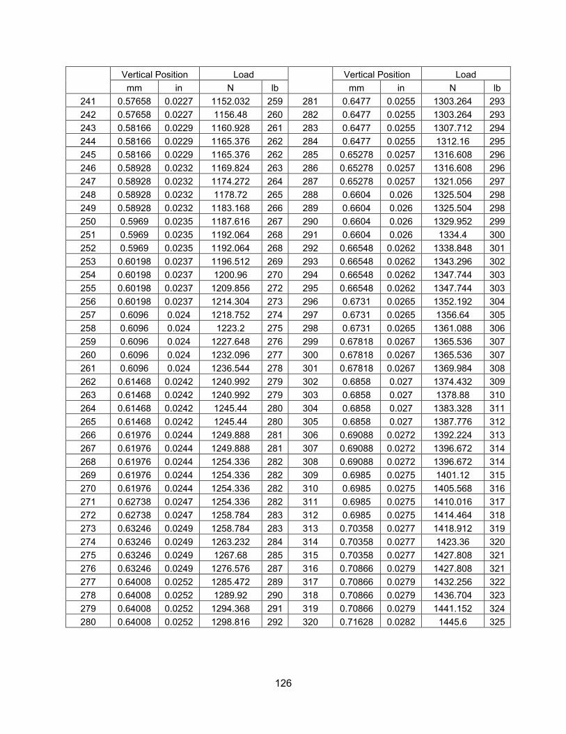
Vertical Position Load
Vertical Position Load
mm in N lb mm in N lb 241 0.57658 0.0227 1152.032 259 281 0.6477 0.0255 1303.264 293 242 0.57658 0.0227 1156.48 260 282 0.6477 0.0255 1303.264 293 243 0.58166 0.0229 1160.928 261 283 0.6477 0.0255 1307.712 294 244 0.58166 0.0229 1165.376 262 284 0.6477 0.0255 1312.16 295 245 0.58166 0.0229 1165.376 262 285 0.65278 0.0257 1316.608 296 246 0.58928 0.0232 1169.824 263 286 0.65278 0.0257 1316.608 296 247 0.58928 0.0232 1174.272 264 287 0.65278 0.0257 1321.056 297 248 0.58928 0.0232 1178.72 265 288 0.6604 0.026 1325.504 298 249 0.58928 0.0232 1183.168 266 289 0.6604 0.026 1325.504 298 250 0.5969 0.0235 1187.616 267 290 0.6604 0.026 1329.952 299 251 0.5969 0.0235 1192.064 268 291 0.6604 0.026 1334.4 300 252 0.5969 0.0235 1192.064 268 292 0.66548 0.0262 1338.848 301 253 0.60198 0.0237 1196.512 269 293 0.66548 0.0262 1343.296 302 254 0.60198 0.0237 1200.96 270 294 0.66548 0.0262 1347.744 303 255 0.60198 0.0237 1209.856 272 295 0.66548 0.0262 1347.744 303 256 0.60198 0.0237 1214.304 273 296 0.6731 0.0265 1352.192 304 257 0.6096 0.024 1218.752 274 297 0.6731 0.0265 1356.64 305 258 0.6096 0.024 1223.2 275 298 0.6731 0.0265 1361.088 306 259 0.6096 0.024 1227.648 276 299 0.67818 0.0267 1365.536 307 260 0.6096 0.024 1232.096 277 300 0.67818 0.0267 1365.536 307 261 0.6096 0.024 1236.544 278 301 0.67818 0.0267 1369.984 308 262 0.61468 0.0242 1240.992 279 302 0.6858 0.027 1374.432 309 263 0.61468 0.0242 1240.992 279 303 0.6858 0.027 1378.88 310 264 0.61468 0.0242 1245.44 280 304 0.6858 0.027 1383.328 311 265 0.61468 0.0242 1245.44 280 305 0.6858 0.027 1387.776 312 266 0.61976 0.0244 1249.888 281 306 0.69088 0.0272 1392.224 313 267 0.61976 0.0244 1249.888 281 307 0.69088 0.0272 1396.672 314 268 0.61976 0.0244 1254.336 282 308 0.69088 0.0272 1396.672 314 269 0.61976 0.0244 1254.336 282 309 0.6985 0.0275 1401.12 315 270 0.61976 0.0244 1254.336 282 310 0.6985 0.0275 1405.568 316 271 0.62738 0.0247 1254.336 282 311 0.6985 0.0275 1410.016 317 272 0.62738 0.0247 1258.784 283 312 0.6985 0.0275 1414.464 318 273 0.63246 0.0249 1258.784 283 313 0.70358 0.0277 1418.912 319 274 0.63246 0.0249 1263.232 284 314 0.70358 0.0277 1423.36 320 275 0.63246 0.0249 1267.68 285 315 0.70358 0.0277 1427.808 321 276 0.63246 0.0249 1276.576 287 316 0.70866 0.0279 1427.808 321 277 0.64008 0.0252 1285.472 289 317 0.70866 0.0279 1432.256 322 278 0.64008 0.0252 1289.92 290 318 0.70866 0.0279 1436.704 323 279 0.64008 0.0252 1294.368 291 319 0.70866 0.0279 1441.152 324 280 0.64008 0.0252 1298.816 292 320 0.71628 0.0282 1445.6 325
126
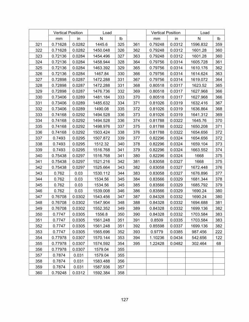
Vertical Position Load
Vertical Position Load
mm in N lb mm in N lb 321 0.71628 0.0282 1445.6 325 361 0.79248 0.0312 1596.832 359 322 0.71628 0.0282 1450.048 326 362 0.79248 0.0312 1601.28 360 323 0.72136 0.0284 1454.496 327 363 0.79248 0.0312 1601.28 360 324 0.72136 0.0284 1458.944 328 364 0.79756 0.0314 1605.728 361 325 0.72136 0.0284 1463.392 329 365 0.79756 0.0314 1610.176 362 326 0.72136 0.0284 1467.84 330 366 0.79756 0.0314 1614.624 363 327 0.72898 0.0287 1472.288 331 367 0.79756 0.0314 1619.072 364 328 0.72898 0.0287 1472.288 331 368 0.80518 0.0317 1623.52 365 329 0.72898 0.0287 1476.736 332 369 0.80518 0.0317 1627.968 366 330 0.73406 0.0289 1481.184 333 370 0.80518 0.0317 1627.968 366 331 0.73406 0.0289 1485.632 334 371 0.81026 0.0319 1632.416 367 332 0.73406 0.0289 1490.08 335 372 0.81026 0.0319 1636.864 368 333 0.74168 0.0292 1494.528 336 373 0.81026 0.0319 1641.312 369 334 0.74168 0.0292 1494.528 336 374 0.81788 0.0322 1645.76 370 335 0.74168 0.0292 1498.976 337 375 0.81788 0.0322 1650.208 371 336 0.74168 0.0292 1503.424 338 376 0.81788 0.0322 1654.656 372 337 0.7493 0.0295 1507.872 339 377 0.82296 0.0324 1654.656 372 338 0.7493 0.0295 1512.32 340 378 0.82296 0.0324 1659.104 373 339 0.7493 0.0295 1516.768 341 379 0.82296 0.0324 1663.552 374 340 0.75438 0.0297 1516.768 341 380 0.82296 0.0324 1668 375 341 0.75438 0.0297 1521.216 342 381 0.83058 0.0327 1668 375 342 0.75438 0.0297 1525.664 343 382 0.83058 0.0327 1672.448 376 343 0.762 0.03 1530.112 344 383 0.83058 0.0327 1676.896 377 344 0.762 0.03 1534.56 345 384 0.83566 0.0329 1681.344 378 345 0.762 0.03 1534.56 345 385 0.83566 0.0329 1685.792 379 346 0.762 0.03 1539.008 346 386 0.83566 0.0329 1690.24 380 347 0.76708 0.0302 1543.456 347 387 0.84328 0.0332 1690.24 380 348 0.76708 0.0302 1547.904 348 388 0.84328 0.0332 1694.688 381 349 0.76708 0.0302 1552.352 349 389 0.84328 0.0332 1699.136 382 350 0.7747 0.0305 1556.8 350 390 0.84328 0.0332 1703.584 383 351 0.7747 0.0305 1561.248 351 391 0.8509 0.0335 1703.584 383 352 0.7747 0.0305 1561.248 351 392 0.85598 0.0337 1699.136 382 353 0.7747 0.0305 1565.696 352 393 0.9779 0.0385 987.456 222 354 0.77978 0.0307 1570.144 353 394 1.10236 0.0434 542.656 122 355 0.77978 0.0307 1574.592 354 395 1.22428 0.0482 302.464 68 356 0.77978 0.0307 1579.04 355 357 0.7874 0.031 1579.04 355 358 0.7874 0.031 1583.488 356 359 0.7874 0.031 1587.936 357 360 0.79248 0.0312 1592.384 358
127