UNIVERSITY OF MASSACHUSETTS, AMHERST

DEPARTMENT OF PHYSICS

HONORS THESIS

Design, Construction, and Simulation ofMulti-Wire Proportional Chambers

for Charged Pion Polarizability Experiment at Jefferson Lab,Virginia

UMass Medium Energy Nuclear Physics

Bobby Johnston

Committee MembersProfessor Miskimen

Professor Kawall

June 1, 2017

AbstractThomas Jefferson National Accelerator Facility in Newport News, Virginia, will be running

an experiment to test a fundamental property of nature called the polarizability of the pion. This

property has a predicted value from the theory of Quantum Chromodynamics, which is the

leading theory describing the strong force, which is one of the four fundamental forces of nature.

In order to carry out this experiment, named the Charged Pion Polarizability Experiment at JLab,

requires a wide array of different particle detectors, each of which has a different purpose. One

set of these detectors, called Multi-Wire Proportional Chambers, have been set to be constructed

by the UMass Medium Energy Nuclear Physics lab. This paper details the design, construction,

and simulation of these detector prototypes and acts as a guide for future detector construction.

2

Contents

1 Introduction 3

2 Background 4

2.1 The Charged Pion Polarizability Experiment at JLab . . . . . . . . . . . . . . . . 4

2.2 UMass Amherst MENP Detector Development . . . . . . . . . . . . . . . . . . . 5

3 Background on Multi-Wire Proportional Chambers 6

3.1 Multi-Wire Proportional Chambers . . . . . . . . . . . . . . . . . . . . . . . . . . 6

3.2 Specific Design of CPP MWPC . . . . . . . . . . . . . . . . . . . . . . . . . . . 7

4 MWPC Electronics 8

4.1 Purpose of Electronics & Original Designs . . . . . . . . . . . . . . . . . . . . . . 8

4.2 Full-Scale Prototype & Testing . . . . . . . . . . . . . . . . . . . . . . . . . . . . 10

4.3 Modifications & Final Design . . . . . . . . . . . . . . . . . . . . . . . . . . . . 12

4.4 Development of Small Circuit End Boards . . . . . . . . . . . . . . . . . . . . . . 15

5 MWPC Prototypes - Small & Medium 17

5.1 Small Prototypes . . . . . . . . . . . . . . . . . . . . . . . . . . . . . . . . . . . 18

5.2 Medium Sized Prototype . . . . . . . . . . . . . . . . . . . . . . . . . . . . . . . 19

6 MWPC Prototypes - Full Scale 24

6.1 Preparing Detector Plates . . . . . . . . . . . . . . . . . . . . . . . . . . . . . . . 25

6.2 Stringing Detector Wires . . . . . . . . . . . . . . . . . . . . . . . . . . . . . . . 28

6.3 Detector Testing & Future Plans . . . . . . . . . . . . . . . . . . . . . . . . . . . 33

7 MWPC Simulation 34

7.1 Background to Geant4 . . . . . . . . . . . . . . . . . . . . . . . . . . . . . . . . 34

1

7.2 Simulations at JLab . . . . . . . . . . . . . . . . . . . . . . . . . . . . . . . . . . 37

7.3 Bringing Geant4 to UMass . . . . . . . . . . . . . . . . . . . . . . . . . . . . . . 43

7.4 Improvements to Simulation Structure . . . . . . . . . . . . . . . . . . . . . . . . 44

8 Conclusion 48

8.1 Future Works . . . . . . . . . . . . . . . . . . . . . . . . . . . . . . . . . . . . . 48

8.2 Acknowledgments . . . . . . . . . . . . . . . . . . . . . . . . . . . . . . . . . . 48

References 49

2

1 IntroductionFor the universe to exist as we know it, a fundamental symmetry of nature is necessary.

One way that engineers and physicists can test this symmetry is by measuring the polarizability

of pions. Pions are particles that mediate the strong nuclear force, which governs the binding of

the components that constitute basic blocks of matter such as protons and neutrons. All particles,

including pions, have fundamental properties such as polarizability, which is similar to charge or

mass. Quantum Chromodynamics (QCD), the current leading theory describing the strong force,

makes various predictions regarding physical phenomena, the most prominent being the polariz-

ability of the pion.

However, there have been significant issues in measuring this value, so much so that the sci-

entific community is unsure if the value agrees with the prediction made by QCD. An experiment

has been proposed to take place at the Thomas Jefferson National Accelerator Facility (JLab) in

Virginia to determine the polarizability with a proposed accuracy of 10%. This degree of accuracy

will lend enough statistical certainty to provide strong evidence for or against predictions of low

energy QCD. Figure 1 below shows a plot of the pion polarizability value as predicted by theory

(horizontal black line marked ChPT on vertical axis) and various experimentally measured val-

ues (shown with vertical bars indicating their respective standard deviations). The colors relate to

which experimental method was used. Only one experiment lies in agreement with theory (MARK

II), while the other six do not and do not even agree with each other.

Precisely measuring the value of the polarizability of the pion then provides a firm test to

quantum chromodynamics and the fundamental symmetries it describes. This thesis details the de-

velopment of one particular detector that is central to the success of this experiment, the Multi-Wire

Proportional Chamber, also referenced as the Muon Chambers - so named because their purpose

is to differentiate muons from pions in the experiment, as explained in the next sections.

3

Figure 1: Plot of pion polarizability values, from theory (black) and from experiment (colored) [1]

2 Background

2.1 The Charged Pion Polarizability Experiment at JLab

The Charged Pion Polarizability Experiment is a nuclear physics experiment taking place at

Jefferson Lab (JLab) in Newport News, Virginia to explore fundamental symmetries of nature. A

large amount of experimental hardware is required in order to conduct polarizability experiments

that accurately record the events occurring inside the particle accelerator, such as calorimeters,

which record the energy of passing particles, drift chambers, which register positional data, and

more. An illustration of the detector environment for this experiment at JLab is shown in Figure 2.

4

Figure 2: Scale illustration of the JLab Hall D setup for the CPP experiment [1]

Not shown in this figure are the Multi-Wire Proportional Chambers (MWPCs) which will

be installed behind the lead-glass calorimeter. Due to the physics behind the experiment, there will

be a large muon background to the pion signal, and there has to be a way to separate the signal

from the noise. This is where the MWPCs come in. At a basic level, the MWPCs will record all

ionizing particles that pass through it. The particles will then be directed through a thick sheet

of iron, at which point only muons can pass through. By placing another detector after this iron,

and backtracking through data, one can determine which particles are muons and which are pions

based off of what hits are registered in each MWPC.

2.2 UMass Amherst MENP Detector Development

In order to build these detectors, a number of smaller prototypes and one full-size prototype

have been developed over the past several years. As mentioned, this thesis details the design and

5

construction of all of these detectors, as well as the simulations and electronics for the MWPCs.

UMass MENP itself has designed similar chambers in the past [2] and with a fully functioning

clean room, is prepared to create more in the future.

3 Background on Multi-Wire Proportional

Chambers

3.1 Multi-Wire Proportional Chambers

On a basic level, a MWPC consists of many evenly spaced parallel wires mounted to a

rectangular enclosed frame filled with a specific gas composition containing argon and carbon

dioxide. Similar to a fly hitting a tennis racket and causing the strings to vibrate, a charged particle

hitting the wires on the MWPC causes a surge of current on the wires. This current can then be

detected and amplified by electronic circuits, and the data can be stored using software programs

for further analysis.

Figure 3 shows a cross sectional view of a MWPC. As an ionizing particle, here shown to

be a muon, passes through the detector, it ionizes gas atoms, freeing electrons. The electrons

avalanche towards the sense wire, where current develops.

6

Figure 3: Cross-sectional view of MWPC. Note the difference in diameters of sense and fieldwires, and their alternating pattern [3].

3.2 Specific Design of CPP MWPC

MWPCs allow for researchers to filter out unwanted particle data from the information about

the pions, which will then allow for calculations leading to a measure of its polarizability. Each

detector for the CPP experiment will measure 64 64 3 and have 144 sensing wires spaced exactly

0.4 apart. The wires will be electrically connected to an array of printed circuit boards (PCBs)

which will amplify the signal for data collection.

The process to build these full-scale detectors can be thought of as being broken up into

three phases. The first phase was carried out over the past few years by other members in my

research group. This portion of the research was focused on constructing small sized (1:8 scale)

inexpensive detectors that tested the general principles and basic sensing electronics. Tests were

conducted using sample radioactive sources such as iron-55 to generate current pulses on the wires.

Following this, medium and full size prototypes were constructed, and we are currently finishing

the full-scale detector testing. Figure 4 shows a more detailed schematic with details pertinent to

our exact detector.

7

inner ∅ 11mil,outer ∅ 28mil

Al0.6

43”

0.2”

∅ 50.8 μ𝑚

0.8

”

0.4

”

No offset

Exactly at the center

∅ 20 μ𝑚

Al

2.0

86”

Iron

Iron

1cm

1cm

Figure 4: Cross-sectional view of MWPC with details specific to detectors built by MENP. Theiron blocks on top and bottom of the detector will be installed along with the MWPCs in JLab

Parallel to these prototypes was the development of various prototypes of electronics for

amplifying the particle current signals, and developing software simulations of the MWPCs for the

CPP experiment. The following sections detail these respective parts of the lab research, although

one should keep in mind that they were all in work at the same time, with improvements and

realizations in one area affecting changes in others.

4 MWPC Electronics

4.1 Purpose of Electronics & Original Designs

As described previously, the MWPC has a set of electronics which act to amplify the electric

signals produced in the detector wires. Generally, the electronics function as an op-amp circuit

which magnifies the current signal in the wire to a voltage signal on the op-amp output, increasing

8

the signal magnitude by a factor of about 10,000. Preliminary work on this was initiated several

years ago by Christian Haughwout [3] and tested in the small scale MWPC prototypes (see section

5.1). By the time Christian had completed his undergraduate degree, the lab was ready to test

electronics on a medium sized MWPC with a printed circuit board (PCB) that was the full size of

what would be used on the full-scale MWPCs.

Figure 5: Preliminary amplification circuit as of Spring 2015 [3]

Figure 5 shows a schematic diagram of the circuit that was used for the medium sized

prototype build. For full details on the work behind this design, please refer the Christian’s thesis

[3]. The circuit board constructed for the medium sized MWPC had 24 of these amplification

circuits, one for each active channel in the detector. In summer 2015 the PCBs for this detector

were fabricated from the company Advanced Circuits, and board elements were populated by hand.

9

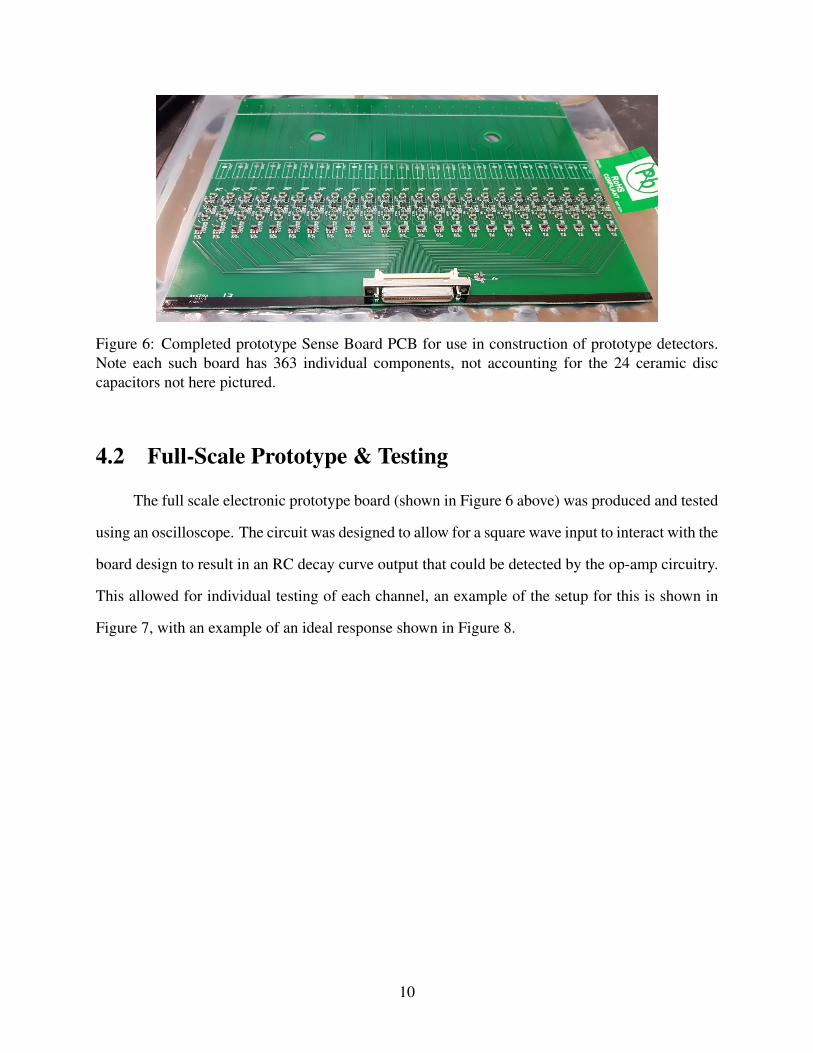
Figure 6: Completed prototype Sense Board PCB for use in construction of prototype detectors.Note each such board has 363 individual components, not accounting for the 24 ceramic disccapacitors not here pictured.

4.2 Full-Scale Prototype & Testing

The full scale electronic prototype board (shown in Figure 6 above) was produced and tested

using an oscilloscope. The circuit was designed to allow for a square wave input to interact with the

board design to result in an RC decay curve output that could be detected by the op-amp circuitry.

This allowed for individual testing of each channel, an example of the setup for this is shown in

Figure 7, with an example of an ideal response shown in Figure 8.

10

Figure 7: Example setup for electronics testing of PCBs

Figure 8: Example oscilloscope output from PCB transformers when testing boards using pulsescope driven with 1 Volt square wave at 50 % duty.

The medium sized MWPC prototype was designed to test one of these boards, and the

11

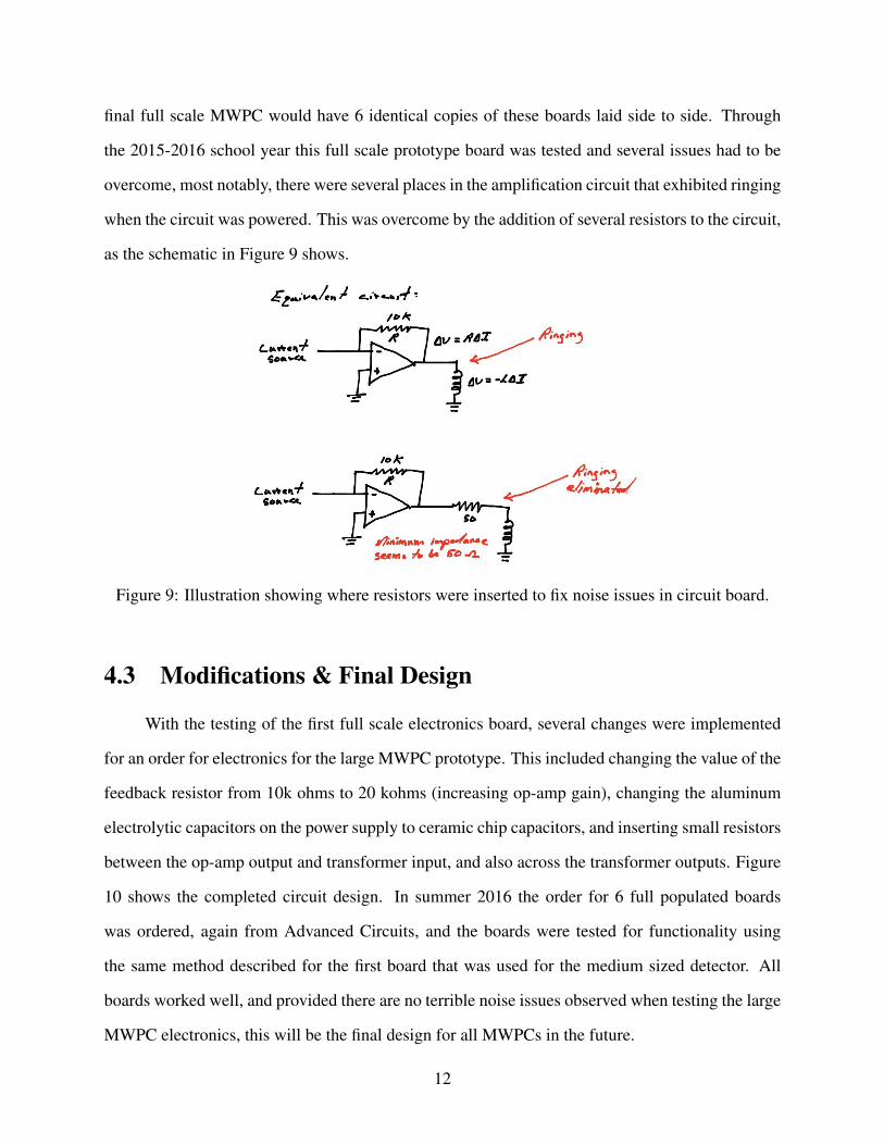
final full scale MWPC would have 6 identical copies of these boards laid side to side. Through

the 2015-2016 school year this full scale prototype board was tested and several issues had to be

overcome, most notably, there were several places in the amplification circuit that exhibited ringing

when the circuit was powered. This was overcome by the addition of several resistors to the circuit,

as the schematic in Figure 9 shows.

Figure 9: Illustration showing where resistors were inserted to fix noise issues in circuit board.

4.3 Modifications & Final Design

With the testing of the first full scale electronics board, several changes were implemented

for an order for electronics for the large MWPC prototype. This included changing the value of the

feedback resistor from 10k ohms to 20 kohms (increasing op-amp gain), changing the aluminum

electrolytic capacitors on the power supply to ceramic chip capacitors, and inserting small resistors

between the op-amp output and transformer input, and also across the transformer outputs. Figure

10 shows the completed circuit design. In summer 2016 the order for 6 full populated boards

was ordered, again from Advanced Circuits, and the boards were tested for functionality using

the same method described for the first board that was used for the medium sized detector. All

boards worked well, and provided there are no terrible noise issues observed when testing the large

MWPC electronics, this will be the final design for all MWPCs in the future.

12

Figure 10: Provisional finalized circuit schematic as of the beginning of May 2017. Refer to lablogbooks for completely finalized design as of July 2017.

With the circuit complete, we will now describe briefly how the circuit functions. Again,

for a full treatment and detailed analysis behind choices for electronic components, refer to Chris-

tian Haughwout’s thesis [3]. Starting from the bottom right of the schematic, we see a sense wire

which is biased at +2000 V. When an ionizing particle passes through the detector, it creates an

avalanche of electrons which collect on this wire and create a current signal. This signal passes

through the 47 uF DC blocking capacitor, which acts to remove the +2000 V bias. There are two

1N4184 diodes which act as clamps to ground; this is to protect the op-amp so that it never receives

an input voltage greater than 0.7 volts absolute. The current signal is then amplified by the op-amp

circuit by a factor of roughly 20k (set by the 20k ohm feedback resistor) and passes through a

10 ohm dampening resistor to a MABAE0060 transformer. The transformer changes the signal

from single ended to differential, which is what is required by the electronics systems in place at

Jefferson Lab. There is a 200 ohm resistor across the transformer output to further dampen ringing

effects in the circuit. Returning to the op-amp section of the circuit, there is a feedback resistor and

capacitor, which are basic op-amp elements. The op-amp is powered by a +5 V and -5 V current

source, which has capacitors to ground to quite the power supply.

As mentioned in the section discussing testing the electronics, there is also a pulse circuit in-

tegrated into each PCB. The circuit accepts a differential square wave input which passes through

13

a transformer to yield a single ended input. This input passes through a 5.1k resistor and to the un-

derside of the circuit board, where the board capacitance itself it utilized to produce an RC signal,

which is detected and amplified by the op-amp circuit for testing and calibration purposes. It is

important to not that the test input into the transformer must be truly differential (and not grounded

out) or else the circuit produces strange reflections and ringings that can be difficult to resolve.

Figure 11: Final circuit board design for Sense Board PCB.

These circuits were physically designed using the industry software CADSoft Eagle,

which has recently been acquired by the CAD company Autodesk and is now just called Eagle. The

software is relatively intuitive to learn, with the basics being that the red coloring indicates copper

traces on top of the circuit board, blue indicates bottom side copper traces, and green represents

through-holes and vias. Figure 11 shows the completed finalized circuit board design as seen in this

software environment. Figure 12 below shows the corresponding completed high-voltage biasing

board. Not much time was spent discussing this board as it has only one component (a 1M resistor)

and is very simple compared to the sense board, but it is included here for completeness.

14

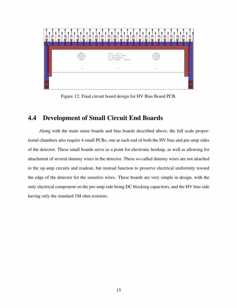
Figure 12: Final circuit board design for HV Bias Board PCB.

4.4 Development of Small Circuit End Boards

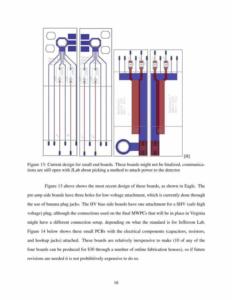
Along with the main sense boards and bias boards described above, the full scale propor-

tional chambers also require 4 small PCBs, one at each end of both the HV bias and pre-amp sides

of the detector. These small boards serve as a point for electronic hookup, as well as allowing for

attachment of several dummy wires in the detector. These so-called dummy wires are not attached

to the op-amp circuits and readout, but instead function to preserve electrical uniformity toward

the edge of the detector for the sensitive wires. These boards are very simple in design, with the

only electrical component on the pre-amp side being DC blocking capacitors, and the HV bias side

having only the standard 1M ohm resistors.

15

[H]

Figure 13: Current design for small end boards. These boards might not be finalized, communica-tions are still open with JLab about picking a method to attach power to the detector.

Figure 13 above shows the most recent design of these boards, as shown in Eagle. The

pre-amp side boards have three holes for low-voltage attachment, which is currently done through

the use of banana plug jacks. The HV bias side boards have one attachment for a SHV (safe high

voltage) plug, although the connections used on the final MWPCs that will be in place in Virginia

might have a different connection setup, depending on what the standard is for Jefferson Lab.

Figure 14 below shows these small PCBs with the electrical components (capacitors, resistors,

and hookup jacks) attached. These boards are relatively inexpensive to make (10 of any of the

four boards can be produced for $30 through a number of online fabrication houses), so if future

revisions are needed it is not prohibitively expensive to do so.

16

Figure 14: Physical products of the small end boards. Observe the red (+5V) white (-5V) and black(GND) banana plugs and SHV plug used for power attachments.

5 MWPC Prototypes - Small & MediumIt would not be the best idea to jump straight into construction of full size MWPCs without

first testing the design on smaller prototypes. The full-scale MWPCs will cost several thousands of

dollars to produce per detector, while smaller detector prototypes can be manufactured for much

cheaper, sometimes less than $100 per detector when they are very small. The purpose of these

detectors is to slowly move from computer designs and drawings to a full working detector. In

working with practical electronics, ideas can be worked out in theory as much as one desires,

but things will always be different when physically building the devices. There are simply far

too many variables to be completely thought of before production, especially when the desired

end product is both physically large and requires a very fine degree of precision. These MWPCs

satisfy both of these criteria, measuring about 6 feet by 6 feet by 4 inches in size, while requiring a

precision in many parts of less than a thousandth of an inch. This precision, spanning several orders

17

of magnitude, combined with the complications of several thousand of electronic components,

make for almost countless ways that critical mistakes can be made in designing and building these

detectors. If even one electronic component is placed in a location without proper thought, it could

completely hinder the entire function of the MWPC.

5.1 Small Prototypes

UMass MENP started small several years ago in designing small-scale MWPCs that mea-

sured about 6 inches by 6 inches square. These detectors were very cheap to make (less than $100

including electronics) - this was made possible due to the fact that the electronic circuit boards

were very small (PCB price scales very poorly with size due to fabrication method) and that the

frames of the detector, used for structural support, could be printed using the physics department’s

3D printer.

Figure 15 shows a top-down view of one such small sized detector with the top aluminum

plate removed. The white sides of the detector are the 3D printed frames, which are fabricated out

of ABS plastic, the same plastic used to create LEGOs. The black ring in the middle of the frame

is an O-ring rubber used to improve the air-tight property of the detector, which is held in using

very thin mylar tape. The circuit boards can be seen with the wires string across the two boards.

Only the field wires are visible, as the sense wires are too small to be visible at this scale. The

black line in the center is a carbon rod, which will be discussed further in future sections. These

small scale detectors were developed mainly during 2013 - 2015, with older members of the lab

doing the majority of this work. Full details can be found in honors theses written by Christian

Haughwout [3] and Andrew Schick [9].

18

Figure 15: One of the several small-size prototype MWPCs made in the lab.

5.2 Medium Sized Prototype

Following the success of several small scale MWPCs, a medium scale (1 foot by 1 foot) de-

tector was constructed. This detector was designed and constructed over the summer of 2016, and

at this scale was still amenable to 3D printing. As such, the 3D design program Autodesk Inventor

c©was used to design the plastic frames and aluminum plates for the detector. Figure 16 shows a

view of one of the detector frames, as seen in the Autodesk Inventor developer environment. Note

the groove which was designed for the O-ring rubber seal to sit in, and the depressed areas to allow

room for the electronic circuit boards to sit in.

19

Figure 16: CAD rendering of plastic spacer frame.

The aluminum plates were also designed using this software, and were of even simpler

design, consisting of a sheet of metal with 12 counter-sunk holes for screw attachments. Figure 17

shows the dimensions of the top such plate, again as seen in the developer environment. Unfortu-

nately, the plastic frames were too large to be printed on campus (most 3D printers have a build

area of no larger than 8 inches by 8 inches), so an online 3D printing company, Purple Platapus

c©was used to purchase the frames. These were relatively expensive at $300 for both frames, but

3D printing scales very poorly with increasing size of solid components. The aluminum plates

were also procured from a 3rd party vendor, but as it was such a simple design cost only somewhat

more than $100.

20

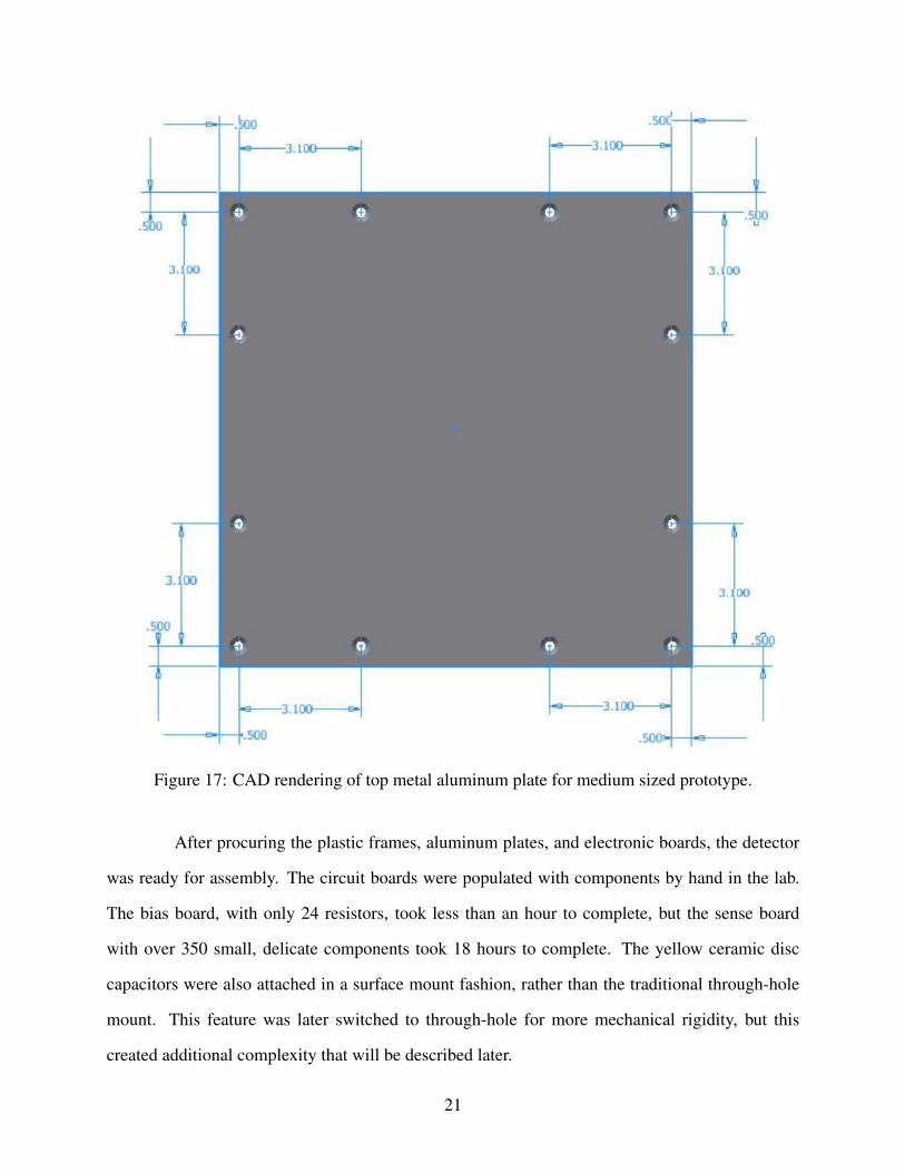
Figure 17: CAD rendering of top metal aluminum plate for medium sized prototype.

After procuring the plastic frames, aluminum plates, and electronic boards, the detector

was ready for assembly. The circuit boards were populated with components by hand in the lab.

The bias board, with only 24 resistors, took less than an hour to complete, but the sense board

with over 350 small, delicate components took 18 hours to complete. The yellow ceramic disc

capacitors were also attached in a surface mount fashion, rather than the traditional through-hole

mount. This feature was later switched to through-hole for more mechanical rigidity, but this

created additional complexity that will be described later.

21

To string the wires in the detector, the following method was used. Although the pad spacing

in the PCB design for the wires is 0.4 inches, there is an unreliable amount of precision due to

differing manufacturing tolerances in the world of circuit board manufacturing. Moreover, when

having 6 circuit boards end to end, as in the final MWPC design, small defects on each board

can propagate to large differences over the whole MWPC. For that reason, a more reliable method

of positioning wires is needed. For these detectors, long threaded rods were used as positioning

devices, which typically have drifts of only a few mils over the whole length of the rod. Figure 18

illustrates how using a threaded rod was useful for positioning these wires.

Figure 18: Illustration of method to ensure precision in wire stringing.

Figure 19 below further illustrates the concept, with the wooden frame bracing visible.

Through this method wires were strung, and the same concept would be again applied for the large

MWPC prototype stringing, as described later.

22

Figure 19: Brace and rod used for wire stringing on medium detector.

The detector was strung with wires, as can be seen in Figure 20. The detector was large enough

to house one full scale sense PCB, which has 24 active channels. Again, the full-scale MWPC was

designed to have 6 of these PCBs for 144 active channels, with a small number of inactive dummy

wires along the edges of the detector.

Figure 20: Medium sized detector with stringing completed.

23

The detector was then closed and gas ports were added to facilitate the flow of the Argon

and CO2 gas used when the detector is operating. Wires were soldered to the detector for LV

power on the sense board, and HV biasing on the bias board. Additionally, wires were attached to

connect the sense board ground, bias board ground, and both aluminum plates together. Without

these attachments there would be ground loops in the detector and the electronics would respond

erratically. These wires (black wire) and gas ports (blue tubes) can be seen in Figure 21.

Figure 21: Medium MWPC with gas ports and grounding. The detector is at this stage completed.

6 MWPC Prototypes - Full ScaleThe last task before constructing the final versions of the full-scale MWPCs was to design

and build a full-scale prototype. This would be designed as though it were the final version, but

with the understanding that there would almost certainly be some oversights. With this in mind,

only one such prototype was produced - this means the single prototype is more expensive to

24

produce than a detector if 8 were manufactured at once, but in the long term this saves money as if

there are any errors it would be time consuming, if not impossible, to rectify the situation on all 8

detectors.

6.1 Preparing Detector Plates

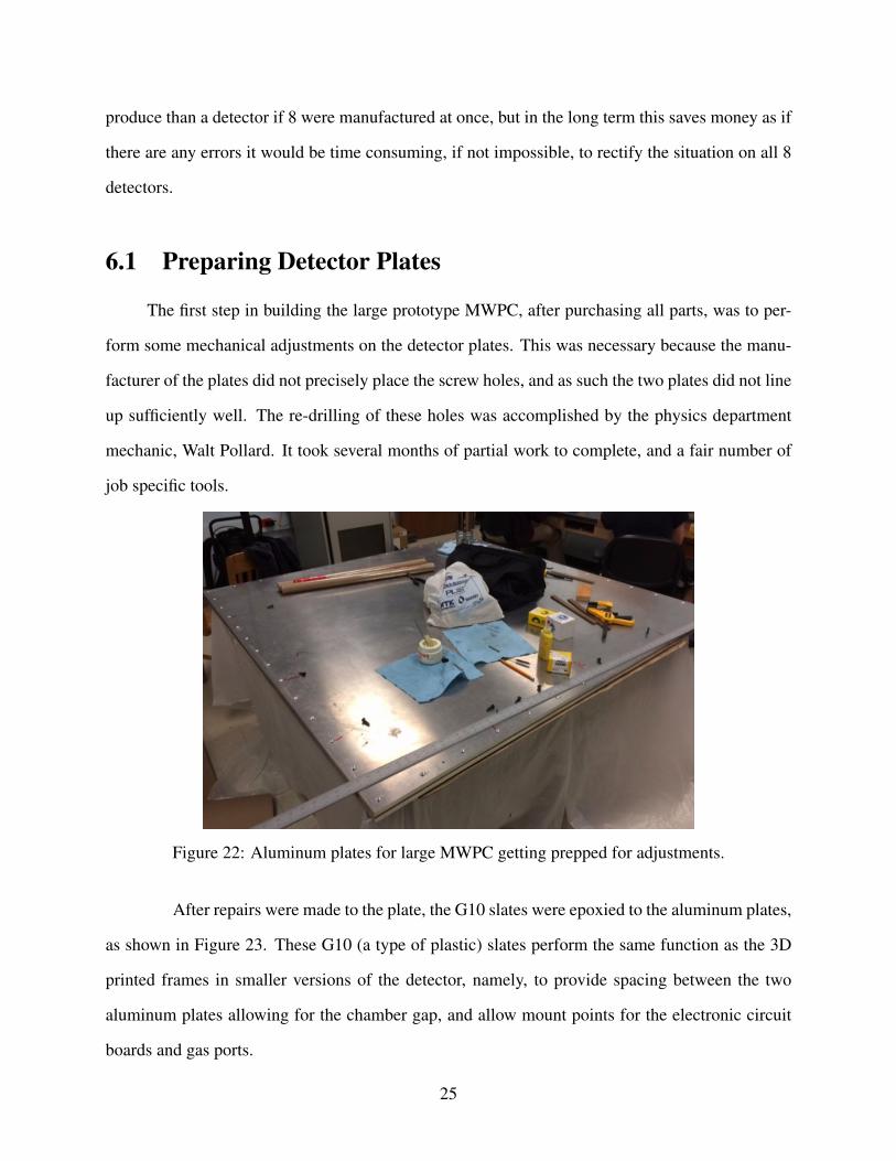
The first step in building the large prototype MWPC, after purchasing all parts, was to per-

form some mechanical adjustments on the detector plates. This was necessary because the manu-

facturer of the plates did not precisely place the screw holes, and as such the two plates did not line

up sufficiently well. The re-drilling of these holes was accomplished by the physics department

mechanic, Walt Pollard. It took several months of partial work to complete, and a fair number of

job specific tools.

Figure 22: Aluminum plates for large MWPC getting prepped for adjustments.

After repairs were made to the plate, the G10 slates were epoxied to the aluminum plates,

as shown in Figure 23. These G10 (a type of plastic) slates perform the same function as the 3D

printed frames in smaller versions of the detector, namely, to provide spacing between the two

aluminum plates allowing for the chamber gap, and allow mount points for the electronic circuit

boards and gas ports.

25

Figure 23: Aluminum plates and G10 plastic slats being epoxied together with the aid of clamps.

Before epoxying the PCBs to the G10 slats, the boards needed to be sanded down to

be able to all fit within the alloted area. Although the PCBs were manufactured with a nominal

width of 9.6 inches, no process is perfect and the boards were actually slightly oversized. By

careful sanding, several mils were removed from each board, such that all boards were able to

snugly fit within the space on the G10. Although only a few mils were removed on each board, the

cumulative total material removed was more than 50 mils, which is a very significant difference.

One should note that FR-54, the fiberglass material that PCBs are made from, are not particularly

benign, and proper PPE should be worn when sanding, particularly eye goggles and an N-95 or

better breathing mask.

26

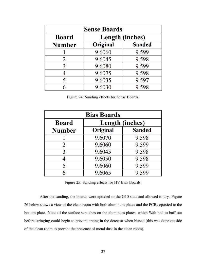
Figure 24: Sanding effects for Sense Boards.

Figure 25: Sanding effects for HV Bias Boards.

After the sanding, the boards were epoxied to the G10 slats and allowed to dry. Figure

26 below shows a view of the clean room with both aluminum plates and the PCBs epoxied to the

bottom plate. Note all the surface scratches on the aluminum plates, which Walt had to buff out

before stringing could begin to prevent arcing in the detector when biased (this was done outside

of the clean room to prevent the presence of metal dust in the clean room).

27

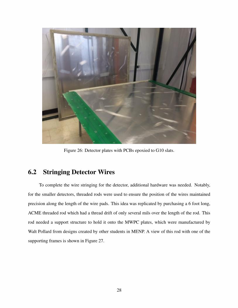
Figure 26: Detector plates with PCBs epoxied to G10 slats.

6.2 Stringing Detector Wires

To complete the wire stringing for the detector, additional hardware was needed. Notably,

for the smaller detectors, threaded rods were used to ensure the position of the wires maintained

precision along the length of the wire pads. This idea was replicated by purchasing a 6 foot long,

ACME threaded rod which had a thread drift of only several mils over the length of the rod. This

rod needed a support structure to hold it onto the MWPC plates, which were manufactured by

Walt Pollard from designs created by other students in MENP. A view of this rod with one of the

supporting frames is shown in Figure 27.

28

Figure 27: View of detector stringing with ACME rod and support structure in center top of image.Hanging from a non-visible wire is a clamp used to provide tension.

With this rod in place, the detector was ready to be strung. 3 wires were strung, without

soldering to pads, on the left, center, and rightmost regions of the detector. The purpose of these

wires was to calibrate the positioning of the rod, as well as ensure that throughout the process

of stringing, no bumping or changes to the detector set-up went unnoticed. Figure 28 shows the

detector set-up at this stage.

29

Figure 28: View of detector stringing with positioning wires in place (left, center, and right mostpads).

For the stringing, the methodology was to string the central region first, then move out-

wards to the left and right to finish stringing. Comprehensive details, in an instructional format,

can be found in Jordan Kornfeld’s thesis [8], as well as in a 60 slide long PowerPoint detailing

exact steps for stringing [10] that was created along with this thesis manuscript.

One point of interest is that stringing in the central region is complicated by the use of carbon

rods. These rods surround the sense wires to effectively increase the diameter of the sense wire,

which effectively deadens the wire in that region for detecting charged particles. The purpose of

having a dead region in the central region of the detector is to quiet it out so that the high beam

rate near the beam line does not drown out true signal hits. Figure 29 shows one such carbon rod,

30

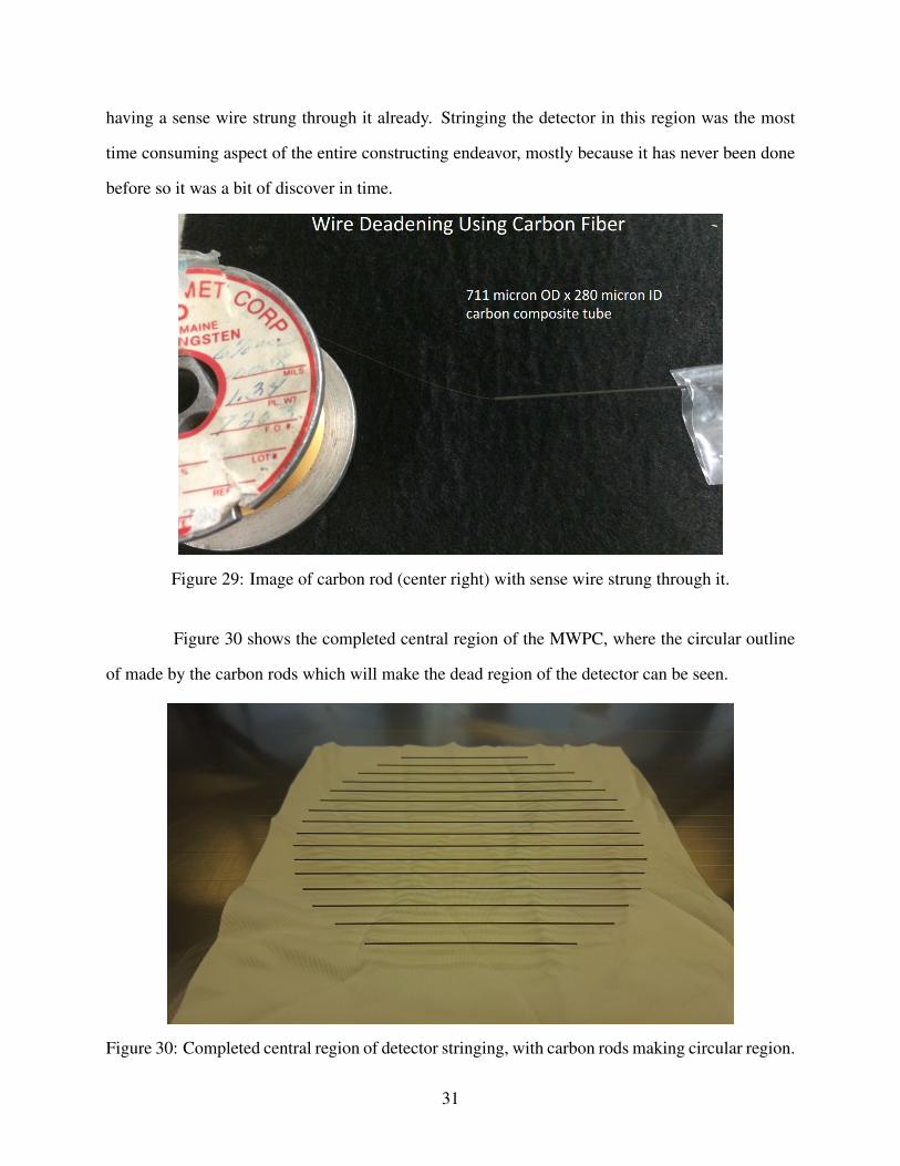
having a sense wire strung through it already. Stringing the detector in this region was the most

time consuming aspect of the entire constructing endeavor, mostly because it has never been done

before so it was a bit of discover in time.

Figure 29: Image of carbon rod (center right) with sense wire strung through it.

Figure 30 shows the completed central region of the MWPC, where the circular outline

of made by the carbon rods which will make the dead region of the detector can be seen.

Figure 30: Completed central region of detector stringing, with carbon rods making circular region.

31

Upon completion of the central region, the rest of the detector was strung. Some difficul-

ties were encountered, which are detailed in aforereferenced documents. On average, each string

took about 4 minutes to string, with sense wires taking about 5 and field wires taking about 3.

Overall, this corresponded to more than 1000 minutes of stringing along, without regard to set-up

time, clean up time everyday, or the entire central region, which took a few weeks on its own to

complete.

Figure 31: Myself (center) and Jordan Kornfeld (right) stringing wires.

After nearly 2 months of work, the MWPC stringing was completed. By shining a light in

a dark clean room, the wires are illuminated, showing evidence of the 300 wires that are otherwise

very difficult to see at a distance with the naked eye. Figure 32 shows the detector with completed

stringing.

32

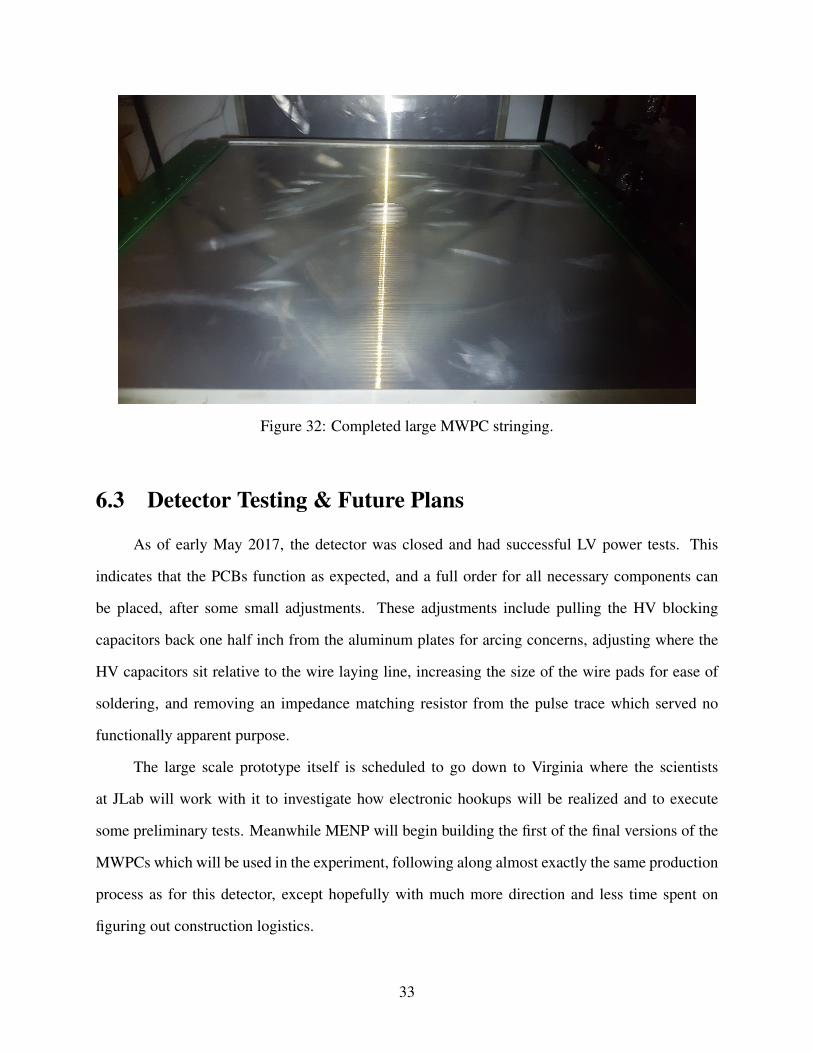
Figure 32: Completed large MWPC stringing.

6.3 Detector Testing & Future Plans

As of early May 2017, the detector was closed and had successful LV power tests. This

indicates that the PCBs function as expected, and a full order for all necessary components can

be placed, after some small adjustments. These adjustments include pulling the HV blocking

capacitors back one half inch from the aluminum plates for arcing concerns, adjusting where the

HV capacitors sit relative to the wire laying line, increasing the size of the wire pads for ease of

soldering, and removing an impedance matching resistor from the pulse trace which served no

functionally apparent purpose.

The large scale prototype itself is scheduled to go down to Virginia where the scientists

at JLab will work with it to investigate how electronic hookups will be realized and to execute

some preliminary tests. Meanwhile MENP will begin building the first of the final versions of the

MWPCs which will be used in the experiment, following along almost exactly the same production

process as for this detector, except hopefully with much more direction and less time spent on

figuring out construction logistics.

33

7 MWPC Simulation

7.1 Background to Geant4

Geant4 is the latest version of a set of simulation packages for modeling particle interac-

tions. Geant (GEometry ANd Tracking) was initally developed several decades ago by researchers

at Stanford and is completely open source [6]. It was designed for simulations of particle interac-

tions in various areas of science, most notably particle physics and the medical field. It is also used

by CERN scientists working at the LHC in Geneva, Switzerland [5]. It is the most comprehensive

and accurate particle simulation toolkit currently available, and as such it proves to be a very useful

tool for nuclear and particle physics experiment simulations.

As the MWPCs are very expensive to build, and the CPP experiment in general is extremely

resources intensive, it is worth it many times over to simulate various aspects of the experiment

using Geant4. Scientists at JLab have built software that reconstructs nearly all of the JLab accel-

erator facility and detector halls, including the new GlueX update in HallD. However, there was

not much work done to develop and simulate the MWPCs in this Geant4 environment. The main

goal of using the simulation to model the MWPCs was to investigate how effective they will be in

aiding to differentiate between muons and pions in the actual experiment.

As it costs essentially nothing to run a simulation (neglecting hardware costs and developer

time), a number of different detector geometries can also be simulated to find the optimal layout

for particle identification. This aspect of the research was initiated by scientists at Jefferson Lab

around 2010, but intensive work on it at UMass MENP began in spring of 2016. All work before

spring 16 is summarized through online logs from JLab, and can be pursued further as detailed in

the references [7].

Geant4 itself is a software program written in C++ but utilizes a number of different pack-

ages and languages to build a functioning simulation environment. This will be explained further

in the next section, but for now we can observe the products of the simulation. Figures 33 and ??

34

shows simulation runs of 2 muons and 2 pions, respectively, traveling through various detectors

and absorbing material. We can see that the muons mostly pass through the material, while the

pions shower and create a large number of particles. Each particle has a different track color, with

light green symbolizing electrons and other colors representing charges (positive or negative) on

the incident particles.

Figure 33: Muon events passing through Geant4.

Figure 34: Pion events passing through Geant4.

35

While looking at the simulation results in this manner is no doubt fascinating, the true

power of the Geant4 simulation comes in estimating the efficiency of the detectors for the CPP

experiment. As mentioned, the main purpose of the MWPCs is to differentiate between muons

and pions - an ideal system would be able to have perfect differentiation, such that all muon events

could be identified and eliminated while all pion events are identified and retained. In other words,

the ideal goal would be to reject 100 % of muon events while accepting 100 % of pion events. In

reality, nothing can be completely perfect, but it is the job of the MWPCs to try and make these

ratios as ideal as possible. To quantify this, we arrive at plots such as that shown in Figure 35

which shows a generic curve for background (muon) rejection ratio vs. signal (pion) acceptance.

The goal of changing number and geometry of MWPCs in the simulation was to see how it would

affect this figure of merit. As it currently stands in this figure, if 90 % of pion events were to be

accepted, 15 % of muon events would have to be accepted as well. With certain geometries, this

ratio can be greatly improved, as discussed in future sections here as well as in Jordan Kornfield’s

thesis [8].

36

Figure 35: Plot of Background Rejection vs. Signal Efficiency, created using Boosted DecisionTree Multi-Variate Analysis, a method of machine learning.

7.2 Simulations at JLab

In summer 2016 I went to Jefferson Lab for a period of 6 weeks with the goals of installing,

learning, and applying the Geant4 simulation structure to problems related to the MWPC design

for the MENP lab. The entire framework for running Geant4 is in itself a very complex network

of communicating programs, scripts, and other executables, as the flowchart on the following page

illustrates.

37

Overview ofCPPsimProcesses

Event Generation

- gen_2mu- Particle gun

CPP Simulation

- Geant4- hdds/xml files

- mcsmear

Simulation Reconstruction

- sim-recon- hd_root

- ccdb

Data Presentation & Analysis

-Root

Multi-Variate Analysis

- TMVA- cppmva

- Root

AdditionalSoftware Used

-Xerces-C-Jana

-MySQL-ccdb

-cernlib-clhep-others

CPP Simulation

- Geant4- hdds/xml files

- mcsmear

Event Generation

- gen_2mu- Particle gun

Simulation Reconstruction

- sim-recon- hd_root

- ccdb

38

Running the simulation is not as simple as it might seem; in Windows or Mac operating

systems one can simply download a program, click install, and run it in a matter of minutes. With

Linux operating systems and programs running on linux, the procedure is much more complex,

especially to the newly initiated, and moreover when so many programs need to be installed. A

guide to starting up Geant4 and CPPsim is fairly well documented online [6] but even with this

documentation and the help of JLab staff, it took me about a week before the entire system was

running properly.

After finagling with the system, everything worked properly and the simulation could be ran

as intended. Most of the environment was already developed, and one could straightforwardly

produce plots of the entire Hall D simulation in Jefferson Lab by running the simulation with the

command ./CPPsim -i (–interactive), as shown in Figure 36.

Figure 36: Overview of detector hall in Geant4.

Figure 37 shows a close up view of the environment, with visible particle tracks running

through the detectors. For orientation purposes, the large cylindrical object on the left of the image

is the solenoid which produces the magnetic field for the experiment and contains the central drift

39

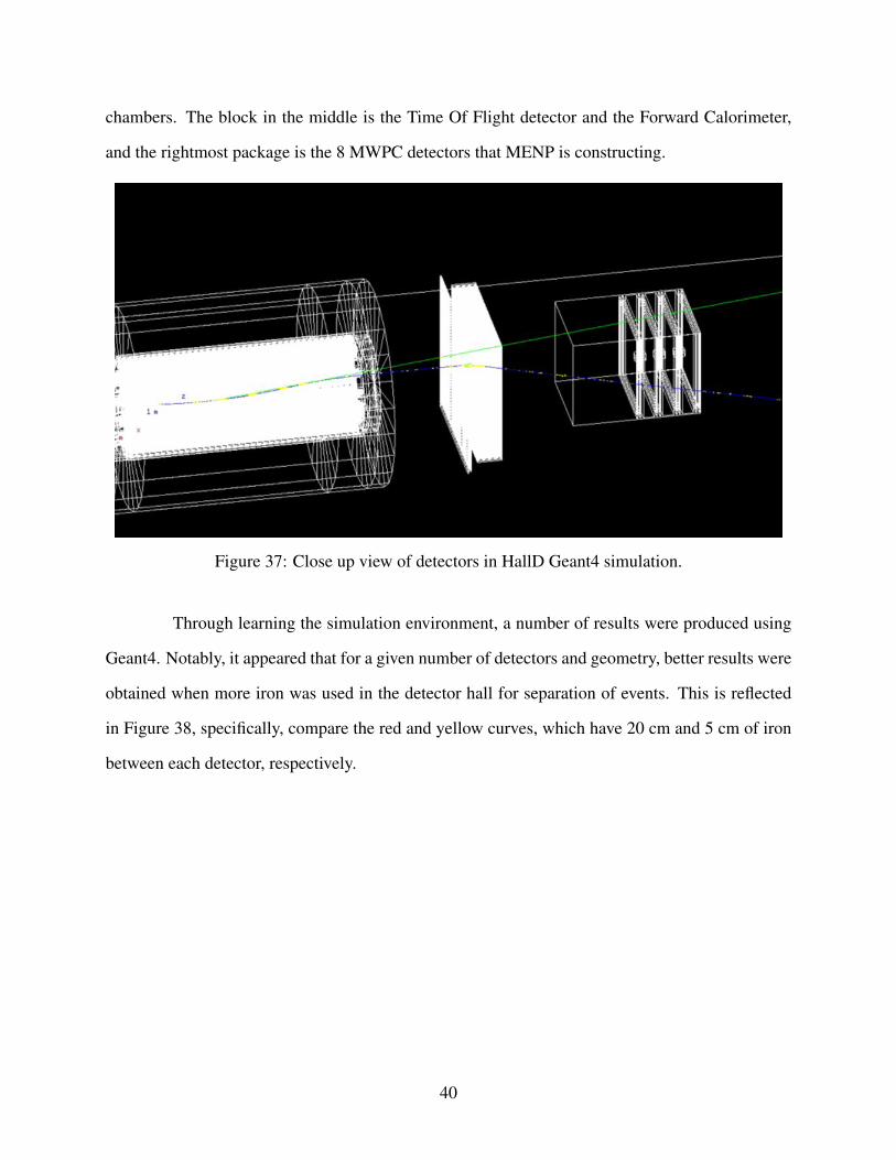
chambers. The block in the middle is the Time Of Flight detector and the Forward Calorimeter,

and the rightmost package is the 8 MWPC detectors that MENP is constructing.

Figure 37: Close up view of detectors in HallD Geant4 simulation.

Through learning the simulation environment, a number of results were produced using

Geant4. Notably, it appeared that for a given number of detectors and geometry, better results were

obtained when more iron was used in the detector hall for separation of events. This is reflected

in Figure 38, specifically, compare the red and yellow curves, which have 20 cm and 5 cm of iron

between each detector, respectively.

40

Figure 38: Simulation result showing effect of changing thickness of iron between detectors.

Also explored was how the number of MWPCs for a fixed amount of iron affects the

ability to differentiate between pions and muons. Figure 39 suggests an answer to this quesiton:

there is a very stark difference between 2, 4, and 6 detectors, but beyond 8 detectors there seems

to be a bit of information saturation and there is no additional benefit.

41

Figure 39: Effect of changing number of MWPCs in detector with a constant 20 cm of iron betweeneach detector.

Additionally, investigations were made into how changing energy minimum cutoffs for

input events affected separation of particles. The results showed a sharp falloff below a 4 GeV

minimum, as illustrated by Figure 40.

42

Figure 40: Effect of changing minimum energy cutoff limits on events in simulation.

7.3 Bringing Geant4 to UMass

After learning Geant4 and related simulation software at Jefferson Lab, it was decided that it

would be a very useful tool for MENP lab to have a working version of the entire simulation sys-

tem at UMass in LGRT. This has a number of benefits, the most obvious of which is that MENP

has access to any simulation results that could be needed, rather than having all information stored

on my personal laptop. Moreover, future students will be able to learn how to use Geant4, ROOT,

and other systems through MENP, which is a very rare opportunity that is usually only provided to

students in graduate school. Also, the computational power of a desktop dedicated to simulation is

likely stronger than that of a virtual machine on a personal laptop, and so simulations can include

more datasets and process results faster.

The first step to do this was to purchase a new computer for the lab. It couldn’t be extraor-

dinarily expensive, so a working limit of around $1000 was set aside for the desktop tower. This

43

allowed for the purchase of a relatively strong i7 quad-core processor, which, combined with hy-

perthreading, allowed for 8 virtual threads, which vastly improved computational power compared

to my laptop machine, which had only one core available for Geant4 simulations. The computer

also has 16 GB of RAM which further improves operational speeds. The other components of the

computer are fairly standard for a Dell Optiplex model, and function at the level necessary for the

lab’s tasks.

The next step was to install a working version of Linux Centos7, which is compatible with

the software needed to run the simulations. This was relatively straightforward, and from here we

could begin installing all software necessary to run Geant4 in the CPPsim environment. This was,

as always, quite a tedious task. One of the creators of Geant4 once joked in a seminar I attended

that ”The hardest part about Geant4, is installing Geant4“ and after going through two complete

installations, that certainly seems to be the case. Unfortunately there is not much I can write about

the steps to do this more easily, each individual computer has its own problems and will need indi-

vidual troubleshooting to arrive at a complete working installation, I will only say that Google and

Stack Overflow, and a large amount of persistence are the only tools to success.

Following the complete install of all necessary software, I began teaching Jordan how to

run and operate the simulation system to produce results. Again, please refer to his thesis [8] for

more details on his work, or observe logs written on the Dell lab computer for more information.

Finally, I will note that I tried to enable remote logins for the system with the vision that any

sufficiently motivated student could have access to particle physics simulations at UMass, but the

comprehensive system of firewalls did not allow this at the time of writing this.

7.4 Improvements to Simulation Structure

Once Geant4 was fully up and running on the MENP lab computer, simulation tasks were di-

rected to Jordan Kornfield, who details his work deeply in his thesis[8]. While he was handling the

main simulation functionality of the CPPsim Geant4 framework, there were a number of smaller

details that needed to be ironed out in the software structure to yield a more realistic simulation.

44

One such detail was to implement a virtual dead region in the MWPCs to simulate the car-

bon rods that are attached to the physical MWPCs which deaden the wires, as described previously.

Again, the main purpose of deadening these wires is to reduce the count rate in the central region,

as the count rate would otherwise be prohibitively high due to being so close to the beam line.

Figure 41 illustrates this high rate well - note the increasing number of hits as the wire approaches

the central region.

Figure 41: Left: Wire hits on all MWPCs without a dead region. Right: Wire hits on all MWPCswith a dead region. Note that hits do not go to zero on central region, but does drop dramatically.

Although the most rigorous approach would be to code in the carbon tubes onto each

individual sense wire in the simulation, this would be a very difficult and time consuming approach

without returning much value. Instead, code was written to neglect any particle hits in the MWPC

within a certain radius of the center. With this change to the code structure, a specified disc on the

MWPCs have exactly no hits, while the result of the detector is unchanged, as shown in Figure 42.

45

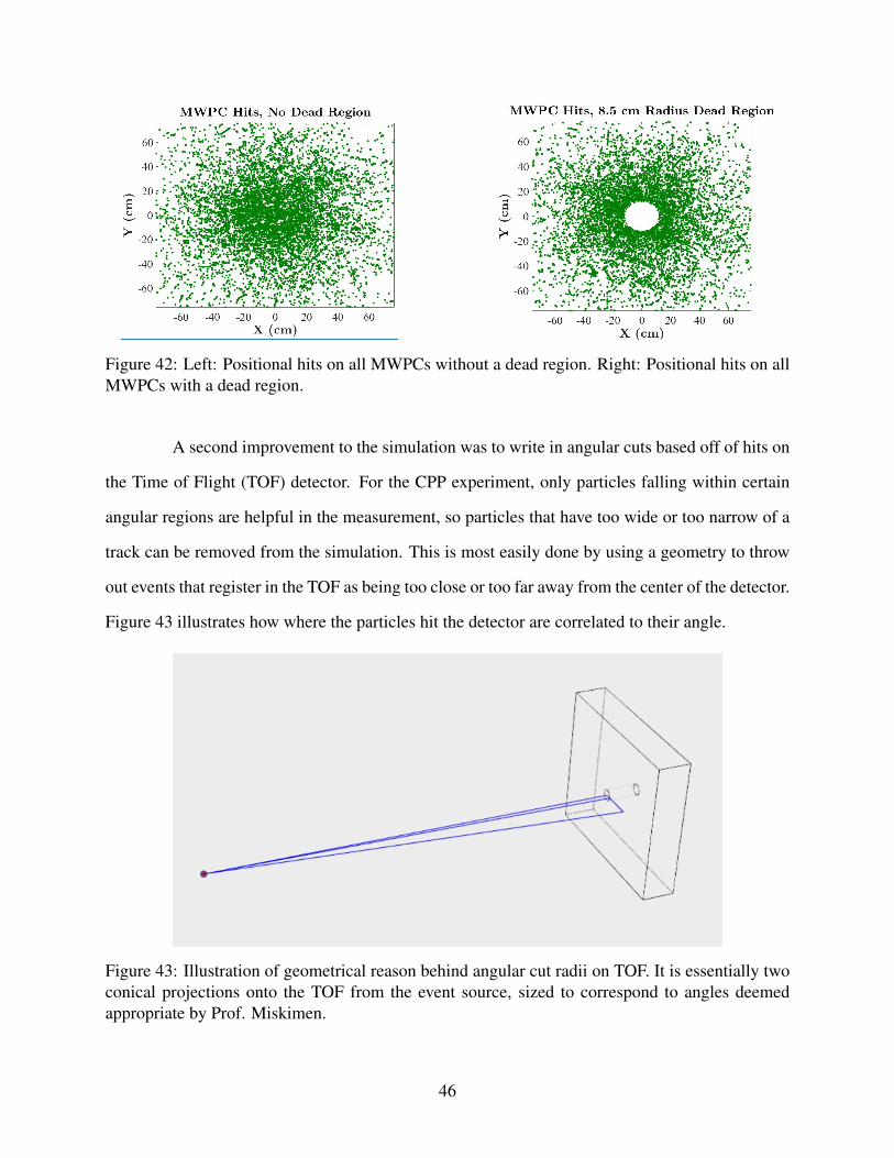
Figure 42: Left: Positional hits on all MWPCs without a dead region. Right: Positional hits on allMWPCs with a dead region.

A second improvement to the simulation was to write in angular cuts based off of hits on

the Time of Flight (TOF) detector. For the CPP experiment, only particles falling within certain

angular regions are helpful in the measurement, so particles that have too wide or too narrow of a

track can be removed from the simulation. This is most easily done by using a geometry to throw

out events that register in the TOF as being too close or too far away from the center of the detector.

Figure 43 illustrates how where the particles hit the detector are correlated to their angle.

Figure 43: Illustration of geometrical reason behind angular cut radii on TOF. It is essentially twoconical projections onto the TOF from the event source, sized to correspond to angles deemedappropriate by Prof. Miskimen.

46

In a straightforward way, the source code detailing the TOF detector hits was altered to

reject events that fell within or outside of certain cutoff regions, determined by Hall D geometry.

This is a bit more complex than the MWPC deadening as entire events must be rejected, not just

individual hits, and as so required a change to the entire CPPsim source. Results are shown in

Figure 44.

Figure 44: Hits on Time of Flight detector without (left) and with (right) angular cuts on detector.Note that there is already a dead region (square) in the time of flight to begin with.

While improvements were made, there is still a large amount of code upgrades that could

be considered. Rather than cutting angles using the TOF and implementing a dead region on the

MWPCs at the source code level, these improvements could be written in at the final analysis

step. This has a notable advantage in that in order to change the angular cuts or dead region size,

the entire CPPsim program must be rebuilt and recompiled, whereas if they were instituted at the

analysis level, the simulation would only have to be run once and could be analyzed with a variety

of parameters. Implementing this would require advanced C++ knowledge and would be a more

elegant solution, but both methods are functionally equivalent.

47

8 Conclusion

8.1 Future Works

Moving forward, the large scale MWPC prototype is set to travel down to Virginia sometime

in summer 2017 to be installed at Jefferson Lab. Following the conclusion of some simulation

results, full orders can be placed for detector plates and electronics. The final number of detec-

tors to be built is still open to discussion, and will be decided based off results of the simulation.

The design for the electronic boards are essentially entirely completed successfully, and will be

fabricated and assembled once a final number of detectors is decided upon. Conveniently, approxi-

mately every 2 weeks there is a Charged Pion Polarizability meeting which takes place in a virtual

meeting room. Slides and notes from these meetings are maintained through a wikipedia logbook,

and serve as an excellent place to see what has and currently is happened with the CPP experiment,

both at JLab and UMass MENP [11].

8.2 Acknowledgments

The work outlined in this thesis would in no way be possible without the help of almost

countless individuals and organizations. Above all, I would thank Professor Miskimen for bringing

me onto this project, and taking the chance with me even though I had no direct skills whatsoever at

the time of hire. Additionally, I would like to thank Christian Haughwout, upon which so much of

my work was based, for not only outlining my direction but also pushing me into the lab in the first

place, I certainly wouldn’t be writing this without his advice several years ago to join a lab group.

Beyond this, I sincerely thank all of the other members of MENP and the CPP experiment at JLab

that have helped me so much: David Lawrence, Elton Smith, Ilya Larin, Andrew Schick, Sean

McGrath, Matt Downing, Jordan Kornfeld, and all the other individuals who are too numerous for

me to mention individually.

48

References

[1] R. Miskimen, et al. “Measuring the Charged Pion Polarizability in the γγ → π+π− Reaction”Proposal for JLab PAC40, Ref: PR12-13-008, 2013.

[2] E. L. Foley, “The Design and Construction of a New VCDX Drift Chamber” UndergraduateHonors Thesis, University of Massachusetts, Amherst, MA, May 1998.

[3] C. A. Haughwout, “Design and Prototyping of MWPC Preamp Electronics for use in theCharged Pion Polarizability Experiment at Jefferson Lab” Undergraduate Honors Thesis, Uni-versity of Massachusetts, Amherst, MA, May 2015

[4] F. Sauli, “Principles of operation of multi wire proportional and drift chambers” CERN 68-79.1977.

[5] S. Agostinelli, et al. “Geant4 - A Simulation Toolkit” Nuclear Instruments and Methods inPhysics Research, 2003, 250-303

[6] A. Morsch et. al. “Geant4 Users Forum” Web. Last Updated May 27 2017.http://www.geant4.org/geant4/

[7] D. Lawerence, “CPPSim” Web.July 5 2016. https://halldweb.jlab.org/wiki/index.php/CPPsim

[8] J. S. Kornfeld, “Jefferson National Laboratory Charged Pion Polarizablity Experiment: MonteCarlo Simulation Using Geant4 and Construction of Multi-Wire Proportional Chambers” Un-dergraduate Honors Thesis, University of Massachusetts, Amherst, MA, May 2017

[9] A. Schick, “Developing Methods for Measuring the Pion Polarizability” Undergraduate Hon-ors Thesis, University of Massachusetts, Amherst, MA, December 2016

[10] R. Johnston, J. S. Kornfeld “How to String a Large MWPC” Document produced for labreference. University of Massachusetts, Amherst, MA, April 2017

[11] R. Miskimen, D. Lawerence, E. Smith, I. Larin, et. al. “Pion Polarizability Meetings” Web.Last data log May 19 2017. https://halldweb.jlab.org/wiki/index.php/

49