design, construction, and evaluation of low-cost
TRANSCRIPT

DESIGN, CONSTRUCTION, AND EVALUATION OF LOW-COST
ELECTRICAL IMPEDANCE-BASED MULTIPHASE FLOW METER WITH
TWO-PHASE FLOW IN LARGE DIAMETER PIPES
A Thesis
by
CRAIG RANDALL NOLEN
Submitted to the Office of Graduate and Professional Studies of
Texas A&M University
in partial fulfillment of the requirements for the degree of
MASTER OF SCIENCE
Chair of Committee, Gerald L. Morrison
Committee Members, Michael Pate
Karen Vierow
Head of Department, Andreas A. Polycarpou
December 2015
Major Subject: Mechanical Engineering
Copyright 2015 Craig Randall Nolen, Jr.

ii
ABSTRACT
Because of the high cost of many of industry’s current multiphase flow meters, there is a desire
to develop low-cost solutions to the multiphase flow measurement problem. One such potential
solution is an electrical impedance based device placed downstream of a slotted orifice plate.
The electrical impedance based part allows one to measure the density, while the slotted orifice
plate measures the total volumetric flow rate. This type of device has been proven effective for
NPS 2” piping, but not for larger piping with higher flow rates and pressures. This thesis
describes the design, testing, and evaluation of one such multiphase flow meter (MPFM)
designed for an NPS 6” pipeline carrying an air/water mixture. The MPFM was tested in a
closed loop test facility capable of operating at various flow rates, pressures, and gas volume
fractions (GVFs). The test set-up also included a venturi tube flow meter downstream of the
MPFM for additional flow rate verification.
The electrical impedance portion passes a multi-frequency signal through the fluid between two
electrodes diametrically opposed on the pipe. The signal gain across them was measured and
shown via analysis of variance (ANOVA) techniques to be correlated to total flow rate and
pressure as well as the GVF of the fluid. The flow rate correlation had not been seen in smaller
diameter pipes using this MPFM concept. A multi-variable regression was applied accordingly,
resulting in a calibrated equation that predicted the fluid GVF with an uncertainty of ±5.85%
GVF with 95% confidence.
The slotted plate flow rate data is believed to have been affected partially by the presence of
large plastic pieces in its upstream piping, but removing the anomalous data showed an average

iii
measurement uncertainty of ±8.80% with 95% confidence. The venturi was capable of predicting
the flow rate with an uncertainty of ±4.53%.
Because of the interdependence of GVF and flow rate predictions, an iterative technique was
used to achieve the accuracies described above. The technique assumes an initial guess for flow
rate and uses that guess in the GVF prediction equation. The GVF prediction is then used in the
flow rate equation to obtain a better flow rate estimate. This improved flow rate estimate is then
used in the GVF equation, and the process repeats itself until flow rate and GVF converge on a
solution. This technique resulted in total mass flow rate predictions with an uncertainty of
±6.14%, and GVF predictions with an uncertainty of ±5.85% GVF. These results imply that the
electrical impedance-based MPFM concept is applicable to pipes as large as 6”.

iv
DEDICATION
This work is dedicated to my family, friends, and fiancé—for all of their love and support
throughout the years. I owe my success to you.

v
ACKNOWLEDGEMENTS
My greatest thanks go to Dr. Morrison for all of his patience and guidance throughout the
making of this thesis, and for his generous support of my educational goals. Secondly, I would
like to thank Mr. Sujan Reddy for teaching me everything I needed to know about our test rig,
and for all of his help from turning wrenches to listening to my latest theoretical musings. I
would also like to thank all of my other Turbolab colleagues who were willing to lend their time,
muscle, and brainpower whenever needed. Finally, I would like to thank Texas A&M University
and the numerous people who have made my education not only possible, but much more
enjoyable for the past 5 years.

vi
NOMENCLATURE
𝑉𝑠 — Superficial velocity
𝑄 — Volumetric flow rate
𝐴 — Cross-sectional area of pipe
𝑉𝑜 — Circuit output voltage
𝑉𝑖 — Circuit input voltage
𝐺𝑥 — Fluid mixture resistance
𝐶𝑥 — Fluid mixture capacitance
𝐺𝑓 — Filter resistance
𝐶𝑓 — Filter capacitance
𝜔 — Excitation frequency in rad/s
𝑓 — Excitation frequency in Hz
𝑇 — Fluid mixture temperature
𝐺𝑎𝑖𝑛 — Ratio of output signal magnitude to input signal magnitude
Δ𝐺𝑎𝑖𝑛 — Temperature correction factor
𝑆𝑆 — Sum of squares of factor or interaction
𝑑. 𝑓. — Degrees of freedom of factor or interaction

vii
𝑀𝑆 — Mean square of factor or interaction
𝐹 — Calculated F-ratio for factor or interaction
𝐹𝑐𝑟𝑖𝑡 — Critical F-ratio for significance at a specific confidence level
𝑝 — Confidence level
— Total mass flow rate
𝑃 — Fluid static pressure
𝐺𝑉𝐹 — Gas volume fraction of fluid mixture
𝐶𝐷 — Discharge coefficient of slotted plate
𝛽 — Effective diameter ratio
𝐴𝑓 — Area of slot flow area of slotted plate
𝜌 — Fluid mixture density
Δ𝑝 — Pressure drop across slotted plate
𝐴𝑡 — Total area of slotted plate
𝐶𝐷,𝑣 — Coefficient of discharge of venturi flow meter
𝐴1 — Pre-convergence diameter of venturi
𝐴2 — Converged diameter of venturi

viii
TABLE OF CONTENTS
Page
ABSTRACT ................................................................................................................................... ii
DEDICATION .............................................................................................................................. iv
ACKNOWLEDGEMENTS ........................................................................................................... v
NOMENCLATURE ...................................................................................................................... vi
TABLE OF CONTENTS ............................................................................................................ viii
LIST OF FIGURES ........................................................................................................................ x
LIST OF TABLES ...................................................................................................................... xvi
1. INTRODUCTION ...................................................................................................................... 1
2. LITERATURE REVIEW ........................................................................................................... 3
2.1 Flow Regimes ....................................................................................................................... 3
2.2 Standard Orifice Plate ........................................................................................................... 5
2.3 Slotted Orifice Plate ............................................................................................................. 6
2.4 Venturi Tube Flow Meter ..................................................................................................... 7
2.5 Electrical Impedance ............................................................................................................ 7
3. OBJECTIVES ........................................................................................................................... 10
4. EXPERIMENTAL FACILITIES AND METHODS ............................................................... 11
4.1 MPFM Conceptual Design ................................................................................................. 11
4.2 Measurement and Data Acquisition.................................................................................... 15
4.3 Closed-loop Test Facility .................................................................................................... 23
4.4 Assembly ............................................................................................................................ 31
4.5 Testing Plan ........................................................................................................................ 35
5. RESULTS AND DISCUSSION ............................................................................................... 37

ix
5.1 Flow Conditions Tested ...................................................................................................... 37
5.2 GVF Measurements ............................................................................................................ 37
5.3 Flow Rate Measurements ................................................................................................... 49
5.4 Combined GVF and Flow Rate Measurements .................................................................. 62
6. CONCLUSIONS AND RECOMMENDATIONS ................................................................... 64
REFERENCES ............................................................................................................................. 67
APPENDIX A FIGURES .......................................................................................................... 70
APPENDIX B DRAWINGS ..................................................................................................... 96

x
LIST OF FIGURES
Page
Figure 1. Flow regime map proposed by Mandhane [7] ................................................................ 4
Figure 2. Visual representations of the flow regimes in a horizontal pipe [2] ............................... 5
Figure 3. Auto-balancing bridge circuit (Sihombing [3]) ............................................................... 8
Figure 4. Exploded view of MPFM assembly .............................................................................. 11
Figure 5. Design of MPFM .......................................................................................................... 12
Figure 6. Axial cross-sectional view of MPFM for electrode sealing and wiring detail .............. 13
Figure 7. Radial cross-sectional view of MPFM to show housing o-ring details ......................... 14
Figure 8. Radial cross sectional view to show slotted plate sealing detail and pressure taps ....... 14
Figure 9. Rosemount pressure transducers used to measure slotted plate and venturi
differential pressures ............................................................................................................. 16
Figure 10. Omega pressure transducer ......................................................................................... 16
Figure 11. Omega thermocouple .................................................................................................. 17
Figure 12. Signal generation and capture schematic. ................................................................... 18
Figure 13. Pump control and fluid flow monitoring program ...................................................... 19
Figure 14. Pump vibration monitoring program ........................................................................... 20
Figure 15. Picoscope control and MPFM data capture program .................................................. 21
Figure 16. Circuit diagram for MPFM ......................................................................................... 21
Figure 17. Filter circuit with 3 different amplifier circuits ........................................................... 22
Figure 18. Inside of MPFM circuitry box with filter circuit, USB-to-ethernet
converter/extender, and Picoscope signal generator/digital oscilloscope ............................. 22
Figure 19. Process and instrumentation diagram of flow loop. .................................................... 23
Figure 20. SolidWorks rendering of closed loop test facility (Kirkland [21]) ............................. 24
Figure 21. Control valve on outlet line ......................................................................................... 25

xi
Figure 22. Turbine meter used to measure water flow in the inlet line ........................................ 25
Figure 23. Visualization window for air line ................................................................................ 26
Figure 24. Acrylic visualization window for water line with CCTV camera visible ................... 26
Figure 25. Inside of closed loop test facility. Pump is beneath motor stand (right). Control
valves and inlet/exit piping are at left. .................................................................................. 27
Figure 26. Bearing oil heat exchanger loop .................................................................................. 28
Figure 27. Seal flush pump skid (disconnected during disassembly) ........................................... 29
Figure 28. Heat exchanger fan and pump (left) and large stainless steel tank for water/air
reservoir (right). .................................................................................................................... 29
Figure 29. Heat exchanger loop .................................................................................................... 30
Figure 30. Drawing of venturi built inside pipe spool .................................................................. 31
Figure 31. Brass electrodes with o-rings ...................................................................................... 32
Figure 32. Insertion of inner alumina ring into outer with electrodes in place ............................. 32
Figure 33. Alumina inserted into outer shell. ............................................................................... 33
Figure 34. Slotted plate in assembled MPFM shell ...................................................................... 33
Figure 35. MPFM being installed between two pipe flanges. Electrical connections installed
on sides. ................................................................................................................................ 34
Figure 36. Finished assembly with all thermocouples, pressure transducers, and electrical
connections intact. ................................................................................................................ 35
Figure 37. Gain vs. frequency (185 psi, 570 gpm) with 95% error bars shown ........................... 38
Figure 38. Gain vs. temperature (7.82 MHz, 0% GVF, 50 psig, 537 gpm) .................................. 39
Figure 39. Gain vs. temperature for different GVFs .................................................................... 40
Figure 40. Gain vs. pressure for different GVFs (654 gpm) ........................................................ 42
Figure 41. Gain vs. water flow rate for different GVFs (120 psig) .............................................. 43
Figure 42. Flow regime map with experimental data overlayed (Mandhane, 1974 [7]) .............. 44
Figure 43. Graph of percentage contribution of each term (named by its coefficient) in
Equation 9 to the GVF estimate. ........................................................................................... 49

xii
Figure 44. Slotted plate CD vs. mass flow rate and density .......................................................... 51
Figure 45. Slotted plate CD vs. pressure and density .................................................................... 51
Figure 46. Slotted plate CD vs. mass flow rate and density at 50 psig .......................................... 52
Figure 47. Slotted plate CD vs. mass flow rate and density at 120 psig ........................................ 53
Figure 48. Slotted plate CD vs. mass flow rate and density at 200 psig ........................................ 53
Figure 49. Slotted plate CD vs. mass flow rate and density at 300 psig ........................................ 54
Figure 50. One of the plastic pieces found before the slotted plate during disassembly .............. 55
Figure 51. Plastic pieces discovered during disassembly of MPFM ............................................ 55
Figure 52. Slotted plate CD vs. total mass flow rate with error bars ............................................. 56
Figure 53. Standard deviation in mass flow rate vs. mass flow rate ............................................ 57
Figure 54. Venturi CD vs. mass flow rate and density .................................................................. 58
Figure 55. Venturi CD vs. mass flow rate and density at 50 psig ................................................. 59
Figure 56. Venturi CD vs. mass flow rate and density at 120 psig ............................................... 59
Figure 57. Venturi CD vs. mass flow rate and density at 200 psig ............................................... 60
Figure 58. Venturi CD vs. mass flow rate and density at 300 psig ............................................... 60
Figure 59. Venturi CD vs. total mass flow rate ............................................................................. 61
Figure 60. Gain vs. pressure for different GVFs (305 gpm) ........................................................ 70
Figure 61. Gain vs. pressure for different GVFs (395 gpm) ........................................................ 70
Figure 62. Gain vs. pressure for different GVFs (485 gpm) ........................................................ 71
Figure 63. Gain vs. pressure for different GVFs (570 gpm) ........................................................ 71
Figure 64. Gain vs. pressure for different GVFs (654 gpm) ........................................................ 72
Figure 65. Gain vs. pressure for different GVFs (737 gpm) ........................................................ 72
Figure 66. Gain vs. pressure for different GVFs (820 gpm) ........................................................ 73
Figure 67. Gain vs. water flow rate for different GVFs (50 psig) ................................................ 73

xiii
Figure 68. Gain vs. water flow rate for different GVFs (120 psig) .............................................. 74
Figure 69. Gain vs. water flow rate for different GVFs (200 psig) .............................................. 74
Figure 70. Gain vs. water flow rate for different GVFs (320 psig) .............................................. 75
Figure 71. Gain vs. temperature (0.2 MHz).................................................................................. 75
Figure 72. Gain vs. temperature (0.6 MHz).................................................................................. 76
Figure 73. Gain vs. temperature (1.0 MHz).................................................................................. 76
Figure 74. Gain vs. temperature (1.28 MHz)................................................................................ 77
Figure 75. Gain vs. temperature (2.37 MHz)................................................................................ 77
Figure 76. Gain vs. temperature (3.46 MHz)................................................................................ 78
Figure 77. Gain vs. temperature (4.55 MHz)................................................................................ 78
Figure 78. Gain vs. temperature (5.64 MHz)................................................................................ 79
Figure 79. Gain vs. temperature (6.73 MHz)................................................................................ 79
Figure 80. Gain vs. temperature (7.82 MHz)................................................................................ 80
Figure 81. Gain vs. temperature (8.91 MHz)................................................................................ 80
Figure 82. Gain vs. temperature (10 MHz)................................................................................... 81
Figure 83. Gain vs. total Mass Flow Rate and % GVF (0.2 MHz) .............................................. 82
Figure 84. Gain vs. total Mass Flow Rate and % GVF (0.6 MHz) .............................................. 82
Figure 85. Gain vs. total Mass Flow Rate and % GVF (1.0 MHz) .............................................. 83
Figure 86. Gain vs. total Mass Flow Rate and % GVF (1.28 MHz) ............................................ 83
Figure 87. Gain vs. total Mass Flow Rate and % GVF (2.37 MHz) ............................................ 84
Figure 88. Gain vs. total Mass Flow Rate and % GVF (3.46 MHz) ............................................ 84
Figure 89. Gain vs. total Mass Flow Rate and % GVF (4.55 MHz) ............................................ 85
Figure 90. Gain vs. total Mass Flow Rate and % GVF (5.64 MHz) ............................................ 85
Figure 91. Gain vs. total Mass Flow Rate and % GVF (6.73 MHz) ............................................ 86

xiv
Figure 92. Gain vs. total Mass Flow Rate and % GVF (7.82 MHz) ............................................ 86
Figure 93. Gain vs. total Mass Flow Rate and % GVF (8.91 MHz) ............................................ 87
Figure 94. Gain vs. total Mass Flow Rate and % GVF (10 MHz) ............................................... 87
Figure 95. Slotted plate CD vs. density and mass flow rate at 50 psig .......................................... 88
Figure 96. Slotted plate CD vs. mass flow rate and density at 50 psig .......................................... 88
Figure 97. Venturi CD vs. density and mass flow rate at 50 psig ................................................. 89
Figure 98. Venturi CD vs. mass flow rate and density at 50 psig ................................................. 89
Figure 99. Venturi CD vs. mass flow rate and density at 120 psig ............................................... 90
Figure 100. Slotted plate CD vs. density and mass flow rate at 120 psig...................................... 90
Figure 101. Slotted plate CD vs. mass flow rate and density at 120 psig...................................... 91
Figure 102. Venturi CD vs. density and mass flow rate at 120 psig ............................................. 91
Figure 103. Slotted plate CD vs. density and mass flow rate at 200 psig...................................... 92
Figure 104. Slotted plate CD vs. mass flow rate and density at 200 psig...................................... 92
Figure 105. Venturi CD vs. density and mass flow rate at 200 psig ............................................. 93
Figure 106. Venturi CD vs. mass flow rate and density at 200 psig ............................................. 93
Figure 107. Slotted plate CD vs. density and mass flow rate at 300 psig...................................... 94
Figure 108. Slotted plate CD vs. mass flow rate and density at 300 psig...................................... 94
Figure 109. Venturi CD vs. density and mass flow rate at 300 psig ............................................. 95
Figure 110. Venturi CD vs. mass flow rate and density at 300 psig ............................................. 95
Figure 111. Drawing of short shell piece ..................................................................................... 96
Figure 112. Drawing of long shell piece ...................................................................................... 97
Figure 113. Drawing of slotted plate ............................................................................................ 98
Figure 114. Drawing of shell cap piece ........................................................................................ 99
Figure 115. Drawing of pipe assembly with MPFM .................................................................. 100

xv
Figure 116. Drawing of long pipe spool ..................................................................................... 101
Figure 117. Drawing of short pipe spool .................................................................................... 102
Figure 118. Drawing of inner alumina ring ................................................................................ 103
Figure 119. Drawing of outer alumina ring ................................................................................ 104
Figure 120. Drawing of brass electrode ...................................................................................... 105

xvi
LIST OF TABLES
Page
Table 1. Flow conditions possible during testing ......................................................................... 37
Table 2. Regression equations for temperature correction ........................................................... 41
Table 3. Reduced test matrix for balanced ANOVA .................................................................... 45
Table 4. 3-Variable ANOVA of balanced data ............................................................................ 46
Table 5. Coefficients table for Equation 6 .................................................................................... 48
Table 6. Flow measurement device accuracies............................................................................. 62

1
1. INTRODUCTION
Various industries today have an increasing interest in multiphase flow measurement. The deep
sea oil and gas industry, for example, would benefit greatly from improved multiphase flow
measurement technology, as they frequently encounter multiple fluids in a single well (e.g. oil,
water, gas). Industry currently uses several different types of technology to measure these types
of flow.
One method, using large separator equipment, is a costly venture, and is especially so when done
on the deep sea floor. This method splits the different mixture phases into separate pipelines,
where single phase flow measurement devices read the individual flow rates of each component
before they are mixed again and continue on down the pipeline. Reducing the amount of
equipment needed can provide enormous savings [1].
A method of multiphase flow measurement using much less equipment uses microwave or
gamma radiation to measure the density of a fluid mixture. While this method does allow for an
in-line type of device, managing nuclear sources requires navigating a multitude of rules and
regulations that are unnecessary for other types of devices. This, along with the relatively high
cost of these devices, leaves much incentive for an improved multiphase flow measurement
system [1].
A method with potential cost savings involves measuring the percentage of one phase relative to
the other using electrical impedance. If the two phases of a mixed fluid have different electrical
characteristics, then a mixture of the two takes on a combination of those characteristics that
varies with the mixture composition [2]. This electrical impedance technique, in combination
with an obstruction-type flow meter to measure the total volumetric flow rate, allows one to
calculate the individual flow rates of each component of a multiphase flow [3][4][5].

2
An electrical impedance-based multiphase flow meter using a slotted orifice plate as the
obstruction-type flow meter has been shown to be effective at measuring the flow rate of mixed
air-water flows on the 2” scale [3].
This thesis describes the design, construction, experimental testing, and subsequent analysis of
the results of a low-cost electrical impedance-based multiphase flow meter (MPFM) for air and
water mixtures in a NPS 6 inch pipe. The MPFM was tested at a much wider range of flow rates
(305-820 gpm vs. 10-80 gpm in previous experiments) and pressures (50-350 psig vs. 20-80 psig
in previous experiments) with a desire to prove its viability in more extreme conditions.

3
2. LITERATURE REVIEW
This section will discuss the relevant information surrounding the concepts used in this study’s
MPFM design. Particular attention is focused on the specific flow measurement devices used as
well as the electrical impedance techniques.
2.1 Flow Regimes
In a two-phase flow, different flow rates and ratios of the mixture components can have very
different flow patterns. These different manifestations of the flow, which are difficult to predict,
are known as flow regimes. The difficulty lies in the fact that the flow regime depends on the
individual flow rates of both components, the pressure, pipe geometry, and other operating
conditions. Additionally, there is no clear transition from one regime to the next [6].
Mandhane proposed the flow regime map for horizontal pipe flows seen in Figure 1 [7]. This
map takes into account varying pipe diameters by using superficial velocities of the gas and
liquid components on the x- and y-axes. Superficial velocity is defined by Equation 1, 𝑉𝑠 is the
superficial velocity of a component, 𝐴 is the flow area of the pipe, and 𝑄 is the volumetric flow
of that component through the pipe. Figure 1 was constructed using air-water data, but
Mandhane provides a correction factor for different fluid combinations. Coleman showed that
while the Mandhane map works well, it does not hold for smaller tubes, as surface tension and
other factors begin to affect the flow as well [8].

4
Figure 1. Flow regime map proposed by Mandhane [7]
𝑉𝑆 =𝑄
𝐴
(1)
The various flow regimes are visually represented in Figure 2 [3]. In a stratified flow, the flow
rates of both components are slow enough that gravitational forces can separate the two phases
vertically in the pipe. As air flow rate increases from a stratified flow, the water layer becomes
increasingly wavy until eventually, the water layer is pushed against the outer diameter of the
pipe as air flows through the center. This is known as an annular flow. At higher water flow
rates, with a lower air flow rate, the flow is mostly water with bubbles mixed throughout, known
as bubbly flow. Increasing the air flow rate increased the bubble size and count until large
coalesced bubbles or “plugs” begin to form. This is known as plug or elongated bubble flow.
Increasing yet further causes these plugs to become so large that it is now intermittent “slugs” of

5
water that pass through the pipe in air, or slug flow. Even more air flow yields, again, an annular
flow regime. [9]
Figure 2. Visual representations of the flow regimes in a horizontal pipe [2]
2.2 Standard Orifice Plate
The orifice plate is commonly used in industry as a flow measurement device in pipes. It is
simply a flat plate oriented perpendicularly to the flow with a circular hole cut in its center. The
hole allows fluid to pass through, but creates losses that manifest as a differential pressure across
the plate. This differential pressure is correlated with the flow rate through the pipe. By
measuring it, one can estimate the flow rate within the pipe with ±1-4% accuracy [10][25].

6
This accuracy is affected by several factors: geometry of the plate (𝛽, the square root of the ratio
of hole area to pipe area), swirl in the flow, and upstream straight pipe distance being the most
apparent [9]. The effects of these factors can be mitigated by following certain design criteria,
many of which have been standardized in ISO 5167. For instance, according to ISO 5167, 6 pipe
diameters upstream distance between a globe valve and a 𝛽 = 0.5 orifice plate is necessary to
achieve added uncertainty of less than 0.5%.
Its simplicity does not come without drawbacks, however. As an obstruction-based flow meter,
there is a significant pressure drop across the device that in many applications is wasted useful
energy. Additionally, its coefficient of discharge 𝐶𝐷 (a constant calculated to calibrate the meter)
changes significantly with flow rate and swirl in the flow [9][11].
2.3 Slotted Orifice Plate
The slotted orifice plate was developed to be a superior alternative to the standard orifice plate in
1993 [12]. It is similar to the standard orifice plate, except instead of the flow area consisting of
a single circular hole in the center, the flow area is distributed across the pipe’s diameter in a
pattern of radially oriented slots.
Macek showed that the slotted plate performs better than the standard orifice plate by being less
sensitive to upstream velocity profiles and swirl [12]. Morrison showed that the pressure
recovery length is shorter, it creates less head loss, and less upstream straight pipe distance is
required before the slotted plate for accurate operation [11].
In 2001, Morrison proved that the slotted plate behaves well even with two-phase flows, given
that the density is well known [13]. Sparks showed that the slotted plate is able to homogenize an
incoming two-phase flow regardless of the incoming flow regime [14]. The 𝐶𝐷 of the slotted
plate was shown to vary significantly only with density by Morrison in 2013 [4]. A study by

7
Annamalai calculated that the flow is most homogeneous approximately 1.5 pipe diameters
downstream of the slotted plate [15].
2.4 Venturi Tube Flow Meter
A venturi tube flow meter is an inline flow measurement device that consists of a converging
and then diverging section of pipe. Pressure taps are located before the converging section and in
the “throat” between the converging and diverging sections. The pressure measurements from
these taps can be used to estimate the fluid flow through the pipe given a calibration similar to
that for an orifice plate. Uncertainty in flow measurements can be below 1% [10]. The diverging
section is designed so that the fluid does not recirculate during pressure recovery [16]. Because
the venturi does not lie perpendicular to the flow, and its diverging section gradually increases in
diameter back to the original pipe diameter, the pressure loss through the venturi is significantly
less than that of the standard or slotted orifice plate. This makes it a very popular choice when a
higher component cost is justified [16].
It has been shown that a venturi meter can also be used to measure two-phase wet gas flows
within the bubbly flow region using the traditional single-phase equations [17]. As the flow
transitions from bubbly to slug flow, the equations began to deviate from experimental results,
requiring additional correction factors.
2.5 Electrical Impedance
Electrical impedance is a property of a fluid that has been used in a multitude of different ways
to measure multiphase flow. The electrical impedance of a fluid is generally modeled as both a
resistor and a capacitor in parallel [2]. This property has been shown to correlate with the gas
volume fraction of a liquid-gas flow, as the impedance of a multiphase fluid is generally some
combination of the individual phases’ impedances [18]. Being a complex property, it also varies

8
significantly with the excitation frequency used. Finally, the mixture flow regime (stratified,
annular, bubbly, etc.) has been shown to influence the impedance [19].
Da Silva used an auto-balancing bridge to measure the impedance of a two-phase flow similar to
that seen in Figure 3. This type of circuit is resistant to stray capacitance, and so analysis of the
circuit is much simpler. Additionally, it typically has a high signal-to-noise ratio [2].
Figure 3. Auto-balancing bridge circuit (Sihombing [3])
Equation 2 is the governing equation of the circuit, where 𝑉𝑜 is the output voltage of the op-amp,
𝑉𝑖 is the excitation signal, 𝑅𝑥 is the fluid mixture resistance, 𝑅𝑓 is the bridge’s resistance, 𝐶𝑥 is
the fluid mixture capacitance, 𝐶𝑓 is the bridge’s capacitance, and 𝜔 is the excitation signal
frequency in rad/s. The magnitude of the gain given by Equation 2 is given by Equation 3 where
𝑓 is the excitation frequency in Hz.
𝑉𝑜
𝑉𝑖= − (
𝐺𝑥 + 𝑗𝜔𝐶𝑥
𝐺𝑓 + 𝑗𝜔𝐶𝑓)
(2)
𝐺𝑎𝑖𝑛 = |𝑉𝑖
𝑉𝑜| =
√𝐺𝑥2 + (2𝜋𝑓)2𝐶𝑥
2
√𝐺𝑓2 + (2𝜋𝑓)2𝐶𝑓
2
(3)
9
By using the gains from two different frequencies, one has enough information to calculate both
the resistive and capacitive part of the impedance. This then allows one to know the ratio of one
fluid to the other.
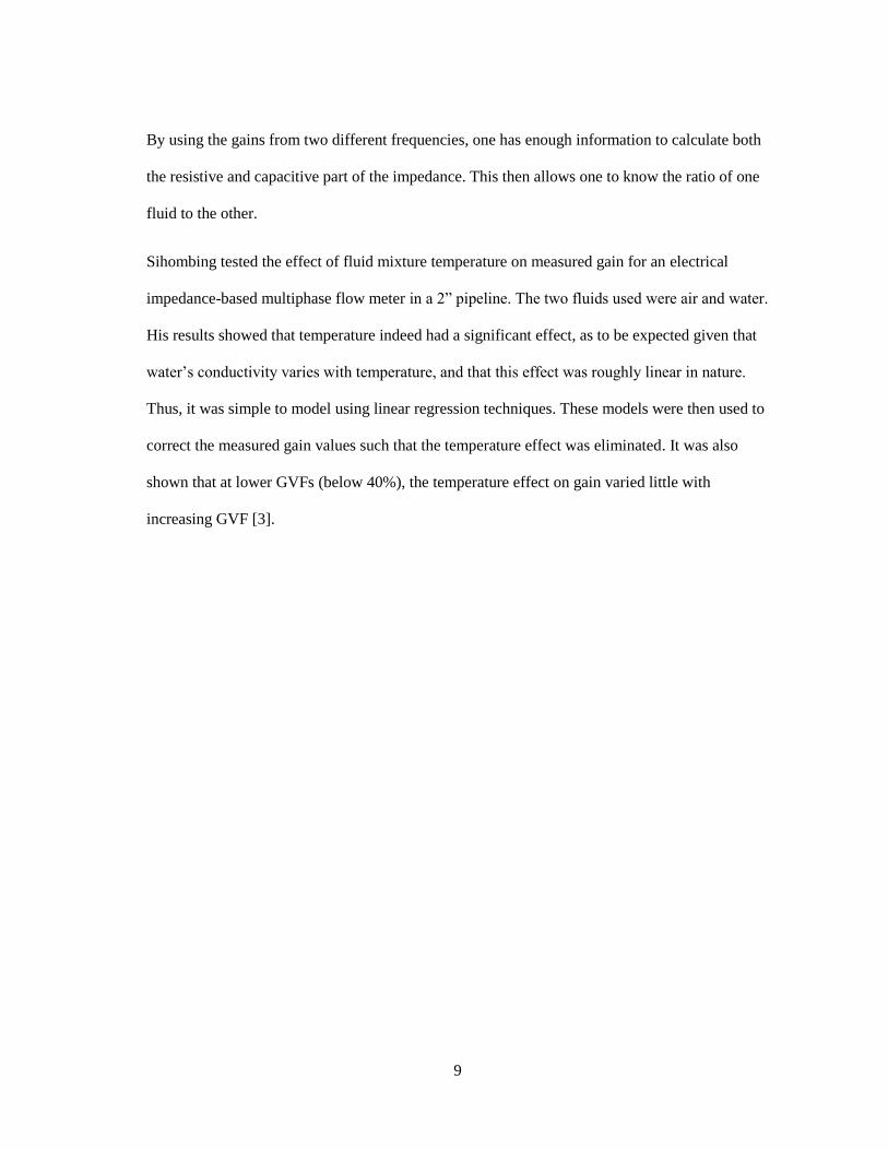
Sihombing tested the effect of fluid mixture temperature on measured gain for an electrical
impedance-based multiphase flow meter in a 2” pipeline. The two fluids used were air and water.
His results showed that temperature indeed had a significant effect, as to be expected given that
water’s conductivity varies with temperature, and that this effect was roughly linear in nature.
Thus, it was simple to model using linear regression techniques. These models were then used to
correct the measured gain values such that the temperature effect was eliminated. It was also
shown that at lower GVFs (below 40%), the temperature effect on gain varied little with
increasing GVF [3].

10
3. OBJECTIVES
The following objectives were pursued in this experiment:
Design and construct a low-cost electrical impedance-based MPFM for use in larger
diameter (6”) pipes.
Determine what variables affect the signal gain of the MPFM.
Determine the ability of the MPFM to measure both the % GVF and total flow rate
through a pipe.
Determine whether the electrical impedance-based design can function accurately in a 6”
pipeline.
Determine whether the electrical impedance-based design can function at higher flow
rates and pressures than previous experiments.
Develop calibration equations to convert measured data into flow rate measurements for
each component of a two-phase flow.

11
4. EXPERIMENTAL FACILITIES AND METHODS
This section will describe the design and construction of the MPFM as well as the test facility
used to evaluate its performance.
4.1 MPFM Conceptual Design
Figure 4 and Figure 5 display SolidWorks renderings of the MPFM used in the study. It follows
a wafer-style design, and is made to fit in line with NPS 6” schedule 40 piping. The MPFM is
compressed between two 600# flanges with both ends sealed using spiral-wound gaskets. It
consists of both an alumina-enclosed electrode assembly and a slotted orifice plate meter, both
contained in a stainless steel housing.
Figure 4. Exploded view of MPFM assembly
12
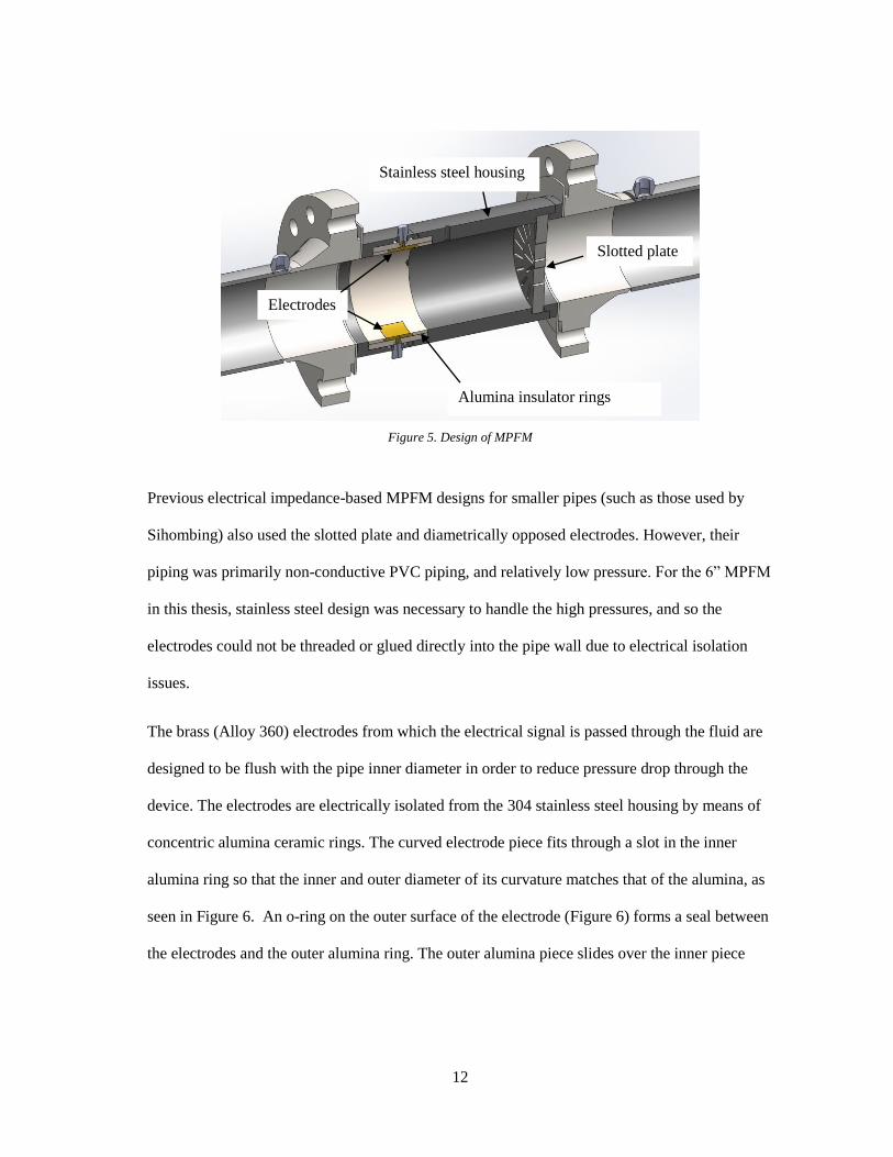
Figure 5. Design of MPFM
Previous electrical impedance-based MPFM designs for smaller pipes (such as those used by
Sihombing) also used the slotted plate and diametrically opposed electrodes. However, their
piping was primarily non-conductive PVC piping, and relatively low pressure. For the 6” MPFM
in this thesis, stainless steel design was necessary to handle the high pressures, and so the
electrodes could not be threaded or glued directly into the pipe wall due to electrical isolation
issues.
The brass (Alloy 360) electrodes from which the electrical signal is passed through the fluid are
designed to be flush with the pipe inner diameter in order to reduce pressure drop through the
device. The electrodes are electrically isolated from the 304 stainless steel housing by means of
concentric alumina ceramic rings. The curved electrode piece fits through a slot in the inner
alumina ring so that the inner and outer diameter of its curvature matches that of the alumina, as
seen in Figure 6. An o-ring on the outer surface of the electrode (Figure 6) forms a seal between
the electrodes and the outer alumina ring. The outer alumina piece slides over the inner piece
Electrodes
Slotted plate
Alumina insulator rings
Stainless steel housing

13
after the o-rings are in place, completing the electrode assembly. The outer alumina piece has
holes through which electrical wire can pass to be bonded to the electrode.
Figure 6. Axial cross-sectional view of MPFM for electrode sealing and wiring detail
The housing is made of three interlocking stainless steel pieces. Between these fit both the
slotted orifice plate and the electrode assembly alumina ring. An o-ring face seal is used to seal
between the two pieces that surround the electrode assembly, as seen in Figure 7. O-ring grooves
are also present in order to form face seals on both sides of the slotted plate, as seen in Figure 8.
Between the stainless steel shell and the electrode assembly, o-ring gland seals were used to
prevent leakage through the electrode wiring holes, as seen in Figure 7.
Stainless Steel Housing
Outer alumina ring
Inner alumina ring
Brass electrode
Cord grip
Face seal between
electrode and alumina

14
Figure 7. Radial cross-sectional view of MPFM to show housing o-ring details
Figure 8. Radial cross sectional view to show slotted plate sealing detail and pressure taps
The electrodes are located approximately 1.5 diameters downstream of the slotted plate (9
inches). This ensures the most homogeneous flow at the electrodes, according to Annamalai
Face seal between
housing pieces Gland seal between
housing and alumina
Slotted plate
Downstream
pressure tap Upstream pressure
tap with weldolet
Face seals between
housing and slotted
plate

15
[15]. The electrical wiring is bonded to the electrodes using a high conductivity silver epoxy and
held in place using cable grips threaded into the housing.
The slotted plate was designed with a beta ratio β of 0.496. This ratio is very close to the ideal
two phase performance ratio for a slotted plate of approximately 0.5 [13]. The slot sizes and
arrangement relative to the overall pipe diameter are identical to those used by Sihombing with
2” pipe, and so it is a direct scale-up of these 2” slotted plates [3]. This simplifies comparison of
the performance. The number of concentric rings of slots and number of slots per ring was
selected by previous researchers for its ability to produce a roughly parabolic velocity profile
coming out of the plate, improving the distance needed for a fully developed profile [22].It was
manufactured using electric discharge manufacturing.
A pressure tap is located in the housing after the slotted plate to allow the measurement of the
pressure at that location, while the upstream pressure tap is actually located in the upstream
piping as seen in Figure 8. The upstream tap is used to measure the absolute pressure, the
upstream temperature, and the high pressure end of a differential pressure measurement.
4.2 Measurement and Data Acquisition
An Omega PX429-500GI pressure transducer was used to measure the absolute pressure in the
MPFM upstream pressure tap. This transducer has an operating range of 0-500 psig and an
accuracy of ±0.4 psig. An Omega TQSS-18U-6 T-type thermocouple was used in the upstream
tap to measure temperature. It has a measurement accuracy of ±0.6 °F, and can withstand
temperatures up to 220 °C. A Rosemount 3051CD3A22A1A differential pressure transducer was
used to measure the pressure difference across the slotted plate, with the high pressure line using
the upstream tap, and the low pressure line using the downstream tap. It has an operating range
of 36 psig, with ±0.05 psig accuracy, and generates a 4-20 mA signal.

16
Figure 9. Rosemount pressure transducers used to measure slotted plate and venturi differential pressures
Figure 10. Omega pressure transducer

17
Figure 11. Omega thermocouple
GVF was measured using the electrical impedance method proven by Pirouzpanah (2014) and
Sihombing (2015) [20][3]. A Picoscope 5442B oscilloscope/function generator device was used
to generate the various frequencies to be passed through the fluid as well as measure the signal
conditioner output. Its arbitrary waveform generator (AWG) can generate signals at 200 MS/s
and it has a 500 MS/s sampling rate with 12-bit resolution. Using two channels in this
experiment divided the sampling rate so that it has a maximum of 250 MS/s per channel. The
twelve frequencies used in the experiment were: 200 kHz, 600 kHz, 1 MHz, 1.28 MHz, 2.37
MHz, 3.46 MHz, 4.55 MHz, 5.64 MHz, 6.73 MHz, 7.82 MHz, 8.91 MHz, and 10 MHz. These
twelve frequencies were added together to produce one combined signal that was uploaded to the
Picoscope as the AWG’s reference waveform. The combined signal output was passed through
the fluid mixture and signal conditioning circuit. Both the direct output from the Picoscope and
the output from the fluid mixture and signal conditioner circuit were monitored using the
Picoscope’s input channels, as seen in Figure 12.

18
Figure 12. Signal generation and capture schematic.
LabVIEW programs were used in the control room to operate the test rig remotely. Figure 13
shows the program used to monitor the pump’s performance and the various pressures,
temperatures, and flow rates throughout the test loop. It also used PID control algorithms to
operate the loop’s control valves in order to maintain the user’s desired pump inlet pressure,
water flow rate, and GVF of the fluid mixture. Pressure transducer signals were read using NI
9205 voltage measurement modules in an NI cRIO-9074 chassis. Thermocouples were
connected to an NI 9213 thermocouple measurement module in the same chassis.

19
Figure 13. Pump control and fluid flow monitoring program
Figure 14 shows the program used to monitor the pump’s vibration performance. In this
experiment, this was used solely to ensure that the pump shaft’s orbit did not indicate any
impending mechanical failure.

20
Figure 14. Pump vibration monitoring program
Figure 15 shows the program used to control the Picoscope and collect the MPFM signal data. It
is set up to be able to operate all input channels at one time, but only two channels were
activated during the experiment. The user pushes the “Take Data” button to copy the Picoscope’s
current memory buffer to the computer for further data processing. The program automatically
names the collected data files using the current flow conditions in the loop.

21
Figure 15. Picoscope control and MPFM data capture program
Figure 16 shows the circuit to be used to determine the frequency response of the test flows. The
flow itself is modeled as a resistor and capacitor in parallel. The signal conditioning part of the
circuit is an analog low-pass filter amplifier with a cut-off frequency of 15.9 MHz to filter out
unwanted noise above the max generated signal frequency of 10 MHz. The op amp used in the
circuit was a Texas Instruments LM7171 op amp with max current output of 100 mA and a
supply voltage requirement of ±15V.
Figure 16. Circuit diagram for MPFM
Flow
Rf 220 Ω
Cf 10 pF

22
Figure 17. Filter circuit with 3 different amplifier circuits
Ordinarily, the Picoscope interfaces with a computer using USB. However, because the
Picoscope was located inside the test cell (in order to reduce signal noise due to wire length), a
USB-to-ethernet adapter was used to reach the computer in the control room. The equipment
used was an IOGear GUWIP204 as seen in Figure 18. This device acts as a router that the
computer can access to communicate across its multiple USB ports.
Figure 18. Inside of MPFM circuitry box with filter circuit, USB-to-ethernet converter/extender, and Picoscope signal
generator/digital oscilloscope

23
4.3 Closed-loop Test Facility
Figure 19 is a process and instrumentation diagram of the flow loop used during testing, while
Figure 20 is a SolidWorks rendering of the loop. It has three main fluid flow paths driven by a
single pump: a water inlet line, an air inlet line, and a mixed outlet line. It is a closed loop
system, with water and air lines converging at the pump inlet to create the air/water mixture that
flows through the pump and then through the outlet line to a large stainless steel tank. The
stainless steel tank acts as both a reservoir and a separator for the air and water. It can handle
pressures up to 450 psi and has a total volume of 1760 gallons. Water is pulled from the bottom
of the tank through the water inlet line, while air is pulled from the top of the tank through the air
inlet line. The test loop is pressurized by injecting compressed air into the top of the tank until it
reaches the desired pressure.
Figure 19. Process and instrumentation diagram of flow loop.

24
Figure 20. SolidWorks rendering of closed loop test facility (Kirkland [21])
Control valves (Figure 21) are located on the air and water inlet lines as well as at the pump
outlet to control the water, air, and overall flow rates through the pump. They are operated
remotely using a LabVIEW program, and follow a PID control algorithm. Turbine flow meters
are also located on the air and water lines to measure the flow rates of each component (Figure
22). The water turbine meter is a Turbines, Inc. WM0600X6, and has an accuracy of ±1% over
the range 250-2500 gpm. The air turbine meter is an Omega FTB-938 with an accuracy of ±1%
and a range of 60-970 gpm. The flow rates obtained are used to calculate the GVF of the fluid
flow.

25
Figure 21. Control valve on outlet line
Figure 22. Turbine meter used to measure water flow in the inlet line
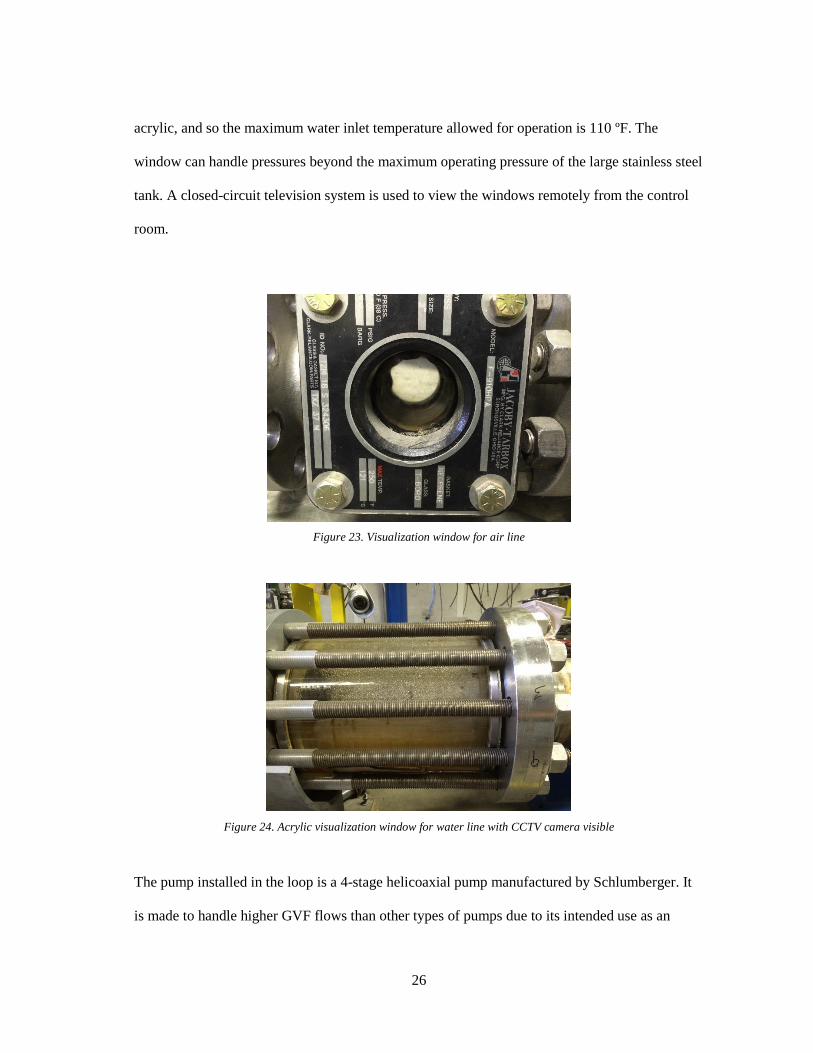
It is important to ensure that air is not in the water line, nor water in the air line. Either case will
negatively impact the flow rate measurements, and could even damage the turbine meters. In
order to monitor the air and water inlet lines for this kind of contamination, visualization
windows are installed inline, as seen in Figure 23 and Figure 24. The air window is made of
glass, and can handle pressures up to 720 psig and temperatures up to 250 ºF. These constraints
are far less restrictive than other system components. The water window, however, is made of
26
acrylic, and so the maximum water inlet temperature allowed for operation is 110 ºF. The
window can handle pressures beyond the maximum operating pressure of the large stainless steel
tank. A closed-circuit television system is used to view the windows remotely from the control
room.
Figure 23. Visualization window for air line
Figure 24. Acrylic visualization window for water line with CCTV camera visible
The pump installed in the loop is a 4-stage helicoaxial pump manufactured by Schlumberger. It
is made to handle higher GVF flows than other types of pumps due to its intended use as an

27
electrical submersible pump in deep-sea oil extraction. It is driven by a 250 HP electric motor
controlled using a variable frequency drive (VFD) at speeds of up to 3600 rpm. The pump is
mounted under a test stand made to withstand both the thrust generated by the pump and the
weight of the electric motor that is mounted above. This setup can be seen in Figure 25.
Figure 25. Inside of closed loop test facility. Pump is beneath motor stand (right). Control valves and inlet/exit piping
are at left.
The top bearing of the pump is cooled using an auxiliary oil loop, seen in Figure 26, that uses a
heat exchanger to cool the oil. Room temperature water is used as the other process fluid in the

28
heat exchanger. The bottom bearing is located at the pump inlet, and so is cooled by the
incoming air and water.
Figure 26. Bearing oil heat exchanger loop
A mechanical seal at the very top of the pump requires a constant flow of water to operate
correctly. Thus, a seal flush pump is used to pump water from the bottom of the outside large
tank through the seal and back into the tank. Figure 27 shows the seal flush pump skid.
From bearing To bearing

29
Figure 27. Seal flush pump skid (disconnected during disassembly)
In order to prevent overheating of the air and water in the large tank, an additional heat
exchanger loop takes water out of the bottom of the tank and runs it through a filter and large
heat exchanger, seen in Figure 28. Temperature in the water inlet line must be kept below 110 ºF
because of the clear acrylic pipe section. Figure 29 is a schematic of the heat exchanger loop.
Figure 28. Heat exchanger fan and pump (left) and large stainless steel tank for water/air reservoir (right).

30
Figure 29. Heat exchanger loop
The MPFM assembly was placed after the outlet valve of the test loop’s main pump. The piping
was designed so that the entire MPFM would be at least 5 diameters downstream of the outlet
valve to minimize flow effects associated with the valve.
A venturi flow tube was placed just downstream of the MPFM to provide additional flow rate
measurement validation. It was manufactured within a pipe spool so that it could be easily
swapped for a section of plain pipe if desired. Figure 30 shows this design concept. It has a beta
ratio of 0.5, and three pressure taps: one at the inlet before the contraction, one in the contracted
portion, and one at the outlet following the expansion. A Rosemount 3051CD3A22A1A
differential pressure transducer identical to that used with the slotted plate was used to measure
the differential pressure between the venturi inlet and its contracted portion. Omega PX429-
500GI pressure transducers were also used to measure gage pressure at the venturi inlet and
outlet pressure taps. Another Omega TQSS-18U-6 T-type thermocouple was installed at the
To tank
From tank

31
venturi outlet pressure tap. Given that venturi tubes have very high pressure recovery (and, thus,
low losses) this outlet temperature reading should be the same as the temperature between the
electrodes and was used as such.
Figure 30. Drawing of venturi built inside pipe spool
4.4 Assembly
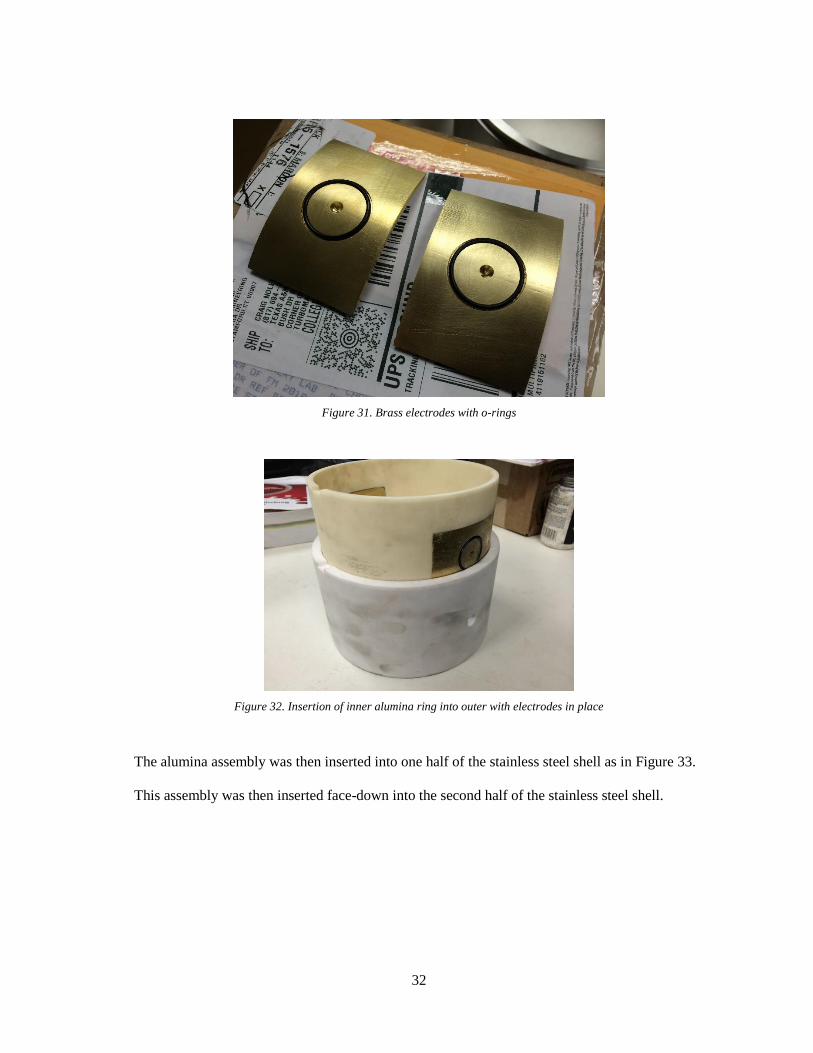
Figures 31-36 help illustrate the assembly and installation of the MPFM as manufactured. Figure
31 shows the brass electrodes with their o-rings in-groove. These were inserted into their mating
slots in the inner alumina ring, which was then inserted into the outer alumina ring as shown by
Figure 32. O-rings were placed in their grooves in the stainless steel shell pieces.
32
Figure 31. Brass electrodes with o-rings
Figure 32. Insertion of inner alumina ring into outer with electrodes in place
The alumina assembly was then inserted into one half of the stainless steel shell as in Figure 33.
This assembly was then inserted face-down into the second half of the stainless steel shell.

33
Figure 33. Alumina inserted into outer shell.
The slotted plate was placed between the final two shell pieces—completing the wafer assembly.
Figure 34 illustrates the slotted plate’s geometry.
Figure 34. Slotted plate in assembled MPFM shell
Electrical wire was attached with high-conductivity silver epoxy to the electrodes and supported
by cord grips to prevent breaking. The completed MPFM wafer was then inserted between two

34
6” 600 lb flanges and tightened to the corresponding torque. Figure 35 shows the MPFM being
fitted between the two flanges—one of which belonged to the venturi tube. Figure 36 shows the
assembly in place in the closed loop facility with all electrical connections, thermocouples, and
pressure transducers installed.
Figure 35. MPFM being installed between two pipe flanges. Electrical connections installed on sides.

35
Figure 36. Finished assembly with all thermocouples, pressure transducers, and electrical connections intact.
4.5 Testing Plan
Once everything was installed, the pump was operated at various flow rates, pressures, and
GVF’s. Both the generated signal and the MPFM output signal were recorded for each flow
condition in order to determine the MPFM’s response to these varying conditions. The test
matrix tested (as achievable by the pump) was:
Pressure: 40, 100, 185, and 280 psi
GVF: 0, 10, 20, 30, 40%
Flow rate: 305, 395, 485, 570, 654, 737, 820 gpm
Each test session consisted of pressurizing the loop to the desired pressure and operating at that
pressure for each combination of GVF and flow rate. Typically, only one pressure could be
tested per day.

36
Temperatures were recorded for each condition to be used to treat the gain according to the
technique developed by Sihombing [3]. In order to collect gain versus temperature data for the
temperature correction method, separate tests were run for each GVF where flow rate, pressure,
and GVF were held constant as the fluid temperature increased from room temperature to
approximately 100 °F.
Slotted plate and venturi differential pressures were recorded for all conditions tested in order to
calibrate their respective devices.

37
5. RESULTS AND DISCUSSION
This section will discuss the test results as well as develop calibration equations for the MPFM.
5.1 Flow Conditions Tested
At higher flow rates, it was not possible to achieve the higher GVF flows due to limitations of
the pump. Additionally, it was proven difficult to achieve the lowest GVF flows for the lowest
flow rates tested. Table 1 illustrates the flow conditions that were possible during testing. These
limitations were consistent for each pressure tested, except for the 40 psi data, where 10% GVF
and 395 gpm were also not possible.
Table 1. Flow conditions possible during testing
Flow Rates (gpm)
% GVF 305 395 485 570 654 737 820
0
10 X
20
30 X
40 X X
Not possible X Possible
5.2 GVF Measurements
The signal gain was calculated for each flow condition and frequency by dividing the signal
amplitude coming from the MPFM electrodes by the signal amplitude generated by the
Picoscope, as seen in Equation 4.
𝐺𝑎𝑖𝑛 =𝑀𝑃𝐹𝑀 𝐴𝑚𝑝𝑙𝑖𝑡𝑢𝑑𝑒
𝐺𝑒𝑛𝑒𝑟𝑎𝑡𝑒𝑑 𝐴𝑚𝑝𝑙𝑖𝑡𝑢𝑑𝑒
(4)
Plotting the signal gains versus frequency for each GVF shows that, for most frequencies,
increasing GVF tends to decrease the gain, as seen in Figure 37. Because of its large difference
in gain between 0 and 40% GVF, 7.82 MHz was chosen as the primary frequency to be used for

38
subsequent analysis. This large gain difference at 7.82 MHz was consistent for all pressures and
flow rates tested.
Figure 37. Gain vs. frequency (185 psi, 570 gpm) with 95% error bars shown
Because previous studies have shown a significant temperature effect on the gain, it was
necessary to correct each gain based on its corresponding temperature [3]. This was
accomplished, first, by plotting the gain versus temperature for each frequency while GVF,

39
pressure, and flow rate remained constant. A 2nd order polynomial regression was applied to the
data as seen in Figure 38.
Figure 38. Gain vs. temperature (7.82 MHz, 0% GVF, 50 psig, 537 gpm)
Using the regression equation, it was possible to calculate the correction factor to be subtracted
from each gain so that each gain has effectively the same temperature. Equations 5-8 detail this
process, where Gainref and Tref are a reference gain and temperature relative to which the
correction factor Δ𝐺𝑎𝑖𝑛 is calculated. The constants a, b, and c are the polynomial coefficients of
the regression equation, and c0 is a constant made to simplify the final gain correction factor
equation.
𝐶𝑜𝑟𝑟𝑒𝑐𝑡𝑖𝑜𝑛 𝐹𝑎𝑐𝑡𝑜𝑟 = 𝐺𝑎𝑖𝑛 − 𝐺𝑎𝑖𝑛𝑟𝑒𝑓 = Δ𝐺𝑎𝑖𝑛 (5)
Δ𝐺𝑎𝑖𝑛 = (𝑎𝑇2 + 𝑏𝑇 + 𝑐) − (𝑎𝑇𝑟𝑒𝑓2 + 𝑏𝑇𝑟𝑒𝑓 + 𝑐) (6)

40
Δ𝐺𝑎𝑖𝑛 = 𝑎𝑇2 + 𝑏𝑇 + 𝑐0, where 𝑐0 = −(𝑎𝑇𝑟𝑒𝑓2 + 𝑏𝑇𝑟𝑒𝑓) (7)
𝐶𝑜𝑟𝑟𝑒𝑐𝑡𝑒𝑑 𝐺𝑎𝑖𝑛 = 𝐺𝑎𝑖𝑛 − Δ𝐺𝑎𝑖𝑛 (8)
The temperature effect’s slope did not appear to vary much with GVF, pressure, or flow rate, as
seen in Figure 39. The only exception appears in the 30% data, which shows a decreased slope.
Because the goal of the experiment is to estimate the GVF of the fluid mixture, however, the
GVF cannot be used during the temperature correction or else the conclusions would fall prey to
circular reasoning. Additionally, the results of the work done by Sihombing (2015) showed that
at low GVFs, the temperature effect did not vary much with changing GVF. Therefore, a single
regression equation per frequency was used to correct the gain data.
Figure 39. Gain vs. temperature for different GVFs
Table 2 displays the calculated correction factor equations for each frequency.

41
Table 2. Regression equations for temperature correction
Frequency Gain Correction Coefficients
(𝚫𝑮𝒂𝒊𝒏 = 𝒂𝑻𝟐 + 𝒃𝑻 + 𝒄𝟎)
a b c
0.2 MHz -6.78E-06 0.001415 -0.06914
0.6 MHz -2.23E-05 0.005708 -0.30951
1.0 MHz -3.87E-05 0.00956 -0.51043
1.28 MHz -6.06E-05 0.012605 -0.61428
2.37 MHz -2.29E-05 0.005589 -0.29647
3.46 MHz -1.72E-05 0.006538 -0.40559
4.55 MHz -1.69E-06 0.00207 -0.15117
5.64 MHz 7.42E-06 1.84E-05 -0.04659
6.73 MHz 3.47E-05 -0.00394 0.096318
7.82 MHz 9.72E-05 -0.01343 0.455644
8.91 MHz 6.87E-05 -0.01177 0.499897
10.0 MHz -2.65E-05 0.004535 -0.19256
The gain for each GVF was plotted versus its corresponding fluid static pressure in order to
visualize how pressure affected the gain. This was done for each flow rate tested. As can be seen

42
in Figure 40, there was no clear visual trend with pressure within the uncertainties of the data.
This was true for each flow rate tested.
Figure 40. Gain vs. pressure for different GVFs (654 gpm)
The effect of water flow rate on gain was also investigated. Figure 41 shows gain plotted versus
flow rate for different GVFs at 120 psig. It appears that water flow rate does have an effect on
the gain: it decreases as the flow rate increases. However, this effect is only visible with air in
the fluid, and appears to grow stronger with higher GVF. The fact that the water flow rate effect
is not consistent across all GVFs and, in fact, appears to be dependent on GVF means that a
simple correction like that used to correct for temperature is not possible. This flow rate effect

43
was not seen in the study conducted by Sihombing, and is thus likely to be a result of up-scaling
the design. [3]
Figure 41. Gain vs. water flow rate for different GVFs (120 psig)
Although the position of the electrodes downstream of the slotted plate was chosen to be in the
most homogeneously mixed region, the flow condition data was overlain on a flow regime map
in order to help determine whether some sort of transition between flow regimes could explain
the flow rate trend. Figure 42 shows this overlay. It is clearly seen that each flow condition was
well inside the elongated bubbly flow region. So, even without a slotted plate mixing the flow,
the flow should not undergo a regime transition.

44
Figure 42. Flow regime map with experimental data overlayed (Mandhane, 1974 [7])
One possible reason for the flow rate and GVF trend is poor mixing from the slotted plate. When
the slotted plate was designed, it was directly scaled up from a smaller version, and so the slot
size is the same relative to the overall diameter of the pipe. These larger slots would likely not
homogenize the flow to the same scale seen with the smaller slots. This would explain the larger
variation in gains seen at higher GVFs, as there is more air passing through the plate needing to
be mixed. The decrease in gain with flow rate could be due to the difference in electrical flow
path geometry when larger bubbles are present.
Because visual inspection of graphs did not give many clear insights into whether the
experiment’s three remaining independent variables (pressure, flow rate, and GVF) had an effect
on the gain, a 3-way analysis of variance (ANOVA) was performed on the data. However, the
test matrix was imbalanced (i.e. some flow conditions could not be tested due to limitations of
the pump), and so typical ANOVA techniques could not be applied. The number of levels of

45
each individual variable was reduced to that seen in Table 3 in order to have a balanced matrix.
In theory, if the ANOVA results show significance for a variable or interaction between
variables in the reduced table, it should also indicate significance in the full table. This is due to
ANOVA taking into account the levels and degrees of freedom of the test matrix.
Table 3. Reduced test matrix for balanced ANOVA
Variable Conditions # of Levels
Flow Rate 305, 570, 737 3
Pressure 50, 300 2
GVF 0, 20, 30 3
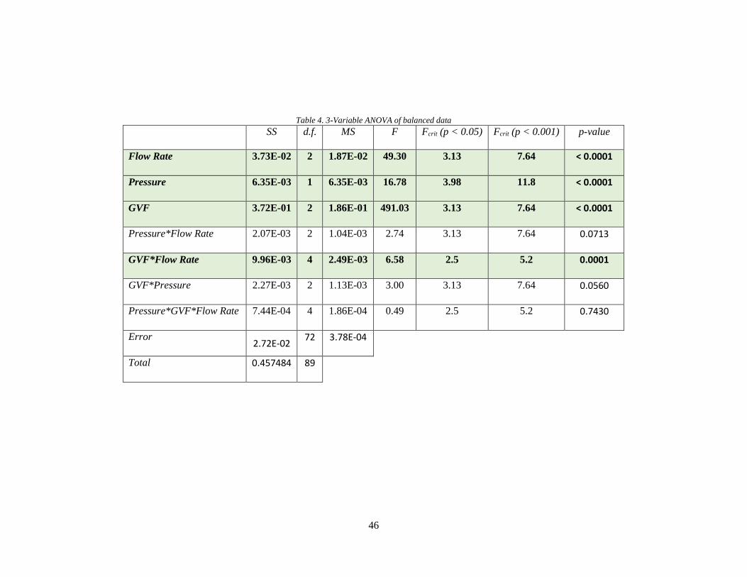
Table 4 shows the results of the ANOVA. Main effects and interactions that passed the test for
significance are highlighted. The results showed that with greater than 99.99% confidence, flow
rate, pressure, and GVF affected the gain. Additionally, the interaction between GVF and flow
rate is also highly significant.
46
Table 4. 3-Variable ANOVA of balanced data
SS d.f. MS F Fcrit (p < 0.05) Fcrit (p < 0.001) p-value
Flow Rate 3.73E-02 2 1.87E-02 49.30 3.13 7.64 < 0.0001
Pressure 6.35E-03 1 6.35E-03 16.78 3.98 11.8 < 0.0001
GVF 3.72E-01 2 1.86E-01 491.03 3.13 7.64 < 0.0001
Pressure*Flow Rate 2.07E-03 2 1.04E-03 2.74 3.13 7.64 0.0713
GVF*Flow Rate 9.96E-03 4 2.49E-03 6.58 2.5 5.2 0.0001
GVF*Pressure 2.27E-03 2 1.13E-03 3.00 3.13 7.64 0.0560
Pressure*GVF*Flow Rate 7.44E-04 4 1.86E-04 0.49 2.5 5.2 0.7430
Error 2.72E-02
72 3.78E-04
Total 0.457484 89

47
Thus, the results of the ANOVA confirmed that flow rate and GVF were affecting the gain, as
well as the inference that one was influencing the effect of the other. Additionally, it showed that
pressure was affecting the gain despite it not being visually obvious.
Given the ANOVA results, a multi-variable linear quadratic regression with three independent
and one dependent variable as well as interaction effects was applied to the data in order to find
an equation to accurately predict GVF. The fluid static pressure, total mass flow rate, and signal
gain were treated as the independent variables, while GVF was the dependent. Equation 6 is the
regression result, where 𝐺𝑉𝐹𝑝 is the equation-predicted GVF, P is the fluid static pressure, is
the total mass flow rate, and 𝐺𝑎𝑖𝑛 is the signal gain. Equation 9 has an r-square value of 0.963,
and predicts the GVF within ±5.3% of its actual value with 95% confidence. Table 5 displays the
coefficients for the equation.
𝐺𝑉𝐹𝑝 = 𝐴 + 𝐵(𝑃) + 𝐶(𝐺𝑎𝑖𝑛) + 𝐷() + 𝐸(𝑃 ∗ 𝐺𝑎𝑖𝑛) + 𝐹(𝑃 ∗ ) + 𝐺(𝐺𝑎𝑖𝑛 ∗ ) + 𝐻(𝑃2)
+ 𝐼(𝐺𝑎𝑖𝑛2) + 𝐽(2)
(9)

48
Table 5. Coefficients table for Equation 6
Coefficient Value
A 7.60E+01
B 3.84E-03
C 1.43E+02
D -2.25E+00
E 4.20E-02
F -1.54E-04
G 2.53E+00
H -9.73E-05
I -2.73E+02
J 1.08E-03
Investigation of the relative contribution of each term in Equation 9 to the GVF prediction
resulted in Figure 43. The contribution was calculated first by totaling the absolute value of each
term in the equation, then by dividing each term by this absolute value total to obtain a
percentage. Figure 43 shows that the major contributors to the calculation of GVF appear to be
the constant term, gain and its squared term, flow rate, and the flow rate/GVF interaction. So, if

49
one desired to produce a simpler equation with fewer terms for calculations in the field, it is
likely that one could perform a regression using only these terms and achieve similar accuracy.
Figure 43. Graph of percentage contribution of each term (named by its coefficient) in Equation 9 to the GVF
estimate.
5.3 Flow Rate Measurements
In order to have a fully functional MPFM, it is also necessary to calibrate the flow rate
measurement devices. Equation 10 is the standard equation used for slotted plate orifice meters,
where is the total mass flow rate, 𝐶𝐷 is the coefficient of discharge of the plate, 𝐴𝑓 is the flow
area of the meter, 𝜌 is the fluid density, Δ𝑝 is the pressure difference across the plate, and 𝛽 is
the area ratio defined by Equation 11, where 𝐴𝑡 is the cross-sectional area of the pipe upstream
Constant Term
Gain2
GVF*Flow Rate Flow Rate
Gain

50
of the plate. Solving Equation 10 for 𝐶𝐷 gives Equation 12, which was used to calculate the
coefficient of discharge of the slotted plate for each flow condition tested.
=𝐶𝐷
√1 − 𝛽4𝐴𝑓√2𝜌Δ𝑝
(10)
𝛽 = √𝐴𝑓
𝐴𝑡
(11)
𝐶𝐷 =√1 − 𝛽4
𝐴𝑓√2𝜌Δ𝑝
(12)
Figure 44 shows the calculated values of CD plotted versus the density and mass flow rate of the
flow. Most of the 𝐶𝐷 values hover between 0.75 and 0.85 in Figure 44, but there is another
cluster of 𝐶𝐷 values that instead float between 0.6 and 0.7. Plotting the data with pressure on one
independent axis rather than mass flow rate showed that most of these points belonged to the 50
psi static pressure data set (Figure 45).

51
Figure 44. Slotted plate CD vs. mass flow rate and density
Figure 45. Slotted plate CD vs. pressure and density

52
Plotting the data versus total mass flow rate showed a decreasing trend in the slotted plate’s
discharge coefficient with increasing total mass flow rate, as seen in Figure 46, Figure 47, Figure
48, and Figure 49. Any trend associated with changing GVF is difficult to discern except in the
300 psig data of Figure 49, where increasing GVF appears to lower the discharge coefficient.
The literature has shown that a slotted plate’s discharge coefficient should decrease with GVF,
so the trend seen at 300 psig is consistent with the literature [4].
Figure 46. Slotted plate CD vs. mass flow rate and density at 50 psig

53
Figure 47. Slotted plate CD vs. mass flow rate and density at 120 psig
Figure 48. Slotted plate CD vs. mass flow rate and density at 200 psig

54
Figure 49. Slotted plate CD vs. mass flow rate and density at 300 psig
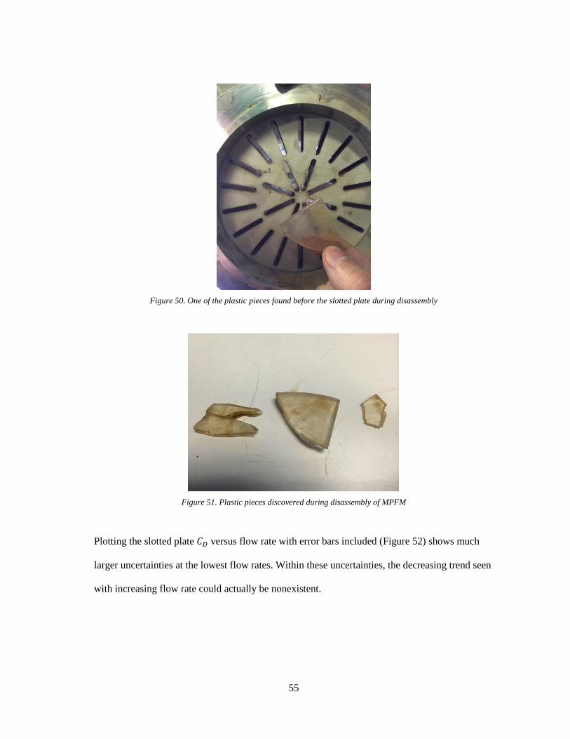
Upon removal of the MPFM from the test loop, several large pieces of plastic were found in the
piping upstream of the slotted plate, as seen in Figure 50 and Figure 51. These were most likely
from the previous experiment of another student that shares the same outlet piping. During this
other experiment, the acrylic pump being used failed and destroyed its own impeller. It is
possible that one or more of these plastic pieces became lodged in or blocked a portion of the
slotted plate during part of the 50 psi testing. This additional blockage would reduce the
coefficient of discharge of the plate, and thus is a possible explanation for the discrepancy.
55
Figure 50. One of the plastic pieces found before the slotted plate during disassembly
Figure 51. Plastic pieces discovered during disassembly of MPFM
Plotting the slotted plate 𝐶𝐷 versus flow rate with error bars included (Figure 52) shows much
larger uncertainties at the lowest flow rates. Within these uncertainties, the decreasing trend seen
with increasing flow rate could actually be nonexistent.

56
Figure 52. Slotted plate CD vs. total mass flow rate with error bars
The uncertainties seen at lower flow rates appear to be mostly due to fluctuations in the flow
rate. As the flow rate approaches the lower limit of the pump, these fluctuations increase
dramatically. Figure 53 shows the standard deviation in flow rate for each data point versus their
flow rate. Based on this correlation, it seems that for this test setup, predicting the exact flow rate
is more difficult at lower flow rates.

57
Figure 53. Standard deviation in mass flow rate vs. mass flow rate
Calibration of the Venturi tube flow meter was performed similarly to that of the slotted plate, as
the equations are very similar. Equations 13-15 apply to the venturi, where 𝐶𝐷,𝑣 is the coefficient
of discharge for the venturi, 𝛽𝑣 is its area ratio, 𝐴2 is the cross-sectional area of the constricted
portion of the venturi, and all other variables are identical to those of the slotted plate.
=𝐶𝐷,𝑣
√1 − 𝛽4𝐴2√2𝜌Δ𝑝
(13)
𝛽𝑣 = √𝐴2
𝐴1
(14)
𝐶𝐷,𝑣 =√1 − 𝛽4
𝐴2√2𝜌Δ𝑝
(15)

58
Figure 54 shows 𝐶𝐷,𝑣 plotted versus the mass flow rate and density. It can be seen that the
calculated 𝐶𝐷,𝑣 stays fairly close to a value of 1, as expected for a venturi.
Figure 54. Venturi CD vs. mass flow rate and density
Plotting the venturi’s CD versus total mass flow rate did not show the same consistent decrease in
CD with increasing mass flow rate seen for the slotted plate except at the higher pressures of 200
and 300 psi, as seen in Figure 55, Figure 56, Figure 57, and Figure 58. Again, any trend
associated with GVF is difficult to discern.

59
Figure 55. Venturi CD vs. mass flow rate and density at 50 psig
Figure 56. Venturi CD vs. mass flow rate and density at 120 psig

60
Figure 57. Venturi CD vs. mass flow rate and density at 200 psig
Figure 58. Venturi CD vs. mass flow rate and density at 300 psig

61
Plotting the venturi CD versus mass flow rate with error bars included showed the same trend as
with the slotted plate: increased uncertainty for lower flow rates. Again, this is likely due to the
fluctuations in flow rate seen at lower flow rates. Similarly, this implies greater difficulty in
predicting flow rate at lower flow rates even for the venturi.
Figure 59. Venturi CD vs. total mass flow rate
Selecting a single CD for each flow measurement device to re-calculate the flow rates using their
respective equations showed measurement accuracies displayed in Table 6. The CD’s were
selected by averaging the calculated CD’s for the slotted plate, and by trial-and-error iterations
for the venturi. The slotted plate showed a large measurement uncertainty of ±19.1% with 95%
confidence while looking at all data points. If one removes the anomalous CD data points from
the analysis, however, the uncertainty is improved to ±8.80%. This is still about twice the
uncertainty of a typical slotted orifice plate meter. The venturi showed a measurement

62
uncertainty of ±4.53%, which is not optimal for a venturi, but is still certainly within its range.
Due to the higher accuracy of the venturi meter (and confounded nature of the slotted plate data),
it is the primary device used in determining the overall measurement accuracy of the MPFM.
Table 6. Flow measurement device accuracies
Flow measurement device CD used
Uncertainty
(95% confidence)
Slotted plate 0.7535 ±19.1%
Slotted plate (anomalous points removed) 0.7854 ±8.80%
Venturi 0.9983 ±4.53%
5.4 Combined GVF and Flow Rate Measurements
The flow rate prediction accuracy reported in Table 6, however, is only valid when the density of
the fluid is already known. This would likely not be the case in a situation where this MPFM is
needed, as the MPFM provides the GVF, and therefore density, information. Since flow rate was
shown to have a significant effect on the GVF predictions of the MPFM, both GVF and flow rate
are interdependent. In other words, to know one accurately, one must know the other.
This trap can be avoided, however, using an iterative prediction method as follows:
1. An initial GVF prediction is obtained by assuming an arbitrary flow rate (in this case,
the mean flow rate condition tested) in Equation 9
2. Flow rate is calculated using the initial GVF prediction in Equation 13.
3. The flow rate obtained from Equation 13 is used in Equation 9 to obtain a better GVF
prediction.

63
4. This improved GVF is used to better predict the flow rate using Equation 13.
5. Steps 3 and 4 are repeated until the percent change in GVF or flow rate from each
iteration to the next is minimal.
For this analysis, the above method was allowed to continue until the change in predicted flow
rate from iteration to iteration was less than 0.1%. This resulted in flow rate measurements with
an uncertainty of ±6.14% of the actual value with 95% confidence. GVF measurements showed
uncertainty of ±5.85% GVF. These results are similar to those seen by Sihombing (2015),
showing that the MPFM concept appears valid even for NPS 6” piping and the more extreme
pressures and flow rates tested.
The MPFM design was also relatively inexpensive to produce: the entire prototype including
DAQ equipment and the venturi tube flow meter cost less than $50,000. In large scale
production, this cost would be reduced significantly.

64
6. CONCLUSIONS AND RECOMMENDATIONS
The testing and evaluation of the electrical impedance-based MPFM for large diameter pipe
described in this thesis showed that multiple variables and mixture properties affected the
meter’s readings: signal frequency, temperature, pressure, flow rate, and mixture GVF. The
signal gains corresponding to the 7.82 MHz frequency showed the strongest difference across the
GVFs tested, making 7.82 MHz the primary frequency used for analysis. It was possible to use
regression techniques to eliminate the temperature effect for each frequency and GVF tested.
The temperature correction factor equations were found not to vary much with GVF, and so the
correction equation for 0% GVF could be used.
Analysis of variance techniques were applied to the data and confirmed that pressure, total mass
flow rate, GVF, and the interaction between flow rate and GVF all had a statistically significant
effect on the MPFM’s gain. Flow rate and pressure effects had not been seen with 2” electrical
impedance-based MPFMs of similar design. Based on the ANOVA results, a multi-variable
regression was performed on the data to obtain a calibration equation for the MPFM. This
equation was capable of predicting the GVF of the fluid mixture within ±5.3% GVF with 95%
confidence given knowledge of the flow rate.
Calculations of the discharge coefficient were carried out for both the slotted plate and venturi
tube flow meters. The slotted plate data had anomalies that could possibly be explained by large
pieces of plastic found upstream that could have blocked flow through the plate during
operation. Ignoring the anomalous data, however, the slotted plate predicted the total flow rate of
the fluid mixture with an uncertainty of ±8.8%. The venturi had much more consistent data, and
could predict total flow rate with an uncertainty of ±4.53%.

65
However, these flow rate prediction accuracies are based on knowing the density (or GVF) of the
fluid mixture. So, in order for the MPFM to function accurately, an iterative method was applied
to estimate both GVF and total flow rate. This method resulted in flow rate prediction with an
uncertainty of ±6.14%, and GVF prediction uncertainty of ±5.85% GVF.
Based on these results, it appears that the MPFM design described in this report has the potential
to be a viable flow measurement device for air-water flows in pipes as large as 6”, with water
flow rates as high as 820 gpm and pressures upward of 350 psig. In addition, it is relatively low
cost—the prototype being constructed for less than $50,000. In order to improve the
measurement accuracy of the MPFM in future testing, the following recommendations are made:
Reduce slot size while maintaining 𝛽 ratio of slotted plate. This could improve mixing of
the two fluids, as mixture homogeneity does not necessarily remain the same as slot size
is increased [14].
Increase output voltage of signal generation device. For smaller pipe diameters (and
especially those of pipes made of polymers), the ±2V from the Picoscope was sufficient.
With a larger diameter, however, there is more room for variation in flow patterns, and
so a stronger signal could overpower more signal noise.
Increase the signal measurement buffer size. This would help reduce random error in the
data.
While the MPFM conceptual design sufficed for this experiment, several areas of improvement
were identified throughout the testing experience:
Eliminating the alumina rings in favor of alumina inserts of some kind would reduce the
risk of failure due to having the ceramic in tension. While precautions were taken to
minimize the amount of tension to be seen in the current design and the rings remained

66
intact during testing, the ring design does have inherent risk due to putting the ceramic in
tension. The alumina rings were also considerably expensive, and so reducing the size
and manufacturing difficulty of the insulator parts would greatly reduce cost.
Manufacturing the brass electrodes in a way that allows wire to be soldered to the
electrode prior to installation in the device would be preferred over the current
configuration which required attachment through the small access hole in the housing.

67
REFERENCES
[1] Falcone, G. (2001). Multiphase Flow Metering: Current Trends and Future Developments.
Proceedings of the 2001 Society of Petroleum Engineers Annual Technical Conference, New
Orleans, LA.
[2] Da Silva, M. J. (2008). Impedance sensors for fast multiphase flow measurement and
imaging (Doctoral dissertation). Technische Universtaat Dresden, Dresden, Germany.
[3] Sihombing, D. (2015) Temperature Effect in Multiphase Flow Meter Using Slotted Orifice
Plate (Master’s thesis). Texas A&M University, College Station, Texas.
[4] Morrison, G. L., Pirouzpanah, S., Cevik, M., & Patil, A. (2013, July 7-11). Evaluation of a
close coupled slotted orifice, electrical impedance, and swirl flow meters for multiphase flow.
Proceedings of the ASME 2013 Fluids Engineering Division Summer Meeting, Incline Village,
NV. Retrieved June 11, 2015, from http://proceedings.asmedigitalcollection.asme.org
[5] Andreussi, P., Di Donfransesco, A. D., & Messi, M. (1988). An impedance method for the
measurement of liquid hold-up in two-phase flow. International Journal Multiphase Flow, 14(6),
777-785.
[6] Corneliussen, S., Couput, J. P., Dahl, E., Dykesteen, E., Froysa, K. E., Malde, E., &
Tunheim, H. (2005). Handbook of the multiphase flow metering (Rev. 2). The Norwegian
Society for Oil and Gas Measurement and The Norwegian Society of Chartered Technical and
Scientific Professionals. Retrieved November 6, 2014, from http://www.nfogm.no
[7] Mandhane, J. M., Gregory, G. A., & Aziz, K. (1974). A flow pattern map for gas-liquid flow
in horizontal pipes. International Journal Multiphase Flow, 1, 537-553.

68
[8] Coleman, J. W., & Garimella, S. (1999). Characterization of two-phase flow patterns in small
diameter round and rectangular tubes. International of Heat and Mass Transfer, 42, 2869-2881.
[9] Bratland, O. (2013). Pipe Flow 2: Multi-phase flow assurance. Retrieved June 25, 2015, from
http://www.drbratland.com
[10] Orifice, Nozzle, and Venturi Flow Rate Meters. The Engineering ToolBox. Accessed June
30, 2015. http://www.engineeringtoolbox.com/orifice-nozzle-venturi-d_590.html
[11] Morrison, G. L., Hall K. R., Holste, J. C., Macek, M. L., Ihfe, L. M., DeOtte, R. E., Jr., &
Terracina, D. P. (1994). Comparison of Orifice and Slotted Plate Flowmeters. Flow
Measurement and Instrumentation, 5(2), 71-74.
[12]Macek, M. L. (1993). A Slotted Orifice Plate Used as a Flow Measurement Device (Master’s
thesis). Texas A&M University, College Station, TX.
[13] Morrison, G. L., Terracina, D. P., & Brewer, C. (2001). Response of a slotted orifice flow
meter to an air/water mixture. Flow Measurement and Instrumentation, 12, 175-180.
[14] Sparks, S. A. (2004). Two phase mixing comparison, oil contamination comparison, and
manufacturing accuracy effect on calibration of slotted orifice flow meters (Master’s thesis).
Texas A&M University, College Station, TX.
[15] Annamalai, G. (2014). Characterization of flow homogeneity downstream of a slotted plate
in a two-phase flow using electrical resistance tomography (Master’s thesis). Texas A&M
University, College Station, TX.
[16] Liptak, B. (2003). Instrument Engineers’ Handbook: Process Measurement and Analysis,
Fourth Edition.. Boca Raton, Florida. CRC Press.

69
[17] Hasan, Abbas (2012). Theoretical and Experimental Study of Bubbly Gas-water Two Phase
Flows through a universal venturi tube. International Journal of Information Science and
Education, 2(1), 43-58.
[18] Thorn, R., Johansen, G. A., & Hjertaker, B. T. (2013). Three-phase flow measurement in
the petroleum industry. Measurement Science and Technology, 24(1), 1-17. doi:10.1088/0957-
0233/24/1/012003
[19] Fossa, M. (1998). Design and performance of a conductance probe for measuring the liquid
fraction in two-phase gas-liquid flows. Flow Measurement and Instrumentation, 9, 103-109.
[20] Pirouzpanah, S. (2014). Study of hysteresis and emulsion properties in watercut
measurement using high speed multi-frequency impedance sensor. Flow Measurement and
Instrumentation, 40, 1-8.
[21] Kirkland, K. (2012). Design and fabrication of a vertical pump multiphase flow loop
(Master’s thesis). Texas A&M University, College Station, TX.
[22] Ihfe, L. M. (1994). Development of the slotted orifice flow conditioner (Master’s thesis).
Texas A&M University, College Station, TX.
[23] Baker, R. C. (2000). Flow Measurement Handbook: Industrial Designs, Operating
Principles, and Applications. Cambridge, UK: Cambridge University Press.
[24] Geng, Y., Zheng, J., & Shi, T. (2006). Study on the metering characteristics of a slotted
orifice for wet gas flow. Flow Measurement and Instrumentation, 17, 123-128.
[25] Husain, Z. (1995). Theoretical Uncertainty of Orifice Flow Measurement. Daniel Flow
Products, Inc. Accessed July 8, 2015. http://docslide.us/documents/theoretical-uncertainty-of-
orifice-flow-measurement-172kb.html
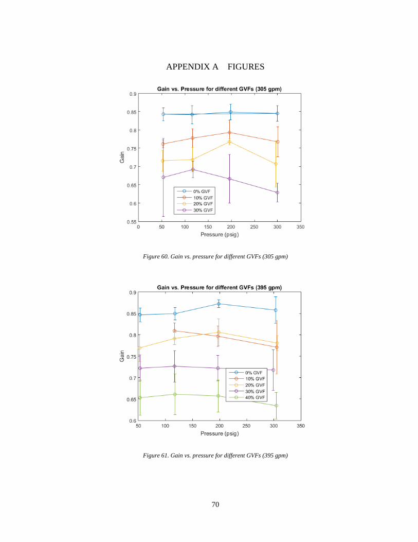
70
APPENDIX A FIGURES
Figure 60. Gain vs. pressure for different GVFs (305 gpm)
Figure 61. Gain vs. pressure for different GVFs (395 gpm)

71
Figure 62. Gain vs. pressure for different GVFs (485 gpm)
Figure 63. Gain vs. pressure for different GVFs (570 gpm)

72
Figure 64. Gain vs. pressure for different GVFs (654 gpm)
Figure 65. Gain vs. pressure for different GVFs (737 gpm)

73
Figure 66. Gain vs. pressure for different GVFs (820 gpm)
Figure 67. Gain vs. water flow rate for different GVFs (50 psig)

74
Figure 68. Gain vs. water flow rate for different GVFs (120 psig)
Figure 69. Gain vs. water flow rate for different GVFs (200 psig)

75
Figure 70. Gain vs. water flow rate for different GVFs (320 psig)
Figure 71. Gain vs. temperature (0.2 MHz)

76
Figure 72. Gain vs. temperature (0.6 MHz)
Figure 73. Gain vs. temperature (1.0 MHz)

77
Figure 74. Gain vs. temperature (1.28 MHz)
Figure 75. Gain vs. temperature (2.37 MHz)
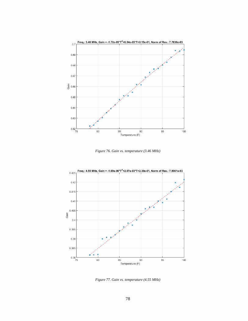
78
Figure 76. Gain vs. temperature (3.46 MHz)
Figure 77. Gain vs. temperature (4.55 MHz)

79
Figure 78. Gain vs. temperature (5.64 MHz)
Figure 79. Gain vs. temperature (6.73 MHz)

80
Figure 80. Gain vs. temperature (7.82 MHz)
Figure 81. Gain vs. temperature (8.91 MHz)

81
Figure 82. Gain vs. temperature (10 MHz)

82
Figure 83. Gain vs. total mass flow rate and % GVF (0.2 MHz)
Figure 84. Gain vs. total mass flow rate and % GVF (0.6 MHz)

83
Figure 85. Gain vs. total mass flow rate and % GVF (1.0 MHz)
Figure 86. Gain vs. total mass flow rate and % GVF (1.28 MHz)

84
Figure 87. Gain vs. total mass flow rate and % GVF (2.37 MHz)
Figure 88. Gain vs. total mass flow rate and % GVF (3.46 MHz)

85
Figure 89. Gain vs. total mass flow rate and % GVF (4.55 MHz)
Figure 90. Gain vs. total mass flow rate and % GVF (5.64 MHz)
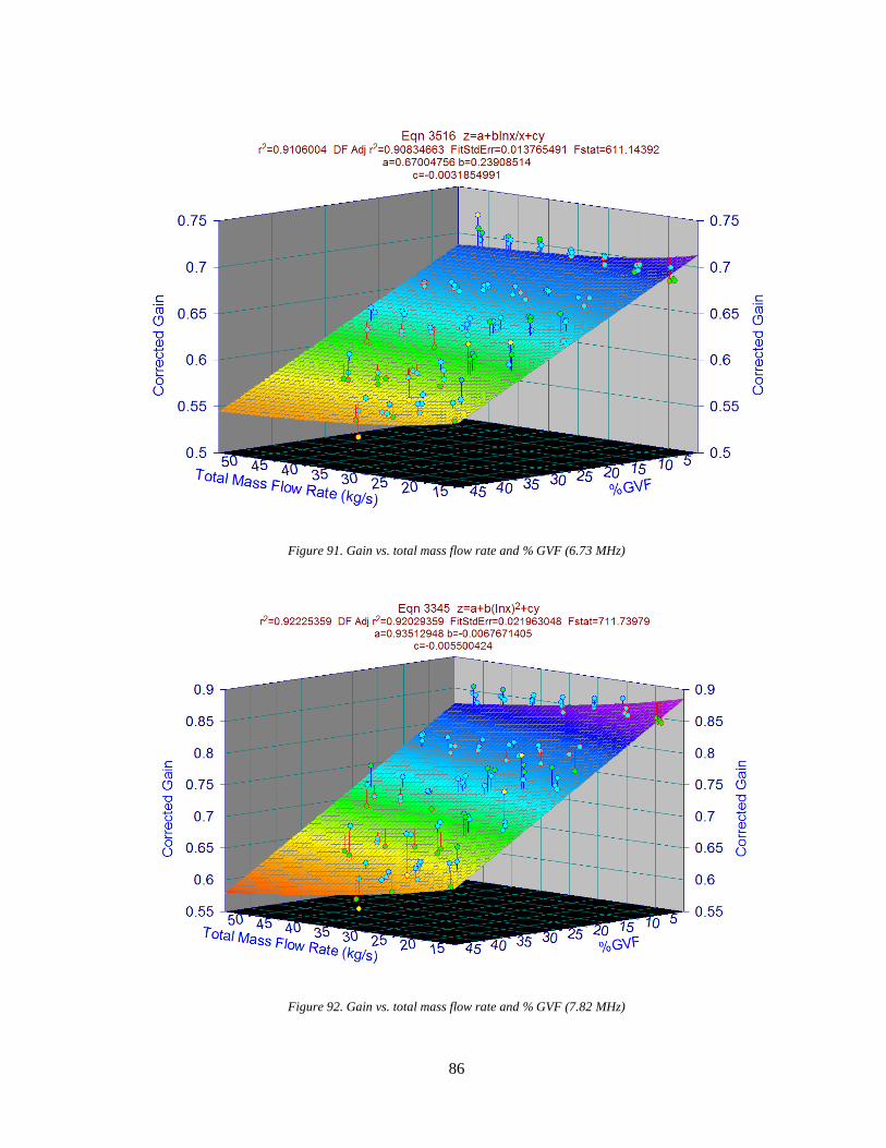
86
Figure 91. Gain vs. total mass flow rate and % GVF (6.73 MHz)
Figure 92. Gain vs. total mass flow rate and % GVF (7.82 MHz)

87
Figure 93. Gain vs. total mass flow rate and % GVF (8.91 MHz)
Figure 94. Gain vs. total mass flow rate and % GVF (10 MHz)

88
Figure 95. Slotted plate CD vs. density and mass flow rate at 50 psig
Figure 96. Slotted plate CD vs. mass flow rate and density at 50 psig

89
Figure 97. Venturi CD vs. density and mass flow rate at 50 psig
Figure 98. Venturi CD vs. mass flow rate and density at 50 psig

90
Figure 99. Venturi CD vs. mass flow rate and density at 120 psig
Figure 100. Slotted plate CD vs. density and mass flow rate at 120 psig

91
Figure 101. Slotted plate CD vs. mass flow rate and density at 120 psig
Figure 102. Venturi CD vs. density and mass flow rate at 120 psig

92
Figure 103. Slotted plate CD vs. density and mass flow rate at 200 psig
Figure 104. Slotted plate CD vs. mass flow rate and density at 200 psig

93
Figure 105. Venturi CD vs. density and mass flow rate at 200 psig
Figure 106. Venturi CD vs. mass flow rate and density at 200 psig

94
Figure 107. Slotted plate CD vs. density and mass flow rate at 300 psig
Figure 108. Slotted plate CD vs. mass flow rate and density at 300 psig

95
Figure 109. Venturi CD vs. density and mass flow rate at 300 psig
Figure 110. Venturi CD vs. mass flow rate and density at 300 psig
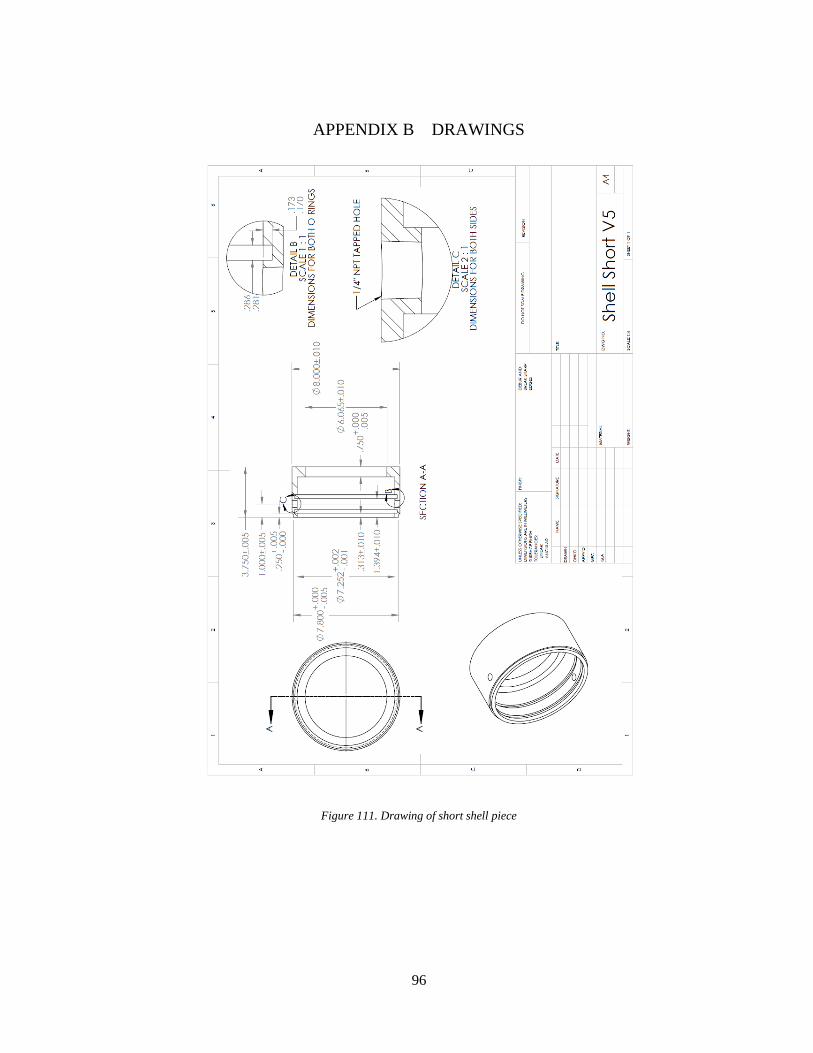
96
APPENDIX B DRAWINGS
Figure 111. Drawing of short shell piece

97
Figure 112. Drawing of long shell piece

98
Figure 113. Drawing of slotted plate

99
Figure 114. Drawing of shell cap piece

100
Figure 115. Drawing of pipe assembly with MPFM

101
Figure 116. Drawing of long pipe spool

102
Figure 117. Drawing of short pipe spool

103
Figure 118. Drawing of inner alumina ring

104
Figure 119. Drawing of outer alumina ring

105
Figure 120. Drawing of brass electrode