design and simulation of a dc electric … · i design and simulation of a dc electric vehicle...
TRANSCRIPT

i
DESIGN AND SIMULATION OF A DC ELECTRIC VEHICLE CHARGING STATION INTERCONNECTED WITH A MVDC NETWORK
by
Adam Richard Sparacino
B.S. in Electrical Engineering, University of Pittsburgh, 2011
Submitted to the Graduate Faculty of
Swanson School of Engineering in partial fulfillment
of the requirements for the degree of
Master of Science
University of Pittsburgh
2012

ii
UNIVERSITY OF PITTSBURGH
SWANSON SCHOOL OF ENGINEERING
This thesis was presented
by
Adam Richard Sparacino
It was defended on
November 6, 2012
and approved by
Gregory F. Reed, PhD, Associate Professor, Electrical and Computer Engineering Department
George Kusic, PhD, Associate Professor, Electrical and Computer Engineering
Zhi-Hong Mao, PhD, Associate Professor, Electrical and Computer Engineering
Thesis Advisor: Gregory F. Reed, PhD, Associate Professor, Electrical and Computer
Engineering Department

iii
Copyright © by Adam Richard Sparacino
2012

iv
DESIGN AND SIMULATION OF A DC ELECTRIC VEHICLE CHARGING STATION INTERCONNECTED WITH A MVDC NETWORK
Adam Sparacino, M.S.
University of Pittsburgh, 2012
Due to a rapidly aging electric transmission and distribution infrastructure, an increased demand
for energy, an increased awareness of climate change and greenhouse gas pollution, and an
increased cost of fuel there is a need to produce and deliver energy more efficiently. This thesis
attempts to provide a solution to these constraints through advancements in DC power
architectures.
Medium Voltage Direct Current (MVDC) infrastructure serves as a platform for the
interconnection of renewable electric power generation, including wind and solar. Abundant
loads such as industrial facilities, data centers, commercial office buildings, industrial parks, and
electric vehicle charging stations (EVCS) can also be powered using MVDC technology. MVDC
networks are expected to improve efficiency, through reductions in power electronic conversion
steps and by serving as an additional layer between the transmission and distribution level
voltage for which generation sources and loads could directly interface with smaller rated power
conversion equipment.
This thesis provides an introduction to battery energy storage system technology, and
primarily investigates an EVCS powered via a MVDC bus. A bidirectional DC-DC converter
with appropriate controls serves as the interface between the EVCS and the MVDC bus. Two
scenarios are investigated for testing and comparing EVCS operation: 1) EVCS power supplied
by the interconnected MVDC model and 2) EVCS power supplied by an equivalent voltage
source. The ability of the battery charger (synchronous buck converter) to isolate faults in next

v
generation DC power systems is explored. Each of the investigated components is modeled and
simulated utilizing the PSCAD simulation environment then analytically validated.
vi
TABLE OF CONTENTS
ACKNOWLEDGEMENTS ....................................................................................................... 13
1.0 INTRODUCTION ........................................................................................................ 1
1.1 MEDIUM VOLTAGE DC NETWORK ............................................................ 2
1.2 ELECTRIC VEHICLE CHARGING STATION............................................. 3
1.3 PROBLEM STATEMENT AND MOTIVATION ........................................... 4
1.4 ORGANIZATION OF DOCUMENT ................................................................ 5
2.0 BATTERY ENERGY STORAGE SYSTEMS .......................................................... 7
2.1 SURVEY OF BATTERY ENERGY STORAGE SYSTEM TECHNOLOGIES ............................................................................................... 9
2.2 BATTERY MODELING .................................................................................. 13
2.2.1 Electrochemical Models ................................................................................ 14
2.2.2 Equivalent Circuit Models ............................................................................ 16
3.0 SYSTEM LAYOUT AND DESIGN ......................................................................... 18
3.1 MVDC NETWORK........................................................................................... 19
3.1.1 Wind Power Generation Model Development ............................................ 19
3.1.2 Three Level NPC Converter ......................................................................... 21
3.1.3 Industrial Facility .......................................................................................... 23
3.2 EV CHARGING STATION ............................................................................. 24
3.2.1 Design Criteria for the EV Charging Station ............................................. 25

vii
3.2.2 Bidirectional DC-DC Converter ................................................................... 27
3.2.3 Synchronous Buck Converter....................................................................... 36
3.2.4 Electric Vehicle Linear Battery Model ........................................................ 38
3.2.5 Photovoltaic Array and Boost Converter .................................................... 41
4.0 PSCAD COMPONENT VALIDATION .................................................................. 45
4.1 MVDC SYSTEM COMPONENT VALIDATION ......................................... 45
4.1.1 5 MW PMSG Wind Turbine ........................................................................ 45
4.1.2 Three Level NPC Converter ......................................................................... 46
4.1.3 10 kW Induction Machine ............................................................................ 47
4.2 EVCS SYSTEM COMPONENT VALIDATION ........................................... 48
4.2.1 Bidirectional DC-DC Converter ................................................................... 49
4.2.2 Synchronous Buck Converter....................................................................... 55
4.2.3 Linear Battery Model .................................................................................... 58
4.2.4 Photovoltaic Array ........................................................................................ 60
5.0 SYSTEM ANALYSIS, OPERATION, AND RESULTS ........................................ 63
5.1 RESPONSE OF EVCS WITH AND WITHOUT MVDC GRID MODEL INTERCONNECTION ..................................................................................... 64
5.2 SYNCHRONOUS BUCK CONVERTER TRANSIENT PROPAGATION 69
5.3 CCM / DCM BUCK MODE OPERATION OF BIDIRECTIONAL DC-DC CONVERTER .................................................................................................... 75
6.0 CONCLUSIONS AND FUTURE WORK ............................................................... 80
BIBLIOGRAPHY ....................................................................................................................... 83

viii
LIST OF TABLES
Table 1. Comparison of Energy Storage Technologies [9-12] ..................................................... 10
Table 2. Wind Turbine & PMSG Parameters [4] ......................................................................... 21
Table 3. Logic Table for Switching States of the Three Level Neutral Point Clamp Inverter [4, 43] .................................................................................................................................. 22
Table 4. Induction Machine Equivalent Circuit Parameters [43] ................................................. 24
Table 5. Operating Parameters Bidirectional DC-DC Converter ................................................. 36
Table 6. Operating Parameters Linear Battery Model ................................................................. 41
Table 7. Kyocera Solar KC125G Module [61] ............................................................................ 43
Table 8. Operating Regime for testing of the EVCS During Various Modes of Operation ........ 65
Table 9. Operating Regime for EVCS Fault Test ......................................................................... 71

ix
LIST OF FIGURES
Figure 1-1. Medium Voltage DC (MVDC) System Architecture [4] ............................................. 3
Figure 2-1. Worldwide installed energy storage capacity [9] ......................................................... 8
Figure 2-2. Power rating versus discharge time at rated power for various energy storage technologies [9] ........................................................................................................... 9
Figure 2-3. NaS battery electrochemical reaction [19] ................................................................. 12
Figure 2-4. Ideal battery equivalent circuit model ........................................................................ 16
Figure 2-5. Linear battery equivalent circuit model ..................................................................... 17
Figure 2-6. Thevenin battery equivalent circuit model ................................................................. 17
Figure 3-1. PSCAD MVDC Interconnected Model ...................................................................... 18
Figure 3-2. Three Level NPC Converter [4, 43] ........................................................................... 22
Figure 3-3. Three-Level Neutral Point Clamped Converter Single Phase Switching States [4, 43] ................................................................................................................................... 23
Figure 3-4. Per-Phase Equivalent Circuit of an Induction Motor [44] ......................................... 24
Figure 3-5. Electric Vehicle Charging Station One Line Diagram ............................................... 26
Figure 3-6. Electric Vehicle Charging Station with Solar Generation [52] .................................. 26
Figure 3-7. Bidirectional DC-DC Converter ................................................................................ 28
Figure 3-8. Bidirectional DC-DC Converter Boost Mode Operating Waveforms ....................... 29
Figure 3-9. Boost Mode Converter Current Paths for Operating States ....................................... 30

x
Figure 3-10. Bidirectional DC-DC Converter Buck Mode Operating Waveforms ...................... 31
Figure 3-11. Buck Mode Converter Current Paths for Operating States ...................................... 32
Figure 3-12. Controller for Bidirectional DC-DC Converter Buck Mode Voltage Regulation ... 35
Figure 3-13. Bidirectional DC-DC Converter with Pre-charge Circuit and Damping Circuit ..... 36
Figure 3-14. Synchronous Buck Converter .................................................................................. 37
Figure 3-15. Constant Power Feedback Controller....................................................................... 37
Figure 3-16. Key Operating Waveforms of Synchronous Buck Converter .................................. 37
Figure 3-17. Charging Profile for a Lithium-Ion Phosphate Battery [54] .................................... 39
Figure 3-18. Electric Vehicle Linear Battery Model .................................................................... 40
Figure 3-19. PV Array equivalent circuit model [4] ..................................................................... 42
Figure 3-20. Comparison of theoretical and simulated V-I curves for a single PV module [4] ... 42
Figure 3-21. Incremental Conductance Maximum Power Point Tracking Algorithm [63]d ....... 44
Figure 4-1. Mechanical and Electrical Output Power of Permanent Machine Synchronous Generator.................................................................................................................. 46
Figure 4-2. Line-to-Line Input Voltage of Three Level NPC Rectifier ........................................ 47
Figure 4-3. Instantaneous Power Absorbed by Each Induction Machine ..................................... 48
Figure 4-4. EVCS PSCAD Implementation ................................................................................. 49
Figure 4-5. Bidirectional DC-DC Converter PSCAD Implementation ........................................ 50
Figure 4-6. Bidirectional DC-DC Converter Buck Mode Constant Voltage Controller .............. 50
Figure 4-7. Buck Mode Gating Signals ........................................................................................ 51
Figure 4-8. Primary Side Voltage (EP) and Secondary Side Voltage (ES) ................................... 52
Figure 4-9. Choke Inductor Current (iL) ....................................................................................... 53
Figure 4-10. Leakage Inductance Current (iLK) ............................................................................ 54
Figure 4-11. High Voltage Side Input Current (iHV) ..................................................................... 55

xi
Figure 4-12. Synchronous Buck Converter PSCAD Implementation .......................................... 56
Figure 4-13. Synchronous Buck Converter Controller and Gating Signal Driver ........................ 56
Figure 4-14. Synchronous Buck Converter Output Voltage (VLV) ............................................... 57
Figure 4-15. Synchronous Buck Converter Output Current (ILV) ................................................. 57
Figure 4-16. PSCAD Implementation of Linear Battery Model................................................... 58
Figure 4-17. PSCAD Calculation of SOC .................................................................................... 58
Figure 4-18. EV Battery 2 Pulse Charge Voltage and Current ..................................................... 59
Figure 4-19. Example Li-Ion Battery Pulse Charge [64] .............................................................. 60
Figure 4-20. PV Array and Boost Converter PSCAD Implementation ........................................ 60
Figure 4-21. PSCAD Implementation of Incremental Conductance Algorithm........................... 61
Figure 4-22. PV Array Output Power Test System ...................................................................... 62
Figure 5-1. Regulated MVDC Bus Voltage .................................................................................. 67
Figure 5-2. Regulated LVDC Bus Voltage ................................................................................... 67
Figure 5-3. EVCS Component Absorbed and Received Power ................................................... 68
Figure 5-4. Bidirectional DC-DC Converter LVDC Bus Output Current (ILV) ............................ 69
Figure 5-5. Line to Line Fault Applied to Terminal of EV During Charging .............................. 70
Figure 5-6. EVCS Component Absorbed and Received Power During Fault Operation ............. 72
Figure 5-7. LVDC Bus Voltage and Synchronous Buck Converter Output Voltage During Fault Operation ................................................................................................................... 72
Figure 5-8. Synchronous Buck Converter Output Voltage During Fault Operation .................... 73
Figure 5-9. Synchronous Buck Converter Output Power During Fault Operation....................... 74
Figure 5-10. Fault Current and Contributing Sources .................................................................. 75
Figure 5-11. Buck Converter CCM Inductor Current Ripple [58] ............................................... 76
Figure 5-12. Buck Converter DCM Inductor Current Ripple [58] ............................................... 77

xii
Figure 5-13. Choke Inductor Current (IL) at Various fS ................................................................ 78
Figure 5-14. Transformer Primary Voltage (EP) at Various fS ..................................................... 79

xiii
ACKNOWLEDGEMENTS
Primarily, I would like to my parents who have always encouraged me to question and pursue a
greater understanding of the world around me and have been influential in helping me achieve
success both personally and academically. They have always made it clear that they believe in
me and pushed me to be the best I could be. I would also like to give a special thanks to my
siblings Courtney and Matthew who have always been there for me and in general being my best
friends in the world without them I wouldn’t be the person I am today.
I would like to thank my thesis advisor Dr. Reed for giving me the opportunity to pursue
an advanced degree and for being there to provide career and life advice. Dr. Kusic for being an
excellent source of knowledge and for the fun times we’ve had together. Dr. Mao for his constant
encouragement to be the best you can be. Dr. McDermott who joined the department in the last
semester of my Masters education has provided guidance as well as been there to listen and help
formulate the ideas that have gone into the creation of this document.
I would like to thank my graduate student peers. These are the people who make it
possible and enjoyable to come to work every day. These people have helped me immeasurably
over the last year and a half and are all great friends. Listed in no particular order they are
Brandon Grainger, Robert Kerestes, Emanuel Taylor, Matthew Korytowski, Rusty Scioscia,
Hashim Al Hassan, Hussain Bassi, Patrick Lewis, Ansel Barchowsky, Alvaro Cardoza, Benoit
De Courreges, Jean-Marc Coulomb, Raghav Khanna, Raymond Kovacs and Azime Can.

1
1.0 INTRODUCTION
Due to a rapidly aging electric transmission and distribution infrastructure, an increased demand
for energy and an increased awareness of climate change and greenhouse gas pollution, there is a
need to produce and deliver energy more efficiently. Current industry and government solutions
point to the development of a smart grid. The electric power energy research for grid
infrastructure (EPERGI) team at the University of Pittsburgh defines smart grid as “The
implementation of various enabling power technologies that allow real-time interoperability
between end-users and energy producers, in order to enhance efficiency in utilization decision-
making based on energy resource availability and economics.” d Based upon investigation of
representative approaches of various independent entities, utilities, and manufacturers, gaps
within existing smart grid enabling technology were identified. These gaps included: improved
control of transmission and distribution, energy storage, renewable integration, information and
incentives for both the end-user and the utility [1]. This thesis attempts to establish how next
generation DC power systems, and power conversion devices can be used to provide enhanced
control, utilization, and efficiency as a key enabling technology of the smart grid. Two main
topics in particular are investigated and simulated using PSCAD, a medium voltage direct
current (MVDC) network, and a common direct current (DC) bus electric vehicle charging
station (EVCS).

2
1.1 MEDIUM VOLTAGE DC NETWORK
Over the past five decades high voltage direct current (HVDC) technology has proven its merit
as a reliable and efficient method of delivering bulk power over long distance / under water, and
linking asynchronous power networks [2]. At the medium voltage levels, DC power systems
have received usage within naval power systems [3]. Beyond these limited applications, DC
systems have not found widespread use. The medium voltage direct current (MVDC) concept is
conceived as a collection platform which will provide an additional layer of infrastructure
between transmission and distribution to help integrate renewable generation (photovoltaic,
wind), energy storage, and various end-use loads (industrial facilities, data centers). A general
overview of the proposed MVDC architecture is shown in Figure 1-1. It should be noted that the
MVDC system is not a simple scaling of voltage level from HVDC and has distinct applications.
MVDC systems will help to reduce the number of conversion stages necessary for integrating the
lower voltage output of renewable generation resources to the electric grid operating at a much
higher voltage whereas HVDC is used for interconnection of asynchronous grids and long
distance transmission of power.

3
DC
AC
DC
DC
DC
AC
DC
AC
Non-Synchronous Generation (Wind)
Distribution Level
Storage
DC
DC
Photovoltaic Generation
DC
DC
Fuel Cells
Electric Vehicle
AC
DC
DC
DC
Distribution DC Load Circuits
Sensitive Load
Electronic and AC Loads
Future DC Industrial Facility
DC
DC
AC Transmission Supply
Future DC Data
Centers
DC
DC
Existing AC Infrastructure
DC
DC
MVDC
HVDC System
Future HVDC Intertie
AC
DC
DC
DC
Motor
Variable Frequency
Drives
Figure 1-1. Medium Voltage DC (MVDC) System Architecture [4]
1.2 ELECTRIC VEHICLE CHARGING STATION
Presently, the vast majority of energy consumption by the transportation sector comes from
petroleum [5]. Vehicles with unconventional fuel systems (flex-fuel, diesel, hybrid-electric)
constituted 15 percent of new vehicles sales in 2009 [5]. While electric vehicles make up a small
percentage of vehicles sold, consumers are comfortable with buying vehicles containing
alternative fuel systems. Auto manufacturers large (General Motors and Nissan) and small (Tesla

4
Motors) are beginning to manufacture and produce full electric vehicles. The United States
government predicts that over one million electric vehicles will be on the road in the United
States by 2015 [6]. These predictions of increased electric vehicle penetration are more than just
predictions, serious investments are being made in the industry; for example, Google has
invested $10 million in EV research, the U.S. government has in its goal of one million EV by
2015 agreed to over $2 billion in stimulus spending [7]. To meet this increased penetration of
plug-in hybrid electric vehicles (PHEV) and electric vehicles (EV), new infrastructure is required
from charging stations to enhanced electric distribution networks.
1.3 PROBLEM STATEMENT AND MOTIVATION
The overall MVDC concept is a large multi-year endeavor currently being explored by the
research group at the University of Pittsburgh, more complete and thorough understanding of the
architecture from the component level up to and including system architecture is necessary for
the concept to become a reality, as well as the determination of applications in which it can be
proven more efficient, reliable, or cost effective than comparable AC systems. In the world of
commercial data centers the merit of DC architecture over AC has proven its merit and is
beginning to see full scale implementations [8]. This thesis serves two main goals, first to
determine the applicability of the common DC bus system for use in next generation level 2 DC
electric vehicle charging stations. Secondly, the interaction of the MVDC bus with active loads
needs to be determined. The EVCS is a unique application in itself in that it combines renewable
generation, power electronic converters, and battery energy storage systems all together. Lessons

5
learned from the work performed in this thesis can be extrapolated to projects containing any
combination of those three smart grid enabling devices. The objectives of this thesis include:
• Literature survey of state-of-the-art battery energy storage systems, battery modeling
techniques, and power electronic converters.
• Design of models for various forms of renewable generation, power electronic conversion
devices, and battery energy storage systems.
• Design of a next generation common DC bus electric vehicle charging station which
utilizes on site renewable generation, level 2 DC quick chargers, a DC bus for component
connection as well as a MVDC tie.
• Evaluation of system level equipment interaction during various modes of operation to
determine applicability of the common DC bus EVCS as well as the applicability of the
MVDC network to serve DC loads. Determination of the ability of battery chargers
(synchronous buck converter) to help mitigate transient propagation in DC power
systems. The lessons learned within this thesis will help to identify design criteria and
help steer future research initiatives.
1.4 ORGANIZATION OF DOCUMENT
Chapter 2.0 provides a thorough overview of battery energy storage systems. This chapter
provides general information on the uses of battery energy storage systems (BESS), the
penetration of grid level BESSs, installation costs of grid energy storage systems, and presents an
introduction to battery modeling techniques. Section 2.1 provides a survey of battery energy
storage system technologies and costs. Section 2.2 gives the reader an introduction to battery

6
modeling in particular equivalent circuit battery modeling which is utilized in this thesis for the
simulation of the EV battery during charging.
Chapter 3.0 provides a general background of the power electronic converters and
sources of generation and load utilized within both the MVDC and EVCS models. Section 3.1
gives an overview of the simulated MVDC network while providing background, design and
theory for the individual components within the MVDC architecture. In particularly, the PMSG
wind turbines, neutral point clamped inverters and induction machines are presented in this
section. Section 3.2 yields the background, design and theory behind the components within the
EVCS; which includes the PV array, bidirectional DC-DC converter, battery charger
(synchronous buck converter) and EV battery are discussed. Chapter 4.0 provides validation of
the operation of the individual components used in the overall simulation of the MVDC and
EVCS networks.
Chapter 5.0 of this thesis presents simulation results and analysis. In section 5.1, the
response of the EVCS with and without interconnection to the full MVDC network model is
explored to validate the use of an ideal voltage source as a representation of the MVDC network
and to explore and validate overall system interaction and operation. Section 5.2, explores how
the battery charger (synchronous buck converter) can be used to mitigate the propagation of
transients in next generation DC power systems. Section 5.3 explores CCM / DCM operation of
the bidirectional DC/DC converter during buck operation at various switching frequencies.
Finally, Chapter 6.0 yields a discussion of conclusions and future work identified through
completion of this thesis.

7
2.0 BATTERY ENERGY STORAGE SYSTEMS
Battery energy storage systems (BESS) provide solutions to many of the goals of a smart grid.
BESS can be used for:
• Renewable integration • Stationary capital investment deferral at the generation, transmission and
distribution level • Transportable capital investment deferral • Peak shaving and load leveling • Peak shifting • Distributed energy storage systems (DESS) • Power quality management • Spinning reserve and area regulation • Emergency backup power [9]
Electricity is stored on a large scale (greater than 1kW) in various ways including
pumped hydro, secondary battery technologies (Lead-Acid, Nickle-Cadmium, Sodium-Sulfur),
and compressed air energy storage (CAES). Secondary battery technologies range in maturity
from commercial and industry tested installations to those that are still in research and
development; however, these technologies have not gained widespread use due to not meeting
the fundamental requirements of high capacity and long discharge times whilst remaining cost
effective or without special site considerations. The primary drawback to mechanical forms of
energy storage such as pumped hydro, and CAES, is that they both require special geological
locations to be feasible, and many times these locations are far from where the storage is needed.

8
Figure 2-1. Worldwide installed energy storage capacity [9]
Globally, pumped hydro and CAES are the two forms of energy storage which are used
the most, as shown in Figure 2-1. Due to the fact that pumped hydro and CAES can only be
employed in particular locations the future of grid level energy storage is battery technology.
Different energy storage technologies vary in maturity from commercial and industry tested
(Lead-Acid, Pumped Hydro) to those that are still in an experimental design phase (Zinc-
Bromine Flow) [9]. Bulk energy storage (greater than 1 kW) is employed for various purposes
including but not limited to power quality management, grid level support, and bulk power
management. Energy storage technologies vary in: installation sizes ranging from kilowatts to
gigawatts, and discharge time ranging from seconds to hours, in order to fill the wide range of
uses of energy storage. This trend is pictorially represented in Figure 2-2.

9
Figure 2-2. Power rating versus discharge time at rated power for various energy storage technologies [9]
2.1 SURVEY OF BATTERY ENERGY STORAGE SYSTEM TECHNOLOGIES
There is a wide variety of energy storage technologies, each with their own set of benefits
including varying: energy densities, self-discharge rates, calendar lives, and costs. Summarized
in Table 1 is a comparison of pertinent metrics for select energy storage technologies.

10
Table 1. Comparison of Energy Storage Technologies [9-12]
Storage Technology Maturity Power
(MW) Duration
(hrs) Capacity (MWh)
% Efficiency
(total cycles)
Total Cost
($/kW)
Self Discharge
Response Time
Lead-Acid Commercial 50 6 300 85-90 (2200)
3100-3300 Low ms
Na-S Commercial 1 7.2 7.2 75 (4500) 3200-4000 -- ms
Zn/Br Flow Demo 1 5 5 70-76 (2000-3000)
1670-2015 -- ms
Li-ion Demo 1-100 .25-1 .25-25 87-92 (>100,000)
1085-1550 Med ms
Vanadium Redox Demo 1 4 4 65-75
(>10,000) 3000-3310 Negligible ms
Pumped Hydro Mature 250-
530 6-10 1680-5300
80-82 (>13,000)
2500-4300 Negligible min
CAES Commercial 135 8 1080 60-70 1000 -- sec
The use of lead-acid batteries dates back to the mid-1800s. They are most commonly
used in automobiles or as a form of backup power such as in an uninterruptible power supply
[13]. Lead-acid batteries have a non-linear power output, and their lifetime varies greatly based
off of usage, discharge rate, and number of deep discharge cycles [9]. Their price is dependent
upon and highly influenced by the price of lead [9]. Lead-acid batteries have traditionally been
used for backup power, and power quality management for control systems and switching
components [9].
During charging, lead sulfate is converted to spongy lead via an electrochemical reaction, at
the negative electrode while lead dioxide is formed at the positive electrode due to the flow of
current [13].
Newer lead-acid batteries use advanced materials and technologies to improve life cycle
and performance. Some of these advanced lead-acid batteries are being developed specifically to
perform transmission and distribution grid level support [9].Lead-acid batteries are the most
commercially mature utility scale rechargeable battery technology, with over 20 years of

11
industry usage [1]. The main benefit of lead-acid batteries is their low cost [13]. Examples of
lead-acid batteries used for utility level energy management includes the Chino battery energy
storage power plant, the Puerto Rico electric power authority battery electric storage system, and
the Metlakatla Power and Light battery energy storage system [14, 15]
Due to the short operation life of lead-acid batteries, they are more often used for
emergency power and power quality management. During charging, hydrogen is produced at the
negative electrode. This means that if the battery is overcharged it will suffer water loss. This is
mitigated in utility scale installations through the use of Valve-Regulated Lead-Acid (VRLA)
batteries, which automatically allows recombination of charge gas [10]. Lead-acid batteries have
a very low energy density when compared to other battery technologies. Lead-acid batteries also
suffer from relatively short calendar/cycle lives of approximately 4-5 years/750 cycles, meaning
that they are replaced frequently, for heavy usage beyond back up power [16, 17].
The Sodium sulfur battery was originally developed by the Ford Motor Company in the
1960’s. It contains sulfur at the positive electrode and sodium at the negative electrode. These
electrodes are separated by a solid beta alumina ceramic [18]. Through an electrochemical
reaction, electrical energy is stored and released on demand. This effect is shown below in
Figure 2-3 [19]. NaS batteries have an operating temperature between 300 and 360 °C [18]. The
primary manufacturer of NaS batteries, NGK Insulators, LTD, builds the batteries in 50 kW
modules which are combined to make MW class battery systems [20].

12
Figure 2-3. NaS battery electrochemical reaction [19]
NaS batteries exhibit high power and high energy density, high coulombic efficiency,
good temperature stability, long cycle life, and low material costs [21, 22]. Their energy density
is approximately three times that of traditional lead-acid batteries [23]. They have a high DC
conversion efficiency of approximately 85% [22]. This high DC conversion efficiency makes
sodium sulfur batteries an ideal candidate for implementation into future DC distribution systems
[1]. NaS batteries can be used for a wide variety of applications including peak shaving,
renewable integration, power quality management, and emergency power. They have the ability
to discharge above their rated power, which makes them ideal to operate in both a peak shaving
and power quality management environment [20]. NaS batteries are also one of the more
commercially mature battery technologies, with use by AEP and TEPCO [19, 24, 25].
Lithium-Ion batteries have traditionally been used to power consumer electronic devices,
and more recently for plug-in hybrid electric vehicles [9]. The lithium-ion battery operates by
13
allowing the lithium ions to move between the anode and cathode producing a flow of current.
Lithium-ion battery technology is one of the newer technologies examined in this paper (first
commercialized in 1991 by Sony Co.) [26]. There are many chemical configurations that are
classified as a lithium-ion battery. Each of these configurations has its own power and energy
characteristics [26].
Advantages of Lithium-ion batteries include high energy density, no memory effect, long
calendar life and a low self-discharge. Having no memory effect means that Li-Ion batteries do
not require scheduled cycling [26, 27]. Memory effect decreases a batteries usable capacity over
time if it is repeatedly discharged to only a certain percent (greater than zero). Cycling is then
used to reset this by forcing the battery to fully discharge. Due to the scarcity of lithium, lithium-
ion batteries are more expensive than other battery technologies [10]. Current grid level Li-Ion
storage installations include smaller demonstration systems of 1MW or less [9]. According to the
U.S. DOE, Li-Ion batteries used for frequency regulation are one of the fastest growing markets
for energy storage. The DOE estimates that the installed capacity of Lithium-Ion batteries in the
U.S. for Grid level storage is 54 MW [28].
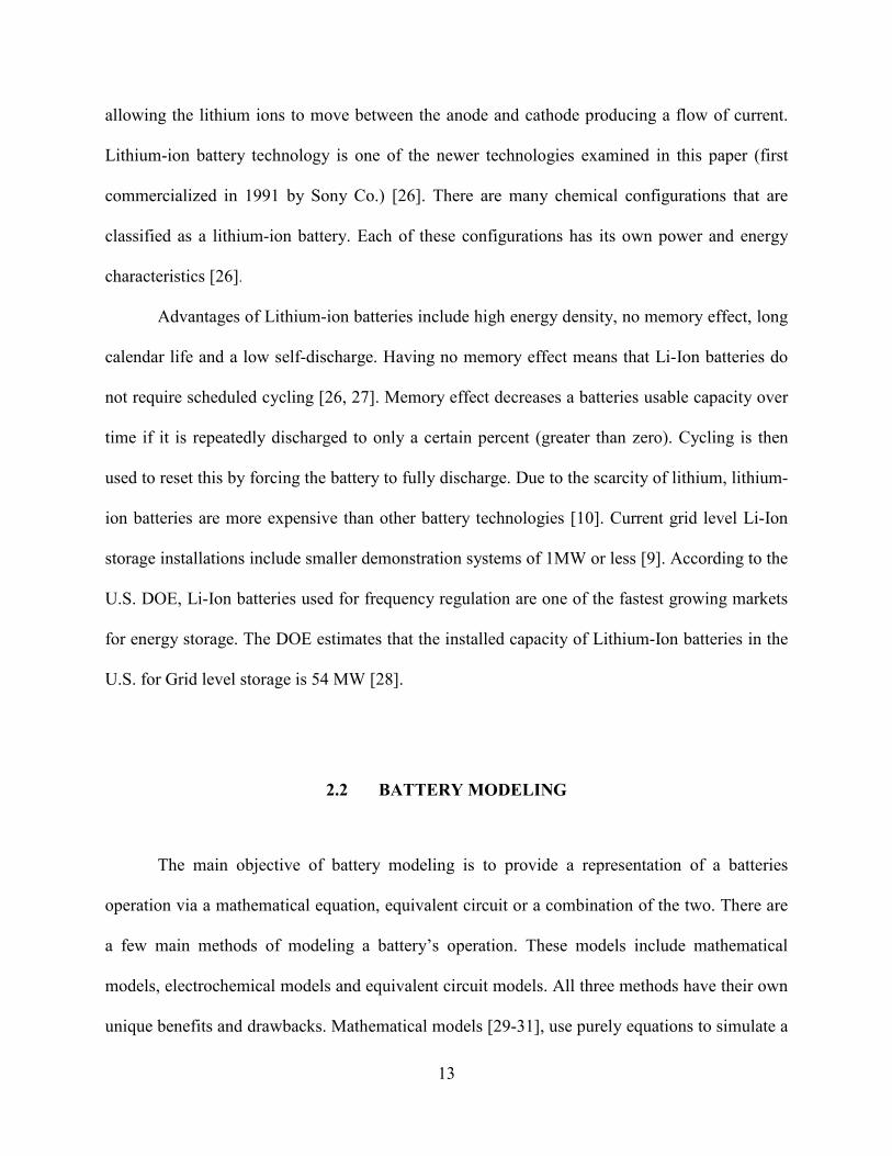
2.2 BATTERY MODELING
The main objective of battery modeling is to provide a representation of a batteries
operation via a mathematical equation, equivalent circuit or a combination of the two. There are
a few main methods of modeling a battery’s operation. These models include mathematical
models, electrochemical models and equivalent circuit models. All three methods have their own
unique benefits and drawbacks. Mathematical models [29-31], use purely equations to simulate a

14
battery’s operation; however, these models are not able to provide the necessary I-V information
for system level simulation [32]. A secondary draw back in mathematical models is that their
steady state error is on the order of 5%-20%, the highest of the three examined models [32].
Electrochemical models [33-35], take into account the kinetics and thermodynamics of the
battery’s electrochemical reaction. They are highly complex and require days of simulation to
obtain an accurate result; however, they provide the most accurate steady state simulation [32].
Equivalent circuit models [36-40], provide a compromise between mathematical and
electrochemical models in terms of accuracy, between 1%-5% [32]. Equivalent circuit models
are presented in a way that is easy for electrical engineers to work and integrate with circuit
simulation programs.
Electrochemical Models 2.2.1
Electrochemical battery models use the chemical, thermodynamic, and physical qualities
of the battery and yield the most accurate results, at a sacrifice to simulation time [33-35, 41].
The Peukert relationship displayed in (2.1) is used to determine the state of charge, SOC, of a
battery with constant discharge rate [42].
KTI in =* (2.1)
where: • I is the discharge current in Amps • n is a battery constant determined by the battery technology • K is a fixed constant
Using the Peukert relationship, the battery capacity in ampere-hour at a given discharge
rate Ii can be related to a known discharge rate In, as shown by (2.2).

15
1)/( −= ninni IICC (2.2)
where: • Ci is the battery capacity in Ampere-hours • Cn is a known battery capacity in Ampere-hours • In is a known discharge rate in Amps • Ii is a given discharge rate in Amps • n is a battery constant determined by the battery technology
For a constant discharge rate, the SOC as a function of the present discharge rate and
capacity can be calculated using (2.3).
tICCCSOC
iDi
iDi
=−= /1
(2.3)
where: • Ci is the battery capacity in Ampere-hours • CDi is the capacity in Ampere-hours at discharge rate Ii and time t • Ii is a given discharge rate in Amps • SOC is the battery’s current state of charge
For a non-constant discharge rate, which is the case with a real world battery energy
storage system implementation, the SOC equation will change so that the relation is evaluated in
small time intervals, as shown by (2.4). SOCK (2.5) is the net state of charge at k-th time interval.
1
3600
−
∆−=∆
n
n
i
n
iK I
ICtI
SOC (2.4)
KKK SOCSOCSOC ∆+= −1
(2.5)
where: • Ii is a given discharge rate in Amps • In is a known discharge rate in Amps • Cn is a known battery capacity in Ampere-hours • n is a battery constant determined by the battery technology • SOCK is the net state of charge at the k-th interval

16
Equivalent Circuit Models 2.2.2
Equivalent circuit battery models are typically used for power system simulations. Due to
being composed of common circuit components such as voltage sources, resistors and capacitors;
equivalent circuit battery models are easier for electrical engineers to work with. There are two
main types of equivalent circuit battery models, static and dynamic. Static battery models use
predetermined and constant battery characteristics throughout the entire simulation. In a dynamic
battery model, the battery voltage, current, charge, and temperature all vary as a function one
another which dynamically affects the output.
The most basic equivalent circuit model for batteries is the ideal circuit model shown in
Figure 2-4. This model is characterized by a voltage source only, and does not represent internal
battery characteristics [38].
EMF
+
Vo
-
Figure 2-4. Ideal battery equivalent circuit model
The linear model, Figure 2-5, expands upon the ideal circuit model by adding a resistor in
series with the voltage source. This resistor, Rint, represents the internal resistance of the battery.
The voltage source, EMF, is the no load voltage of the battery. This model can be improved by
making the values of Rint and EMF dependent upon the battery SOC instead of fixed values [38].

17
EMF
+
Vo
-
Rint
Figure 2-5. Linear battery equivalent circuit model
The Thevenin Model, Figure 2-6, includes the ideal no load voltage, EMF, the battery
internal resistance, R2, as well as the addition of capacitance, C1, and an overvoltage resistance,
R1. Like the linear model, the Thevenin model’s accuracy can be improved by making the
parameters which determine the internal resistance and electromotive force variable and
determined by the battery current SOC [39]
EMF
+
Vo
-
Rint
R1
C1
Figure 2-6. Thevenin battery equivalent circuit model

18
3.0 SYSTEM LAYOUT AND DESIGN
This section presents the design and simulation of a common DC bus electric vehicle charging
station (EVCS) which uses solar power in conjunction with a tie to the MVDC network to charge
the EVs. The operation of the EVCS is evaluated with and without connection to the MVDC grid
model, shown in Figure 3-1. The design of the MVDC grid as a whole is not the focus of this
thesis and thus, the control and sizing of components is not discussed in detail. Further
information on the design and control of the larger MVDC grid is available in [4, 43].
DC / ACThree LevelMultilevel Inverter(NPC)
+ -MVDC
5 MW SupplyAC / DC
Three LevelMultilevel Rectifier(NPC)
AC / DCThree LevelMultilevel Rectifier(NPC)
DC Cable
MPPT EnabledPMSG Based
PMSG Based
3.3 kV / 33 kV
DC Electric Vehicle Charging Station
Industrial Facility
Voltage Regulator
5 MW Supply
MPPT Enabled
DC Cable
AC / DCThree LevelMultilevel Rectifier(NPC)
DC Cable5 MW Supply
MPPT EnabledPMSG Based
Figure 3-1. PSCAD MVDC Interconnected Model

19
3.1 MVDC NETWORK
The MVDC network serves as the main source of generation in the interconnected model. The
MVDC grid model, Figure 3-1, consists of three 5-MW permanent machine synchronous
generators (PMSG) connected to the DC bus via three level neutral point clamped (NPC)
rectifiers and DC cable. The industrial facility is modeled as two 10 kW induction machines
operating at 60 Hz each of which are interfaced via a three level NPC inverter. The bus reactive
power and voltage is regulated via the utility tie three level NPC inverter. The utility is
represented as an infinite bus which absorbs the excess power generated by the wind turbines.
Wind Power Generation Model Development 3.1.1
The first step in modeling a wind turbine generator is quantifying the mechanical power supplied
by the wind. The mechanical power supplied by the wind for a given area swept by a turbine is
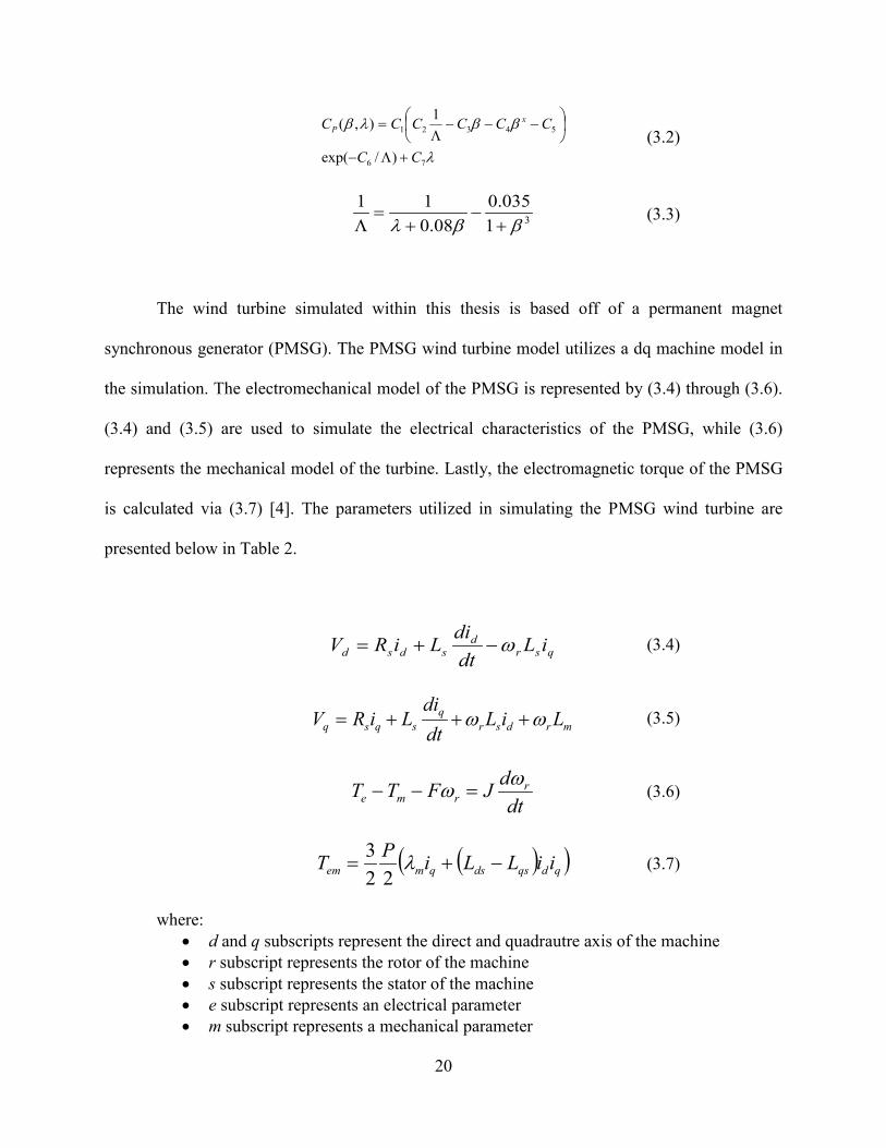
presented in (3.1). The power coefficient (CP), is presented in (3.2) and (3.3), the coefficients are
experimentally determined, C1 = 0.5176, C2 = 116, C3 = 0.4, C4 = 0, C5 = 5, C6 = 21, and C7 =
0.0068 [4].
3),(21
WVPACTP λβρ= (3.1)
where: • PT is the mechanical power supplied by the wind • ρ is the density of air • A is the area swept by the blades of the wind turbine • CP is an experimentally determined power coefficient • β is the pitch angle of the wind turbine blades • λ is the tip speed ratio of the wind turbine blades • VW is the wind velocity
20
λ
ββλβ
76
54321
)/exp(
1),(
CC
CCCCCC xP
+Λ−
−−−
Λ= (3.2)
31035.0
08.011
ββλ +−
+=
Λ (3.3)
The wind turbine simulated within this thesis is based off of a permanent magnet
synchronous generator (PMSG). The PMSG wind turbine model utilizes a dq machine model in
the simulation. The electromechanical model of the PMSG is represented by (3.4) through (3.6).
(3.4) and (3.5) are used to simulate the electrical characteristics of the PMSG, while (3.6)
represents the mechanical model of the turbine. Lastly, the electromagnetic torque of the PMSG
is calculated via (3.7) [4]. The parameters utilized in simulating the PMSG wind turbine are
presented below in Table 2.
qsrd
sdsd iLdtdiLiRV ω−+= (3.4)
mrdsrq
sqsq LiLdtdi
LiRV ωω +++=
(3.5)
dt
dJFTT rrme
ωω =−−
(3.6)
( )( )qdqsdsqmem iiLLiPT −+= λ22
3
(3.7)
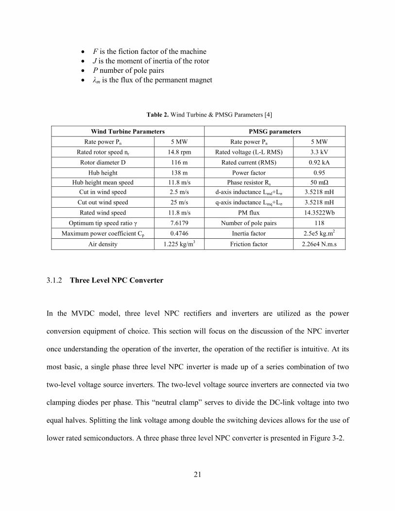
where: • d and q subscripts represent the direct and quadrautre axis of the machine • r subscript represents the rotor of the machine • s subscript represents the stator of the machine • e subscript represents an electrical parameter • m subscript represents a mechanical parameter
21
• F is the fiction factor of the machine • J is the moment of inertia of the rotor • P number of pole pairs • λm is the flux of the permanent magnet
Table 2. Wind Turbine & PMSG Parameters [4]
Wind Turbine Parameters PMSG parameters Rate power Pn 5 MW Rate power Pn 5 MW
Rated rotor speed nr 14.8 rpm Rated voltage (L-L RMS) 3.3 kV Rotor diameter D 116 m Rated current (RMS) 0.92 kA
Hub height 138 m Power factor 0.95 Hub height mean speed 11.8 m/s Phase resistor Rs 50 mΩ
Cut in wind speed 2.5 m/s d-axis inductance Lmd+Lσ 3.5218 mH Cut out wind speed 25 m/s q-axis inductance Lmq+Lσ 3.5218 mH Rated wind speed 11.8 m/s PM flux 14.3522Wb
Optimum tip speed ratio γ 7.6179 Number of pole pairs 118 Maximum power coefficient Cp 0.4746 Inertia factor 2.5e5 kg.m2
Air density 1.225 kg/m3 Friction factor 2.26e4 N.m.s
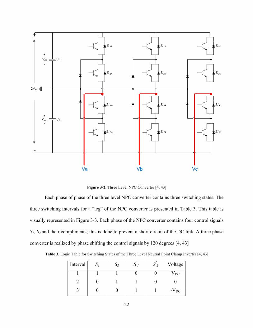
Three Level NPC Converter 3.1.2
In the MVDC model, three level NPC rectifiers and inverters are utilized as the power
conversion equipment of choice. This section will focus on the discussion of the NPC inverter
once understanding the operation of the inverter, the operation of the rectifier is intuitive. At its
most basic, a single phase three level NPC inverter is made up of a series combination of two
two-level voltage source inverters. The two-level voltage source inverters are connected via two
clamping diodes per phase. This “neutral clamp” serves to divide the DC-link voltage into two
equal halves. Splitting the link voltage among double the switching devices allows for the use of
lower rated semiconductors. A three phase three level NPC converter is presented in Figure 3-2.
22
Figure 3-2. Three Level NPC Converter [4, 43]
Each phase of phase of the three level NPC converter contains three switching states. The
three switching intervals for a “leg” of the NPC converter is presented in Table 3. This table is
visually represented in Figure 3-3. Each phase of the NPC converter contains four control signals
S1, S2 and their compliments; this is done to prevent a short circuit of the DC link. A three phase
converter is realized by phase shifting the control signals by 120 degrees [4, 43]
Table 3. Logic Table for Switching States of the Three Level Neutral Point Clamp Inverter [4, 43]
Interval S1 S2 S’1 S’
2 Voltage
1 1 1 0 0 VDC
2 0 1 1 0 0
3 0 0 1 1 -VDC

23
Figure 3-3. Three-Level Neutral Point Clamped Converter Single Phase Switching States [4, 43]
Industrial Facility 3.1.3
In the MVDC system model, the industrial facility represents the other load in the system. The
industrial facility is modeled using two 10-kW, 460 V (line-to-line rms), three phase, 4-pole
induction machines each powered via a three level NPC inverter. The inverter output is
3.3 kVL-L which is then stepped down via a transformer to the 460 VL-L power needed for the
machine. In this model the inverter is operating similarly to a drive. However, the inverter does
not possess the controls necessary to provide regulation and correction beyond steady state feed
forward control.
The induction machine parameters used in this simulation are presented in Table 4. These
parameters provide the per unit values for the per-phase induction machine equivalent circuit
presented in Figure 3-4. In this equivalent circuit, the components specified with a subscript one
represent stator components and components with a subscript two represent rotor components.
S1A
S2A
S’1A
S’2A
C1
C2
Vdc
+
+
-
-
+
-
2Vdc
Vdc
S1A
S2A
S’1A
S’2A
C1
C2
Vdc
+
+
-
-
+
-
2Vdc
Vdc
S1A
S2A
S’1A
S’2A
C1
C2
Vdc
+
+
-
-
+
-
2Vdc
Vdc

24
Utilizing the per-phase equivalent circuit shown above in Figure 3-4, the machines electrical
power (Pe), mechanical power (Pmech), and electromechanical torque (Te) can be calculated.
Table 4. Induction Machine Equivalent Circuit Parameters [43]
Stator Resistance (R1) 0.025
Referred Resistance (R2) 0.030
Stator Reactance (X1) 0.10
Referred Reactance (X2) 0.10
Magnetizing Resistance (RM) 20
Magnetizing Reactance (XM) 2.4
R1
+Vφ
jX1-
RM jXM
jX2
R2/s
Figure 3-4. Per-Phase Equivalent Circuit of an Induction Motor [44]
3.2 EV CHARGING STATION
Traditional level 2 DC quick charge electric vehicle charging stations (EVCS) utilize a common
AC bus architecture, which rectifies power for charging the electric vehicles [7]. An alternative
architecture rectifies the power at the input of the charging station and utilizes a common DC bus
throughout the EVCS [45, 46]. The system evaluated in this thesis, shown in Figure 3-5, utilizes
the common DC bus idea [45-47]. However, this simulation expands upon the idea through

25
connection of the system to a larger MVDC bus via a bidirectional DC-DC converter. A second
deviation is through use of detailed and accurate models of power converters as well as the use
of the PSCAD simulation environment, which allows simulation at a much smaller time step
(12μs was used in all experimentation) to more accurately capture the operation of the power
electronic conversion devices and allow for transient level evaluation.
Design Criteria for the EV Charging Station 3.2.1
The modeled system, Figure 3-5, consists of a 20 kW solar array, two level 2 DC fast chargers
and a tie to the MVDC network via a bidirectional DC-DC converter, which allows for the
EVCS to operate as a source of generation when no load is present. This study investigates the
power conversion infrastructure present within the EVCS as well as its interaction with the larger
MVDC network.
The use of a LVDC bus in the EVCS allows for greater system efficiency by removing
the inversion step which would otherwise be necessary at the output of the solar panels. The DC
EVCS also reduces footprint by replacing the large 60Hz input transformer with a smaller high
frequency transformer present within the bidirectional DC-DC converter while still providing
galvanic isolation. Figure 3-6 presents a typical EVCS with roof mounted solar panels. A bus
voltage of 800 VDC was chosen for the LVDC bus. A standard LVDC bus voltage has not been
determined and many voltage levels exist in literature [48-50]. The DC bus was grounded via
capacitive coupling at the sources and loads as described in [51].

26
+ -
LVDC800 VDC
Voltage Regulator
Bi-DirectionalDC / DC
Converter
MVDCNetwork
20 kW PV
Boost Converter
SynchronousBuck
SynchronousBuck
Constant Current Control
MPPT Enabled
Linear Battery
Linear Battery
Constant Current Control
Figure 3-5. Electric Vehicle Charging Station One Line Diagram
Figure 3-6. Electric Vehicle Charging Station with Solar Generation [52]

27
The designed system utilizes level 2 DC vehicle charging. Level 2 DC charging utilizes
50-70 kW of charging power and is capable of fully charging an electric vehicle in 15-50
minutes. Current charging systems are classified as level 1 and level 2 AC. Level 1 AC charges
at 1.4 kW and takes 18 hours to charge. Level 2 AC chargers provide 3.3 or 6.6 kW of power and
takes 8 or 4 hours to charge respectively [7, 53, 54]. At 50 kW of charging power, a level 2 DC
fast charger will almost exclusively be installed at commercial / industrial locations, such as the
system presented in this study.
Bidirectional DC-DC Converter 3.2.2
The bidirectional DC-DC converter allows for a bidirectional flow of power to utilize grid power
when necessary and to supply power to the grid when excess power is generated, shown in
Figure 3-7. Applications of bidirectional DC-DC converters include battery energy storage
systems, next generation motor drives, interconnecting load centers that possess on site
generation [48, 55-57]. The bidirectional DC-DC converter used in this section is based off of
the one designed in [48, 57].
In this chapter the bidirectional DC-DC converters operation within the context of the
EVCS, Figure 3-5, will be considered. In buck mode, the bidirectional DC-DC converter, Figure
3-7, utilizes constant voltage control to operate as a voltage regulator for the LVDC bus.

28
C1
1 : nLLK
L
VLV
+
-
S1
S2
S3
S4
S5
S6
S7
S8
C2VHV
+
-
Boost Mode Buck Mode
Bidirectional Power Flow IHVILV
EP ES+
-
+
-
Figure 3-7. Bidirectional DC-DC Converter
The gating signals and key operating waveforms as well as the converter current paths for
the boost and buck modes of operation for the bidirectional DC-DC converter are presented in
Figure 3-8, Figure 3-9, Figure 3-10, and Figure 3-11 respectively. The currents IHV and ILV are
measured using the reference of ‘going into the converter’ as the positive direction, which is why
IL is negative in buck mode and positive in boost mode. In boost mode only one current wave
form is displayed, Figure 3-8, because the ideal input current is also the inductor current. IHV
represents the current entering/leaving the high voltage side of the converter, ILV is the current
entering/leaving the low voltage side of the converter and IL is the current through the choke
inductor, L. The gating signals shown in Figure 3-8 and Figure 3-10 are based off of those
presented in [57].

29
DTS (1-D)TS
S1 & S2
S3 & S4
Boost Mode
ES/n=EP
I LV =I L
TS 3TS2TS0
Figure 3-8. Bidirectional DC-DC Converter Boost Mode Operating Waveforms
In boost mode the bidirectional DC-DC converter increases the input voltage from the
LVDC bus voltage of 800V to the MVDC bus voltage of 4.25 kV. As shown in Figure 3-9
switches 1, 2, 3, and 4 are used to generate a sinusoidal waveform which is then rectified via
blocks 5, 6, 7, and 8. In interval 1 the flow of current is shown in Figure 3-9A. During intervals 1
and 3, switches 1, 2, 3, and 4 are all on and power is stored in the choke inductor (L). In interval
2, Figure 3-9B, switches 1 and 2 turn off and power is transferred from the low voltage side
through the transformer, rectified via blocks 7 and 8 and transferred into the load. Interval 4,
Figure 3-9C, once again transfers power stored in the choke inductor to the load.

30
(A) Interval 1: 0 < t < DTS / Interval 3: TS < t < (TS + DTS)
(B) Interval 2: DTS < t < TS
(C) Interval 4: (TS + DTS) < t < 2TS
Figure 3-9. Boost Mode Converter Current Paths for Operating States

31
(1-D)TSDTS
S5 & S6
Buck Mode
S7 & S8
ES/n=EP
I HV
I L
TS 3TS2TS0
Figure 3-10. Bidirectional DC-DC Converter Buck Mode Operating Waveforms
In buck mode the bidirectional DC-DC converter reduces the input voltage from the
MVDC bus voltage of 4.25 kV to the LVDC bus voltage of 800 V. As shown in Figure 3-10,
switches 5, 6, 7, and 8 are used to generate a sinusoidal waveform which is then rectified via
blocks 1, 2, 3, and 4. In interval 1 the flow of current is shown in Figure 3-11A. During interval
1, power is transferred from the high voltage side through the transformer and stored in the
choke inductor (L). In Interval 2 and 4, Figure 3-11B, all switches are off and power is cycled
through the primary side of the circuit and onto the LV bus. Interval 3, Figure 3-11C, once again
transfers power from the high voltage side of the circuit and stores it in the choke inductor.

32
(A) Interval 1: 0 < t < DTS
(B) Interval 2: DTS < t < TS / Interval 4: (TS + DTS) < t < 2TS
(C) Interval 3: TS < t < (TS + DTS)
Figure 3-11. Buck Mode Converter Current Paths for Operating States

33
In order to predict the steady state output of the converter, inductor volt-seconds balance,
capacitor charge balance, and the small-ripple approximation are utilized in determining the
average output voltage and current [58]. Analysis is performed using the buck mode operating
states presented in Figure 3-11. During interval 1, Figure 3-11A, KVL was performed to
calculate the voltage across the choke inductor (vL), (3.8). KCL was performed at the node above
C1 to calculate the current through the capacitor (iC), (3.9)
LVHV
L Vn
Vv −= (3.8)
RVIiC −= (3.9)
During interval 2, Figure 3-11B, KVL and KCL were again performed at the same points
yielding the voltage across the choke inductor, (3.10), and the current through the capacitor,
(3.11).
LVL Vv −= (3.10)
RVIiC −= (3.11)
Performing, KVL and KCL during interval 3 Figure 3-11C, and interval 4, Figure 3-11B,
yields the same results as in (3.8) / (3.9) and (3.10) / (3.11) respectively. Utilizing the properties
of volt-seconds balance and capacitor charge balance the average inductor voltage, <vL> and
average capacitor current, <iC>, are calculated. Equation (3.12) shows the calculation of average
inductor current over one switching period, which is then employed to calculate the output
voltage VLV, (3.13), given the input voltage (VHV), the duty cycle (D), and the transformer turns
ratio (n).

34
∫=⟩⟨ST
LS
L dttvT
v0
)(1
( )
S
SLVSLVHV
L T
TDVDTVn
V
v'−+
−
=⟩⟨
(3.12)
n
DVV HVLV = (3.13)
The calculation of average capacitor current over a switching period is shown in equation
(3.14). (3.15) is simplified to calculate the DC value of the inductor current (I), given the output
voltage (VLV) and the load resistance (R).
∫=⟩⟨ST
CS
C dttiT
i0
)(1
S
SS
C T
TDRVIDT
RVI
i'
−+
−
=⟩⟨
(3.14)
R
VI LV= (3.15)
In buck mode, the bidirectional DC-DC converter provides voltage regulation for the
LVDC bus. The regulation is accomplished utilizing voltage feedback control, Figure 3-12. The
controller measures the LVDC bus voltage and compares it to a reference value. A PI block is
used to adjust the converters steady-state error and response time. A reference carrier operating
at (TS/2) compared with the PI blocks output is used to generate the systems gating signals

35
+-
Vref = 800 V
P
I Comparator
Carrier
Gate Drive
LVDC Bus Measurement
+
Figure 3-12. Controller for Bidirectional DC-DC Converter Buck Mode Voltage Regulation
In the interconnected model, due to limited power within the system, the need for a pre-
charge circuit was emphasized. The pre-charge circuit limits the input capacitor’s (C2) inrush
current, which is needed due to the fact that an uncharged capacitor behaves as a short circuit,
which in turn leads to a collapse of the MVDC bus. In this simulation the simplest form of pre-
charge circuit is utilized. Two resistors are added in series with the capacitor, Figure 3-13, to
limit the inrush current and are removed via a switch once the DC link capacitor reaches the
appropriate level of charge. Also, notice the addition of the damping circuit to the bidirectional
dc-dc converter shown in Figure 3-13, the damping circuit consisting of a damping resistor
(RDamp) and a controlled switch (SD), which is used to actively limit the bus voltage during
transient loss of load and steady state no load conditions, minimizing overshoot and steady state
error. Table 5 contains the operating parameters of all components in the bidirectional DC-DC
converter, these components are based off of the values presented in [48].

36
C1
1 : nLLK
L
VLV
+
-
S1
S2
S3
S4
S5
S6
S7
S8
C2 VHV
+
-
RLim
RPreRDamp
SD
Figure 3-13. Bidirectional DC-DC Converter with Pre-charge Circuit and Damping Circuit
Table 5. Operating Parameters Bidirectional DC-DC Converter
Choke Inductance (L) 1 mH
Leakage Inductance (LLK) 27 μH
Low Voltage Filter Capacitor (C1) 2 mF
High Voltage Filter Capacitor (C2) 2.7 mF
Pre-charge Resistor (RPre) 47 Ω
Inrush Limit Resistor (RLim) 25 Ω
Damping Resistor (RDamp) 11 Ω
Transformer Turns Ratio (n) 3
Synchronous Buck Converter 3.2.3
The synchronous buck converter is used to simulate the battery charger in the electric vehicle
charging station model. The synchronous buck converter, Figure 3-14, is used to regulate the
charging power at the desired level (in the case of level 2 DC fast charging, 50 kW). The
synchronous buck converter operates similarly to a traditional buck converter. The main
difference being that, rather than using a diode to naturally commutate during the D’ section of
the switching period, a second switch (S2) is used, graphically portrayed in Figure 3-16. To

37
regulate charging power at 50 kW the synchronous buck converter utilizes constant current
feedback control, shown in Figure 3-15.
C
LVHV
+
-
S1
S2 VLV
+
-
Figure 3-14. Synchronous Buck Converter
+-
Iref = 125 A
N/DP
I Comparator
Carrier
Gate Drive
Synch Buck Output Current Measurement
+
Figure 3-15. Constant Power Feedback Controller
DTS (1-D)TS
S1
S2
VLV
I LV =I L
TS 2TS0
Figure 3-16. Key Operating Waveforms of Synchronous Buck Converter

38
The main benefit of using a synchronous buck converter over a regular buck converter is
the reduced conduction losses due to the use of IGBTs during both portions of the switching
period [59]. An example of a synchronous buck converter being used for EV battery charging is
implemented in hardware and presented in [60]. The values of L (25.3303 mH) and C (1 μF)
were chosen such that they would filter out harmonic content above 1 kHz, according to (3.16),
(3.17), and (3.18).
22
2
)( o
o
in
O
jVV
ωωω+
= (3.16)
LCo12 =ω (3.17)
=LPfLCπ2
1 (3.18)
where: • ωo is the cutoff frequency of the filter in rad/s • fLP is the cutoff frequency of the filter in Hz
Electric Vehicle Linear Battery Model 3.2.4
The level 2 DC fast charging is anticipated to be a game changer in the EV industry [53].
Traditional EV charging methods such as level 1 and 2 chargers take between four and sixteen
hours to fully charge a depleted battery, which is only feasible for overnight or at work charging.
Level 2 DC fast chargers allow for charging of a EVs battery in as little as fifteen minutes [53].
A 50 kW level 2 fast charger operating at 400 VDC will have a charging current of 125 ADC.
An example charging profile of a lithium-ion phosphate (LFP) battery which are widely
used in automotive applications is presented in Figure 3-17 [54]. A typical battery charge cycle

39
consists of two modes constant current (CC) charging and constant voltage (CV) charging. For a
LFP battery used in automotive applications the CC charging time takes 75% of the total
charging time and reaches a SOC of approximately 95%. The remaining 25% of the charge time
the battery is charged utilizing CV charging. From inspection of the charging profile presented in
Figure 3-17, that maximum charging power occurs at the end of CC charging, for this reason the
battery charging simulation assumes 90% SOC.
Figure 3-17. Charging Profile for a Lithium-Ion Phosphate Battery [54]
The electric vehicle battery is represented using a linear battery model. The simulation
assumes that all vehicles have the same size battery (22.1 Ah). As explained earlier to maximize
system load the simulation assumes that the EV batteries are at the end of the CC charging cycle
at 95% state of charge. Due to the size and complexity of the entire EVCS and MVDC model,
the simulation is only run for a few seconds (2.1 seconds), and during those few seconds the

40
battery is charged for approximately 1.0 second. As shown in Figure 3-17, over any one second
interval, the charging of a lithium-ion phosphate battery can be approximated as being linear.
The linear battery model used in this simulation, Figure 3-18, consists of a dependent voltage
source (EMF) in series with a variable resistance (Rint).
+-
RINT
EMF VBAT
+
-
IBAT
Figure 3-18. Electric Vehicle Linear Battery Model
The linear battery model is designed to have a fully charged terminal voltage of 600 VDC
and charge at around 88.3 ADC. Due to constant power charging, the battery will have a higher
current at the beginning of charge due to a lower terminal voltage. The electromotive force
(EMF) and internal resistance (Rint) both adjust linearly as a function of the battery’s state of
charge as shown in (3.19), (3.20), (3.21), and (3.22). State of charge refers to the percentage full
the battery is, a SOC of 0.5 represents a battery that is 50% full. The values for Vmin (battery
voltage at 0% SOC), Rint (battery internal and terminal resistance), KV, and KR (constants
determined by battery type) were approximated to yield the desired operation.

41
)(EMF Vmin SOCKV += (3.19)
)( Rminint SOCKRR += (3.20)
∫−=t
bate dIQ0
)( ττ (3.21)
max
SOCCQe= (3.22)
The values of EMF and Rint are both functions of the battery’s state of charge (SOC). The
battery’s extracted charge, Qe, and SOC are calculated via (3.21) and (3.22). Cmax is the battery’s
maximum capacity in Amp-seconds. The linear battery model parameters are presented in Table
6.
Table 6. Operating Parameters Linear Battery Model
Capacity 22 Ah
Vmin 366 V
Rmin 1 mΩ
Kv 0.34
Kc 90*10-6
Photovoltaic Array and Boost Converter 3.2.5
In the electric vehicle charging station model a roof mounted photovoltaic array is modeled and
simulated. The PV array serves as a source of on-site generation for the EVCS. The PV array is
simulated at the module level, via representation as a current source in antiparallel with a diode
and a resistance followed by a resistor in series, Figure 3-19. The equivalent circuit
representation of the PV module allows for a piece-wise linear approximation of the PV
module’s V-I curve. The piece-wise linear approximation allows for accurate simulation at key

42
operating points along the V-I curve. The comparison of the theoretical V-I curve and the one
approximated using the equivalent circuit, shown in Figure 3-19, is shown below in Figure 3-20
[4].
Figure 3-19. PV Array equivalent circuit model [4]
0 5 10 15 20 250
1
2
3
4
5
6
7
8
Voltage (V)
Cur
rent
(A)
TheoreticalSandia Model Using Key PointsPSCAD Implementation
Figure 3-20. Comparison of theoretical and simulated V-I curves for a single PV module [4]
The PV array in the EVCS was designed to output 20 kW. The design specification of the
solar modules were taken from production solar panels [61]. The relevant information from the
datasheet is presented below in Table 7.

43
Table 7. Kyocera Solar KC125G Module [61]
Parameter Descriptor Parameter Value
Short-Circuit Current Isc = 8.0 A
Current at 0.5Voc Ix = 7.86 A
Current for maximum power point Imp = 7.2 A
Current at 0.5(Voc + Vmp) Ixx = 5.1 A
Open-circuit Voltage Voc = 21.7 V
Voltage for maximum power point Vmp = 17.4 V
Number of modules in series to get Voc Nsbase = 36
Series resistance of the Sandia model Rs = 0.4216 Ω
Shunt resistance of the Sandia model Rsh = 77.5 Ω
The output of the PV array is scaled utilizing scaling factors ns and np which represent the
number of modules connected in series and parallel respectively. The PV array was designed to
have a 600 VDC output voltage, and output 20 kW. The output current of the PV array was
calculated at 33.3 ADC utilizing P=VI. Each series string of modules produces 17.4•nS VDC and
each string of modules configured in parallel produces 7.2•nP ADC [4].The calculation of ns and
np is shown in equations (3.23) and (3.24).
3548.34V4.17V600 n
DC
DCS ≈== (3.23)
562.4A2.7A33.3 n
DC
DCP ≈== (3.24)

44
The output of the PV array is conditioned to the proper voltage level for interconnection
into the LVDC bus (800 VDC) via a boost converter. The boost converter utilizes a maximum
power point tracking (MPPT) algorithm to maintain maximum power output of the PV array at a
constant 20 kW. The incremental conductance MPPT algorithm was chosen as the method of
MPPT to be utilized in the PV array. According to literature the incremental conductance MPPT
is an adequate and superior method of MPTT [62, 63]. Figure 3-21, presents a flow chart of the
incremental conductance MPPT algorithm utilized [63]. The incremental conductance algorithm
operates by determining the point where the derivative of the power curve for the PV array is
zero, which indicates the point of maximum power. The value of L and C were set to 10 mH and
1 mF respectively, these values were chosen to minimize output ripple.
Figure 3-21. Incremental Conductance Maximum Power Point Tracking Algorithm [63]d
45
4.0 PSCAD COMPONENT VALIDATION
In this chapter individual components within the MVDC, Figure 3-1, and EVCS, Figure 3-5,
system models are built within the PSCAD/EMTDC simulation environment and their operation
is validated in accordance with the predicted results presented in chapter 3.
4.1 MVDC SYSTEM COMPONENT VALIDATION
Within the MVDC system, the operation of three major components is discussed in chapter 3,
and are thus explored and validated in this section, the 5 MW permanent machine synchronous
generator (PMSG) wind turbine, the three level neutral point clamped (NPC) converter, and the
10 kW induction machine utilized in the industrial facility model. The design and operation of
the MVDC grid is not the primary focus of this thesis and as such will not be discussed in the
level of depth and detail that the electric vehicle charging station and related models will. More
information on the modeling of the MVDC system components can be found in [4].
5 MW PMSG Wind Turbine 4.1.1
Figure 4-1, shows the mechanical and electrical output power of one wind turbine verifying the 5
MW output power in the interconnected model. In the simulation the 5 MW PMSG wind

46
turbines are all designed to operate at their maximum output power and do not vary during
simulation. As such, all three wind turbines have the same output as the one presented in Figure
4-1.
0 0.2 0.4 0.6 0.8 1 1.2 1.4 1.6 1.8 2-2
-1
0
1
2
3
4
5
6
7
Pow
er (M
W)
Time (Seconds)
Mechanical PowerElectrical Power
Figure 4-1. Mechanical and Electrical Output Power of Permanent Machine Synchronous Generator
Three Level NPC Converter 4.1.2
Figure 4-2, displays the line-to-line input voltage of the three level NPC rectifiers. The number
of steps in the line-to-line voltage for an n level NPC converter, can be determined as 2n-1. Since
the converter utilizes a three topology, the expected number of steps is 5 [4].

47
0.62 0.64 0.66 0.68 0.7 0.72-6
-4
-2
0
2
4
6
Time (s)
Vol
tage
LL (k
V)
Figure 4-2. Line-to-Line Input Voltage of Three Level NPC Rectifier
10 kW Induction Machine 4.1.3
Figure 4-3, provides a graph showing the instantaneous power into the induction machine during
simulation. The breakers to the industrial facility close at 0.5 seconds connecting the industrial
facility to the MVDC grid, which is why the power is zero before 0.5 seconds. Notice that the
machine quickly regulates to a steady state value of 10 kW as desired. The industrial facility
contains two 10 kW induction machines and each operates in the same manner.

48
0 0.2 0.4 0.6 0.8 1 1.2 1.4 1.6 1.8 2-15
-10
-5
0
5
10
Pow
er (k
W)
Time (s)
Figure 4-3. Instantaneous Power Absorbed by Each Induction Machine
4.2 EVCS SYSTEM COMPONENT VALIDATION
Within this section, the operation of the PSCAD based models of the individual components
within the electric vehicle charging station (EVCS) is validated. The modeling and operation of
five main components is discussed and validated in accordance with the operation described in
chapter 3. These five main components include the bidirectional DC-DC converter, the
synchronous buck converter, the linear battery model, the boost converter, and the photovoltaic
array. Figure 4-4, shows the PSCAD model of the EVCS. Each of the individual components is
represented as a page module. The model shown in Figure 4-4 is specifically for the non-
interconnected case; however, in the interconnected model the ideal voltage sources at high side

49
of the bidirectional DC-DC converter are replaced with connections to the MVDC bus. The 1 nΩ
resistors throughout the model are added so that certain nodes are not shorted. The DC system is
grounded via capacitive coupling on both the positive and negative rails at all sources and loads.
Figure 4-4. EVCS PSCAD Implementation
Bidirectional DC-DC Converter 4.2.1
The bidirectional DC-DC converter is analyzed analytically in section 3.2.2, this section serves
to validate the operation of the bidirectional DC-DC converters buck mode of operation in
PSCAD utilizing the theoretical analysis performed in section 3.2.2. The waveforms presented in
this section are compared against the ones theoretically predicted in Figure 3-10. Figure 4-5,

50
shows the bidirectional DC-DC converter as it was represented in PSCAD as well as where
measurements were performed. Notice that the inrush and pre-charge resistors were represented
as variable resistances. After the DC link capacitor C2 reaches a desired level of charge they are
changed to 1 nΩ, essentially a short circuit.
Figure 4-5. Bidirectional DC-DC Converter PSCAD Implementation
The contestant voltage feedback controller is implemented in PSCAD as shown in Figure
4-6. In buck mode, the LV side of the converter is used as a passive rectifier and the IGBTs are
set to off the entire time. The HV side utilizes PWM to generate the desired AC wave. The time
delay block is utilized so that S7 and S8 actuate exactly one switching period after S5 and S6.
Figure 4-6. Bidirectional DC-DC Converter Buck Mode Constant Voltage Controller
As derived in section 3.2.2, the equation determining the average output voltage (VLV)
given a set input voltage (VHV), duty cycle (D) and turns ratio (n) is (4.1). (4.1) can be rewritten
as (4.2) to allow for the calculation of the duty cycle. Using VLV = 800 V, VHV = 4.25 kV, and n =
3, D is calculated using (4.2) to be 0.565.

51
n
DVV HVLV = (4.1)
HV
LV
VnVD = (4.2)
Figure 4-7, shows the gating signals for the buck mode operation of the converter during
steady state operation. Using the gating signals from the steady state operation of the PSCAD
model of the converter, the duty cycle is measured to be 0.552. This is close to the theoretically
calculated value of 0.565. The difference is caused by the fact that at steady state the converter
has a low frequency ripple, caused by various interacting controllers and system dynamics, super
imposed over the high frequency (2 kHz) switching ripple.
Figure 4-7. Buck Mode Gating Signals
The primary (EP) and secondary (ES) winding voltages across the high frequency
transformer are presented in Figure 4-8. During the “ON” period of the high voltage side
switches, a +/- VHV is applied across the primary winding of the transformer. When S5 & S6 are
DTS

52
“ON” a + VHV is applied across EP and during the next switching period when S7 & S8 are
“ON” a - VHV is applied across EP. In the simulated cases VHV is 4.25 kV. The voltage across
the secondary winding should be EP/n, in the case of the simulated converter, n is equal to 3,
meaning that ES should approximately be equal to 1.4 kV.
1.9938 1.994 1.9942 1.9944 1.9946 1.9948 1.995 1.9952 1.9954 1.9956-5
-4
-3
-2
-1
0
1
2
3
4
5
X: 1.994Y: 1.4
Vol
tage
(kV
)
Time (Seconds)
X: 1.994Y: 4.249
EpEs
Figure 4-8. Primary Side Voltage (EP) and Secondary Side Voltage (ES)
Figure 4-9, presents the choke inductor current ripple over four periods of operation.
When the “ON” interval of the switching period, either S5 & S6 are “ON” or S7 & S8 are “ON”, the
inductor current decreases about 180 A from a peak of approximately 190 A to a minimum of
approximately 13 A. Then during the “OFF” interval the current increases by approximately the
same amount so that the average current over any one period is zero maintaining the inductor
volt-seconds balance theory. Even though the system is operating at steady state in Figure 4-9,d
there is a low frequency ripple superimposed over the high frequency (2 kHz) switching ripple

53
which makes it so that between switching periods the converter does not reach the same peak
currents.
1.9938 1.994 1.9942 1.9944 1.9946 1.9948 1.995 1.9952 1.9954 1.9956-0.25
-0.2
-0.15
-0.1
-0.05
0 X: 1.994Y: -0.01389
Cur
rent
(kA
)
Time (Seconds)
X: 1.994Y: -0.1947
X: 1.995Y: -0.1956
Figure 4-9. Choke Inductor Current (iL)

54
The transformer leakage inductance current (iLK) is shown in Figure 4-10. The leakage
inductance current is non-zero only during the “ON” interval of the switching period and is
during that time the current that is flowing through the choke inductor. During the S5 & S6
“ON” intervals, the leakage inductor current is exactly equal to the choke inductor current.
Conversely, during S7 & S8 “ON” interval, the leakage inductor current is the negative of the
choke inductor current. This is caused by the polarity difference across the transformer which is
graphically represented via the operating paths shown in Figure 3-11.
1.9938 1.994 1.9942 1.9944 1.9946 1.9948 1.995 1.9952 1.9954 1.9956-0.25
-0.2
-0.15
-0.1
-0.05
0
0.05
0.1
0.15
0.2
0.25
X: 1.995Y: 0.1956
Cur
rent
(kA
)
Time (Seconds)
X: 1.994Y: -0.1947
Figure 4-10. Leakage Inductance Current (iLK)

55
The bidirectional DC-DC converters buck mode input current (iHV) over four switching periods is
presented in, Figure 4-11. The input current exists during the “ON” interval of the switching
period only, as illustrated in Figure 3-11. The current in the low voltage side of the circuit is
approximately equal to niHV.
1.9938 1.994 1.9942 1.9944 1.9946 1.9948 1.995 1.9952 1.9954 1.99560
0.01
0.02
0.03
0.04
0.05
0.06
0.07
0.08
0.09
0.1
X: 1.994Y: 0.06603
Cur
rent
(kA
)
Time (Seconds)
X: 1.995Y: 0.06687
Figure 4-11. High Voltage Side Input Current (iHV)
Synchronous Buck Converter 4.2.2
The theoretical operation of the synchronous buck converter is presented in section 3.2.3. This
section will show that the PSCAD implementation of the synchronous buck converter is in
agreement with the predicted theoretical operation. The PSCAD model for the synchronous buck
converter is presented in Figure 4-12. The one nΩ resistor is necessary so that the two electrical

56
connections HV_N and LV_N are not connected to the same node. When two electrical
connections are connected to the same node an error is created in PSCAD.
HV_P
HV_N
LV_P
LV_N
I
S1
S1a
I
S2
S2a
25.3303[mH]
1 [uF]
il
Vlv
Vhv
Io
D
D
1.0 [nohm]
Figure 4-12. Synchronous Buck Converter PSCAD Implementation
The synchronous Buck Converter utilizes constant current control to output the desired
charging current for the electric vehicle batteries. The feedback controller is also utilized to
generate the gating signals for the converter.
Figure 4-13. Synchronous Buck Converter Controller and Gating Signal Driver
The synchronous buck converter output voltage and current have a triangular ripple
which are both in phase and have a positive slope when S1 is “ON” and a negative slope when S2
is “ON”. This is illustrated in Figure 3-16. The synchronous converters output voltage is
presented in Figure 4-14, and the output current is presented in Figure 4-15. These operate as
expected and provide an average output power of approximately 50 kW.

57
Figure 4-14. Synchronous Buck Converter Output Voltage (VLV)
1.24 1.2402 1.2404 1.2406 1.2408 1.241 1.2412 1.2414 1.2416 1.2418 1.242122.5
123
123.5
124
124.5
125
125.5
126
126.5
127
127.5
X: 1.24Y: 127.1
Time (s)
Cur
rent
(A)
X: 1.24Y: 122.9
Figure 4-15. Synchronous Buck Converter Output Current (ILV)

58
Linear Battery Model 4.2.3
The linear battery model is used to simulate the battery of the electric vehicle. It is represented as
a variable voltage source in series with a variable resistance, both of which vary linearly with the
batteries present state of charge. The linear battery model is represented in PSCAD as shown in
Figure 4-16.
Rint1
+ Iout1
R=0V
EMF1N
D
N/D
1000.0
positive1
negative1
Vbat1
Figure 4-16. PSCAD Implementation of Linear Battery Model
The battery’s state of charge (SOC) is calculated in accordance with the equations
presented in section 3.2.4. Figure 4-17, is the PSCAD implementation of the equations presented
in section 3.2.4.
22.0Ah
*
3600.0s
A
B Compar-ator
1.0
BatF
ull1
Capacity1
Iout1*
-1.0 Qe1
N(s)D(s)
Order = 1Ima1
1000.0
* N
D
N/D SOC1
Figure 4-17. PSCAD Calculation of SOC
Figure 4-18 displays the voltage and current for a pulse charge on EV battery 2. The
pulse charge lasts for 0.55 seconds. During that time the battery charges at a constant current of
125 ADC and a voltage of about 394.25 VDC (49.3 kW) which is increasing linearly according to
the equations presented in section 3.2.4. This pulse charge is captured towards the end of

59
constant current charging at 95% SOC. A reference pulse charge is presented in Figure 4-19,
notice how the simulated pulse charge shown in Figure 4-18 matches the general shape of the
reference pulse charge. They two pulse charges are not meant to be representative of the same
battery the reference pulse charge (Figure 4-19) is charging at a different current, state of charge
and voltage than the simulation and will not match perfectly. Only the non-interconnected model
battery charging voltage and current is presented.
Figure 4-18. EV Battery 2 Pulse Charge Voltage and Current

60
Figure 4-19. Example Li-Ion Battery Pulse Charge [64]
Photovoltaic Array 4.2.4
The PV array and boost converter are modeled in PSCAD as shown below in Figure 4-20. The
PV array component is a modified version of the generic model shown in Figure 3-19. The three
anti-parallel diodes in combination with their parallel resistors are tuned to provide accurate
operation and key operating points along the PV’s output curve, Figure 3-20. The operation of
the PV array is validated in more detail in [4].
D
D
D
Rs
+
Rsh +
Rtop +
Rm
id +
Isc
D
0.01 [H]
D
D1
Ipv
Vpv
1000.0 [uF]
Figure 4-20. PV Array and Boost Converter PSCAD Implementation

61
The incremental conductance MPPT algorithm was implemented in PSCAD utilizing
logic gates as shown in Figure 4-21. The MPPT algorithm is used to calculate the reference
voltage which is utilized in determining the duty cycle of the boost converter tied to output of the
PV array.
Vpv
Ipv
Vref
D +
F
-
D +
F
-
B+
D +
F
+
YES
NOYES
NO
delta_V = 0, delta_I != 0
delta_I > 0
delta_I < 0
B+
F
+
*
*
Vref_inc
Vref_inc
*-1.0
delta_V != 0
N
D
N/D
Vpv
IpvN
D
N/D
*-1.0
Vref_inc
*
*
E
+
F
+ d_I/d_V = -I/V
A
B Compar-ator
Vref_inc
*-1.0
del_V
del_I
del_V
del_I
D +
F
+
Vref_fdbk
d_I/d_V > -I/Vd_I/d_V < -I/V
delta_V = 0
delta_I > 0
delta_I = 0
Figure 4-21. PSCAD Implementation of Incremental Conductance Algorithm

62
Figure 4-22, below shows the output power of the PV array and boost converter in a test
system across a 100 Ω load resistor. The PV array output power is slightly higher than the
designed 20 kW more around 21 kW. This is due to rounding up of the number of series
connected panels. In accordance with the equations in section 3.2.5, the theoretical output power
of the PV array is 17.4•nS•7.2•np=21.9 kW (np=5 and ns=35).
0 0.1 0.2 0.3 0.4 0.5 0.6 0.7 0.8 0.9 10
2
4
6
8
10
12
14
16
18
20
22
Time (s)
Pow
er (k
W)
Figure 4-22. PV Array Output Power Test System

63
5.0 SYSTEM ANALYSIS, OPERATION, AND RESULTS
In Chapter 5, the system level interaction and operation of the electric vehicle charging station
with and without interconnection to the full MVDC network will be evaluated during the EVCSs
various modes of operation. The electric vehicle charging station has two primary modes of
operation, when serving purely as a load (charging of electric vehicles and PV array ON or OFF)
and when acting as a source of generation (no EVs present and PV array ON). In this chapter,
two models will be referenced, the interconnected model, in which the EVCS is connected to the
MVDC grid model, and the non-interconnected model, in which the MVDC grid is represented
by an ideal voltage source. The two different models are utilized to validate the use of an ideal
voltage source as an appropriate representation of the MVDC grid to allow for quicker and more
intricate simulations, as well as determine what problems are unique to the MVDC grid model
containing realistic generation sources. In, section 5.2 effect of the battery chargers (synchronous
buck converter) operation during a battery pole to pole (short circuit) fault is explored. In
particular the ability of the converter to block or propagate the transmission of faults based off of
the power electronic switching control is investigated. In, section 5.3, the continuous conduction
mode (CCM) and discontinuous conduction mode (DCM) operation of the bidirectional DC-DC
converter is discussed as it is not emphasized in literature [48, 57]. In order to accurately
simulate and capture the power electronic switching, a small time step is utilized (12μs). A larger
solution time step of (30μs) is necessary to reduce the amount of memory required for

64
simulation. All simulations are performed utilizing the same time step previously mentioned.
Due to memory limitations caused by the large interconnected model containing five electric
machines, ten power electronic converters, a solar array and two battery models, simulation time
was limited to 2.1 seconds. The 2.1 second simulation time allows for capturing of transient and
steady state operation across all modes of operation.
5.1 RESPONSE OF EVCS WITH AND WITHOUT MVDC GRID MODEL
INTERCONNECTION
In Chapter 4.0 the operation of the individual components was validated independently. In
section 5.1 the operation of the electric vehicle charging station is validated in all modes of
operation, when serving purely as a load (charging electric vehicles), serving purely as a source
(supplying power to grid) and combinations of the two. System level simulation of the EVCS,
confirms intermeshed component operation, reveals interactions between parallel connected
converters, and is utilized to validate the use of an ideal voltage source as an accurate
representation of the MVDC grid due to the isolation capability of the isolated bidirectional DC-
DC converter. In this chapter, two models will be referenced: the interconnected model, in which
the EVCS, Figure 3-5, is powered via direct connection to the MVDC grid model, Figure 3-1,
and the non-interconnected model, in which the MVDC grid is represented by an ideal voltage
source.
The simulation of the EVCS capturing the various modes of operation is run for 2.1
seconds and follows the operating regime presented in Table 8. The letters in the ‘State’ column

65
are used to provide a visual cue in figures as to when mode transitions are occurring. Both the
interconnected and non-interconnected models follow the operation outlined in Table 8.
Table 8. Operating Regime for testing of the EVCS During Various Modes of Operation
Time
(Seconds) State Operation Mode
0.00 A Wind turbines begin ‘warm-up’ Standby
0.50 B MVDC grid connected to EVCS Standby
0.61 C PV array ON Power to grid
1.00 D PV array OFF Standby
1.15 E EV battery 1 begins charging Power from grid
1.20 F PV array ON Power from grid and PV - 1 bat chg
1.35 G EV battery 2 begins charging Power from grid and PV - 2 bat chg
1.75 H PV array OFF Power from grid – 2 bat chg
1.9 I EV battery 2 stops charging Power from grid – 1 bat chg
In the interconnected model, the first 0.5 seconds of simulation time is necessary for the
wind turbines to ramp up to full power operation. At 0.5 seconds (state B) in both models
(interconnected and non-interconnected) the MVDC grid is connected to the EVCS system,
Figure 3-5, and begins to charge the input capacitor of the bidirectional DC-DC converter. In the
interconnected model, the MVDC bus reaches a steady state voltage of 4.25 kV, Figure 5-1. This
steady state MVDC bus voltage is used as the input voltage in the non-interconnected model to
maintain congruence between simulations. As previously discussed in section 3.2.2, a pre-charge
circuit was added to the bidirectional DC-DC converter. The pre-charge circuit is necessary
because an uncharged capacitor is essentially a short circuit, and without a distinct pre-charge
circuit the uncharged capacitor will collapse the MVDC bus. Through the addition of the
resistors in series with the capacitor, the bidirectional DC-DC converters inrush current is

66
limited. At 0.61 seconds (state C), the solar array is connected to the LVDC bus, and begins
supplying 20 kW of power, this is highlighted in the power flow shown in Figure 5-3, the
bidirectional DC-DC converter operating in boost mode will supply power to the MVDC grid
while regulating LVDC bus voltage at 1 p.u. (800 VDC) Figure 5-2, with a 0.12 p.u. overshoot.
Notice that Figure 5-2 is on a different time scale, this is to provide maximum resolution over the
operating range of the LVDC bus. At 1.00 seconds (state D) the PV array turns off and the EVCS
enters a standby mode in which minimal power is flowing in the system; notice that during this
standby period the LVDC bus voltage, Figure 5-2, is regulated to 1.0 p.u. via the damping
circuit, with a 0.11 p.u. transient overshoot. At 1.15 seconds (state E) the first EV begins
charging at approximately 50 kW causing a 0.09 p.u. undershoot. At 1.20 seconds (state F), the
PV array turns ON supplying 20 kW of power. Once again, the bidirectional DC-DC converter
regulates the LVDC bus voltage to 1.0 p.u. with a 0.07 p.u. overshoot. At 1.35 seconds (state G),
the second EV begins charging at approximately 50 kW causing a 0.06 p.u. undershoot. At 1.75
seconds (state H) the PV array turns off meaning that all 100 kW of load is being supplied via
the bidirectional DC-DC converter. During this period the voltage ripple of the LVDC bus
reaches 6.625%. Lastly, at 1.9 seconds (state I), EV 2 quits charging. Notice, that in both the
non-interconnected and the interconnected models the bidirectional DC-DC converter is able to
properly regulate the LVDC bus voltage, Figure 5-2, both with and without ideal input voltage,
Figure 5-1. The bidirectional DC-DC converter is able to properly provide isolation between the
load step changes occurring on the LVDC bus and the MVDC bus which is shown in Figure 5-1.
The only perturbation of the MVDC bus voltage caused by the EVCS is when the bidirectional
DC-DC converter input side pre-charge circuit turns off; the MVDC bus has a brief drop in
voltage to 0.8 p.u. which corresponds a transient undershoot of .25 p.u., Figure 5-1.

67
0 0.2 0.4 0.6 0.8 1 1.2 1.4 1.6 1.8 20
0.2
0.4
0.6
0.8
1
1.2
1.4
Vol
tage
(p.u
.)
Time (s)
Non-InterconnectedInterconnected
Pre-Charge Resitor Turn-OFF
A B
Figure 5-1. Regulated MVDC Bus Voltage
0.6 0.8 1 1.2 1.4 1.6 1.8 20
0.2
0.4
0.6
0.8
1
1.2
Vol
tage
(p.u
.)
Time (s)
Non-InterconnectedInterconnected
D
C
F
EG
H
I
Figure 5-2. Regulated LVDC Bus Voltage

68
0 0.2 0.4 0.6 0.8 1 1.2 1.4 1.6 1.8 2
-20
0
20
40
60
80
100
Time (s)
Pow
er (k
W)
Bidirectional ConverterPV ArrayBat 1Bat 2
A
B
C
D
E F G
H
I
Figure 5-3. EVCS Component Absorbed and Received Power
As previously discussed, the EVCS system was tested using both an ideal voltage source
(non-interconnected model) and the MVDC network (interconnected model). The MVDC
network provides a regulated bus voltage of 4.25 kVDC. The MVDC network model, Figure 3-1,
uses PMSG wind turbines as the source of power, which causes the MVDC bus voltage to be
non-ideal and possess harmonic content. As previously shown in Figure 5-2, in both the
interconnected and non-interconnected model the bidirectional DC-DC converter regulates the
LVDC bus voltage to the desired value of 800 VDC. In the non-interconnected model the input
current into the bidirectional DC-DC converter is highly ideal and is expected to be such, Figure
3-10. However, in the interconnected model, the input current is non-ideal. Despite the very
different input currents, the bidirectional DC-DC converter properly regulates the output current
in both systems, shown in Figure 5-4.

69
Regardless of input, the bidirectional DC-DC converter properly regulates the output
voltage and current, meaning that the use of an ideal voltage source is a valid method for testing
systems downstream of the converter.
1.6808 1.681 1.6812 1.6814 1.6816 1.6818 1.682-0.25
-0.2
-0.15
-0.1
-0.05
0
0.05
Cur
rent
(kA
)
Time (s)
Non-InterconnectedInterconnected
Figure 5-4. Bidirectional DC-DC Converter LVDC Bus Output Current (ILV)
5.2 SYNCHRONOUS BUCK CONVERTER TRANSIENT PROPAGATION
In this section the effect of a line to line fault (short circuit) at the input terminal of the electric
vehicle battery during charging is investigated, in particular, the effect the synchronous buck
converters power electronic switching state has on the propagation of the fault is examined.
Figure 5-5 shows the EVCS system configuration at the time of the fault. All switches in the
EVCS are closed and two EVs are charging at 50 kW, 20 kW of power is being supplied by the

70
PV array with the remaining 80 kW of power being supplied by the MVDC grid, and the system
is at steady state conditions. At 0.5 seconds, a short circuit is applied across the terminals of EV
battery 1. At 0.6 seconds the synchronous buck converter (Figure 3-14) stops power electronic
switching with both switches open. At 0.7 seconds the fault is cleared, then at 0.8 seconds the
synchronous buck converter resumes operation. The fault operation is outlined in Table 9. This
simulation assumes that the battery is able to withstand a 0.2 second fault without catastrophic
failure or a fuse blowing. In a real world application, the fault detection and operation stoppage
of the synchronous buck converter would occur faster than 0.1 seconds.
+ -
LVDC800 VDC
Voltage Regulator
Bi-DirectionalDC / DC
Converter
MVDCNetwork
20 kW PV
Boost Converter
SynchronousBuck
SynchronousBuck
Constant Current Control
MPPT Enabled
Linear Battery
Linear Battery
Constant Current Control
Figure 5-5. Line to Line Fault Applied to Terminal of EV During Charging

71
Table 9. Operating Regime for EVCS Fault Test
Time (Seconds) Operation
0.5 Line-to-line fault on EV battery 1 terminals
0.6 Synchronous buck converter stops operation
0.7 Fault clears
0.8 Synchronous buck converter resumes operation
Figure 5-6 shows the power flow in the EVCS model at steady state conditions and
during the fault. The figure is scaled to show between 0.4 and 1 second highlighting the effect of
the fault on the system. When the fault begins at 0.5 seconds, the system is at steady state
conditions. The fault begins at 0.5 seconds and causes the power supplied to battery 1 to drop to
37.5 kW. The grid is feeding the fault due to the fact that the synchronous buck converter utilizes
constant current control, meaning the synchronous buck converter continues to provide 125ADC
of current to the battery fault at a reduced voltage. At 0.6 seconds the converter identifies the
fault and stops power electronic switching, isolating fault from the LVDC bus. At 0.7 seconds
the fault clears and then at 0.8 seconds the synchronous buck converter resumes steady state
operation supplying 50 kW of power to the EV battery.
Figure 5-7, shows the LVDC bus and the synchronous converters output voltage during
the fault. The synchronous buck converter utilizing constant current control and appropriate
isolation techniques is to prevent the fault from collapsing the LVDC bus voltage so that other
components can continue operation. For the duration of the fault (0.5 to 0.7 seconds) the
synchronous buck converters output is reduced to 300 V from the steady state value of 400 V.
The 300V output voltage is caused by the reduced battery terminal voltage during short circuit
conditions, and is consistent with information found in literature [65].

72
0.4 0.5 0.6 0.7 0.8 0.9 1-10
0
10
20
30
40
50
60
70
80
90
Time (s)
Pow
er (k
W)
Bidirectional ConverterPV ArrayBat 1Bat 2
Figure 5-6. EVCS Component Absorbed and Received Power During Fault Operation
0.4 0.5 0.6 0.7 0.8 0.9 10
0.1
0.2
0.3
0.4
0.5
0.6
0.7
0.8
0.9
Time (s)
Vol
tage
(kV
)
LVDC BusSynch Buck V
out
Figure 5-7. LVDC Bus Voltage and Synchronous Buck Converter Output Voltage During Fault Operation

73
Figure 5-8 and Figure 5-9 show the synchronous buck converters output current (Iout) and
power (Pout) respectively during the fault. Notice that during the beginning of the fault between
0.5 and 0.6 seconds the synchronous buck converter continues to feed the fault by providing 125
A at a reduced power output of 37.5 kW via the constant current feedback control regulator. The
use of constant current controls limits the amount of current that the LVDC bus can supply to the
battery fault. At 0.6 seconds, the synchronous buck converter detects the fault and stops gating
which causes the output current and power to drop to 0 A and 0 kW respectively.
0.4 0.5 0.6 0.7 0.8 0.9 10
0.02
0.04
0.06
0.08
0.1
0.12
0.14
0.16
0.18
Time (s)
Cur
rent
(kA
)
Figure 5-8. Synchronous Buck Converter Output Current During Fault Operation

74
0.4 0.5 0.6 0.7 0.8 0.9 10
10
20
30
40
50
60
70
Time (s)
Pow
er (k
W)
Figure 5-9. Synchronous Buck Converter Output Power During Fault Operation
Figure 5-10, shows the fault current and contributing sources during the transient. During
steady state operation the synchronous buck converter output current (Iout) is equal to negative
battery charging current (-Ibat) of 125A, as seen between 0.4 seconds and 0.5 seconds. During the
short circuit the fault current (IFault) is approximately 100 times the steady state current at 11.8
kA. The battery current makes up the majority of the fault current however, between 0.5 and 0.6
seconds the synchronous buck converter contributes to the fault current. The synchronous buck
converters contribution to the battery short circuit fault is limited through the use of constant
current control. Between 0.6 and 0.7 seconds once the synchronous buck converter turns off the
fault current is supplied by only the battery. Battery short circuit current can reach up 100 times
steady state current, and does not always results in a battery terminal voltage of 0 V as described
in literature [65].

75
0.4 0.5 0.6 0.7 0.8 0.9 1
0
2
4
6
8
10
12
Time (s)
Cur
rent
(kA
)
Synch Buck Iout
Battery CurrentFault Current
Figure 5-10. Fault Current and Contributing Sources
5.3 CCM / DCM BUCK MODE OPERATION OF BIDIRECTIONAL DC-DC
CONVERTER
To this point all converter analysis performed assumed that the converter is operating in the
continuous conduction mode (CCM); however, in this section the discontinuous conduction
mode (DCM) operation of the bidirectional DC-DC converter is explored. Put most simply, the
DCM arises when the current through the inductor reaches zero. In order for the inductor current
to reach zero, the inductor current ripple (∆iL) must be larger than the average current through the
inductor (iL). Since, the inductor current ripple is of the same order of magnitude and larger than

76
the average inductor current, the small ripple approximation utilized in CCM analysis is no
longer valid and thus traditional CCM analysis is no longer valid. The CCM/DCM boundary is
proportional to the converters switching inductance (L) and inversly proportional to the
converters switching frequency (TS) and load resistance (R). Meaning an increase in inductance,
or a decrease in switching frequency / load resistance can push a converter operating in the CCM
into the DCM.
The DCM operation adds a third switching interval to each switching period (TS). In the
CCM you only have the D and the D’ intervals of the switching period, and the length of both is
directly controllable by setting the duty cycle (D). DCM operation contains D, D2, and D3 where
D2+D3=D’, and the length of D2 and D3 are uncontrollable.
Figure 5-11, presents the inductor current for a buck converter in CCM operation.
Between 0 and DTS, the conducting device is the controlled switch (Q1). The length of this
interval of the switching period is controllable, and then the second half of the switching period
between DTS and TS (D’) is the uncontrolled interval. However, in CCM operation while
uncontrolled it is technically controlled since the second interval D’ is just 1-D.
Figure 5-11. Buck Converter CCM Inductor Current Ripple [58]

77
Figure 5-12, displays the buck converter inductor current during DCM operation. Notice
the addition of the third interval to the switching period D3TS. This occurs when the inductor
current reaches zero. During the third interval D3TS all conducting devices are off. When
comparing Figure 5-12 and Figure 5-11 it should be noted that in the DCM the average inductor
current I is lower than in CCM mode. This is one of the benefits of DCM operation.
Figure 5-12. Buck Converter DCM Inductor Current Ripple [58]
In the case of the bidirectional DC-DC converter operating within the non-interconnected
model, the DCM-CCM operation is most easily controlled by the varying of the switching
frequency (fs). When the fs is set to 2 kHz as it is normally, the converter operates in the CCM;
however, changing the fs to 1 kHz forces it into DCM operation. Figure 5-13 shows the current
IL in the choke inductor which is the main energy storage component in the bidirectional DC-DC
converter. The solid blue line shows IL at a switching frequency (fs) of 2 kHz. The average value
of the current is negative because the measurement defines the positive current direction as ‘into
the converter.’ The dashed line shows the inductor current at a switching frequency of 1 kHz. At
fs equal to 1 kHz the converter is in DCM operation, as illustrated by IL reaching 0 ADC.

78
1.9975 1.998 1.9985 1.999 1.9995 2-0.25
-0.2
-0.15
-0.1
-0.05
0
Cur
rent
(kA
)
Time (Seconds)
fs = 2kHz
fs = 1 kHz
Figure 5-13. Choke Inductor Current (IL) at Various fS
Figure 5-14, shows the transformer primary voltage (Ep) at a switching frequency of 2
kHz (solid blue line) and 1 kHz (dashed red line). At 2 kHz the converter is in CCM and the
transformer primary has three voltage levels, +V, 0 and -V. In DCM operation at a switching
frequency of 1 kHz, the transformer primary voltage has five levels, +V, 0, -½V, -V, and +½V.
The +/- ½V occur when the inductor current (IL) reaches 0 during the uncontrolled D2 interval of
operation. It should be noted that in DCM operation the bidirectional DC-DC converter still
operates and regulates voltage properly.

79
Figure 5-14. Transformer Primary Voltage (EP) at Various fS

80
6.0 CONCLUSIONS AND FUTURE WORK
At the turn of the 20th century AC won the war of the currents for all the right reasons at the
time; however, at the turn of the 21st century with advances in power electronic conversion
devices, increased population densities, distribution networks at maximum capacity, increasing
fuel prices, and a need for increased reliability; perhaps the time is right to rethink AC versus
DC? This thesis presented a common DC bus electric vehicle charging station architecture and
examined its interaction when connected to a medium voltage DC network interconnecting
renewable generation and next generation end use loads. The EVCS is a unique application in
that it can be generalized to represent many common systems. It contains, load side generation
(PV), storage (EVs), and high power loads (Charging EVs).
A literature survey of grid level battery energy storage systems and an analysis of the
price, penetration and general computer modeling of battery energy storage systems has been
provided. A better understanding of battery energy storage systems is necessary in order to
properly understand the electric vehicle market and the major hurdle it must overcome, reducing
battery cost to a point where it makes economic sense for the average consumer to own an
electric vehicle.
A literature survey of state of the art power electric converters for use within the medium
voltage DC and electric vehicle charging station networks have been presented. With this

81
literature survey, comes the theory and design of the various devices and associated control for
use in simulation.
The operation of the EVCS when interconnected with the MVDC network and when
powered via an ideal voltage source was compared. The operation of the EVCS was identical
regardless of the source; due to the isolation capabilities of the bidirectional DC-DC converter.
Through the use of limited power sources in the MVDC network case limitations of the
bidirectional DC-DC converter were identified. In particular, the need to add a pre-charge circuit
was highlighted.
The ability of the synchronous buck converter to isolate faults in next generation DC
power systems was explored. A battery short circuit test was performed during full power
charging of an electric vehicle. Due to the nature of the battery short circuit and the constant
current control utilized by the battery charger (synchronous buck converter) the EVCS provided
minimal current to the battery fault; however, it still contributed. In order to clear the appropriate
metering and controls are necessary to detect battery faults and stop operation of the battery
charger isolating the battery fault from the rest of the EVCS.
Through the research presented in this thesis, future work in EVCS and MVDC
development is definitely necessary and valuable. Proposed future work initiatives include:
• System operation standards to create a ‘plug and play’ grid of standalone power
electronic converters that operate seamlessly and autonomously in all modes of
operation.
• Identification of ideal bus voltage levels for optimal system performance.
• Development of advanced battery technologies to reduce cost and increase
performance and life time.

82
• Determination of efficiency and reliability benefits of DC networks over
comparable AC networks.
• Investigation of MVDC network architecture as component in a future
intermeshed AC/DC distribution network.

83
BIBLIOGRAPHY
[1] G. F. Reed, P. A. Philip, A. Barchowsky, C. J. Lippert, and A. R. Sparacino, "Sample survey of smart grid approaches and technology gap analysis," in Innovative Smart Grid Technologies Conference Europe (ISGT Europe), 2010 IEEE PES, 2010, pp. 1-10.
[2] J. L. Arrillaga, Y.H. ; Watson, N.R., Flexible Power Transmission: The HVDC Options:
John Wiley & Sons Ltd, 2007. [3] T. Ericsen, "Engineering "Total Electric Ship"," in Petroleum and Chemical Industry
Technical Conference, 2007. PCIC '07. IEEE, 2007, pp. 1-6. [4] G. F. Reed, B. M. Grainger, A. R. Sparacino, R. J. Kerestes, and M. J. Korytowski,
"Advancements in medium voltage DC architecture development with applications for powering electric vehicle charging stations," in Energytech, 2012 IEEE, 2012, pp. 1-8.
[5] U. S. E. I. Administration, "Annual Energy Outlook 2011 with projections to 2035," 2011. [6] D. o. Energy, "One Million Electric Veicles by 2015 - February 2011 Status Report," 2011. [7] L. Dickerman and J. Harrison, "A New Car, a New Grid," Power and Energy Magazine,
IEEE, vol. 8, pp. 55-61, 2010. [8] E. Taylor, "Comparative Analysis of Datacenter Electrical Distribution Architectures,"
Masters of Science, Electrical and Computer Engineering, University of Pittsburgh, 2012. [9] E. P. R. I. (EPRI), "Electricity Energy Storage Technology Options. A White Paper Primer
on Applications, Costs and Benefits," 2010. [10] S. Vazquez, S. M. Lukic, E. Galvan, L. G. Franquelo, and J. M. Carrasco, "Energy Storage
Systems for Transport and Grid Applications," Industrial Electronics, IEEE Transactions on, vol. 57, pp. 3881-3895, 2010.
[11] I. KEMA, "ES-SelectredTM - A Decision-Support Tool," I. KEMA, Ed., ed, 2011. [12] D. Chen, S. Wang, M. Xiao, and Y. Meng, "Preparation and properties of sulfonated
poly(fluorenyl ether ketone) membrane for vanadium redox flow battery application," Journal of Power Sources, vol. 195, pp. 2089-2095, 2010.

84
[13] T. R. Crompton, Battery Reference Book, Third ed. Woburn: Newnews, 2000. [14] E. P. R. I. (EPRI), "Chino Battery Energy Storage Power Plant: First Year of Operation,"
1992. [15] D. H. B. Daoughty, P.C.; Akhil, A.A. (2010) Batteries for Large-Scale Stationary Electrical
Energy Storage. The Electrochemical Society Interface. [16] A. Esmaili and A. Nasiri, "Energy storage for short-term and long-term wind energy
support," in IECON 2010 - 36th Annual Conference on IEEE Industrial Electronics Society, 2010, pp. 3281-3286.
[17] E. P. R. I. (EPRI), "Golden Valley Electrical Association Battery Energy Storage System,"
2010. [18] L. NGK Insulators. (September 14, 2011). NAS Batteries: Principle. Available:
http://www.ngk.co.jp/english/products/power/nas/principle/index.html [19] E. P. R. I. (EPRI), "AEP Sodium-Sulfur (NAS) Battery Demonstration," 2005. [20] (2009, April 14, 2011). NGK Insulators Sodium Sulfur Batteries for Large Scale Grid
Energy Storage. Available: http://energystoragenews.com/NGK%20Insulators%20 Sodium%20Sulfur%20Batteries%20for%20Large%20Scale%20Grid%20Energy%20Storage.html
[21] Y. Bo, Y. Makarov, J. Desteese, V. Viswanathan, P. Nyeng, B. McManus, and J. Pease, "On
the use of energy storage technologies for regulation services in electric power systems with significant penetration of wind energy," in Electricity Market, 2008. EEM 2008. 5th International Conference on European, 2008, pp. 1-6.
[22] W. Zhaoyin, "Study on Energy Storage Technology of Sodium Sulfur Battery and it's
Application in Power System," in Power System Technology, 2006. PowerCon 2006. International Conference on, 2006, pp. 1-4.
[23] B. Tamyurek, D. K. Nichols, and O. Demirci, "The NAS battery: a multifunction energy
storage system," in Power Engineering Society General Meeting, 2003, IEEE, 2003, p. 1996 Vol. 4.
[24] A. Nourai, "Installation of the First Distributed Energy Storage System (DESS) at American
Electric Power (AEP)," S. N. Laboratories, Ed., ed, 2007. [25] A. Bito, "Overview of the sodium-sulfur battery for the IEEE Stationary Battery
Committee," in Power Engineering Society General Meeting, 2005. IEEE, 2005, pp. 1232-1235 Vol. 2.

85
[26] M. B. Yoshio, R.J.; and A. Kozawa, Lithium-Ion Batteries: Science and Technologies: Springer, 2009.
[27] S. X. Chen, K. J. Tseng, and S. S. Choi, "Modeling of Lithium-Ion Battery for Energy
Storage System Simulation," in Power and Energy Engineering Conference, 2009. APPEEC 2009. Asia-Pacific, 2009, pp. 1-4.
[28] E. A. Committee, "Energy Storage Activities in hte United States Electricity Grid," United
States Department of Energy2011. [29] D. Rakhmatov, S. Vrudhula, and D. A. Wallach, "A model for battery lifetime analysis for
organizing applications on a pocket computer," Very Large Scale Integration (VLSI) Systems, IEEE Transactions on, vol. 11, pp. 1019-1030, 2003.
[30] R. Peng and M. Pedram, "An analytical model for predicting the remaining battery capacity
of lithium-ion batteries," in Design, Automation and Test in Europe Conference and Exhibition, 2003, 2003, pp. 1148-1149.
[31] P. E. Pascoe and A. H. Anbuky, "VRLA battery discharge reserve time estimation," Power
Electronics, IEEE Transactions on, vol. 19, pp. 1515-1522, 2004. [32] C. Min and G. A. Rincon-Mora, "Accurate electrical battery model capable of predicting
runtime and I-V performance," Energy Conversion, IEEE Transactions on, vol. 21, pp. 504-511, 2006.
[33] L. Song and J. W. Evans, "Electrochemical-Thermal Model of Lithium Polymer Batteries,"
Journal of The Electrochemical Society, vol. 147, pp. 2086-2095, 2000. [34] P. M. Gomadam, J. W. Weidner, R. A. Dougal, and R. E. White, "Mathematical modeling
of lithium-ion and nickel battery systems," Journal of Power Sources, vol. 110, pp. 267-284, 2002.
[35] D. W. Dees, V. S. Battaglia, and A. Bélanger, "Electrochemical modeling of lithium
polymer batteries," Journal of Power Sources, vol. 110, pp. 310-320, 2002. [36] S. Barsali and M. Ceraolo, "Dynamical models of lead-acid batteries: implementation
issues," Energy Conversion, IEEE Transactions on, vol. 17, pp. 16-23, 2002. [37] M. Ceraolo, "New dynamical models of lead-acid batteries," Power Systems, IEEE
Transactions on, vol. 15, pp. 1184-1190, 2000. [38] K. Yoon-Ho and H. Hoi-Doo, "Design of interface circuits with electrical battery models,"
Industrial Electronics, IEEE Transactions on, vol. 44, pp. 81-86, 1997. [39] Z. F. Hussien and L. W. M. Cheung, M. F. Ismail, A. B., "Modeling of Sodium Sulfur
Battery for Power System Applications," 2007.

86
[40] Z. Chen, M. Ding, and J. Su, "Modeling and control for large capacity battery energy
storage system," in Electric Utility Deregulation and Restructuring and Power Technologies (DRPT), 2011 4th International Conference on, 2011, pp. 1429-1436.
[41] D. Cadar, D. Petreus, I. Ciocan, and P. Dobra, "An improvement on empirical modelling of
the batteries," in Electronics Technology, 2009. ISSE 2009. 32nd International Spring Seminar on, 2009, pp. 1-6.
[42] J. R. Bumby, P. H. Clarke, and I. Forster, "Computer modelling of the automotive energy
requirements for internal combustion engine and battery electric-powered vehicles," Physical Science, Measurement and Instrumentation, Management and Education - Reviews, IEE Proceedings A, vol. 132, pp. 265-279, 1985.
[43] B. M. Grainger, "Medium Voltage DC Network Modeling and Analysis with Preliminary
Studies for Optimized Converter Configuration Through PSCAD Simulation Environment," ed, 2011.
[44] S. J. Chapman, Electric Machinery Fundamentals, 4 ed. New York: McGraw Hill, 2005. [45] M. de Freige, M. Ross, G. Joos, and M. Dubois, "Power & energy ratings optimization in a
fast-charging station for PHEV batteries," in Electric Machines & Drives Conference (IEMDC), 2011 IEEE International, 2011, pp. 486-489.
[46] G. Joos, M. de Freige, and M. Dubois, "Design and simulation of a fast charging station for
PHEV/EV batteries," in Electric Power and Energy Conference (EPEC), 2010 IEEE, 2010, pp. 1-5.
[47] M. de Freige, G. Joos, and M. Dubois, "Energy management & scheduling in a fast
charging station for PHEV batteries," in Power and Energy Society General Meeting, 2011 IEEE, 2011, pp. 1-5.
[48] I.-Y. Chung, W. Liu, K. Schoder, and D. A. Cartes, "Integration of a bi-directional DC–DC
converter model into a real-time system simulation of a shipboard medium voltage DC system," Electric Power Systems Research, vol. 81, pp. 1051-1059, 2011.
[49] D. Dong, "Ac-dc Bus-interface Bi-directional Converters in Renewable Energy Systems,"
Ph.D., Electrical Engineering, Virginia Polytechnic Institute and State University, Blacksburg, 2012.
[50] M. E. Baran and N. R. Mahajan, "DC distribution for industrial systems: opportunities and
challenges," Industry Applications, IEEE Transactions on, vol. 39, pp. 1596-1601, 2003. [51] D. Salomonsson, L. Soder, and A. Sannino, "Protection of Low-Voltage DC Microgrids,"
Power Delivery, IEEE Transactions on, vol. 24, pp. 1045-1053, 2009.

87
[52] C. S. CCJ Digital. (2011). Eaton Research Facility Adds EV Charging Stations. Available: http://www.ccjdigital.com/eaton-research-facility-adds-ev-charging-stations/
[53] ABB. Electric Vehicle Infrastructure - DC Fast Charge Station. Available:
http://www04.abb.com/global/seitp/seitp202.nsf /0/ece78ade16a31d2ec125784800406d01/$file/DC+Fast+Charge+Station+100211.pdf
[54] M. C. Kisacikoglu, B. Ozpineci, and L. M. Tolbert, "Reactive power operation analysis of a
single-phase EV/PHEV bidirectional battery charger," in Power Electronics and ECCE Asia (ICPE & ECCE), 2011 IEEE 8th International Conference on, 2011, pp. 585-592.
[55] S. Inoue and H. Akagi, "A Bi-Directional DC/DC Converter for an Energy Storage System,"
in Applied Power Electronics Conference, APEC 2007 - Twenty Second Annual IEEE, 2007, pp. 761-767.
[56] S. Inoue and H. Akagi, "A Bi-Directional Isolated DC/DC Converter as a Core Circuit of the
Next-Generation Medium-Voltage Power Conversion System," in Power Electronics Specialists Conference, 2006. PESC '06. 37th IEEE, 2006, pp. 1-7.
[57] C. Il-Yop, L. Wenxin, M. Andrus, K. Schoder, L. Siyu, D. A. Cartes, and M. Steurer,
"Integration of a bi-directional dc-dc converter model into a large-scale system simulation of a shipboard MVDC power system," in Electric Ship Technologies Symposium, 2009. ESTS 2009. IEEE, 2009, pp. 318-325.
[58] R. M. Erickson, D., Fundamentals of Power Electronics, 2 ed. New York, 2004. [59] Q. Zhao and G. Stojcic, "Characterization of Cdv/dt induced power loss in synchronous
buck DC-DC converters," in Applied Power Electronics Conference and Exposition, 2004. APEC '04. Nineteenth Annual IEEE, 2004, pp. 292-297 Vol.1.
[60] J. Traube, L. Fenglong, and D. Maksimovic, "Electric vehicle DC charger integrated within
a photovoltaic power system," in Applied Power Electronics Conference and Exposition (APEC), 2012 Twenty-Seventh Annual IEEE, 2012, pp. 352-358.
[61] Kyocera, "KC125G - High Efficiency Multicrystal Photovolatic Module - Data Sheet," ed,
2009, pp. 1-4. [62] V. Salas, E. Olías, A. Barrado, and A. Lázaro, "Review of the maximum power point
tracking algorithms for stand-alone photovoltaic systems," Solar Energy Materials and Solar Cells, vol. 90, pp. 1555-1578, 2006.
[63] L. Bangyin, D. Shanxu, L. Fei, and X. Pengwei, "Analysis and Improvement of Maximum
Power Point Tracking Algorithm Based on Incremental Conductance Method for Photovoltaic Array," in Power Electronics and Drive Systems, 2007. PEDS '07. 7th International Conference on, 2007, pp. 637-641.

88
[64] Z. Minxin, Q. Bojin, and D. Xiaowei, "Dynamic model for characteristics of Li-ion battery on electric vehicle," in Industrial Electronics and Applications, 2009. ICIEA 2009. 4th IEEE Conference on, 2009, pp. 2867-2871.
[65] C. Kallfab, C. Hoch, A. Hilger, and I. Manke, "Short-circuit and overcharge behaviour of
some lithium ion batteries," in Systems, Signals and Devices (SSD), 2012 9th International Multi-Conference on, 2012, pp. 1-5.