Design and operational evaluation of offloading operations for deep water FPSOs Jos van Doorn and Bas Buchner (MARIN) INTRODUCTION Offshore offloading operations take place in many locations around the world. Presently a great number of new deepwater developments are under consideration, not only for the offloading of oil but also offloading of LNG from LNG FPSOs. Scenarios normally considered include (see also Figure 1):

a) Single-point-mooring (SPM) offloading from a CALM buoy or similar facility. The offloading tanker can freely weathervane and assume a heading of ‘least’ resistance relative to the prevailing weather. Apart from the existing SPM systems in shallow water (typical for terminals), they are nowadays planned as offloading facility in the neighbourhood of FPSOs for deep water fields.

b) Tandem offloading from a turret-moored floating production storage and offloading system (FPSO). The offloading tanker can still weathervane, but its behaviour is influenced by -and coupled to- that of the FPSO. Depending on their relative loading conditions and possible support by stern thrust or tug(s), they will assume headings with respect to the environment. Beside the passive mooring with a bow hawser, DP tandem offloading is used at a number of locations. Moreover, tandem offloading is seen as an option for LNG offloading from future LNG FPSOs.

Figure 1. Different offloading concepts

c) Tandem offloading from a spread-moored FPSO. The export tanker is typically a vessel of convenience and assisted by one or more tugs. Such operations take place for instance offshore West Africa, where the prevailing environmental conditions are relatively benign compared to the North Sea, but often characterised by non-collinear swell, wind, local waves and current conditions. Due to the ‘fixed’ heading of the spread moored FPSO, the vessels do not both have the ability to assume freely a heading with respect to the environment. The behaviour of the offloading tanker is also heavily influenced by the presence of the FPSO (shielding, etc).

d) Side-by-side offloading from a turret-moored floating production storage and offloading system (FPSO). These operations in general take place at locations with a moderate wave climate. The mooring system, e.g.: lines and fenders, and the relative motions of both vessels become the critical factor. Advantages are that the combined system can rotate to a favourable heading and that existing loading arms can be used in the case of LNG offloading.

Offloading operations have a large impact on the design and operation of FPSOs, because: • Possible weather downtime of the offloading operation effects the overall economic performance of the

FPSO • The choice of the offloading system effects the capital cost as well as the operational cost of the FPSO

significantly • Safe day-to-day operation requires clear procedures and trained personnel • Finally offloading operations have a large safety impact, because by definition they involve the operation of

two or more structures in close proximity. The safety of personnel and the offshore structure, plus the possible environmental impact (pollution) have been of concern of regulating authorities as well as the industry itself. The subject of offloading for instance plays an important role in the investigations of the MMS related to FPSOs in the Gulf of Mexico. Irrespective of the type of system selected, two stages can be distinguished in the offloading process: • the approach and connection of the export tanker to the FPSO and the departure from the FPSO • the offloading phase During the design process the evaluation of each phase requires its specific tools and methods. Both phases will be discussed in the present paper. THE OFFLOADING PHASE The behaviour of the combined system of shuttle tanker and FPSO, is governed by phenomena such as fishtailing instabilities, resonant low frequency motions in wave groups and interactions with respect to wave, wind and current loading on the different vessels. To predict the motions and mooring loads accurately, the behaviour should be carefully studied, taking into account all important loading and damping effects. To achieve this, MARIN combined its knowledge in the

field of mooring analysis of single FPSOs (program DYNFLOAT) with its experience in simulation of the multiple-body lift operations (program LIFSIM). Basically this last program was developed for a time domain simulation of a lift operation consisting of a crane vessel, a transportation barge and a load being lifted from a transportation barge or onto a fixed structure. The program concerns both the first order wave motions and the low frequency motions of both vessels (see Ref. 1 and 7). In this paper first the background of the new program that can handle tandem offloading simulations is discussed. Secondly, the further modifications to deal with side-by-side offloading are presented. Tandem offloading In the case of multiple-bodies which are hydrodynamically and/or mechanically coupled, the behaviour can be predicted using a coupled matrix equation in the time domain. In the case of a 3-body system, this system has 18 degrees of freedom. All 3 bodies can be subject to wave-induced forces, hydrodynamic reaction forces and mechanical coupling effects (either linear or non-linear). The base case assumptions are identical to the time domain simulation approach for single bodies, as for instance discussed in Ref. 3 and 6. The coupled matrix equation of motions for 3 bodies becomes: M11

0 0 1x&&

0 M22 0 x 2x&& +

0 0 M33 3x&&

t11

0R (t )− τ∫ 0 0 1x&

0 t

22

0R (t )− τ∫ 0 x 2x& +

0 0 t

33

0R (t )− τ∫ 3x&

C1 0 0 1x 1F

0 C2 0 x 2x = 2F

1 1 2 2 3 3(x , x , x , x , x , x , t)& & &

0 0 C3

3x 3F

In which: Mi,j = inertia and added inertia matrix of body i as a result of motions of body j Ri,j = matrix of retardation functions of body i as a result of motions of body j Ci = matrix of hydrostatic restoring forces of body i xi = motion vector of body i

Fi = vector of external forces on body i, such as: - wave frequency wave forces

- low frequency wave drift forces - wind forces - non-linear viscous damping forces - interaction forces between two bodies (i.e. bow hawser forces) - hydrodynamic reaction forces including current forces - tug forces In Ref.10 these force components are discussed in detail. The inertia and added inertia matrices and also the matrices of the retardation functions are derived from multiple body diffraction analysis in the frequency domain. Therefore, matrices such as M1,1 and R1,1 and the vector of external wave forces F1 are determined with the other two bodies present in the diffraction analysis. This implies that, for instance, wave shielding of one body behind another body is taken into account. However, the present formulation does not include hydrodynamic cross coupling between the motions of the bodies: when one body moves, the other bodies do not start to move as well as a result of wave radiation. The original LIFSIM program developed for lift operations was basically extended with the following aspects: - The original program assumes small low frequency yaw motions of the moving bodies with respect to the

environment of wind, waves and current. Therefore, the major modification required in the source code concerned the capability to cope with large yaw motions. This was achieved by calculation of the time traces of the wave-frequency wave forces (from the wave force RAOs) and the low frequency drift forces (from the wave drift force QTFs) in a certain realisation of the wave spectrum prior to the time domain simulation runs for the complete range of expected yaw motions. These time traces are calculated prior to the simulation runs and read by the program during the simulation itself, depending on the actual heading of the vessels in the time domain

- For the correct prediction of large low frequency motions in the horizontal plane, the accurate prediction of the low frequency viscous reaction forces is necessary, see for instance Ref. 9. This is a basic feature in mooring programs, but was now included in the LIFSIM multiple-body program.

- Interaction with respect to current and wind loading is accounted for schematically by using for each time step in the simulation a subroutine of the wind load prediction code WINDOS (see Ref. 8) for the instantaneous positions of FSO and the shuttle tanker’s wake field of the upstream vessel. The reduced velocities in the wake of the upstream vessel are integrated over the projected length of the downstream vessel. This results in a mean speed acting at the downstream ship. Then, the forces on the downstream ship, as computed with the undisturbed speed, are corrected for the ratio (mean wake speed/undisturbed speed) squared. This applies to both wind and current shielding. It should be noted that this shielding approach is a first approximation, which is presently improved using wind and current load interaction experiments in the windtunnel. A photo of the first experiments in the German-Dutch windtunnels is shown in Figure 2. An example of another study into the effect of shielding can be found in Ref. 4.

Figure 2. Wind load interaction experiments in the windtunnel A tug can either be simulated by applying an external (controlled) force vector, or as a real third body in the equation of motion (subject to wind, wave and current loading). To finally perform the multiple body time domain simulation, the steps below are necessary. In essence they fill the multiple body equation of motion step by step: • A multiple body diffraction analysis in the frequency domain to determine the inertia, added inertia,

damping, wave force RAOs (Response Amplitude Operators) and wave drift force QTFs (Quadratic Transfer Functions).

• Preparation of the hydrostatic terms of all bodies. • Calculation of the retardation functions in the time domain from the added mass and damping values in the

frequency domain. • Preparation of the stiffness, damping and friction effects of the mooring system. • Calculation of the time traces of the wave frequency wave and the low frequency drift forces in a certain

realisation of the wave spectrum for all relevant headings. • Performance and analysis of the simulation in the time domain. In Figure 3 two examples are shown of calculations with this code: tandem mooring to a spread moored FPSO West of Africa (from Ref 10) and the simulation of a current reversal with a tandem offloading simulation with a turret moored FPSO.

Side-by-side offloading

Figure 3. Tandem mooring to a spread moored FPSO and a current reversal Side-by-side offloading The numerical simulation model described above was further developed for the prediction side-by-side offloading, with a focus on an LNG FPSO with an alongside moored LNG carrier (see Ref. 2). The hydrodynamic interaction in the side-by-side moored situation is much stronger because of the close proximity of the bodies. Three major aspects have been studied and included in the numerical model. They will be discussed below shortly and more details can be found in Ref. 2: - the use of the complete matrix of retardation functions for the correct prediction of the heave and pitch

motions - the use of a free surface lid in the multiple-body diffraction analysis for accurate calculation of the drift

forces - the use of accurate input data on relative viscous damping in the horizontal plane for the correct prediction

of the low frequency motion response The developed numerical model has been validated using the findings of dedicated model tests. The model tests were performed with a schematical set-up, focussing on the main issues for validation. Therefore, a soft spring set-up with a fixed heading in the basin was chosen instead of a real weathervaning system around the turret of the LNG FPSO. Furthermore, a simplified side-by-side mooring system was used with 2 fenders and 4 mooring lines. Finally only irregular wave spectra were considered, not wind and current. An overview of the set-up is given in Figure 3.

Figure 4. Test set-up for side-by-side validation tests Use of Complete Matrix of Retardation Functions When using the existing numerical model as described above to make a comparison between measurements and calculations, it was found that the heave (and pitch) motions were overpredicted significantly in the calculations. In Figure 5 the heave motion Response Amplitude Operators (RAOs) in head waves are shown: • the RAOs determined with spectral analysis from the model test results for the high sea and high swell

(solid line and dashed line) • the RAO from the multiple body frequency domain analysis (circles) • the RAOs determined with spectral analysis from the time domain simulation results for the high sea and

high swell (dashed-dot line).

Figure 5. Measured and calculated heave RAO with the existing numerical model The interesting observation can be made that the calculated RAOs in the frequency domain follow the model test results very well, whereas the RAOs from the time domain differ significantly from the measured RAOs

and the RAOs in the frequency domain. This is also surprising because the time domain results are based on the same diffraction analysis results as the frequency domain results. Especially the large peak at a frequency of 0.88 rad/s is significant and results in the observed overprediction of the wave frequency heave motions. Investigation of these differences showed that this overprediction is a result of the fact that the hydrodynamic cross coupling was not taken into account completely in the existing numerical model. In the existing model the matrices such as Mi,i and Ri,i are determined with the other bodies present in the diffraction analysis, but the hydrodynamic cross coupling between the motions of the bodies is neglected: when one body moves, the other bodies do not start to move as well, as a result of wave radiation. However, for the present side-by-side mooring situation the two bodies are in real close proximity (distance of 4.0 m). Consequently tt was found that it was not allowed to neglect to hydrodynamic cross coupling. Therefore, the coupled matrix was extended with the cross coupling between the different bodies in the added inertia and retardation function matrices to: M11

M12 M13

1x&&

M21 M22 M23

x 2x&& +

M31 M32

M33 3x&&

t11

0R (t )− τ∫

t12

0R (t )− τ∫

t13

0R (t )− τ∫ 1x&

t21

0R (t )− τ∫

t22

0R (t )− τ∫

t23

0R (t )− τ∫ x 2x& +

t31

0R (t )− τ∫

t32

0R (t )− τ∫

t33

0R (t )− τ∫ 3x&

C1 0 0 1x 1F

0 C2 0 x 2x = 2F 1 1 2 2 3 3(x , x , x , x , x , x , t)& & &

0 0 C3 3x 3F

In Figure 6 the final heave motion Response Amplitude Operators (RAOs) are presented. From these figures it can be observed that the new results from the time domain analysis with the complete equation are very close to the model test and frequency domain results.

Figure 6. Measured and calculated heave RAO with the new numerical model Improvement of Drift Force Prediction with Free Surface Lid Initial simulations also showed extremely large sway relative motions in head waves, much larger than measured. Detailed investigation of the underlying multiple-body diffraction analysis, resulted in the observation that unusual high water velocities were calculated in the 4.0 m gap between the two ships. Due to the absence of viscous flow effects in the potential flow diffraction analysis, this type of unrealistically resonant wave oscillations can occur. In reality the viscous effects of the high velocity flow around bilges en bilge keels will result in a significant amount of damping. Similar problems are encountered when the relative motions in a moonpool are calculated. To suppress these unrealistic wave phenomena it was decided to place a free surface lid on the gap in between the two ships, stretching from station 3 to 15 of the shuttle (see Figure 7).

Figure 7. Free surface lid between shuttle and FPSO

The difference between the sway drift forces with and without free surface lid is shown in Figure 8.

Figure 8. Sway drift forces without (above) and with (below) free surface lid

Relative viscous damping model One of the most important issues in the study of the motions of moored vessels, is the viscous damping of the low frequency motions due to the low frequency viscous reaction forces. For a single moored vessel, this problem has been studied in detail in Ref. 9. This resulted in a complex model for the viscous damping in both still water and in current, making use of oscillation tests of tanker models in the horizontal plane. For the present study the situation is even more complex, because of the interaction between the two bodies. With relative sway and yaw motions between the LNG FPSO and the shuttle, the water in the small area between the two vessels is oscillating in and out at the bottom and at the sides. This results in large water velocities around the sharp bilges of the FPSO and along the bilge keels of the shuttle. The resulting vortex shedding results in an important viscous damping contribution. For the present problem decay tests in the horizontal plane (sway and yaw) have been carried out for the following situations: - Shuttle alone - Shuttle with fixed FPSO present By subtracting the damping of the shuttle alone from the damping of the shuttle next to the fixed FPSO, the relative damping coefficient was estimated.

Results As a check of the developed numerical model, a comparison was made between the calculated and measured results in a quartering wave condition (135 degrees). In this heading all six degrees of motions are important. The simulations were carried out with the linear damping values derived directly from the decay tests and no further tuning of the damping values was applied. A Coulomb friction of 20% was assumed for the fenders. The wave realisation as calibrated in the basin was also used in the simulation. In Table 1 an overview is given of the mean, standard deviation and maxima of the most important signals. The related time traces (for a selected part of the tests and simulations) are shown in Figure 9. From these results it can be concluded that the developed model is able to predict the motions and mooring loads with good accuracy. Only in the (relative) surge motion significant differences are still observed. It is assumed that this is mainly due to the effects of the fender friction and (viscous) surge damping on the surge motions. It should be noted, however, that with further tuning of the friction and damping also this comparison might be improved.

Figure 9. Time traces of simulations (left) and model tests (right)

Mean Standard deviation Maximum/minimum

In model tests With new numerical model

In model tests With new numerical model

In model tests With new numerical model

Relative motion x at midships [m] -0.25 -0.21 0.15 0.30 -0.87 -1.29

Relative motion y at midships [m] 0.04 0.04 0.19 0.17 0.76 0.79

Z shuttle at centre of gravity [m] 0.0 0.0 0.06 0.07 0.25 0.26

Roll shuttle [deg] 0.52 0.47 0.17 0.13 -1.1 -0.96 Pitch shuttle [deg] 0.05 0.0 0.10 0.07 0.50 0.31 Yaw shuttle [deg] 0.02 0.06 0.25 0.36 0.85 1.23

Mooring line 3 (spring line) [kN] 925 935 46 87 1054 1217

Mooring line 4 (breasting line) [kN] 829 776 174 203 1577 1523

Table 1. Comparison of simulations and model tests

APPROACH AND DEPARTURE MANOEUVRES Objective When considering the approach and departure manoeuvres, it is the main objective to come to a safe and efficient operation. Elements that determine the safety and efficiency are: • The number, power and type of tugs needed for the operation • The limiting environmental conditions • The effect of dynamic changes in the environment • The level of experience of personnel involved, e.g: tug masters and pilots • The aids on board the vessel During the engineering phase the following tools are available to judge the feasibility and safety of the operations: • Fast time mathematical ship manoeuvring simulation tools • Quantitative Risk assessment tools In the final phase before the installation becomes operational pilots and tug masters can be trained by using: • Full mission ship manoeuvring simulators

It is essential that this type of studies are executed in close co-operation with the operator of the FPSO. His knowledge and goals for future development and exploitation are essential to make the right choices throughout the study.

Fast time ship manoeuvring simulation The fast time ship manoeuvring simulation tool is used to determine the feasibility of a specific operation, the required number of tugs and their bollard pull, the weather window and the impact of specific failures resulting in emergency departures. The fast time ship manoeuvring tool is a copy of the real time simulator software but without the features required to control the vessel from a simulator bridge and without the instructor’s facilities. An Abkowitz type of mathematical model is applied to solve the equation of motions. The following effects are included in the standard modelling: • Wind • Current • Waves • Water depth Mathematical manoeuvring models Mathematical manoeuvring models are normally determined by model tests. The best method is PPM (Planar Motion Mechanism) tests in which the relation between forces on the ship’s hull and its motion is determined. After applying correction for scale effects it gives the most accurate hull model that can be obtained. Such a model can be validated against standard manoeuvring tests with the model or the full size vessel (sea trials). When a mathematical model of a specific ship type is available it is possible to adapt or tune the results for a vessel with somewhat different dimensions and/or manoeuvring characteristics. To simulate the behaviour of the vessels, data have to be added which do not follow from the model tests, e.g: • engine characteristics • wind forces • wave forces When it is required to include the FPSO as a free moving object in the simulator database, the modelling from the offloading computations can be implemented in the simulator software, including the characteristics of the mooring system. Tug modelling In the fast time simulator tool different types of tug modelling can be applied. However, in the engineering phase of a project tug capability diagrams are used. These diagrams give the effective pull force (or push force) as a function of tug type, ship speed, tow direction and wave height. The advantage of these diagrams is that the control algorithm can be kept relatively simple and thus the computation time can be kept low. The operation is controlled by an autopilot, which gives orders to the tugs. The actual task to be performed is described in the so called ‘scenario’. The scenario defines the required ship speed often as a function of the distance towards the connection point, either on the SPM or FPSO. The scenario also indicates the moment or location the hawser is connected, and what to do after connection. The fast time simulation tool can also simulate the offloading phase. This is required to get insight in the hawser loads directly after connection. The auto pilot design is given in Figure 10.

Figure 10. Auto pilot design scheme

The autopilot is based on Linear-Quadratic (LQ) control. The regulation performance is measured by a quadratic performance criterion. The weightings in the performance criterion are such that user specified control effort, position errors and heading differences are equally weighted. The reference point for berthing is located at a hawser length from the FPSO. The autopilot uses a linear feedback gain (the controller) that generates discrete engine and rudder orders and orders for each assisting tug. The ship’s velocities are not included in the calculation of the feedback gain, but are taken into account for the calculation of the required settings and tug forces as an internal model of the mooring master. When the offtake tanker is moving relatively fast, the autopilot reacts differently from the situation when it is moving slowly or not at all. In reality the orders of the mooring master will also be influenced by the speed of the vessel. Set-up and execution of the simulations A single simulation is executed in a combination of environmental conditions, one offloading tanker, tugs, autopilot and a scenario. The scenario defines the sequence of events during the simulations. Simulations can be prepared beforehand, and if necessary automatically, and computed in one computation session. Consequently, it is possible to execute a large number of simulations during one day or night. As the results are closely related to both the design of the offshore facility and future operations it is absolutely necessary that results of the simulations are reviewed and discussed with representatives of the client. An example of a fast time simulation is shown in Figure 11.

Task (from the scenario file)

Controller

Allocation

Pilot setting (resembles best human performance)

Rudder angle

Propeller settings

Actual state (position, course, speed)

Towing forces and directions

Tug strategy or assist scenario

Tugs

Machine

Rudder

Fr

Figure 11. Example of a fast time simulation An example of the tug use, in the same simulation, is shown in Figure 12:

-70.0

-50.0

-30.0

-10.0

10.0

30.0

50.0

70.0

0 2000 4000 6000 8000 10000 12000

time [sec]

Ass

ist f

orce

s [tf]

ster

n tu

g (A

HSV

)

FX1FY1Ftug

Figure 12. Example of the use of a tug in the time traces of a simulation

Figure 12 shows that this stern tug is performing two tasks, pulling astern (Fx) to control the speed of the vessel and pulling to port (Fy), against the environment, to keep the vessel on track. Analyses Simulations executed with the fast time simulation model are analysed with respect to controllability. This is judged by: • Distance and speed with respect to the connection point • Maximum engine power and rudder angles applied • The use of the tugs, in terms of average and maximum tug use • Location inside the designated manoeuvring area The aim of the analyses is to make sure that under all conditions additional power is available to react to unexpected situations. Consequently, tug power and engine power should stay within pre-defined limitations. The fast time computations can be made for various reasons: • Study the limiting environmental conditions for safe approach or departure • Study the effect of the number of tugs or the tug type and strategy • Study the effect of possible failures on board the tanker

Emergencies that can be considered are: engine or rudder failures, human failures, tug failures and unexpected changes of the environment, tide rips or wind squalls. Quantitative risk assessment tools When executing fast time simulations we are still focussing on one single manoeuvre (approach or departure). However, to take decisions with respect to operational matters it can be important to have insight in the risk level for various operational configurations, e.g: more tugs or a different hawser length. By making a huge number of fast time simulations it is possible to make an estimate of the risk involved in the offshore operation. The procedure to be followed can be categorised as a probabilistic approach. In such a probabilistic approach the first two steps are:

1. Determine the critical environmental conditions 2. Determine the failures to be considered and their probability of occurrence

In both cases the local circumstances can have a large impact on what is regarded critical or not. A limited number of fast time simulations can help to select the critical conditions. In most situations it makes sense to select those environmental conditions that will push the offtake tanker towards the offshore facility and which are considered the maximum for normal operations, at the threshold of the weather window. The type of failure and the position of the failure govern the definition of failures. Again it makes sense to start with failures relatively close to the offshore facility. In case of a spread moored FPSO that can be approached from a limited sector, the sector of the environment pointing towards the FPSO is 180 degrees. This can be divided in 6 critical directions, and when the

environment is not correlated the full matrix of environmental conditions (wind, waves and currents) consists of a total number of 216 combinations. Combining this with 7 failures at 2 different positions results in approximately 3000 combinations or simulations. The next step is to execute these simulations in an automated manner. During each run it is detected whether the offtake tanker hits the offshore facility or not. For this purpose we distinguish the ‘domain’ of the offshore facility and the actual facility. The domain is an area around the facility of approximately one ship’s beam. Penetration of the domain area is considered as a ‘near miss’. Taking into account that variations in the environment or in the loading condition of the vessel might result in a somewhat different path, the near misses are also regarded as a collision. Of each collision or near miss the actual collision velocity is stored in a database. When combining the probability of occurrence of the environment with the probability of the failures one can compute the probability of one single collision. By summing up the individual probabilities the total probability is obtained. The next step in the risk assessment is the evaluations of the collisions found so far and decide whether additional simulations are required. These additional simulations can focus on a second set of environmental conditions and on other locations for the failures. Such a second set of computations is in general smaller because conditions that are not relevant will be left out of the computations. By repeating this procedure a few times one makes sure that the final matrix of collisions and the probability of occurrence is sufficiently accurate. When executing this type of analyses it is difficult to estimate the probability of one specific failure (this is irrespective of the method followed) For this reason it is important that the sensitivity for the assumed probabilities can be evaluated in a simple way. Following this method this is relatively easy as the ship manoeuvring computations and the actual risk assessment are separated. Combining the database with results derived from the simulations with different failure probabilities gives insight in the sensitivity for specific assumptions. Or the other way around, it can show which failures are dominant in the total risk of the operation. An example of a result is shown in Figure 13:

Collision Velocity Histogram

0.0-0.

1m/s

0.1-0.2m

/s

0.2-0.

3m/s

0.3-0.

4m/s

0.4-0.5m

/s

0.5-0.

6m/s

0.6-0.

7m/s

0.7-0.8m

/s

0.8-0.

9m/s

0.9-1.

0m/s

1.0-1.1m

/s

1.1-1.

2m/s

1.2-1.

3m/s

1.3-1.4m

/s

1.4-1.

5m/s

1.5-1.

6m/s

1.6-1.

7m/s

1.7-1.8m/s

1.8-1.

9m/s

1.9-2.

0m/s

2.0-2.1m/s

2.1-2.

2m/s

2.2-2.

3m/s

2.3-2.4m

/s

2.4-2.

5m/s

2.5-2.

6m/s

2.6-2.7m

/s

2.7-2.

8m/s

2.8-2.

9m/s

2.9-3.0m

/s

Collision velocity

Prob

abili

ty

Figure 13. Distribution of the number of collisions as a function of collision speed

Real time simulations The fast time simulations give insight in weather thresholds and the amount of tug power required. But finally offshore, personnel have to understand how the operations should be executed. A first simulation session on a full mission simulator gives insight in the validity of the procedures and limitations determined during the fast time simulations. As the modelling of the fast time simulations is equal to the real time simulator the databases can be transferred easily. A possible set-up could be: • The offtake tanker situated on simulator bridge 1 • One tug situated on bridge 2 Both bridges are equipped with a visual system. Both vessels are modelled in six degrees of freedom. The FPSO or SPM can be modelled as a fixed structure or a floating object moored to the sea bottom with anchor lines. The bridge of the tanker is a standard ship’s bridge. When available offshore dedicated telemetry can be simulated. Such a telemetry system can show the position of the vessel with respect to the connection point (SPM or FPSO), hawser or line loads and ship speeds. When the tug is an ASD or Voith Schneider tug the bridge layout will be adapted to the typical layout for this type of vessels including the controls. The tug master on the bridge of the tug can control the winch of the towing line. When required the tug cannot only pull but also push. In Figure 13 the tug bridge is shown during a typical escorting manoeuvre. A plot of a typical manoeuvre to a spread moored FPSO is shown in Figure 14.

Figure 14. Tug bridge during a typical escorting manoeuvre

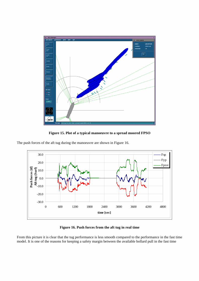
Figure 15. Plot of a typical manoeuvre to a spread moored FPSO The push forces of the aft tug during the manoeuvre are shown in Figure 16.

-30.0

-20.0

-10.0

0.0

10.0

20.0

30.0

0 600 1200 1800 2400 3000 3600 4200 4800

time [sec]

Push

forc

es [t

f] A

ft tu

g (S

urf)

FxpFypFptot

Figure 16. Push forces from the aft tug in real time From this picture it is clear that the tug performance is less smooth compared to the performance in the fast time model. It is one of the reasons for keeping a safety margin between the available bollard pull in the fast time

simulations and the bollard pull actually applied. It was also noticed that it is required to have a kind of electronic chart on the bridge combined with detailed information regarding speed (forward and lateral) and rate-of-turn. The limited objects within sight make it very difficult to judge the motion of the vessel and to take measures when required. From recently executed real time simulations it can be concluded that the fast time simulations give valuable results. In general operations controlled by a human being require more power than the operations controlled by the autopilot. On the other hand we saw that in specific emergency conditions the human being reacts more efficiently, thus reducing the probability of a collision. REFERENCES 1. Boom, H.J.J. van den, J.N. Dekker and R. P. Dallinga (1988), “Computer Analysis of Offshore Lift

Operations”, Offshore Technology Conference, Houston 2. Buchner, B. Van Dijk, A.W. and De Wilde, J.J. (2001). “Numerical Multiple-Body Simulations of Side-

by-Side Mooring to an FPSO”, ISOPE 2001, Stavanger 3. Cummins, WE (1962). "The Impulse Response Function and Ship Motions", DTMB Report 1661,

Washington D.C. 4. Feikema, G.J., R.H.M. Huijsmans and A. B. Aalbers (1992): “Low frequency motions of tankers on

tandem offloading conditions”, OTC paper # 6945 5. Huijsmans, RHM, Pinkster, JA and Wilde, JJ de (2001). “Diffraction and Radiation of Waves Around

Side-by-Side Moored Vessels”, ISOPE 2001, Stavanger 6. Oortmerssen, G van (1973): "The Motions of a Moored Ship in Waves", NSMB Publication No. 510 7. Oortmerssen, G van (1981): "Some Hydrodynamical Aspects of Multi-Body Systems", Int. Symposium

on Hydrodynamics in Ocean Engineering 8. Van Walree, F. and Willemsen, E. (1988). “Wind Load on Offshore Structures”, BOSS 9. Wichers, JEW (1987). “A Simulation Model for a Single Point Moored Tanker”, PhD thesis Delft

University of Technology 10. Wichers, J.E.W. and Van Dijk, A.W. (2000). “Investigation On F(P)SO Tandem Offloading Systems

Under Action Of Sudden Wind Squalls And Current Fluctuations”, 9th Offshore Symposium Texas Section of the SNAME, Houston