design and implementation of a computation server for ... · naval postgraduate school monterey,...

Calhoun: The NPS Institutional Archive

Theses and Dissertations Thesis Collection

2013-06

Design and implementation of a computation server

for optimization with application to the analysis of

critical infrastructure

Gun, Selcuk

Monterey, California: Naval Postgraduate School

http://hdl.handle.net/10945/34670

NAVALPOSTGRADUATE

SCHOOL

MONTEREY, CALIFORNIA

THESIS

DESIGN AND IMPLEMENTATION OF A COMPUTATIONSERVER FOR OPTIMIZATION WITH APPLICATION TO

THE ANALYSIS OF CRITICAL INFRASTRUCTURE

by

Selcuk Gun

June 2013

Thesis Co-Advisors: W. Matthew CarlyleThomas Otani

Second Reader: David L. Alderson

Approved for public release; distribution is unlimited

THIS PAGE INTENTIONALLY LEFT BLANK

REPORT DOCUMENTATION PAGE Form ApprovedOMB No. 0704–0188

The public reporting burden for this collection of information is estimated to average 1 hour per response, including the time for reviewing instructions, searching existing data sources,gathering and maintaining the data needed, and completing and reviewing the collection of information. Send comments regarding this burden estimate or any other aspect of this collectionof information, including suggestions for reducing this burden to Department of Defense, Washington Headquarters Services, Directorate for Information Operations and Reports (0704–0188),1215 Jefferson Davis Highway, Suite 1204, Arlington, VA 22202–4302. Respondents should be aware that notwithstanding any other provision of law, no person shall be subject to any penaltyfor failing to comply with a collection of information if it does not display a currently valid OMB control number. PLEASE DO NOT RETURN YOUR FORM TO THE ABOVEADDRESS.

1. REPORT DATE (DD–MM–YYYY)2. REPORT TYPE 3. DATES COVERED (From — To)

4. TITLE AND SUBTITLE 5a. CONTRACT NUMBER

5b. GRANT NUMBER

5c. PROGRAM ELEMENT NUMBER

5d. PROJECT NUMBER

5e. TASK NUMBER

5f. WORK UNIT NUMBER

6. AUTHOR(S)

7. PERFORMING ORGANIZATION NAME(S) AND ADDRESS(ES) 8. PERFORMING ORGANIZATION REPORTNUMBER

9. SPONSORING / MONITORING AGENCY NAME(S) AND ADDRESS(ES) 10. SPONSOR/MONITOR’S ACRONYM(S)

11. SPONSOR/MONITOR’S REPORTNUMBER(S)

12. DISTRIBUTION / AVAILABILITY STATEMENT

13. SUPPLEMENTARY NOTES

14. ABSTRACT

15. SUBJECT TERMS

16. SECURITY CLASSIFICATION OF:

a. REPORT b. ABSTRACT c. THIS PAGE

17. LIMITATION OFABSTRACT

18. NUMBEROFPAGES

19a. NAME OF RESPONSIBLE PERSON

19b. TELEPHONE NUMBER (include area code)

NSN 7540-01-280-5500 Standard Form 298 (Rev. 8–98)Prescribed by ANSI Std. Z39.18

20–6–2013 Master’s Thesis 2011-09-10—2013-06-21

DESIGN AND IMPLEMENTATION OF A COMPUTATION SERVERFOR OPTIMIZATION WITH APPLICATION TO THE ANALYSIS OFCRITICAL INFRASTRUCTURE

Selcuk Gun

Naval Postgraduate SchoolMonterey, CA 93943

None

Approved for public release; distribution is unlimited

The views expressed in this thesis are those of the author and do not reflect the official policy or position of the Department ofDefense or the U.S. Government. IRB Protocol number XXX.

Despite recent advances in the computational performance of decision support tools for Operations Analysis, there remains apersistent challenge in the deployment and use of sophisticated models by analysts who operate in limited computingenvironments. Recently, there has been a move toward cloud-based computing architectures that attempt to solve this problemby de-coupling the user interface from the remote computational resources. The objective of this thesis is to provide a flexibleand robust implementation of a server architecture and procedure for rapid development and deployment of decision supporttools. This thesis identifies functional requirements, develops an architecture to support those requirements, implements aprototype solution, and demonstrates the effectiveness of the solution for a simplified example of interdependent infrastructuresystems optimization.

Optimization, computation server, server architecture, critical infrastructure, interdependent infrastructures

Unclassified Unclassified Unclassified UU 107

i


ii

iii

Approved for public release;distribution is unlimited

DESIGN AND IMPLEMENTATION OF A COMPUTATION SERVER FOR

OPTIMIZATION WITH APPLICATION TO THE ANALYSIS OF CRITICAL

INFRASTRUCTURE

Selcuk Gun

First Lieutenant, Turkish Army

B.S., Turkish Military Academy, 2004

Submitted in partial fulfillment of the

requirements for the degrees of

MASTER OF SCIENCE IN SOFTWARE ENGINEERING

AND

MASTER OF SCIENCE IN OPERATIONS RESEARCH

from the

NAVAL POSTGRADUATE SCHOOL

June 2013

Author: Selcuk Gun

Approved by: Prof. W. Matthew Carlyle

Thesis Co-Advisor

Prof. Thomas Otani

Thesis Co-Advisor

Prof. David L. Alderson

Second Reader

Prof. Peter J. Denning

Chair, Department of Computer Science

Prof. Robert F. Dell

Chair, Department of Operations Research


iv

ABSTRACT

Despite recent advances in the computational performance of decision support tools for Opera-tions Analysis, there remains a persistent challenge in the deployment and use of sophisticatedmodels by analysts who operate in limited computing environments. Recently, there has beena move toward cloud-based computing architectures that attempt to solve this problem by de-coupling the user interface from the remote computational resources. The objective of thisthesis is to provide a flexible and robust implementation of a server architecture and proce-dure for rapid development and deployment of decision support tools. This thesis identifiesfunctional requirements, develops an architecture to support those requirements, implements aprototype solution, and demonstrates the effectiveness of the solution for a simplified exampleof interdependent infrastructure systems optimization.

v


vi

Table of Contents

1 Introduction 11.1 Current Practice in Optimization-Based Computational Decision Support . . . . 4

1.2 Objectives of This Thesis . . . . . . . . . . . . . . . . . . . . . . . 8

2 Requirements and Proposed Architecture 112.1 Usage Scenario . . . . . . . . . . . . . . . . . . . . . . . . . . . 11

2.2 Requirements . . . . . . . . . . . . . . . . . . . . . . . . . . . . 12

2.3 Proposed Architecture . . . . . . . . . . . . . . . . . . . . . . . . 15

3 The Implementation of the TALOS Computation Server 273.1 Server-Side Implementation . . . . . . . . . . . . . . . . . . . . . . 27

3.2 The Client-Side Implementation . . . . . . . . . . . . . . . . . . . . 33

4 The Analysis of Critical Infrastructure 374.1 Decoupled Infrastructure Models . . . . . . . . . . . . . . . . . . . . 38

4.2 The Optimization of DIMs Using The TALOS Computation Server . . . . . . 41

5 Conclusions and Future Work 575.1 Conclusions . . . . . . . . . . . . . . . . . . . . . . . . . . . . 57

5.2 Future Work . . . . . . . . . . . . . . . . . . . . . . . . . . . . 57

Appendices 59

A Server-Side Implementation Details 59A.1 agent Package . . . . . . . . . . . . . . . . . . . . . . . . . . . 59

vii

A.2 fileCtrl Package . . . . . . . . . . . . . . . . . . . . . . . . . . . 59

A.3 mdlPack Package . . . . . . . . . . . . . . . . . . . . . . . . . . 61

A.4 mdlUnpack Package . . . . . . . . . . . . . . . . . . . . . . . . . 62

A.5 mediator Package . . . . . . . . . . . . . . . . . . . . . . . . . . 62

B Client-Side Implementation Details 73B.1 dashBoard.html . . . . . . . . . . . . . . . . . . . . . . . . . . . 73

B.2 SGNet.js. . . . . . . . . . . . . . . . . . . . . . . . . . . . . . 73

B.3 csHandler.js . . . . . . . . . . . . . . . . . . . . . . . . . . . . 79

viii

List of Figures

Figure 1.1 Data Flow Diagram For Solving Optimization Models . . . . . . . . . 5

Figure 2.1 Preliminary Logical View of The TALOS Computation Server. . . . . 16

Figure 2.2 Mediator Connector. . . . . . . . . . . . . . . . . . . . . . . . . . . . 18

Figure 2.3 Logical View with Mediator Connectors. . . . . . . . . . . . . . . . . 19

Figure 2.4 Coupling values with and without mediator connector. . . . . . . . . . 20

Figure 2.5 Logical View of The TALOS Computation Server. . . . . . . . . . . . 22

Figure 2.6 Physical View of The Computation Server. . . . . . . . . . . . . . . . 23

Figure 2.7 Process View of The TALOS Computation Server. . . . . . . . . . . . 24

Figure 2.8 Scenario View of The TALOS Computation Server. . . . . . . . . . . 26

Figure 3.1 Development View of the TALOS Computation Server. . . . . . . . . 28

Figure 3.2 CNode Object Representing a Model With Its Input and Output Ele-ments. . . . . . . . . . . . . . . . . . . . . . . . . . . . . . . . . . . 35

Figure 4.1 Decoupled Infrastructure Model 1 and 2. . . . . . . . . . . . . . . . . 41

Figure 4.2 Decoupled Infrastructure Model 1. . . . . . . . . . . . . . . . . . . . 42

Figure 4.3 Decoupled Infrastructure Model 2. . . . . . . . . . . . . . . . . . . . 42

Figure 4.4 Total Penalty Values (vPenTotal) Required For DIM1. . . . . . . . . . 47

Figure 4.5 Both Dependent Arcs Off. . . . . . . . . . . . . . . . . . . . . . . . . 47

Figure 4.6 Only Arc r1n1pp− r1n2p Off. . . . . . . . . . . . . . . . . . . . . . 47

Figure 4.7 Only Arc r1n1pp− r1n3p Off. . . . . . . . . . . . . . . . . . . . . . 48

ix

Figure 4.8 Both Dependent Arcs On. . . . . . . . . . . . . . . . . . . . . . . . . 48

Figure 4.9 Net Cost v. Total Cost. . . . . . . . . . . . . . . . . . . . . . . . . . . 53

Figure 4.10 Total vPen Paid by DIM2. . . . . . . . . . . . . . . . . . . . . . . . . 53

Figure 4.11 DIM1 Objective Function Values. . . . . . . . . . . . . . . . . . . . . 53

Figure 4.12 DIM2 Objective Function Values. . . . . . . . . . . . . . . . . . . . . 53

Figure 4.13 Network Flow Until the 7th Cycle. . . . . . . . . . . . . . . . . . . . 53

Figure 4.14 Network Flow After the 7th Cycle and the 15th Cycle. . . . . . . . . . 54

Figure 4.15 Intermediate Network Flow Before the Redundancy Notification at the15th Cycle. . . . . . . . . . . . . . . . . . . . . . . . . . . . . . . . . 54

Figure B.1 The Web Interface For the TALOS Computation Server. . . . . . . . . 73

x

List of Tables

Table 4.1 Node Data For Decoupled Infrastructure 1. . . . . . . . . . . . . . . . 43

Table 4.2 Arc Data For Decoupled Infrastructure 1. . . . . . . . . . . . . . . . . 43

Table 4.3 Node Data For Decoupled Infrastructure 2. . . . . . . . . . . . . . . . 43

Table 4.4 Arc Data For Decoupled Infrastructure 2. . . . . . . . . . . . . . . . . 44

Table 4.5 Condition Table For Finding Redundancy. . . . . . . . . . . . . . . . . 50

xi


xii

Executive Summary

Optimization is one class of models used for decision support. This support is often in the formof suggesting a decision to minimize the costs or maximize the flow in a network. Solving anoptimization problem requires transforming the problem into a mathematical model and solvingthis model, often with the help of software-based computational tools.

Optimization is used in wide range of applications in business, government, and the military.More recently, optimization has been applied to problems related to the critical infrastructures.The critical infrastructures have vital functions in modern societies. Their disruption can havesignificant consequences.

Current practice in solving optimization problems suffers from various shortcomings. Someof these shortcomings are the lack of reusability, the difficulties in debugging, the absence ofmodular design, a general deficiency of visualization support, etc. When it comes to modelsrepresenting critical infrastructures, these deficiencies become more significant. Because criti-cal infrastructures do not exist in isolation, they depend on other infrastructures to maintain theirintended services. For instance, a natural gas infrastructure often needs electricity to power thepumps that move the gas through the pipe system. The electricity is provided by another criticalinfrastructure, the power grid which in turn also depends on other infrastructures to operate.The easiest way to model such a system of multiple critical infrastructures is often using a sin-gle but large model to be processed at once. This makes the already difficult tasks of designing,running, and debugging the models even more challenging. Moreover, solving real-world ap-plications often requires high computational power that an individual researcher or analyst canhardly provide.

In this thesis, we capture the requirements for a cloud-based computation server to support de-signing and running such models. We extend these requirements to include support for systemsof critical infrastructures.

In response to these requirements, we provide a flexible and robust architecture for a computa-tion server. Based on this architectural design, we implement the TALOS Computation Server.

We demonstrate the efficiency of using the TALOS Computation Server on a scenario consist-ing of two interdependent infrastructure models. In order to represent these infrastructures, wedesign stand-alone executable infrastructure models decomposed from a previous model of a

xiii

general purpose critical infrastructure system. These stand-alone infrastructure models are con-structed to have better control over the design, execution, and debugging stages of modeling asystem of critical infrastructures. We propose a two-stage optimization method that exploits theconveniences provided by the TALOS Computation Server. One of these conveniences is theTALOS Scripting Language that we created for designing a system of multiple models. TheTALOS Scripting Language is offered on a web-based terminal. We also provide a graphicaluser interface to perform the same tasks.

In addition to the support for the critical infrastructure models, the TALOS Computation Serveralso performs model integrity checking, meta-data generation, visualization of intermediate andfinal results, result reporting, and run-time error handling.

Our analysis of the mentioned scenario reveals that the TALOS Computation Server makes itmuch easier to design, run, and debug not only the single models but also the interdependentinfrastructure models compared to the previous solutions.

xiv

List of Acronyms and Abbreviations

API Application Programming Interface

DHS Department of Homeland Security

DIM Decoupled Infrastructure Model

GAMS Genaral Algebraic Modeling System

JSON JavaScript Object Notation

NEOS Network-Enabled Optimization System

RMI Remote Method Invocation

RPC Remote Procedure Call

VBA Visual Basic for Applications

VEGA Vulnerability of Electrical Power Grids Analysis

xv


xvi

Acknowledgements

I would like to express my very great appreciation to Professor Matthew Carlyle, ProfessorThomas Otani, and Professor David Alderson for their patient guidance, enthusiastic encour-agement, and constructive suggestions during the design and development of the TALOS Com-putation Server, and the analysis of critical infrastructures.

I would also like to extend my thanks to Meg Beresik for editing the thesis draft.

Finally, I’d like to thank my wife for her faithful support, continued understanding and encour-agement throughout my study.

xvii


xviii

CHAPTER 1:

Introduction

Decision-making in the 21st century is becoming increasingly challenging because of uncer-tainties, massive data sets, the need for real-time decisions, and the increased size and scope ofproblems. In the face of these challenges, the use of computational decision support tools canhave a significant impact on the quality of the decisions we make.

One class of models used for decision support is based on the mathematics of optimization. Op-

timization models use decision variables to represent problem choices and search for values thatmaximize or minimize objective functions of the decision variables. The decision variables aresubject to constraints on variable values expressing the limits on available sources or possibledecision choices (Rardin, 1998, p. 4-5).

Optimization is used in a wide range of applications to solve problems in business, governmentand the military. Some of these applications in different domains are:

• Scheduling Coast Guard district cutters (Brown et al., 1996),• Optimizing Army basing (Dell, 1998),• Optimizing military capital planning (Brown et al., 2004),• Reducing the fuel consumption of Navy ships (Brown et al., 2007),• Optimizing force positioning (Dell et al., 2008),• Solving the pallet loading problem (Martins and Dell, 2008), and• Optimizing assignment of Tomahawk Cruise Missiles (Newman et al., 2011).

More recently, optimization has been applied to problems related to critical infrastructures thatcan have a dramatic impact on society.

Modern societies depend on infrastructure systems (e.g. energy, communication, transportation)for vital functions, and their disruption can have significant consequences. For example,

in California, electric power disruptions in early 2001 affected oil and natural gasproduction, refinery operations, pipeline transport of gasoline and jet fuel withinCalifornia and to its neighboring states, and the movement of water from northernto central and southern regions of the state for crop irrigation. The disruptions also

1

idled key industries, led to billions of dollars of lost productivity, and stressed theentire Western power grid, causing far-reaching security and reliability concerns(Rinaldi et al., 2001).

The U.S. Department of Homeland Security (DHS) defines critical infrastructure as:

The assets, systems, and networks, whether physical or virtual, so vital to theUnited States that their incapacitation or destruction would have a debilitating effecton security, national economic security, public health or safety, or any combinationthereof. Key Resources are publicly or privately controlled resources essential tothe minimal operations of the economy and government (Department of HomelandSecurity, 2010, p. 46).

Critical infrastructures can be disrupted by two factors: natural events or adversary actions.Natural events such as an earthquake, flood, tornado, etc. occur at random and lend themselvesto probabilistic models.

However, adversaries do not act randomly but make deliberate decisions. This has led to thedevelopment of optimization-based models known as attacker-defender models.

An attacker-defender model is basically an optimization model of a system whose objectiverepresents the system’s value or cost while it operates. For instance, the maximum throughputof a pipeline network contributes to that system’s value, while power-generation costs, pluseconomic losses resulting from unmet demand, could represent the cost of operating an electricpower grid (Brown et al., 2006).

An attacker-defender model is based on the sequential actions of adversaries. First, we considera defender who operates the infrastructure with optimal configuration in terms of choosing howto route the flow over a network. An attacker, who is aware of this configuration, chooses theoptimal point of attack to cause the greatest damage with limited force. The defender respondsto this action by choosing the optimal configuration for the disrupted system.

The key assumption here is that the attacker has perfect knowledge of how the defender willoptimally operate his system, and the attacker will manipulate that system to his best advantage.This is equivalent to a strong but prudent assumption for the defender: He can suffer no worse ifthe attacker plans his attacks using a model different from that of the defender’s system (Brown

2

et al., 2005).

An attacker-defender model reveals what to protect among the components of a critical infras-tructure. Assuming limited resources to protect the infrastructure, this information is useful forprioritizing the strengthening efforts before any attack. The secondary output of this model is acontingency plan for the operator to maintain the services optimally after any attack.

Some applications of attacker-defender models include:

• The analysis of electricity grid security under terrorist threat (Salmeron et al., 2004,2009),• The D.C. subway system, improving airport security, and supply chains (Brown et al.,

2005),• The strategic petroleum reserve, border patrol, and electric power grids (Brown et al.,

2006),• The interdiction of a nuclear weapons project (Brown et al., 2009),• The tri-level optimization of western U.S. railroad resilience (Babick, 2009),• The optimization of port radar surveillance (Brown et al., 2011), and• Multi-modal delivery of coal (Alderson et al., 2012).

The domain-specific details of each application typically require customized models, outputreports, and visualization. For example, the Vulnerability of Electrical Power Grids Analy-sis (VEGA) identifies optimal or near-optimal attacks on electricity infrastructure and requiressophisticated visualization and animation of results to facilitate communication and understand-ing (Brown et al., 2005).

Despite the recent advances in computational performance of decision support tools for Opera-tions Analysis, there remains a persistent challenge in the deployment and use of sophisticatedmodels by analysts who operate in limited computing environments.

In real-world applications, optimization models can have thousands, even millions of variablesand constraints (Rardin, 1998, p. 4-5). In order to handle this complexity we use commerciallyavailable software systems known as solvers. We define the optimization model in a specializedoptimization language and run the solver via an interpreter to obtain a solution.

Among the problems we are facing, critical infrastructure analysis is one of the most demandingoptimization problems in terms of sophisticated modeling and necessary decision support tools.

3

One reason is the massive size of the infrastructure systems. For instance, the optimizationof large scale electric power grids in Salmeron et al. (2009) with large, real-world data setshas been unsolvable until the introduction of a global Bender’s decomposition algorithm. Thisalgorithm includes well defined process steps for solving the problem. The algorithm alsoincludes a cyclic sequence of model runs which is terminated using a termination gap.

Another reason that the study of infrastructure is difficult is because infrastructures do not ex-ist in isolation from one another. For instance, communication networks depend on electricity,transportation networks usually require computerized control and information systems, the gen-eration of electricity depends on fuels etc. (Rinaldi, 2004). We can define the interdependencyas a mutual relationship between two infrastructures through which the state of each infrastruc-ture affects or has correlation with the state of the other. We can say that two infrastructures areinterdependent when each has a dependency on the other (Rinaldi et al., 2001).

Understanding the nature of these interdependencies is essential to developing generalizablesolutions for the analysis of critical infrastructure.

1.1 Current Practice in Optimization-Based ComputationalDecision Support

The first step in solving any optimization problem is to transform the problem into a mathemati-cal model using a suitable notation. We use NPS Notation at Naval Postgraduate School (Brownand Dell, 2006). This notation facilitates communication and understanding among researchers.

Next, this mathematical representation is implemented in an optimization language. At NavalPostgraduate School we use the Genaral Algebraic Modeling System (GAMS) interpreter forsolving optimization problems. This interpreter comes with its own scripting language; GAMSLanguage for implementing models. This software is a commercial product bundled togetherwith the solvers. Depending on the type of optimization problem different solvers are selectedby default or user’s choice.

Running the model generates some output that needs to be perused and visualized depending onthe amount of data. The visualization of output is usually performed by transferring the outputdata to a statistical tool to generate some meaningful plots.

The data flows associated with the sequence of generating, running, and visualizing an opti-mization model are shown in Figure 1.1. Input files and parameters are used to define objective

4

function and constraints. The diagnostics report basically gives us information about the prob-lems encountered by the interpreter. Reports are the output files on which the interpreter writesthe solution information.

This straightforward sequence may be interrupted by a logical error in model, syntax error inscript, license expiration, or formatting error in input files. Multiple runs of a model usuallyrequire frequent manipulation of input files which might be tabular or textual.

Figure 1.1: Input elements for an optimization model are input data �les, parameters, and modelscript �le. These input elements are fed into a solver via the GAMS interpreter. Finally the GAMSinterpreter converts the output of the solver into output reports and diagnostic reports.

When solving complex optimization problems, an interface is very useful for facilitating dataentry, running multiple models sequentially, generating reports, and visualizing the results. De-ploying the solution with a user interface is also the preferred way when the problem needs tobe solved again and again with updated data and constraints by a non-expert user.

In the current environment, Microsoft Excel and its scripting language Visual Basic for Ap-plications (VBA) are often used for building a user-interface and automating the model runs.The choice of this application is based on the favorable learning curve of implementation withExcel/VBA and an assumed familiarity with the platform by most users.

However, this solution suffers from some serious shortcomings:

• Local computation: Obtaining a solution relies on the existence of licensed GAMS and

5

solvers on each system. This means each user needs a computer for heavy-weight com-putation during model runs which may sometimes take hours or days.• Platform dependency: Excel/VBA runs on Microsoft Windows operating systems and

sometimes demonstrates non-standard behavior on the Apple Mac OS. Applying this so-lution on open-source operating systems requires purchasing necessary licenses and usingvirtual machine.• Lack of reusability: Data entry and visualization are dependent on the implementation of

the model. It is typically not possible to reuse the interface for another model.• Monolithic Models: Complex models of system operation often require an understanding

of one or more subsystems. In the current computing environment, it is often the easiestto implement all submodels in a single GAMS file. This type of monolithic model isconceptually straightforward but can be very complicated. Because it requires the analystto understand all the details of every submodel this type of implementation can becomeuntenable for large systems. While using a monolithic model, it is hard to debug the scriptand see the intermediate results which might be an early warning of a mistake or success.• Lack of debugging: Due to the limitations of the programming environment it is hard to

detect the faults and repair them.• No repository for models: This solution does not offer any tagging for models since it is

intended for a specific problem. It is infeasible to build a repository of solutions owing tothe non-standard approaches adopted.• No access control: This solution does not keep track of the people modifying the data,

and their modification. The generated reports may not be the result of the original inputdata.

In addition to these shortcomings, the optimization has some inherent difficulties. Optimizationlanguages are not general purpose languages, so we usually do not expect much flexibilityfrom the language and support from a user community. Collaboration options such as versioncontrol systems, user forums, open-sourcing of the model scripts and bug tracking are almostcompletely ignored while using these languages.

Moreover, the optimization model resides in the researcher’s hard drive in a script file bundledwith a number of input and output files. Accessing these implementations usually require con-tacting the author of an article and requesting the script. The difficulty in finding the modelamong many others depends on the author’s arrangement on his hard drive. Trying to under-stand a researcher’s implementation is often challenging due to the lack of documentation.

6

Depending on the performance of the algorithms and solvers used, and the scale of the problem,the execution time of a model can change from a few milliseconds to hours. Considering theoverhead of running these models on personal computers in terms of software acquisition cost,execution time, and installation troubles, recently there has been a move toward "cloud-based"computing architectures that attempt to solve this problem by decoupling the user interface fromthe remote resources. Computation servers are the physical elements responsible for minimiz-ing this overhead on the platform.

There are various projects to move the solvers and interpreters to the cloud. Among theseprojects, the Network-Enabled Optimization System (NEOS) provides the most advanced facil-ities to its users. Dolan et al. (2008) describe the NEOS server as the most ambitious realizationof the optimization server concept. "Operated by the Optimization Technology Center of Ar-gonne National Laboratory and Northwestern University, it represents a collaborative effortinvolving over 40 designers, developers, and administrators around the world" (Dolan et al.,2008). The NEOS server provides a high level of flexibility to its users in choosing the op-timization language. Using the translators located on the server-side the server translates thegiven script into the format that is specifically needed for the chosen solver.

The apparent motivation of the designers of the NEOS server looks to be serving a large numberof users using a wide range of optimization languages. As a result of this endeavor they havemanaged to gather data sets containing valuable information about user and model profiles interms of problem type, solver type, and optimization language ranges of execution time fordifferent classes of problems. The experience gathered with the NEOS server is very significantconsidering the monthly average number of submissions to the NEOS Server which is more than40,000 since 1996. The NEOS Server also provides the Application Programming Interface(API) to submit jobs and receive results using XML-RPC (XML formatted file based remoteprocedure call). This API is compatible with various languages such as C/C++, Java, Python,Perl, PHP and Ruby, etc.

The NEOS server and similar projects help users by providing remote computation power andfree access to granted solvers. Unfortunately the needs associated with error handling, visual-ization, storing the models with well-defined tags, collaboration tools, and support for designinginterdependencies among models are not addressed in present solutions.

As expressed in Rinaldi (2004), modeling and simulating infrastructure interdependencies arefar from easy exercises. Developing appropriate tools is technically challenging, with numerous

7

hurdles to overcome (Rinaldi, 2004). Making use of the foundations software engineering andoperations research, it is possible to design and implement a computation server that providessupport for building and running interdependent infrastructures.

1.2 Objectives of This ThesisIn this thesis we identify the functional requirements for a cloud-based computation serverand present a design and implementation of a computation server that may run any model scriptwritten in GAMS on the cloud. Our design is intended to facilitate the analysis of interdependentcritical infrastructure systems. We have tried to provide the useful capabilities that a researcherwould expect from a computation server in terms of optimization. Some of these features are:

• Model integrity checking: Every model uploaded to the system is parsed to find its depen-dent input and expected output files. The user is notified to complete any missing itemprior to model runs.• Meta-data generation: The server automatically generates meta-data which will be useful

for storing and searching the models in a repository.• Visualization: Line, bar and pie charts are supplemented with our network graph imple-

mentation to visualize intermediate and final results.• Reporting: Users will be able receive continuous progress information together with user-

defined output files.• Error Handling: Errors arising from GAMS implementation are displayed in a user-

friendly way for easy debugging• Graphical user interface: A web browser is the only software needed for accessing the

server and designing and running the models.• Scripting on terminal: A terminal embedded on the web interface accepts the commands

written in a customized scripting language that we have developed.• Super-system design: The user may design and run a super-system which represents in-

terdependent infrastructures either using command line instructions on terminal or web-interface. This capability allows the users to define sequential and even cyclic model runstogether with automated data manipulation.

To our knowledge, this is the first time that a computation server has provided support forcritical infrastructure analysis together with other tools to facilitate optimization-based decisionmaking. In this thesis we also demonstrate the effectiveness of the solution for interdependentinfrastructures which are the basis for critical infrastructure analysis.

8

Ultimately, this solution works if it supports all previous models implemented in GAMS. Theefficiency of the support provided for critical infrastructure analysis will depend on the level atwhich the monolithic models are decomposed into modular units.

The primary contribution of this thesis is providing a standardization of optimization modelsso that the models can be stored, searched, run, and understood easily, showing the efficiencyof using well-designed decision support tools on optimization, especially on the challenginganalysis of critical infrastructures.

In what follows, we explain the requirements and architecture of the TALOS ComputationServer we have implemented in Chapter 2. We provide the implementation details in Chapter3, and finally we demonstrate the analysis of interdependent infrastructures using the TALOSComputation Server and discuss the effectiveness of using our solution in Chapter 4. We con-clude with a summary and discussion of future work in Chapter 5.

9


10

CHAPTER 2:

Requirements and Proposed Architecture

In this chapter, we perform requirements analysis in order to capture the expectations of theusers. Based on these requirements, we define the TALOS Computation Server and classify theusers of the TALOS Computation Server. And finally, we propose an architectural design usingthe 4+1 view model.

2.1 Usage ScenarioAlthough there are many potential users of a computation server, we limit our attention to opera-tions research students and faculty using optimization in their research at the Naval PostgraduateSchool.

These users have different levels of familiarity with optimization methods and optimizationlanguages. Moreover, their expectations for a computation server can differ greatly. For in-stance, model integrity checking, run-time error checking, and graphical user interfaces arevalued by students, while the ability to conduct multiple model runs, data file manipulation, anda command-line interface are valued by faculty researchers working in the field of optimization.

Considering these differences in the level of familiarity and expectations, we classify users intwo groups:

• Basic users: The users with minimum or average familiarity with optimization and theGAMS language, mostly running single optimization models with small problem scope;• Advanced users: The users with advanced knowledge or familiarity with optimization

and the GAMS language, running both single and multiple optimization models rangingfrom small scale to large scale (real world) problems.

For both groups of users, the basic interaction with the TALOS Computation Server consists oftwo parts. First, the user loads the model on to the server. To do this, the user logs in to theserver with provided credentials and uploads the files that form an optimization model using aweb interface. The server locates the main script file among the received files and parses this fileto detect the input files needed for running the model. If any missing file is detected, the user isnotified about the missing file. The user is expected to complete the necessary input files. TheTALOS Computation Server automatically generates meta-data which includes the user name,

11

date and time, input and output files. Moreover, the TALOS Computation Server creates anarchive including the meta-data and model files. The user may download this archive from therepository maintained by the server. The next step for the basic users is to run the model.

Advanced users may prefer uploading multiple models by repeating the previous steps. In orderto run multiple models, the user must specify a run sequence. We call the run sequence asuper-system design. The user can design the super-system making use of the web interfaceor command line interface. A super-system design allows the user to define global variablesto keep track of model parameters and data flow to perform interaction between models. Aftercompleting the super-system design, the user runs the super-system.

The second part of using the TALOS Computation Server involves executing the model. The runrequest is queued by the TALOS Computation Server. The user may prefer getting the resultslater or monitoring the progress immediately. The basic user running a single model receivesthe optimization results or error messages translated by the TALOS Computation Server. Theadvanced user requesting a multiple-model run receives intermediate results for model runs andmonitors how the super-system run is progressing by looking at the interactive plots and results.This allows the advanced user to pause the system before running a model in the sequence, tomodify the super-system, and to resume the super-system run.

2.2 RequirementsAn important step in the software development life cycle is to capture and analyze the concernsand the needs of the potential users. Traditionally these requirements are classified in twogroups:

• Functional requirements: The expected behaviors and particular results from the systemthat is being designed.• Non-functional requirements: Non-behavioral features mostly referring to the evolution

of the system such as maintainability, scalability, etc.

There are various methods for documenting the requirements. We describe the requirements ina goal hierarchy as in Berzins and Luqi (1991, p. 154). The following subsections summarizethe expectations from the TALOS Computation Server, making use of the goal hierarchies forfunctional and non-functional requirements. The architectural design and implementation areperformed in accordance with these requirements.

12

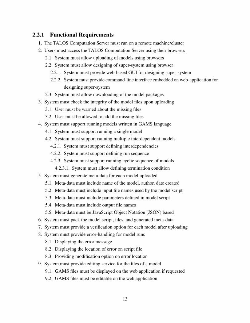
2.2.1 Functional Requirements1. The TALOS Computation Server must run on a remote machine/cluster2. Users must access the TALOS Computation Server using their browsers

2.1. System must allow uploading of models using browsers2.2. System must allow designing of super-system using browser

2.2.1. System must provide web-based GUI for designing super-system2.2.2. System must provide command-line interface embedded on web-application for

designing super-system

2.3. System must allow downloading of the model packages

3. System must check the integrity of the model files upon uploading

3.1. User must be warned about the missing files3.2. User must be allowed to add the missing files

4. System must support running models written in GAMS language

4.1. System must support running a single model4.2. System must support running multiple interdependent models

4.2.1. System must support defining interdependencies4.2.2. System must support defining run sequence4.2.3. System must support running cyclic sequence of models

4.2.3.1. System must allow defining termination condition

5. System must generate meta-data for each model uploaded

5.1. Meta-data must include name of the model, author, date created5.2. Meta-data must include input file names used by the model script5.3. Meta-data must include parameters defined in model script5.4. Meta-data must include output file names5.5. Meta-data must be JavaScript Object Notation (JSON) based

6. System must pack the model script, files, and generated meta-data7. System must provide a verification option for each model after uploading8. System must provide error-handling for model runs

8.1. Displaying the error message8.2. Displaying the location of error on script file8.3. Providing modification option on error location

9. System must provide editing service for the files of a model

9.1. GAMS files must be displayed on the web application if requested9.2. GAMS files must be editable on the web application

13

9.3. Data files (.csv) must be displayed in a table on web application if requested

10. Progress must be displayed

10.1. User must be notified about which model is being run10.2. User must be able to see the intermediate results (for multiple model runs)

11. User must be given control over the model runs

11.1. User must be able to pause the model runs11.2. User must be able to terminate the model runs11.3. User must be able to reset the model runs11.4. User must be able to rewind any sequence of runs

12. Results must be displayed

12.1. Results must be displayed numerically12.2. Results must be visualized

12.2.1. User must be able to see Network Problem results on Network Graph12.2.2. User must be able to see the other results on line plots

12.2.2.1. Tabular output files must be displayed if requested12.2.2.2. Optimal Values of a Model that was run multiple times must be displayed

if requested

13. User must be notified about the end of model runs

13.1. User must be notified via e-mail if non-interactive mode is selected13.2. User must be notified via animations if interactive mode is selected13.3. Intermediate results must be kept for only interactive mode

2.2.2 Non-Functional Requirements1. System must be secure

1.1. Access control must be applied for each user1.2. User inputs must be validated

2. System must be scalable

2.1. System must be responsive for a maximum of 100 users accessing the server

2.1.1. Queuing must be based on FIFO (first-in first-out) protocol

2.2. System must be making use of Torque Resource Manager for Cluster Computing2.3. System must be adaptable to any other resource manager

3. System must be maintainable

3.1. System must be dependent on one COTS (commercial off-the shelf): GAMS&Solvers3.2. Non-stable libraries must be avoided

14

3.3. Comprehensive documentation must be prepared and updated with every build

2.3 Proposed ArchitectureThe architecture of a software system refers to the set of principal design decisions in accor-dance with the requirements for this system. The most convenient way of designing and explain-ing the architecture of a software system is using view diagrams. These view diagrams includemostly the components as the building blocks of the architecture and the connectors whichstand for the interaction services among the components. Connectors are primarily responsiblefor the abstraction and the separation of concerns while providing interaction services betweencomponents and/or connectors in software architecture (Taylor et al., 2009). Traditionally, theinteractions between the connectors and/or components have been in the form of function calls,association classes, class inheritance and shared memory.

The TALOS Computation Server we develop in this thesis is a distributed software system thatprovides tool sets for optimization services to the analysts, scientists, and decision makers.

A distributed system is a system consisting of several computers that communicate through anetwork that uses a common set of distributed protocols to provide the coherent execution ofdistributed activities (Amirat and Oussalah, 2009).

To satisfy the requirements presented in section 2.2, we propose the architecture shown in Fig-ure 2.1. The architectural design is presented at a high level to highlight the interactions betweenthe distributed components clearly.

The components in the proposed architecture are the Browser, Apache Server, Agent, DatabaseServer, Computation Server, and GAMS & Solver Modules. The main challenge in the archi-tecture is to provide content-rich services in primal connectors.

In describing the connectors in the proposed architecture, we use the connector types presentedin Taylor et al. (2009, p.164). There are eight connector types. Four of them are relevant in thisthesis:

• Procedure call: Performs data transfer among interacting components using the parame-ters and return values,• Event: In this connector type, the flow of control is initiated by an event. Event connector

notifies all interested parties about the event by sending them messages and passing the

15

Figure 2.1: Preliminary Logical View of The TALOS Computation Server.

control.• Data Access: This connector prepares data, allows other components to access data and

finally performs clean-up.• Stream: Stream connectors facilitate data flow between autonomous processes via Unix

pipes, TCP/UDP communication sockets, etc.

We often use these connectors together in the form of composite connectors.

The interactions among different pairings of components are as follows:

Browser - Apache Server: Interaction services include uploading/downloading (stream and dataaccess) operations, notifying ready state (event), and delivering result (distributor). We use acomposite connector here. Event-based data distribution connector is appropriate for facilitatingthe interaction services.

Apache Server-Agent: The Apache Server being a commercial off-the shelf (COTS), as such,the interaction service is implemented with a stream connector.

Agent – Computation Server: These components share the following interaction services: Jobrequest (procedure call), query results (data access), get/send results (stream), provide access

16

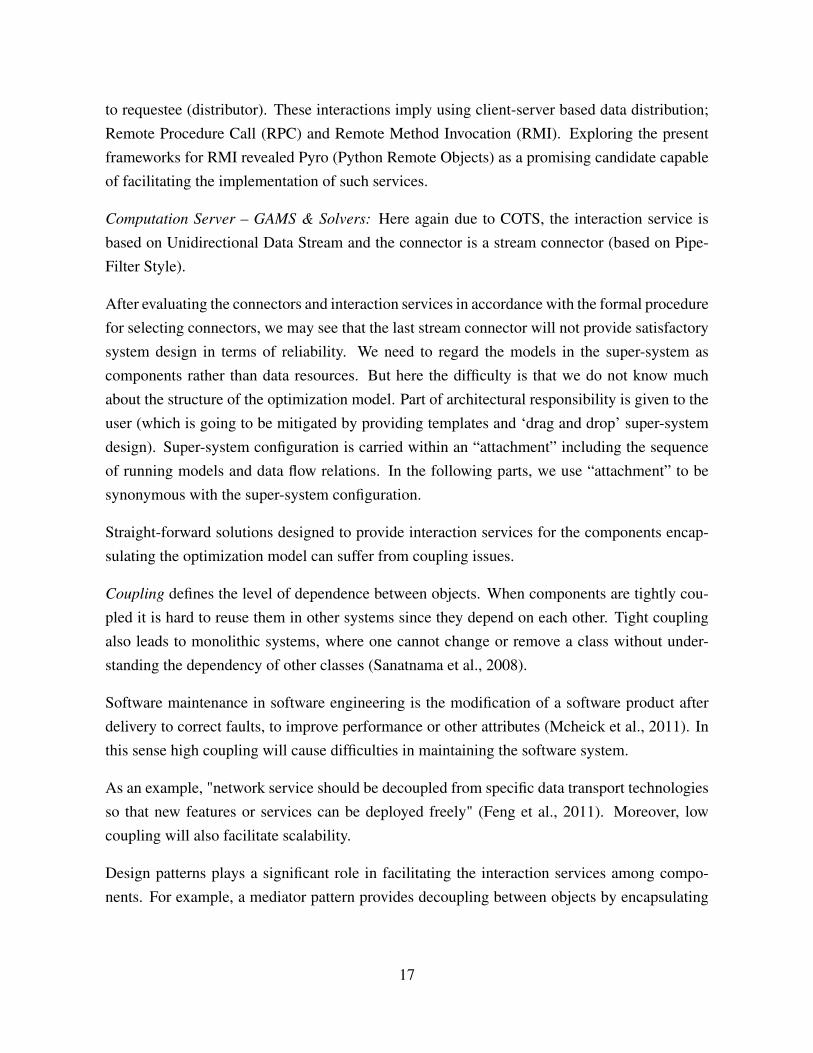
to requestee (distributor). These interactions imply using client-server based data distribution;Remote Procedure Call (RPC) and Remote Method Invocation (RMI). Exploring the presentframeworks for RMI revealed Pyro (Python Remote Objects) as a promising candidate capableof facilitating the implementation of such services.

Computation Server – GAMS & Solvers: Here again due to COTS, the interaction service isbased on Unidirectional Data Stream and the connector is a stream connector (based on Pipe-Filter Style).

After evaluating the connectors and interaction services in accordance with the formal procedurefor selecting connectors, we may see that the last stream connector will not provide satisfactorysystem design in terms of reliability. We need to regard the models in the super-system ascomponents rather than data resources. But here the difficulty is that we do not know muchabout the structure of the optimization model. Part of architectural responsibility is given to theuser (which is going to be mitigated by providing templates and ‘drag and drop’ super-systemdesign). Super-system configuration is carried within an “attachment” including the sequenceof running models and data flow relations. In the following parts, we use “attachment” to besynonymous with the super-system configuration.

Straight-forward solutions designed to provide interaction services for the components encap-sulating the optimization model can suffer from coupling issues.

Coupling defines the level of dependence between objects. When components are tightly cou-pled it is hard to reuse them in other systems since they depend on each other. Tight couplingalso leads to monolithic systems, where one cannot change or remove a class without under-standing the dependency of other classes (Sanatnama et al., 2008).

Software maintenance in software engineering is the modification of a software product afterdelivery to correct faults, to improve performance or other attributes (Mcheick et al., 2011). Inthis sense high coupling will cause difficulties in maintaining the software system.

As an example, "network service should be decoupled from specific data transport technologiesso that new features or services can be deployed freely" (Feng et al., 2011). Moreover, lowcoupling will also facilitate scalability.

Design patterns plays a significant role in facilitating the interaction services among compo-nents. For example, a mediator pattern provides decoupling between objects by encapsulating

17

the communication between components with a mediator object. With the mediator pattern, ob-jects do not communicate directly with each other any more, instead they communicate throughthe mediator. This reduces the dependencies between communicating objects, thus, reducingthe coupling. However, keeping the components as the origin of control still leads to tightcoupling (Sanatnama et al., 2008).

As a solution to address the challenge posed by dynamic model interaction services, we haveused mediator connectors inspired by the mediator pattern.

Mediator connector parses the attachment file and builds up the system by initiating all thecomponents and the connections (method calls) described in each interaction. The sequence ofmethod invocations in the form of interactions can be performed by invoking the run method inthe mediator connector using the name of interaction as an input parameter (Sanatnama et al.,2008).

Figure 2.2: Mediator Connector.

The attachment is also used to generate the wrappers around the dynamic optimization mod-els. These components, connectors and wrappers, are not directly instantiated by the mediatorconnector; they are generated using the factory pattern.

18

One immediate advantage of automatic connector construction at runtime is the reduction inhuman intervention (Pahl and Yaoling Zhu1, 2009).

In this design, components (optimization model and wrapper) are not allowed to interact directlywith the other components. Such a design will make interception of faults and handling faultsmore practical. A more traditional way would rely on reading the script file and then loggingthe failure.

Moreover, a mediator connector provides low coupling among the components. The integrationof the mediator connector in the preliminary logical view is shown in Figure 2.3.

Figure 2.3: Logical View with Mediator Connectors.

In order to measure the coupling between components, the Coupling Between Objects (CBO)metric, developed by Chidamber and Kemerer, can be used. We can say that two componentsare coupled if and only if at least one of them acts upon the other. In other words, since couplingis the degree of interaction between classes, the basic idea underlying all coupling metrics is thenumber of interclass interactions in the system. Multiple accesses to the same class are countedonly once (Sanatnama et al., 2008). Consider the case where five optimization models are to

19

be run within a loop; we can observe the difference in CBO values between using the mediatorconnector and not using it in Figure 2.4.

Figure 2.4: Coupling values with and without mediator connector.

So far we have focused on the non-functional properties such as reliability, scalability, andmaintainability. There is usually a trade-off between performance and maintainability in soft-ware architecture. Generating connectors and wrappers on the fly can decrease the performanceof the system, but this is justifiable considering the different language (GAMS language) in theoptimization model and the presence of COTS software (GAMS&Solver). Performance con-cerns are prevalent in a design encompassing all native components as in Pahl and Yaoling Zhu1(2009) and Sanatnama et al. (2008).

To provide more details of our architecture, we present our design using the ‘4+1 view model’(Kruchten, 1995). It consists of four main views each of which represents a different perspectiveof stakeholders, and a complementary view as follows:

• Logical view,• Process view,• Physical view,• Development view, and• Scenarios.

20

2.3.1 Logical ViewA logical view demonstrates the object model of the design. We have decomposed the systeminto a set of key abstractions which primarily support the functional requirements. As a guide-line we have tried to maintain a single and coherent object model across the system and avoidpremature specialization of classes as suggested in Kruchten (1995).

We have shown that the expected behaviors from the TALOS Computation Server can be ad-dressed using the three main class groups shown in Figure 2.5. These class groups are:

• Agent: Agent is responsible for responding to the queries sent by the users.• Utility Packages: This group includes the utilities shared by other groups. These utilities

are given below:– fileCtrl: This module is responsible for checking the integrity of model files. Any

missing file among the model files is detected by this module.– mdlPck: This module is responsible for generating the meta-data and packing the

files with generated meta-data.– mdlUnpack: Extraction of the model packages is performed by this model.

• Computation server daemon and utilities: The daemon is responsible for respondingto the agent requests, running the models, and performing the tasks defined in the super-system configuration (attachment file) using its numerous utility classes.

2.3.2 Physical ViewThe physical view serves as a mapping from the software to the hardware.

In order to address the non-functional requirements such as maintainability and scalability,GAMS and solvers must be detached from the TALOS Computation Server machine. The moti-vation is to consider the future need for more CPU power with the increasing number of clients.In this way, making a seamless transition to a cluster of workers will be possible. This allowsus to run the machine executing the GAMS and solvers very close to its maximum processorload while giving the daemon machine less load in order to decrease response time.

A physical view of the TALOS Computation Server is given in Figure 2.6. Users connect to theTALOS Computation Server from numerous machines and then communicate with the Apacheserver located in the daemon machine. Similarly, each of the GAMS and solver machinescommunicates with a resource manager located in daemon machine. In order to increase thecapacity of the TALOS Computation Server, adding more machines with GAMS and solvers

21

Figure 2.5: Logical View of The TALOS Computation Server.

installed is sufficient. The physical view of the TALOS Computation Server also representsthe level of freedom to manipulate the internal structure of each entity with black, grey orwhite colors. Entities shown in black give us no chance to interfere with the internal structurewhile the grey one (resource manager) provides us with limited options to manipulate internalbehavior.

2.3.3 Process ViewSome of the non-functional requirements such as performance and availability are taken intoaccount by the process view. Concurrency and distribution are also addressed by the processview (Kruchten, 1995).

Concurrency is one of the critical issues to maintain the services expected from the TALOSComputation Server. Maintaining a responsive system requires making use of multi-processingor multi-threading. We can define the process as a set of instructions that form an executableunit. We define thread as a lightweight process.

We identify the processes that require concurrency in the TALOS Computation Server architec-ture making use of the process view shown in Figure 2.7. The Agent process is initiated by theuser or the daemon on demand as a short-lived process which terminates upon completing its task.

22

Figure 2.6: Physical View of The Computation Server.

The daemon process is an infinitely running process as its name suggests. Inside the daemonprocess we have designed listener and attachment instances which are initiated by the daemon.Listener and attachment instances are long-lived separate threads. The rationale for designingsuch threads is the need for communicating with the TALOS Computation Server while it is run-ning a super-system. This communication can be about instant information about the progress,pause request, terminate request sent by the user, or run-time error in the model script.

2.3.4 Development ViewWe have demonstrated the actual software module organization in the software developmentenvironment using the development view. This view reveals all the subsystems of the softwareand gives an idea about the planning and time allocation for each subsystem.

We have partitioned the object model of the design given in the logical view to include everysingle class and data structure to facilitate implementation. Before implementation it is verydifficult to define all software elements but it is possible to list the rules that provides guidanceto software development. The development view is given and explained in Chapter 3.

23

Figure 2.7: Process View of The TALOS Computation Server.

2.3.5 ScenariosScenarios form the additional view in the ‘4+1 view model’. We may consider scenarios asthe abstraction of requirements that complements the other views. Using scenarios facilitatesdiscovering the architectural elements, validating and illustrating the architectural design. Sce-narios are a small set of use cases based on general use cases (Kruchten, 1995).

We have defined a general use case shown in Figure 2.8. The user in this scenario is assumed tobe an advanced user. The scenario is as follows:

1. User logs into his account using browser or mobile application.2. User selects uploading a model.3. Server-side ‘Agent’ detects the .gms file and associated files in the remote directory that

is allocated to the user.4. If all of the files are present, the files are accepted by the server and packed to form a

model file on the server. If there is any missing file, the user is notified to provide missingfiles.

5. If ‘verify’ is selected by the user, ‘Agent’ runs the packed model using the GAMS andverifies expected results are generated. If verification reveals errors in the model script,error text is parsed to return a notification to the user. Verification is only performed formodels with short-duration (Agent is also responsible for terminating blocked processes).

6. If there are any other models to upload, steps 2 to 5 are repeated.7. User designs a super-system and submits to the server;

24

(a) Run sequences (steps) are specified as from model A to model B (in order to runmodel B after A).

(b) For each run step data file/parameter modifications and interactions are defined.(c) Two previous steps are repeated until a desired super-system is generated.

8. User selects “Run super-system”,9. Agent adds the request to the queue,

10. The TALOS Computation Server initiates the processes defined in the first super-systemfile at the top of the queue. The server will be always running and grabbing the requestfrom the queue as long as it is idle. Agent runs on demand sent by user.

11. The TALOS Computation Server provides information about the progress of the processes(model runs, present cycle numbers, etc).

12. Agent sends the results to the client via Apache Server.13. Results are displayed in client’s web-GUI.

Using the scenario view in Figure 2.8 we can follow the sequence of interaction between theprocesses.

Subsets of this general use case can include one or more of the following actions:

• Updating one or more models,• Changing the initial parameters of the model(s),• Changing the termination conditions,• Creating another super-system,• Rerunning the model with above updates.

The investment in requirements analysis and architectural design with the application of 4+1view model pays back during the rest of software development life cycle. In accordance withour requirements analysis and architectural design, we explain the details of the TALOS Com-putation Server implementation in Chapter 3.

25

Figure 2.8: Scenario View of The TALOS Computation Server.

26

CHAPTER 3:

The Implementation of the TALOS Computation Server

The TALOS Computation Server is implemented to run on Unix based operating systems ca-pable of running Python 2.x and Apache Server. We have designed the TALOS ComputationServer to be accessed via a web browser. In this sense, our implementation is divided intoserver side and client side to achieve a client-server architectural design pattern. The devel-opment view of the TALOS Computation Server is shown in Figure 3.1. This view basicallyreveals the implementation details of the components introduced in Chapter 2.

3.1 Server-Side ImplementationThe core tasks of the TALOS Computation Server are authentication, request queuing, modelverification, upload/download, super-system creation, and interaction with GAMS solvers. Thesetasks are implemented by the following Python packages:

• agent,• fileCtrl,• mdlPack,• mdlUnpack, and• mediator.

These packages are implemented in an object-oriented manner. Each package is composedof several classes. A detailed description of the packages and their elements is given in theremainder of the section.

3.1.1 The agent PackageThis package contains the functions that facilitate the communication between the Apacheserver and the TALOS Computation Server. The agent is called automatically when the useraccesses the TALOS Computation Server, generates or modifies a super-system, sends a runrequest to the TALOS Computation Server. If the user chooses to see the progress of the super-system run, the agent will publish feedback on the progress back to the user. During the feed-back, the user will have an option to interrupt the running sequence and modify the GAMSscript or input files.

27

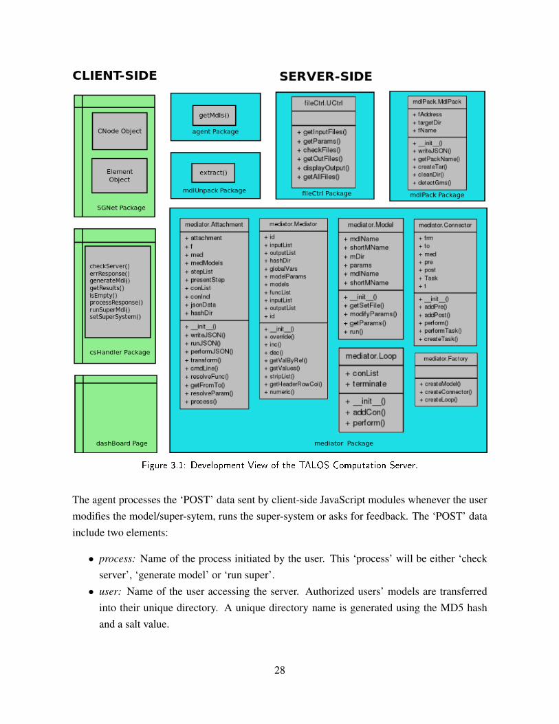
Figure 3.1: Development View of the TALOS Computation Server.

The agent processes the ‘POST’ data sent by client-side JavaScript modules whenever the usermodifies the model/super-sytem, runs the super-system or asks for feedback. The ‘POST’ datainclude two elements:

• process: Name of the process initiated by the user. This ‘process’ will be either ‘checkserver’, ‘generate model’ or ‘run super’.• user: Name of the user accessing the server. Authorized users’ models are transferred

into their unique directory. A unique directory name is generated using the MD5 hashand a salt value.

28

The agent package contains a helper function getMdls which is responsible for fetching theautomatically generated meta-data during the ‘generate model’ process. The content of eachmodel’s meta-data is used to generate a graphical representation of each model in the web GUI(client side).

The agent accepts the following process requests:

• ‘check server’ Process: In this process the agent checks for a valid model in the unique(hashed) directory provided to the user using getMdls function.• ‘generate model’ Process: This process is initiated automatically after every model is

uploaded to the server. When the user uploads a model script and input files, they aretransferred into a temporary upload directory of the user. Integrity checking of the modelscript, meta-data generation and packing tasks are performed by making use of the func-tionalities provided by fileCtrl and mdlPack packages in this process. Finally, the tempo-rary upload directory is cleaned for new uploads.• ‘run super’ Process: This process is initiated when the user completes the design of

a super-system. The agent requires another post data element ‘stepList’ which containsthe super-system design data in order to start this process. Super-system design datais generated on the client by transforming the users’ graphical design or command-lineinstructions into JSON data. The super-system is run making use of the handlers providedby mediator package in this process.

3.1.2 The fileCtrl PackageThis package contains the UCtrl class with its member functions for getting input files, param-eters, and output files and for checking file integrity. Member functions implemented in theUCtrl class are given in Appendix A.

3.1.3 The mdlPack PackageThis package contains the MdlPack class with its member functions for detecting GAMS filesin a given directory, generating meta-data and packing the model files.

The mdlPack package also extracts the model script filename using the provided arguments. Ifno filename is provided, the package detects the GAMS script file in the given directory usingdetectGms function.

Member functions implemented in the MdlPack class are given in Appendix A.

29

3.1.4 The mdlUnpack PackageThis package contains the functionality for extracting the model files from the archive. Memberfunctions implemented in this package are shown in Appendix A.

3.1.5 The mediator PackageThis package contains the core functionality of the TALOS Computation Server. Instead oftreating the super-system design file as a set of instructions to be performed line by line andforgetting the previous processed lines, the mediator package provides an encapsulation mecha-nism over the model script, pretasks and posttasks. Pretasks and posttasks are the tasks used forperforming the data flow between models and assignments to the user-defined variables. In thisway, each model run is named as step that is state-aware. Stateful steps facilitate implement-ing a feedback mechanism to understand the current state of multiple model runs. Data flowbetween models is achieved by overriding input files with new values, another models’ outputfiles, or the partition of a file. These mechanisms are implemented in the following classes:

The Mediator ClassThis class creates components (models) and connectors using the attachment. There will be onemediator instance for each super-system created. This instance stays alive until the super-systemis solved and the user is satisfied with the results.

The Mediator is the main controller of all other classes in this package.

When the Mediator class is initialized, global dictionaries and lists are created for all modelsthe user has uploaded previously. These dictionaries and lists are:

• Model Dictionary: This dictionary is populated with mappings from model name tomodel object generated using the Factory class.• Variables Dictionary: The TALOS Computation Server captures the objective function

value of each model by default. This value is represented as “modelName$Z” where theprefix before the dollar sign represents the model name. By default “modelName$Z”maps to an empty list. This list is appended with new objective function value after eachrun of a model.The user may define a new global variable during super-system design to facilitate inter-actions between models.• Model Parameters Dictionary: This dictionary is populated with single-value (scalar)

parameters and multi-dimensional parameters. Parameter names, in the form of “mod-

30

elName$paramA”, are mapped to user-defined values in order to run the model with aspecific parameter.• Function Dictionary: The TALOS Computation Server provides several commands, such

as inc, dec, and override, to facilitate bindings between models. These commands aremapped into the object address of their associated functions. While the override functionis used for almost every pretask or posttask, the other functions are expected be moreuseful while running some models in a loop.• Input List: This list is populated with the input filenames generated by the fileCtrl Pack-

age. If the user prefers to use the command-line interface this list is used to verify thatthe files associated in pretask or posttask are valid.• Output List: This list is populated with the output file names generated by the fileCtrl

Package. Similarly this list is used to verify the model bindings while defining pretask orposttask on the command-line interface.

Member functions implemented in the Mediator class are given in Appendix A.

The Model ClassThis class encapsulates the model and the single-valued parameter information.

After initialization, the model name and model directory information are assigned to class vari-ables, and finally the parameters list is populated with parameters. These data are the onlyinformation necessary to run a model, provided that the input files are ready or modified prop-erly.

Member functions implemented in the Model class are given in Appendix A.

The Connector ClassThis class implements the connectors between two optimization models, posttasks and pretasksusing the attachment and finally performs the tasks and runs the model. The struct Task is alsoimplemented as a data structure in this class.

Task struct contains func, var and value properties. This struct may be considered as a statementconsisting of an assignment statement. That is, ‘var’ is assigned the returning value of ‘func’with ‘value’ as its argument. In Python using the named tuple is an efficient way to implementa struct.

When a Connector instance is constructed, pretask and posttask lists are initialized. The con-

31

nector is given the previous model name as ‘from’ and present model name as ‘to’. The otherinformation needed to generate the connector and run through this connector is provided by aMediator instance. For running the first model, a virtual previous model called ‘#start’ is as-signed. The ‘#’ sign at the beginning of this model name is used to ensure that this model namewill not be looked up at Model Dictionary populated in Mediator.

Member functions implemented in the Connector class are given in Appendix A.

The Loop ClassThis class encapsulates the cyclic run information if a loop is detected in the super-systemdesign. The user interacting with the command-line interface needs to define the loop withassociated keywords while the user with the GUI based super-system design is asked to eitheraccept cyclic sequence or keep designing unique steps. Cyclic sequence is detected using DFS(Depth First Search) on the client. Specification for a cyclic sequence requires the definition ofthe termination condition. The termination condition is defined using the variables defined inthe Global Variables Dictionary (Z values or user-defined) or values in output files. The Loopclass allocates a connector list called conList and assigns a terminate condition when initialized.

Member functions implemented in the Loop class are given in Appendix A.

The Factory ClassIn accordance with the factory design pattern this class generates components, connectors andcyclic connectors.

Member functions implemented in the Factory class are given in Appendix A.

The Attachment ClassThis class generates the attachment file JSON and connectors from the attachment file and pro-vides command-line interface. The Attachment class initializes Factory, the Mediator instancesand attachment dictionary, and the jsonData object.

Member functions implemented in the Attachment class are given in Appendix A.

The command-line interface that is used to design and run the super-system is also implementedin this class. The command-line interface accepts the scripting language we developed to facil-itate super-system design and running. This scripting language has the following keywords:

32

• step mdl1->mdl2: Starts a new step to run mdl2 (mdl1 is used for tracking the trace ofthe multiple model run)• end step: Finalizes the step design• pretask: Defines pretask• posttask: Defines posttask• param: Defines parameter if parameter does not exist, otherwise it assigns value to exist-

ing ones• run: Runs the designed super-system• quit: Quits the application

The functions that can be used within pretask and posttask intructions:

• override(): Overrides parameter, file or part of a file (.csv format supported)• inc(): Increments given value• dec(): Decrements given value

3.2 The Client-Side ImplementationThe users interact with the TALOS Computation Server using their browsers. JavaScript func-tion calls embedded in the start page communicate with the server. The web pages are renderedin HTML and HTML5.

Functions are triggered during the following actions of the user:

• Uploading a model to the server• Designing a super-system• Running the super-system• Modifying the model scripts and input files• Downloading packed model with meta-data.

Client-side implementation consists of one web page and two JavaScript modules:

• dashBoard.html• SGNet.js• csHandler.js

33

3.2.1 dashBoard.htmlThis page provides the dashboard user interface that allows the user to communicate with theTALOS Computation Server and see the results visually.

3.2.2 SGNet.jsThis package implements the visualization of the super-system design graph and network graph.The main difference between the super-system design graph and network graph is that the de-sign graph provides representation of a model and its components. It also provides interactionservices to create steps, where each step represents a single run sequence from one model to an-other. Network graph displays a directed multi-graph consisting of nodes, arcs and interdictionsin read-only mode. It does not support user interactions.

SGNet.js consists of two main objects: CNode and Element Objects.

CNode ObjectCNode object is the graphical representation of a node or model. This object contains thedynamic step object “stepArc” that is drawn from the center of one model to another to representthe step (single run sequence). Drawing is performed when the design mode is activated, thenode is clicked and dragged to the desired node. StepArc will be valid only if the mouseis released on a valid node or model object. Right clicking on the stepArc will display theelements ready for interaction design. This object has its own mousedown event implementedto facilitate this visualization.

The properties, functions and events implemented in CNode are given in Appendix B.

Element ObjectIf the CNode is representing a model, each input or output element of the model is shown asElement Object. Input elements are positioned on the left side of the model representation(CNode). Blue colored input elements represent the input files (.csv,.gms,.gm, etc), magentacolored input elements represent the parameters included in the model script while the outputfiles are displayed in green on the right side of the model representation. The visualization ofinput and output elements of a sample model is shown in Figure 3.2.

The properties, functions, and events implemented in Element Object are given in Appendix B.

34

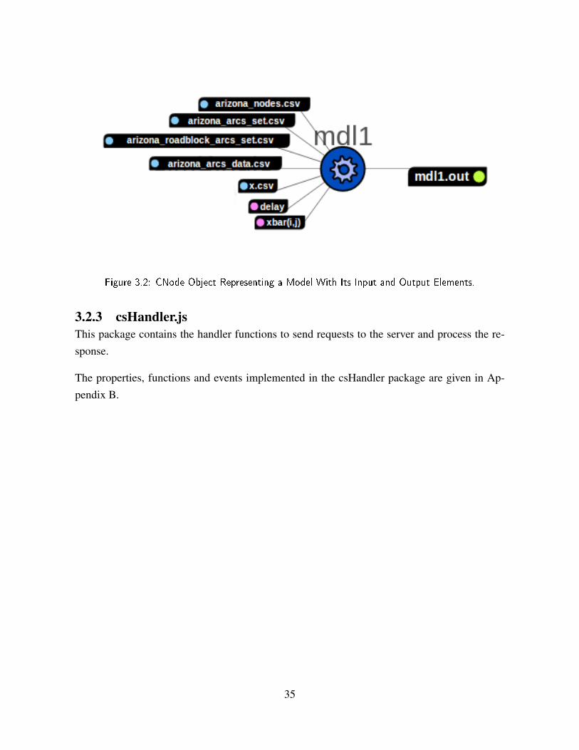
Figure 3.2: CNode Object Representing a Model With Its Input and Output Elements.

3.2.3 csHandler.jsThis package contains the handler functions to send requests to the server and process the re-sponse.

The properties, functions and events implemented in the csHandler package are given in Ap-pendix B.

35


36

CHAPTER 4:

The Analysis of Critical Infrastructure

The initial step in modeling infrastructure operation encompasses transforming a massive (net-work) problem into a mathematical model.One of the challenges in modeling these infrastruc-tures is that they typically do not exist in isolation of one another as mentioned in Chapter 1.For instance, the operation of natural gas infrastructure is dependent on electricity to pump thenatural gas through the pipe network. Similarly, electricity infrastructure depends on naturalgas to produce electricity. We can say that these two infrastructures are interdependent. So inorder to build operational models of infrastructure systems, we need to understand the nature ofthese interdependencies clearly.

Real-world infrastructures demonstrate certain attributes in their interdependencies. Rinaldi(2004) evaluates these attributes and classifies the interdependencies. Based on this classifi-cation, Dixon (2011) suggests several formulations that are proved to be useful for modelingcritical infrastructures with and without isolation.

According to Rinaldi (2004) there are four classes of interdependencies:

• Physical Interdependency: Interdependency for two infrastructures when the state of eachdepends upon the material output(s) of the other. We can observe the physical interde-pendencies in the form of physical linkages or connections among elements of the infras-tructures.• Cyber Interdependency: An infrastructure has a cyber interdependency if its state de-

pends on the data flow through the information infrastructure. The computerization andautomation of modern infrastructures have led to pervasive cyber interdependencies.• Geographic Interdependency: Geographic interdependency exists if a local environmen-

tal event can create state changes in the collocated elements of two infrastructures.• Logical Interdependency: There exists a logical interdependency if the state of each de-

pends upon the state of the other via some mechanism out of the former interdependen-cies. For instance, various political decisions and legal issues can give rise to a logicallinkage among two or more infrastructures.

It is possible to formulate these interdependencies using various formulations. We can see themodel formulations for various interdependent infrastructure types each of which also includes

37

an attacker and defender problem formulation in Dixon (2011):

• Multiple Independent Operators: In this formulation, the modeler assumes that each in-frastructure is independent and operated by a separate system operator who tries to opti-mize his own infrastructure. The concept of a global manager is introduced to minimizethe cost of operating the entire collection of infrastructures. This is basically achieved byusing a common objective function with different weights assigned to each infrastructureto represent the importance of associated infrastructure.• Direct Cost-Based Dependence: This formulation takes into consideration the impact of

disrupted arcs or nodes in one infrastructure. Generic values are used to represent the costeffect of interdicted nodes and arcs.• Indirect Commodity Flow Dependence: This formulation mainly deals with the physical

dependency mentioned before. This dependency is also divided into five types (input,

shared, exclusive-or, mutual and co-location) which intuitively describes the mathemati-cal relations to be applied to input and output elements that are related to another infras-tructure.

In this research, we have limited our scope to include physical interdependencies making use ofthe indirect commodity flow dependence formulation.

When we examine the formulations and scripts in Dixon (2011), we can estimate the workloadassociated with representing all infrastructures in one script file and numerous input files. Wehave noticed that most of the models in Dixon (2011) can be decomposed in a useful level. Wehave built scripts that take advantage of the decomposable structure in these models.

4.1 Decoupled Infrastructure ModelsThe critical infrastructure models in Dixon (2011) and other research are formulated usingone objective function to solve the problem at once. We call these models monolithic mod-els. Monolithic models suffer from various problems as mentioned before. In order to dealwith these problems, we decompose infrastructure models to create stand-alone models. Wedecouple these models by implementing their own objective function and incorporating the de-pendency commodities as input and output elements of the model. In this way, each decoupledinfrastructure model (DIM) becomes executable on its own.

After decoupling the models, we have used the following notation which is common to otherinfrastructure models:

38

Indices and Setsr ∈ R infrastructures in a super-systemn ∈ N nodes in an infrastructure (alias i, j,k, l)(i, j) ∈ A⊆ N×N directed arcsData [units]brn ‘internal’ supply of commodity at node n of infrastructure r [units]sPenrn penalty for ‘internal’ commodity shortage at node n of infrastructure r [cost/unit]uri j capacity of arc (i, j) ∈ A of infrastructure r [commodity/unit]cri j cost per-unit of operating arc (i, j) ∈ A of infrastructure r [cost/unit]Vrn ‘external’ demand of commodity at node n of infrastructure r [commodity units]vPenrn penalty for ‘external’ commodity shortage at node n of infrastructure r [cost/unit]qri j additional cost per-unit of operating interdicted arc (i, j) ∈ A of infrastructure r

[cost/unit]Wri j =1 if arc (i, j) ∈ A is available, = 0 otherwise on infrastructure r [binary]Decision Variables[units]Yri j flow of commodity on arc (i, j) ∈ A of infrastructure r [commodity units]SHORTrn ‘internal’ shortage of commodity at node n of infrastructure r [commodity units]V SHORTrn ‘external’ shortage of commodity at node n of infrastructure r [commodity units]

In what follows, specifically we have infrastructure 1 and infrastructure 2.The Formulation of DIM1The operator’s model for infrastructure 1 is as follows:

minY,SHORT,V SHORT

∑(i, j)∈A

(c1i j + q1i j )Y1i j + ∑n∈N

(sPen1nSHORT1n + vPen1n V SHORT1n) (4.1)

s.t. ∑j:(i, j)∈A

Y1n j− ∑i:(i,n)∈A

Y1in−SHORT1n−V SHORT1n = b1n− V1n ∀n ∈ N (4.2)

0≤ Y1i j ≤ u1i j W1i j ∀(i, j) ∈ A (4.3)

SHORT1n ≥ 0,V SHORT1n ≥ 0 ∀n ∈ N (4.4)

39

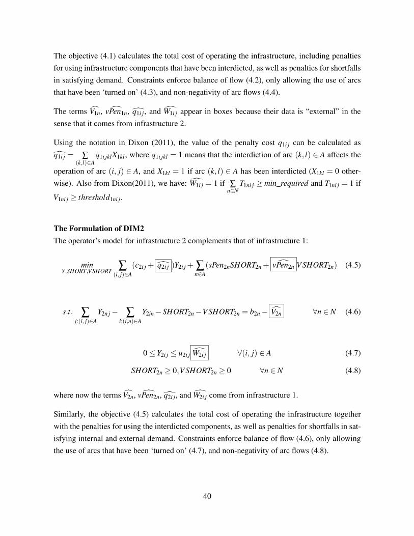
The objective (4.1) calculates the total cost of operating the infrastructure, including penaltiesfor using infrastructure components that have been interdicted, as well as penalties for shortfallsin satisfying demand. Constraints enforce balance of flow (4.2), only allowing the use of arcsthat have been ‘turned on’ (4.3), and non-negativity of arc flows (4.4).

The terms V1n, vPen1n, q1i j, and W1i j appear in boxes because their data is “external” in thesense that it comes from infrastructure 2.

Using the notation in Dixon (2011), the value of the penalty cost q1i j can be calculated asq1i j = ∑

(k,l)∈Aq1i jklX1kl , where q1i jkl = 1 means that the interdiction of arc (k, l) ∈ A affects the

operation of arc (i, j) ∈ A, and X1kl = 1 if arc (k, l) ∈ A has been interdicted (X1kl = 0 other-wise). Also from Dixon(2011), we have: W1i j = 1 if ∑

n∈NT1ni j ≥ min_required and T1ni j = 1 if

V1ni j ≥ threshold1ni j.

The Formulation of DIM2The operator’s model for infrastructure 2 complements that of infrastructure 1:

minY,SHORT,V SHORT

∑(i, j)∈A

(c2i j + q2i j )Y2i j + ∑n∈A

(sPen2nSHORT2n + vPen2n V SHORT2n) (4.5)

s.t. ∑j:(i, j)∈A

Y2n j− ∑i:(i,n)∈A

Y2in−SHORT2n−V SHORT2n = b2n− V2n ∀n ∈ N (4.6)

0≤ Y2i j ≤ u2i j W2i j ∀(i, j) ∈ A (4.7)

SHORT2n ≥ 0,V SHORT2n ≥ 0 ∀n ∈ N (4.8)

where now the terms V2n, vPen2n, q2i j, and W2i j come from infrastructure 1.

Similarly, the objective (4.5) calculates the total cost of operating the infrastructure togetherwith the penalties for using the interdicted components, as well as penalties for shortfalls in sat-isfying internal and external demand. Constraints enforce balance of flow (4.6), only allowingthe use of arcs that have been ‘turned on’ (4.7), and non-negativity of arc flows (4.8).

40

4.2 The Optimization of DIMs Using The TALOS Computa-tion Server

We have analyzed an example where infrastructure 1 depends on infrastructure 2, which doesnot depend on anything. These infrastructures are shown in Figure 4.1. Each infrastructureconsists of three nodes which are partitioned into p and pp internal nodes. Node splitting isa common practice in network flow optimization. It allows us to put a capacity on a node,expose a dependency at a node on another infrastructure, and expose a node as vulnerable in aninterdiction model, where we typically target arcs for interdiction.

Figure 4.1: Decoupled Infrastructure Model 1 and 2.

Solving for the combined solution works as follows:

1. Determine appropriate penalties on unmet requirements1.1. Update W1i j = 1 (all arcs available)1.2. Solve DIM11.3. Record result as best value1.4. Solve DIM1 in a loop

• Update W1i j (a unique combination of dependent arcs’ state for each cycle)• Solve for optimal solution• Calculate difference from best and record as penalty

2. Run super-system in a loop2.1. Solve DIM2

• Initialize q2i j = 0 (no arcs are interdicted)

41

• Initialize W2i j = 1 (all arcs are available)• Update V2n to satisfy all dependent arcs of DIM1• Increment vPen2n

• Solve for optimal solution• Notify DIM1 about the supported external arcs

2.2. Solve DIM1• Initialize q1i j = 0 (no arcs are interdicted)• Update W1i j using the notification sent by DIM2• Initialize V1n = 0 (no external demand)• Increment vPen1n = 0 (no external demand)• Solve for optimal solution• Notify DIM2 about the redundant support

2.3. Solve DIM2• Initialize q2i j = 0 (no arcs are interdicted)• Initialize W2i j = 1 (all arcs are available)• Update V2n to satisfy only needed arcs of DIM1• Solve for optimal solution• Calculate and record total penalty paid• Record DIM1 and DIM2 objective values

The model scripts implemented in GAMS language and associated data files are uploaded tothe TALOS Computation Server. The TALOS Computation Server generates the followingrepresentation for each model.

Figure 4.2: Decoupled Infrastructure Model 1. Figure 4.3: Decoupled Infrastructure Model 2.

The elements on the left of each model represent the input elements and the ones on the rightrepresent expected output files.

42

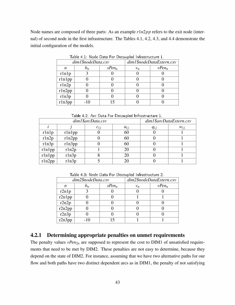
Node names are composed of three parts: As an example r1n2pp refers to the exit node (inter-nal) of second node in the first infrastructure. The Tables 4.1, 4.2, 4.3, and 4.4 demonstrate theinitial configuration of the models.

Table 4.1: Node Data For Decoupled Infrastructure 1.

dim1$nodeData.csv dim1$nodeDataExtern.csvn bn sPenn vn vPenn

r1n1p 3 0 0 0r1n1pp 0 0 0 0r1n2p 0 0 0 0

r1n2pp 0 0 0 0r1n3p 0 0 0 0

r1n3pp -10 15 0 0

Table 4.2: Arc Data For Decoupled Infrastructure 1.

dim1$arcData.csv dim1$arcDataExtern.csvi j ci j ui j qi j wi j

r1n1p r1n1pp 0 60 0 1r1n2p r1n2pp 0 60 0 1r1n3p r1n3pp 0 60 0 1

r1n1pp r1n2p 1 20 0 1r1n1pp r1n3p 8 20 0 1r1n2pp r1n3p 5 20 0 1

Table 4.3: Node Data For Decoupled Infrastructure 2.

dim2$nodeData.csv dim2$nodeDataExtern.csvn bn sPenn vn vPenn

r2n1p 3 0 0 0r2n1pp 0 0 1 1r2n2p 0 0 0 0

r2n2pp 0 0 0 0r2n3p 0 0 0 0

r2n3pp -10 15 1 1

4.2.1 Determining appropriate penalties on unmet requirementsThe penalty values vPen2n are supposed to represent the cost to DIM1 of unsatisfied require-ments that need to be met by DIM2. These penalties are not easy to determine, because theydepend on the state of DIM2. For instance, assuming that we have two alternative paths for ourflow and both paths have two distinct dependent arcs as in DIM1, the penalty of not satisfying

43

Table 4.4: Arc Data For Decoupled Infrastructure 2.

dim2$arcData.csv dim2$arcDataExtern.csvi j ci j ui j qi j wi j

r2n1p r2n1pp 0 60 0 1r2n2p r2n2pp 0 60 0 1r2n3p r2n3pp 0 60 0 1

r2n1pp r2n2p 5 20 0 1r2n1pp r2n3p 8 20 0 1r2n2pp r2n3p 5 20 0 1

both of the dependent arcs is not simply the total of penalty values for not satisfying each de-pendent arc. Total penalty should be much higher than the summation of each penalty value,because the flow in DIM1 is totally blocked.

If we enumerate a range of possible penalty values, it is possible to calculate the total penaltyvalues for all possible states of dependent arcs. At this point, the TALOS Computation Server isuseful for generating total penalty values exhaustively. The number of model runs required forgenerating these values is 2d where d is the number of dependent arcs and nodes. This numberwill grow very quickly for the models with a higher number of dependent arcs.

In order to generate the total penalty values DIM1 needs, we have written the following script.The global variable best represents the optimal cost of operating the system with all dependentarcs satisfied. And the global variable vPenTotal is used for storing the total penalty values.Variables that are used to keep track of optimalcost and total penalty are initialized with var

keyword.

A single run is performed for DIM1 with pretasks to turn on the dependent arcs and a posttaskto assign the Z value to the global variable best.

1 var vPenTotal = 0

2 var best = 0

3 var i = 0, j = 0

4 step #start->dim1

5 pretask dim1$arcDataExtern.csv[4,3]<-override(1)

6 pretask dim1$arcDataExtern.csv[5,3]<-override(1)

7 posttask best<-dim1$Z

8 end step

44

We have implemented the loop structure to be used with ‘loop while(condition)’ and ‘end loop’keywords. Nested loops are used to change the values of global variables i and j and run DIM1four times. The script needed for defining the loops and global task is given below.

9 loop while(i<2)

10 task j<-0

11 loop while(j<2)

12 step #start->dim1

13 pretask dim1$arcDataExtern.csv[4,3]<-override(i)

14 pretask dim1$arcDataExtern.csv[5,3]<-override(j)

15 posttask vPenTotal<-dim1$Z-best

16 posttask inc(j)

17 end step

18 end loop

19 task inc(i)

20 end loop

Having defined the nested loop structures, a step to run DIM1 is defined with pretasks to updatethe state of dependent arcs with i and j values and a posttask to assign vPenTotal the differencebetween the Z value of DIM1 and the value of best. The global variables i and j are reset andincremented with global tasks. After initializing the global variables we define the steps in theform of ‘step from->to’ in which to represents the actual model to be run (from is provided tokeep track of the sequences). Pretasks and posttasks are defined using the pretask and posttask

keywords.

At this point, we can type the command write to record the super-system design we have created.This will give us an opportunity to run the performJSON command which runs the saved super-system design. Finally we use the run command to execute the super-system design.

21 run

Running the script generates the repeated sequences of the following segment:

running with param:

---------------------------------

*** Running step #start->dim1 ***

45

** performing preTasks **

overriding values in dim1$arcDataExtern.csv

overriding values in dim1$arcDataExtern.csv

**** Normal completion ****

objective: 123.000000

mipSol: None

finalSol: None

** performing postTasks **

best<-123.0

---------------------------------

In each segment, we can observe the intermediate objective value of the step and changingglobal variables under the tasks title.

When a model is run and a global variable is changed multiple times, no information is lost.Past values of each variable are stored by the TALOS Computation Server. Using the tracecommand, we can get all values assigned to the global variables including the Z value of DIM1.

22 trace

------------------------------------------------------------

**** Trace Record ****

i$trace: [0.0, 1.0, 2.0]

best$trace: [0.0, 123.0]

vPenTotal$trace: [0.0, 27.0, 6.0, 0.0, 0.0]

j$trace: [0.0, 0.0, 1.0, 2.0, 0.0, 1.0, 2.0]

dim1$Z: [123.0, 150.0, 129.0, 123.0, 123.0]

------------------------------------------------------------

The trace record reveals that failing to satisfy the dependent arcs (r1n1pp,r1n2p) and (r1n1pp,

r1n3p) incurs 27 units of penalty. Similarly, we can see that failing to satisfy only the dependentarc (r1n1pp,r1n2p) requires 6 units of total penalty. However, satisfying all dependent arcs orfailing to satisfy the dependent arc (r1n1pp,r1n3p) requires no penalty. Total penalty valuesare shown in Figure 4.4.

Failing to satisfy both dependent arcs yields a totally blocked flow as shown in Figure 4.5 andfailing to satisfy either one of the dependent arcs yields the network flows given in Figure 4.6

46

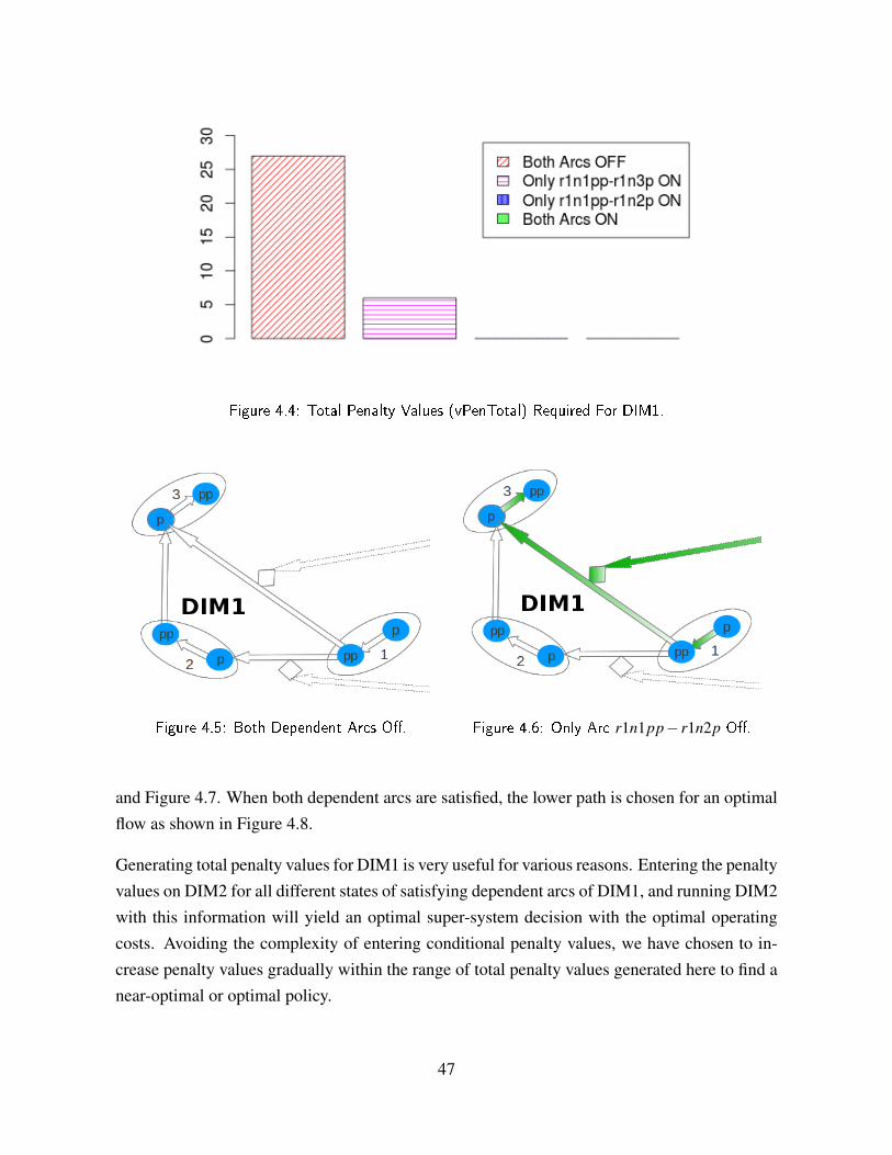
Figure 4.4: Total Penalty Values (vPenTotal) Required For DIM1.

Figure 4.5: Both Dependent Arcs O�. Figure 4.6: Only Arc r1n1pp− r1n2p O�.

and Figure 4.7. When both dependent arcs are satisfied, the lower path is chosen for an optimalflow as shown in Figure 4.8.

Generating total penalty values for DIM1 is very useful for various reasons. Entering the penaltyvalues on DIM2 for all different states of satisfying dependent arcs of DIM1, and running DIM2with this information will yield an optimal super-system decision with the optimal operatingcosts. Avoiding the complexity of entering conditional penalty values, we have chosen to in-crease penalty values gradually within the range of total penalty values generated here to find anear-optimal or optimal policy.

47

Figure 4.7: Only Arc r1n1pp− r1n3p O�. Figure 4.8: Both Dependent Arcs On.

4.2.2 Designing and running the super-system with different vPenn valuesFor this example, considering the different total penalty values ranging from 0 to 27, and run-ning the super-system with vPenn values assigned to DIM2 ranging from 1 to 14, we can achievea near-optimal or optimal policy to minimize operating costs of overall system. Using an upperlimit of 14 will make sure that failing to satisfy both dependent arcs on DIM1 is punished with28 units of total penalty which includes the maximum total penalty we have generated before.However, DIM2 is overcharged with 14 units of total penalty when it fails to satisfy the depen-dent arc (r1n1pp,r1n3p) while the actual total penalty generated during the previous stage iszero.

Total penalty has different meanings for operators of DIM1 and DIM2, and the manager ofsuper-system. The operator of DIM1 will consider the total penalty as a way of motivating theoperator of DIM2 to satisfy his dependent arcs. The operator of DIM1 is the one to decide thevalue of total penalty. This value should not be higher than what is needed to maintain overallsystem optimality. According to the operator of DIM2, total penalty is a value he needs to payto the operator of DIM1 in case he fails to satisfy any external dependency. For the manager ofthe super-system, total penalty is an artificial cost that does not effect the operating cost of thesuper-system in the sense that it is transferred from one infrastructure to another; thus, it staysinside the super-system.

The initial configuration of DIM1 necessarily reflects these assumptions; q1i j = 0 (no arcs areinterdicted), W1i j = 1 (all arcs are available), V1n = 0 (no external demand), vPen1n = 0 (noshortfall penalty for external demand).

48

After running DIM1 with these parameters we can generate the file ext1.csv which includes thearcs that are needed for an optimal minimum-cost flow. Next, we need to update the value ofthe parameter v2n in nodeDataExtern.csv shown in Table 4.3 which belongs to DIM2. Initialpenalty value vPen2n for not satisfying external demand at r2n1pp is 1. Now we are ready to runDIM2 with updated values. Running DIM2 will generate ext2.csv which includes the binaryvalue Provided which yields 1 when node r2n1pp satisfies the external demand. This valueneeds to be written on the value of w1i j of arc (r1n1pp,r1n2p) located in arcDataExtern.csvshown in Table 4.2. Objective function value of DIM2 must be recorded. After running DIM2we will be able observe if the operator of DIM2 is convinced to satisfy the external demand.

Finally we need to run DIM1 with the updated configuration to see the improvement afterthe DIM2’s decision to satisfy the external demand or not. As we can perceive, the value ofvPen2n is the immediate motivation for the operator of DIM2. The amount of this penaltyand the decision of DIM2’s operator will determine the value of vPenPaid located in ext2.csv.vPenPaid is an artificial penalty used to influence the behaviour of one operator analogous tothe total penalty. We may consider the value of vPenPaid as the amount taken from the operatorof DIM2 and given to DIM1. The equation for vPenPaid is given in 4.9.

vPenPaid = ∑n∈N

( vPen2nV SHORT2n) (4.9)

And we can define netCost as follows:

netCost = ZDIM1 +ZDIM2− vPenPaidDIM2. (4.10)

Using either the scripting language on the command-line interface or the web-GUI of the TA-LOS Computation Server it is possible to define and perform these tasks. As we have mentionedbefore the value vPen2n, determined by the operator of DIM1, will have a significant impact onthe super-system optimization. In order to run the sequence of DIM1, DIM2 and DIM1 againwith different values of vPen2n we use the loop structure implemented in the scripting language.

1 var vPenn = 0

2 var vPennPaid = 0

3 var totalCost = 0

4 var netCost = 0

5 loop while(vPenn<15)

49

The first step in the loop is step #start->dim2. In this step, vPenn is incremented and writteninto DIM2’s vPen2n values in nodeDataExtern.csv file of DIM2, and v2n values of DIM2 areinitialized with value 1 as pretasks. After running DIM2 with these pretasks, binary valuesProvided in ext2.csv file of DIM2 is written into w2i j values of DIM1 as posttasks.

6 step #start->dim2

7 pretask inc(vPenn)

8 pretask dim2$nodeDataExtern.csv[2,1]<-override(1)

9 pretask dim2$nodeDataExtern.csv[6,1]<-override(1)

10 pretask dim2$nodeDataExtern.csv[2,2]<-override(vPenn)

11 pretask dim2$nodeDataExtern.csv[6,2]<-override(vPenn)

12 posttask dim1$arcDataExtern.csv[4,3]<-override(dim2$ext2.csv[2,1])

13 posttask dim1$arcDataExtern.csv[5,3]<-override(dim2$ext2.csv[6,1])

14 end step

The next sequence includes the step from DIM2 to DIM1 in which DIM1 is executed. In thisstep DIM1 is solved with the provided support from DIM2. After running DIM1, the TALOSComputation Server performs posttasks to check if DIM1 is not using a dependent arc that hasbeen supported by DIM2. Such a case will yield a redundant cost on DIM2 and the overallsystem.

Formulating an equation to satisfy the conditions shown in Table 4.5 is necessary in order toaddress this problem.

Table 4.5: Condition Table For Finding Redundancy.

Inputs OutputW1i j isNeeded1i j V2n

1 0 01 1 10 0 1

When the availability of a dependent arc (W1i j) is 1 and it is needed for an optimal flow onDIM1, V2n must be assigned 1. When the availability of a dependent arc (W1i j) is 1 and it is notneeded for an optimal flow on DIM1, V2n must be assigned 0. However, when the availabilityof a dependent arc (W1i j) is 0, we do not have any information if that arc is needed or not,and DIM2 keeps paying a penalty for that dependent arc. The formulation constructed to avoidredundant penalty is given in 4.11.

50

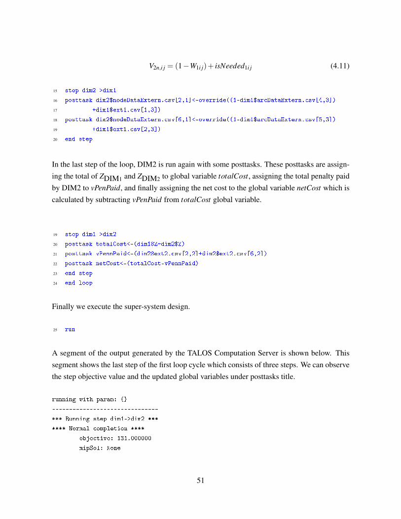
V2n,i j = (1−W1i j)+ isNeeded1i j (4.11)

15 step dim2->dim1

16 posttask dim2$nodeDataExtern.csv[2,1]<-override((1-dim1$arcDataExtern.csv[4,3])

17 +dim1$ext1.csv[1,3])

18 posttask dim2$nodeDataExtern.csv[6,1]<-override((1-dim1$arcDataExtern.csv[5,3])

19 +dim1$ext1.csv[2,3])

20 end step

In the last step of the loop, DIM2 is run again with some posttasks. These posttasks are assign-ing the total of ZDIM1 and ZDIM2 to global variable totalCost, assigning the total penalty paidby DIM2 to vPenPaid, and finally assigning the net cost to the global variable netCost which iscalculated by subtracting vPenPaid from totalCost global variable.

19 step dim1->dim2

20 posttask totalCost<-(dim1$Z+dim2$Z)

21 posttask vPennPaid<-(dim2$ext2.csv[2,2]+dim2$ext2.csv[6,2])

22 posttask netCost<-(totalCost-vPennPaid)

23 end step

24 end loop

Finally we execute the super-system design.

25 run

A segment of the output generated by the TALOS Computation Server is shown below. Thissegment shows the last step of the first loop cycle which consists of three steps. We can observethe step objective value and the updated global variables under posttasks title.

running with param: {}

-------------------------------

*** Running step dim1->dim2 ***

**** Normal completion ****

objective: 131.000000

mipSol: None

51

finalSol: None

** performing postTasks **

totalCost<-281.0

vPennPaid<-2.0

netCost<-279.0

-------------------------------

We display the trace information to obtain the values of global variables.

26 trace

------------------------------------------------------------

**** Trace Record ****

netCost$trace: [0.0, 279.0, 279.0, 279.0, 279.0, 279.0, 279.0, 279.0,

259.0, 259.0, 259.0, 259.0, 259.0, 259.0, 259.0, 259.0]

totalCost$trace: [0.0, 281.0, 283.0, 285.0, 287.0, 289.0, 291.0,

293.0, 267.0, 268.0, 269.0, 270.0, 271.0, 272.0, 273.0, 259.0]

vPennPaid$trace: [0.0, 2.0, 4.0, 6.0, 8.0, 10.0, 12.0, 14.0, 8.0,

9.0, 10.0, 11.0, 12.0, 13.0, 14.0, 0.0]

dim2$Z: [131.0, 131.0, 133.0, 133.0, 135.0, 135.0, 137.0, 137.0, 139.0,

139.0, 141.0, 141.0, 143.0, 143.0, 144.0, 144.0, 145.0, 145.0, 146.0,

146.0, 147.0, 147.0, 148.0, 148.0, 149.0, 149.0, 150.0, 150.0, 151.0,

136.0]

dim1$Z: [150.0, 150.0, 150.0, 150.0, 150.0, 150.0, 150.0, 123.0, 123.0,

123.0, 123.0, 123.0, 123.0, 123.0, 123.0]

vPenn$trace: [0.0, 1.0, 2.0, 3.0, 4.0, 5.0, 6.0, 7.0, 8.0, 9.0, 10.0,

11.0, 12.0, 13.0, 14.0, 15.0]

------------------------------------------------------------

The following plots are generated using the output of command trace.

As we can see in Figure 4.10, the operator of DIM2 is not convinced to satisfy external demanduntil the 7th run. The Z value (objective function value) of DIM2 is gradually increasing untilthe 15th loop (29th DIM2 run). We can observe that DIM2 is run twice in each loop. The secondrun of each loop yields the Z value that is updated using the equation in 4.11. Until the 29th

DIM2 run there is no redundancy in DIM2’s supporting external arcs. However, before the30th DIM2 run, DIM1 detects a redundancy caused by DIM2’s prior decision to support bothdependent arcs during the 29th DIM2 run. The network flow demonstrating this redundancy is

52

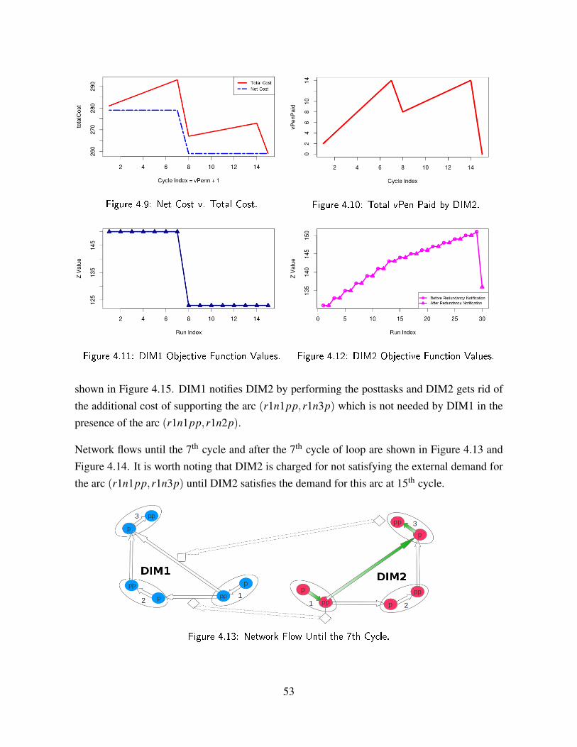
Figure 4.9: Net Cost v. Total Cost. Figure 4.10: Total vPen Paid by DIM2.

Figure 4.11: DIM1 Objective Function Values. Figure 4.12: DIM2 Objective Function Values.

shown in Figure 4.15. DIM1 notifies DIM2 by performing the posttasks and DIM2 gets rid ofthe additional cost of supporting the arc (r1n1pp,r1n3p) which is not needed by DIM1 in thepresence of the arc (r1n1pp,r1n2p).

Network flows until the 7th cycle and after the 7th cycle of loop are shown in Figure 4.13 andFigure 4.14. It is worth noting that DIM2 is charged for not satisfying the external demand forthe arc (r1n1pp,r1n3p) until DIM2 satisfies the demand for this arc at 15th cycle.

Figure 4.13: Network Flow Until the 7th Cycle.

53

Figure 4.14: Network Flow After the 7th Cycle and the 15th Cycle.

Figure 4.15: Intermediate Network Flow Before the Redundancy Noti�cation at the 15th Cycle.

When we have a look at total cost value on Figure 4.9 we can see that it is increasing graduallyuntil the 7th cycle and decreasing dramatically at the 8th cycle. This is because the operator ofDIM2 is convinced to support one of the dependent arcs (r1n1pp,r1n2p) which saves DIM1from blocked state and decreases DIM1 operating cost by 27. After this point, vPen2n is stillbeing increased and DIM2 is charged with the penalty of not satisfying the arc (r1n1pp,r1n3p)

until the 14th cycle. We observe another dramatic decrease in total cost at the 15th cycle whichis caused by DIM1’s notification about the redundant support for the arc (r1n1pp,r1n3p).

As mentioned before, the super-system operator must focus on the net cost which also decreasesafter convincing the operator of DIM2 to satisfy the external demand and is fixed at the samelevel. At the 15th cycle totalcost converges to netcost. At this point DIM2 is not charged witha penalty (vPenPaid = 0).

The result reveals that the optimal super-system decision is to declare a penalty of 14 only forfailing to satisfy the arc (r1n1pp,r1n2p). This policy will keep the arc (r1n1pp,r1n2p) ondespite the increased cost of operating DIM2. This result is generated assuming equal weightsfor the cost values of operating each infrastructure.

54

The methodology for solving a super-system optimization problem consisting of more than twointerdependent infrastructures with a large number of nodes and arcs is not basically differentfrom the technique we have used on the TALOS Computation Server.

The crucial issue about making use of the TALOS Computation Server is implementing themodels with well-formatted input and output files so that the model can be reused.

55


56

CHAPTER 5:

Conclusions and Future Work

We conclude by summarizing our work and suggesting several ideas for future research anddevelopment on the TALOS Computation Server and the analysis of critical infrastructures.

5.1 ConclusionsIn this thesis, we examine the steps followed by researchers while solving an optimizationproblem. We explain the challenges associated with modeling and solving interdependent in-frastructure systems. Evaluating the current practices, we detect the deficiencies in current useof computational tools. As a result of this evaluation, we capture and analyze the requirementsfor a cloud-based computation server. Some of the features expected from a computation serverare model integrity checking, meta-data generation, visualization, reporting, error handling,graphical user interface, scripting on terminal and super-system design to model interdependentinfrastructure systems.

We propose an architecture to address the requirements for a computation server. In accordancewith our principal design decisions, we implement the TALOS Computation Server.

We present decoupled infrastructure models that can be generalized and used for real-worldinfrastructure systems. Decoupled infrastructure systems are stand-alone, executable optimiza-tion models decomposed from monolithic infrastructure systems model. We demonstrate theanalysis of interdependent infrastructures using the TALOS Computation Server. The easeand efficiency of designing, running and debugging the super-system representing the criti-cal infrastructure systems on the TALOS Computation Server for our analysis reveals that therequirements are correctly captured and mapped into the architectural design.

5.2 Future WorkWe have designed the TALOS Computation Server to be used with the GAMS optimization lan-guage considering the needs of operations research students and faculty at Naval PostgraduateSchool. However, improving the user experience and extending the optimization interpreters toinclude other optimization languages will allow analysts, decision makers and researchers fromother departments to make use of the services provided by our computation server.

57

Security related requirements which are crucial for a distributed system are not addressed inthis research. Security means correct behavior in the face of an intelligent adversary. Threeimportant properties in a secure system are confidentiality, integrity, and availability (Salehiet al., 2007). The most important tactic to be used at the architectural level will be improvingthe access control of the TALOS Computation Server. In this way, it will be possible to storevaluable models and data sets.

We have presented decoupled infrastructure models and proposed a two-phased method foroptimizing the cost of operating the overall system. In this way, we have managed to overcomethe problems associated with the monolithic models. Similar decomposition methods mustbe evaluated and tested on the TALOS Computation Server. Every model run on the TALOSComputation Server is tagged with metadata and becomes reusable.

Similarly, most common optimization models can be made available to the registered users byhosting them on the TALOS Computation Server. This will help minimize the duplicated effortsin the optimization community.

Promoting the TALOS Computation Server to a widely used system will require implementingAPIs so that the developers can make use of the services provided by the server in their ownapplications.

Optimization is also commonly used with simulation tools. Incorporating lightweight simula-tion tools such as Sigma (Schruben, 1990) in the TALOS Computation Server will be helpfulfor facilitating the related analyses.

58

APPENDIX A:

Server-Side Implementation Details

A.1 agent PackageThe agent package contains a helper function getMdls which is responsible for fetching themetadata that was automatically generated during the ‘generate model’ process. The content ofeach model’s metadata is used to populate a graphical representation of each model in the webGUI (client side).

A.2 fileCtrl PackagegetInputFiles: This function extracts input files by parsing through the GAMS script. Parsingis performed by making use of the ‘$INCLUDE’ statements in the GAMS script. Python’sStandard Regular Expression library provides conveniences to detect the occurrence of thesestatements and filter out the files included as input files. The input file list will be useful whilechecking the model integrity, generating metadata and finally binding model elements withthose of another.

Parameters

fName:File nameReturn values

inputFList: Input file list

getParams: This function extracts Parameters by parsing through the gams script. Parsingis performed by making use of the ‘PARAMETER(S)’ statements in the GAMS script. Bothlowercase and uppercase statements are detected to extract Parameters. In GAMS parametersmay be a single-value (scalar) or multi-dimensional. Both types are detected by this function.

Parameters

fName:File nameReturn values

params: Parameter list

59

checkFiles: This function checks if all files specified in the file list exist. This function isimplemented to find missing files by comparing existing input files in the model directory andthe file list given as a parameter. Empty list returned by this function is the desired result interms of file integrity.

Parameters

fList: File listReturn values

missing: Missing file list

getOutFiles: Extracts output files by parsing through the GAMS script. Parsing is performedby making use of the statement ‘FILE’ both in upper and lowercase. Similarly returned outputfile list will be useful while generating metadata and binding model elements with those ofanother.

Parameters

fName: File nameReturn values

outputFList: Output file list

getAllFiles: Extracts all files by parsing through the GAMS script. This function calls getOut-Files and getInFiles to populate all files list.Parameters


allF: All files list

displayOutput: This function displays the content of the file specified as argument.

Parameters


None.

60

A.3 mdlPack Package

A.3.1 MdlPack ClassMdlPack class contains the following member functions:

Constructor: Extracts the model script file name using the provided arguments . If no filenameis provided detects the GAMS file in the given directory using detectGms function.ParametersfAddress: GAMS script file addresstargetDir: Target directory (working directory by default)

writeJSON: This function writes the metadata in JSON format. Metadata of a model containsmodel name, input files, output files, author name and date created. These data are written asmetaData.json file in model directory (which has the identical name as the model script fileexcluding the extension). Input/Output files are extracted using the functionalities providedfileCtrl Package.ParametersNoneReturn valuesNone

getPackName: Generates a package file name with .tar extension using the model script filename.ParametersNoneReturn valuesPackage: Package name with .tar extension

createTar: Creates ‘.tar’ file from the files in a given directory. The ‘.tar’ file stands for archivefile which is useful for restoring a model from its initial state and providing the user with areusable model with its metadata if the user prefers downloading the ‘.tar’ package.ParametersNone

61

Return valuesNone

cleanDir: Deletes all files in a temporary upload directory. This functionality is used after thepacking (createTar) is completed.ParametersNoneReturn valuesNone

detectGms: Detects a GAMS file by searching for .gms or .gm extension and certain patternsin this file. In case no file is specified in Constructor, initially this function searches for thefiles with ‘gm’ and ‘gms’ extension. If there are more than one file with these extensions thenthe main model script file is determined using the $TITLE and SOLVE statements which areexpected to be found in the main script file.

ParametersNoneReturn valuesfName Main model script file name

A.4 mdlUnpack Packageextract: This function extracts the files of a compressed archive into working directory.Parameters

NoneReturn values

None

A.5 mediator PackageA.5.1 Mediator ClassConstructor: When Mediator class is initialized global dictionaries and lists are created for allmodels the user has unloaded previously. These dictionaries and lists are:

62

Model Dictionary: This dictionary is populated with mappings from model name to modelobject generated using Factory Class. Global Variables Dictionary: The TALOS ComputationServer captures the objective function value of each model by default. This value is representedas ‘modelName$Z’ where first part before dollar sign represents the model name. By default‘modelName$Z’ maps to an empty list. This list is appended with new objective function valueafter each run of a model.

The user may define a new global variable during super-system design to facilitate interactionsbetween models.

Model Parameters Dictionary: This dictionary is populated with single-valued (scalar) pa-rameters and multi-dimensional parameters. Parameter names in the form of ‘modelName$paramA’are mapped into user-defined values in order to run the model with a specific parameter.

Function Dictionary: The TALOS Computation Server provides some functions to facilitatebindings between models. These functions are inc, dec and override. These keywords aremapped into the object address f of their associated functions. While override function is usedfor almost every pretask or posttask, the other functions are expected be more useful whilerunning some models in a loop.

Input List: This list is populated with the input file names using the fileCtrl Package. If theuser prefers to use command-line interface this list is used to verify that the files associated inpretask or posttask are valid.

Output List: This list is populated with the output file names using the fileCtrl Package. Simi-larly this list is used for verification of binding while defining pretask or posttask on command-line interface.

The following member functions give the Mediator Class desired functionalities:

override: Overrides a target file using the source file/file items. Parameters

target: Target file or file item (selected rows and columns only for .csv files)source: Source file or file tem (selected rows and columns only for .csv files)Return values

None

63

inc: Increments the given valueParameters

x: Numerical valueReturn values

x+1

dec: Decrements the given valueParameters

x: Numerical valueReturn values

x-1

getValByRef: Extracts the values from .csv value using getValues function after parsing thereference.Parameters

ref: Reference pointing the row col rangeReturn values

modelName: Model NamefileName: input/output file namerowRange: translated row rangecolRange:translated column rangematrix: values from .csv file

getValues: Extracts the specified values from .csv file.Parameters

rowCol: Statement showing the columns and rows intersectionfName: File namefDir: Directory nameReturn values

rowRange: translated row rangecolRange:translated column rangematrix: values from .csv file

64

stripList: Strips off the whitespaces for a given list.Parameters

lst: List to be processedReturn values

tmp: Stripped list

numeric: Evaluates if the given value is numerical.Parameters

s: String valueReturn values

Boolean True means numerical

A.5.2 Model ClassConstructor: After initialization model name, model directory information are assigned toclass variables, and finally the parameters list is populated with parameters. These data arethe only information needed to run a model given that the input files are ready or modifiednecessarily.

getSetFile: Extracts set filename from the GAMS Script using the set name. This functionsearches the SET statement in order to extract set file name.Parameters

setName: Set namefName: GAMS file nameReturn values

setFile: Associated set file (csv)

modifyParams (Experimental): Modifies the main GAMS script to make parameters usefulfor Mediator while using the complete parameter list. Modification consists of transforming theparameter into a control variable in GAMS script.Parameters

pList: Parameter list include single and vector parameters

65

Return values:

None

getParams: Extracts parameters from the GAMS file using PARAMETER(S) statement bothuppercase and lowercase.Parameters

NoneReturn values

params : Parameter list containing single and vector parameters

run: Runs the model with the given key-worded arguments. Key worded arguments consist ofparameter and numerical value pairs. Running with parameters is only available if parametersare successfully transformed using modifyParams and the given parameter is a single-valuedparameter included in the parameter list of Mediator Class.Parameters

**kwargs: Key-worded arguments Return values

msg: Message Normal or Errorobjective: Objective valuemipSol : MIP solution valuefinalSol: Final solution value

A.5.3 Connector ClassTask struct contains func, var and value properties. This struct may be considered as a statementconsisting of an assignment statement. That is, ‘var’ is assigned the returning value of ‘func’with ‘value’ as its argument. In Python using a named tuple is efficient way to implement astruct.

Constructor: When Connector Class is initialized pretask and posttask lists are initialized.Connector should be given the previous model name as ‘from’ and present model name as‘to’. The other information needed to generate the connector and run through this connectoris provided by Mediator instance. The first step that requires running the first model will havea virtual previous model called ‘#start’. The ‘#’ sign at the beginning of this model name is

66

used to ensure that this model name will not be looked up at Model Dictionary populated inMediator.Parameters

frm: Previous modelto: Present modelmediator: Mediator instance to get necessary values and functions

addPre: This function adds a pretask to the pretask list.Parameters

task: Task struct containing task informationReturn values

None

addPost: This function adds a posttask to the posttask list.Parameters

task: Task struct containing task informationReturn values

None

perform: This function performs the pretasks in pretask list, runs the model (given as to) andfinally performs the posttasks in posttask list. After running the model, the objective functionvalue is appended to the Z value list of the model located in Global Variable Dictionary of Me-diator.Parameters

**kwargs: Key-worded Arguments for model runReturn values

None

performTask: This function performs single task either pretask or posttask. This functionalityis needed in the function perform while performing the tasks.Parameters

task: Task struct containing task information

67

Return values

None

createTask: Generates a Task struct with given task information.Parameters

var: Variable/Area to be modifiedvalue: New value or label for valuesfunc: Modification functionReturn values

Task: struct

A.5.4 Loop ClassConstructor: Initializes a connector list called conList, assigns a terminate condition to theterminate variable.Parameters

termCondition: Termination Condition StatementevalFunc: Evaluation function to evaluate termCondition

addCon: Adds a connector to the connector list.Parameters

con: ConnectorReturn values

None

perform: This function keeps performing the steps defined in connectors until the terminationcondition is met.Parameters

NoneReturn values

None

68

A.5.5 Factory ClasscreateModel: Creates Model instanceParameters

name: Model namemDir: Model directoryReturn values

Model: Instance

createConnector: Creates Connector instance.Parameters

frm: Previous modelto: Present modelmediator: Mediator instance to get necessary values and functionsReturn values

Connector: Instance

createLoop: Creates Loop instance.Parameters

termCondition :Termination StatementReturn values

Loop: Instance

A.5.6 Attachment ClassConstructor: Initializes Factory, Mediator instances and attachment dictionary and jsonDataobject.Parameters

None

writeJSON: Writes the populated jsondata into json file called superSystem.json.Parameters

None

69

Return values

None

runJSON: Creates the connectors described in the given attachment data, runs the sequence ofmodels with given pretasks, posttasks, and parameters.Parameters

sModel: Super-system information in JSON formatReturn values

None

performJSON: Creates the connectors described in the default attachment file (superSystem.json)and runs the sequence of models with given pretasks, posttasks and parameters.Parameters

NoneReturn values

None

transform: Transforms provided key-worded arguments into tuple.Parameters

**kwargs: Keyworded argumentsReturn values

Dictionary containing the pairs to be transformed into JSON

cmdLine: Provides the command-line interface to design and run the super-system. Thecommand-line interface accepts the scripting language we developed to facilitate super-systemdesign and running.This scripting language has the following keywords:step mdl1->mdl2: Starts a new step to run mdl2 (mdl1 is used for tracking the trace of multiplemodel run)end step: Finalizes the step designpretask: Defines pretaskposttask: Defines posttask

70

param: Defines parameter if parameter does not exist otherwise assigns value to existing onesrun: Runs the super-system createdquit: Quits the applicationThe functions that can be used within pretask and posttask intructions:override(): Overrides parameter, file or part of a file (.csv format supported)inc(): Increments the given valuedec(): decrements the given value

resolveFunc: Resolves the elements of a task function.Parameters

line: Row containing the pretask/posttask statementReturn values

var: Variablefunc: Function namevalue: New value

getFromTo: Resolves the previous model and present model in step statement.Parameters

line: Row containing the step statementReturn values

frm: From modelto: To Model (From Model used as follow-up information)

resolveParam: Resolves the parameter assignment information in param statement.Parameters

line: Row containing the param statement (multiple parameters separated by comma)Return values

rParam: Dictionary containing parameter names and its value

process: Processes a single line of attachment (either step,end step, pretask, posttask, param orrun)Parameters

71

line: Row containing a valid statement in attachment file or JSON data

72

APPENDIX B:

Client-Side Implementation Details

Client-side implementation consists of three page/packages:

B.1 dashBoard.htmldashBoard.html provides the web interface for the Talos Computation Server. The visual ele-ments displayed on the web interface during the super-system design are shown in Figure B.1.

Figure B.1: The Web Interface For the TALOS Computation Server.

B.2 SGNet.jsSGNet.js consists of two main objects: CNode and Element Objects.

B.2.1 CNode ObjectGraphical representation of a node/model.CNode Object contains the following properties:arcIn: Array of arcs from CNode to each of input elements.arcOut: Array of arcs from CNode to each of input elements.

73

el: Array of all Element ObjectselIn: Array of all Input ElementselOut: Array of all Output Elementgroup: Holder object to aggregate node, node icon and node labelinfo: Node/Model Informationmain: Main Circle object representing the nodename: Node/Model namenumElIn: Total number of input elementsnumElOut: Total number of output elementssetIcon: Icon showing that the node represents a model. When the model is running the icon isanimated with rotation until the model run is completed.stepArc: Dynamic step object that is drawn from the center of one model to another to repre-sent the step (single run sequence). Drawing is performed when the design mode is activated,the node is click and dragged to the desired node. StepArc will be valid only if the mouse isreleased on a valid node/model object. Right clicking on the stepArc will display the elementsready for interaction design. This object has its own mousedown event implemented to facilitatethis visualization.

The following methods are implemented in CNode Object:Constructor: Creates a new CNode Object.Parameters

x: X coordinatey: Y coordinaterad: Radiusmodel: Flag indicating if the node is representing a "model"info: Node information

Element: If the CNode is representing a model, each input or output element of the model isshown as Element Object. Considering the significance and complexity of this object, detailedinformation is provided after CNode Events. down: Down callback function needed for dragevent.Parameters

None

74

getCirIn: Yields the x or y coordinate for each output element by calculating the angle of eachelement to y axis of Cnode.Parameters

eInd: Element IndextElem: Total number of ElementsgiveX: True if X is requested o/w FalseReturn values

x or y coordinate (depending on giveX flag)

getName: Yields the name of the nodeParameters

NoneReturn values

name of the node

hideEl: Hides the elements of the node.Parameters

NoneReturn values

None

highlight: Highlights the outer curve of circleParameters

NoneReturn values

None

highLightOff:Turns off the highlight for the outer curve of circleParameters

None

75

Return values

None

move: Move callback function for drag eventParameters

dx: Change in x axisdy: Change in y axisReturn values

None

showEl: Shows the elements of the nodeParameters

NoneReturn values

None

up: Up callback function for drag eventParameters

NoneReturn values

None

updateConnection: Updates the path of stepArc object and redraws the stepArc objectParameters

dx: Change in x axisdy: Change in y axisReturn values

None

The following events are implemented for CNode Object:drag: Drag event for Cnode.

76

Parameters

move: Move callback function up: Up callback function down: Down callback function

mousedown: Mousedown event for CNodeParameters

None

mouseover: Mousedown event for CNodeParameters

None

mouseup: Mousedown event for CNodeParameters

None

B.2.2 Element Object:If the CNode is representing a model, each input or output element of the model is shown asElement Object. Input elements are positioned on the left side of the model representation(CNode). Blue colored input elements represent the input files (.csv, .gms, .gm, etc.), magentacolored input elements represent the parameters included in the model script while the outputfiles are displayed in green on the right side of the model representation.

Element object contains the following properties:bindNode: Connection point of an element. This object also shows the type of element withdifferent colors. This object contains the folowing property, methods and events to facilitate theinteraction between the elements of different Models.Properties:overrideArc:Arc representing the override process (from source to destination)Methods:down: Callback function for drag functionhighlight: Highlights the bindNode.highlightOff: Turns off the highlight for the bindNode.move: Callback function with parameters dx (Change in x axis), dy (Change in y axis) for drag

77

eventup: Callback function for drag functionupdateConnection: Updates and redraws the connector between the bindNode to another torepresent overriding. This method has the parameters dx (Change in x axis), dy (Change in yaxis).Events:drag: Drag event for bindNode.Parameters

move: Move callback functionup: Up callback functiondown: Down callback functionmousedown: Mousedown event for bindNodeParameters

Nonemouseover: Mousedown event for bindNodeParameters

None

mouseup: Mousedown event for CNodeParameters

None

eText: Element’s label object which contains either the name of the file or parameter imple-mented in model script. This object has the following events implemented:mouseout: Mouseout event for CNodeParameters

Nonemouseover: Mouseover event for CNodeParameters

None

group: Container object holding the Element, its eText(label) and bindNode.

78

Element object has the following constructor:Constructor:Initializes the Element instance with given parameters.Parameters

x : X coordinatey : Y coordinatetxt : LabelfontSize : Font sizeref : Referencecol : ColormName : Model Name

The following events are implemented for Element Object:mouseout: Mouse out event for the ElementParameters

None

mouseover: Mouse over event for the ElementParameters

None

B.3 csHandler.jsProperties implemented in csHandler package:

hH: Height of super-system design div.hW: Width of super-system design div.modelArcs: List holding arcs information (step information)modelNodes: List holding models informationmyGraph: Temporary network (SGNet) onject to visualize results.ph: Super-system Network(SGNet) object

79

query: Process type sent to the TALOS Computation Serverstatus: Name of the status divtotalModel: Number of total models displayed

Methods implemented in csHandler package:

checkServer: Sends ’checkserver’ request to Agent on the TALOS Computation ServerParameters

NoneReturn values

None

errResponse: Displays error message (AJAX error) on status divParameters

NoneReturn values

None

generateMdl: Sends ’generateMdl’ request to Agent on the TALOS Computation ServerParameters

NoneReturn values

None

getResults: Temporary function to display the resultsParameters

NoneReturn values

None

isEmpty: Evaluates if the given dictionary object is empty or notParameters

Dictionary ObjectReturn values

Boolean: True means empty

80

processResponse: Processes the response sent by Agent on the TALOS Computation Server,displays updates and messages on status divParameters

data: Data containing request and user info etc.Return values

Boolean: None

runSuperMdl: Sends ’runSuper’ request with populated stepList to Agent on the TALOS Com-putation ServerParameters

NoneReturn values

None

setSuperSystem: Sets super-system network object calculating given holder div dimensionsand assigns status div name to status variable.Parameters

holderDiv : Name of the div holding super-system networkstatusDiv : Name of the div holding status informationReturn values

None

81


82

REFERENCES

Alderson, D., Brown, G., DiRenzo III, J., Engel, R., Jackson, J., Maule, B., andOnuska, J. (2012). Improving the resilience of coal transport in the port of pitts-burgh - an example of defender-attacker-defender optimization-based decision support.Technical report, Naval Postgraduate School, Monterey, Calfornia. Retrieved fromhttp://calhoun.nps.edu/public/handle/10945/25353.

Amirat, A. and Oussalah, M. (2009). Systematic construction of software architecture supportedby enhanced first-class connectors. Informatica (Slovenia), 33(4):499–509.

Babick, J. P. (2009). Tri-level optimization of critical infrastructure resilience.Master’s thesis, Naval Postgraduate School, Monterey,Ca. Retrieved fromhttp://calhoun.nps.edu/public/handle/10945/4652.

Berzins, V. and Luqi, L. (1991). Software engineering with abstractions. Boston, MA: Addison-Wesley Longman Publishing Co.

Brown, G., Carlyle, W. M., Abdul-Ghaffar, A., and Kline, J. (2011). A defender-attacker opti-mization of port radar surveillance. Naval Research Logistics (NRL), 58(3):223–235.

Brown, G., Carlyle, W. M., Salmeron, J., and Wood, K. (2006). Defending critical infrastruc-ture. Interfaces, 36(6):530–544.

Brown, G. G., Carlyle, W. M., Harney, R. C., Skroch, E. M., and Wood, R. K. (2009). Interdict-ing a nuclear-weapons project. Operations Research, 57(4):866–877.

Brown, G. G., Carlyle, W. M., Salmeron, J., and Wood, K. (2005). Analyzing the vulnerabilityof critical infrastructure to attack and planning defenses. In Tutorials in Operations Research.INFORMS, pages 102–123. Hanover, MD: INFORMS.

Brown, G. G. and Dell, R. F. (2006). Formulating integer linear programs: A rogues’ gallery.Technical report, DTIC Document.

Brown, G. G., Dell, R. F., and Farmer, R. A. (1996). Scheduling coast guard district cutters.Interfaces, 26(2):59–72.

Brown, G. G., Dell, R. F., and Newman, A. M. (2004). Optimizing military capital planning.Interfaces, 34(6):415–425.

83

Brown, G. G., Kline, J. E., Rosenthal, R. E., and Washburn, A. R. (2007). Steaming on convexhulls. Interfaces, 37(4):342–352.

Dell, R. F. (1998). Optimizing army base realignment and closure. Interfaces, 28(6):1–18.

Dell, R. F., Ewing, P. L., and Tarantino, W. J. (2008). Optimally stationing army forces. Inter-faces, 38(6):421–435.

Department of Homeland Security (2010). Risk steering committee, DHS Risk Lexicon. Re-trieved from http://www.dhs.gov/dhs-risk-lexicon. Accessed on 2013-05-02.

Dixon, C. A. (2011). Assessing the vulnerabilities in interdependent infrastructures usingattacker-defender models. Master’s thesis, Naval Postgraduate School, Monterey,Ca. Re-trieved from http://calhoun.nps.edu/public/handle/10945/5606.

Dolan, E. D., Fourer, R., Goux, J.-P., Munson, T. S., and Sarich, J. (2008). Kestrel: An interfacefrom optimization modeling systems to the NEOS server. INFORMS Journal on Computing,20(4):525–538.

Feng, T., Bi, J., Hu, H., and Cao, H. (2011). Networking as a service: a cloud-based networkarchitecture. Journal of Networks, 6(7):1084–1090.

Kruchten, P. (1995). Architectural blueprints — the “4+1” view model of software architecture.IEEE Software, 12(6):42–50.

Martins, G. H. and Dell, R. F. (2008). Solving the pallet loading problem. European Journal ofOperational Research, 184(2):429–440.

Mcheick, H., Qi, Y., and Mili, H. (2011). Scenario-based software architecture for design-ing connectors framework in distributed system. International Journal of Computer ScienceIssues (IJCSI), 8(1):32–41.

Newman, A., Rosenthal, R., Salmeron, J., Brown, G., Price, W., Rowe, A., Fennemore, C., andTaft, R. (2011). Optimizing assignment of tomahawk cruise missile missions to firing units.Naval Research Logistics, 58(3):281–295. 58.

Pahl, C. and Yaoling Zhu1, y. (2009). Model-driven connector development for service-basedinformation system architectures. Journal of Software (1796217X), 4(3):199–209.

84

Rardin, R. L. (1998). Optimization in operations research, volume 166. Upper SaddleRiver:Prentice Hall.

Rinaldi, S. (2004). Modeling and simulating critical infrastructures and their interdependencies.In Proceedings of the 37th Annual Hawaii International Conference on System Sciences,2004, pages (pp.8–16), Big Island, Hawaii.

Rinaldi, S. M., Peerenboom, J. P., and Kelly, T. K. (2001). Identifying, understanding, andanalyzing critical infrastructure interdependencies. IEEE Control Systems, 21(6):11–25.

Salehi, P., Jaferian, P., and Barforoush, A. (2007). Modeling secure architectural connector withUML 2.0. volume 1.

Salmeron, J., Wood, K., and Baldick, R. (2009). Worst-case interdiction analysis of large-scaleelectric power grids. IEEE Transactions on Power Systems, 24(1):96–104.

Sanatnama, H., Ghani, A. a. A., Yap, N. K., and Selamat, M. H. (2008). Mediator connec-tor for composition of loosely coupled software components. Journal of Applied Sciences,8(18):3139–3147.

Schruben, L. (1990). Simulation graphical modeling and analysis (SIGMA) tutorial. In Simu-lation Conference, 1990. Proceedings., Winter, pages 158–161.

Taylor, R. N., Medvidovic, N., and Dashofy, E. M. (2009). Software architecture: Foundations,theory, and practice. New York: Wiley Publishing.

85


86

Initial Distribution List

1. Defense Technical Information CenterFt. Belvoir, Virginia

2. Dudley Knox LibraryNaval Postgraduate SchoolMonterey, California

87

design and implementation of a computation server for ... · naval postgraduate school monterey,...

Documents