DESIGN AND FABRICATION OF A FIBER OPTIC PROBE FOR FLOURESCENCE MEASUREMENT

B.TECH PROJECT-2006

V.KARTHIK (2002055)

&

S. SANGAMESHWAR RAO (2002335)

ENGINEERING PHYSICS

SUPERVISORS

PROF. B.P.PAL

&

DR.M.R.SHENOY

DEPARTMENT OF PHYSICS INDIAN INSTITUTE OF TECHNOLOGY DELHI

Chapter 1 1.1 Introduction

In numerous industrial situations, online remote monitoring becomes imperative because

of the hazardous nature of the environment. Chemical plants dealing with toxic materials,

high radiation environment in a nuclear plant, high hydraulic pressure region of the oil

fields, etc are some of the various examples where unmanned monitoring devices will be

of great help. Optical fiber probes, often called optrodes, have caught attention recently

for such applications. Coupled with laser light, one can realize very efficient fiber

instruments for probing purposes. There exist many other methods where optrodes can be

used- fluorescent based temperature sensors [1], in clinical applications such as

fluorescence spectroscopy of tissues [2-6], endoscopy [2], fluorescence based oxygen

sensing [7] and potassium monitoring in blood [8],

Fiber optic probes can be used for remote collection of fluorescence, scattering or Raman

signals from a sample. A great deal work has been done in designing the fiber optic

probes for such applications especially for clinical applications. They can be used for

optical spectroscopy of tissues, as flexible catheters with outer diameter less than 0.5 mm

[2]. While the diameter of the probe has to be very small for such clinical applications, it

is not a stringent requirement in the case of probes for other applications. With the basic

features from these clinical optrodes and incorporating further changes with no limitation

in size, very efficient optrodes can be developed.

Good simulation models for propagation of light in tissues also exist in the literature [9-

11]. Further, some of the basic features in these models can be used for developing

simulation models for light propagation in turbid medium. These simulation models can

be used in designing optimum configuration of probe.

The kind of optrodes that we have tried to fabricate can be used to collect fluorescence

signal from an irradiated turbid sample placed in a cell. Using a Microscope Objective,

laser light is coupled into a fiber. The outlet of this fiber illuminates the sample (in our

case the turbid medium) at the other end. A bundle of fibers, called the optrode, collects

the scattered and the fluorescence light. The collected signal can be analyzed using

spectroscopic methods. This data is very useful in obtaining important information about

the sample studied.

1.2 An overview of the project:

The aim of the project was to design and fabricate an optimum probe for maximum

collection of fluorescence from an irradiated liquid. To design an optimum configuration,

good simulation models are required. So we started our project with developing Monte-

Carlo simulation code for light propagation in turbid medium. Very soon we found out

that to compare results of simulation with experiment, we need to input the values of the

optical parameters of the turbid medium in the simulation. It was found that the existing

methods were difficult to implement and so we had developed a new method to estimate

these parameters. This was the most time consuming part of the project.

Our next task was to study different configurations for maximum collection efficiency.

Some of the results from simulation were used in the initial design aspect. The optrode

was further optimized by minimizing noise from the input signal. Finally, we have

fabricated a fiber probe as per the optimum design.

1.3 Organization of the thesis:

Chapter 2 includes the Monte-Carlo techniques to study the propagation of photons in

turbid medium under different conditions like absorption, scattering and fluorescence.

Chapter 3 gives a brief overview of different experimental arrangements that were used

in estimating the optical parameters. An introduction to different methods in estimating

the optical parameters and a novel method developed by us are explained is this chapter.

The design issues considered in developing the optrode and some of the designs are

explained in Chapter 5. Finally, the experimental results for fluorescence, conclusion and

scope for future study are discussed in Chapter 6.

1.4 Important concepts and definitions

Optrode: The optical fiber device, which is used to probe or sense a signal based on light

detection is called as optrode.

Fig: A simple optrode used for spectroscopy. The central fiber is used for illuminating

the sample and the outer fibers are used for collecting the fluorescent light.

Turbid medium: It is a liquid medium containing lot of suspended particles which act as

scattering centers. When light is made to pass though such medium, there will be random

scattering of light due to these suspended particles.

Some of the naturally found turbid mediums are fog, clouds and milk

Light on interaction with medium-Different mechanisms

1. Absorption – The atoms of the medium absorb the incident photons having

certain energy. In such a case, the atoms absorb and re-emit the absorbed photon.

As known the emission process is an isotropic process and hence the emitted

photons move in all directions with equal probability.

Absorption coefficient (µa): It is defined as the probability of photon absorption

per unit infinitesimal path length

2. Scattering: – In this case the incident photons behave like a particle and interact

with the atom of the medium causing scattering. The process of scattering

depends on the type of particle with which the atoms interact. Depending on the

medium the photon scattering can either be isotropic or anisotropic. According to

the Scattering model used by us, the anisotropy term is expressed by a g-factor

which is explained in next chapter.

Scattering Coefficient (µs): It is defined as the probability of photon scattering per

unit infinitesimal path length.

Total interaction coefficient (µt): The sum of the absorption coefficient (µa) and

the scattering coefficient (µs) is termed as the total interaction coefficient µt.

ast µµµ +=

Albedo: It is defined as the fraction of light getting scattered and is expressed as

t

sbµµ

=

3. Fluorescence: Fluorescence is the phenomenon in which absorption of light of a

given wavelength by a fluorescent molecule is followed by the emission of light

at longer wavelengths. The distribution of wavelength-dependent intensity that

causes fluorescence is known as the fluorescence excitation spectrum, and the

distribution of wavelength-dependent intensity of emitted energy is known as the

fluorescence emission spectrum.

1.5 Fluorescence Spectroscopy

1.5.1 Introduction

Spectroscopy is the study of the interaction of the electromagnetic radiation with

matter. Optical spectroscopy deals with interactions of electromagnetic radiation with

matter that occur at the UV, VIS, near-infrared (NIR) and infrared (IR) wavelengths.

There are three aspects to a spectroscopic measurement: irradiation of a sample with

electromagnetic radiation; measurement of the absorption, spontaneous emission

(fluorescence, phosphorescence) and/or scattering (Rayleigh elastic scattering, Raman

inelastic scattering) from the sample; and analysis and interpretation of these

measurements [12].

1.5.2 Fluorescence [12]:

Figure 1 displays an energy level diagram with ground (S0) and excited (S1) electronic

states as well as vibrational energy levels within each electronic state of a molecule.

When a molecule is illuminated at an excitation wavelength that lies within the

absorption spectrum of that molecule, it will absorb the energy and be activated from its

ground state (S0) to an excited state (S1). The molecule can then relax back from the

excited state to the ground state by generating energy either nonradiatively or radiatively,

depending on the local environment.

In a nonradiative transition, relaxation occurs by thermal generation (dashed arrows). In a

radiative transition, relaxation occurs via fluorescence at specific emission wavelengths

(solid arrow). Fluorescence generation occurs in three steps: thermal equilibrium is

achieved rapidly as the electron makes a nonradiative transition to the lowest vibrational

level of the first excited state; the electron then makes a radiative transition to a

vibrational level of the ground state; and finally the electron makes a nonradiative

transition to the lowest vibrational level of the ground state.

1.5.3 Importance of Fluorescence Spectroscopy [13]

Fluorescence detection has three major advantages over other light-based investigation

methods: high sensitivity, high speed, and safety. The point of safety refers to the fact

that samples are not affected or destroyed in the process, and no hazardous byproducts

are generated.

Sensitivity is an important issue because the fluorescence signal is proportional to the

concentration of the substance being investigated. Optical fluorescence spectroscopy is

often applied in the analytical laboratory to measure molecular concentrations of

fluorophores in clear or turbid samples[14]. Whereas absorbance measurements can

reliably determine concentrations only as low as several tenths of a micromolar,

fluorescence techniques can accurately measure concentrations one million times smaller

-- pico- and even femtomolar. Quantities less than an attomole (<10-18 mole) may be

detected. Using fluorescence, one can monitor very rapid changes in concentration.

Changes in fluorescence intensity on the order of picoseconds can be detected if

necessary.

Because it is a non-invasive technique, fluorescence does not interfere with a sample.

Especially in clinical applications, this non-invasive nature is of great help. The

excitation light levels required to generate a fluorescence signal are low, reducing the

effects of photo-bleaching, and living tissue can be investigated with no adverse effects

on its natural physiological behavior.

1.5.4 Instrumentation for fluorescence spectroscopy

Laser: Lasers, which have a very narrow spectral output, are generally used as

monochromatic excitation light sources for fluorescence spectroscopy. Lamps also can be

used as quasimonochromatic excitation light sources for fluorescence spectroscopy when

coupled with a monochromator or narrow-bandpass filter.

Laser Monochromator Detector

Lamps provide the option of wavelength tenability over the UV/VIS spectral range, but

the disadvantage is that the power of these lamps is very less compared to the lasers.

Probe–Illumination and collection geometry: With respect to illumination and

collection of light from tissue, two different approaches may be considered: the contact

approach, where fiber-optic probes are placed directly in contact with the turbid medium;

and the noncontact approach, where a series of lenses are used to project the light onto

the turbid medium and collect it though lenses and fiber optic robe arrangement. A

detailed design analysis of the probe geometry is discussed in chapter 4.

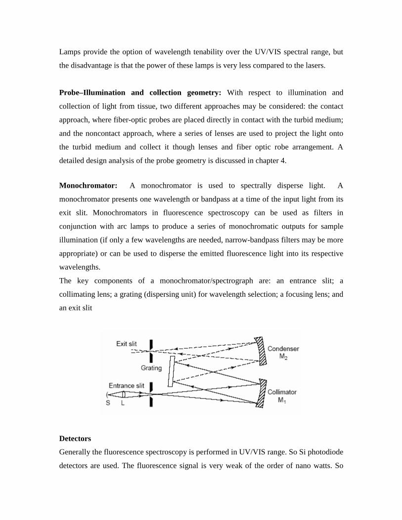
Monochromator: A monochromator is used to spectrally disperse light. A

monochromator presents one wavelength or bandpass at a time of the input light from its

exit slit. Monochromators in fluorescence spectroscopy can be used as filters in

conjunction with arc lamps to produce a series of monochromatic outputs for sample

illumination (if only a few wavelengths are needed, narrow-bandpass filters may be more

appropriate) or can be used to disperse the emitted fluorescence light into its respective

wavelengths.

The key components of a monochromator/spectrograph are: an entrance slit; a

collimating lens; a grating (dispersing unit) for wavelength selection; a focusing lens; and

an exit slit

Detectors

Generally the fluorescence spectroscopy is performed in UV/VIS range. So Si photodiode

detectors are used. The fluorescence signal is very weak of the order of nano watts. So

generally a photomultipler tube (PMT) is used in conjunction with Si photodiode

detector. Sometimes CCDs are also used for detection.

Chapter 2

Monte-Carlo model of light transport in turbid medi um

2.1 Monte Carlo Simulation

Monte Carlo Simulation is a powerful method that is used to solve various physical

problems by constructing a stochastic model in which the expected value of a certain

random variable or a combination of several variables is equivalent to the value of a

physical quantity to be determined. This expected value is then determined by the

average of multiple independent samples representing the random variable introduced

above. The random variable can be generated using different kind of distribution which

can be realized using programming techniques. Monte Carlo simulations thus offer a

flexible, yet rigorous approach to photon transport in a turbid solution: which can score

multiple physical quantities simultaneously. The method describes local rules, of photon

propagation that are expressed, in the simplest case, as probability distributions that

describe the step size of photon movement between sites of photon-particle interaction in

the medium, and the angles of deflection in a photon’s trajectory when a scattering event

occurs. However, the method is statistical in nature and as such, relies on calculating the

propagation of a large number of photons (e.g.50 000) by the computer.

2.2 Modeling the Laser Source

The initial task in hand was to simulate the output of a laser source. As evident the laser

light has a Gaussian profile. This was simulated by making the photons to be emitted out

of the fiber core with a radial distribution given by the a Gaussian probability function

shown below-

P(r) = (1/ σ√ 2π) Exp (-r2/2σ2)

However, the fibers that we were using produced multiple modes. Hence it was estimated

that the laser light profile given by a Super-Gaussian distribution will prove to give a

better solution. The super Gaussian distribution function is given by the following

equation.

P(r) = C Exp (-r4/2)

where C is the normalized constant. The above equation is for a variance of 1 unit.

However a random number with the required variance can be achieved by simply

multiplying the random number generated using the equation above, by the required

variance. Generating a random number with a Super-Gaussian distribution involved a bit

of tedious work as it requires developing a time efficient algorithm. Unlike other standard

distributions like the Gaussian, which is a built-in-function in the Matlab directories,

there is no provision for generating Super-Gaussian random numbers.

Generation of Super-Gaussian Random Numbers

The basic steps involved in the generation of Super-Gaussian random number are-

1. To choose randomly (Uniform distribution) a value of r that lies inside the core of

a fiber i.e. 0 to core radius.

2. Calculate the value of the super Gaussian distribution at r (normalization constant

C=1) and store it in a variable f.

3. Next generate a new uniformly distributed random number between 0 and 1 and

store its value in y. If the value of the variable y is less than the f then r is chosen

else it is discarded.

4. On performing the above steps large number of time we get the values of r that

follow a super Gaussian distribution.

2.3 Simulation model for scattering and absorption process

Light transport can be modeled by two different methods- weighted approach or now

weighted approach [1]. In weighted approach, after each propagation step, a part of the

packet is absorbed and a part is scattered. But in non–weighted approach, either the

whole photon packet is absorbed or scattered i.e., each photon packet is being considered

as a single photon. The weighted approach gives a good accuracy over non-weighted

approach. So in all our modeling we considered weighted approach.

The scattering process is modeled using the Monte Carlo Techniques based on variable

step size method. The steps involved are-

Figure 1: Flowchart for the variable stepsize Monte Carlo technique.

2.3.1 Photon Initialization

The simulation is performed for a fixed number of photon packets that are made to emit

randomly from the central fiber of the optrode. The modeling is done by considering one

Launch New Photon Packet with intial weight wi

Move distance s

Absorb

−= −

t

aii µ

µωω 11

Scatter (Using Henyey-Greenstein

function)

Photon Collected by

detector

Pi = Pi-1 + wi

wi < wcritical

Yes

No

Yes

No

End

Last Photon

photon packet at a time. The weight of the photon packet is initialized to one. A point is

randomly chosen on the fiber (r,Ψ) which is obtained by generating a Super-Gaussian

random number r and a uniformly distributed random number phi. Next the photon

direction is randomly chosen within the numerical aperture of the fiber. The direction

cosines of the photon are stored using variables (ux, uy, uz).

2.3.2 Generating propagating distance

The step size of the photon packet is calculated based on a sampling of the probability

distribution for the photon’s free path s (0 < s < ∞), which is the step size. According to

the definition of interaction coefficient µt, the probability of photon-particle interaction

per unit path length in the interval (s’, s’ + ds’) is:

or

where P{} gives the probability for the condition inside the {} to hold The above

equation can be integrated over s’ in the range (0,s1) and can lead to an exponential

distribution, where P{s ≥ 0} = 1 is used:

The probability density function of free path s is:

On using the above equation the step size with the above exponential distribution can be

calculated to be

where ξ is a uniformly distributed random number between 0 and 1. Note that the average

of the random numbers generated above gives the mean free path of the photon-particle

interaction in the turbid medium.

The photon free path or the step size is estimated using the above exponential distribution.

A particular value of ut is thus chosen for performing the simulation. This distance is then

converted into the coordinate system by multiplying s with the direction cosines. After

moving a distance s, the position of the photon is updated.

2.3.3 Absorption

After each propagating step, the weight of the packet is split into two parts- the absorbed

part and the scattered part. The absorption of the photon packet is taken into account by

decreasing the weight of the photon packet according to the following equation:

2.3.4 Scattering Model

In this case the incident photons behave like a particle and interact with the atom of the

medium causing scattering. The process of scattering depends on the type of particle with

which the atoms interact. Depending on the medium, the photon scattering can either be

isotropic or anisotropic. According to the scattering model used by us, the anisotropy

term is expressed by a g-factor. The model assumes a diffused scattering with the cosine

of the scattering angle given by a probability distribution which is a function of the g

factor. The probability distribution for the cosine of the deflection angle, cosθ, is

described by the scattering function-

where the anisotropy factor g can have a value between -1 and 1. A value of 0 denotes

isotropic scattering, -1 as back scattering and 1 as forward scattering. Using the above

equation the value of cosθ as a function of a random number ξ (uniformly distributed

random number between 0 and 1) can be calculated to be-

−= −

t

aii µ

µωω 11

Steps during scattering

The remaining part of the photon packet left over after absorption undergoes scattering as

follows:

1. The scattering model as discussed above is used in identifying the scattering angle

of the photon (θ), which can lie in the range 0 to 180oC. The angle θ depends on

the g factor which can be chosen between -1 to 1. Again a particular value for g is

chosen for the simulation.

2. Along with the angle θ, a Ψ angle is also calculated. Ψ essentially helps in

realizing a 3D motion of the photons. It is clear that Ψ follows a uniform random

distribution and can have values between 0 and 360o.

3. Next the direction cosine of the photon is updated using the values of the

scattering angle θ and Ψ as obtained above.

4. This process (from step 3 to step 7) is repeated again and again till one of the

termination conditions is encountered. Different termination conditions are used

for handling two cases which is discussed in the next sections.

5. Once the termination condition is achieved a new photon is then incident into the

turbid medium and the above steps are repeated.

2.3.5 Termination Conditions:

Two cases are considered in evaluating the scattering parameter g and ut.. Both these

cases are realized using different termination conditions that are mentioned below-

Case 1: Termination Condition for Diffused Reflection

a. The photon after multiple scattering goes back into the collecting fiber.

This is done by monitoring the z value. If the z value becomes negative

then the position of the photon is calculated and compared with the probe

dimension.

b. If the photon moves forward beyond a critical distance, then the photon is

terminated. In this model we have assumed that once the photons cross a

critical distance Zcritical, chances that they scatter back and be collected is

minimal. Typical values choosen by us is about 10 cm which is quite

justifiable.

c. Also a radial limit is put on the motion of the photons i.e. if the photon

crosses a certain critical distance Rcritical then we terminate the loop and

discard the photons.

Case 2: Simulation Technique for Modeling Transmitted Light

a. The photon after multiple scattering goes back into the collecting fiber and

hence not detected. This is done by monitoring the z value. If the z value

becomes negative then photon is discarded and the loop terminated

b. If the photon moves forward beyond a distance, i.e. the point at which we

are detecting the photon (Detector). In such a case the photon is taken into

account and a new photon is then made to incident onto the medium.

c. A radial limit is put on the motion of the photons i.e. if the photon crosses

a certain critical distance Rcritical then we terminate the loop and discard the

photons.

2.4 Verification of the Program Code

In order to check the simulation, the incident

photons are made to fall on the medium and the

distribution of the photons scattered back on to the

fiber is plotted on a graph. In the first trial we

received a non-uniform pattern as can be seen in

Figure 3.1. This made us debug the program code,

until we received a uniform distribution of the back

scattered light. Figure 3.2 shows the distribution

obtained after the corrections, indicating that the

program code is working well and can be used for

simulating different working conditions. The empty

circle at the center is the illuminating fiber.

2.5 Simulation model for fluorescence

In the earlier model, photon on interaction with medium is either scattered or absorbed. In

the model for fluorescence, once the photons are absorbed by fluorescent medium, a new

photon at different wavelength is emitted.

The ‘g’, ‘µs’ and ‘µa’ for an incident photon and an emitted fluorescent photon are

different and their values have to be used accordingly. The important steps in the

simulation model are as follows:

Figure 3.1

Figure 3.2

1) For scoring photon absorption, a two-dimensional homogeneous grid system is set

up in the r and z directions. The grid separations are Ar and Az in the r and z

directions, respectively.

2) Photons from the illuminating fiber propagate through the medium experiencing

both scattering and absorption as per the model in 2.3. At each stage of absorption,

the weight of the photon packet that is absorbed is stored in the local grid element

(Ar i, Azi).

3) After all the photons are exhausted (say 1,00,000 photons) , the simulation for

fluorescence is executed. From each local grid element, photons are emitted

isotropically, which corresponds to the fluorescence signal. The number of

photons that are emitted from each grid element are equal to the closest integer to

the weight of the local grid element,

4) Once the fluorescence photon is emitted, the propagation steps are same as one in

section 2.4, except that the photon now travels with a different ‘g’, ‘µs’ and ‘µa’.

5) The terminations conditions are applied as per the probe design.

Chapter 3

Estimation of the optical properties of a turbid medium

Importance of finding the optical parameters

We started our project, performing experiments on the measurement of the diffused

reflection. The collected power was measured for different input powers. However,

simulation of the above experiment requires the values of the three parameters g , µs and

µa of the liquid. Using the above experiment, it is not feasible to determine all the above

interaction parameters. Thus, a new experiment had to be set up to identify these

parameters.

Before proceeding, it is important to understand some of the fundamental aspects of the

light-matter interaction. As was discussed in the last chapter, two mechanisms viz.

scattering and absorption occur when light interacts with a medium. The scattering

mechanism is characterized by the parameters g and µs. The g parameter depends on the

way the photon interacts with the atoms of the medium and hence is independent of the

concentration of the turbid medium. However, it depends on the size of the scattering

particles in the medium and is also a strong function of the wavelength. The absorption

mechanism on the other hand is characterized by the parameter µa. Both µa and µs depend

on the concentration of the medium i.e. if the medium is dense then the photons interact

with the particles at a much shorter distance (photon free path) and thus intensity drops

drastically. The sum of µa and µs gives us the total interaction coefficient denoted by µt.

Different experiments (as discussed below) were tried in an attempt to identify these

parameters for simulating the light propagation in a turbid medium.

Experiments for estimation of optical parameters

Commonly used methods

A lot of literature survey was done to identify such experiments. We came across two

most widely used methods. The most common method was the integrating sphere

technique.

Integrating sphere technique: The spectrophotometer measures direct transmission of

light through a sample as a function of wavelength. When equipped with an integrating

sphere attachment, the spectrophotometer can also measure the diffuse reflection and

total transmission of a sample. Three different measurements (collimated transmission,

diifuse transmission and diffuse reflection) are therefore available as a function of

wavelength.

Once these measurements are done, then simulations are used to determine the optical

parameters. The most common simulation code is the inverse-adding doubling method [].

experiments.

The drawback of the method is that most

commonly available spectrophotomters does

not have integrating sphere attachment for

liquid samples; the attachment is generally

provided only for thin films.

1) Diffused reflectance

When the hole is (not) closed, detector gives (diffused transmittance.. (2)) total transmittance

Total - diffused gives

collimated transmittance.(3)

The other drawback is that, even if such an arrangement was set-up for liquid samples,

then there will be significant losses of light from the side walls of the liquid container (as

shown in fig.), which will lead to errors in the estimated optical parameters. In our

method, these losses are eliminated.

The other method that can be used for estimation of the optical parameters is by time

resolved spectroscopy analysis. However, it is expensive and a complex set-up.

Experimental methods developed by us

As the existing methods were difficult to implement, we were left to explore a new and

simple way of identifying the parameters. As a first attempt, we neglected the

contribution due to the absorption by the liquid i.e. µa = 0; µt = µs. This simplified our

problem to a two variables problem viz g and µs.

I. Method for pure scattering case

To determine the scattering

parameters a new experiment was

designed. This involved the

measurement of the Diffused

Transmittance for different

apertures. Fig.1 shows the

experimental set-up. Here a laser

beam was coupled to the fiber from

one end. The other end of the fiber

was mounted on an XYZ translator stage with its tip inserted into the turbid medium. The

turbid medium was placed in a cylindrical glass cell with a flat bottom; the cell was

constructed by fixing a glass cover- slip at one end of a small glass cylinder. A variable

aperture followed by a detector was placed just below the cell. The transmitted power for

different apertures was measured at different value of ‘z’. Optical alignment and

Detector

MO

Power meter Turbid

solution z

He-Ne Laser (543 nm)

Fig. 1: Set-up for diffused transmission experiment

Variable Aperture

zx

y

positioning of the fiber tip with the aperture and the detector was achieved using X-Y

translation.

Fig 2 shows the

normalized output for

two different

concentrations of

turbidity. Using Fig.2

the intensity drop was

measured at a distance

Z=0.3mm for each

aperture values.

Aperture 4 and aperture

5 give similar readings.

Also due to error in

experiment aperture 1 is

neglected. The radius

for the three apertures

(2, 3 & 4) is – 325µm,

655µm & 1035µm

respectively. Also a rough

estimate of 8% loss in the

collected power due to

the glass slide was

observed while

performing the

experiment. Hence, in an

attempt to match the

experimental results with

the simulation, an 8%

increase is made to the

Table 1: Collected no of photons for 30000 incident photons

25% turbidity

0

0.2

0.4

0.6

0.8

1

1.2

0 100 200 300 400 500 600 700 800

Distance(Z in micormeter)

Po

wer

e(N

orm

aliz

ed t

o 1

)

aperture2

aperture3

aperture4

aperture5

50% turbidity

0

0.2

0.4

0.6

0.8

1

1.2

0 50 100 150 200 250 300 350 400 450 500

Distance (Z in micrometer)

Po

wer

( N

orm

aliz

ed t

o 1

)

aperture1

aperture2

aperture3

aperture4

aperture5

Fig 2: Normalized Collected Power at different Z for two different turbidity

collected powers, expressed in no of photons collected for 30000 incident photons. To

find out g and µt we had adopted the following method-

The experimental ratio of output to input power at a particular distance ‘Z ‘ was noted for

different apertures and compared it with the ratio obtained by simulation (output number

of photons to the input number of photons at the same ‘Z’ for the corresponding

apertures). Table 1 shows the observed results for Z = 0.3mm for three apertures namely

2, 3 and 4.

Next for each aperture, the

possible values of ‘g’ and ‘µt’

were noted from the simulation

results and plotted in Fig 3. The

curves for different apertures

intersect at a particular value of ‘g’

and ‘µt’, because of the fact that,

for a given turbidity ‘g’ and ‘µt’

remains same. From Fig. 3, we

notice that the curves intersect at a

common point around g = 0.9 & M.F.P (mean free path = 1/ µt) = 77nm. However,

simulations at such low values of M.F.P were not completely performed as it requires

large computational time. Hence we need to confirm the results by performing

simulations for lower M.F.P‘s as well.

With these calculations we are able to estimate our parameters ‘g’ and ‘µs’ qualitatively.

But the arrangement for the above setup esp. alignment of the aperture with the detector

was tedious and time consuming.

Now with an idea of the above method we tried to move to a three variable problem.

Another experiment on Collimated transmission was setup and few minor changes were

-1.0 -0.8 -0.6 -0.4 -0.2 0.0 0.2 0.4 0.6 0.8 1.0

02468

101214161820222426283032343638

Pho

ton

Mea

n F

ree

Pat

h(M

.F.P

)- u

m

g

Aperture 2 Aperture 3 Aperture 4

Fig 3: Plot of M.F.P Vs g for different Apertures

made to the existing Diffused transmission experiment for estimating the parameters ‘g’,

‘µa’ and ‘µs’.

II. Collimated Transmission experiment

Collimated transmission experiment

was setup to identify the total

scattering coefficient ut. A green He-Ne

(543 nm) laser beam was made to pass

through a certain length of the turbid

liquid placed in the wedge (Fig.4) and

the collimated light was measured

using a photo detector placed far away from the sample to ensure that no scattered power

was collected. The measured power was normalized with a reference liquid, usually water

or the solvent with which the turbid solution was prepared. The experiment was

performed for different sample lengths by moving the cell across the laser beam and the

average value of µt was calculated.

III. Method by considering both scattering and absorption mechanism

The three parameters ‘g’, ‘µa’ and

‘µs’ could also be written in a new

form as ‘µt’ , ‘g’ and ‘b’. A term

‘albedo’ denoted by b is introduced

which is defined as the fraction of

light getting scattered and is

expressed as.

t

sbµµ

=

The value of µt is measured using the

collimated transmission experiment. An advantage of writing the original parameters to

Power meter

Detector

He-Ne Laser (543 nm) MO

Turbid solution z

x

y

z

Fig. 5: Set-up for diffused transmission experiment

Power meter

He-Ne Laser (543 nm)

Turbid solution in a fabricated cell

Scattered Light

Fig. 4: Set-up for collimated transmission experiment

Milk (g=0.91, b = 0.865)

0.8

0.85

0.9

0.95

1

1.05

0.7 0.75 0.8 0.85 0.9 0.95 1

g

alb

edo

(b)

z=6mm

z=9mm

z=12mm

0.91

new form is that both the parameters ‘b’ and ‘g’ can have values between 0 and 1 only.

This makes the simulation analysis much easier. These two parameters were obtained

using the diffused transmission setup (Fig 5). In this setup, the aperture was removed and

the detector of a known active area was placed directly below the cell. The transmitted

power for different values of z was measured.

The ‘diffused

transmission’

power collected

by the detector

was measured

for three

different values

of z and was

normalized with

respect to the

corresponding

power, when the

turbid liquid was replaced by

the reference sample (DI water or the solvent with which the turbid medium was

prepared). A Monte Carlo simulation was developed with the above measured value of µt

and values of g and b between 0 and 1 were used as an input. Using the Monte Carlo

simulation (discussed in chapter 2), we determined the corresponding power collected

within the aperture of radius R. For each value of z, the experimentally measured

normalized power was matched with the simulation result for several possible

combinations of b and g. Figure 6 shows the three curves, corresponding to the three

different values of z, representing the possible combinations (g,b). For a given turbid

medium, since the optical properties are constant and are independent of the choice of z,

the common point of intersection give us the values of b and g for that liquid.

Fig. 6: Plot of (g,b) for different values of z (6mm, 9mm ,&12mm)

Results:

Experiments on milk

Experiments were performed on milk (1 ml milk in 40ml water) and the results were

parametric optimized with the simulation. The possible pairs of (g ,b) for each z are

identified and plotted in figure 3. The curves intersect at a common point g=0.93, b=0.87.

The results for g were in agreement with I.V. Yaroslavsky et al [4], which gives a good

confirmation of our method.

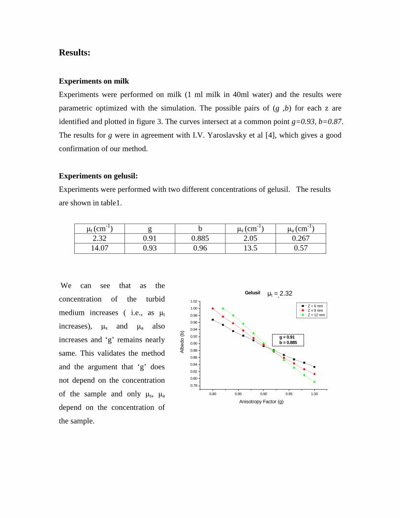
Experiments on gelusil:

Experiments were performed with two different concentrations of gelusil. The results

are shown in table1.

We can see that as the

concentration of the turbid

medium increases ( i.e., as µt

increases), µs and µa also

increases and ‘g’ remains nearly

same. This validates the method

and the argument that ‘g’ does

not depend on the concentration

of the sample and only µs, µa

depend on the concentration of

the sample.

µt (cm-1) g b µs (cm-1) µa (cm-1) 2.32 0.91 0.885 2.05 0.267 14.07 0.93 0.96 13.5 0.57

0.80 0.85 0.90 0.95 1.00

0.78

0.80

0.82

0.84

0.86

0.88

0.90

0.92

0.94

0.96

0.98

1.00

1.02

g = 0.91b = 0.885

Gelusil

Z = 6 mm Z = 9 mm Z = 12 mm

Alb

edo

(b)

Anisotropy Factor (g)

µt = 2.32 cm-1

Experiments on Ag nanoparticles

For both milk and gelusil, the ‘g’ factor was more than 0.9. In order to check the theoretical argument that ‘g’ factor depends on the dimensions of the scattering particles, we have performed experiments on silver nanoparticles. These nanoparticles have dimension much less than the wavelength of the laser light, so theoretically the scattered light should be more isotropic compared to the case when the dimensions of the scattering particles are of the same size as that of wavelength. The silver nanoparticles that we used in our experiment were borrowed from thin film lab, and their was around ~150 nm as estimated from SEM.

From the above graph, we can see that the ‘g’ factor for silver nanoparticles is around 0.65 and this validates the method and the argument that ‘g’ factor depends on the dimensions of the scattering particles.

Silver nanoparticles

0.4

0.5

0.6

0.7

0.8

0.9

1

1.1

0.3 0.35 0.4 0.45 0.5 0.55 0.6 0.65 0.7 0.75 0.8 0.85 0.9 0.95 1

g

Alb

edo

(b

)

z =3mm

z =6mm

z =9mm

Chapter 4

Probe Design Analysis

There are several issues involved in designing an optimum probe for collecting

fluorescence signal. The foremost issue is the probe size i.e. how big should the probe be

and under what circumstances could it be used? For e.g if we need to use designing a

probe for endoscopy, then we need to consider the probe size as the deciding factor for

fabrication rather than on improving the signal at the cost of a larger probe. In endoscopy,

we have a bundle of fibers, with one or few fibers as the illumination centers and the rest

serving as the collection centers. The collection efficiency is improved by the use of a

ball lens, but however the collection of the fluorescence signal is limited by the small

numerical aperture of the fiber. Thus only a small fraction of the fluorescence signal gets

coupled to the collecting fibers.

But if there are no size constraints then we can design a probe whereby the collection

efficiency can be improved by using a lens system that can couple more fluorescence

signal to the fiber. In this project, we have tried to perform experiments on fluorescence

and determine the possible optimized probe geometries. There are two ways in which the

probe could be designed - (1) In proximity mode or (2) remote mode (optrode not in

contact with the liquid).

Proximity Mode

In continuation to our work before the mid-semester evaluation, we have tried to study

the light propagation through fluorescence liquid (Rhodamine 6G and Basonyl Rot 542)

and tried to calculate the expected signals for different configurations of the probe. In the

proximity mode, the optrode was kept very close to the liquid. Rhodamine 6G has an

absorption maximum at 529.5nm and fluorescence excitation peak at 556nm. Basonyl

Rot has an absorption maximum at 542nm and an excitation peak at 600nm. For the He-

Ne laser source at 543nm, Basonyl Rot 542 gives a stronger signal as compared to

Rhodamine 6G and thus was preferred for experimental purposes.

The different configurations tried are listed below:

1. Simple geometry – In this case the probe was simply immersed in a liquid and

simulation analysis was done to calculate the measured signal (Fig 1). Experiment

was also performed for this configuration and the following plot was obtained.

2. Concave Reflector- In this case a concave reflector was placed inside the turbid

medium as shown in Fig 4.2. A Monte Carlo model simulating such an

experimental setup was developed with two input parameters L, distance between

the immersed optrode tip and the center of the concave mirror and R, radius of

curvature of the mirror. Fig 4.3 shows the variation of the fluorescent signal for

different values of R for a given L. The experiment was performed for three

Figure 4.2: Experimental Setup with a simple probe geometry

Power meter

Detector Laser

MO

Fiber chuck

Turbid solution

Figure 4.1: Experimental Setup with a simple probe geometry

Power meter

Detector Laser

MO

Fiber chuck

Turbid solution

different values of L. The x- axis is shown in terms of the ratio R/L rather that R.

We notice that the signal is strongest when the ration R/L lies between 1.4-1.7.

Thus it is appropriate to take the R/L ratio to be 1.5 as the optimized condition for

efficient collection of the fluorescent signal. i.e. L = 2R/3.

R,L Optimization Chart

0

0.1

0.2

0.3

0.4

0.5

0.6

1 1.2 1.4 1.6 1.8 2 2.2 2.4

Ratio of R/L

Flu

ore

scen

t sig

nal

( in

% o

f in

cid

ent

ligh

t)

L=3mmL=5mmL=4mm

Next the length L was varied to measure the optimum L so that maximum

fluorescence signal was obtained. Fig 4.4 shows that plot indicating that for the

given liquid with the interaction parameters (‘g’=0.9, ‘µs’=2, ‘µa’=3 ), maximum

signal was collected when L = 2.5mm.

3. Concave Reflector with a Condenser Lens: A lens was added to the previous

setup and collected signal was calculated for L=2R/3. Simulation was developed

for this experiment. The output of the simulation yields the results in Fig 4.5. An

Figure 4.4: Fluorescent Signal Vs L for R/L=3/2

Figure 4.3: Fluorescent Signal Vs R/L ratio

0

0.1

0.2

0.3

0.4

0.5

0.6

0 1000 2000 3000 4000 5000 6000 7000 8000 9000 10000

Distance(L)

Flu

ore

scen

ce s

ign

al (i

n %

of t

he

inci

den

t lig

ht)

increase in the signal was obtained for 2 different values of the focal length i.e.

3cm and 6cm of the condenser lens (Bi-convex lens).

Based on the above experiments we got a good idea of some aspects that are discussed

below-

• The fluorescence signal collected by the optrode is restricted to only few

millimeter of the liquid length i.e. majority of the signal collected by the optrode

is within 2-3 mm of the liquid length below the optrode tip.

• Large amount of the fluorescence signal backscattered went into the illuminating

fiber which meant only small amount of power was collected by the collecting

fibers.

Figure 4.5: Fluorescent Signal Vs Focal Length of the Condenser (Biconvex) Lens for L=2500. R/L=3/2

Power meter

Detector Laser

MO

Fiber chuck

Turbid solution

Condenser Lens

Figure 4.4: Experimental Setup with a probe having reflector and lens system geometry

Optimized Bi-convex Lens

0.25

0.27

0.29

0.31

0.33

0.35

0.37

0 1 2 3 4 5 6 7 8 9

Focal Length (cm)

Flu

ore

scn

et s

ign

al (

in %

of

Inci

den

t L

igh

t)

• Since the reflector also needs to be placed within 2-3 mm, this requires us to use a

condenser with a high N.A so that illuminating signal focuses to the central region

between the condenser and the mirror.

Thus based on the above observations it was decided to use the configuration shown in

Fig 4.6. for the contact mode. Here we have two illuminating fibers at the side. The light

from these fibers are focused to a spot at the center in the liquid, using a high N.A

condenser (or Microscope objective). The collecting fibers are placed at the center of the

system. Such a configuration helps us to overcome the limitation seen in the earlier

experiments i.e. the fluorescence collected at the center of the optrode is also carried with

the other collecting fibers.

But the major factors limiting these configurations are that (a) the fiber N.A is small and

so only a very small fraction of the fluorescence signal is coupled to the fibers and (b)

due to finite focal length of the liquid, the fluorescent signal is reabsorbed as it

propagates through the liquid towards the collecting fiber. At this stage we came up with

an innovative idea of doing an N.A down-conversion which is explained in the remote

mode.

Remote Mode

In this case the optrode is placed at a distance from the liquid medium. The fluorescence

from the liquid is then collected using a lens system, aiding N.A down-conversion. Some

ideas were taken from the experimental setup on Laser Doppler Anemometry. The liquid

sample is placed in a capillary tube and the illuminating light is focused onto the tube

(see Fig 4.7). A line streak is formed as the light passes through the capillary. The lens

system is such that this line streak is collimated using a higher N.A. lens, which then is

focused onto the collecting fibers using another lens with a N.A same as that of the fiber.

An experiment was setup with the above concept. Such a N.A down-conversion system

(see Fig 4.8) gives a better signal and was found to yield higher signal strength than the

proximity case.

Since there is no restriction on the size of the probe, we have decided to use this approach

in designing the final probe. We also plan to use a reflector so that a larger fraction of the

fluorescence signal is coupled to the optrode.

Optrode Fiber N.A = 0.22

(Hemi-)Spherical Mirror

Fluorescent Sample (Line Streak)

Bi-convex lens (N.A = 0.7)

Bi-convex lens (N.A = 0.22)

Figure 4.8: N.A. Down-conversion using a lens system

Fabrication of optrode: The final design of the probe that was fabricated is as shown in the figure:

The important parts of the design are

1) Main tube

2) Illuminating arrangement

3) Capillary tube that holds the liquid sample

4) Collecting lens arrangement

5) Collecting optrode

Main tube:

The tube is made of PVC and it holds all the arrangements in it viz, illuminating and

collecting lens arrangements, capillary tube and collecting optrode.

Collecting optrode (5)

Main tube

Lens Mirror Small capillary tube

High NA Lens

Low NA Lens

Illuminating arrangement (2)

Collecting lens arrangement (4) Capillary

tube (3)

Illuminating arrangement:

The illumination arrangement consists of an illuminating fiber, a mirror and a lens. The

laser was coupled to one end of the illuminating fiber and the other end was passed

through a capillary tube (with a very small bore), which provides support for the fiber.

The light from this fiber end falls on mirror placed at 450 to the axis of the main tube.

The reflected light is then made to pass through a lens (focal length of 12.5 mm), which

focuses light on capillary tube.

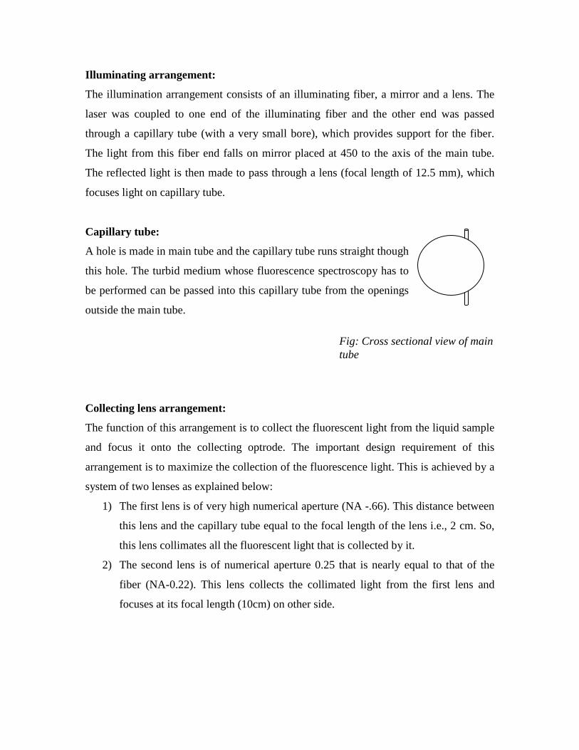
Capillary tube:

A hole is made in main tube and the capillary tube runs straight though

this hole. The turbid medium whose fluorescence spectroscopy has to

be performed can be passed into this capillary tube from the openings

outside the main tube.

Collecting lens arrangement:

The function of this arrangement is to collect the fluorescent light from the liquid sample

and focus it onto the collecting optrode. The important design requirement of this

arrangement is to maximize the collection of the fluorescence light. This is achieved by a

system of two lenses as explained below:

1) The first lens is of very high numerical aperture (NA -.66). This distance between

this lens and the capillary tube equal to the focal length of the lens i.e., 2 cm. So,

this lens collimates all the fluorescent light that is collected by it.

2) The second lens is of numerical aperture 0.25 that is nearly equal to that of the

fiber (NA-0.22). This lens collects the collimated light from the first lens and

focuses at its focal length (10cm) on other side.

Fig: Cross sectional view of main tube

Collecting optrode:

The collecting optrode is a bundle of fibers that carries the fluorescent light to the

detector. The geometry of the fiber bundle has to be such that it collects the maximum

fluorescence light.

Because the incident light on the capillary tube is line streak, we find that the collected

fluorescence light is also a line of streak. So the best possible arrangement of the

collecting optrode is linear array of fibers. However, as we have already fabricated a

optrode with hexagonal arrangement of fibers, in all our initial experiments we have used

this circular optrode.

The important steps in the fabrication of the collecting optrode are as follows:

• The dimensions of the fibers used are as follows:

Core (silica) – 600µm

Cladding (silica) - 660µm

Jacket (silica) - 710µm

Numerical Aperture -0.22

• The optrode consists of three layers of fibers (1-6-12)

• The 19 fibers were cut from the spool, each one with a length of around 1m. All

the fibers were passed through short individual pieces of sleeves, so that these

fibers don’t break by getting stressed against the glass bore, into which the fibers

were inserted.

• Now to get the arrangement of 1-6-12 fibers, the fibers were simply placed

together and then a thread was tied from the position where the sleeves were

located and continued towards the end, so that the fibers automatically get into the

required hexagonal arrangement. The fibers were permanently held in this

arrangement by using an adhesive.

• The fibers are then passed through a short glass bore and the fiber arrangement is

held in place with respect to the glass bore by putting wax (Beeswax + rosin is

melted and introduced into the gap, which on cooling solidifies)

Adhesive

Arranging the fibers in hexagonal pattern

Outer glass bore Teflon

tape

Sleeve

Cross Section

• All these fibers are now passed through a second glass

bore of bigger size, so that the position of the sleeves

matches with the edge of the bore. A Teflon tape is

used at the end where the sleeves are present to ensure

that the fiber and the glass bore are held together. The

gap between the opening end of the first bore and the

second bore is again filled with wax.

• Rough grinding and polishing: Unlike the normal fibers,

these fibers cannot be spliced easily to get a circular cut,

because they are very brittle. So it is necessary to grind

and polish to get smooth ends. It is also necessary that

the surfaces of the polished fiber ends should be flat,

without formation of any wedges. So a disc with hole

was fabricated from the workshop. This disc is now

fixed to the end of the optrode. The grinding Figure 6.2: Arrangement for grinding and polishing

Glass slab

Figure 6.1: Fabrication of optrode

was then done with emery (aluminum oxide) of different grades - MA-1, MA-2,

and MA-3. As we increase the grade of the emery, the surface roughness is

reduced. Then polishing was done with a lapping agent and a velvet cloth as

polisher. The surface of the fiber end is checked under microscope and polishing

is continued until the pit size is considerably reduced.

• After one end of the optrode is polished, similar steps of arranging the fibers in a

glass bore and polishing were performed with the other end.

Chapter 6

Conclusion and Future Plan

6.1 Conclusion

• A Monte-Carlo simulation incorporating all three mechanism-scattering,

absorption and fluorescence is developed.

• A simple and novel method to determine the optical properties ‘b’ and ‘g’ of a

turbid solution is developed. The method gives a straightforward estimation of the

optical properties for any turbid medium containing both scattering and absorbing

particles. One of the advantages of this method is that the model can be used to

calculate the effective anisotropy coefficient g of a turbid medium containing

more than one kind of scattering particles. This effective value of g can then be

used to study the light propagation in the given medium.

• Different designs for the optrode have been studied.

6.2 Future Work

• For determination of optical parameters, further experiments are required to

improve the accuracy. Some of the changes to made in simulation are to

incorporate reflections losses at glass slide. Experiments with latex spheres

(whose size is already known from the suppliers) for determination of optical

properties will help in further improvement of the procedure.

• Many designs can be fabricated and studied based on our proposed designs

mentioned in chapter 4. By theoretically analysis (ray approach) it can be said that

using reflectors and lenses will improve the collection efficiency. But a lot of

simulation analysis is needed to find out the optimum dimensions of these

reflectors and lenses. So all the future Monte Carlo simulations should have the

provision for incorporating these components.

• One of the limitations during the project was to find out a monochromator with

good resolution and a filter to separate the input laser signal from fluorescence

signal. Once a good filter and monochromator are found, several new designs can

be tried (using ball lens) which might be very compact and similar to the optrodes

used for endoscopy applications.

References

1) Characteristics of a high-temperature fibre-optic sensor probe Z.Y. Zhang,

K.T.V. Grattan *, A.W. Palmer, B.T. Meggitt, Sensors and Actuators A 64

(1998) 231-236

2) Fiber Optic Probes in Optical Spectroscopy, Clinical Applications

3) Multiple-fiber probe design for fluorescence spectroscopy in tissue, T. Joshua

Pfefer, Kevin T. Schomacker, Marwood N. Ediger, and Norman S. Nishioka,

APPLIED OPTICS _ Vol. 41, No. 22 _ 1 August 2002, 4712-4721

4) Light Propagation in Tissue During Fluorescence Spectroscopy With Single-

Fiber Probes, T. Joshua Pfefer, Kevin T. Schomacker, Marwood N. Ediger, and

Norman S. Nishioka, IEEE JOURNAL ON SELECTED TOPICS IN QUANTUM

ELECTRONICS, VOL. 7, NO. 6, NOVEMBER/DECEMBER 2001, 1004-1012

5) Influence of the emission–reception geometry in laser-induced fluorescence

spectra from turbid media, Sigrid Avrillier, Eric Tinet, Dominique Ettori, Jean-

Michel Tualle, and Bernard Ge´ le´ bart, 1 May 1998 y Vol. 37, No. 13 y

APPLIED OPTICS, 2781-2787

6) Fiber-optic bundle design for quantitative fluorescence measurement from

tissue Brian W. Pogue and Gregory Burke, 1 November 1998 y Vol. 37, No. 31

y APPLIED OPTICS, 7429-7436

7) Optical fiber probes for fluorescence based oxygen sensing P.A.S. Jorge a,b,∗,

P. Caldas a,b,c, C.C. Rosa a,b, A.G. Oliva d, J.L. Santos, Sensors and Actuators

B 103 (2004) 290–299

8) An optimized optrode for continuous potassium monitoring in whole blood E.

Malavolti a, A. Cagnini a, G. Caputo b, L. Della Ciana b, M. Mascini Analytica

Chimica Acta 401 (1999) 129–136

9) L. Wang, S. L. Jacques, L. Zhenq, “MCML - Monte Carlo modeling of light transport

in multi-layered tissues”, Computer Methods and Programs in Biomedicine, vol. 47,

pp.131-146, 1995.

10) Accelerated Monte Carlo models to simulate fluorescence spectra from layered

tissues, Swartling et al., 714-727

11) Propagation of Fluorescent Light, A.J. Welch, PhD,* Craig Gardner, PhD,

Rebecca Richards-Kortum, PhD, Eric Chan, MS, Glen Criswell, BS, Josh

Pfefer, MS, and Steve Warren, PhD, Lasers in Surgery and Medicine 21:166–

178 (1997)

12) http://www.pti-nj.com/fluorescence_2.html

13) Noninvasive measurement of fluorophore concentration in turbid media with a

simple fluorescence_reflectance ratio technique, Robert Weersink, Michael S.

Patterson, Kevin Diamond, Shawna Silver, and Neil Padgett, 1 December 2001

_ Vol. 40, No. 34 _ APPLIED OPTICS, 6389-6395