design and characterization of optical metamaterials using
TRANSCRIPT

Air Force Institute of TechnologyAFIT Scholar
Theses and Dissertations Student Graduate Works
12-14-2012
Design and Characterization of OpticalMetamaterials Using Tunable PolarimetricScatterometryJason C. Vap
Follow this and additional works at: https://scholar.afit.edu/etd
This Dissertation is brought to you for free and open access by the Student Graduate Works at AFIT Scholar. It has been accepted for inclusion inTheses and Dissertations by an authorized administrator of AFIT Scholar. For more information, please contact [email protected].
Recommended CitationVap, Jason C., "Design and Characterization of Optical Metamaterials Using Tunable Polarimetric Scatterometry" (2012). Theses andDissertations. 949.https://scholar.afit.edu/etd/949

DESIGN AND CHARACTERIZATION OF OPTICAL METAMATERIALS USING TUNABLE POLARIMETRIC SCATTEROMETRY
DISSERTATION
Jason C. Vap, Major, USAF
AFIT-ENP-DS-12-03
DEPARTMENT OF THE AIR FORCE
AIR UNIVERSITY
AIR FORCE INSTITUTE OF TECHNOLOGY
Wright-Patterson Air Force Base, Ohio
APPROVED FOR PUBLIC RELEASE; DISTRIBUTION UNLIMITED

The views expressed in this dissertation are those of the author and do not reflect the official policy or position of the United States Air Force, Department of Defense, or the United States Government.

AFIT-ENP-DS-12-03
DESIGN AND CHARACTERIZATION OF OPTICAL METAMATERIALS USING TUNABLE POLARIMETRIC SCATTEROMETRY
DISSERTATION
Presented to the Faculty
Department of Electrical Engineering
Graduate School of Engineering and Management
Air Force Institute of Technology
Air University
Air Education and Training Command
In Partial Fulfillment of the Requirements for the
Degree of Doctor of Philosophy in Electrical Engineering
Jason C. Vap, B.S.E.E., M.S.E.E
Major, USAF
December 2012
APPROVED FOR PUBLIC RELEASE; DISTRIBUTION UNLIMITED


AFIT-ENP-DS-12-03
iv
ABSTRACT
Optical metamaterials are a class of engineered materials with a wide range of
material properties and an equally wide range of anticipated applications. These materials
traditionally attain their unique material properties from unit cell structures or material
layers which are periodically arranged. These periodic structures are often described
using effective medium theory (EMT), which is believed to remain valid so long as the
EMT description of the material is applied under long wavelength conditions (i.e. where
the incident wavelength can be assumed much larger than the unit cell or period
dimensions). This condition is increasingly difficult to achieve at optical wavelengths.
This problem was singled-out for negative refractive index materials, but they are not the
only optical metamaterial violating these dimensional constraints. One of the simplest
optical metamaterial structures was also found to be violating these constraints - a
periodic layered metal-dielectric structure used to attain near-zero permittivity at a visible
wavelength. In this research, a set of four periodic near-zero permittivity structures was
developed. A transfer matrix method (TMM) model was found to accurately predict the
experimental behavior of these structures but EMT did not. Additional modeling work
was completed to demonstrate the dimensional constraints necessary for EMT predictions
to match the predictions of a trusted and verified TMM model and establish a foundation
for future near-zero permittivity designs.
Of additional concern in metamaterials research, theoretical predictions for
metamaterials have been shown to have incident angle and incident polarization state
dependencies. Furthermore, these properties are narrow-band in nature. To date, optical

AFIT-ENP-DS-12-03
v
metamaterials have not been subjected to full-directional, full-polarimetric
characterization because there has yet to be an instrument developed with the spectral
range and full-directional, full-polarimetric capabilities needed to carry out this work.
This research work also addressed the instrument/characterization void in optical
metamaterials research. A tunable infrared (IR) Mueller matrix (Mm) polarimeter-
scatterometer was developed and operates with a fully optimized dual-rotating retarder
having 1/3 wavelength achromatic retarders.
After developing this instrument, it was used to measure the polarimetric behavior
of an infrared metamaterial absorber (MMA) at 5.0µm. This is the first spectral, fully
polarimetric and fully directional characterization reported for an optical metamaterial.
The extracted Mm for this sample was found to have incident angle dependence which
did not follow isotropic or anisotropic Fresnel reflectance behavior. However, the
experimentally retrieved Mm is valid and was used to predict the reflected polarimetric
behavior of the MMA when canonical polarization states were assumed incident on the
material.

1
ACKNOWLEDGMENTS
I would like to thank my family for their immense amount of support throughout
this research work. My love for you guys is truly without bound. I would like to thank my research advisor for his tireless support over the duration
of this research, particularly in these closing months. You have forever changed another mind.
I would like to thank our post doc for his commitment to our research and his
friendship over the last couple of years. You have been a great friend, and my family and I are grateful for having the opportunity to get to know you.
In closing, I would also like to thank my committee members for taking the time
out of their busy research and teaching schedules to be a part of my committee.
Jason C. Vap

2
TABLE OF CONTENTS
Page
Abstract .............................................................................................................................. iv
Acknowledgments................................................................................................................1
Table of Contents .................................................................................................................2
List of Figures ......................................................................................................................6
List of Tables .....................................................................................................................11
DESIGN AND CHARACTERIZATION OF OPTICAL METAMATERIALS USING TUNABLE POLARIMETRIC SCATTEROMETRY .......................................................12
I. Introduction ....................................................................................................................12
1.1 Optical Metamaterials and Effective Media ...........................................................12 1.2 Problem Statements .................................................................................................13
1.2.1 Validating the Use of Effective Medium Theory ............................................13 1.2.2 Instrument Demand for Infrared Metamaterials Research ..............................13
1.3 Research Objectives ................................................................................................14 1.4 Research Objective Accomplishment .....................................................................15
1.4.1 EMT use in periodic metal-dielectric near-zero permittivity designs .............15 1.4.2 Development of an IR Mm Polarimeter Scatterometer ...................................15 1.4.3 Measuring and Modeling an IR Metamaterial ................................................16
1.5 Organization ............................................................................................................16
II. Background ...................................................................................................................18
2.1 Near-Zero Permittivity Structures ...........................................................................18 2.2 Dual Rotating Retarder Optimization .....................................................................22
2.2.1 Discussion of the optimization problem .........................................................23 2.2.2 The unique optimization solution – random error analysis .............................24
2.3 Tunable Infrared Mueller-matrix Polarimeter-Scatterometer .................................24 2.3.1 Complete Angle Scatter Instrument ................................................................25 2.3.2 Practical design considerations .......................................................................26
2.4 Mm Measurements and Modeling of Novel Metamaterial Absorber .....................28 2.4.1 The Stokes Vector and its Poincaré Sphere Representation ...........................29
2.5 Conclusion ..............................................................................................................31
III. Modeling, Design and Experimental Analysis of Near-Zero Permittivity Structures at Optical Wavelengths ..........................................................................................................32
3.1 Executive Summary of Research ............................................................................32
3
Page
3.2 Introduction .............................................................................................................33 3.3 Modeling .................................................................................................................34
3.3.1 Transfer Matrix Method ..................................................................................34 3.3.2 Effective Medium Theory ...............................................................................36
3.4 Design .....................................................................................................................36 3.4.1Designing for near-zero effective permittivity .................................................36 3.4.2 Constraining the design ...................................................................................39
3.5 Experimental Results ..............................................................................................41 3.5.1 Layered Material Design .................................................................................41 3.5.2 Transfer Matrix Method ..................................................................................42 3.5.3 Effective Medium Theory ...............................................................................43 3.5.4 Model-to-Model Agreement ...........................................................................44
3.6 Discussion ...............................................................................................................45 3.7 Conclusion ..............................................................................................................46
IV. Optimizing a Dual Rotating Retarder for a Tunable Mueller Matrix Polarimeter-Scatterometer .....................................................................................................................47
4.1 Executive Summary of Research ............................................................................47 4.2 Introduction .............................................................................................................48 4.3 Theory .....................................................................................................................50
4.3.1 Background .....................................................................................................50 4.3.2 Measurement Matrix Method ..........................................................................51 4.3.3 Condition Number Analysis. ...........................................................................52 4.3.4 Fourier Method................................................................................................53 4.3.5 Calibration Method .........................................................................................54
4.4 Error Analysis .........................................................................................................55 4.4.1 Optimal Retarder Rotation Ratios ...................................................................56 4.4.2 Creating ideal, free-space intensity signals .....................................................57 4.4.3 Introducing random noise ...............................................................................57 4.4.4 Experimental Results ......................................................................................61
4.5 Discussion ...............................................................................................................63 4.6 Conclusion ..............................................................................................................64
V. Development of a Tunable Mid-Wave Infrared Mueller Matrix Polarimeter-Scatterometer .....................................................................................................................65
5.1 Executive Summary of Research ............................................................................65 5.2 Introduction .............................................................................................................66 5.3 Instrument ...............................................................................................................67
5.3.1 Physical Layout ...............................................................................................67 5.3.2 EC-QCLs .........................................................................................................68 5.3.3 Achromatic Dual Rotating Retarder Polarimeter ............................................70
5.4 Mm Polarimeter-Scatterometer ...............................................................................71

4
Page
5.4.1 Mm Polarimeter Experimental Results ...........................................................72 5.4.2 Mm Scatterometer Experimental Results ........................................................73
5.5 Discussion and Conclusion .....................................................................................75
VI. Evaluation of a Novel Optical Metamaterial Absorber ...............................................76
6.1 Executive Summary of Research ............................................................................76 6.2 Introduction .............................................................................................................77 6.3 IR VASE Measurements .........................................................................................78 6.4 Mm Polarimeter Measurements ..............................................................................81 6.5 Determining the Mm is physically realizable .........................................................82 6.6 Mm Reflectance Model ...........................................................................................83
6.6.1 Un-normalized Mm Reflectance Model ..........................................................84 6.6.2 Normalized Mm Reflectance Model ...............................................................86 6.6.3 Fresnel Reflectance Comparisons ...................................................................88
6.7 Example Behavior of the MMA ..............................................................................91 6.6.1 Stokes Interpretation .......................................................................................91 6.7.2 Poincaré Sphere Interpretation ........................................................................92
6.8 Discussion and Conclusion .....................................................................................94
VII. Future Work ...............................................................................................................96
7.1 Metamaterial Absorbers ..........................................................................................96 7.2 Releasable IR Metamaterials...................................................................................98 7.3 Photonic Crystals ....................................................................................................99 7.4 Dielectric Resonators ..............................................................................................99 7.5 Conclusion ............................................................................................................100
VIII. Discussion and Conclusions....................................................................................101
8.1 Research Objective Restatement ...........................................................................101 8.2 Research Objective Accomplishment ...................................................................101
Appendix A ......................................................................................................................107
A.1 Complex Refractive Index Data ...........................................................................107 A.2 Complex Permittivity Data ..................................................................................109 A.3 Practical design constraints to achieve a near zero permittivity structure ...........110 A.4 TMM and EMT model agreement .......................................................................111
Appendix B ......................................................................................................................113
B.1. Mueller Matrix Model for Fresnel Reflector – Gold Mirror ...............................113 B.2 Mm Polarimeter Measurements of Gold Mirror ..................................................116

5
Page
Bibliography ....................................................................................................................118

6
LIST OF FIGURES
Page
Figure 2-1. The set of four Ag/AlN layered near-zero permittivity design structures on transparent substrate, where the grey layers refer to Ag and the blue layers refer to AlN. ........................................................................................................................... 20
Figure 2-2. Reflectance (red) and transmittance (blue) modeled results for [6] using TMM (a) and EMT (c) and for [7] using TMM (b) and EMT (d). ............................ 20
Figure 2-3. Permittivity results using mixing fractions to achiev a zero crossing for [6] (left) and [7] (right). The zero crossing of the permittivity for [6] was 580nm and 520nm for [7]. ............................................................................................................ 21
Figure 2-4. Illustration of a dual rotating retarder (DRR) in a transmission measurement configuration. The retardances specified (δG = δA = λ/5, λ/4 and λ/3) represent values examined during the optimization process. .................................................... 22
Figure 2-5. Expected retardance curves for the 3.39µm quarter-wave retarder (left) and 10.6 quarter-wave retarder (right). ............................................................................. 27
Figure 2-6. Measured transmission curves for the 3.39µm quarter-wave retarder (red) and 10.6 µm quarter-wave retarder (blue). The approximate spectral range of each EC-QCL (each represented by an individual color) is overlayed. ................................... 27
Figure 2-7. The Poincaré sphere with the canonical polarization states depicted (left) and a right hand elliptical polarization state depicted (right). The ellipticity (χ) is measured from the S1S2-plane, where the linear polarization states exist, and the orientation (ψ) is measured from the S1-axis. RCP refers to right-hand circular polarization. ............................................................................................................... 30
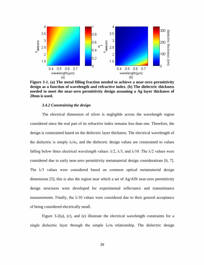
Figure 3-1. (a) The metal filling fraction needed to achieve a near-zero permittivity design as a function of wavelength and refractive index. (b) The dielectric thickness needed to meet the near-zero permittivity design assuming a Ag layer thickness of 20nm is used. ............................................................................................................. 39
Figure 3-2. The left column of plots represents the electrical length of a dielectric as a function of refractive index and wavelength, when reduced according to (a) λ/2, (c) λ/3 and (e) λ/10 design constraints. The right column of plots represent the region in which Figure 2-3 (b) remains valid under the (b) λ/2, (d) λ/3 and (f) λ/10 design constraints, with the scale representing the margin in which the dielectric thickness meets the design constraint. The dotted lines on the right column plots represent dispersion curve for AlSb, AlAs, AlN, Al2O3, SiO2 and MgF2 from top to bottom. 40

7
Page
Figure 3-3. (a) Index of refraction results from ellipsometry measurements for a 22nm Ag layer compared to Palik’s data [36]. The solid lines refer to Palik’s data, and the markers refer to measured values. (b) Index of refraction results from ellipsometry measurements on 83nm of AlN. ................................................................................ 42
Figure 3-4. Experimental (‘o’ marked lines) reflectance (left) and transmittance (right) results compared to transfer matrix method modeling (solid lines) for the single- (p=1), two-, three-, and four-period (p=4) sample. The material thicknesses used were 22nm and 83nm for Ag and AlN respectively. ................................................. 43
Figure 3-5. EMT modeling predictions for a single- to four-period near-zero permittivity design. The material thicknesses used were 22nm and 83nm for Ag and AlN, respectively. ............................................................................................................... 44
Figure 3-6. λ/10 model-to-model comparison for a four period design using 20nm silver layer thickness and the dielectric thicknesses prescribed by EMT analysis. ............. 45
Figure 4-1. Condition number plot for DRR under a 48-measurement collection configured with a λ/5 (a) and λ/3 (b) retarder. The x-axis refers to angular increments applied to the generator retarder, and the y-axis analyzer retarder increments. ................................................................................................................. 53
Figure 4-2. Condition number plot for the retardance cases tested (a) λ/5 (b) λ/4 and (c) λ/3 for the retarder rotation ratios 34:26, 37.5:7.5 and 25:5. ..................................... 57
Figure 4-3. Ideal free-space intensity signal under three different DRR retardance conditions (λ/5, λ/4 and λ/3) when the retarders are rotated under a ratio of (a) 34:26, (b) 37.5:7.5 and (c) 25:5. ........................................................................................... 58
Figure 4-4. Expected error in the free-space Mm extraction for the rotation ratios, θA:θ G = 34:26 (blue), 25:5 (green) and 37.5:7.5 (red) using the three retardance restrictions (a) δ=λ/5, (b) λ/4 and (c) λ/3 and varying the number of intensity measurements (q) when additive random errors were introduced to ideal modeled intensity measurements for the DRR configuration represented. ............................................. 60
Figure 4-5. Comparison of (a) modeled error in the free-space Mm extraction with the (b) experimental error for the instrument configured with ~λ/3 retarders in the DRR for three rotation ratio configurations (θA:θG = 34:26, 25:5 and 37.5:7.5). .................... 62
Figure 5-1. Physical layout of the Mueller matrix scatterometer using the following labeling conventions: TM – turning mirror; BC – beam combiner; Ch – chopper; PH – pinhole; FL – focusing lens; OAP – off-axis parabolic mirror; GP – generator-stage polarizer; GR – generator-stage retarder; AR – analyzer-stage retarder; AP – analyzer-stage polarizer. ............................................................................................ 68

8
Page
Figure 5-2. Nominal retardance for the achromatic waveplate designed for 7.4-10.6µm. Similar retardance behavior is expected for the 4.3-6.5µm achromatic waveplates. 71
Figure 5-3. Mm specular reflectance plot for a novel optical metamaterial sample [33] at 5.0µm when the instrument was operating as a Mm polarimeter. I.e. in specular mode such that the angles represent both incident and reflected angle. .................... 73
Figure 5-4. Mm BRDF of a novel optical metamaterial sample [33] at 5.0 µm and 25o incident angle. The resonant feature of Figure 5-3 is repeated here. The periodic structure is diffraction orders generated by the periodic nature of the sample. ......... 74
Figure 5-5. Mm BRDF of a novel optical metamaterial sample [33] at 5.0 µm and 60o incident angle, illustrating the off-resonant condition. The diffraction orders seen in Figure 5-4 are again found here. ................................................................................ 74
Figure 6-1. (left) P-pol and (right) s-pol reflectance measurements taken of the MMA with increasing incident angle using the IR-VASE ................................................... 79
Figure 6-2. Surface plasmon polariton resonance calculated for the MMA, using the material properties of Au at 5.0µm (ñ = 3.7+ i30.5) [34] and the dielectric (ñ = 2.06 +0.12) [17], while the periodic spacing a= 3.2µm..................................................... 81
Figure 6-3. Normalized specular reflectance Mm plot for the MMA at 5.0µm. .............. 81
Figure 6-4. The trace of MMT for the extracted specular reflectance Mm for the MMA at 5.0µm. ........................................................................................................................ 83
Figure 6-5. Rs (green) and Rp (blue) reflectance behaviors determined from un-normalized Mm data for the MMA at 5.0µm. Markers represent reflectance data from the IR-VASE measurement............................................................................... 85
Figure 6-6. Ratio of the reflectances (top) and phase difference between the p-pol and s-pol reflectances (bottom). .......................................................................................... 87
Figure 6-7. Modeled Fresnel reflectance and phase curves for gold (surface material of MMA) at 0.2µm (a) and (b) (ñ = 1.427 + i1.215) and 5.0µm (c) and (d) (ñ = 3.7 + i30.5). ......................................................................................................................... 89
Figure 6-8. Modeled Fresnel reflectance curves for an anisotropic uniaxial material, where nx = ny = 3.7, κx = κy = 30.5, nz = 3 (a), 0.3 (b), 0.03 (c), and 0.003 (d) κz = 0.01. ........................................................................................................................... 90
Figure 6-9. Predicted Fresnel reflectances using an anisotropic biaxial model (nx = 0.03, κx = 0.05, ny = 3.7, κy = 30.5, nz = 0.45, κz = 0.01). .................................................. 91

9
Page
Figure 6-10. Stokes plots for the MMA when canonical Stokes polarization states (a) horizontal (b) +45˚ and (c) right-hand circular are applied to the extracted Mm, with the respective incident Stokes vector shown below each plot. .................................. 92
Figure 6-11. The ellipticity (χ) and major axis orientation (ψ) of the reflected Stokes vector with linear +45o (left) and right hand circular (right) polarization states incident on the MMA at 5.0µm. ................................................................................ 93
Figure 6-12. Traces of the reflected polarization states on the Poincaré sphere for the MMA when the incident wavelength is 5.0µm and the polarization state is linear +45o (left) and RHC (right)........................................................................................ 94
Figure 7-1. Theoretical MMA design (top) where the available unit cell dimensions are varied to show the expected changes in the resonant response [74]. ......................... 97
Figure 7-2. A wide-band MMA design (left) with its measured absorption (right) [75]. 97
Figure 7-3. A non-multiplexed (a) and multiplexed (b) MMA design with the measured reflectance (c) [76]. .................................................................................................... 98
Figure 7-4. Scanning electron microscope (SEM) image of releasable IR metamaterial flakes (left) and the spectral reflectance (right), with the right axis depicting the measured results for the flakes [77]. .......................................................................... 98
Figure 7-5. SEM image (left) for a photonic crystal made of tungsten, which demonstrated a photonic bandgap over 8-20µm [78]. ............................................... 99
Figure 7-6. SEM image of cubic dielectric array (left) with the unique reflectance and transmittance spectra (right) [79]. .............................................................................. 99
Figure A-1. Comparison of complex refractive index data from Johnson [37] (a) and (c) Palik’s [36] (b) and (d) for the noble metals copper (Cu), gold (Au) and silver (Ag). ................................................................................................................................. 107
Figure A-2. Modeled reflectance and transmittance spectra for a 30nm layer of Ag using the complex refractive index data from Johnson [37] (left) and Palik [36] (right). 108
Figure A-3. Comparison of complex permittivity data from Johnson [37] (a) and (c) and Palik [36] (b) and (d) for the noble metals copper (Cu), gold (Au) and silver (Ag). ................................................................................................................................. 109
Figure A-4. The real part of the complex permittivity from Palik’s data [36], which show the zero crossings. .................................................................................................... 110

10
Page
Figure A-5. EMT to TMM modeling comparison of a four period structure at the design wavelengths of 0.35 and 0.4µm for the refractive indexes n=2, 3 and4. ................. 112
Figure A-6. EMT to TMM modeling comparison of a four period structure at the design wavelengths 0.47 and 0.55µm for the refractive indexes n = 2.0 and n = 4.0, respectively. ............................................................................................................. 112
Figure B-1. The modeled m10 term of the normalized reflectance Mm for a gold mirror. ................................................................................................................................. 114
Figure B-2. The modeled m22, m23, m32, and m33 terms of the normalized reflectance Mm for a gold mirror. ...................................................................................................... 114
Figure B-3. Modeled-to-measured results comparison of the m22, m23, m32, and m33 elements of a Mm reflectance for a gold mirror at 3.39µm and 5.0µm................... 115
Figure B-4. Mm plot for a gold mirror at 3.39µm. ......................................................... 116
Figure B-5. Mm plot for a gold mirror at 5.0µm. ........................................................... 117

11
LIST OF TABLES
Page
Table 2-1. Ideal polarizer measurements for Stokes vector specification ........................ 29
Table 5-1. EC-QCLs selected for the Mm polarimeter-scatterometer .............................. 69
Table 5-2. EC-QCL wavelength stability performance under different bias conditions .. 69
Table 8-1 List of Contributions....................................................................................... 106
Table A-1. λ/10 design values tested for TMM and EMT agreement ............................ 111

12
DESIGN AND CHARACTERIZATION OF OPTICAL METAMATERIALS USING TUNABLE POLARIMETRIC SCATTEROMETRY
I. INTRODUCTION
1.1 Optical Metamaterials and Effective Media
Optical metamaterials are a class of engineered materials, typically made from
metal and dielectrics, designed to interact with optical frequencies at terahertz (THz),
infrared (IR) and visible wavelengths. These materials are designed to obtain their
electromagnetic behavior from a unit structure which is much smaller than the designed
wavelength of interest. By having a subwavelength periodicity, they are distinguished
from photonic bandgap and photonic crystal structures [1, 2]. When the unit cell and
inclusion dimensions of these materials are very small in comparison to the design
wavelength, the optical materials can also be afforded an effective media description [4].
Optical metamaterials’ electromagnetic properties (permittivity - ε and
permeability - µ) can be considered macroscopic and afforded an effective medium
theory (EMT) description by using the inclusion size (δ) and the unit cell period (a) in the
assessment. It has been suggested that these material features should adhere to the
inequality [4]
( , )0.01 0.2.aδλ
< < (1-1)
Meeting these limits has been especially difficult as optical wavelengths are approached.
A review of how well optical metamaterials designed for negative refractive index were
adhering to these limits was shown by Soukoulis [5]. As the visible optical wavelengths
were approached, the best achieved unit cell periodicity was on the order of a/λ = 0.5. It

13
was pointed out that it is difficult to argue that EMT could validly be used with this level
of constraint and that a new design is needed to reduce the design dimensions and
recover the justification of using EMT to describe the macroscopic behavior of these
materials. Thus, the coexistence of an optical metamaterial and an effective medium
description have been difficult to achieve.
1.2 Problem Statements
1.2.1 Validating the Use of Effective Medium Theory
The valid use of EMT in optical metamaterials research is not isolated to negative
refractive index materials; it is a global challenge in optical metamaterials research. This
has been revealed in some of the simplest metamaterial structures, periodic layered
metal-dielectric structures [6, 7, 8], which were used to achieve near-zero permittivity (ε)
material properties at visible wavelengths. The near-zero permittivity property is
achieved by diluting the metal’s permittivity. This is accomplished by pairing the metal
with a positive permittivity material (i.e. a dielectric) in a periodic, layered material
design. The thickness of the dielectric is determined by EMT calculations but will not
properly describe/predict the post-fabrication behavior of these materials unless an
appropriate dimensional constraint is applied to the dielectric thicknesses [8].
1.2.2 Instrument Demand for Infrared Metamaterials Research
A full directional, full polarimetric instrument which can target the narrow-band
features of optical metamaterials is need to adequately experimentally determine the
behavior of optical metamaterials. In particular, the instrument should target infrared (IR)

14
wavelengths because the natural progression of optical metamaterial designs is from IR to
visible wavelengths, and would thereby permit the early identification of problems.
The theoretical predictions of metamaterial properties of interest (ε and µ) will
often depend on incident angle and the polarization state of the incident radiation [9]. The
optical phenomenon of these materials, often Bragg or plasmonic resonances, are
frequently narrow-band in nature [10, 11]. Typical methods of analyzing these materials
have been Fourier-transform spectrometery (FTS) specular transmittance [12-15],
reflectance [16-18], emission [19-25] and IR specular spectraphotometric transmittance
and reflectance [26, 27] and Variable-Angle Spectrometric Ellipsometry (VASE) [10].
However, the ability to perform optical characterization of fabricated samples which are
complete from a spectral, polarization and directional point-of-view has not been
available to IR metamaterial researchers.
1.3 Research Objectives
A series of research objectives was assembled to address the use of EMT in the
simplest structures of metamaterial research and address the absence of an instrument
capable of meeting the full-directional and full-polarization characterization demands of
IR metamaterials.
• Model, design, fabricate and test an optical near-zero permittivity structure and identify the appropriate design constraints to apply for EMT usage in the design and post-fabrication analysis steps
• Develop an optimal dual rotating retarder (DRR) polarimeter which is compatible with mid-wave infrared (MWIR, 4.37-6.54µm) and long-wave infrared (LWIR, 7.41-9.71µm) wavelengths

15
• Develop the first tunable IR Mm polarimeter-scatterometer for the characterization of IR optical metamaterials
• Measure an IR metamaterial with the tunable IR Mueller matrix (Mm) polarimeter, determine the appropriate model needed to replicate the experimental results, and perform polarimetric analysis using canonical polarization states to describe the measured results
1.4 Research Objective Accomplishment
The research objectives in this research were primarily accomplished in a model,
design, and then experimentally verify approach.
1.4.1 EMT use in periodic metal-dielectric near-zero permittivity designs
Models were built and used to deduce the experimental behaviors seen in near-
zero permittivity research conducted at visible frequencies [6, 7]. The findings were that
a transfer matrix method (TMM) model predicted the behavior and an EMT-derived
model, although leveraged in the design steps, did not accurately predict the experimental
results. Novel research steps were taken in this document to design and develop a series
of near-zero permittivity structures to make clear the model that produces the
experimental findings is the TMM model. The design constraints necessary for reaching
agreement between the TMM and EMT models were then found and used to identify the
design region where EMT could validly be used in the design and experimental analysis
steps [8].
1.4.2 Development of an IR Mm Polarimeter Scatterometer
The development of a tunable IR Mm polarimeter-scatterometer is a multi-faceted
problem. The starting point was a Schmitt Measurement Systems (SMS) Complete Angle
Scatter Instrument (CASI®) and optics capable of implementing a DRR polarimeter at
3.39µm and 10.6µm. This instrument needed beam train modifications to introduce a

16
series of tunable external-cavity quantum cascade lasers (EC-QCLs) and a set of
experimental methodologies that could be used to leverage the use of the 3.39µm and
10.6µm optical components. When it was determined that a DRR design, compatible with
the EC-QCLs, could not be achieved with the on-hand optics [28], the findings were
applied to a new research objective directed at determining the best possible design. The
optimal design was determined using a novel modeling approach [29, 30] and, when
implemented, it led to the first third-wavelength DRR design to be used in a Mm
scatterometer [31].
1.4.3 Measuring and Modeling an IR Metamaterial
The abilities of the tunable IR Mm polarimeter-scatterometer were confirmed
when the first Mm-polarimeter measurements were collected on an IR metamaterial
absorber (MMA) [33]. The MMA was found to have an incident angle depend resonance,
which was captured with Mm polarimetry measurements conducted at 5.0µm. Modeling
steps were then used to distill the polarized reflectance and reflectance phase information
which was responsible for this behavior. Additionally, example behaviors of this material
under the influence of incident canonical polarization states were analyzed and explained
from using the extracted Mm results.
1.5 Organization
This document is organized according to the accomplishment of each of the
research objectives, which are preceded with background material and followed with
conclusions. Chapter 2 provides background information needed to introduce the material
coved in Chapters 3-6. Chapter 3 covers the modeling, design, fabrication and

17
experimental analysis of near-zero permittivity structures. Chapter 4 covers the
development of the DRR needed for the wavelength tunable, polarimetric IR instrument.
Chapter 5 covers the development of the tunable IR Mm polarimeter-scatterometer and
the novel measurements validating its use. Chapter 6 covers the unique measurements,
modeling and polarimetric analysis of an IR metamaterial. Chapter 7 covers future work
following the successful development of the tunable IR Mm polarimeter-scatterometer,
where several recently developed IR samples from literature are identified. Chapter 8
covers the overall conclusions to the research contained in this document.

18
II. BACKGROUND
The goal of this chapter is to provide the background material for the problems
confronted in this research. Each section is aligned with a research objective and a
chapter of this document.
2.1 Near-Zero Permittivity Structures
The contents of this section provide the background information needed to
introduce the research covered in Chapter 3 “Modeling Design and Experimental
Analysis of Near-Zero Permittivity Structures at Optical Wavelengths.”
Tailoring the permittivity (ε) of materials is a broad metamaterial topic. The field
of research was restricted to stratified, composite materials directed at achieving a near-
zero permittivity. This research recently became relevant when the near-zero permittivity
property was theoretically predicted to be useful for enhancing the transmission of
extraordinary transmission devices [32]. Two attempts at developing these material
properties at optical frequencies in the visible have been conducted [6, 7] by using metal-
dielectric layered media. Effective medium theory (EMT) and mixing fractions were used
to arrive at the dielectric material design thicknesses, while the metal used (silver - Ag)
was restricted to thicknesses on the order of 20-30nm (where a continuous layer that is
still transmissive can be achieved). Claims at achieving the near-zero permittivity were
made despite clear evidence that the material layers used were too thick, leading to
oscillatory behavior in the measured reflectance and transmittance spectra. There were no
attempts to restrict the dielectric thickness to levels necessary to leverage EMT in the
design and post-fabrication analysis steps.

19
The novel approach taken in my research was to first design a near-zero
permittivity structure consistent with literature through the use of EMT and mixing
fractions, then show the appropriate theory for modeling and post fabrication predictions
should be the transfer matrix method (TMM) [8, 35] (unless appropriate design
constraints are imposed, i.e. dielectric thicknesses). The EMT design would then be
expanded to look at a range of refractive index scaled dielectric thicknesses (i.e. electrical
length) where the EMT modeling results were found to be in agreement with the TMM
results – to identify the practical design constraints needed to achieve an optical near-zero
permittivity design. With these design constraints imposed, the reflectance and
transmittance spectra could be expected to be void of oscillatory behavior above the
design wavelength and have near-zero permittivity properties at the design wavelength.
In order to carry this research out, the development of four periodic metal-
dielectric (Ag/AlN, 20nm/80nm) layered structures for a 630nm near-zero permittivity
crossing were specified. The fabrication was carried by Naval Air Warfare Center
Weapons Division in China Lake, CA where the staff has decades of optical fabrication
experience. A depiction of the samples is shown in Figure 2-1. The TMM and EMT
modeling are covered in Chapter 2, along with the near-zero permittivity design
methodology, which shows how to arrive at a dielectric thickness that will deliver a zero
permittivity crossing at a desired wavelength.
The origin of the oscillatory features became clear when the TMM and EMT
models were built to replicate the experimental data in the near-zero permittivity designs
found in [6] and [7]. The TMM- and EMT-derived results are shown in Figure 2-2 and
provided the impetus for this research – the TMM and EMT results were clearly not in

20
Figure 2-1. The set of four Ag/AlN layered near-zero permittivity design structures on transparent substrate, where the grey layers refer to Ag and the blue layers refer to AlN.
agreement. Figure 2-3 is used to show the zero permittivity crossing for each of the
designs [6, 7], which comes from using the EMT (essentially volumetrically averaging
the materials) in the design steps. It should be noted here that Palik’s bulk material data
for Ag [36] was used to generate the plots found in Figures 2-2 and 2-3. It was found to
achieve the best agreement between the model and experimental results. Appendix A
spends some time elucidating the details on why Palik’s [36] rather than Johnson’s bulk
data [37] provides more accurate results at the optical wavelengths in these design
regions.
Figure 2-2. Reflectance (red) and transmittance (blue) modeled results for [6] using TMM (a) and EMT (c) and for [7] using TMM (b) and EMT (d).
substrate substrate substrate substrate

21
Figure 2-3. Permittivity results using mixing fractions to achiev a zero crossing for [6] (left) and [7] (right). The zero crossing of the permittivity for [6] was 580nm and 520nm for [7].
On a final note here, a brief discussion is needed to understand what kind of result
should be predicted from a near-zero permittivity design. The short answer is it should
behave as a perfect reflector because it emulates an infinite impedance mismatch with
free-space. This reflective condition is readily accessible by first examining the
relationship between the permittivity (ε) and refractive index (n)
,n εµ= (2-1)
where µ refers to the permeability of the material. At optical frequencies, the
permeability of materials is generally unity, leading to a simplification of the relationship
and shows a near-zero permittivity leads to a near-zero refractive index. When a near-
zero refractive index is inserted into the Fresnel reflectance equation (at normal
incidence), 2
0
0
ENZ
ENZ
n nRn n
−= +
the strong reflective character is predicted since the
reflectance (R) evaluates to unity. High reflectivity is predicted in the near-zero
permittivity plots of Figure 2-2, just after the intersection of the transmittance and

22
reflectance curves, and will similarly be manifested in the TMM modeling results when
the appropriate design dimensions are applied [8].
2.2 Dual Rotating Retarder Optimization
The contents of this section provide the background information needed to
introduce the research covered in Chapter 4 “Optimizing a Dual Rotating Retarder for a
Tunable Infrared Mueller-Matrix Polarimeter-Scatterometer.”
A dual rotating retarder (DRR) is considered a complete polarimeter, that is, it
leads to the full polarimetric specification of a sample under test through determining the
Mueller matrix (Mm) of that sample [38]. A diagram of a DRR is shown in Figure 2-4,
which shows two fixed linear polarizers that are co-aligned and two linear rotating
retarders, one in front of and one behind the sample under analysis. The linear polarizer
Figure 2-4. Illustration of a dual rotating retarder (DRR) in a transmission measurement configuration. The retardances specified (δG = δA = λ/5, λ/4 and λ/3) represent values examined during the optimization process.
Rotating Linear Retarder δΑ= λ/5,λ/4,λ/3
Rotating Linear Retarder δG = λ/5,λ/4,λ/3
Fixed Linear
Polarizer
Fixed Linear
Polarizer
Sample M Detector
θG θA
Polarization State Analyzer
Polarization State Generator

23
and retarder in front of the sample make up the polarization state generator (PSG) stage,
and the linear polarizer and retarder behind the sample make up the polarization state
analyzer (PSA) stage. As shown, the DRR is in a transmission configuration, but the PSA
can be rotated about the sample to operate in reflection too. Here, it can be used to
observe specular reflection from the sample (acting like a Mm polarimeter) or off-
specular angles to observe the polarimetric content of scatter (acting like a Mm
scatterometer).
2.2.1 Discussion of the optimization problem
The simplest equation representing the measurement of a sample with a DRR
polarimeter is
,I WM= (2-2)
where I represents a matrix of the intensity measurements collected for incremental
retarder rotation positions, W is a matrix representing the optical components of the DRR,
and M represents the Mm of the sample under test. There are two pieces to the
optimization problem. First, all the optical components are summed up in W. If these
components are not well-known, or if there are misalignments among the optical
components, systematic errors will be introduced to the intensity signal. These systematic
errors will subsequently be introduced to the Mm of the sample (M) when a W-matrix
that does not accurately represent the DRR is used in the inversion process of Eqn. (2-2)
to find M. Second, if W is well-known but ill-conditioned (too little retardance, too few
measurements, or a poorly selected rotation ratio), then high levels of error can be
introduced to the extracted Mm [39]. It is a calibration technique that mitigates the first
problem [39, 40]. It is the body of research, contained in Chapter 4, that uniquely

24
addresses the second problem and led to the first third-wavelength achromatic DRR to be
used in a Mm scatterometer [29, 30].
2.2.2 The unique optimization solution – random error analysis
Three retardance values are shown in Figure 2-5, fifth, fourth and third-
wavelength (λ/5, λ/4 and λ/3, respectively) and represent: the retardance available during
the initial design stages of the tunable Mm scatterometer development; the common DRR
retardance configuration for the Fourier method [41]; and the optimal retardance
configuration [42, 43]. High levels of error from measurements collected with the DRR
using λ/5 retarders (which were on-hand), despite employing optimization methods from
[43]. It was by mathematically applying a constant level of random error to free-space
intensity measurements (I in Eqn. (2-2), with M as the identity matrix), and varying the
retardance and rotation ratios (each contained in W of Eqn. (2-2)), that the origin of the
error was determined. It was insufficient retardance [28]. This same process was then
used to determine the optimal DRR configuration – a Fourier retarder rotation ratio and
λ/3 retarders were found to be optimal [29, 30].
2.3 Tunable Infrared Mueller-matrix Polarimeter-Scatterometer
The contents of this section provide the background information needed to
introduce the research covered in Chapter 5 “Development of a Tunable Infrared
Mueller-Matrix Polarimeter-Scatterometer.” The previous section and the contents of
Chapter 4 dealt with DRR operating theories, calibration methods and the modeling used
to identify the optimal DRR configuration for the tunable IR Mm polarimeter-
scatterometer. This section examines the starting point of the instrument, practical

25
implementation of the DRR configuration to ensure compatibility with the set of tunable
external-cavity quantum cascade lasers (EC-QCLs).
2.3.1 Complete Angle Scatter Instrument
The starting point for the tunable infrared (IR) Mueller-matrix (Mm) polarimeter-
scatterometer development was a Schmitt Measurement Systems (SMS) Complete Angle
Scatter Instrument (CASI®). In its original state, the CASI® was a scalar scatterometer,
that is, it measured the scalar form of the bi-directional scatter distribution function
(BSDF) of a sample by transmission or reflection measurements. The BSDF has units of
steradian-1 defined according to [44]
1( , ) ,( , )
s sBSDF
i i
Lf srE
θ φθ φ
−= (2-3)
where L is the scattered radiance (in reflection or transmission), θs is the observed scatter
angle, φs is the observed scatter azimuth angle, E is the irradiance, θi is the incident angle,
and φi is the incident azimuth. For in-plane measurements, φs - φi. = 180o. The
polarimetric form of the instrument is realized with the introduction of the DRR. In the
polarimetric form, the BSDF becomes a Mm according to [45]
0 00 01 02 03 0
1 10 11 12 13 1
2 20 21 22 23 2
3 30 31 32 33 3
( , ) ( , ) ,s s i i
out in
S f f f f SS f f f f S
L ES f f f f SS f f f f S
θ φ θ φ
=
(2-4)
where Sin is a Stokes vector (discussed in Section 2.4) representing the polarization state
which is incident on the sample and Sout represents the polarization state after
encountering the sample. It is in this form that the mechanics of operating the instrument

26
as a scatterometer versus a polarimeter can be seen. When θi is held constant but θs is
allowed to vary during measurements, the instrument is operated as a scatterometer.
When θi and θs are equal, and φs - φi. = 180o, the instrument is operated as a polarimeter.
The later of these configurations is generally exercised for very specular samples, while
the former is exercised with a sample having diffuse or diffractive qualities. The Mm
polarimeter functionality was introduced to the instrument during this research using
external programming features.
2.3.2 Practical design considerations
The CASI® contained four different laser sources: 633nm, 533nm, 3.39µm and
10.6µm. Optics were available to implement a DRR at each of the discrete wavelengths.
Two primary tasks for developing the tunable IR Mm polarimeter-scatterometer were
identified at the beginning of this research: modify the existing optical beam train to
introduce the six tunable EC-QCLs to the CASI®; and determine a way to use the
existing sets of IR quarter-wave retarders for a DRR which is compatible with the six
EC-QCLs. The beam train modifications are covered in Chapter 5. The findings from the
attempts to implement the DRR with the existing set of quarter-wave retarders are
covered here.
The difficulty with implementing a DRR to be compatible with the EC-QCLs
using existing 3.39µm and 10.6µm quarter-wave retarders can be summarized with: the
hind-sight knowledge presented in Section 2.2 (retardances less than 90o should generally
be avoided); the modeled retardance for the retarders in Figure 2-5; and the spectral
transmission curves for the retarders in Figure 2-6. First, Figure 2-5 shows the 3.39µm

27
retarders should not be considered due to a lack of retardance. This figure does suggest
the 10.6 µm retarders may be viable down to 7.0µm (where the modeled retardance
reaches 135o), but the EC-QCL source covering this wavelength range broke and was
Figure 2-5. Expected retardance curves for the 3.39µm quarter-wave retarder (left) and 10.6 quarter-wave retarder (right).
Figure 2-6. Measured transmission curves for the 3.39µm quarter-wave retarder (red) and 10.6 µm quarter-wave retarder (blue). The approximate spectral range of each EC-QCL (each represented by an individual color) is overlayed. unavailable for over 6 months. Figure 2-6 shows why the 3.39µm and 10.6µm quarter-
wave retarders should generally be avoided. The anti-reflective coatings did not span the

28
wavelengths covered by the EC-QCLs (4.35-9.71µm). These findings led to the research
work covered in the previous section and illustrate non-trivial steps in the development of
this instrument.
2.4 Mm Measurements and Modeling of Novel Metamaterial Absorber
The contents of this section are used to briefly introduce the material to be
covered in Chapter 6 “Evaluation of a Novel Optical Metamaterial Absorber.”
A metamaterial absorber (MMA) [33] was the first sample analyzed with the Mm
polarimeter-scatterometer. An IR variable angle spectrometric ellipsometer (IR-VASE)
was used to examine the p-polarized and s-polarized reflectances of the sample for
resonant features of interest in the tunable range of the Mm polarimeter-scatterometer. A
narrow-band feature with incident angle dependence was found at 5.0µm, which was
subsequently analyzed with the Mm polarimeter-scatterometer. A Mm reflectance model
was used to interpret the findings [38], while Fresnel reflectance models (isotropic,
uniaxial anisotropy and biaxial anisotropy) were evaluated for agreement with the
findings. The Mm reflectance model had been successfully used to corroborate Mm
polarimeter measurements conducted on a gold mirror following the instrument
development and was leveraged in the Mm analysis of the MMA in Chapter 6.
Most importantly, the measured Mm for the MMA was found physically
realizable. This permitted follow-on polarimetric analysis of the MMA using the
measured Mm results. Example behavior of the MMA was modeled under the
assumption canonical polarization states incident on the material. These were analyzed
via Stokes and Poincaré sphere representations. Background information on Stokes

29
vectors and Poincaré sphere are provided here, while the Mm reflectance model is
covered in Chapter 6.
2.4.1 The Stokes Vector and its Poincaré Sphere Representation
A first principles development of the Stokes vector can be found in [46].
However, it is the phenomenological definition of the Stokes vector [38] and its
specification in terms of the angles χ and ψ in the Poincaré sphere [46] that led to the
greatest insight into interpreting the behaviors of an extracted Mm. So, it is the
phenomenological representation of the Stokes vector and its Poincaré sphere
representation that is presented here.
The Stokes vector is a four element vector which fully defines the polarization
state of an optical signal. It can be constructed from a series of six intensity
measurements with ideal polarization elements [38]. The ideal polarizer measurements
are listed in Table 2-1.
Table 2-1. Ideal polarizer measurements for Stokes vector specification
IH Intensity measurement from a linear polarizer oriented at 0o
IV Intensity measurement from a linear polarizer oriented at 90o
I45 Intensity measurement from a linear polarizer oriented at 45o
I135 Intensity measurement from a linear polarizer oriented at 135o
IR Intensity measurement from a right hand circular polarizer
IL Intensity measurement from a left hand circular polarizer
These measurements can be used to specify the Stokes vector by
0
1
2 45 135
3
.S
H V
H V
R L
S I IS I IS I IS I I
+ − = = −
−
(2-5)

30
The Stokes vector can also be specified in terms of the angles χ (ellipticity) and ψ
(orientation) in the Poincaré sphere to visually depict the polarization state [46]. The
Stokes vector can also be represented in terms of χ and ψ.
0
1
2
3
1cos(2 )cos(2 )cos(2 )sin(2 )
sin(2 )
SSSS
χ ψχ ψ
χ
= =
S (2-6)
If the Stokes vector is known, the values χ and ψ for a Poincaré sphere illustration of the
Stokes polarization state can be found. Figure 2-7 illustrates the Poincaré sphere. The
linear polarization states reside on the equator. The right-hand circular state resides at the
north pole, and the left hand circular state resides at the south pole. The right hand
elliptical states reside between the equator and the north pole, and the left hand elliptical
states reside between the equator and the south pole.
Figure 2-7. The Poincaré sphere with the canonical polarization states depicted (left) and a right hand elliptical polarization state depicted (right). The ellipticity (χ) is measured from the S1S2-plane, where the linear polarization states exist, and the orientation (ψ) is measured from the S1-axis. RCP refers to right-hand circular polarization.
2χ
2Ψ

31
2.5 Conclusion
This chapter was used to introduce some of the details needed to transition into
the research topics that follow in a chapter-by-chapter basis. This document was
organized in a scholarly format, where Chapters 3-6 individually represent research
which has either been published, submitted for publication or is in the preparatory steps
of submitting for publication. The status of publications is cited in the introductory
paragraph of each chapter.

32
III. MODELING, DESIGN AND EXPERIMENTAL ANALYSIS OF NEAR-ZERO PERMITTIVITY STRUCTURES AT OPTICAL WAVELENGTHS
This chapter covers the research work directed at modeling, design, and
experimental analysis of a set of near-zero permittivity structures. The content of this
chapter has been accepted for publication in Optics Express [8]. The primary research
contribution was determining the appropriate design constraints to apply to composite,
stratified media for agreement between the transfer matrix method (TMM) and effective
medium theory (EMT) modeling, thereby permitting EMT to be used in design and post-
fabrication analysis, and equivalently, identifying the limits of its use.
3.1 Executive Summary of Research
The design and analysis of near-zero permittivity structures composed of periodic
metal-dielectric thin films are examined from transfer matrix method (TMM) and
effective medium theory (EMT) modeling approaches. Dimensional constraints of λ/2,
λ/3, and λ/10 are enforced for designs using silver paired with a dielectric having a
refractive index in the range of 1.2 to 4.0. The wavelengths considered span 0.35 to
0.75μm. To ground the modeling results, a set of four ~λ/3 silver/aluminum nitride
(Ag/AlN) near-zero permittivity structures was designed, fabricated and analyzed. Their
reflectance and transmittance were found to be in excellent agreement with the TMM
analysis, but in poor agreement with the EMT analysis. A λ/10 design substantially
narrows the available design region (0.35 to 0.55μm) but is suggested due to the
agreement found between TMM and EMT across these wavelengths.

33
3.2 Introduction
The interest in ultralow refractive index materials (ULIM’s), and similarly,
epsilon-near-zero (ENZ) materials at optical frequencies is growing. ULIM’s with near
unity index have been achieved by introducing porosity while maintaining specularity
[47-51]. These ULIM’s are useful for achieving anti-reflection due to their low-level of
impedance mismatch with free space. They are also useful for optical confinement of
solid core and air core [52] optical waveguides, where the former ULIM maintains an
effective index near unity and the latter index approaches zero through a near-zero
permittivity design.
Metals have a naturally occurring near-zero permittivity, which appears at their
plasma frequency then becomes increasingly negative as the frequency is reduced (i.e. as
wavelength is increased) [36]. The material response at the zero crossing in the
permittivity marks where the material transitions from transmissive to highly reflective,
due to the increasing imaginary component of the refractive index. Zero permittivity
materials can also be engineered. This first took place for microwave frequency
applications decades ago through fabricating arrays of wires which resulted in a zero-
permittivity crossing [53, 54]. With the introduction of metamaterials and enhanced
computational capabilities, this zero-permittivity design was later analytically extended to
infrared wavelengths [55, 56]. A novel method for achieving ENZ properties has recently
been achieved through manipulating the geometry of a waveguide channel rather than
strictly engineering material properties [57]. Most recently, an infrared ENZ design was
developed through heavily doping InAsSb to modify its dispersion behavior [34].

34
In this chapter, the use of mixing fractions in a layered metal-dielectric structure
with a zero-permittivity design goal is examined. The modeling theory for thin films and
its extension to effective medium theory (EMT) through a long-wavelength
approximation are first examined. Then, the design methodology of a near-zero
permittivity thin-film structure using an effective medium approach is examined. The
design is completed as a function of wavelength and refractive index, and leads to a plot
of dielectric thickness designs which deliver a zero-permittivity crossing. These dielectric
thicknesses are then constrained for model comparison of λ/2, λ/3, and λ/10 designs.
Experimental results for a ~λ/3 Ag/AlN design are then used to ground the dimensionally
constrained modeling.
Similar layered media approaches have been undertaken to design zero-
permittivity materials at optical wavelengths [6, 7]. The analysis completed in this
chapter extends the modeling approach to find where the transfer matrix method (TMM)
and EMT agree to illustrate a valid design region. A λ/3 design corroborates the TMM
modeling methodology, invalidates the use of EMT for this dimension constraint, and
illustrates the need to reduce dimensionality below the λ/2 design constraint suggested
among wired arrays in early metamaterials design work [55, 56]
3.3 Modeling
3.3.1 Transfer Matrix Method
The conventional method for modeling a dielectric stack is to use a TMM, where
each of the constituent layers is accounted for in a two-dimensional matrix [58]. The
same approach can be used for metal-dielectric stacks, with the obvious difference being

35
the use of complex material properties to account for losses present in the metal layers
[6]. For this modeling, only normal incidence is considered, although off-normal
incidence and its corresponding polarization considerations can be accounted for in this
modeling approach [58]. A single material layer is
0 0
0 0
cos( ) sin( )
sin( ) cos( )
j j j jjj
j j j j j
ik n z k n znM
in k n z k n z
− = −
(3-1)
where k0 is the free space propagation constant, ñj is the complex refractive index of the
jth layer, and zj is the thickness of that layer.
To account for a stack of materials, an iterated product of the material layers is
performed starting with the top layer of the material and ending with the layer just above
the substrate. The product is a characteristic matrix representing the stack of thin films
(Mstack).
1
.N
stack jj
M M=
= ∏ (3-2)
The characteristic matrix is then used to determine the amplitude reflection and
transmission coefficients, which are defined in terms of the four elements of Mstack
according to
11 12 0 21 22
11 12 0 21 22
( ) ( )( ) ( )
sub sub
sub sub
m m n n m m nrm m n n m m n
+ − +=
+ + + (3-3)
and
0
11 12 0 21 22
2 .( ) ( )sub sub
ntm m n n m m n
=+ + +
(3-4)

36
The calculation of the reflectance follows the traditional form for calculating the
reflectance from the amplitude reflection coefficients, while the transmittance must be
scaled to account for the substrate material’s refractive index (nsub).
2R r= (3-5)
2
0
subnT tn
= (3-6)
3.3.2 Effective Medium Theory
EMT is capable of leveraging the same 2-D matrix approach with the notable
exception of the iterated product. In this case, the material dimensions of a single period
are assumed electrically small, which allows for the solution of an effective permittivity
and the use of a single 2-D matrix to represent the metal-dielectric stack as a
homogeneous layer (as in Eqn. (3-1)) with the index and permittivity terms replaced with
effective values, and the material thickness replaced with the thickness of the stack (zstack),
as in Eqn. (3-7). The reflectance and transmittance are similarly found through the use of
Eqn. 3-3 through 3-6.
0 0
,
0 0
cos( ) sin( )
sin( ) cos( )
eff stack eff stackeffeff stack
eff eff stack eff stack
ik n z k n znM
in k n z k n z
− = −
(3-7)
3.4 Design
3.4.1Designing for near-zero effective permittivity
The design of a near-zero effective permittivity for a layered metal-dielectric
structure are described here, and the metal filling fraction behavior of silver as a function
of wavelength and dielectric refractive index is examined. In the long-wavelength limit,

37
the effective permittivity of a thin-film structure can be represented as a weighted
average [1]. This functionally allows the permittivity to be tailored within the bounds of
the constituent materials’ permittivities. To calculate the effective permittivity of the
material under design, the parallel component of the permittivity is used, which is
represented in Eqn. (3-8). Here, fm and fd represent the metal and dielectric filling
fractions, respectively (such that fm + fd = 1), and εm and εd are the permittivities of the
metal and dielectric, respectively.
,e par m m d df fε ε ε= + (3-8)
A near-zero permittivity is designed by pairing a metal and dielectric in a
wavelength region below the plasma frequency of the metal. In this region, the
permittivity of the metal becomes increasingly negative and its contribution can be
cancelled through the introduction of a dielectric which inherently possesses a positive
permittivity. When the proper mixing fractions are applied, a near-zero average
permittivity is achieved.
When solving for near-zero permittivity, it is in the designer’s best interest to
solve Eqn. (3-8) for the metal filling fraction because the layer thickness is known and is
generally set to a minimum value (where a continuous film can be practically attained
and still remains transmissive). With the metal layer thickness known and its filling
fraction known, finding the dielectric layer thickness then becomes a straight forward
process. To first solve for the metal filling fraction, the effective permittivity of Eqn. (3-
8) is set to zero, fm + fd = 1 is used to eliminate the dielectric filling fraction, and algebraic
manipulation leads to the functional relationship found in Eqn. (3-9) in terms of the
constituent material permittivities. When the dispersion properties and a range of

38
dielectric permittivities are considered in the design, the functional form for the metal
filling fraction becomes dependent on wavelength and refractive index (a value with
physically intuitive meaning).
1
( )( , ) 1( , )m
md
f nn
ε λλε λ
−
= −
(3-9)
The behavior of the metal filling fraction fm(λ,nd) is plotted in Fig. 3-1(a), where
silver was used as the metal and the range of dielectric refractive indexes spanned 1.2 to
4.0. The wavelength range of 0.35 to 0.75μm was selected to span visible frequencies and
approach the plasma frequency of silver. Using a minimum silver thickness of 20nm, the
dielectric thicknesses were solved for and are plotted in Figure 3-1(b).
Figure 3-1(a) shows that fm increases at short wavelengths and large refractive
indexes. This is due to silver’s low negative permittivity, which is easily offset by a small
amount of the large-positive-permittivity dielectric. At longer wavelengths and lower
refractive indexes, fm diminishes due to the increasing negative silver permittivity, as it
takes a great deal of low refractive index material to offset the silver.
The dielectric thickness plot corroborates the previous explanations for the metal
filling fraction. At short wavelengths and large refractive indexes, only a few nanometers
dielectric are required. At long wavelengths and low refractive indexes, several hundred
nanometers of dielectric are required. The range of dielectric thicknesses spans 5nm to
333nm, and thereby requires constraints to be imposed to avoid encountering unwanted
resonant features in transmittance and reflectance spectra. Under the appropriate
constraints, the design region where thin-film analysis and EMT results agree will be
shown.
39
Figure 3-1. (a) The metal filling fraction needed to achieve a near-zero permittivity design as a function of wavelength and refractive index. (b) The dielectric thickness needed to meet the near-zero permittivity design assuming a Ag layer thickness of 20nm is used.
3.4.2 Constraining the design
The electrical dimension of silver is negligible across the wavelength region
considered since the real part of its refractive index remains less than one. Therefore, the
design is constrained based on the dielectric layer thickness. The electrical wavelength of
the dielectric is simply λ0/nd, and the dielectric design values are constrained to values
falling below three electrical wavelength values: λ/2, λ/3, and λ/10. The λ/2 values were
considered due to early near-zero permittivity metamaterial design considerations [6, 7].
The λ/3 values were considered based on common optical metamaterial design
dimensions [5]; this is also the region near which a set of Ag/AlN near-zero permittivity
design structures were developed for experimental reflectance and transmittance
measurements. Finally, the λ/10 values were considered due to their general acceptance
of being considered electrically small.
Figure 3-2(a), (c), and (e) illustrate the electrical wavelength constraints for a
single dielectric layer through the simple λ0/nd relationship. The dielectric design

40
thicknesses found in Figure 3-1(b) are then subtracted from the constrained values
contained in Figure 3-2(a), (c), and (e). This produces regions of positive and negative
values. The negative values refer to dielectric design thicknesses exceeding the
constraint, while the positive values meet the imposed constraints (by a margin of
thickness). Figure 3-2(b), (d), and (f) show these regions, with the scale reflecting the
Figure 3-2. The left column of plots represents the electrical length of a dielectric as a function of refractive index and wavelength, when reduced according to (a) λ/2, (c) λ/3 and (e) λ/10 design constraints. The right column of plots represent the region in which Figure 2-3 (b) remains valid under the (b) λ/2, (d) λ/3 and (f) λ/10 design constraints, with the scale representing the margin in which the dielectric thickness meets the design constraint. The dotted lines on the right column plots represent dispersion curve for AlSb, AlAs, AlN, Al2O3, SiO2 and MgF2 from top to bottom.

41
margin of thickness by which the dielectric meets the constraints - only a few nanometers
in the case of the λ/10 design. The dotted lines refer to dispersion curves for common
dielectrics; from top-to-bottom, they are AlSb, AlAs, AlN, Al2O3, SiO2, and MgF2. The
next step in the analysis process is examining an actual design to determine the model-to-
experiment agreement and verify the appropriate design constraint based on those results.
3.5 Experimental Results
3.5.1 Layered Material Design
A set of four ENZ structures was designed under a ~λ/3 design constraint, which
span one to four metal-dielectric periods. By developing this particular set of samples, the
influence additional layers have on the ENZ design could be assessed; it also permitted a
robust model-to-experiment verification. The materials selected for the design were silver
and aluminum nitride (nd = 2). Silver was selected for its low loss properties at visible
wavelengths and aluminum nitride was selected to eliminate oxidizing the silver layers
during the deposition process. The design thickness of the silver layers was set at 20nm
and the design wavelength at 630nm, which is far from silver’s plasmonic resonance yet
still in its low-loss wavelength regime [36]. The aluminum nitride layer thickness was
determined to be 80nm, through analysis supported by Eqn. (3-8) and (3-9).
The silver/aluminum-nitride layers were deposited on an Infrasil fused silica
substrate, which provided excellent material qualification results for the silver and
aluminum nitride. Ellipsometry results for index of refraction (nm) and loss index (k) for
the silver deposition show great agreement with Palik’s data [36] in Figure 3-3. The
aluminum nitride was found to have a stable refractive index around 2.0 and lossless

42
across the wavelengths of interest, and is also shown in Figure 3-3. The deposited
thicknesses of the final designs were found to be 22nm and 83nm for silver and
aluminum nitride, respectively.
Figure 3-3. (a) Index of refraction results from ellipsometry measurements for a 22nm Ag layer compared to Palik’s data [36]. The solid lines refer to Palik’s data, and the markers refer to measured values. (b) Index of refraction results from ellipsometry measurements on 83nm of AlN.
3.5.2 Transfer Matrix Method
After finding the material thicknesses through ellipsometry, reflectance and
transmittance measurements were collected under near-normal incidence conditions using
a Perkin Elmer Lambda 950 spectrophotometer and a 150mm integrating sphere
accessory. The ellipsometry-retrieved thicknesses were used in the thin-film analysis
modeling described in Section 3.1 for comparison with the measured reflectance and
transmittance experimental results. The comparisons are shown in Figure 3-4 with the
number of periods increasing from one (p=1) to four (p=4) in the plots from top to
bottom. Excellent agreement exists between the thin-film analysis modeling and the
measured reflectance and transmittance. However, these results are not consistent with
expectations for an electrically small, near-zero permittivity design. The wavelength of
the incident light is still on the order of the dielectric thickness and the phase information

43
from individual material layers is definitely required to attain accurate experimental
predictions.
Figure 3-4. Experimental (‘o’ marked lines) reflectance (left) and transmittance (right) results compared to transfer matrix method modeling (solid lines) for the single- (p=1), two-, three-, and four-period (p=4) sample. The material thicknesses used were 22nm and 83nm for Ag and AlN respectively.
3.5.3 Effective Medium Theory
The experimental results compared to the effective-medium predictive results are
not shown, but there is clearly not agreement between the two. Figure 3-5 shows the
predicted reflectance and transmittance results for all four periodic structures under
effective medium modeling. The transition from high transmittance to high reflectance is
predicted to occur in the 630nm regime. Furthermore, as the number of periods is
increased, the transmittance continues to diminish, which is expected due to the

44
increasing metal contribution. Based on these modeling results, further dimensional
constraints are necessary to yield agreement between the EMT modeling and thin-film
modeling.
Figure 3-5. EMT modeling predictions for a single- to four-period near-zero permittivity design. The material thicknesses used were 22nm and 83nm for Ag and AlN, respectively.
3.5.4 Model-to-Model Agreement
The predictive power of the thin-film analysis technique is apparent from the
results shown in Section 3.5.2 and a design constraint in excess of λ/3 is needed to
achieve agreement between the TMM and EMT modeling. For this reason, comparative
analysis between the two models was performed under a λ/10 constraint. It was here that
the best model-to-model agreement was observed. The perimeter of the dielectric
thicknesses plotted for the λ/10 design in Figure 3-2 was used as a means of verification,
along with the values corresponding to a 0.4μm design wavelength. These results are
illustrated in Figure 3-6. While good agreement between the models exists for the 0.4μm
wavelength designs and along the left hand side of the perimeter (i.e. for a wavelength of
0.35µm, with results found in Appendix A), only a reasonable level of agreement
between the models exists along the diagonal edge of the perimeter, with agreement
decreasing as refractive index increases. This is not a surprising result since EMT should

45
be used for designs where the long-wavelength limit can be assumed and the region with
the worst model-to-model agreement is right at this limit.
Figure 3-6. λ/10 model-to-model comparison for a four period design using 20nm silver layer thickness and the dielectric thicknesses prescribed by EMT analysis.
3.6 Discussion
The accuracy of the λ/3 model-to-experimental results provides a clear indication
of the predictive capability of TMM to accurately model the thin films. It captures the
resonant behavior of the material as additional metal-dielectric periods are added, and
when the dimensions are electrically small, the layer-imposed resonances are reduced.
When reviewing the transmission behavior of the λ/3 samples, the plasmonic resonance
of the silver layer in the ultraviolet remained stable among all four samples and
diminished in amplitude with increasing layers, while additional resonances due to the
electrically large layers of aluminum nitride situated between the highly reflective silver
films grew in number as periods were added. EMT predicted broad transmission behavior
below the zero permittivity crossing and reflective behavior above it. It was not until
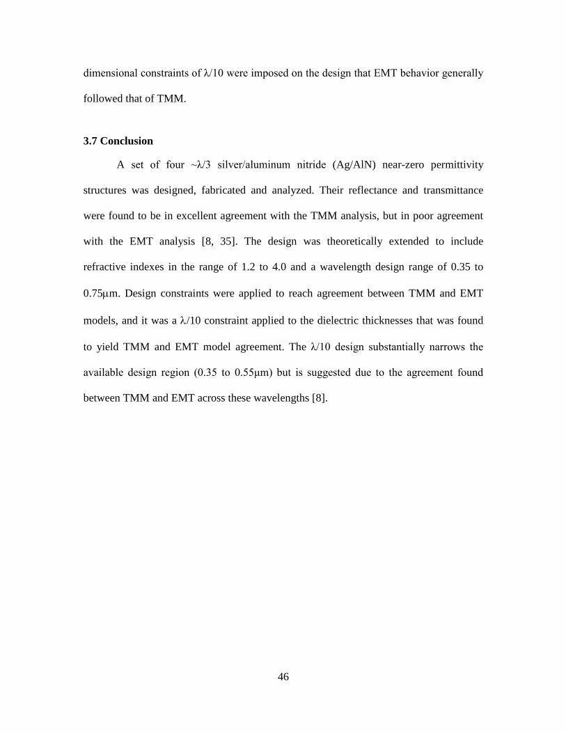
46
dimensional constraints of λ/10 were imposed on the design that EMT behavior generally
followed that of TMM.
3.7 Conclusion
A set of four ~λ/3 silver/aluminum nitride (Ag/AlN) near-zero permittivity
structures was designed, fabricated and analyzed. Their reflectance and transmittance
were found to be in excellent agreement with the TMM analysis, but in poor agreement
with the EMT analysis [8, 35]. The design was theoretically extended to include
refractive indexes in the range of 1.2 to 4.0 and a wavelength design range of 0.35 to
0.75µm. Design constraints were applied to reach agreement between TMM and EMT
models, and it was a λ/10 constraint applied to the dielectric thicknesses that was found
to yield TMM and EMT model agreement. The λ/10 design substantially narrows the
available design region (0.35 to 0.55μm) but is suggested due to the agreement found
between TMM and EMT across these wavelengths [8].

47
IV. OPTIMIZING A DUAL ROTATING RETARDER FOR A TUNABLE MUELLER MATRIX POLARIMETER-SCATTEROMETER
This chapter covers the dual-rotating-retarder (DRR) optimization methodology
used in the development of the tunable mid-wave infrared (MWIR) Mueller matrix (Mm)
polarimeter-scatterometer. The “Mm” term precedes polarimeter-scatterometer to infer
the polarimetric system used is a DRR [46]. The content of this chapter has been
submitted for publication in Measurement Science and Technology Journal in November
2012 [30]. The primary research contributions include: developing a method to predict
how well a particular DRR configuration will perform as a function of measurement
number; determining the Fourier retarder rotation scheme (5ω:1ω) is optimal when
oversampling is conducted; and leads into Chapter 5, where the first Mm scatterometer
having an optimal 1/3 wavelength (λ/3) retarder configuration was developed.
4.1 Executive Summary of Research
The value of Mueller-matrix (Mm) scatterometers lies in their ability to fully
characterize the polarimetric properties of samples. To extend their use to infrared (IR)
optical metamaterials requires tunable lasers and an achromatic dual rotating retarder
(DRR). The optimization methods used to develop the first tunable IR Mm scatterometer,
which uses an achromatic ~λ/3 retardance-configured DRR, are reported in this chapter.
The optimization process used is rooted in applying random error analysis to three
different DRR retardance configurations (λ/5, λ/4, and λ/3) with three different retarder
rotation ratios (θA:θG = 34:26, 25:5 and 37.5:7.5) and a variable number of intensity
measurements. The product of the error analysis was the level of error that could be

48
expected from a free-space Mm extraction when physical (retardance) and operational
(retarder rotation ratio and number of intensity measurements) specifications of the DRR
are made. The DRR specifications found optimal were a λ/3 retardance configuration and
a Fourier rotation ratio, with the number of measurements to collect dependent on the
level of error acceptable to the user. Experimental results corroborate the error analysis
findings with the achromatic ~λ/3 retardance-configured DRR consistently reaching 1%
error in the free-space Mm extractions.
4.2 Introduction
Mueller-matrix (Mm) scatterometers are of increasing interest for their ability to
determine the full-polarimetric behavior of materials/samples under test [59-65]. The
polarimetric engine of these instruments is a dual rotating retarder (DRR), and, for low-
error Mm extractions to be achieved, the retarder retardances should be on the order of
λ/4 to λ/3 and a calibration method should be used to remove systematic errors [39, 40,
66, 67]. High-quality optics and a robust alignment procedure are assumed when using a
DRR.
The retardance specification, λ/4 to λ/3, was made, in general, because of the
enhanced error performance that occurs when going from λ/4 to λ/3 and the poor error
performance for retardances less than λ/4. These performance features may be inferred
by condition number analysis [43] but become readily apparent under the random error
analysis applied in this chapter. Condition number analysis was used as a starting point in
the tunable infrared (IR) DRR optimization process. It was used to find low condition
number retarder rotation ratios when matched with λ/5, λ/4 and λ/3 retardance
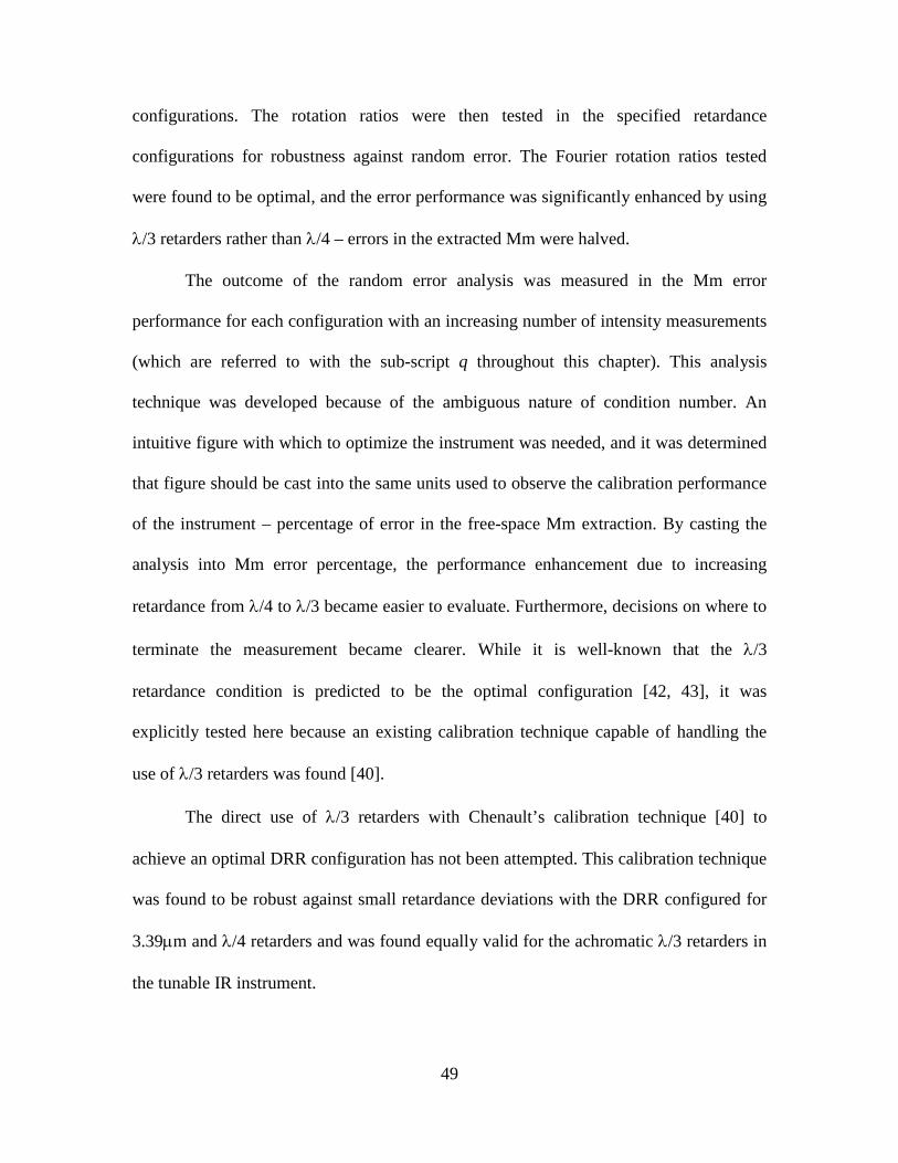
49
configurations. The rotation ratios were then tested in the specified retardance
configurations for robustness against random error. The Fourier rotation ratios tested
were found to be optimal, and the error performance was significantly enhanced by using
λ/3 retarders rather than λ/4 – errors in the extracted Mm were halved.
The outcome of the random error analysis was measured in the Mm error
performance for each configuration with an increasing number of intensity measurements
(which are referred to with the sub-script q throughout this chapter). This analysis
technique was developed because of the ambiguous nature of condition number. An
intuitive figure with which to optimize the instrument was needed, and it was determined
that figure should be cast into the same units used to observe the calibration performance
of the instrument – percentage of error in the free-space Mm extraction. By casting the
analysis into Mm error percentage, the performance enhancement due to increasing
retardance from λ/4 to λ/3 became easier to evaluate. Furthermore, decisions on where to
terminate the measurement became clearer. While it is well-known that the λ/3
retardance condition is predicted to be the optimal configuration [42, 43], it was
explicitly tested here because an existing calibration technique capable of handling the
use of λ/3 retarders was found [40].
The direct use of λ/3 retarders with Chenault’s calibration technique [40] to
achieve an optimal DRR configuration has not been attempted. This calibration technique
was found to be robust against small retardance deviations with the DRR configured for
3.39µm and λ/4 retarders and was found equally valid for the achromatic λ/3 retarders in
the tunable IR instrument.

50
4.3 Theory
4.3.1 Background
There are two approaches to conducting Mm analysis with DRRs. The first
approach is the measurement matrix method, which was optimized by Smith [43]. Here,
the retarder rotation ratio having the lowest condition number is suggested for conducting
the Mm measurement. Determining the number of measurements to collect is also
facilitated through condition number analysis. The second approach is the Fourier method
[41] which allows the user to select from a set of rotation increments satisfying the
5ω:1ω (analyzer retarder:generator retarder) rotation ratio, but the generator retarder must
incur a half or full rotation to complete the Mm measurement. This establishes the
number of measurements required to complete a Mm measurement.
The fundamental mathematical relationship for each of these methods is the same.
A set of intensity measurements is collected with a 4-element Stokes vector representing
the polarization state generator (PSG) stage and a 4-element row-vector representing the
polarization state analyzer (PSA) stage. Between the two matrices resides the Mm of the
sample to be analyzed. This is shown in Eqn. (4-1), where the g column-vector represents
the PSG, the a row-vector represents the PSA and q is the measurement number [46].
1,11 12 13 14
2,21 22 23 24,1 ,2 ,3 ,4
3,31 32 33 34
4,41 42 43 44
* *
q
qq q q q q
q
q
gm m m mgm m m m
I a a a agm m m mgm m m m
=
(4-1)

51
Every matrix equation can be consolidated into a summation of elements, as
shown in Eqn. (4-2). This is used as leverage to separate the measurement variables from
the Mm of the sample in both the measurement matrix and the Fourier method.
4 4
, , ,1 1
* *q q i i j j qj i
I a m g= =
= ∑∑ (4-2)
4.3.2 Measurement Matrix Method
The measurement matrix method is grounded in linear algebra where the impetus
is to mathematically isolate the Mm of the sample. This is accomplished by first
reorganizing the summation from Eqn. (4-2) into the following form [46].
4 4 4 4
, , , , , ,1 1 1 1
q q i j q i j q i j i jj i j i
I a g m w m= = = =
= =∑∑ ∑∑ (4-3)
From this, the W-matrix emerges, formulated by collecting the aq,i and gj,q elements.
When the W-matrix is multiplied by a vectorized Mm of the sample, the intensity
measurement can be constructed.
11
12
,11 ,12 ,13 ,14 ,21 ,44 13
44
.q q q q q q q
mm
I w w w w w w m
m
=
(4-4)
Simplifying this further, the measured intensities are seen to be a collection of row
operations performed by the measurement matrix (w-matrix) on the vectorized Mm of the
sample.
qI WM= (4-5)
The Mm can simply be solved as

52
1qM W I−= (4-6)
where W-1 is the inverse or pseudoinverse, depending on whether the measurement space
was oversampled or not.
Although not directly shown, the W-matrix is a function of retardances, δG and
δA, and the angular rotations, θG and θA, of the retarders. The row-dimension of the W-
matrix is dependent on the number of intensity measurements collected, q. Each of these
variables is used in the condition number analysis process.
4.3.3 Condition Number Analysis.
To achieve the least error in the extracted Mueller matrix, the W-matrix must be
well-conditioned. The condition number of the W-matrix infers its level of invertibility,
with a value of one indicating a completely invertible matrix and infinity indicating a
singular matrix. The condition number of the W-matrix is found according to
1( ) || |||| ||,pseudocond W W W −= (4-7)
where the infinity norm is used for the W-matrix and its inverse (or pseudo inverse when
oversampling is conducted) [43].
The traditional way to find the optimum retarder rotation ratio is to generate a
condition number plot [43] where the measurement number, q, and retardance values, δG
and δA, are kept constant, but the angular rotations of the retarders, θG and θA, are
allowed to vary. The global minimum (if one exists) represents the optimum retarder
rotation ratio. Three retardance cases were encountered during the development of the
tunable IR Mm scatterometer (δG = δA = λ/5, λ/4 and λ/3) and those values are used
throughout the analysis. The condition number plots found in Figure 4-1 represent the

53
analyzed retardance extremes (λ/5 on the left and λ/3 on the right) when 48
measurements are collected, and the angular rotations of the retarders (θG on the x-axis
and θA on the y-axis) were allowed to vary from 0.2 to 90o. The λ/4 case was not
included because there was not a large, perceivable difference between the λ/4 and λ/3
plots. The deep red regions refer to high condition numbers (singularities), while the blue
regions refer to low condition numbers. The difference in condition number between the
blue regions of the two plots is approximately an order of magnitude. Once a retarder
rotation ratio is settled upon, the optimum number of measurements to collect can be
examined by holding θG and θA, as well as δG and δA, constant and allowing q to vary.
Figure 4-1. Condition number plot for DRR under a 48-measurement collection configured with a λ/5 (a) and λ/3 (b) retarder. The x-axis refers to angular increments applied to the generator retarder, and the y-axis analyzer retarder increments.
4.3.4 Fourier Method
The constraints on the Fourier method are more stringent. It requires λ/4 retarders,
limits the retarder rotation ratio to 5ω:1ω, and necessitates that the PSG retarder incurs a

54
half or full 360o rotation. The first limitation is relaxed with the assistance of Chenault’s
calibration technique [40], which allows the Fourier ratio to be extended to include the
use of λ/3 retarders and reach the optimal retardance for a DRR [42, 43].
The basis of the Fourier method for DRR operation refers back to Eqn. (4-2) and
(4-3). The difference is now that the w-variable only takes on forms compatible with the
5ω:1ω rotation ratio and a q-dimension that forces the first retarder to complete a half or
full rotation cycle over the measurement process [40]. The uniqueness of this ratio is that
the Mm is encoded on the Fourier coefficients of the measured intensity signal.
Specifically, they are encoded on twelve harmonics contained in the measured signal.
This allows the signal, Iq, to be specified as a Fourier series according to [40]
12
01( cos(2 ) sin(2 )).q j q j q
jI a a j b jθ θ
=
= + +∑ (4-8)
This leads to a set of equations where the Mm elements can be uniquely determined as a
function of the Fourier coefficients [40, 46]. Corrections to the Mm elements are needed
when systematic errors are present.
4.3.5 Calibration Method
Chenault’s calibration technique [40] was an extension of Goldstein’s [39]. It
relies on specifying retardance errors in the PSG (δ1) and PSA retarders (δ2), and
alignment errors in the PSG (ε3) and PSA retarders (ε4) and analyzer (ε5). The error terms
can be found by conducting a free-space measurement. They are then used to correct
systematic errors in succeeding measurements. The strength of this calibration method is
in its span of corrections. It is capable of correcting measurements with retardance
deviations within λ/8 of the nominal λ/4 and misalignments up to 22.5o [40].

55
When working with this calibration technique, the retardance and alignment
errors were used to update the W-matrix used in the measurement matrix. This allowed
the error of the free-space measurement to be tracked as a function of the intensity
measurement. This type of analysis is not directly available to the Fourier method, since
Mm results are only available at the conclusion of a full or half rotation of the PSG
retarder. Updating the W-matrix with the values obtained from the calibration analysis
can also used to analyze non-Fourier rotation ratios tested. However, it is expected that
some systematic error will remain unaccounted for due to the presence of beam wander.
These effects are immune to the Fourier rotation ratios so long as a full 360o rotation of
the PSG retarder is applied [40]. An update of the W-matrix using the retardance and
alignment deviations found from the calibration measurement is used in the experimental
analysis in Section 4.4.4 to track the Mm error measurement by measurement for the
tested configurations.
4.4 Error Analysis
Conducting an error analysis on a particular DRR configuration is the most
intuitive/effective way to determine its robustness against random errors. Condition
number analysis is a good starting point. It provides a numerical result in the form of a
condition number for a particular DRR setup. However, the correspondence between
condition number and the error limitation of the chosen measurement parameters is not
immediately clear. This makes it difficult to make an informed decision when selecting
the retarder rotation ratio, retardances and the number of intensity measurements to
collect.

56
Error analysis was performed by introducing random errors to numerically created
ideal free-space intensity measurements. The deviation of the random error was kept
constant while the parameters of the measurements were varied. By comparing the
changing parameter values to the changing error in the resulting Mm’s, it was possible to
equate parameter selection to the error limitation of the system. The goal of this analysis
was to determine the best retarder rotation ratio to use and identify the performance
enhancement achieved by increasing the retardance.
4.4.1 Optimal Retarder Rotation Ratios
With the retarder restrictions established (λ/5, λ/4 and λ/3), condition number
analysis was used to find the optimal retarder rotation ratios to consider. Once found, the
ratios would be kept constant, while the retardance of the DRR configuration was varied.
The already-determined optimal rotation ratio found for 16 measurement case, 34:26,
[43] and two Fourier rotation ratios, 25:5 and 37.5:7.5, which were consistently found
among the lowest condition numbers with condition number analysis were used in the
optimization analysis. The condition number plots for each of the retardance cases are
shown in Figure 4-2.
The condition number findings are significant. They showed drastic changes for
the Fourier rotation ratios at the 17-measurement and 28-measurement marks for the
37.5:7.5 and 25:5 rotation ratios, respectively. The condition number performance for
each of the Fourier rotation ratios quickly surpassed the 34:26 rotation ratio performance.
Of additional interest is the convergence of the condition numbers of all three rotation
ratios as the retardance is increased. This analysis alone suggests the rotation ratios might

57
be irrelevant for oversampling with λ/3 retarders, but should definitely be considered, as
should the number of measurements, when operating a DRR with λ/4 or λ/5 retarders.
Figure 4-2. Condition number plot for the retardance cases tested (a) λ/5 (b) λ/4 and (c) λ/3 for the retarder rotation ratios 34:26, 37.5:7.5 and 25:5.
4.4.2 Creating ideal, free-space intensity signals
An ideal W-matrix (ideal polarizers, ideal retarders and perfect alignment) was
created for each test case, and then multiplied by the identity matrix to obtain the ideal,
free-space intensity signals. A snapshot of the free-space intensity signals for the 34:26,
25:5 and 37.5:7.5 retarder rotation ratios are shown in Figure 4-3, which show the
expected intensity waveforms for the three retardance conditions. These waveforms were
produced, so small, random errors could be introduced to them – to replicate the
introduction of random errors in the experimental measurement process.
4.4.3 Introducing random noise
All instruments suffer from the influences of random noise. In this case, the level
of random noise can be tested by examining the differences in the intensity measurements
from run to run. This was determined from a series of eight free-space measurements and
the aid of the following equation

58
1, ,
1, (%) 100%,
q p q
q q
I II
Average Measured Intensity Errorq
−
=∑
(4-9)
where q represents the intensity measurement number and p refers to the Mm
measurement series. The first measurement (I1,q) was used as the reference measurement,
from which average intensity deviations were determined from the seven measurements
Figure 4-3. Ideal free-space intensity signal under three different DRR retardance conditions (λ/5, λ/4 and λ/3) when the retarders are rotated under a ratio of (a) 34:26, (b) 37.5:7.5 and (c) 25:5.

59
that followed. The range of intensity deviations spanned 0.4% to 1.2%. A mid-range
value of 0.8% random error in the intensity measurement was used for the analysis to
remain in a representative range of the instrument.
The random function in MATLAB® allowed me to introduce random errors to
the ideal, free-space intensity signals described in Section 4.4.2. The syntax for the
random function is random(‘distribution type’,µ,σ,m,n), where µ represents the mean, σ
represents the standard deviation, m is the row size, and n is the column size of the
generated random error matrix. A normal distribution type was used. The mean (µ) was
set to one. The standard deviation (σ) was set to 0.01 because it led to errors in the
intensity signal that were consistent with the experimental set-up. Random errors were
introduced to the ideal free-space intensity signal and then the level of error in the
modeled intensity according to Eqn. (4-10). These operations were conducted 1,000 times
and then averaged. The standard deviation value was adjusted until 0.8% was reached,
replicating conditions similar to our experimental results.
, / ,
1 , (%) 100%
qIdeal i Idealw noise i
i Ideal i
I II
Average Modeled Intensity Errorq
=
−
=∑
(4-10)
To cast this analysis into a Mm error performance for each configuration and
track it on a measurement-by-measurement basis, a Mm extraction was performed against
the noisy intensity signal during each iteration of the loop. The error in the Mm extraction
was determined during each loop iteration according to

60
(%) 100%,free space extracted
free space
M MMm Error
M−
−
−= (4-11)
where the Mm for free-space was the identity matrix and the Mm for the measurement
represents the extracted Mm during each loop iteration. The Mm error for all the 1,000
iterations was found at the conclusion of the loop and is represented in the final results
plotted in Figure 4-4 for each of the tested configurations.
Figure 4-4. Expected error in the free-space Mm extraction for the rotation ratios, θA:θ G = 34:26 (blue), 25:5 (green) and 37.5:7.5 (red) using the three retardance restrictions (a) δ=λ/5, (b) λ/4 and (c) λ/3 and varying the number of intensity measurements (q) when additive random errors were introduced to ideal modeled intensity measurements for the DRR configuration represented.
The error analysis findings were also significant. They illustrate behaviors similar
to the condition number plots. The 37.5:7.5 Fourier rotation ratio performance exceeds
the 34:26 optimal rotation ratio at the 19-measurement point, two measurements later
than this occurred in the condition number plots. The 25:5 Fourier rotation ratio
performance exceeds the 34:26 rotation ratio at 28 measurements, the same measurement
point predicted by the condition number analysis. Trends with increasing measurement
number are even more significant now, however. There are slopes in the Mm error plots,

61
despite plateaus reached in the condition number plots of Figure 4-2. This illustrates the
need to perform measurements in excess of the number predicted from finding a stable
condition number. Additionally, the slope of the Mm error plots diminishes with
increasing retardance, with the overall minimum achievable error found in the λ/3
retardance configuration and the 37.5:7.5 Fourier rotation ratio. This is not necessarily
surprising, but what is strongly evident from this error analysis is that retardances less
than the commonly used λ/4 are increasingly susceptible to high errors in the Mm
extractions despite applying optimized rotation ratios and increasing the number of
intensity measurements. Thus, retardances less than λ/4 should generally be avoided.
Finally, the error performance of the λ/3 retardance configuration generally improved by
a factor of 2 over the λ/4 retardance configuration.
4.4.4 Experimental Results
With the DRR configured with ~λ/3 retarders (actually 110o at the 5.0µm
wavelength tested), two calibration measurements were made using the 25:5 and 37.5:7.5
rotation ratios. The systematic errors for the two measurements (δ1, δ2, ε3, ε4, ε5)
extracted from these measurements were in agreement with one another and were used to
update the W-matrix for Mm extractions using the measurement matrix method. This
technique permitted the Mm error for the three rotation configurations to be
experimentally compared.
Five free-space Mm measurements were collected on each of the three rotation
ratios (34:26, 25:5 and 37.7:7.5) following the calibration measurements described above.
The intensity measurements were averaged, and the free-space Mm was extracted from

62
the averaged intensity measurement. The average errors were determined as a function of
measurement number using the measurement matrix method with the updated W-matrix
in order to compare experimental results with the modeled results. Each is shown in
Figure 4-5, where the modeled results are represented by the solid curves and the
experimental values by the line with the ‘o’ markers.
Figure 4-5. Comparison of (a) modeled error in the free-space Mm extraction with the (b) experimental error for the instrument configured with ~λ/3 retarders in the DRR for three rotation ratio configurations (θA:θG = 34:26, 25:5 and 37.5:7.5).
Overall, the experimental and modeled 37.5:7.5 and 25:5 rotation-ratio results
agree well, while the 34:26 rotation-ratio experimental results do not achieve as low of
errors as predicted by the model. Intensity measurements in excess of 50 were collected.
The reduction in error continued for the 34:26 case, reaching 3.3% by measurement 58.
The 25:5 rotation ratio followed similar trends, where 1.1% error was achieved by
measurement 73. As mentioned in Section 4.3.5, the non-Fourier rotation ratio could have
systematic errors unaccounted for – due to beam wander. The Fourier rotation ratios
remain immune to these effects because the PSG retarder was rotated a full 360o [40]

63
during the calibration measurement and succeeding free-space measurements. Despite the
differences, it is clear that the 37.5:7.5 rotation configuration is the preferred
measurement arrangement to minimize the error in the extraction and to minimize the
number of measurements required to extract the Mueller matrix.
4.5 Discussion
From the analysis steps used to develop a tunable IR Mm scatterometer, the two
primary DRR measurement techniques were thoroughly reviewed along with the
available calibration methodologies. Early experimental work showed that low retardance
(λ/5), low measurement numbers (q<30), the measurement matrix method of operation at
θG:θA = 34:26, and the lack of a robust calibration technique led to large errors in free-
space Mm extractions. These results led to the examination of condition number
performance in greater detail and a method to translate condition number to a familiar
figure (percentage of error in the free-space Mm extraction) was realized. This analysis
was found to follow the condition number results when a random error on the order of
0.8% of the measured signal was applied to an ideal free-space intensity signal. The
anticipated Mueller errors were 3%, 2% and 1.5% for a DRR with 110o retarders, 50
measurements collected, and retarder rotation conditions of 34:26, 25:5 and 37.5:7.5,
respectively. Experimental results generally followed the analytical trends for the Fourier
compatible rotations, but the experimental data from the 34:26 rotation configuration was
found to be higher than the modeled predictions.
The use of λ/3 retarders in the final design was a direct impact of the availability
of a calibration technique capable of accommodating retardance deviations in excess of

64
30o [40], with the added benefit of optimizing the instrument and reducing the error in the
Mm extractions. The Fourier rotation ratios were found to be a favorable configuration
when performing condition number analysis of oversampled measurements. Each of
these was considered a key finding of this work, and led to the successful development of
a ~λ/3-retardance-configured tunable IR Mm scatterometer.
4.6 Conclusion
By evaluating the available range for Chenault’s calibration technique [40], it was
determined that a λ/3 design was possible. By applying condition number analysis and
random error analysis to free-space intensity signals represented by three different
retardance configurations (λ/5, λ/4 and λ/3) and three optimal rotation increments (34:26,
37.5:7.5, and 25:5), the Fourier method of DRR operations with λ/3 retarders was
determined to be the optimal DRR design configuration [28-30]. A tunable IR Mm
polarimeter-scatterometer configured with an achromatic ~λ/3-retardance-configured
DRR was ultimately designed, which now achieves low-error free-space Mm extractions
[30]. The completion of these optimization steps led to the development of the Mm
polarimeter-scatterometer described in the next chapter.

65
V. DEVELOPMENT OF A TUNABLE MID-WAVE INFRARED MUELLER MATRIX POLARIMETER-SCATTEROMETER
This chapter covers the development of the Mueller matrix (Mm) polarimeter-
scatterometer, which was completed following the findings from the dual rotating
retarder (DRR) optimization steps discussed in the previous chapter. The primary
research steps covered in this chapter include: introducing tunable infrared (IR) external-
cavity quantum cascade lasers (EC-QCLs) to an existing complete angle scatter
instrument (CASI®); establishing retarder design criteria for the implementation of an
achromatic dual rotating retarder (DRR) compatible with the EC-QCLs; confirming the
operational performance of the instrument with free-space calibration runs; and collecting
measurements on an IR metamaterial to validate the design intent. The results of this
research are in draft form with a planned submission to Review of Scientific Instruments
[31] and represents an instrument that is unique on a world-wide scale.
5.1 Executive Summary of Research
Optical metamaterials often have narrow-band performance features. At infrared
(IR) wavelengths, these features have only been observable with broad-band instruments
at specular angles and under a limited polarimetric evaluation due to the constraints of
existing instruments. A wavelength-tunable IR Mueller-matrix (Mm) polarimeter-
scatterometer which can tune on and off of narrow-band regions of interest and perform a
full polarimeteric and directional evaluation of IR metamaterials was developed. The
instrument is capable of performing these investigations at specular angles (acting as a

66
Mm polarimeter) and off-specular (acting as a Mm scatterometer), and opens the door to
fully evaluating optical metamaterials at IR wavelengths.
5.2 Introduction
Theoretical predictions of optical metamaterials show that the effective material
parameters of interest, typically electric permittivity and magnetic permeability, will
often depend on the incident angle and polarization of the incident radiation [9]. Also, the
attribution of optical phenomena observed or predicted for these materials, e.g., to Bragg
resonance as opposed to constitutive, homogeneous (effective) material parameters,
based on inclusion size and periodicity may not be clear-cut [4, 8]. Finally, these optical
phenomena, often based on Bragg or plasmonic resonances, are often narrow-band in
nature [10, 11]. An instrument that is capable of measuring infrared (IR) metamaterial
samples and providing a unique data set which, upon analysis, can lend significant insight
into each of these issues [68, 69].
The narrow-band performance features of optical metamaterials are most readily
found using a broadband instrument. A spectrometer can provide reflectance and
transmittance data for samples at normal or fixed, specular incident angles. When
increasing the measurement space to include polarization-sensitive measurements, a
variable-angle spectroscopic ellipsometer (VASE) can provide these data at varying
specular incident angles. The VASE can provide full, polarimetric analysis at visible and
near infrared (NIR), but in the infrared (IR) the IR-VASE can only provide a limited
polarimetric evaluation – it is capable of conducting co- and cross-polarization (ss, pp, sp,
ps) measurements and partial Mueller-matrix (Mm) extractions. For full polarimetric

67
characterization of samples at IR wavelengths at both specular and off-specular angles
(both in and out of the plane of incidence), an IR Mm polarimeter-scatterometer is
needed. This type of instrument was developed by using tunable external-cavity
quantum-cascade lasers (EC-QCLs), and it is now being used to evaluate the behavior of
optical metamaterials.
Scatterometers were once restricted to a small number of fixed-IR-wavelength
laser sources, but wavelength-tunable EC-QCLs have extended the range of wavelengths
offered to polarimeters and scatterometers. A series of tunable Daylight Solutions® EC-
QCLs were selected to span a nearly continuous range of mid-wave IR (MWIR, 4.37-
6.54µm) and long-wave IR (LWIR, 7.41-9.71µm) wavelengths, which were added to the
existing 3.39µm HeNe laser and 10.6µm CO2 laser in a Schmitt Measurement Systems
(SMS) Complete Angle Scatter Instrument (CASI®). Extensive hardware and software
upgrades were also implemented to introduce an achromatic dual rotating retarder (DRR)
polarimeter and accompanying rotation stages to the instrument. The end product is a
tunable IR Mm polarimeter-scatterometer, which can be tuned into and out of narrow-
band performance regions of optical metamaterials, allowing for the investigation of their
full range of directional scalar and polarimetric behaviors.
5.3 Instrument
5.3.1 Physical Layout
The CASI® already had an existing and suitable beam train for the introduction
of the EC-QCLs. Slight modifications were made so the EC-QCLs could be introduced
and easily aligned, which included the first turning mirror (TM) and beam combiner (BC)

68
shown schematically in Figure 5-1. The beam combiner was used to place a visible
alignment source in the beam path, and the turning mirror was used to couple an EC-QCL
into the beam path. More importantly, the turning mirror provides the means to bring the
EC-QCL into co-alignment with the system following the visible source alignment.
The co-alignment process is facilitated by power adjustments to the EC-QCL.
This allows thermal paper to be used to trace the IR beam through the system from source
to the detector, which is shuttered until a proper power level is restored. The end result of
the alignment process is the ability to visually verify the location of the IR source for
sample placement on the goniometer, and it provides the ability to adjust/determine the
rotational center of the sample after mounting it.
Figure 5-1. Physical layout of the Mueller matrix scatterometer using the following labeling conventions: TM – turning mirror; BC – beam combiner; Ch – chopper; PH – pinhole; FL – focusing lens; OAP – off-axis parabolic mirror; GP – generator-stage polarizer; GR – generator-stage retarder; AR – analyzer-stage retarder; AP – analyzer-stage polarizer.
5.3.2 EC-QCLs
A set of six EC-QCLs was selected to provide a continuous span of MWIR
wavelengths from 4.37 to 6.54µm and LWIR wavelengths from 7.41 to 9.71µm. Table 5-
1 shows the tunable range of each EC-QCL, their peak wavelengths and their peak

69
powers. Unlike gas lasers, the power of the EC-QCLs is adjustable, which is effective for
alignment, overall improvement of signal detection and achieving the highest dynamic
range of the instrument. The output powers of the 3.39µm HeNe and 10.6µm CO2 lasers
are 3.7mW and 14.6 W, respectively.
Table 5-1. EC-QCLs selected for the Mm polarimeter-scatterometer EC-QCL wavelength
range (µm) Peak λ (µm) Peak Power (mW)
4.35-4.55 4.5 220 4.74-5.15 4.9 160 5.16-5.67 5.3 330 5.76-6.54 6.1 280 7.40-8.23 7.8 340 8.06-9.71 8.8 5
The wavelength tuning ranges of the sources were tested using a Bristol 721B
spectrum analyzer and found to have excellent wavelength stability with bias. The sample
set of results shown in Table 5-2 demonstrates that the tuned-to-measured wavelength
deviation is correlated to the tuned wavelength rather than being strongly dependent on
the applied bias current. In general, the EC-QCL wavelength is able to be set to six
significant digits with relative uncertainty of less than 0.2%, and laser line-widths are less
than 30MHz CW and 30 GHz pulsed.
Table 5-2. EC-QCL wavelength stability performance under different bias conditions
EC-QCL tuned wavelength (µm)
Measured wavelength (µm) Deviation (µm)
5.76362 (500mA) 5.75113 0.01249 5.84300 (450mA) 5.83217 0.01083 6.08300 (400mA) 6.07669 0.00631 6.53586 (450mA) 6.53673 -0.00087 6.53586 (500mA) 6.53673 -0.00087

70
Automated wavelength tuning of the EC-QCLs is not a particular capability of the
instrument at this time. Scatterometers require stringent alignment. The EC-QCLs
grating-tune the wavelength, which creates enough beam walk that, when translated over
the length of the optical path, adjustments to the alignment are required.
5.3.3 Achromatic Dual Rotating Retarder Polarimeter
The most complex element of this instrument is the achromatic dual rotating
retarder (DRR). Extensive up-front analysis was conducted to determine the best retarder
rotation configurations and the optimal retardance configuration [28-30], both of which
leverage an existing calibration method [40]. Low-error, Mm extractions are only
possible with a robust calibration methodology. It was concluded that the (5ω:1ω)
Fourier rotation scheme [41] was optimal by applying condition number and error
analysis [30]. The Fourier rotation scheme traditionally uses λ/4 retarders, but it was
found that Chenault’s calibration methodology [40] could also be used for the optimal
λ/3 retardance configuration [42, 43].
Achromatic, nominally λ/3, CdS/CdSe wave-plates were obtained from Gooch
and Housego LLC for both the 4.3-6.5µm and 7.4-10.6µm wavebands. The predicted
retardance for the waveplates is shown in Figure 5-2. Actual retardance values range
from 109-116o. Four high-precision Aerotech, Inc. AGR-50 rotary stages were added and
electronically integrated to the CASI instrument to achieve the DRR configuration. The
AGR-50 has an internal 50:1 angular reduction ratio giving a calculated, repeatable step
size of 0.016o when driven by a 0.8o increment stepper motor [68, 69]. This is well within
the 0.3o accuracy recommended by Goldstein [46].
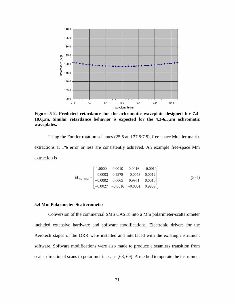
71
Figure 5-2. Predicted retardance for the achromatic waveplate designed for 7.4-10.6µm. Similar retardance behavior is expected for the 4.3-6.5µm achromatic waveplates.
Using the Fourier rotation schemes (25:5 and 37.5:7.5), free-space Mueller matrix
extractions at 1% error or less are consistently achieved. An example free-space Mm
extraction is
1.0000 0.0010 0.0016 0.00190.0003 0.9978 0.0053 0.0012
.0.0002 0.0065 0.9951 0.00100.0027 0.0016 0.0051 0.9969
free spaceM −
− − − = − − − −
(5-1)
5.4 Mm Polarimeter-Scatterometer
Conversion of the commercial SMS CASI® into a Mm polarimeter-scatterometer
included extensive hardware and software modifications. Electronic drivers for the
Aerotech stages of the DRR were installed and interfaced with the existing instrument
software. Software modifications were also made to produce a seamless transition from
scalar directional scans to polarimetric scans [68, 69]. A method to operate the instrument

72
as a polarimeter by conducting Mm measurements of a sample at specular angles as the
sample is rotated through a series of incident angles was implemented.
To illustrate the capabilities of the instrument, Mm results from a novel optical
metamaterial, which is a spectrally, directionally and polarimetrically selective absorber
[33], are shown with the instrument behaving as a Mm polarimeter and a Mm
scatterometer. With the instrument tuned to 5.0µm, the impetus for building this
instrument is clearly demonstrated – to investigate the polarimetric content of resonant
and off-resonant narrow-band features of optical metamaterials at specular and off-
specular angles of interest.
5.4.1 Mm Polarimeter Experimental Results
The CASI® Mm polarimeter was first set to collect specular reflectance over a
solid angle of 27msr-1 (i.e. diameter aperture at 0.5 m distance) at incident angles 15-65o,
with 1o increments collected near the resonant condition 20-30o and 5o increments outside
this region. Figure 5-3 shows the Mm results in the traditional 4x4 Mm format but where
each element is now a plot of the behavior of that element as a function of
incident/reflectance angle. The m00 element shows the first measurement collected at
each incident angle, and thus can generally be interpreted as a co-polarization (pp) Bi-
Directional Reflectance Distribution Function (BRDF) value. In this case, the presence of
a resonant feature in this optical metamaterials at 5µm and an incident angle of 25o is first
observed in the m00 element. The resonant feature which is incident angle dependent in
this material is clearly observed throughout the Mm elements and is only accessible with
the wavelength tunability of this instrument.

73
Figure 5-3. Mm specular reflectance plot for a novel optical metamaterial sample [33] at 5.0µm when the instrument was operating as a Mm polarimeter. I.e. in specular mode such that the angles represent both incident and reflected angle.
5.4.2 Mm Scatterometer Experimental Results
The same optical metamaterial [33] was examined with the CASI® Mm
scatterometer set at incident angles of 25o, the resonant condition observed for this
sample in Fig. 5-3, and at 60o, which represents an off-resonant condition. Figures 5-4
and 5-5 represent these measurements, respectively. As a scatterometer, the instrument
collects Mm BRDF, so the angles shown for each Mueller element represent the in-plane
reflectance angle for that particular incident angle. At the specular angle (represented by
0o in each of these figures), the same information shown in Figure 5-3 at 25o is shown
again here. Away from specular, diffraction orders can be observed, indicating that this
sample was fabricated in “tiles” approximately 140µm in size (the mask size of this
particular electron-beam lithography process) and “tiled” together in a square lattice to
form the larger sample. The polarization content of the light scattered by this sample is

74
Figure 5-4. Mm BRDF of a novel optical metamaterial sample [33] at 5.0 µm and 25o incident angle. The resonant feature of Figure 5-3 is repeated here. The periodic structure is diffraction orders generated by the periodic nature of the sample. superimposed on this diffraction pattern. In Figure 5-5, the information in Figure 5-3 at
60o (where the resonant feature is absent) is again shown here at 0o (i.e. specular).
Likewise, diffraction orders similar to those of Figure 5-4 and the superposition of
polarimetric information on these orders are again observed here.
Figure 5-5. Mm BRDF of a novel optical metamaterial sample [33] at 5.0 µm and 60o incident angle, illustrating the off-resonant condition. The diffraction orders seen in Figure 5-4 are again found here.

75
5.5 Discussion and Conclusion
Analyses of directional and polarimetric characteristics of narrow-band features
found among optical metamaterials at IR wavelengths have been limited by limited data
observable through the use of broad-band instruments only at specular angles and under
limited polarimetric conditions. With the introduction of the tunable IR Mm polarimeter-
scatterometer, narrow-band features found among optical metamaterials can be more
fully explored, both at specular and off-specular (both in and out of the plane of
incidence). Significant up-front analysis allowed this instrument to be designed and built
in the optimal DRR configuration, which was discussed in the previous chapter [28-30].
The free-space results shown in this chapter demonstrate terrific calibration performance.
The example results for an optical metamaterial sample illustrated the ability of this
instrument to provide unique spectral, polarimetric and directional information on these
samples.
This instrument was developed to deliver an unmatched ability to collect and
analyze the behavior of IR optical metamaterials. This chapter demonstrated the
collection abilities of the instrument. The analytical techniques to apply to the measured
results are the focus of the next chapter.

76
VI. EVALUATION OF A NOVEL OPTICAL METAMATERIAL ABSORBER
This chapter covers the novel measurements collected on an infrared (IR)
metamaterial absorber (MMA) [33], using the tunable IR Mueller matrix (Mm)
polarimeter-scatterometer described in Chapter 5. Modeling and subsequent polarimetric
analysis was performed on the Mm extracted for the MMA. The findings from these
analyses are covered in this chapter and demonstrate original, unpublished work with a
planned submission to Applied Physics Letters.
6.1 Executive Summary of Research
Resonant MMAs are of interest for their selective impedance matching abilities to
free-space. The periodic surface structures and non-transmissive backplane, which are
separated by a dielectric layer, are responsible for their novel resonant absorbing
characteristics [17]. While these resonances are designed features, surface wave
resonances have also been found in these structures outside of the intended design
regions. These resonances can have incident angle and polarization dependencies, which
are observable with complete polarimeters where their polarimetric behaviors are
captured in the form of a Mueller matrix (Mm). When in this form, example polarimetric
behavior of the material can be examined with the introduction of Stokes-defined
polarization states for either a Stokes vector analysis or a Poincaré sphere representation
of the reflected state(s) – each was conducted as a part of this research. Mm modeling is
also available and can be used to extract polarization-relevant information which is
responsible for unique polarization signatures.

77
The Mm model of a Fresnel reflector having a complex refractive index is well-
known [37], and manifests a unique Mm signature consisting of polarization magnitude
and retardance features. They resemble polarizer-like features in the Mm elements, m00,
m01, m10 and m11, and retardance features in the Mm elements, m22, m23, m32 and m33. The
Mm extracted for the MMA was found to follow these characteristics, had low
depolarization and a distinct polarization resonance. The resonant feature was found not
to follow basic Fresnel reflectance models, even when modeling constraints were relaxed
to uniaxial anisotropy ( x y zn n n= ≠ ) and biaxial anisotropy ( x y zn n n≠ ≠ ) conditions. The
extracted reflectance magnitude and phase behavior is real; however, the MMA does not
behave as an effective medium.
6.2 Introduction
A resonant, spectrally selective MMA was studied [33]. To examine polarization
spectral and incident angle dependencies, a broad-band infrared variable angle
spectroscopic ellipsometer (IR-VASE) was first used to collect p-polarization (p-pol) and
s-polarization (s-pol) reflectance spectra. The MMA was designed to resonantly absorb
optical radiation in regions centered around ~6.3 µm and ~8.2 µm. These resonant
absorption valleys were reconfirmed, but a strong, surface plasmon polariton (SPP)
resonance intersecting 5.0µm and 25o incident angle was also observed. To the best of
my knowledge, a full polarimetric evaluation of an SPP mode remains unreported at this
time.
The Mm polarimeter [31] was tuned to 5.0µm for the collection of the Mm of this
sample. The collected Mm was first confirmed physically realizable. Then, it was

78
analyzed according to a Mm reflectance model, where the behavior of the reflectances
(Rs and Rp) as well as the phase behavior between the s-pol and p-pol states is
determined. From these extractions, it remains convincing that effective complex
refractive index values for this material are not expected. Although the extracted Mm
shows evidence of Fresnel reflectance behavior of a material having a complex refractive
index for the s-pol reflectance (Rs), it remains clear that the periodic nature of the
material produces resonant reflectance magnitude and phase characteristics which are not
reproducible even when the model is relaxed to biaxial conditions. Following the Fresnel
analysis, example behaviors of the sample against canonical polarization states (linear
horizontal, linear 45o and right hand circular) are reviewed. The chapter closes with the
ellipticity (χ) and orientation (ψ) calculations of the reflected polarization states (linear
+45 and right hand circular) for a Poincaré sphere interpretation.
6.3 IR VASE Measurements
With the IR-VASE, both p-pol and s-pol measurements can be collected for a
sample over a range of incident angles from 25o to near grazing. Complex refractive
index data can be retrieved for layered samples, when the thicknesses of the individual
layers are known. Similarly, the material thicknesses can be determined in the instance
the complex refractive index data of the sample is known [70]. Neither of these options
remains available for non-homogeneous materials because well-known models linking
the structure of the sample to the complex reflectance spectra do not exist [70]. Thus, this
instrument was leveraged in this research to find a polarimetric region of interest, where

79
the Mm polarimeter could be used to recover the full-polarimetric details of a
metamaterial sample.
An SPP mode centered at 5.0µm and 25o incident angle was found for the novel
MMA sample [33]. The IR-VASE p-pol and s-pol spectra are shown in Figure 6-1, where
the p-pol spectrum is on the left and s-pol spectrum is on the right. The measurement
angles span those which are observable with the Mm polarimeter, with the exception of
the lower incident angle. The IR-VASE can only reach 25o, but the Mm polarimeter can
reach 15o. Thus, the polarimetric state of the sample could be observed with the Mm
polarimeter for incident angles 15-25o, near the SPP mode at 25o and at angles greater
than 25o.
Figure 6-1. (left) P-pol and (right) s-pol reflectance measurements taken of the MMA with increasing incident angle using the IR-VASE
The IR-VASE measurements show two absorption resonances which are
stationary with respect to incident angle at ~6.3µm and ~8.2µm, and two resonances
whose resonant wavelengths are incident angle dependent. The mechanism responsible
for the incident angle dependent absorption resonance in the s-pol spectra remains

80
undetermined at this time. The absorption resonance in the p-pol plot is due to an SPP
mode, which can be found from solving
,SPP x xk k jg= ±
(6-1)
where kx refers to the in-plane propagation vector ( 0 sin( )x ik k θ=
), with k0 referring to
the free-space propagation constant, and xg refers to the grating vector ( 2 /xg aπ= , with
a referring to the periodic spacing between the surface features) [71, 72]. The mode order
is specified by j. The first order (j = 1) SPP resonance is encountered when Eqn. (6-1) is
satisfied and can be rewritten as
0 0
2 2 2sinSPPi
na
π π πθλ λ
= ±
. (6-2)
This equation is solved for λ0 and plotted as a function of incident angle in Figure 6-2 to
show the incident angle behavior of the predicted SPP resonance. The material properties
in ñSPP for the MMA (Au and the dielectric spacer) were specified at 5.0µm [71, 72].
Au spacerSPP
Au spacer
nε ε
ε ε=
+
(6-3)
The periodic spacing was a = 3.2µm. An expected SPP resonance was found at 5.2µm at
a 25o incident angle, which is close to the experimentally observed resonance occurring at
5.0µm and 25o.

81
Figure 6-2. Surface plasmon polariton resonance calculated for the MMA, using the material properties of Au at 5.0µm (ñ = 3.7+ i30.5) [34] and the dielectric (ñ = 2.06 +0.12) [17], while the periodic spacing a= 3.2µm.
6.4 Mm Polarimeter Measurements
The Mm polarimeter was configured to collect specular reflectance measurements
at 5.0µm for incident angles from 15 to 65o. Increments of 1o were used from 20 to 30o
and increments of 5o were used outside of the resonant feature. Figure 6-3 shows the
extracted specular reflectance Mm for the MMA. There is clear evidence of the SPP
resonance, peaking in the vicinity of 25o.
Figure 6-3. Normalized specular reflectance Mm plot for the MMA at 5.0µm.

82
The behavior of the Mm illustrates both polarizer and retarder tendencies, where the
polarizer tendencies are found in the m00, m01, m10 and m10 terms, and the retarder
tendencies are found in the m22, m23, m32 and m32 terms.
6.5 Determining the Mm is physically realizable
Before performing modeling analysis with the extracted specular reflectance Mm
for the MMA sample, it had to first be determined physically realizable. The trace of the
Mm multiplied by its transpose must adhere to following inequality [46].
3
2 200
, 0( ) 4 ,ij
i jTr m m
=
= ≤∑TMM (6-4)
where M refers to the extracted Mm of the sample and MT is its transpose. The equality
applies to a non-depolarizing sample, while the inequality infers the presence of
depolarization. Verifying this equality ensures the degree of polarization requirement of
the outgoing Stokes vector is met, where the degree of polarization of a Stokes vector is
[46]
2 2 2
1 2 3
0
1.S S S
DOPS
+ += ≤ (6-5)
The extracted Mm for the MMA was found to be physically realizable, with only
minor depolarization, which was primarily present at the resonant peak. This is shown in
Figure 6-4. The values outside of the resonance were 0.98 to 0.99 and the lowest value in
the resonant region was 0.96. Overall, the sample was found to be very polarization
preserving and its Mm physically realizable.
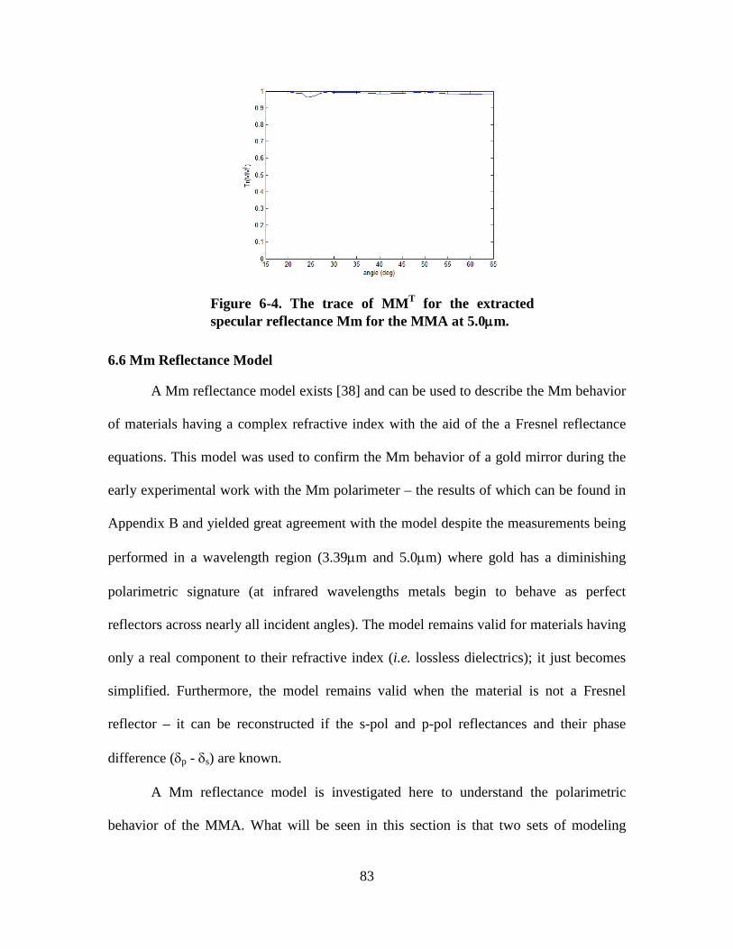
83
Figure 6-4. The trace of MMT for the extracted specular reflectance Mm for the MMA at 5.0µm.
6.6 Mm Reflectance Model
A Mm reflectance model exists [38] and can be used to describe the Mm behavior
of materials having a complex refractive index with the aid of the a Fresnel reflectance
equations. This model was used to confirm the Mm behavior of a gold mirror during the
early experimental work with the Mm polarimeter – the results of which can be found in
Appendix B and yielded great agreement with the model despite the measurements being
performed in a wavelength region (3.39µm and 5.0µm) where gold has a diminishing
polarimetric signature (at infrared wavelengths metals begin to behave as perfect
reflectors across nearly all incident angles). The model remains valid for materials having
only a real component to their refractive index (i.e. lossless dielectrics); it just becomes
simplified. Furthermore, the model remains valid when the material is not a Fresnel
reflector – it can be reconstructed if the s-pol and p-pol reflectances and their phase
difference (δp - δs) are known.
A Mm reflectance model is investigated here to understand the polarimetric
behavior of the MMA. What will be seen in this section is that two sets of modeling

84
considerations must be examined to extract information from the measured Mm, that is,
the un-normalized Mm (raw measurements which are in a Fourier described BRDF
space) and the normalized Mm, for which results are cast into Mueller space having a
range from -1 to +1.
6.6.1 Un-normalized Mm Reflectance Model
The un-normalized Mm of a general reflector has the following form [38]
0 00 01 .0 0 2 cos( ) 2 sin( )2
0 0 2 sin( ) 2 cos( )
s p s p
s p s p
Rs p p s s p p s
s p p s s p p s
R R R RR R R R
M R R R R
R R R R
δ δ δ δ
δ δ δ δ
+ − − +
= − − − − − − −
(6-6)
where Rs and Rp can refer to the Fresnel reflectances for s-pol and p-pol light, and δs and
δp refer to the phases gained upon reflection for the s-pol and p-pol light, which come
from the following Fresnel amplitude equations [70].
20
0
20
0
sin( )cos( ) 1
sin( )cos( ) 1
s
ii
is s
ii
nn nn
r r enn n
n
δ
θθ
θθ
−
− − = = + −
(6-7)
20
0
20
0
sin( )1 cos( )
sin( )1 cos( )
p
ii
ip p
ii
nn nn
r r enn n
n
δ
θ θ
θ θ
−
− − = = − +
(6-8)
It is here that we see if a complex refractive index (ñ = n - iκ) exists, there will be a
unique phase for both the s-pol and p-pol light, whose effects will show up in the m22,
m23, m32 and m33 terms. In the instance the refractive index is purely real (i.e. dielectric, ñ
= n) and under external reflection, the phase difference between the s-pol and p-pol
reflectances are 0o or 180o. In this case, the m23 and m32 terms evaluate to zero, and the

85
Mm takes on the form of a polarizer [46]. On a final note, the Fresnel intensity
reflectances (Rs and Rp) can be found from
2
s sR r= (6-9)
and
2.p pR r= (6-10)
From this model, the following relationships among the elements of the un-
normalized Mm can be used to obtain the behavior of the s-pol and p-pol reflectances.
11 01sR m m= − (6-11)
01 11pR m m= − (6-12)
These reflectances were extracted from the measured data and then scaled to agree with
the 25o reflectance data collected from the IR-VASE measurements. Great agreement
between the two sets of results can be seen in Figure 6-5. Scaling was required because
this data was in BRDF space (sr-1), and the polarimetric measurements were collected
with an over-sized aperture since rotating optical elements are in the beam train. In short,
this means direct access to the Rs and Rp measurements are not available but the overall
Figure 6-5. Rs (green) and Rp (blue) reflectance behaviors determined from un-normalized Mm data for the MMA at 5.0µm. Markers represent reflectance data from the IR-VASE measurement.

86
behavior can be. What is immediately evident is that the Rp behavior is not indicative of
an effective complex refractive index for an isotropic material. Later it will be shown that
the Rs behavior generally follows the behavior of gold at infrared wavelengths.
6.6.2 Normalized Mm Reflectance Model
Since the measurements were collected in BRDF space, the Mm requires
normalization. This is facilitated by dividing all the Mm elements by the measured m00 or
m11 term, which are identical. This scales the Mm to values relevant to Mm’s (-1 to +1).
It is the normalized form of the Mm that is reported in literature and is the form of the
Mm reported in Figure 6-3 for the MMA. Note the form of m00 has been changed in the
representation of Figure 6-3 (it is the BRDFpp). The normalized Mm reflectance model is
of the following form.
_
0 0
0 0
.2 cos( ) 2 sin( )
0 0
2 sin( ) 2 cos( )0 0
s p s p
s p s p
s p s p
s p s p
R nmeass p p s s p p s
s p s p
s p p s s p p s
s p s p
R R R RR R R RR R R RR R R R
MR R R R
R R R R
R R R RR R R R
δ δ δ δ
δ δ δ δ
+ − + + − +
+ + =
− − − −
+ + − − − + +
(6-13)
When normalized, direct access to the Rs and Rp is no longer available; however, a ratio
of the reflectances can be established from a series of operations performed with the Mm
elements.
00 _ 01_2 s
nmeas nmeass p
Rm mR R
+ =+
(6-14)

87
00 _ 01_
2 pnmeas nmeas
s p
Rm m
R R− =
+ (6-15)
00 _ 01_
00 _ 01_
nmeas nmeas p
nmeas nmeas s
m m Rm m R
−=
+ (6-16)
Eqn. (6-16) is plotted in Figure 6-6 (top plot) and could be used in an attempt to find the
complex refractive index of the MMA if the functional form of the reflectances is known.
Also shown in Figure 6-6 is the phase difference between the p-pol and s-pol
states. This can be found from using either the un-normalized or the normalized Mm
according to,
1 23
22
tan .p smm
δ δ − − =
(6-17)
Figure 6-6. Ratio of the reflectances (top) and phase difference between the p-pol and s-pol reflectances (bottom).

88
6.6.3 Fresnel Reflectance Comparisons
Qualitative comparisons between three Fresnel reflectance models (isotropic,
uniaxial anisotropic, or biaxial anisotropic) are made here to investigate the polarimetric
behavior of the MMA, in particular, the exotic Rp behavior.
Isotropic: Example Fresnel reflectance and phase behavior of gold (the patterned
metal on the surface of the MMA) is shown in Figure 6-7 for two different wavelengths
(0.2µm and 5.0µm). These two wavelengths were selected to show the disparity in the
character of gold in the ultraviolet (near its plasma frequency) and at the wavelength at
which the MMA sample was examined. In each case, it can be seen that a loss index (κ)
prevents the Rp curve from reducing to zero (i.e. there is no Brewster angle for a material
having a complex refractive index) but there is a general Fresnel reflectance character to
each of the polarization states. What can also be seen is that a large loss index encourages
high reflectivity from both the s-pol and p-pol states and diminishes the discrimination
between them (until high incident angles are reached). This material property also leads
to a lack of phase discrimination between the two polarization states. The phase behavior
generally follows the discrimination between of the two polarization states. The Rs
reflectance curve of the MMA looks similar to the Rs reflectance curve for gold at
infrared frequencies. However, the Rp Fresnel reflectance curve does not follow the
behavior of gold in the infrared. Overall, it can be expected that an isotropic model will
not predict the MMA’s Rp behavior.

89
Figure 6-7. Modeled Fresnel reflectance and phase curves for gold (surface material of MMA) at 0.2µm (a) and (b) (ñ = 1.427 + i1.215) and 5.0µm (c) and (d) (ñ = 3.7 + i30.5).
Uniaxial anisotropic: The isotropic comparisons/findings are not surprising.
Many metamaterials are considered anisotropic, since they often do not meet the unit cell
or inclusion constraints that would allow an effective media description at their design
wavelength [4]. The amplitude Fresnel reflectance equations for uniaxial anisotropic
materials are [70] when ñx = ñy
2 2
_ 2 2
cos( ) sin ( )
cos( ) sin ( )i y i
s anisotropic
i y i
nr
n
θ θ
θ θ
− −=
+ −
(6-18)
and
2 2
_ 2 2
cos( ) sin ( ).
cos( ) sin ( )x z i z i
p anisotropic
x z i z i
n n nr
n n n
θ θ
θ θ
− −=
+ −
(6-19)

90
For the uniaxial case, ñx is assumed to be equal to ñy, while ñz is allowed to vary
according to the resonant design. Exotic behaviors can be seen when a large variation in
ñz is available (but may not be physically realizable). Figure 6-8 illustrates example
findings. The complex refractive indexes for nx and ny were held constant at values
representative of gold at 5.0 µm (n = 3.7, κ = 20.5), while values for ñz where tested for
resonant behavior. Behavior similar to the MMA’s Rp could not be replicated.
Figure 6-8. Modeled Fresnel reflectance curves for an anisotropic uniaxial material, where nx = ny = 3.7, κx = κy = 30.5, nz = 3 (a), 0.3 (b), 0.03 (c), and 0.003 (d) κz = 0.01.
Biaxial anisotropic: With two sets of complex refractive indexes to vary (ñy was
held constant while ñx and ñz were varied), resonant behavior similar to those seen in the
MMA data was obtained. But, like the previous modeling results, these are only of
qualitative value. Figure 6-9 illustrates the resonant feature found from this modeling.
The biaxial model is not expected to work either because the resonance in the measured
Rp is attributed to an SPP resonance rather than from an effective medium.

91
Figure 6-9. Predicted Fresnel reflectances using an anisotropic biaxial model (nx = 0.03, κx = 0.05, ny = 3.7, κy = 30.5, nz = 0.45, κz = 0.01).
6.7 Example Behavior of the MMA
6.6.1 Stokes Interpretation
Three reflected Stokes vectors are shown in Figure 6-10, where (a) is from
applying a linear horizontal polarization state (s-pol), (b) is from a linear +45o state and
(c) is from a right-hand-circular (RHC) polarization state. When the linear horizontal
state is incident on the MMA, a linear horizontal state is returned. This trivial case is
presented to illustrate the m11 term of the measured Mm can be used to determine this
behavior and will always be unity for a Fresnel-type reflector. When a linear +45o state is
incident, a left-handed elliptical state is produced (values are present in S1, S2 and S3),
which switches its rotation to right-handed at the resonance. The behavior of the elliptical
state over the full range of incident angles is more accessible in the Poincaré sphere
analysis presented in the next section. When the RHC state is incident, a left-hand
elliptical state is produced with resonant behavior at the SPP mode.

92
_
1100
in LHS
=
_ 45
1010
in LS
=
_
1001
in RHCS
=
Figure 6-10. Stokes plots for the MMA when canonical Stokes polarization states (a) horizontal (b) +45˚ and (c) right-hand circular are applied to the extracted Mm, with the respective incident Stokes vector shown below each plot.
6.7.2 Poincaré Sphere Interpretation
The Stokes vectors presented in the last section are inverted here to arrive at a
more direct approach to evaluating the reflected behavior of the polarization states
following the introduction of the linear +45o and RHC states. The relationship between
the Stokes-vector Poincaré-sphere angles’ ellipticity (χ) and orientation (ψ) are shown in
the following equation [46].

93
0
1
2
3
1cos(2 )cos(2 )cos(2 )sin(2 )
sin(2 )
S
SSSS
χ ψχ ψ
χ
= =
(6-20)
The value of the ellipticity (χ) is directly retrievable using S3.
( )1
3sin2
Sχ
−
= (6-21)
The orientation (ψ) can be found from the ratio of S2 and S1.
1 2
1
1 tan2
SS
ψ − =
(6-22)
Each of these angles is plotted for the linear +45o and RHC cases in Figures 6-11 and 6-
12.
Figure 6-11. The ellipticity (χ) and major axis orientation (ψ) of the reflected Stokes vector with linear +45o (left) and right hand circular (right) polarization states incident on the MMA at 5.0µm.

94
Figure 6-12. Traces of the reflected polarization states on the Poincaré sphere for the MMA when the incident wavelength is 5.0µm and the polarization state is linear +45o (left) and RHC (right).
6.8 Discussion and Conclusion
Measurements were conducted on an MMA with the Mm polarimeter to capture
the SPP behavior in Mm form. The instrument was tuned to 5.0µm and measurements
were collected at incident angles spanning 15-65o. The Mm extracted for the series of
incident angles was distilled into s-pol and p-pol reflectance behaviors and the phase
behavior found between the s-pol and p-pol reflectances. This was conducted so the
experimental results could be analyzed in the context of Fresnel reflectance models for
the isotropic, uniaxial anisotropic and biaxial anisotropic cases. It was determined that the
isotropic and uniaxial anisotropic models could not be used to replicate the resonant
behavior found in the p-pol reflectance data. And, while a resonant behavior could be
produced using a biaxial anisotropic model ( x y zn n n≠ ≠ ), a match to the measured data

95
could not be achieved. It is concluded that analyzing this MMA with an effective-
medium Fresnel reflectance model is not appropriate due to the SPP resonance resulting
from the MMA’s periodic structure. An appropriate reflectance model having a periodic
dependent description is required to simulate the measure results. Such a model should
also demonstrate the conservation of energy interpretation (like Fresnel) to fully predict
the Mm behavior of the sample.
Despite the lack of agreement between the measured data and the Fresnel
reflectance models, the extracted Mm is valid (physically realizable) and follows the Mm
reflectance model description. This said, example polarimetric reflectance behavior of the
MMA was examined, assuming a set of canononical polarization states (linear horizontal,
linear +45o, and RHC) were incident on the material. This was used to show the predicted
outgoing Stokes vectors and produce a Poincaré sphere interpretation of the reflected
polarization states. The effects of the resonant reflectance behavior as well as the phase
relationships between the s-pol and p-pol states were readily observed in this analysis.
This chapter demonstrated the modeling methodology and data distillation
process applied to the first IR optical metamaterial measured with the tunable IR Mm
polarimter-scatterometer. Future measurement efforts with this instrument are expected to
leverage from this analysis methodology. With this said, the next chapter reviews a
compilation of recent samples/materials from literature with unique behaviors in the
spectral range of this instrument and illustrate a non-exhaustive review of basic optical
physics research opportunities available due to the development of this instrument.

96
VII. FUTURE WORK
The Mueller matrix (Mm) polarimeter-scatterometer has demonstrated its ability
to produce a unique data set for the analysis of infrared (IR) metamaterials samples. This
instrument can be used to perform basic optical physics research of IR metamaterials and
any other materials developed for applications in the 4.35-9.71µm wavelength range.
Thus, this chapter is dedicated to identifying future work, as many novel materials are
being developed in the spectral range of the tunable IR Mm polarimeter-scatterometer.
7.1 Metamaterial Absorbers
Metamaterial absorbers (MMAs) are among some of the most recent mid-wave IR
(MWIR) and long-wave IR (LWIR) material developments. The Mm polarimeter-
scatterometer has already been used to characterize the polarimetric behavior a MMA at
5.0µm [33]. However, there are several other architectures which have recently been
developed and reside in the spectral range of the Mm polarimeter-scatterometer. Figure
7-1 shows the results of a theoretical study for materials designed for high absorption at
infrared frequencies, where unit cell structure dimensions as well as dielectric thicknesses
were modified to examine the predicted absorption behavior of these structures [74]. In
Figure 7-2 and 7-3, two separate experimental MMA developments are shown which
operate in for near the spectral domain of the Mm polarimeter-scatterometer. In Figure 7-
2, a MMA was designed to have wide-band absorption from 3-12µm [75]. In Figure 7-3,
a multiplexed MMA was designed for resonant absorption ~3.5 µm [76] but could easily
be modified to reach the spectral range of the instrument using guidance from [74].

97
Figure 7-1. Theoretical MMA design (top) where the available unit cell dimensions are varied to show the expected changes in the resonant response [74].
Figure 7-2. A wide-band MMA design (left) with its measured absorption (right) [75].

98
(a) (b) (c) Figure 7-3. A non-multiplexed (a) and multiplexed (b) MMA design with the measured reflectance (c) [76].
7.2 Releasable IR Metamaterials
The concept of releasable IR metamaterials came from the need to deposit
spectrally selective structures on a non-planar surface [77]. Much of the metamaterial
work has been directed at developing resonant structures on substrates and thereby
restricting their use to planar surfaces. These materials are in a unique research domain,
and the Mm polarimeter-scatterometer has the spectral range to characterize them.
Figure 7-4. Scanning electron microscope (SEM) image of releasable IR metamaterial flakes (left) and the spectral reflectance (right), with the right axis depicting the measured results for the flakes [77].

99
7.3 Photonic Crystals
Photonic crystals represent yet another material with IR designs found in the
spectral range of the Mm polarimeter-scatterometer. Figure 7-5 shows a three-
dimensional photonic crystal made from tungsten having a photonic bandgap over the
range of 8-20µm and strong absorption at 6µm near the band edge [78].
Figure 7-5. SEM image (left) for a photonic crystal made of tungsten, which demonstrated a photonic bandgap over 8-20µm [78].
7.4 Dielectric Resonators
Dielectric resonators have been recently introduced to metamaterials as a means
of achieving optical magnetism with low-ohmic loss. Figure 7-6 shows the fabricated
cubic dielectric array with its novel reflectance and transmittance spectra [79].
Figure 7-6. SEM image of cubic dielectric array (left) with the unique reflectance and transmittance spectra (right) [79].

100
7.5 Conclusion
A non-exhaustive review of recent publications was conducted, where numerous
materials have been developed for MWIR and LWIR wavelengths. Each of these
materials was shown to have unique reflectance and transmittance spectra where basic
optical physics research could be conducted on these materials with the use of the Mm
polarimeter-scatterometer. This serves as further validation to the relevance of
developing this one-of-a-kind instrument. Numerous collaboration opportunities are
anticipated, and this instrument is expected to bring about deeper, physical
understandings of these materials.

101
VIII. DISCUSSION AND CONCLUSIONS
8.1 Research Objective Restatement
The body of research covered in this document was directed at identifying and
solving problems affecting optical metamaterials research. A series of research objectives
was assembled to address the use of effective medium theory (EMT) in the simplest
structures of metamaterial research and address the absence of an instrument capable of
meeting the full-directional and full-polarization characterization demands of infrared
metamaterials.
• Model, design, fabricate and test an optical near-zero permittivity structure and identify the appropriate design constraints to apply for EMT usage in the design and post-fabrication analysis steps
• Develop an optimal dual rotating retarder (DRR) polarimeter which is compatible with mid-wave infrared (MWIR, 4.37-6.54µm) and long-wave infrared (LWIR, 7.41-9.71µm) wavelengths
• Develop the first tunable IR Mm polarimeter-scatterometer for the characterization of IR optical metamaterials
• Measure an IR metamaterial with the tunable IR Mueller matrix (Mm) polarimeter, determine the appropriate model needed to replicate the experimental results, and perform polarimetric analysis using canonical polarization states to describe the measured results
8.2 Research Objective Accomplishment
The research objectives in this research were primarily accomplished in a model,
design, and then experimentally verify approach. The first of which was identifying the
dimensional constraints necessary to bring EMT and transfer matrix method (TMM)
modeling into agreement for near-zero permittivity designs created from periodic, layered
metal-dielectric media. Four near-zero permittivity design structures with periods

102
numbering one to four and having a λ/3 design constraint were fabricated for this work,
and the TMM model was confirmed accurate for all four samples. The EMT model did
not accurately predict the reflectance and transmittance results for these structures. Using
TMM as the model truth source, design dimensions of the near-zero permittivity design
were reduced until evidence of model-to-model agreement was achieved – that
dimensional constraint was λ/10. The contributions from this research have been
accepted for publication in Optics Express [8].
The next problem confronted in this research was the development of a tunable IR
Mm polarimeter-scattterometer. This instrument was needed because of the lack of an
instrument having full-directional (specular, off-specular, in-plane, out-of-plane), full
polarimetric and the spectral range to robustly characterize IR optical metamaterials.
Targeting the IR was important for the early identification of problems in optical
metamaterials because the natural design progression is from the IR to visible
wavelengths. Initial efforts to develop this instrument commenced with beam train
modifications to an existing SMS CASI® and utilizing existing sets of λ/4 retarders
designed for 3.39 and 10.6µm wavelengths to implement a dual rotating retarder (DRR),
which is used to make the instrument a Mm polarimeter-scatterometer. The retarders,
initially on-hand, were found incompatible with the tunable EC-QCL sources from FTIR
measurements and random error analysis, which showed retardances below λ/4 led to
poor error performance of the instrument. This same error analysis was used to determine
the optimal retarder and retarder rotation ratio to apply to the instrument – retarders
having λ/3 retardance and rotated according to a Fourier method rotation ratio (25:5 or

103
37.5:7.5 were found optimal) [28-30]. The contribution from this research has been
submitted for publication in Measurement Science and Technology Journal in November
2012 [30].
The λ/3 retarders were not on-hand, so design specs were coordinated with Gooch
and Housego to produce two sets of achromatic λ/3 retarders. Obtaining stable retardance
and anti-reflective coatings is extremely challenging over the 4.35-9.71µm wavelengths
spanned by the EC-QCLs and it was important to maintain the retardances below 135o for
compatibility with an existing DRR calibration technique [40], so two sets were designed.
One spanned 4.35-6.5µm and the other set spanned 7.4-10.6µm; there was a natural break
in the EC-QCLs that facilitated a clean definition for the two sets of retarders. The CO2
laser wavelength was included in the span of the second set of retarders as an
improvement measure for the DRR at 10.6µm. When the λ/3 retarders were introduced to
the CASI®, they met the predictions of the random error analysis (~1% error in the free-
space measurement). The contributions of this research are in draft form with a planned
submission to the Review of Scientific Instruments [31].
While awaiting the delivery of the λ/3 retarders, work with the CASI® was
conducted at 3.39µm. It was while operating at this wavelength that Mm reflectance
modeling commenced. This model was first used to predict the Mm behavior of a gold
mirror at the 3.39µm operating wavelength. The modeling resumed once the λ/3 retarders
arrived, where Mm measurements were conducted at 5.0µm. Both sets of measurements
were in good agreement with the Mm reflectance model despite being conducted at IR

104
wavelengths where a gold mirror behaves as an ideal reflector at nearly all incident
angles. This model was later used to deduce the behavior of a MMA.
A unique MMA was measured with the tunable IR Mm polarimeter-
scatterometer. As a scatteometer, the tiled features stemming from the electron-beam
lithography mask used to design the material were evident, with strong diffractive results
seen in the Mm plots [31]. As a Mm polarimeter, the behavior of an SPP resonance was
observed when measurements were collected at 5.0µm and incident angles spanning 15-
65o. The SPP resonance was first seen in the broad-band IR-VASE measurement, as an
incident angle dependent resonance in the p-pol reflectance was observed. Phase
matching analysis was conducted to confirm the presence of an SPP mode. This analysis
predicted a 5.0µm SPP resonance near 25o incident angle, where the SPP mode was
found and the Mm that was extracted captured the polarimetric characteristics of an SPP
mode for the MMA.
The extracted Mm for the MMA was found to populate the Mm elements similar
to how a gold mirror would (a Fresnel reflector having a complex refractive index), with
the exceptions of stronger roll-offs with increasing incident angles and the resonant
feature coming from the SPP resonance. The behavior of the s-pol (Rs) and p-pol (Rp)
reflectances were distilled from the measured data as was the phase behavior between
these two polarization states. While Rs appeared similar to an isotropic Fresnel
reflectance, Rp did not. In any case, the models for Rs and Rp were assumed Fresnel-like
to perform analysis for the isotropic, uniaxial anisotropic and biaxial anisotropic cases –
in an attempt to replicate the resonant behavior found in Rp.

105
The isotropic and uniaxial anisotropic models were found incapable of producing
the resonant feature found in the Rp data. When the Fresnel model was relaxed to biaxial
anisotropic considerations, a resonant feature similar to the Rp could be attained, but a
match to the measured data could not be achieved. It is concluded that analyzing this
MMA with an effective-medium Fresnel reflectance model is not appropriate due to the
SPP resonance resulting from the MMA’s periodic structure. Thus, it is concluded that
Fresnel modeling could not be expected to replicate the Rp behavior accurately, and an
energy-conserving, periodic description of the material is necessary to predict the p-pol
reflectance and achieve Mm predictions for the MMA sample – and likewise will be
needed for future SPP resonant analysis.
Despite these Fresnel model findings, the Mm extracted for the sample was found
to be physically realizable and is valid. Thus, the extracted Mm for the MMA was used to
produce predictions for the polarimetric behavior of reflected Stokes vectors under
incident canonical Stokes states (or any Stokes-defined polarization state of interest). The
Stokes analysis also led to a useful Poincaré sphere interpretation for a visual depiction of
reflected states as a function of incident angle. The contributions from this research
represent original, unpublished work, which are planned submission to Applied Physics
Letters.
Table 8-1 provides a summary of the contributions from this research, which span
refereed journals, conference proceedings papers and conference presentations.

106
Table 8-1 List of Contributions
Refereed Publications
[8] Vap, J., Seal, M.D., Marciniak, M.A., Johnson, L. and Moran, M., “Practical design constraints for stratified optical near-zero effective permittivity structures,” accepted to Opt. Exp. (Nov 2012).
[30] Vap, J., Nauyoks, S. and Marciniak, M. A., “Evaluation and optimization of a tunable mid-wave infrared Mueller-matrix polarimeter-scatteromer,” Meas. Sci. and Tech, manuscript submitted 1 Nov 2012.
[31] Vap J., Nauyoks, S., Benson, M., Fitzgerald, T. and Marciniak, M.A., “Tunable infrared Mueller-matrix polarimeter-scatterometer for the evaluation of optical metamaterials,” manuscript prepared for submission to Rev. of Sci. Instr.
Vap J., Nauyoks, S. and Marciniak, M.A., “Full-polarimetric analysis of a metamaterial absorber,” preparing manuscript for submission to App. Phys. Lett.
Conference Proceedings
[28]Vap, J., Nauyoks, S., Fitzgerald, T. and Marciniak, M. A., “Development of a tunable polarimetric optical scattering instrument from 4.3-9.7 Microns,” Proc. SPIE 8154, 815412 (2011).
[29] Vap, J. Nauyoks, S. and Marciniak, M. A., “Optimization of a mid-wave tunable polarimetric optical scatter instrument,” Proc. SPIE 8364, 836405 (2012).
[34] Vap, J. and Marciniak, M.A., “Examining epsilon near zero structures through effective medium theory and optical thin film analysis,” Proc. SPIE 8364, 836426 (2012).
Presentations
“Development of a tunable polarimetric optical scattering instrument from 4.3-9.7 Microns,” SPIE Optics and Photonics Conference, San Diego, CA, Aug 2011.
“Optimization of a mid-wave tunable polarimetric optical scatter instrument,” SPIE Defense Sensing and Security Conference, Baltimore, MD, Apr 2012.
“Examining epsilon near zero structures through effective medium theory and optical thin film analysis,” SPIE Defense Sensing and Security Conference, Baltimore, MD, Apr 2012.

107
APPENDIX A
A.1 Complex Refractive Index Data
There are two sets of commonly used complex refractive index data for the
common noble metals referenced in metamaterial literature, Palik [36] and Johnson [37].
The common noble metals referred to are silver (Ag), gold (Au) and copper (Cu). Tabular
forms of these data can be found in the original publications and electronic forms can be
found at a refractive index website [73]. Comparisons of the data are shown in Figure A-
1. The general findings for Johnson’s Ag data were lower values for the real part and
higher values for the imaginary part of the complex refractive index.
Figure A-1. Comparison of complex refractive index data from Johnson [37] (a) and (c) Palik’s [36] (b) and (d) for the noble metals copper (Cu), gold (Au) and silver (Ag).

108
Differences between the data sets will obviously lead to differences in the
modeled reflectance and transmittance spectra. When using Johnson’s data for ENZ
modeling, it over predicted the transmission results that were experimentally achieved at
short wavelengths (long ultraviolet and short visible). It was originally believed due to
lower values for the imaginary component of the complex refractive index. The data of
Figure A-1 suggested otherwise – Johnson’s Im(ñ) data was actually higher than Palik’s.
Additionally found, the real component of the complex refractive index was found to be
lower in Johnson’s data than in Palik’s. What this suggests is that considering each of
these complex refractive index values in isolation at these wavelengths leads to erroneous
expectations (expected high reflectance for low Re(ñ) and low transmission for high
Im(ñ)). Thus, I turned to modeling to arrive at to arrive at what could be expected from a
30nm layer of Ag using the transfer matrix modeling discussed in Chapter 3. The
reflectance and transmittance spectra were calculated, and they were summed to illustrate
conservation of energy and to identify where absorption would take place. The results are
shown in Figure A-2.
Figure A-2. Modeled reflectance and transmittance spectra for a 30nm layer of Ag using the complex refractive index data from Johnson [37] (left) and Palik [36] (right).

109
A.2 Complex Permittivity Data
The relationship between the complex permittivity and the complex refractive
index at optical frequencies is
,n n iκ ε= + = (A-1)
where n refers to the refractive index and k refers to the absorption index. This leads to
the following relationships for the real and imaginary components of the complex
permittivity [1], which are plotted in Figure A-3 from bulk data [35,36].
2 2Re( ) nε κ= − (A-2)
Im( ) 2nε κ= (A-3)
Figure A-3. Comparison of complex permittivity data from Johnson [37] (a) and (c) and Palik [36] (b) and (d) for the noble metals copper (Cu), gold (Au) and silver (Ag).

110
These plots again show the differences in the bulk data. Figure A-4 is a zoomed in
view of the zero crossings for the permittivity of each of the noble metals each of which
exist at ultraviolet frequencies (below 0.4µm). When developing zero permittivity
structures for the visible frequencies using metal-dielectric layers, the design goal is to
dilute the permittivity with the introduction of a positive permittivity material (dielectric).
This pushes the zero permittivity to longer wavelengths, which will be observed in the
modeling and experimental results when proper scaling of the dielectric thicknesses are
adhered to [8].
Figure A-4. The real part of the complex permittivity from Palik’s data [36], which show the zero crossings.
A.3 Practical design constraints to achieve a near zero permittivity structure
The contents of Chapter 3 were directed at finding the practical design constraints
(dielectric thicknesses) to apply to a stratified composite metal-dielectric near-zero
permittivity design structure. The plot in Figure 3-2 (f) illustrated the design region which
should be targeted; this was the region were the best agreement between the transfer
matrix method (TMM) and effective medium theory (EMT) modeling occurred. Table A-
1 shows the design values for the perimeter of this figure (left hand side and the diagonal

111
running up the right hand side of the design region) as well as wavelengths in the heart of
the design region (0.4µm). The highlighted region in the table depicts the near-zero
permittivity design values for the Ag/AlN structures modeled and experimentally
examined in Chapter 3.
Table A-1. λ/10 design values tested for TMM and EMT agreement
fm(λ,n) fm fd td n λ
fm(2.0,0.35) 0.69 0.31 9.0nm 2.0 0.35µm
fm(3.0,0.35) 0.83 0.17 4.0nm 3.0 0.35µm
fm(4.0,0.35) 0.90 0.10 2.0nm 4.0 0.35µm
fm(2.0,0.4) 0.51 0.49 19.0nm 2.0 0.4µm
fm(3.0,0.4) 0.70 0.30 8.0nm 3.0 0.4µm
fm(4.0,0.4) 0.81 0.19 5.0nm 4.0 0.4µm
*fm(2.0,0.63) 0.20 0.80 80.0nm 2.0 0.63µm
fm(3.0,0.47) 0.56 0.44 16.0nm 3.0 0.47µm
fm(4.0,0.55) 0.60 0.4 14.0nm 4.0 0.55µm
*Actual values used in the ENZ design tested, which meet λ/3 design constraints rather than the λ/10 design constraints met among the points tested above.
A.4 TMM and EMT model agreement
The design values identified in Table A-1 were used to generate the TMM and
EMT plots found in Figures A-5 and A-6. Each plot in Figure A-5 shows good agreement
between the TMM and EMT modeling; this is generally because the design values fall
below the λ/10 constraint. What is seen among the 0.4µm designs is diminishing

112
agreement between the TMM and EMT models as the refractive index is increased.
Figure A-6 shows that the λ/10 constraint may require tightening up for designs using
large refractive index (n=4), as the agreement between the models above the design
wavelength begins to deteriorate.
Figure A-5. EMT to TMM modeling comparison of a four period structure at the design wavelengths of 0.35 and 0.4µm for the refractive indexes n=2, 3 and4.
Figure A-6. EMT to TMM modeling comparison of a four period structure at the design wavelengths 0.47 and 0.55µm for the refractive indexes n = 2.0 and n = 4.0, respectively.

113
APPENDIX B
B.1. Mueller Matrix Model for Fresnel Reflector – Gold Mirror
The Mueller matrix (Mm) for a gold mirror can be modeled according to the Mm
reflectance model covered in Chapter 6. The normalized Mm of Eqn. (6-13) is restated as
Eqn. (B-1) here.
_
0 0
0 0
2 cos( ) 2 sin( )0 0
2 sin( ) 2 cos( )0 0
s p s p
s p s p
s p s p
s p s p
R nmeass p p s s p p s
s p s p
s p p s s p p s
s p s p
R R R RR R R RR R R RR R R R
MR R R R
R R R R
R R R RR R R R
δ δ δ δ
δ δ δ δ
+ − + + − +
+ + =
− − − −
+ + − − − + +
(B-1)
The reflectance terms (Rs and Rp) refer to the s-polarized (s-pol) and p-polarized (p-pol)
Fresnel reflectances and phases (δs and δp) gained upon reflection. Each of these terms
are not repeated here but can be found in Eqns. 6-7 through 6-10. When the complex
refractive index (ñ) is used in these relationships, each of the elements in the reflectance-
defined Mm can be modeled. Figure B-1 and B-2 are used to illustrate the expected
behavior of the affected Mm elements for reflectance from a gold mirror as a function of
incident angle and wavelength. Figure B-1 just shows the m10 term, which is the same as
the m01 term. The m00 and m11 terms evaluate to unity and thus are not shown. Figure B-2
shows m22, m23, m32, and m33, which are the elements that show the retardance effects of
the gold mirror due to the phase differences between the reflected s-pol and p-pol states.

114
Figure B-1. The modeled m10 term of the normalized reflectance Mm for a gold mirror.
Figure B-2. The modeled m22, m23, m32, and m33 terms of the normalized reflectance Mm for a gold mirror.
From the modeled results it can be seen that there is not a strong signature in the
m10 term (and similarly the m01 term) at infrared wavelengths; however there are strong

115
differences between the s-pol and p-pol reflectances that lead to an observable signature
at the visible (0.4 to 0.7µm) and ultra-violet (0.2-0.4µm) wavelengths shown. Similar
effects can be seen in the Mm elements shown in Figure B-2, where there is not a strong
signature found at infrared wavelengths but strong signatures exist again at the visible
and ultra-violet wavelengths shown.
Mm measurements were collected of a gold mirror at 3.39µm and 5.0µm with the
Mm polarimeter and compared with the modeling results coming from the use of Eqn.
(B-1) and Palik’s bulk complex refractive index data for Au [36] at these wavelengths.
Comparisons between the measured and modeled results for the m22, m23, m32, and m33
elements are shown in Figure B-3. The other Mm elements are not shown because they
Figure B-3. Modeled-to-measured results comparison of the m22, m23, m32, and m33 elements of a Mm reflectance for a gold mirror at 3.39µm and 5.0µm.

116
evaluate to one or zero. Overall, good agreement between the modeled and measured Mm
for the gold mirror were found at 3.39µm and 5.0µm and provided the necessary
confidence in measurements collected from the Mm polarimeter to move forward with
measuring metamaterials.
B.2 Mm Polarimeter Measurements of Gold Mirror
The full Mm results from the gold mirror measurements collected at 3.39µm and
5.0µm are shown in Figure B-4 and B-5, respectively. To reiterate, the values found in
the Mm elements m22, m23, m32 and m33 of these two plots are shown in Figure B-3 for
the Mm reflectance model comparison.
Figure B-4. Mm plot for a gold mirror at 3.39µm.

117
Figure B-5. Mm plot for a gold mirror at 5.0µm.

118
BIBLIOGRAPHY
[1] Cai, W. and Shalaev, V., [Optical Metamaterials], Springer, New York (2010).
[2] Pendry, J., “Metamaterials in the sunshine,” Nature 5, 599-600 (2006).
[3] “Photonic Metamaterials.” Article on Photonic Metamaterials, Negativ-index Media, Negative Refraction, Cloaking. N.p., N.d. Web. 21 Nov. 2012. <http://www.rp-photonic.com/photonic_metamaterials.html>.
[4] Simovski, C.R. and Tretyakov, S.A., “Local constitutive parameters of metamaterials from an effective-medium perspective,” Phys. Rev. B 75, 195111 (2007).
[5] Soukoulis, C.M., Zhou, J., Koschny, T., Kafesaki, M. and Economou, E.N., “The science of negative index materials,” J. Phys: Condens. Matt. 20, 304217 (2008).
[6] Karri J. and Mickelson, A.R., “Silver dielectric stack with near-zero epsilon at a visible wavelength,” 2009 IEEE Nano. Matl. Dev. Conf., 148-53 (2009).
[7] Roberts, M.J., Feng, S., Moran, M. and Johnson, L., “Effective permittivity near zero in nanolaminates of silver and amorphous polycarbonate,” J. Nano. 4, 043511 (2010).
[8] Vap, J., Seal, M.D., Marciniak, M.A., Johnson, L. and Moran, M., “Practical design constraints for stratified optical near-zero effective permittivity structures,” accepted to Opt. Exp. (Nov, 2012).
[9] Menzel, C., Rockstuhl, C., Paul, T. and Lederer, F., “Retrieving effective parameters for metamaterials at oblique incidence,” Phys. Rev B 77, 195328 (2008).
[10] Jakoljecic, M.M., Isic, G., Basic, B., Oates, T.W.H., Hinrichs, K., Bergmair, I., Hingerl, K., and Gajic, R., “Spectroscopic ellipsometry of split ring resonators at infrared frequencies,” Appl. Phys. Lett. 100, 11105 (2012).
[11] Marciniak, M.A., Sellers, S.R., Lamott, R.B., and Cunningham, B.T., “Bidirectional scatter measurements of a Guided Mode Resonant Filter photonic crystal structure,” Opt. Exp. 20, 27242 (2012).
[12] Burckel, D.B., Wendt, F.R., Ten Eyck, G.A., Ellis, A.R., Brener, I. and Sinclair, M.B., “Fabrication of 3D Metamaterial resonator using self-aligned membrane projection lithography,” Adv. Matt. 22, 3171 (2010).
[13] Burckel, D.B., Wendt, J.R. Ten Eyck, G.A., Ginn, J.C., Ellis, A.R., Brener, I., and Sinclair, M.B., “Micrometer-scale cubic unit cell 3D metamaterial layers,” Adv. Matt. 22, 5053 (2010).

119
[14] Jiu, B., Wu, S., Li, J. and Gu, M., “Near-infrared high refractive-index three-dimensional inverse woodpile photonic crystals generated by a sol-gel process,” J. Appl. Phys. 102, 096102 (2007).
[15] Wu, C., Nuener III, B., John, J., Milder, A., Zollars, B., Savoy, S. and Shvets, G., “Metamaterial-based integrated plasmonic absorber/emitter for solar thermo-voltaic systems,” J. Opt. 14, 024005 (2012).
[16] El-Kady, I., Biswas, R., Ye, Y., Su, M.F., Puscasu, I., Pralle, M., Johnson, E.A., Daly, J. and Greenwald, A., “Tunable narrow-band infrared emitters from hexagonal lattices," Photonics and Nanostructures – Fundamental and Applications 1, 69 (2003).
[17] Watts, C.M., Liu, X. and Padilla, W.J., “Metamaterial electromagnetic wave absorbers,” Advanced Opt. Matl. 24, 98-120 (2012).
[18] Sai, H., Yugami, H., Kanamori, Y. and Hane, K., “Spectrally selective thermal radiators and absorbers with periodic microstructured surface for high-temperature applications,” Microscale Thermophysical Engineering 7, 101 (2003).
[19] Dahan, N., Niv, A., Biener, G., Gorodetski, Y., Kleiner, V. and Hasman, E., “Enhanced coherency of thermal emission: Beyond the limitation imposed by delocalized surface waves,” Phys. Rev. B 76, 045427 (2007).
[20] Dahan, N., Nic, A., Biener, G., Gorodetski, Y., Kleiner, V. and Hasman, E., “Extraordinary coherent thermal emission from SiC due to coupled resonant cavities,” J. Heat Transfer 130, 112401 (2008).
[21] Lin, S.Y., Moreno, J. and Fleming, J.G., “Three-dimensional photonic-crystal emitter for thermal photovoltaic power generation,” Appl. Phys. Lett. 83, 380 (2003).
[22] Luk, T.S., Mclellan, T., Subramania, G. Verley, J.C. and El-Kady, I., “Emissivity measurements of 3D photonic crystals at high temperatures,” Photonics and Nanostructures-Fundamentals and Applications 6, 81 (2008).
[23] Marquier, R., Joulain, K., Mulet, J.P., Carminati, R., Greffet, J.J. and Chen, Y., “Coherent spontaneous emission of light by thermal sources,” Phys. Rev. B 69, 155412 (2004).
[24] Sai, H., Yugami, H., Akiyama, Y., Kanamori, Y. and Hane, K., “Spectral control of thermal emission by periodic microstructured surfaces in the near-infrared region,” J. Opt. Soc. Am. A 18, 1471 (2001).

120
[25] Yeng, Y.X., Ghegrehan, M., Bermel, Pl, Chan, W.R., Joannopoulos, J.D., Soljacic and I. Celanovic, “Enabling high-temperature nanophotonics for energy applications,” PNAS 109, 2280 (2012).
[26] Le Gall, J., Olivier, M. and Greffet, J.J., “Experimental and theoretical study of reflection and coherent thermal emission by a SiC grating supporting a surface-phonon polariton,” Phys. Rev. B 55, 10105 (1997).
[27] O’Sullivan, F., Celanovic, I., Jovanovic, N., Kassakian, J., Akiyama, S. and Wada, K., “Optical characteristics of one-dimensional Si/SiO2 photonic crystals for thermophotovoltaic applications,” J. Appl. Phys. 97, 033529 (2005).
[28] Vap, J., Nauyoks, S., Fitzgerald, T. and Marciniak, M. A., “Development of a tunable polarimetric optical scattering instrument from 4.3-9.7 Microns,” Proc. SPIE 8154, 815412 (2011).
[29] Vap, J. Nauyoks, S. and Marciniak, M. A., “Optimization of a mid-wave tunable polarimetric optical scatter instrument,” Proc. SPIE 8364, 836405 (2012).
[30] Vap, J., Nauyoks, S. and Marciniak, M. A., “Evaluation and optimization of a tunable mid-wave infrared Mueller-matrix polarimeter-scatteromer,” Meas. Sci. and Tech, manuscript submitted 1 Nov 2012.
[31] Vap J., Nauyoks, S., Benson, M., Fitzgerald, T. and Marciniak, M.A., “Tunable infrared Mueller-matrix polarimeter-scatterometer for the evaluation of optical metamaterials,” manuscript prepared for submission to Rev. of Sci. Instr.
[32] Silveirinha, M. and Engheta, N., “Tunneling of electromagnetic energy through subwavelength channels and bends using ε-near-zero materials,” Phys. Rev. Lett. 97, 157403 (2006).
[33] Liu, X., Tyler, T., Starr, T., Starr, A.F., Jokerst, N.M., and Padilla, W.J., “ Taming the Blackbody with infrared metamaterials as selective thermal emitters,” PRL 107, 045901 (2011).
[34] Adams, D.C., Inampudi, S., Ribaudo, T., Slocum, D., Vangala, S., Kuhta, N.A., Goodhue, W.D., Podolskiy, V.A. and Wasserman, D., “Funneling light through a subwavelength aperture with epsilon-near-zero materials,” Phys. Rev. Let., 107 133901 (2011).
[35] Vap, J. and Marciniak, M.A., “Examining epsilon near zero structures through effective medium theory and optical thin film analysis,” Proc. SPIE 8364, 836426 (2012).
[36] E.D. Palik, [Handbook of Optical Constants], London-New York (1985).

121
[37] Johnson P.B. and Christy R.W., “Optical-constants of noble-metals,” Phys. Rev. B 6, 4370 (1972).
[38] Chipman, R.A., [Handbook of Optics, 3rd Edition], Chapter 14, McGraw Hill (2010).
[39] Goldstein, D.H. and Chipman, R.A., “Error analysis of a Mueller matrix polarimeter,” J. Opt. Soc. Am. A 7(4), 693-00 (1990).
[40] Chenault, D.B., Pezaniti, J.L. and Chipman, R.A, “Mueller matrix algorithms,” Proc. SPIE 1726, 231-46 (1992).
[41] Azzam, R.M.A, “Photopolarimetric measurement of the Mueller matrix by Fourier analysis of a single detected signal,” Opt. Lett. 2(6), 148-50 (1978).
[42] Sabatke, D.S., Descour, M.R., Dereniak, E.L., Sweatt, W.C., Kemme, S.A. and Phipps, G.S., “Optimization of retardance for a complete Stokes polarimeter,” Opt. Lett. 25, 802-04 (2000).
[43] Smith, M., “Optimization of a dual-rotating retarder Mueller matrix polarimeter,” Appl. Opt. 41, 2488 (2002).
[44] Stover, J. C., [Optical Scattering Measurement and Analysis], SPIE Press (1995).
[45] Schott, J.R., [Fundamentals of Polarimetric Remote Sensing], SPIE Press (2009).
[46] Goldstein, D., [Polarized Light], CRC Press (2003).
[47] Schubert, E.F., Kim, J.K. and Xi, J.-Q., “Low-refractive-index materials: A new class of optical thin-film materials,” Phys. Stat. Sol. B 244, 3002-08 (2007).
[48] Xi, J.-Q., Kim, J.K., Schubert, E.F., Ye, D., Lu, T.-M. and Lin, S.-Y., “Very low-refractive-index optical thin films consisting of an array of SiO2 nanorods,” Opt. Lett. 31, 601-03 (2006).
[49] Xi, J.-Q., Schubert, M.F., Kim, J.K., Schubert, E.F., Chen, M., Lin, S., Liu, W. and Smart, J.A., “Optical thin-film materials with refractive index for broadband elimination of Fresnel reflectance,” Nat. Photon. 1, 176-79 (2007).
[50] Grosso, D., Boissiére, C. and Sanchez, C., “Ultralow-dielectric-constant optical thin films built from magnesium oxyfluoride vesicle-like hollow nanoparticles,” Nat. Mat. 6, 572-75 (2007).
[51] Chi, F., Yan, L., Yan, H., Jiang, B., Lu, H. and Yuan, X., “Ultralow-refractive-index optical thin films through nanoscale etching of order mesoporous silica films,” Opt. Lett. 37, 1406-08 (2012).
122
[52] Schwartz, B.T., Piestun, R., “Waveguiding in air by total external reflection from ultralow index metamaterials,” App. Phys. Let. 85, 1-3 (2004).
[53] Brown, J., “Artificial dielectrics having refractive indices less than unity,” Proc. IRE 100C, 51-62 (1953).
[54] Rotman, W., “Plasma simulation by artificial dielectrics and parallel-plate media,” IRE Trans. Antennas Propag. 10, 82-95 (1962).
[55] Garcia, N., Ponizovskaya, E.V., and Xiao, J.Q., “Zero permittivity materials: band gaps at the visible,” Appl. Phys. Let. 80, 1120-22 (2002).
[56] Schwartz, B.T. and Piestun, R., “Total external reflection from metamaterials with ultralow refractive index,” J. Opt. Soc. Am. B 20, 2448-53 (2003).
[57] Edwards, B., Alù, A., Young, M. E., Silveirinha, M., and Engheta, N., “Experimental verification of epsilon-near-zero metamaterial coupling and energy squeezing using a microwave waveguide,” Phys. Rev. Let., 100, 033903 (2008).
[58] Born, M. and Wolf, E., [Principles of Optics], Cambridge University Press, New York (2006).
[59] Schiff, T. C., Stover, J. C., Bjork, D. R., Swimley, B. D., Wilson, D. J. and Southwood, M. E., “Mueller matrix measurements with an out-of-plane polarimetric scatterometer,” Proc. SPIE 1746, 295-306 (1992).
[60] Germer, T. and Asmail, C., “Goniometric optical scatter instrument for out-of-plane ellipsometry measurements,” Rev. of Sci. Instr. 70(9), 3688-95 (1999).
[61] Bahar, E. and Kubik, R., “Description of versatile optical polarimetric scatterometer that measures all 16 elements of the Mueller matrix for reflection and transmission: application to measurements of scatter cross sections, ellipsometric parameters, optical activity, and the complex chiral parameter,” Opt. Eng. 47(9), 093603 (2008).
[62] Weiwei, F. and Qingnong, W., “A scatterometer for measuring the polarized bidirectional reflectance distribution function of painted surfaces in the infrared,” Infrared Physics and Technology 51, 559-63 (2008).
[63] Liu, C., Liu, T. and Fu, W., “Out-of-plane ellipsometry measurements of nanoparticles on surfaces for thin film coated wafer inspection,” Optics and Laser Technology 42, 902-10 (2010).
[64] Liu, C., Fu, W., Lin, T., Chang, C. and Chen, J., “Nanoscale surface roughness characterization by full field polarized light-scattering,” Optics and Lasers in Engineering 49, 145-51 (2011).

123
[65] Shen, Y., Zhu, Q. and Zhang, Z., “A scatterometer for measuring the bidirectional reflectance and transmittance of semiconductor wafers with rough surfaces,” Rev. of Sci. Instr. 74(11), 4885-92 (2003).
[66] Hauge, P. S., “Mueller matrix ellipsometry with imperfect compensators,” J. Opt. Soc. Am. 64, 1519-28 (1978).
[67] Compain, E., Poirier, S., and Drevillon, B., “General and self-consistent method for the calibration of polarization modulators, polarimeters, and Mueller-matrix ellipsometers,” Appl. Opt. 38(16), 3490-3502 (1999).
[68] Fitzgerald, T.M. and Marciniak, M.A., “Full optical scatter analysis for novel photonic and infrared meta-materials,” Advances in Science and Technology 75, 240 (2010).
[69] Fitzgerald, T.M., Marciniak, M.A. and Nauyoks, S.E., “Development of a tunable polarimetric scatterometry system in the MWIR and WLIR,” Proc. SPIE 7792, 779209 (2010).
[70] Fujiwara, H., [Spectroscopic Ellipsometry Principles and Applications], Wiley (2007).
[71] Maier, S.A., [Plasmonics Fundamentals and Applications], Springer (2007).
[72] Sellers, S.R., Vap, J., Nauyoks, S.E., Marciniak, M.A., and Ku, Z., “Investigation of surface plasmonic extraordinary transmission for spectral, polarimetric, and off-normal incidence,” Proc. SPIE 8457, 845730 (2012).
[73] “RefractiveIndex.INFO.” – Refractive Index Database. n.p., n.d. Web. 9 Nov. 2012. <http://refractiveindex.info/>.
[74] Dayal, G. and Ramakrishna, S.A., “Design of highly absorbing metamaterials for infrared frequencies,” Opt. Exp. 20, 17503-08 (2012).
[75] Jaradat, H. and Akyurtlu, A., “Infrared (IR) absorber based on multiresonant structure,” IEEE Antennas and Wireless Propagation Letters 11, 122-25 (2012).
[76] Hendrickson, J., Guo, J., Zhang, B., Buchwald, W. and Soref, R., “Wideband perfect light absorber at midwave infrared using multiplexed metal structures,” Opt. Lett. 37 371-73 (2012).
[77] D’Archangel, J.A., Boreman, G.D., Shelton, D.J., Sinclair, M.B. and Brener, I., “Releasable infrared metamaterials,” J. Vac. Sci. Technol. B 29, 051806 (2011).
[78] Talghader, J., Gawarikar, A.S. and Shea R.P., “Spectral selectivity in infrared thermal detection,” Light: Science and Applications (2012).

124
[79] Ginn, J.C. and Brener, I., “Realizing optical magnetism from dielectric metamaterials,” Phys. Rev. Lett. 108, 097402 (2012).
.

REPORT DOCUMENTATION PAGE Form Approved OMB No. 074-0188
The public reporting burden for this collection of information is estimated to average 1 hour per response, including the time for reviewing instructions, searching existing data sources, gathering and maintaining the data needed, and completing and reviewing the collection of information. Send comments regarding this burden estimate or any other aspect of the collection of information, including suggestions for reducing this burden to Department of Defense, Washington Headquarters Services, Directorate for Information Operations and Reports (0704-0188), 1215 Jefferson Davis Highway, Suite 1204, Arlington, VA 22202-4302. Respondents should be aware that notwithstanding any other provision of law, no person shall be subject to any penalty for failing to comply with a collection of information if it does not display a currently valid OMB control number. PLEASE DO NOT RETURN YOUR FORM TO THE ABOVE ADDRESS. 1. REPORT DATE (DD-MM-YYYY)
Dec 2012 2. REPORT TYPE Doctoral Dissertation
3. DATES COVERED (From – To) Sept 2009 – Nov 2012
4. TITLE AND SUBTITLE
Design and Characterization of Optical Metamaterials Using Tunable Polarimetric Scatterometry
5a. CONTRACT NUMBER
5b. GRANT NUMBER 5c. PROGRAM ELEMENT NUMBER
6. AUTHOR(S)
Vap, Jason C., Maj, USAF
5d. PROJECT NUMBER
N/A 5e. TASK NUMBER
5f. WORK UNIT NUMBER
7. PERFORMING ORGANIZATION NAMES(S) AND ADDRESS(S) Air Force Institute of Technology Graduate School of Engineering and Management (AFIT/EN) 2950 Hobson Way, Building 640 WPAFB OH 45433-7765
8. PERFORMING ORGANIZATION REPORT NUMBER
AFIT-ENP-DS-12-03
9. SPONSORING/MONITORING AGENCY NAME(S) AND ADDRESS(ES) Intentionally left blank
10. SPONSOR/MONITOR’S ACRONYM(S) 11. SPONSOR/MONITOR’S REPORT NUMBER(S)
12. DISTRIBUTION/AVAILABILITY STATEMENT
APPROVED FOR PUBLIC RELEASE; DISTRIBUTION UNLIMITED 13. SUPPLEMENTARY NOTES This material is declared a work of the U.S. Government and is not subject to copyright protection in the Unites States
14. ABSTRACT Optical metamaterials are a class of engineered materials with a wide range of material properties and an equally wide range of anticipated applications. This research targets optical metamaterials in two ways. First, the dimensional constraints necessary to bring effective medium theory (EMT) into agreement with the already well-established transfer matrix method (TMM) modeling for a periodic, stratified (metal-dielectric) near-zero permittivity structure were determined. This provided a path to leverage the use of EMT in the design of near-zero permittivity structures and accurately predict its post-fabrication behavior. Second, the first tunable infrared (IR) Mueller matrix polarimeter-scatterometer was developed to capture the full-directional, full-polarimetric behavior of IR metamaterials. Modeling was used to determine the optimal dual rotating retarder configuration to apply to the instrument design, which was subsequently implemented. Free-space measurements corroborated the optimized design with Mueller matrix extractions having less than 1% error. The instrument was then used to measure a unique metamaterial absorber at 5 microns and captured the polarimetric behavior of a surface plasmon polariton resonance as a function of incident angle. Modeling was used to distill the s-polarized and p-polarized reflectance behavior and phase differences in the reflectances that led to the resonant signature in the measured results. As a final step, the measured results were used to predict the reflectance behavior of the material against a series of incident canonical polarization states. 15. SUBJECT TERMS
Dual Rotating Retarder, Polarimetry Scatterometry, Metamaterials, Near-Zero Permittivity 16. SECURITY CLASSIFICATION OF: 17. LIMITATION OF
ABSTRACT
UU
18. NUMBER OF PAGES
131
19a. NAME OF RESPONSIBLE PERSON Marciniak, Michael A., PhD, ENP
a. REPORT
U b. ABSTRACT
U c. THIS PAGE
U 19b. TELEPHONE NUMBER (Include area code) (937) 255-6565, x 4529 ([email protected])
Standard Form 298 (Rev. 8-98) Prescribed by ANSI Std. Z39-18