describing firm’s behavior using revenue and cost data
TRANSCRIPT

The Pennsylvania State University
The Graduate School
Department of Economics
DESCRIBING FIRM’S BEHAVIOR USING REVENUE AND COST DATA
A Thesis in
Economics
by
Sergio DeSouza
© 2004 Sergio DeSouza
Submitted in Partial Fulfillment of the Requirements
for the Degree of
Doctor of Philosophy
December 2004

The thesis of Sergio DeSouza was reviewed and approved* by the following:
James Tybout Professor of EconomicsThesis Advisor Chair of Committee
Mark Roberts Professor of Economics
Susana Esteban Assistant Professor of Economics
Spiro Stefanou Professor of Agricultural Economics
Robert Marshall Professor of Economics Head of the Department of Economics
*Signatures are on file in the Graduate School

iii
Abstract
The main objective of this research is to discuss and extend the existing literature that is concerned with the estimation of demand and supply parameters to determine unobserved prices, quantities, quality and marginal costs at the firm-level using data sets that reports only revenue and cost figures. A common approach to estimate these parameters is given by the production function. However, to be implemented it needs output data, which most plant-level data sets do not report. In the second chapter (the first one is an introduction), using the same framework, I shall investigate the consequences of ignoring price heterogeneity on the markup estimates from the production function in plant or firm–levels studies. I show that ignoring output price heterogeneity yield markup estimates severely biased towards one regardless of competitiveness levels. I set up an econometric model that assumes monopolistic competition and a CES demand function in a differentiated product market that is easy to estimate and allows for the use aggregate instruments to improve on the OLS estimations. In the third chapter, I discuss the estimation of discrete-choice model of demand. Katayma, Lu and Tybout (2003) used a nested logit model to derive consumer and producer surplus to measure efficiency. Their work (KLT) however differentiates from the others since the data set used there is not quite informative. Again, it assumes that only revenue and total costs are observed. Then combining these data with demand and the quasi-supply relation they demonstrate how to estimate the parameters of interest. I demonstrate how to extend the KLT framework by including the extra information provided by aggregate data. Although it may be difficult to obtain detailed data on quantities at the plant level, the same is not true for aggregate variables. I consider two different hypotheses on the nature of this aggregate measure. The first one assumes that this information is noisy, while the second assumes that this information is deterministic and therefore error free. Each assumption yields a different estimation strategy with potentially yield different parameter estimates. With the preference parameters, qualities and marginal costs determined according to the methodology developed in the third chapter, one is able to construct consumer and producer welfare measures. The first two sections of the third chapter present counterfactual experiments. They consist on assuming exogenous changes in the market environment and analyzing the consequent welfare variation. The former simulation assumes a sharp price decrease in the imported good price. As expected, due to competitive pressures and consequent lower prices, consumer welfare goes up and producers’ profits go down. In turn, the second section simulates a regulatory action whose objective is to split up the existing monopoly owned by Bavaria S.A. After the break up, the company does not internalize the price decision of all domestic beers in the market, then prices go down and similar welfare effects take place. Finally, the last section discusses the construction of welfare-based price indices and the identification of intertemporal welfare variation.

iv
Table of Contents
List of Figures………………………………………………………………………… vi
List of Tables…………………………………………………………………………... vii
Acknowledgements……………………………………………………………………..
viii
Chapter 1 Introduction …………………………………………………………….. 1
Chapter 2 Estimating Markups from Plant-Level Data …...………………………. 5
2.1 Model..……………………………………………………………….…. 7
2.2 Data….………………….………………………………………………. 14
2.3 Estimation ……………….……………………………………………... 16
2.4 Robustness Checks …………………………………………………….. 20
2.5 Fixed Capital …………………………………………………………... 24
2.6 Final Remarks 29
References ......…………………………………………………………………..
30
Chapter 3 Uncovering Marginal Cost and Quality from Revenue and Cost Data ... 35
3.1 Traditional approaches ….……………………………………………… 36
3.2 Data …………………….………………………………………………. 39
3.3 Model ………………….……………………………………………….. 40

v
3.4 Aggregate Information …………………………………………….…….. 44
3.5 Market Idiosyncrasies and Results ………………………………………. 46
3.6 Final Remarks …………………………………………………….……... 49
References ………………………………………………………………………. 51
Chapter 4 Welfare Analysis ………………………………………………………... 57
4.1 Import Competition …………………………………………………….... 57
4.2 Monopoly Power ……………………………………………………….... 63
4.3 Measuring intertemporal variation in Welfare …………………………... 71
4.4 Final Remarks …………………………………………………………… 77
References ………………………………………………………………………. 79
Appendix A Uncovering Relevant Quantities from Revenue and Cost Data with Multi-Plant Ownership ………………………………………….
87
Appendix B Gibbs Sampler ………………………………………………………… 89

vi
List of Figures
3.1 MCMC Simulation for α (NLB model) …..……………………………… 54
3.2 MCMC Simulation for σ (NLB model) …..……………………………… 55
3.3 MCMC Simulation for α (SL model) ……………………………………. 56
4.1 Change in Consumer Welfare ……………………………………………. 59
4.2 Change in Producer Welfare ……………………………………………... 60
4.3 Change in Social Welfare ………………………………………………... 62

vii
List of Tables
2.1 Parameters Estimates ………………………………………………………… 32
2.2 Robustness Checks …………………………………………..………………. 33
2.3 Fixed Capital …………………………………………………………………. 34
3.1 Parameters Estimates ……………………………………………….....……… 48
4.1 Market shares and Price variation as a result of the monopoly break-up (NLB) ………………………………………………. 67
4.2 Welfare equivalent price reduction and the Price Index (SLB model) ………. 76
4.3 Market shares and Price variation as a result of the monopoly break-up and 5% marginal cost increase (NLB) ………… 80
4.4 Market shares and Price variation as a result of the monopoly break-up (SLB) ………………………………………………..
81
4.5 Market shares and Price variation as a result of the monopoly break-up (PC) ………………………………………………….
82
4.6 Market shares and Price variation as a result of the monopoly break-up (scenario 1 ) …………………………………………
83
4.7 Market shares and Price variation as a result of the monopoly break-up (Scenario 2) ..………………………………………...
84
4.8 Welfare equivalent price reduction the Price Index (NLB model) …………... 85
4.9 Welfare equivalent price reduction the Price Index (PC model) …………….. 86

viii
Acknowledgements
First, I would like to thank my advisor Dr. James Tybout for his guidance
during the innumerous hours he dedicated to my work. I will always have him as
inspiration for my career as a Professor. My gratitude goes also to Dr. Roberts for his
always-insightful comments and to Dr. Esteban for her important suggestions.
I dedicate this work to my wife Cristiane, who gave up on so much to
accompany me on this endeavor, and to my son Victor who was born just a few
months ago. Without them, it would have been hard go through the hardships of a
Doctorate Program. In addition, I dedicate this thesis to my parents, who serve as an
inspiration for me and were always supportive of my decision to study abroad.
Finally, I could not forget to thank CAPES. The financial support provided by the
Brazilian agency has turned possible the dream to study in the US.

Chapter 1
Introduction
The main objective of this research is to discuss and extend the existing
literature that is concerned with the estimation of demand and supply parameters to
determine unobserved prices, quantities, quality and marginal costs at the firm-level
using data sets that report only revenue and cost figures. A common approach to
estimate these parameters and variables is given by the production function.
However, to be implemented it needs output data, which most plant-level data sets do
not report. Most micro data studies solve this problem by ignoring price
heterogeneity. Output is then obtained by simply deflating the revenue series by a
commonly available price index.
Only recently, through the works of Klette and Griliches (1996) and
Melitz (2000), researchers gave a closer look into this issue. The former article shows
that simple OLS estimates of internal returns to scale that ignored the ratio of firm-
specific price to the industry price index are asymptotically downward biased.
Instead, focusing on the productivity measure, but using a similar idea, Melitz finds
that the productivity index is biased and spuriously procyclical since the production
function residual captures not only the “true” productivity but also firm-specific price
movements.
1

In the second chapter, using the same framework, I shall investigate the
consequences of ignoring price heterogeneity on the markup estimates from the
production function in plant or firm–levels studies. I show that ignoring output price
heterogeneity yield markup estimates severely biased towards one regardless of
competitiveness levels. I set up an econometric model that assumes monopolistic
competition and a CES demand function in a differentiated product market that is
easy to estimate and allows for the use aggregate instruments to improve on the OLS
estimations. These virtues, however, come with a cost: strong assumptions on the
firm’s decision model. For this reason we set aside a separate section to analyze the
robustness of our conclusions once we relax this assumption, at least for the capital
input choice. Using data from Colombian plants at selected three-digit level industries
from the period of 1979 to 1987 I demonstrate that the differentiated product model
estimation yields markup estimates considerably higher than one, rejecting the
hypothesis of competitive markets in the selected Colombian industries.
One problem with this approach is that monopolistic competition may not
be a reasonable model for many industries. It assumes that firms are not big enough to
influence the aggregate market variables and therefore a price change by one firm has
an irrelevant effect on the demand of any other firm. This assumption says that each
product has no neighbor in the product space, which strongly restricts cross-effects
and strategic interaction between products (Tirole, 1988).
The discrete-choice based demand function with oligopolistic competition
relaxes some of the undesirable results of the monopolistic setup. Consumers choose
among N products given the product’s prices and characteristics. Producers, in turn,
2

set optimal prices in a Bertrand fashion. This allows for a richer model of cross-
effects patterns and interactions among firms. Berry, Levinsohn and Pakes (1996)
develop an econometric methodology to estimate such model using market level data
on prices and quantities.
Along the same lines, Katayma, Lu and Tybout (2003) use a nested logit
model to derive consumer and producer surplus to measure efficiency. Their work
(KLT) however differentiates from the others since the data set used there is not quite
as informative. Again, it assumes that only revenue and total costs are observed. Then
combining these data with demand and the quasi-supply relation they demonstrate
how to estimate the parameters of interest.
In the third chapter, I shall extend the KLT framework by including the
extra information provided by aggregate data. Although it may be difficult to obtain
detailed data on quantities at the plant level, the same is not true for aggregate
variables. For instance, in the beverage sector, the amount of beer1, in liters,
consumed in a given year is widely available for many countries. Aggregate
quantities also carry information on demand parameters and therefore may help in the
estimation process, especially in small data sets. I consider two different hypotheses
on the nature of this aggregate measure. The first one assumes that this information is
noisy, while the second assumes that this information is deterministic and therefore
error free. Each assumption yields a different estimation strategy with potentially
yield different parameter estimates.
With the preference parameters, qualities and marginal costs determined
according to the methodology developed in the third chapter, it is possible to 1 The data set used in this chapter covers the period form 1977 to 1990 in the Colombian beer industry.
3

construct consumer and producer welfare measures. In this way, the first two sections
of the third chapter present counterfactual experiments. They consist on assuming
exogenous changes in the market environment and analyzing the consequent welfare
variation. The former simulation assumes a sharp price decrease in the imported good
price. As expected, due to competitive pressures and consequent lower prices,
consumer welfare goes up and producers’ profits go down. In turn, the second section
simulates a regulatory action whose objective is to split up the existing monopoly
owned by Bavaria S.A. After the break up, the company does not internalize the price
decision of all domestic beers in the market, then prices go down and similar welfare
effects take place. Finally, the last section discusses the construction of welfare-based
price indices and the identification of intertemporal welfare variation.
4

Chapter 2
Estimating Markups from Plant-Level Data
Is a certain industry competitive? If not, what is the degree of market
power in this industry? Answering theses questions has always been a central concern
in industrial organization. One of the most important contributions in this research
subject was formulated by Hall (1998), who proposed an interesting framework
where markups, as well as returns scale1, can be estimated from a simple production
function.
Nonetheless, while there is a vast literature on the estimation of markups it
comes as a surprise that only a smaller number of publications have used plant or
firm-level data2. The advantages of utilizing more disaggregated data are twofold.
First, it avoids the aggregation bias inherently present in industry level panel data.
Second, it is more consistent with the underlying theoretical models where the
decision unit is a firm, not an industry.
However it poses an additional difficulty, often neglected, in the
estimation of production functions that is particular to the use firm-level data:
unobserved firm prices. Econometricians circumvent this problem by assuming a
homogeneous product market. In this case individual firm prices equal the observable
industry aggregate price index and the econometric model is estimated in a standard
way. 1 Actually Hall (1988) assumes constant returns to scale but his framework can be easily extended to include internal returns to scale as a free parameter (Hall,1990). 2Three examples are Klette (1999),Harrison (1994) and Levinsohn (1993).
5
This chapter investigates the consequences of relaxing this assumption on
the markup estimates. It shows that ignoring price heterogeneity yield markup
estimates severely biased towards one regardless of competitiveness levels and that
an econometric model that embodies firm specific prices implies much higher
markups.
To set up the econometric model I depart from the simplifying and
potentially problematic assumption of a homogeneous product by assuming
monopolistic competition in a differentiated product industry. In this context this
model is a natural extension to previous studies that used a similar framework but
emphasized different objects. Klette and Griliches (1996) argued that simple OLS
estimates of internal returns to scale that ignored the ratio of firm-specific price to the
industry price index are asymptotically downward biased. They also assumed
monopolistic competition and identified the internal returns scale and the elasticity of
substitution in a price adjusted revenue production function. Focusing on the
productivity measure and using the same framework Melitz (2000) finds that the
productivity index is biased and spuriously procyclical.
Building on KGM3 I develop a technique for estimating markups that
assumes imperfect competition, is easy to estimate and allows for the use of aggregate
instruments to improve on the OLS estimations. These virtues, however, comes at a
cost: strong assumptions on the firm’s decision model. For this reason a separate
section is set aside to analyze the robustness of the conclusions once these
assumptions are relaxed, at least for the capital input.
3 The model developed by Klette and Griliches (1996) and Melitz (2000).
6

This chapter uses data on Colombian plants at the three-digit level
classification according to ISIC from the period of 1979 to 1987 and estimate
markups at selected industries. In the next section, I derive a simple model that
highlights the consequences of omitting output price variation. The following section
introduces measurement errors and the presence of externalities as a potential source
of misleading results for the markups. Finally, this chapter devotes a separate section
to evaluate the sensitivity of our conclusions once the strong assumption on the input
decision process mentioned above is relaxed.
2.1 Model
I begin by assuming monopolistic competition in industry j where firm i
faces a demand function given by
(2.1) t
t
t
itit P
RPP
Qσ−
⎟⎟⎠
⎞⎜⎜⎝
⎛=
Where Rt is the total revenue of industry j, Pt is an aggregate price index
and σ (σ>1) is the demand elasticity, which is also the elasticity of substitution. It is
straightforward to show that the markup is constant across firms and equal to
)1/( −σσ . This formulation is intuitively appealing. As goods become more
substitutable (σ goes to infinity) the markup approaches the competitive outcome.
In this economy gross output Qit is generated with capital X1, labor X2 and
materials X3 adjusted by a term W that indexes the productivity levels and a random
7

error N. Therefore, defining ),,(),,( 321ititititititit MLKXXXX ≡≡
rwe obtain the
production function below
(2.2) ),,( itititit NWXFQr
=
where F is homogeneous of degree γ in capital, labor and materials, and
of degree one in W and N. Note that the assumption of linear homogeneity in W is
made without loss of generality since this is just an index.
Log differentiating (2.2), defining the lowercases as the log of the
variables defined above and dropping the time index above yields
(2.3) dNFdwFdxQXF
dq Nwj
ii
jij
ji ++= ∑
It’s also assumed that firm's dynamic optimization problem can be well
approximated by successive and independent static decision problems and that factor
markets are competitive. Then, with the demand equation (2.1) firm’s input choice
problem imposes the following equality at each period t
(2.4) ijji rFP =−σ
σ 1
Pi, rj, and Fj represent respectively firm i’s output price, the price of the j-
th factor and the derivative of F with respect to this factor.
8

Now, it is possible to derive the simple expression for the inputs
coefficients since
(2.5) jii
jij
QXF
µα=
Where µ is the markup and αij is the revenue share of input j. Substituting
(2.5) into (2.3) yields
(2.6) iij
iji dndwdxdq ++= ∑αµ
This equation, first derived by Hall (1988) implies that the output
elasticity with respect to the j-th input is just this input’s revenue share adjusted by a
measure of firm's market power. It contains the Solow residual formulation as a
particular case. Indeed, in a competitive environment the Total Factor Productivity
reduces to a simple deterministic relation . 33
22
11 dxdxdxdqdndw ααα −−−=+
Equation (2.6) can be rewritten to express output growth as a function of
returns to scale and a cost-share weighted bundle of input growth (Hall,1990) as
follows
(2.7) iij
jiji dndwdxcdq ++= ∑γ
The symbols γ and c represent returns to scale and cost share respectively.
To derive the equation above note that the definition of returns to scale implies
(2.8) ∑∑ ==j
jj
jj
QXF
αµγ
9

and that cost shares and revenue shares values are constrained by the
following relation jii
ij c
QPTC
=α (TCi represents firm’s i total cost). From this equation
and (2.8) it easy to show that (2.6) implies (2.7). Obviously, it is possible to work
backwards and obtain (2.7) from (2.6).
Hall’s formulation - equations (2.6) and (2.7) - became a widely used
technique. It allowed researchers, using data sets at various aggregation levels, to
obtain output elasticities, returns to scale, productivity indexes, as well as a measure
of market power (µ) from simple production function estimations. However, in most
data sets, firms report revenue, not absolute quantities nor prices. A usual way to
proxy output is to divide firms’ revenues by an industry price index, common to all
firms.
This approach is justified by the assumption of a homogeneous product
market. In this case the price index coincides with firm’s individual prices and the
proxy is a perfect measure of each firm production level. However ignoring
fluctuations of firm-specific prices relative to the price index in a differentiated
product industry can yield severe econometric problems (Klette and Griliches ,1996,
and Melitz,2000). Below I shall develop a model that takes this potential distortion
into account.
10
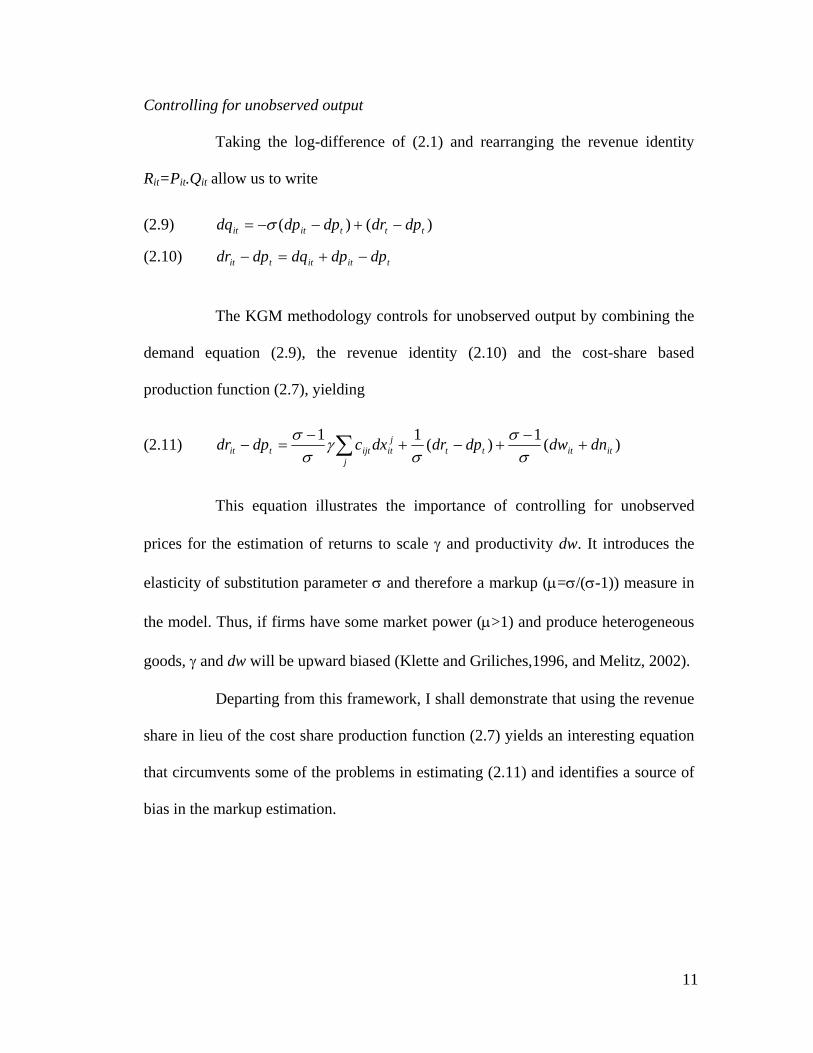
Controlling for unobserved output
Taking the log-difference of (2.1) and rearranging the revenue identity
Rit=Pit.Qit allow us to write
(2.9) )()( tttitit dpdrdpdpdq −+−−= σ
(2.10) titittit dpdpdqdpdr −+=−
The KGM methodology controls for unobserved output by combining the
demand equation (2.9), the revenue identity (2.10) and the cost-share based
production function (2.7), yielding
(2.11) )(1)(11itittt
j
jitijttit dndwdpdrdxcdpdr +
−+−+
−=− ∑ σ
σσ
γσ
σ
This equation illustrates the importance of controlling for unobserved
prices for the estimation of returns to scale γ and productivity dw. It introduces the
elasticity of substitution parameter σ and therefore a markup (µ=σ/(σ-1)) measure in
the model. Thus, if firms have some market power (µ>1) and produce heterogeneous
goods, γ and dw will be upward biased (Klette and Griliches,1996, and Melitz, 2002).
Departing from this framework, I shall demonstrate that using the revenue
share in lieu of the cost share production function (2.7) yields an interesting equation
that circumvents some of the problems in estimating (2.11) and identifies a source of
bias in the markup estimation.
11

Indeed, combining (2.6), instead of (2.7), with (2.9) and (2.10) results in
(2.12) )(1)(11itittt
jitijttit dndwdpdrdxdpdr +
−+−+
−=− ∑ σ
σσ
αµσ
σ
Note that the parameter on the input bundle cancels out, such that:
(2.13) )(1)][(1itittt
j
jitijttit dndwdpdrdxdpdr ++−=−− ∑ µσ
α
The estimation of (2.13) has several advantages over the KGM. First,
since the factor inputs variables appear on the LHS we do not have to worry about
their potential correlation with the productivity term. Therefore, even the OLS
estimator is consistent. Second, as discussed in further detail below, even if there is
still some correlation left between the error term (dwit +dnit) and the remaining
regressor (rt-pt), GMM estimation can be applied with traditional aggregate
instruments, instead of plant-levels ones which are usually difficult to find.
This equation also contains the Solow residual as a particular case. If the
market is in perfect competition, i.e the coefficient on (drt –dpt) is zero, eq. (2.13) is
just the computation rule for the Solow residual. Furthermore, it indicates that the
common finding that productivity is procyclical should be reviewed. It suggests that
the degree of correlation between the TFP growth and the business cycle should at
least be reduced since the residual, dependent variable minus the “fitted” input levels,
represents a measure of the TFP growth plus a term that appears after controlling for
the heterogeneity in prices and that includes an aggregate measure of the industry
output (drt–dpt) as a regressor.
12

Roeger (1995) also develops a strategy to estimate production function
parameters that avoids the necessity of disaggregated instruments4 and that control for
unobserved nominal prices. The basic idea is that both the primal- the one discussed
above- and the dual Solow residual5 contain the same unobservable productivity term
that cancels out if one residual is subtracted from the other. However, his
methodology only works under the hypothesis of constant returns to scale. Omitting
variations in this parameter can cause an upward (downward) bias if returns to scale
are decreasing (increasing) as shown by Basu and Fernald (1997).
Ignoring product differentiation
To estimate markups in a homogenous product industry it suffices to
deflate revenue by a common industry price to proxy quantity, yielding the following
equation:
(2.14) ititj
jitijttit dndwdxdpdr ++=− ∑αµ
By estimating variations of the equation above several plant–level data
studies have either supported competitive or oligopolistic markets with low markups,
usually close to one. For example, Klette (1999) using establishment data from the
manufacturing sector in Norway finds markups ranging from 0.972 to1.088. Although
his estimates are statistically different from one they are incredibly close to this
number. Using panel data of firms from cote d’ivoire Harrison (1993) presents similar
results. She finds supporting evidence of perfect competition for most of the sectors
4 See Konings and Vandenbussche(2004) for a firm level application of Roegers’s methodology. 5 The dual is obtained from the relation between marginal costs, factor inputs and productivity.
13

and low market power for the remaining ones. Below I argue that those results are
driven by a misspecification of the production function.
If we believe that (2.13) is the true data generating process, those
estimates are not so surprising at all. By comparing (2.13) to (2.14) and defining µ) as
a consistent estimator of µ as it appears in (2.14) it easy to show that plim µ) =1. That
is, the markup measure should be one regardless of competitive levels, or at least
evolve around one after considering different sources of biases from standard
econometric techniques.
2.2 Data
The data set analyzed in this chapter was obtained from the census of
Colombian Manufacturing plants, collected by the Departamento Administrativo
Nacional de Estadistica (DANE) and was cleaned by Roberts (1996). It covers all
plants in the manufacturing sector for 1980-1987 period and plants with ten or more
employees after 1982. In this study we consider six different sectors at the three digit
level: 311 (Food Products), 322 (Clothing and Apparel), 381 (Metal Products), 342
(Printing and Publishing), 383 (Electronic Machinery and Equipment) and 384
(Transportation Equipment).
Input data are available for book value of capital, number of employees
and book value of intermediate inputs. Intermediate inputs include material, fuels and
energy that are bundled together to form a unique measure M entering the equations
defined in the last section. The value of gross output is reported and accordingly
14
deflated by a common industry price index. Also, the richness of the data avoids
misspecification problems commonly associated to value-added production functions.
Since there is entry and exit this data set is a dynamic panel characterized
by missing values if a firm did not enter the market in a given year or, alternatively,
has already gone out of business. This dynamic feature of data set causes some
technical difficulties for estimation. A standard way to deal with this problem is to
simply eliminate all firms that do not show up during the whole time period.
Although commonly used, this practice yields a selection bias, which gets worse as
the time period increases. Firms that stay longer are likely to be more productive and
larger. Thus productivity measures are likely to be upward biased.
Note, however that, even with the full sample data set standard estimation
techniques, as OLS, within and Instrumental Variables (IV) estimation, still lead to a
selection bias since they do not take into account information given by input use and
shutdown decision by the firms. Olley and Pakes (1996) –henceforth OP- carefully
modeled these policy variables in a dynamic setup with capital and age fixed in the
short-run and firms choosing the input levels as well as to stay or not in business.
Their estimator addresses two critical problems usually associated to production
functions estimation: the simultaneity and the selection bias. The former is
particularly more severe for plant-level data since consistency of OLS and within
estimates often relies on very restrictive assumptions. Moreover it is usually difficult
to find instruments at the firm level that exhibit enough variation across firms to
explain variability in the regressors.
15

The OP technique nevertheless requires elimination of information on
plants with zero investments. This usually reduces considerably the number of
observations. In contrast, (2.13) presents a particular form that permits the use of
aggregate instruments. Also, the assumptions used to validate OLS estimates are not
as restrictive as commonly argued. And, as far as the selection bias is concerned, I try
to attenuate its magnitude by using the full sample instead of a balanced panel6.
2.3 Estimation
This section presents the markup estimates according to the misspecified
model (2.14) and the true model (2.13) for selected 3-digit industries in the
Colombian manufacturing sector. It should be noted that I randomly selected the
these industries for this study and that I paid no attention to the idiosyncrasies of
neither of them. This is justified here on the basis that the objective in this chapter is
to illustrate the methodological problems of ignoring price heterogeneity rather than
providing a detailed study of the idiosyncrasies of each industry. However, an
application of this methodology to study a particular industry in the Colombia
manufacturing sector would be a natural extension of this work.
6 Olley and Pakes (1996) results do not show much variation between their estimator and the traditional estimation using the full-sample.
16

Misspecified Model Estimation
As discussed above, ignoring price heterogeneity and deflating output by
an industry price index, which amounts to estimating (2.14), yields markup estimates
whose asymptotic value should be one regardless of competitive levels.
However, OLS does not yield consistent estimators of the true value of µ
(µ0=1) in (2.14). Two sources of upward bias can be identified. The former arises
from the potential positive correlation between input choices and productivity levels.
The latter originates from a traditional omitted variable problem caused by the
omission of the term (1/σ)(drt–dpt) in the misspecified equation (2.14). Since the
firm’s input choices are procyclical, i.e., positively correlated with aggregate activity,
it easy to show that this results in an overestimation of the true value v0=1. Results
show nonetheless that OLS are quite informative.
As presented in the first column of Table 2.1 the magnitudes of the
markups are close to one although statistically different from unity for all industries
except for 342. Thus, even though we do not control for the sources of upward biases,
the basic prediction of equation (2.12) that OLS estimates of the markup based on
(2.14) should be approximately one still comes through. If we were to have controlled
for these biases the coefficient would presumably be lower and even less plausible as
markups.
True model estimation
Since the input data are placed on the LHS of true model (2.13), I do not
have to worry about the simultaneity bias. Thus simple OLS regressions can be used
17

without strong assumptions on the co-movements of productivity and input use.
Nevertheless we have to assume that aggregate output, at the industry level, is
uncorrelated with productivity. The validity of this assumption depends upon the
extent that we believe that the productivity term dwit is a pure idiosyncratic shock or
not. If so, it is reasonable to assume that firm-specific shocks do not affect total
output. In a monopolistic competition market with many firms, an increase in the
quantity produced by a firm due to an idiosyncratic productivity improvement has
little effect on the aggregate measure of goods supplied in this market.
Two issues deserve further comments since they cast some doubt on the
OLS estimates of (2.13). First, the argument for using OLS is somewhat weakened if
we consider industry-wide productivity shocks. For instance, a new production
technique developed by a University and publicaly available in a scientific journal
affects every firm equally if we believe that firms have the same capabilities of
absorbing new technologies. Hence, movements in aggregate output are positively
related to movements in the composite shock (firm specific plus industry wide
productivity shock). Also macroeconomic shocks and trade liberalization policies
may equally affect every firm in the industry. Second, despite the fact that our
measure of productivity dw eliminates spurious sources of procyclical movements,
reasonable arguments may support the case for a positive correlation between the TFP
and aggregate fluctuations. One of them relies on the efficiency gains. Firms with
increasing returns to scale may exhibit efficiency gains by expanding supply.
Thus, the validity of OLS estimates relies on the intensity that the sources
of correlation between the regressor (drt –dpt) and the error term are present. If
18

aggregate shocks do not play an important role in the industries in the period
considered here and if firm exhibits relatively low returns to scale there is no reason
to try alternative and also problematic estimation techniques
A common way to control for the presence of industry-wide shocks is to
include time dummies in the econometric model. However, colinearity concerns may
undermine this approach since (2.13) already contains a variable whose only variation
is through time (drt-dpt). Thus, instead of testing for the presence of aggregate shocks
(or high internal returns to scale) I will test the robustness of the OLS results by
comparing them to the GMM estimates of (2.13) and performing a Hausman test to
verify the equivalence between the two techniques. Since the factor input coefficients
do not need to be estimated, the only regressor remaining in this equation is drt-dpt,
which is simply a proxy for the aggregate industry output. Hence, its coefficient (1/σ)
can be estimated by GMM with well-established instruments at the industry level7.
Table 2.1 shows the results for the OLS and GMM estimation of 1/σ. The
instruments set is composed of current and lagged growth rate of international oil
prices deflated by an index of imported goods. The resulting overidentified system
permits testing the validity of the instruments. Hansen (1982) showed that the J
statistic, defined there as the minimized value of the GMM objective function times
the number of observations, converges asymptotically to a chi-square distribution
with degrees of freedom equal to the number of moment restriction minus the number
of regressors under the null hypothesis that the moments are correct.
7 These are classical instruments in the aggregate productivity literature. They are correlated with the aggregate activity but not with productivity.
19

Note that a significant 1/σ estimate implies imperfect competition (σ is
finite) whereas a insignificant estimate supports the alternative hypothesis of perfect
competition .The implied markups (σ/σ-1) reported in the Table 2.1 show firms with
high market power, considerably above one in most of the sectors contrasting with the
markup estimates of (2.14) that report estimates close to one. This is a strong result.
Controlling for price heterogeneity yields markups much higher than the ones
implied by the misspecified model (2.14), which already contain upward biases.
The OLS estimates proved to be robust to the alternative estimation
technique since GMM estimates show similar point estimates for 1/σ. However due
to larger standard errors, data for industry 381 cannot reject the hypothesis of
competitive market. The model also passes the overidentification test for all industries
but one (383) confirming the finding that a negative 1/σ is inconsistent with the
assumptions imposed so far. A negative σ implies an upward sloping demand
schedule which is clearly inconsistent with the underlying monopolistic competition
demand function. The Hausman test confirms that OLS and GMM are statistically
equivalent estimation procedures. This result is consistent with the hypothesis that the
aggregate industry output is not significantly correlated with the error term.
2.4 Robustness checks
Measurement error
In many cases, the data collected for the factor inputs reflect installed
capacity, not the real level of factor utilization. In a recession, managers would rather
20

reduce the utilization level of the existing machines than sell some of them. Similarly,
they would rather reduce labor hours than lay off workers (labor hoard). Thus, using
the reported data directly in the production function estimation is potentially
misleading and yields a classical measurement error problem.
Rewriting (2.13) with an additional term dg, representing a measurement
error in the input levels, and denoting Y* as the LHS of (2.13) imply
(2.15) dwdgdpdrY tt }1{)(* 21 σσββ −
++−=
Now, defining as the OLS estimator of 1̂β 1β (β1=1/σ), and ignoring dg in
the OLS regression of the equation above yields the following asymptotic result
(2.16) 111 )(),cov(ˆlim βββ
tt
tt
dpdrVdpdrdg
p−−
+=
Thus, if changes in factor utilization are positively correlated with changes
in total industry output overestimates the parameter of interest 1/σ. Therefore β1̂β 1
may be capturing variations of factor utilization in addition to the measure of demand
elasticity. In the most extreme case, a significant may still show up even if
markets are perfectly competitive. Thus, not controlling for the measurement error
may be misleading us to conclude that markups are well above one and that markets
are in imperfect competition.
1̂β
To approximate the unmeasured term I use total wages expenditure per
employee. The choice of this proxy is justified by the assumption that workers are
rewarded based on variations in effort levels and that capital and labor utilization
21

rates are proportional 8. Results in Table 2.2 show that magnitudes do not change
significantly once the measurement error proxy is introduced in the model. This result
should be taken with caution though, since wages are expected to be endogenous.
Externalities
Theoretical models in macroeconomics have emphasized the importance
of external returns to predict and explain growth and business cycles trajectories. In
the growth literature for example the presence of externalities measured by aggregate
output or total employment help to explain why countries may exhibit long-run
growth even in the presence of constant or decreasing internal returns to scale. It is
based on the premise that human capital is a public good and therefore individual
firms should benefit from its aggregate level9. Also, Howitt (1985) considers the
reduction in the costs of transactions as the level of activity increases. Below a brief
summary of the findings in the empirical literature is presented.
Caballero and Lyons (1990) used European data at the 3-digit level (ISIC)
to measure economy-wide externalities. They approximated the externality effect by
aggregated output and found strong evidence of external returns. Following the same
framework, but using highly disaggregated data, Krizan (1998) and Lindsdtrom
(1999) found similar results. On the other hand Basu and Fernald (1995) using U.S
manufacturing data found no evidence of gross output related externalities. They
8 See Lindstrom (1997) for further details. Also I am implicitly assuming that materials are costlessly adjusted and therefore do not preset measurement errors. 9 See Lucas(1988).
22

argued that value-added output data fail to account properly for the intermediate
inputs leading to spurious externalities measures due to misspecification.
In this section I consider the consequences of neglecting external effects in
(2.13) on the markup estimates. I begin by defining the externality proxy as lagged
aggregate activity (rt-1-pt-1). More precisely it is assumed that individual firms should
benefit from past levels of industry–wide production10. However due to colinearity
problems only one lag is considered in the estimation procedure. This specification is
motivated by the idea that external effects do not have an immediate impact on firms’
efficiency. Instead they take one period to be effective. In this sense, the external
effect could be capturing learning-by-doing and human capital spillovers if we are
willing to assume that lagged aggregate production is a reasonable approximation to
both variables.
In order to check the robustness of the markup measures to the inclusion
of the externality effect in the revenue production function the following equation is
estimated
(2.17) dwdpdrdpdrY tttt }1{)()(* 1121 σσββ −
+−+−= −−
where all the variables are defined as in (2.16). Similarly to the measurement error
case neglecting (rt-1–pt-1) yields an upward bias in the estimation of 1/σ since the
aggregate deflated revenues series (rt–pt) are expected to be serially correlated.
Indeed, the results shown in the last column of Table 2.2 support the claim
of an upward bias. Except for 322 and 342, the 1/σ estimates are smaller than those
10 Cooper and Johri (1997) used lagged aggregate activity to study dynamic complementarities.
23

obtained by the OLS estimation of (2.13). However the bias is not severe enough to
change the significance of the estimates or to affect their magnitude considerably.
2.5 Fixed Capital
Although the econometric model represented by (2.13) is consistent with
the results presented in the previous sections it relies heavily on the assumption that
firms choose their inputs levels in a sequence of static problems and that factor
markets are competitive. These assumptions are certainly more problematic for
capital. In order to decide how much to invest in a given period, agents take into
account past levels of capital. Indeed, dynamic models of firm’s decision problems
have emphasized capital as a state variable, which enters as a parameter in the choice
of investment, employment, and materials levels.
Hence, those assumptions, crucial to derive (2.13), may potentially yield
misleading conclusions. Yet, as I shall argue below, the basic predictions of last
section remain and the data also supports the same claims as before when weaker
assumptions on the capital input decision are taken into consideration.
Model
Now, I assume that capital is fixed in the short-run. Thus, (2.5) no longer
holds for this input. Hence, (2.13) is no longer valid. Obviously, its main virtues, a
better argument for OLS and the use of industry-level instruments cannot be claimed
in this new set up.
24

With fixed capital and assuming that (2.5) holds for the remaining inputs
the log differentiated production function can be written as
(2.18) iij
ij
iijii dndwdxdxdxdq ++−+= ∑= 3,2
11 )(αµγ
This equation, (2.9) and (2.10) form a system that yields the following
revenue production function
(2.19) ititttitj
itj
itijttit dndwdpdrdxdxdxdpdr ++−+−
=−−− ∑= µσ
γσ
σα 1][1)(1)( 1
3,2
1
Specification (2.18) is the most commonly used in this literature. Not only
it relaxes the strong assumptions on capital but it also permits the estimation of
internal returns as well as markups. However the assumption of homogenous product
still leads to misleading estimates of markups.
Using firm’s revenue deflated by a common industry price to control for
the unobserved firm-specific output results in the following equation:
(2.20) itititj
itijtmittit dndwdxdxdxdpdr ++−+=− ∑ )( 11 αµγ
Again, if we believe that (2.9) is the true model it becomes clear that µ) ,
now the estimator of µ as it appears in (2.20), converges in probability to one
regardless of competition levels. Note that (2.19) is similar to (2.13). The only
fundamental difference is that coefficient on capital (dx1) cannot be placed on the
LHS of the estimating equation and therefore aggregate instruments are no longer
sufficient to ensure consistency. Furthermore, the arguments in favor of OLS are
somewhat weakened since dx1 appears as a regressor in (2.19) and is expected to be
correlated with the error term.
25

In the absence of good disaggregate instruments researchers started
searching for alternative methods to deal with the simultaneity problem. Leading this
recent literature, the OP method proposes an innovative technique that avoids the
difficult task of searching for instruments. This method can be briefly summarized as
follows. Using the information that investment levels are a deterministic function of
productivity levels and by inverting this relationship, it is possible to uncover the
unobservable productivity term as a non-parametric function of investment and the
state variable capital. In this way, the only unobservable error term left in the
estimation is not expected to be correlated with the regressors.
Another way to deal with this problem was developed by Levinhson and
Petrin (2000)-LP hereafter. They argue that investment may only respond to the “non-
forecastable” part of the productivity term since the capital input may have already
adjusted to its “forecastable” part. Therefore some correlation would still remain
between the regressors and the error term.
By using intermediate inputs to proxy the productivity term they are able
to develop a simpler methodology that improves on the OP methodology since
intermediate inputs respond to the whole productivity shock. It also avoids a major
drawback of the OP method, which is the necessity to drop information on industries
that report zero investment in a given period.
The availability of intermediate input in our data set and the arguments
discussed above make the LP our natural choice for estimating equation (2.19). It is
worth pointing out however two limitations concerning the LP method. First, it does
not control for the selection bias. That is, unlike OP, it does not use information on
26

firms shut down decision rule in the estimation process. Second, it assumes
competitive and homogeneous product markets to validate the use of the intermediate
output as proxy for the unobservable term.
While the effects of former limitation can be partially attenuated by the
use of the full-sample instead of a balanced panel, the effects of the latter requires a
more careful look into the technique itself, for our model assumes a differentiated
product market, not a homogeneous one.
The basic result that supports LP is the monotonic relation between
productivity and the optimal intermediate input level. In a competitive framework it is
straightforward to prove that. With fixed output and input prices an increase in
productivity implies a higher intermediate input marginal product at the existing input
levels. Therefore firms will decide to produce more output so that marginal product
falls back to equal the intermediate input price. Therefore as output goes up demand
for inputs also increases.
In an oligopolistic market this monotonic property may not hold anymore.
The marginal product still follows the same qualitative movements as before, but now
firms realize that prices decrease as output goes up. Thus, the net effect of a supply
expansion will ultimately depend on the elasticity of demand. It is possible to set up a
scenario where one firm facing higher demand elasticity actually reduces output
whereas another firm facing less responsive prices increases production levels. In a
monopolistic competitive environment, however, the proof of the monotonic
condition is very similar to the one presented in Levinsohn and Petrin (2000) and,
therefore, will be omitted here.
27
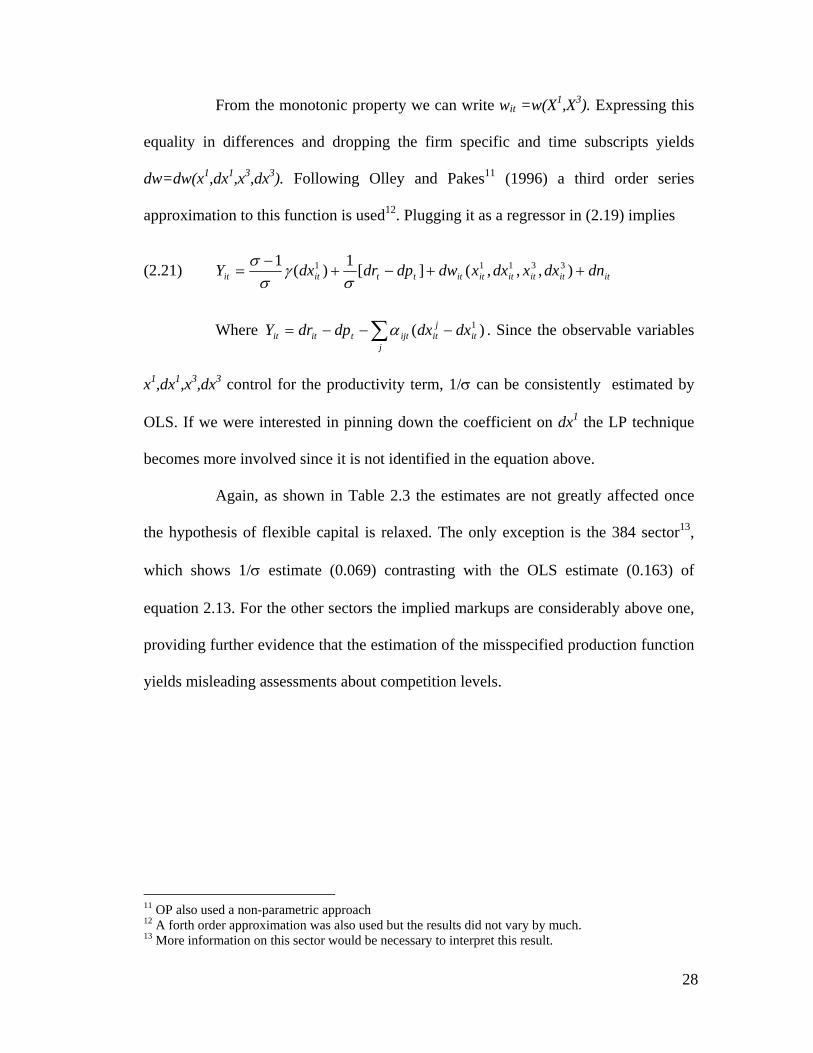
From the monotonic property we can write wit =w(X1,X3). Expressing this
equality in differences and dropping the firm specific and time subscripts yields
dw=dw(x1,dx1,x3,dx3). Following Olley and Pakes11 (1996) a third order series
approximation to this function is used12. Plugging it as a regressor in (2.19) implies
(2.21) ititititititttitit dndxxdxxdwdpdrdxY ++−+−
= ),,,(][1)(1 33111
σγ
σσ
Where ∑ −−−=
jit
jitijttitit dxdxdpdrY )( 1α . Since the observable variables
x1,dx1,x3,dx3 control for the productivity term, 1/σ can be consistently estimated by
OLS. If we were interested in pinning down the coefficient on dx1 the LP technique
becomes more involved since it is not identified in the equation above.
Again, as shown in Table 2.3 the estimates are not greatly affected once
the hypothesis of flexible capital is relaxed. The only exception is the 384 sector13,
which shows 1/σ estimate (0.069) contrasting with the OLS estimate (0.163) of
equation 2.13. For the other sectors the implied markups are considerably above one,
providing further evidence that the estimation of the misspecified production function
yields misleading assessments about competition levels.
11 OP also used a non-parametric approach 12 A forth order approximation was also used but the results did not vary by much. 13 More information on this sector would be necessary to interpret this result.
28

2.6 Final Remarks
This chapter shows that neglecting output price heterogeneity in plant or
firm level studies can be misleading, yielding spurious markup estimates. Assuming a
differentiated product market, a competitive factor market and strong assumptions on
firms’ input level decisions yields an econometric model that demonstrates that a
misspecified version of Hall’s equation implies markups equal to one regardless of
the market environment. Furthermore, this model avoids the search for good
disaggregated instruments, usually difficult to find, and can be consistently estimated
by GMM and even OLS. These consistent estimates, in turn, show markups much
higher than one.
I also perform robustness checks by controlling for alternative
explanations that could be driving our finding of a significant coefficient on the
output aggregate measure (measurement errors and externalities). Robust estimates of
1/σ are found. Its statistical significance and magnitude present very little change
compared to the previous estimates.
In the latter part of the chapter I recognize that those nice features, the use
of aggregate instruments and the validation of the OLS estimation, come at the cost of
imposing a restrictive assumptions on the model. Yet, relaxing the most disputable
assumption imposed in the first part of the chapter (flexible capital) does not change
the results significantly.
29

References
Aitken, B. and Harrison, A. (1999), “Do Domestic Firms Benefit from Foreign Direct Investment? Evidence from Panel Data,” American Economic Review, 89(3), pp. 605-618.
Basu, S. and Fernald, J. (1997). “Returns to Scale in U.S production: Estimates and
Implications” Journal of Political Economy 105,249-283. Bartelsman, J., Caballero, R. (1991), “ Short and Long Run externalities”, NBER
Working Paper No. 3810. Caballero, R. and Lyons, R. .(1991). “Internal Versus External Economies in
European Industry.” European Economic Review 34,805-26. Cooper, R. and Johri, A. (1997) “Dynamic Complementarities: A Quantitative
Analysis” Journal of Monetary Economics 40, pp. 97-119. Griliches, Z. (1957), “ Specification Bias in Estimates of Production Functions”,
Journal of Farm Economics, 39, pp 8-20. Griliches, Z. and Mairesse, J. (1995) “Production Functions: the Search for
Identification”, NBER Working Paper No. 5067. Hall, R.(1988). “The Relation Between Price and Marginal Cost in U.S. Industry”
Journal of Political Economy 96. Hall, R. (1990). “ Invariance Properties of Solow’s Productivity Residual”, In P.
Diamond (ed.), Growth, Productivity, Unemployment, MIT Press, Cambridge, MA.
Harrison, A. (1994) “Productivity, Imperfect Competition and Trade Reform: Theory and Evidence”. Journal of International Economics 36, 53-73.
Klette, T.J. (1999): “Market Power, Scale Economies and Productivity: Estimates
from a Panel of Establishment Data” Journal of Industrial Economics, 47, pp. 451-76.
Klette, T. and Griliches, Z. (1996), “The Inconsistency of Common Scale Estimators
When Output Prices Are Unobserved and Endogenous,” Journal of Applied Econometrics, 11(4), pp. 343-61.
Krizan, C. J.(1995). “External Economies of Scale In Chile, Mexico and Morrocco:
Evidence from Plant-level Data”. Georgetown University, Washington, D.C.
30

31
Konings and Vandenbussche(2004). “Antidumping Protection and Markups of Domestic firms: Evidence from Firm-Level data”. LICOS Discussion Paper No.141.
Levinsohn, J.(1993). “Testing the Imports-as-Market-Discipline Hypothesis”. Journal
of International Economics 35,1-22. Levinsohn, J. and Petrin, A. (2000), “Estimating Production Functions Using Inputs
to Control for Unobservables” NBER Working Paper No. 7819. Lindstrom, T. (1997).“External Economies at the Firm Level: Evidence from Swedish
Manufacturing” Mimeo. Lucas, R. (1988) “ On the mechanics of economic development”. Journal of
Monetary Economics, 22, pp. 3-42. Melitz M. J.(2000) “Estimating Firm-Level Productivity in Differentiated Product
Industries”. Mimeo. Mundlak, Y. and Hoch, I. (1965) “ Consequances of alternative Specifications of
Cobb-Douglas production functions”, Econometrica,33, pp. 814-828.
Olley, S. and Pakes, A. (1996), “The Dynamics of Productivity in the Telecommunications Equipment Industry,” Econometrica, 64(6), pp. 1263-1297.
Roberts, Mark (1996). “Colombia, 1977-85: Producer Turnover,Margins, and Trade
Exposure”. In Mark Roberts and James Tybout, editors, Industrial Evolution in Developing countries. New York: Oxford University Press.
Roeger, W. (1995) “Can imperfect Competition Explain the Difference between
Primal and Dual Productivity Measures? Estimates from US Manufacturing”. Journal of Political Economy, 103(21).
Tirole, J. (1988), The Theory of Industrial Organization, MIT Press, Cambridge, MA.
Tybout, J. (forthcoming) “Plant and Firm-level evidence on the ‘New’ Trade
Theories” in James Harrigan (ed.) Handbook of International Trade, Oxford: Basil-Blackwell.

Table 2.1: Parameters Estimates 14
Method OLS
OLS
GMM15 Hausman test16
Specification Equation (2.14 ) Equation (2.13 ) Equation (2.13 ) v estimates 1/σ Estimates Implied
markups 1/σ Estimates Jstatistic Implied
markups
311 0.975(0.0078)
0.380 (0.0277)
1.61
0.415 (0.1407)
1.723 1.71 0.064
322 1.065(0.01060)
0.392 (0.0325)
1.63
0.454 (0.1402)
0.889
1.81 0.203
381
1.052 (0.0124)
0.330 (0.0374)
1.49
0.300 (0.2202)
0.606 1.43
0.018
342 0.964(0.0204)
0.413 (0.0416)
1.72 0.447(0.1620)
3.871
1.78 0.048
383
1.036 (0.0212)
-0.244 (0.0681)
inconsistent -0.266(0.2925)
7.469 inconsistent -
384
1.065 (0.0205)
0.163 (0.0328)
1.20
0.220 (0.1285)
0.615 1.29
0.206
14 Standard errors in parentheses. 15 GMM is performed with the following instruments: current and lagged growth of the international oil price and a constant.. χ(1)=5.02 is the critical value at 5% significance level. 16 This column presnts the results of a Hausman Test between OLS and GMM estimation of (1.9). χ(1)=5.02 is the critical value at 5% siginificance level.
32

Table 2.2: Robustness Checks
Method OLS
OLS
Specification Equation (2.15 ) Equation (2.17 ) β1 Estimates β1 estimates
311
0.317(0.0284)
0.369 (0.0373)
322 0.148(0.0337)
0.583 (0.0412)
381
0.385 (0.0373)
0.334 (0.0401)
342 0.416(0.0415)
0.449 (0.0407)
383
-0.297 (0.0694)
-0.307 (0.0691)
384
0.185 (0.0328)
0.157 (0.0341)
33

Table 2.3: Fixed Capital
Method OLS
OLS
Specification Equation(2.21 ) 1/σ Estimates Implied Markups
311
0.417(0.2154)
1.71
322 0.434(0.1216)
1.77
381
0.208 (0.1944)
1.27
342 0.443(0.0412)
1.79
383
-0.2116 (0.3510)
-
384
0.0699 (0.5761)
1.08
34

Chapter 3
Uncovering Marginal Cost and Quality from Revenue and Cost Data
With assumptions on a discrete-choice demand system, technology,
Katayma, Lu and Tybout (2003), KLT henceforth, develop a methodology to uncover
marginal costs, quality, prices and quantities from plant-level data that report only
revenue and cost data. Once these variables are determined it is possible to perform
policy analysis and counterfactual experiments as discussed in the next chapter.
Using data from the Colombian beer industry, originally containing only
plant-level information on revenue and total costs from 1977 to 1990, I shall
demonstrate how to extend the KLT framework by including the extra information
provided by aggregate data. Although it may be difficult to obtain detailed data on
quantities at the plant level, the same is not true for aggregate variables. For instance,
in the beverage sector, the amount of beer, in liters, consumed in a given year is
widely available for many countries. Aggregate quantities also carry information on
demand parameters and therefore may help in the estimation process, especially in
small data sets. I consider two different hypotheses on the nature of this aggregate
measure. The first one assumes that this information is noisy, while the second
assumes that this information is deterministic and therefore error free. Each
assumption yields a different estimation strategy with potentially different parameter
estimates.
35

This chapter is organized as follows. Section 1 describes the traditional
approaches to estimating discrete-choice based demands. The next section provides
details of data set to be analyzed. The following section shows how to incorporate the
aggregate information into the model. And finally, the last section discusses the
results.
3.1 Traditional approaches
In this section, I shall describe the discrete-choice model commonly used
in the literature and the different econometric strategies to estimate its parameters.
Consumers rank products according to their characteristics and prices.
There are N+1 choices in the market, N inside goods and one outside good. Consumer
i chooses among those goods, given prices pj, observed characteristic xj, quality ξj and
unobserved idiosyncratic preferences εij , according to the following equation
ijjijijij hphxu εξθβθβ ++−= );();( 2211
where );(1 dih θβ is a function of a vector demographic variables hi, like
income , age, and marital status and 1θ is a vector of parameters defining that
function. The coefficient for price, );( 22 θβ ih , is defined similarly.
Assuming that εij has a Type I Extreme Value distribution, the probability
of individual i choosing good j takes the familiar logit form
(3.1) ∑ +−
+−=
kjikik
jijiji hphx
hphxhjp
));();(exp());();(exp(
)/(2211
2211
ξθβθβξθβθβ
36

If the econometrician observes prices, individuals’ choices and their
characteristics, the vector of parameters can be estimated by setting up the maximum
likelihood profile of all the observed consumer choices. Goldberg (1995) and
Trajtenberg (1990) are two examples of this approach. The former author observes
the new car choices of a random sample of consumers in the U.S from the Consumer
Expediture Survey, whereas the latter author collected data on purchases of CT
scanners1.
Suppose now that consumer-level data is not available, the econometrician
observes only prices, market shares, and characteristics. Then, the estimation
procedure has to be changed, since it is no longer possible to construct the maximum
likelihood profile. Instead, some aggregation argument has to be invoked. Indeed,
taking the expected value with respect to consumer attributes h yields the market
share implied by the model )]/([ hjpEs jj = which in extensive form is simply
(3.2) ∫∑ +−
+−= )(
));();(exp());();(exp(
),,,(2211
2211 hdFhphx
hphxpxs
kjikik
jijijj ξθβθβ
ξθβθβξθ
A regression equation can now be written by matching observed market
share of product j ( js ) with the one implied by the model, which gives
(3.3) ),,,( ξθpxss jj =
Firms take into account the unobservables (ξ) when setting its prices.
Thus, the endogeneity of prices requires the use of instrumental variables. However,
since the unobservables enter the regressions equation non-linearly some simulation
37
1 Actually, these authors use a variation of the logit model known as the nested logit model, which I shall discuss later in this chapter.

method has to be applied. Shortly, it involves solving for the ξj’s given data and the
parameters to construct moment restrictions conditional on available instruments (for
further details see Berry, Levinshon, and Pakes,1995).
When setting prices, firms take into account demand and cost
determinants. Therefore, the pricing decision also contains information on consumer
preferences such that efficiency can be improved by incorporating it in the estimation
procedure. And, as it shall be demonstrated in a later chapter, it also allows for the
simulation of different economic environments.
First, assume that each firm f produces a subset Ff of the goods sold in this
market and maximizes the sum of profits given by
(3.4) ∑∈
−=ΠfFj
jjjf sMmcp .).(
where M is the total market size and mcj is the marginal cost of producing
brand j. Then, it can be shown that the price pj of any product j produced by firm f
must satisfy the following equation
(3.5) 0)( =∂∂
−+ ∑∈ fFr j
rrrj p
smcps
Note that (3.5) is flexible enough to accommodate different market
structures. The first structure is the single firm product, in which the firm can only
control the price of its unique brand. The second is the multi-product firm, in which
the firm internalizes the price decision of all of its brands. I shall discuss these
different market structures in a separate section.
38

In turn, let marginal cost be modeled as
jjj wmc ψγ +=
where wj is a vector of cost characteristics and jψ is an unobserved cost
component. Similarly to the demand side unobservable, given ),,,,,( γξθ wpx one can
solve for the vector ψ from the quasi-supply relation (3.5) and set up the moment
conditions based on appropriate instruments. All the parameters of the model can then
be estimated through GMM using the demand and supply side moments. KLT goes a
little further by devising a methodology to estimate the demand parameters without
directly observed market-level data (prices and market shares).
3.2 Data
The data set consists of an unbalanced panel of plants in the beer industry,
with more than 10 employees, covering the period from 1977 to 1990. Originally
these data were gathered by the Colombia’s Departamento Nacional de Estadistica
(DANE) and have been cleaned as described in Roberts (1996). The revenue series
are constructed as the total sale revenue divided by a general wholesale price deflator.
The total variable costs are defined as the sum of payments to labor, intermediate
input purchases and energy purchases. Since some of the cost is incurred in the export
activity one has to scale it by the ratio of total domestic sales to total sales and deflate
the result by the same wholesale price deflator mentioned before.
From an additional source (UN database) I obtain the quantity of beer (in
hectoliters) produced in the country for the same sample period. Ideally, one would
39

want to have data on the quantity of beer consumed in the country. However, the data
in hand is not so restrictive since there is very little export activity in this sector
I also use auxiliary data to uncover the price of the imported good (p0t) 2 as
well as its imported quantity in hectoliters (q0t). In a separate publication DANE also
reports the net weight (in kilos) and the monetary value of imports (in pesos).
Assuming that beer has the same density as water (1kg per liter) it easy to transform
the net weight in kilos to volume of imported beer in hectoliters (q0t). Then, p0t
follows from the ratio of the peso value of imports to q0t.
3.3 Model
In this section I shall lay out the model used in this investigation. For
expositional purposes I assume first that market-level data on prices and quantities are
available. Then, I shall demonstrate, how to estimate the model with limited data
(only revenue and cost data) according to the methodology developed by KLT.
Assume now that products are divided into nests, g=0,1. The first nest
contains only the outside good (imported variety) while the second collects all the
inside goods (domestic varieties). For product j belonging to nest g define utility as
ijigjjij pu εσςαξ )1( −++−= for j=0,1,..,N
The first random term on the RHS ( igς ) is a common shock to all products
in nest g and its distribution depends on the parameter σ ( 10 <≤ σ ). As σ
approaches zero the within correlation of utilities within each nest decreases.
2 This as composite good that bundles together all the different imported varieties.
40
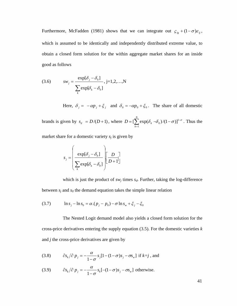
Furthermore, McFadden (1981) shows that we can integrate out ijig εσς )1( −+ ,
which is assumed to be identically and independently distributed extreme value, to
obtain a closed form solution for the within aggregate market shares for an inside
good as follows
(3.6) ]exp[
]exp[
0
0
δδ
δδ
−
−=
∑ kk
jjsw , j=1,2,…,N
Here, =jδ jjp ξα +− and 000 ξαδ +−= p . The share of all domestic
brands is given by )1/( += DDsd , where . Thus the
market share for a domestic variety s
σσδδ −
=
−−= ∑ 10
1)]1/()exp([
N
kkD
j is given by
⎥⎦⎤
⎢⎣⎡
+⎟⎟⎟⎟
⎠
⎞
⎜⎜⎜⎜
⎝
⎛
−
−=
∑ 1.
]exp[
]exp[
0
0
DDs
kk
jj
δδ
δδ
which is just the product of swj times sd. Further, taking the log-difference
between sj and s0 the demand equation takes the simple linear relation
(3.7) 000 ln).(lnln ξξσα −+−−=− jwjj sppss
The Nested Logit demand model also yields a closed form solution for the
cross-price derivatives entering the supply equation (3.5). For the domestic varieties k
and j the cross-price derivatives are given by
(3.8) ])1(1[1 wjjjk sssps σσ
σα
−−−−
−=∂∂ if k=j , and
(3.9) ])1([1 wjkjk sssps σσ
σα
−−−−
−=∂∂ otherwise.
41

If prices and quantities were available the model above could be estimated
using the methodologies described in section 3.1. Indeed, notice that, under some
rearrangements, (3.7) is a closed form version of (3.3) that can be solved, up the
model parameters, for the unobservable term 0ξξ −j . Also, the marginal cost
unobservable can be uncovered by substituting equations (3.8) and (3.9) into firms’
FOC (3.5). Then, these unobservables can be combined with appropriate instruments
to estimate the parameters through GMM.
Obviously, in the absence of market level data (prices and quantities) this
strategy is unfeasible. However, KLT show that commonly available information on
revenue and total costs along with some assumption on the technology can be used to
uncover relevant variables and estimate the model.
Using the fact that Rj=pj.qj, TCj=mcj.qj, and sj=qj/(Q+Q0) where Rj ,TCj, Q
and Q0 are revenue, total variable cost3, total output produced by domestic firms and
total imported quantity respectively, it is easy to demonstrate that these two identities
together with the F.O.C (3.5) can be solved for quantity as a function of data
(Rj,TCj,Q0t) and the demand parameters (α,σ)
Similarly, from the same system of equations one can retrieve
mcjt=mcjt(α,σ,Rjt ,TCjt, Qt ,Q0t), pjt= pjt(α,σ,Rjt ,TCjt, Qt ,Q0t) . Assume temporarily
that Qt is not observed. Thus, from ∑ =N
tttjtjtj QQQTCRq ),,,,,( 0σα , one is able to
solve for Qt=Qt(α,σ,Rjt ,TCjt,Q0t). Then, using prices and market shares, relative
quality, defined as tjtjta 0ξξ −= , can be determined from the demand system. To
3 TCj=mcj.qj as long as marginal costs are flat.
42

summarize, for a given set (α,σ,Rjt ,TCjt,Q0t), the KLT algorithm shows how to obtain
firm level prices, marginal costs, relative quality and quantities as well as aggregate
output (Qt). For more details see appendix A, which is a generalization4 of the
original transformation algorithm found in KLT.
Moreover, dynamics is introduced into the model through the assumption
that relative quality and marginal cost follow a VAR process given by
ajtjt
cjtjt tmcaba εβϕϕ ++++=+ 011
cjtjt
ajtjt tamcbmc εφλλ ++++= −− 1102
Estimation strategy
From the demand system, the price setting game and the VAR one is able
to uncover demand and supply side “errors”, represented respectively by and .
At this point the model seems awfully close to the BLP (Berry, Levinsohn and
Pakes,1995) methodology where similar error terms are combined with exogenous
product characteristics to form the identifying moment conditions. Here, however,
these data are not available. Note that not even prices or quantities are observed; they
are themselves functions of data and demand parameters to be estimated within the
model. The model is therefore not identified such that traditional econometric
technique like GMM and ML do not apply.
cjtε a
jtε
To identify it more structure has to be imposed on the parameters. This is
achieved by assuming a prior knowledge of the parameters distribution and using the
43
4 The original transformation algorithm had to be modified to accommodate multi-plant firms.

data set and the structure imposed by the model to update this prior according to the
Bayes rule
)().;();( θθθ pDLDp ∝
The LHS is the posterior probability updated by the data D, and the RHS
is the product of the likelihood function of the data times the prior distribution of the
parameters. However, only in special cases, the posterior distribution has a closed
form from which one can make inference either by sampling from it or by consulting
easily available tables. Fortunately, Monte Carlo techniques have been developed to
deal with such problem. Shortly, it relies on ergodic theory to guarantee that a
computable statistic converges to the true posterior distribution. Then, once
convergence has been attained, one can sample from this statistic and make inference.
3.4 Aggregate information
Aggregate quantities also carry information on demand parameters and
therefore may help in the estimation process, especially in small data sets. Below I
discuss two different assumptions on the properties of this aggregate measure. The
first one amounts to just appending the KLT econometric approach described above,
while the second yields a completely different estimation approach.
Assumption 1: Aggregate information is noisy.
Assume now that the amount of beer consumed in a given year is observed
up to a measurement error. Note that the model implies an aggregate quantity given
44

some parameters and data. One can then ask the model to match this observed
quantity according to
(3.10) tobstjtjtt wQQTCRQ −=),,,,( 0σα
where wt is assumed to be a serially uncorrelated and normally distributed
mean zero error term which is independent of the VAR error terms. To include this
new “moment” in the estimation it suffices to incorporate the likelihood of in the
likelihood function
tobsQ
);( θjtDL .
Assumption 2: Aggregate information is not noisy and σ=0
From this assumption one can conclude that the quantity implied by the
model matches exactly its empirical counterpart and that the discrete choice model is
the simple logit form instead of its nested version (σ=0). Then
(3.11) obstjtjttt QQTCRQ =),,,( 0α
All data in this equation are observed which implies that αt can be
determined for each time period t. This approach has two limitations though. Firstly,
the simple logit model (σ=0) places very restrictive assumptions on consumer
preferences such that cross-price elasticities have somewhat undesirable properties.
Secondly, it requires a very reliable source for the total quantity since measurement
error is not allowed.
45
Given these drawbacks, a legitimate question may arise. Why bother
making these restrictions on the model (assumption2)? The reason is that the
Bayesian technique proved to be a little cumbersome to implement computationally

and many government agencies and students are somewhat reluctant to adopt the
Bayesian approach, especially one that requires Monte Carlo simulation. This
technique also requires the imposition of priors on the parameters distribution, which
even some leading researches are reluctant to do.
In contrast, assumption 2 allows for the estimation, at least of the VAR
parameters, through well-established econometric techniques, like maximum
Likelihood.
The algorithm goes as follows.
Step 1: Solve for αt from (3.11).
Note that once αt is pinned down mcj(αt,Rj,TCj,Q0) and aj=aj(αt,Rj,TCj,Q0)
become data and the VAR can be estimated according to standard ML.
Step 2: Estimate the VAR parameters from the maximization of );( θDL
3.5 Market idiosyncrasies and Results
While it is common for data sets to report plant-level revenue and cost
data, they do not usually contain information on plant ownership. This is important
for estimation since each ownership arrangement implies a different supply function
and therefore, given (α,σ,Rjt ,TCjt,Q0t), different values for the unobserved variables
(price , quantities, marginal cost and qualities). In the Colombian beer sector,
however, ownership identification does not pose a problem since one Company
(Bavaria S.A) controlled the whole non-imported beer market during the sample
period studied here.
46

Indeed, after an aggressive horizontal merger strategy, Bavaria became a
monopoly in the beer production by acquiring all of its rivals (Cerveceria Aguila,
Cerveceria Union and Cerveceria Andina and other smaller producers) in the beer
business by the early seventies. Its monopoly went unchallenged until 1995 when
Cerveceria Leona entered the beer market as retaliation for the Bavaria entry in the
soft drinks business, which was dominated by Leona’s parent company. Since the
data sample period ranges from 1977 to 1990 all the estimations presented below
assume that a single firm owns all plants.
Three different models are implemented: the Nested Logit model and the
simple logit model, both based on bayesian techniques and assumption 1 (NLB and
SLB henceforth) and the simple logit model, implemented according to assumption 2,
which requires a partial calibration approach (PC from now on). The first two variants
are also estimated without the information on the aggregate quantity, which amounts
to the original version of the KLT model (for details on the estimation technique see
Appendix B).
The Bayesian estimates for the demand parameters seem to be relatively
sensitive to the inclusion of the aggregate moment5. For the SLB model, the disutility
of price α goes from 3.115 to 3.294 (see first two columns of Table 3.1). On the other
hand, the same is not true for the VAR estimates, which do not show significant
changes. The NLB version follows the same pattern, little sensitivity for the VAR
parameters estimates and a noticeable difference for the demand parameters. This
should not come as a surprise, since the new moment incorporated into the model
47
5 Figures 3.1 to 3.3 show the monte carlo simulation for the demand parameters calculated with the aggregate moment for both the SLB and NLB models.

bears only on the demand parameters. Finally, notice that in both the SLB and the
NLB specification there is a precision gain (smaller standard errors) in introducing
the extra information into the econometric models. This is true for all the demand
parameters estimates and for most VAR estimates.
Table 3.1: Parameters Estimates
SLB NLB PC
W/ agg. Moment wo/
agg. moment
w/ agg. moment
wo/ agg. moment
α
3.115 (0.215)
3.294 (0.234)
2.738 (0.193)
3.122 (0.828)
3.046
σ
0.941 (0.010)
0.960 (0.015)
Quality equation (VAR) Const.
15.806 (2.459)
14.867 (2.384)
20.287 (4.495)
19.232 (4.934)
22.333 (4.830)
Lagged Quality
0.333 (0.112)
0.439 (0.109)
0.026 (0.068)
0.022 (0.069)
0.001 (0.063)
Lagged Marg.Cost
0.060 (0.055)
0.036 (0.060)
1.279 (0.289)
1.292 (0.295)
1.441 (0.308)
Trend
-0.143 (0.023)
-0.146 (0.025)
-0.204 (0.052)
-0.191 (0.058)
-0.223 (0.055)
Cost equation (VAR) Const.
6.146 (2.874)
5.874 (2.593)
-0.542 (1.249)
0.669 (1.265)
0.284 (0.839)
Lagged Quality
-0.357 (0.111)
-0.285 (0.100)
-0.042 (0.018)
-0.041 (0.018)
-0.0453 (0.0123)
Lagged Marg.Cost
0.690 (0.063)
0.659 (0.065)
0.752 (0.075)
0.745 (0.075)
0.786 (0.055)
Trend
-0.062 (0.027)
-0.061 (0.026)
0.005 (0.014)
0.006 (0.014)
-0.005 (0.009)
Σa
0.497 (0.047)
0.588 (0.080)
10.704 (0.894)
10.705 (0.883)
11.501 (0.986)
Σa,c
0.060 (0.036)
0.051 (0.040)
1.078 (0.173)
1.079 (0.172)
1.169 (0.141)
Σc
0.699 (0.057)
0.699 (0.058)
0.711 (0.058)
0.712 (0.058)
0.355 (0.030)
Σw
2.66E+16 (2.00E+16)
1.22E+13 (4.58E+12)
Standard deviations are in parenthesis. The “PC” column shows the mean of the αt’s and since they are calibrated standard deviations are not reported (see text for details).
48

In addition, when compared to the simple logit models, the NLB yields
lower estimates for price disutility α and high estimates for the within value σ, which
means that the set of the inside goods (domestic goods) is highly differentiated from
the outside good (imported variety).
Notice also that although α is allowed to vary over time in the PC setting,
its mean (3.04) is relatively close to the price coefficients estimates in both Bayesian
models. Furthermore, the VAR estimates all retain the same signs and order of
magnitude.
3.6 Final Remarks
In the first part of this chapter it is shown that including information on
aggregate quantity matters. Estimates of the demand parameters are more precise with
the inclusion of this new “moment”. In addition, this extra information allows one to
devise a partial calibration strategy that provides an alternative to the relatively
cumbersome Bayesian Monte Carlo methods.
Further, I also extend the KLT methodology to accommodate multi-plant
ownership. In this study the identification of plant owners was facilitated by the fact
that the Colombian beer industry is a monopoly. In other data sets however this may
be a difficult task, since ownership is not directly observed and more competitive
structures, with different firms controlling different plants, are likely to take place.
Although the closed form of the simple and the nested logit demand
systems has some computational advantages it comes at the cost of restrictive cross-
49

price effects. In this way, an interesting extension to this work would consist of
introducing consumer heterogeneity in a more sophisticated fashion along the same
lines as BLP.
50

References
Ackerberg, D. and Rysman, M. (2002), “Unobserved Product Differentiation in Discrete Choice Models: Estimating Price Elasticities and Welfare Effects,” NBER Working Paper No. 8798.
Anderson, S., De Palma, A., and Thisse, J.-F. (1992), Discrete Choice Theory of
Product Differentiation, MIT Press, Cambridge, Massachusetts. Aw, B.-Y., Chen, X., and Roberts, M. (2001), “Firm-Level Evidence on Productivity
Differentials and Turnover in Taiwanese Manufacturing,” Journal of Development Economics, 66(1), pp. 51-86.
Bahk, B. and Gort, M. (1993), “Decomposing Learning by Doing in New Plants,”
Journal of Political Economy, 101(4), pp. 561-583. Berry, S. (1994), “Estimating Discrete-Choice Models of Product Differentiation,”
Rand Journal, 25(2), pp. 242-262. Berry, S., Levinsohn, J., and Pakes, A. (1995), “Automobile Prices in Market
Equilibrium,” Econometrica, 63(4), pp. 841-890. ___________________ (1999), “Voluntary Export Restraints in Automobiles,”
American Economic Review, 89(3), pp. 400-430. Caplin, A. and Nalebuff, B. (1991), “Aggregation and Imperfect Competition: On the
Existence of Equilibrium,” Econometrica, 59(1), pp. 25-59. Cardell, S. (1997), “Variance Components Structures for the Extreme Value and
Logistic Distributions with Application to Models of Heterogeneity,” Econometric Theory, 13(2), pp. 185-213.
Gilks, W. R., Richardson S., and Spiegelhalter, D. J. (1996), Markov Chain Monte
Carlo in Practice, Chapman & Hall/CRC, Florida. Goldberg, Pinelopi (1995), “Product differentiation and Oligopoly in International
Markets: The Case of the U.S Automobile Industry” Econometrica, 63 (4), pp.891-952.
Griliches, Z. (1986), “Productivity, R&D and Basic Research at the Firm Level in the
1970s,” American Economic Review, 76(1), pp. 141-154.
51

Griliches, Z. and Regev, H. (1995), “Firm Productivity in Israeli Industry: 1979-1988,” Journal of Econometrics, 65(1), pp.175-203.
Katayma, H., Lu, S. and Tybout, J. (2003) “Why Plant-Level Productivity Studies
Are Often misleading, and an Alternative Approach to Inference”. NBER Working Paper No.9617.
Klette, T. and Griliches, Z. (1996), “The Inconsistency of Common Scale Estimators
When Output Prices Are Unobserved and Endogenous,” Journal of Applied Econometrics, 11(4), pp. 343-61.
Klette, T. and Raknerud, A. (2001), “How and Why do Firms Differ?” mimeo. Kraay, A., Soloaga, I., and Tybout, J. (2001), “Product Quality, Productive
Efficiency, and International Technology Diffusion: Evidence from Plant-Level Panel Data,” World Bank Policy Research Working Paper No. 2759.
Lahiri, K. and Gao, J. (2001), “Bayesian Analysis of Nested Logit Model by Markov
Chain Monte Carlo,” mimeo. Liu, L., and Tybout, J. (1996), “Productivity Growth in Chile and Colombia: The
Role of Entry, Exit and Learning,” in Industrial Evolution in Developing Countries, eds. Roberts, M. and Tybout, J., Oxford University Press, Oxford and New York.
McFadden, D. (1981) “Econometric Models of Probabilistic Choice’’, in C. Manski
and D.McFadden (Eds), Structural Analysis of Discrete Data. Marshak, J. and Andrews, W. H. (1944), “Random Simultaneous Equations and the
Theory of Production,” Econometrica, 12, pp. 143-205. Mairesse, J. and Sassenou, M. (1991), “R&D and Productivity: A Survey of
Econometric Studies at the Firm Level,” STI Review (OECD, Paris), 1991, pp. 9-43.
Nevo, A. (2003) “New Products, Quality Changes, And Welfare Measures Computed
from Estimated Demand Systems”. Review of Economics and Statistics, 85(2), pp.266-275.
Ocampo, J. A. and Villar, L. (1995), “Colombian Manufactured Exportes, 1967-91,”
in Manufacturing for Export in the Developing World: Problems and Possibilities, eds. Helleiner, G., Routledge, New York, N.Y.
Pakes, A. and McGuire, P. (1994), “Computing Markov-Perfect Nash Equilibria:
Numerical Implications of a Dynamic Differentiated Product Model,” RAND Journal of Economics, 25(4), pp. 555-589.
52

Pavcnik, N. (2002), “Trade Liberalization, Exit, and Productivity Improvements:
Evidence from Chilean Plants,” Review of Economic Studies, 69(1), pp. 245-276.
Petrin, A. (2002) “Quantifying the benefits of New Products: The Case of the
Minivan”. Journal of Political Economy. Poirier, D. (1996), “A Bayesian Analysis of Nested Logit Models,” Journal of
Econometrics, 75(1), pp. 163-181. Roberts, M. (1996), “Colombia, 1977-85: Producer Turnover, Margins, and Trade
Exposure,” in Industrial Evolution in Developing Countries, eds. Roberts, M. and Tybout, J., Oxford University Press, Oxford and New York.
Zellner, A. (1971), An Introduction to Bayesian Inference in Econometrics, Wiley,
New York.
53

54
Figure 3.1: MCMC simulation for α (NLB model)
0
1
2
3
4
5
6
7
1
729
1457
2185
2913
3641
4369
5097
5825
6553
7281
8009
8737
9465
1019
3
1092
1
1164
9
1237
7
1310
5
1383
3
1456
1
1528
9
1601
7
1674
5
1747
3
1820
1
1892
9
1965
7

Figure 3.2: MCMC simulation for σ (NLB model)
0,5
0,55
0,6
0,65
0,7
0,75
0,8
0,85
0,9
0,95
1
1 1338 2675 4012 5349 6686 8023 9360 10697 12034 13371 14708 16045 17382 18719
55

56
Figure 3.3: MCMC simulation for α (SLB model)
0
1
2
3
4
5
6
7
1
440
879
1318
1757
2196
2635
3074
3513
3952
4391
4830
5269
5708
6147
6586
7025
7464
7903
8342
8781
9220
9659
1009
8
1053
7
1097
6
1141
5
1185
4
1229
3
1273
2
1317
1
1361
0
1404
9
1448
8
1492
7
1536
6
1580
5
1624
4
1668
3
1712
2
1756
1
1800
0
1843
9
1887
8
1931
7
1975
6

Chapter 4
Welfare Analysis
With the preference parameters, qualities and marginal costs determined
according to the methodology developed in the last chapter, one is able to construct
consumer and producer welfare measures. The next two sections provide examples of
how to use those welfare measures to study policy analysis. The first section presents
an experiment that simulates the competitive effects of a sharp decrease in the price
of the imported good. The second evaluates the impact of a regulatory agency
imposing the division of the Bavaria monopoly into smaller firms. And finally, the
third section discusses the construction of welfare-based price indices and the
identification of intertemporal welfare variation.
4.1 Import competition
Below, I illustrate how to quantify the impact of a counterfactual
experiment on social welfare once the parameters of interest are determined. Suppose
that the price of the imported good goes down by some amount. Obviously, one
should expect consumers to substitute towards the imported variety and domestic
firms to lower their prices due to higher competitive pressure. Consumer surplus is
expected to rise and firms’ profits to fall. Which effect dominates in the calculation of
57

social welfare is to be sorted out by the data and may depend on the model being
adopted.
From McFadden (1981) consumer welfare for the Nested Logit model is
given by:
(4.1) σ
σαξ
ξ−
⎟⎟⎠
⎞⎜⎜⎝
⎛−−
= ∑1
0 1)exp(
ln),(tN
ktktttt
pPCS
rr
where denotes the vector that comprises all prices and contains all
the quality values. On the other hand, producer surplus is defined in a much simper
way. It is just the sum of profits of all active firms, which are given by
tPr
tξr
jtjtj jtttt qmcpcmPPS )(),,( ∑ −=rrr
ξ
This counterfactual experiment goes as follows. For each demand model
described in the previous chapter, estimate the demand parameters and uncover
prices, quantities, marginal cost and quality according. Then, calculate consumer and
producer surplus given these data. Next, lower the price of the imported good by 50%
for each given year and recalculate the new equilibrium for prices given the
trajectories of relative quality and marginal cost. The remaining task is to calculate
the welfare for the new equilibrium and compare it to the previous one
)( 'tPr
1.
Each data point in the figure below corresponds to the welfare variation
due to the reduction in import prices, which is determined by
. As expected, competitive pressures yield higher consumer
welfare. This result holds true for every year and is robust to the different underlying
);();( 'tttttt PCSPCS ξξrrrr
−
1 In this section SLB and NLB demand parameters, necessary to construct the welfare measures, are estimated from the model that includes the aggregate information.
58

demand systems. Quantitatively, however, it is sensitive to the specified demand
setup. A quick inspection on Figure 4.1 reveals that the variation in consumer welfare
is lower for the NLB model than it is for the SLB. The reason is that the NLB model
implies that the correlation of tastes within each nest is higher than the correlation
across nests, such that, cross price elasticities will depend on the a priori definition of
the nests.
Figure 4.1: Change in consumer welfare
0
100000
200000
300000
400000
500000
600000
700000
800000
900000
1 2 3 4 5 6 7 8 9 10 11 12 13 14
du_PCdu_SLdu_NL
All else equal, cross price elasticities of a domestic good with respect to
the imported good should be much higher if they are all assigned to the same nest,
which amounts to the simple logit form of the SLB version, than if they are defined as
pertaining to different nests (NLB). Indeed, the former model exhibits average cross-
price elasticity approximately 0.17, whereas the latter model implies a much less
responsive demand function (0.15 cross price elasticity). Hence, facing less elastic
59

demands, firms respond with smaller prices changes, which imply less significant
consumer gains. In turn, the behavior of the PC model with respect to the other two
models varies from year to year since the price coefficient is allowed to vary over
time.
Figure 4.2: Change in Producer Welfare
-900000
-800000
-700000
-600000
-500000
-400000
-300000
-200000
-100000
01 2 3 4 5 6 7 8 9 10 11 12 13 14
dprof_PCdprof_SLdprof_NL
On the producer side, as illustrated by Figure 4.2, a mirror effect
occurs, lower import prices and consequently lower prices for the domestic varieties
reduce profits for the domestic firms. Furthermore, from the same elasticity argument
stated before, profit squeezing is less severe in the NLB model.
60

Despite these differences, all demand systems imply the same
qualitative movements in the consumer welfare and producer welfare change. Years
in which the cross-price elasticity2 of the inside goods with respect the outside good is
low (high) the change in consumer surplus is less (more) significant. Indeed, there is a
positive correlation (0.72) between cross-price elasticities and consumer welfare
change according to the NLB model. A similar reasoning applies to the producer side.
The cross-price elasticity is negatively correlated (-0.70 according to NLB) with the
change in producer surplus3.
There are many determinants of the intertemporal variation of this
cross-price elasticity. For instance, there is the imported good price effect, which is
not determined a priori. It has a direct positive effect on the cross-price elasticity (it
appears explicitly in the expression for the elasticity) and an indirect negative effect –
the higher is p0 the smaller is s0. A preliminary analysis indicate that the indirect
effect is more important since there is a negative correlation (-0.49) between cross-
price elasticity and p0. Further, all else equal, an increase in the number of active
firms would tend to reduce s0 and therefore increase the cross-price effect. There are
other confounders that are also changing through time, like marginal costs and
quality. However, due to heterogeneity in these variables a more detailed analysis is
necessary to pin down its effects on the cross-price elasticity variation through time
and will be addressed in future extensions of this work.
2 Cross-price elasticity of an inside good with respect to the outside good is given by α.s0.p0 3 Numbers are similar for the both SLB and PC models.
61

Overall, the consumer welfare change dominates the profit variation (see
Figure 4.3), such that the social welfare change is positive. But once more, the size of
the gain is sensitive to the demand model.
Figure 4.3: Change in Social Welfare
0
5000
10000
15000
20000
25000
30000
35000
40000
1 2 3 4 5 6 7 8 9 10 11 12 13 14
dsw_PCdsw_SLdsw_NL
Although this counterfactual experiment serves well the purpose of
highlighting the difference between the different logit models, it has some limitations.
First, it does not model entry and exit decisions. As in the case of aggregate quantity,
incorporating new restrictions on the data may yield different estimates for the
relevant parameters and also for the welfare effect. Introducing these decisions in the
model is quite a challenging task. Lu and Tybout (2000) study the turnover effect
caused by higher import competition by modeling entry and exit in a dynamic
framework. However, the complexity of their model is such that econometric
estimation is not possible.
62

Second, another restriction that is shared by both their paper and this work
is the assumption of exogenous efficiency determinants, like quality and marginal
cost. It would be more realistic to allow firms to react to an environmental change by
investing either in product improvement or cost reduction. Again, adding choice
variables to the model may alter the results. Facing tougher competition from abroad,
domestic firms may successfully reduce their costs, which could lessen the profit
squeezing effect. Alternatively, as likely to happen in the beer market, domestic
producers may invest heavily in advertising to influence consumers’s perceived
quality.
Pakes and Maguire (1994) develop a framework that endogenizes the
efficiency determinants. However, the computational burden of their model is such
that it can only deal with a few set of active firms, especially if the model has more
than one state variable (here there are two of them: quality and cost). Also more
detailed data that could distinguish between process and product R&D would be
necessary.
4.2 Monopoly Power
Bavaria’s monopoly went unchallenged, either by government
agencies or by the entry of a new competitor, during the sample period ranging from
1977 to 1990. Monopolist firms are expected to set prices higher than competitive
levels and therefore the monopolist is expect to enjoy high profits at the expense of
consumers’ welfare. In this way, an interesting experiment consists in calculating the
63

welfare effects of a more competitive environment. But first, I shall discuss the
development of Colombian antitrust laws to motivate the experiments.
Colombian Antitrust laws
Like many others countries in South America, Colombia was late in
approving antitrust legislation, which may explain government inaction against the
consolidation in the beer industry. Prior to 1991, the Colombian Constitution (1886)
and the civil code did not have any specific provision about antitrust other than a
general declaration to protect free competition. The provisions concerning mergers or
economic concentrations were very timid, restricted to horizontal integration and
subject to narrow criteria. However, the new Colombian Constitution, adopted in
1991, was a little clearer with respect to what antitrust authorities should consider
when analyzing mergers. Below, I present a summary of the two articles that are
pertinent to the discussion4.
“Article 333º. - The economic activity and the private initiative are free, within the limits of social welfare. (…) Free economic competition is a right of all that presumes responsibilities. (…). The State, by mandate of the law, will prevent that the economic freedom be restricted or obstructed and will avoid and control any unfair advantage that people or companies might take from their dominant position in the domestic market. The law will delimit the reach of economic freedom to protect the social interest, the environment and the cultural patrimony of the Nation.”
“Article 334º. - The general course of the economy will be in charge of the State. This will take effect, by mandate of the law, in the management of natural resources, in the use of the land, in the production, distribution, use and consumption of the goods, and in the public and private services, to rationalize the economy with the purpose of improving the community’s quality of life, promoting the equitable distribution of opportunities and benefits of development. The State will intervene to assure that everyone has effective access to the basic goods and services. (…) The state will also promote productivity, competition and the equitable development of the regions.”
4 Translation of select articles of the Colombian constitution available from www.ftaconsulting.com
64

Article 333 contains the most common argument, already discussed in
the introduction of this section, against consolidation: unfair pricing. It also suggests
action only against abusive prices, meaning that government agencies should tolerate
upward price movements as a result of consolidation as long as they are not very
significant.
On the other hand, article 334 lays out the most common argument in
favor of mergers, namely, that concentration is not inherently bad, and that a
dominant position in the market may not be harmful to society, provided that it
improves productivity and/or elevate the quality of life its inhabitants. Consolidated
firms may transfer technology among its unities and/or rationalize costs, which would
ultimately benefit consumers. In 2001, the Colombian government went further. It
issued a decree stating that all concentrations are deemed approved, except the cases
whereby the integrated parties control more than 20% of the relevant market.
Experiments
Below, I develop counterfactual experiments that simulate the welfare
effects of a regulatory action against the Bavaria monopoly. First, assume that this
legislation was in place in 19775 and that government was considering action against
the Bavaria monopoly then. Suppose further that the regulatory agency wanted to
split up the Bavaria conglomerate in smaller independent companies. Next, calculate
the new equilibrium prices and market shares given the new ownership structure from
the quasi supply equation (3.5). In order to derive the new equilibrium I assume that
5 This analysis can be extended to other years of the sample, but besides being a little tedious to be undertaken this task is unlikely to generate much different results.
65

marginal costs and quality do not change as a result of the monopoly break-up. I
shall discuss the consequences of this assumption welfare analysis later in this
section.
Benchmark experiment
The second column of Table 4.1 presents the new plant owners6 after
the break-up. For instance, firm A owns plants 1 to 8, Firm B plants 9 to 14, and so
on. As the market becomes more competitive with more rival brands, prices are
expected to drop (a firm internalizes only the price of its own brands, and not all the
market brands as in a monopoly). Indeed, prices experience a sharp decrease, which
ranges from 20.59% (plant 12) to 85.68% (plant 15). Further, the average price falls
by 51.14%. Market shares do not change considerably; they all increase by a small
percentage, mostly at the expense of the imported variety, which varies from 6%
market participation to virtually zero (0.01%). This is simply the standard finding that
more competitive environments generate higher output7. It should be noted, however,
that this result is driven by the assumption that the price of the outside good is
exogenously determined in the model. If this were not the case, one would probably
see a decrease in the imported good price, dampening the decline in its market share.
Notice also that this ownership arrangement is such that no firm sells more than 23%
of the market output, which is a reasonable approximation of the threshold (20%)
suggested by the Colombian antitrust decree.
6 This assignment is arbitrary. For this reason I try different arrangement ownerships defined as scenario 1 and 2 below. 7 Domestic output since total output is fixed.
66

Table 4.1: Market shares and Price variation as a result
of the monopoly break-up (NLB)
Plant ID
Ownership after break-up
Ownership before break-up
Market shares before break-up in %
Market shares gain in %
Price variation in %
1 A BAV 1.986 0.0808 -59.636 2 A BAV 2.056 0.0837 -60.690 3 A BAV 4.645 0.1892 -63.400 4 A BAV 0.474 0.0193 -20.599 5 A BAV 2.510 0.1022 -60.207 6 A BAV 3.847 0.1566 -50.156 7 A BAV 1.971 0.0802 -58.215 8 A BAV 3.778 0.1539 -61.722 9 B BAV 2.214 0.3791 -61.820 10 B BAV 2.055 0.352 -61.146 11 B BAV 4.495 0.7699 -33.099 12 B BAV 1.679 0.2876 -24.475 13 B BAV 1.121 0.1919 -57.995 14 B BAV 0.596 0.1021 -71.192 15 C BAV 22.091 0.6632 -85.682 16 D BAV 1.379 0.1025 -58.259 17 D BAV 3.206 0.2382 -73.491 18 D BAV 9.143 0.6793 -64.439 19 E BAV 19.446 1.2638 -59.704 20 D BAV 5.037 0.3742 -71.490 Other important Measures Consumer surplus variation 5601186.3 Producer surplus variation -5248365.7 Social Surplus variation 352821.3 Average prices variation 51.14% Column 2 presents the fictitious denominations (A, B, C, D and E) for the firms that are created after the split up. Before all plants (identified in column1) belong to Bavaria (BAV). The fifth column, in turn, presents the slice of the market they add to their previous shares. The welfare measures are all in 1975 Colombian pesos.
Driven by lower prices, consumer welfare goes up by 5.60 millions of
1975 pesos, while total profits decrease by 5.24 millions. The consumer surplus effect
slightly dominates the producer surplus effect such that the total increase in social
67

welfare is just 0.35 millions. This small number implies that the new ownership
arrangement only redistributes rents from producers to consumers.
Alternative ownership arrangements
I have also simulated different ownership arrangements. First, assume
that the monopoly would break-up in larger parts (see Table 4.6). Instead of five firms
with similar shares (benchmark simulation), I now assume that we have only 3 firms
and that the largest 3 plants are still owned by a single firm. In this scenario (defined
here as Scenario 1), this firm would have a little more than 50% of the total market.
In this less competitive market, the break-up effects are less intensive. Prices fall by
40.56% yielding 4.44 million pesos consumer surplus gain. The second scenario
(Table 4.7) simulates a more competitive market, with each plant owned by a single
firm. Prices and consumer surplus move in the usual way. Prices go down by 57.7%
and consumer surplus go up by 6.3 million pesos.
These numbers suggest a monotonic relation between market structure
after the break-up and price movements in an obvious way. The more competitive is
the market after the split up the more significant is the price reduction. They also
imply that the 20% threshold imposed by the Colombian law may be too low, since
even the scenario where one firm owns more than 50% of the market still yields
sizeable price reductions (40.56%) and consumer welfare gains (4.44 million pesos).
The cost argument
In the short run, it is not likely that productivity or quality would
increase or decrease as result of a Monopoly break-up, such that the welfare numbers
68

above may seem a reasonable prediction. However, other components or marginal
cost may change in the short term. For instance, bigger firms may be able to negotiate
lower prices for at least some of their factors of production (like materials). They can
also allocate more efficiently the factors of production among the unities they own.
Indeed, firms subjected to regulatory inquiry usually invoke some sort of cost
reducing arguments. And Article 334 implicitly mandates regulatory agents to take
them into consideration to justify government action.
To accommodate these arguments, I shall assume that each plant
operates with higher marginal costs after the Bavaria break-up. The new simulation
goes as follows. First, assume that besides the new ownership structure8, marginal
costs go up by 5% for each plant9. Then, solve for prices and market shares to
calculate consumer and produce welfare.
The results10 are shown in Table 4.3. Despite higher costs, the more
competitive environment still yields a large price reduction (48.27%), which is only
2.87% less than the benchmark experiment prediction. The consumer surplus gain is
still very large (5.47 millions). These numbers imply that although the cost savings
argument is qualitatively correct, higher costs lead to lower consumer gains, it is far
from offsetting the gains from tougher competition. Even when the cost increase is
taken into account consumers are still much better off as a result of the monopoly
break-up.
Again, there is not much value added (or subtracted) socially since the
social welfare remains roughly unchanged (only 0.26 millions net social gain). This is
8 This ownership is the same as in by the benchmark simulation. 9 Nevo (2000) assumes a 5% cost increase to simulate mergers in the ready-to-eat cereal industry. 10 The results for the other models SLB and PC are presented in Table 4.4 and Table 4.5.
69

true for both experiments (with and without cost increase). These figures may change
if one factors in non-price competition effects, e.g, advertising and brand
introduction. The market structure may influence the decision to introduce new
brands, which would affect consumer welfare positively if more brands were
introduced and negatively otherwise. One possible is strategy is for the monopoly to
deter entry by packing the product space. For instance, Scherer (1980) describes
General Motor’s 1921 decision to offer a complete spectrum of automobile. He also
describes how The Swedish Tobacco Company, upon losing its legal monopoly
position in 1961, reacted by offering twice as many brands (and increasing
advertising by a substantial amount in the following year). Studying the ready-to-eat
cereal industry, Schmalensee (1978) observes that the six largest manufactures
introduced eighty brands between 1950 and 1972 (the year in which the Federal
Trade Commission issued a complaint against the four leading manufacturers)
In the short-run, product proliferation is beneficial to consumers as
more varieties are available. However, in the long-run they would be hurt by higher
prices since it would prevent the entry of new firms to challenge the monopolistic
firm.
In order to determine if these effects exist, and which one dominates,
one needs a dynamic model of brand introduction. The non-price dimension could be
introduced by simulating the effects a merger (or break-up) would have on the policy
functions determining these strategies. However, an empirical model of dynamic
decisions, such as advertising and brand introduction, has yet to be developed. Again,
70

the Pakes–Macguire framework gives a lead on how to model such dynamic
decisions.
4.3 Measuring intertemporal variation in Welfare
In the previous sections, experiments have been performed to compare the
outcome of two different market structures. The welfare change was then calculated
from the equilibrium prices and market shares in both market environments. A few
assumptions on quality and marginal cost are enough to guarantee the validity of such
experiments. However, a few problems arise in the measurement of intertemporal
welfare variation and different assumptions have to be imposed.
To clarify this point note that consumer surplus can be rewritten as
(4.2) σ
σαξξ
αξξ−
⎟⎟⎠
⎞⎜⎜⎝
⎛−
−−−+−= ∑
1
0
0000 1
)](exp[ln),(
tNtkttkt
tttttpp
pPCSrr
From the estimation of the demand system all variables but ξ0t can be
determined. This is so because the demand system only permits the identification of
the relative movements in quality of the inside goods with respect to the outside good
(recall that 0ξξ −≡ jja ). The lack of identification has quite different consequences
for the determination of the welfare variation between two periods. For example,
relative quality could go up due to different reasons. First, there is the possibility of
an increase in desirability for the inside goods. Second, the outside good product
appeal may have fallen instead. In the former case, welfare would have increased
while in the latter it would have decreased. Thus, one has to be explicit about the
71

assumptions on the evolution of the outside good. Below, I make two assumptions
that help to identify the absolute quality movements11.
Assumption 3: the quality of the outside good does not change over time.
Assumption 3 assumes away the identification problem by imposing that
all the variation in relative quality is due to the variation in product appeal of the
inside goods. The degree of desirability of this assumption will depend on the market
being studied. In some instances, especially in developing countries, the imported
variety exhibits much more innovation than its domestic counterpart.
Assumption 4: (1) the quality of the outside good changes over time and,
(2) there is a domestic variety whose quality does not change.
The evolution of ∆ξot is determined as follows. First, pick the smallest
plant ranked by the number of employees. The corresponding firm, indexed here as
firm k, is then selected to be the one whose quality is not varying through time which
makes it possible to pin down ∆ξ0t as being equal to -∆akt. For the beer sector in
general where quality reflects mostly product appeal, this selection criterion seems
reasonable since smaller plants may not have enough production scale to justify
incurring in high advertising costs. For instance in the U.S, unlike smaller producers,
Budweiser, Miller and Coors invest heavily on publicity.
11 Note that assumptions 1 and 2 were made in the last chapter and have nothing to do with assumptions 3 and 4.
72

Assumption 3 restricts the outside good product appeal to be fixed
throughout the sample period, whereas assumption 4 allows ξ0t to fluctuate but
imposes the invariance restriction on the quality change for one of the domestic
varieties. In the following sub-section, I shall demonstrate an application that requires
the computation of intertemporal consumer surplus and address the effects of both
assumptions.
An example: Adjusting prices for quality
Most statistical institutions report only common price indexes calculated
from a weighted average of prices of a random sample of goods. A better way to deal
with quality changes, know as the hedonic price approach, consists of regressing
observed prices on product characteristics and time dummies. These dummies are
interpreted as the increase in price net of quality improvements. The hedonic price
strategy, however, has its own limitations. The statistical agency has to define what
characteristics are relevant in determining price, which always poses a conflict
between the number and desirability of variables to be included in the survey. In
many cases, it would be cumbersome for firms to report all the specifications of a
product, especially in the case of more complex products like cars and computers.
The absence of data, in turn, causes an omitted variable bias in the index estimates.
For instance, if gas mileage is omitted in the hedonic price regression for new cars,
and a given car improves its fuel efficiency, the index would overstate the true change
73

in prices, for this variable would be captured by the regression error term and not by
the regressors.
Recently, with the development of discrete choice models yet another
technique has been proposed. The basic idea consists of uncovering the true price
change from the variation in consumer surplus.
Discrete-choice models
Once the demand parameters of the discrete choice model are estimated,
one is able to measure the temporal variation in consumer welfare
(4.3) );();( 111 −−−−=∆ ttttttt PCSPCSCS ξξrrrr
.
McFadden (1981) shows that ∆CSt can be written as a difference between
two expenditure functions ( ),(),( 11 ttttt PePeCS ξξrrrr
−=∆ −− , where e(.) is the
expenditure function ).
The price index obtains after solving for ρt from the following equality12
(4.4) ),)1((),( 111 −−− −−=∆ tttttt PePeCS ξρξrrrr
The variable ρt measures the hypothetical average price reduction that
would have had the same welfare effect as the innovations that actually took place. In
other words, consumers would have been equally well off if they had been offered the
old set of products at prices lower by a factor of ρt. This factor follows the same
qualitative movements as ∆CSt. If prices go down and quality goes up the price
12 Using the expenditure function to uncover price indices was originally proposed by Trajtenberg (1990).
74

reduction ρt should be larger since consumers would demand a lower price to
compensate for a worse combination of product characteristics. For obvious reasons
consumer surplus would also increase with the new prices and quality.
From (4.4) we can solve for ρt since the value of ∆CSt is given by (4.3).
This involves solving a complicated nonlinear equation. A simple solution, however,
was derived by Trajtenberg (1990). After assuming mild restrictions13 on the average
price change he shows that
(4.5) 1−=∆ ttt pCS ρ
where tp is the unweighted average price across firms at period t. The
price index (It) is then constructed by the simple formula )1(1
tt
t
II
ρ−=−
with I0=100.
The quality term ξj, has an interesting interpretation that is particularly
important in the context of price indices. It can be viewed as the unobserved quality
of product j. Thus, unlike the hedonic price index, the welfare based index captures
changes in omitted attributes. Also, since the surplus is a function of prices and
attributes of all the goods available to consumers at a certain period t, the temporal
variation of surplus provides a natural way to control for the entry of new products.
On the other hand, the major limitation for the practical use of this method
by statistical agencies hinges on the data set necessary to estimate the model. It
requires data on prices for virtually all the firms active in the market. Obviously,
13 The price of each brand can always be written as ittit ppp ∆+= , where tp is the unweighted average across brands. Assume now that the intertemporal price variation takes the form
11)1( −− ∆+−= itttit ppp δ , i.e, the distribution moves leftward by a factor (1-δt) but the variance remains the same. Then, ) follows easily (see Trajtenberg, 1990, page 33, for the proof) (4.5
75
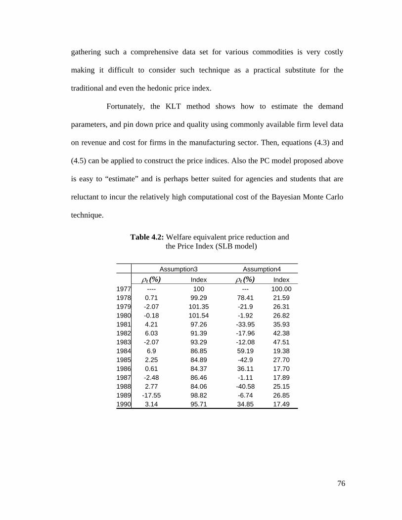
gathering such a comprehensive data set for various commodities is very costly
making it difficult to consider such technique as a practical substitute for the
traditional and even the hedonic price index.
Fortunately, the KLT method shows how to estimate the demand
parameters, and pin down price and quality using commonly available firm level data
on revenue and cost for firms in the manufacturing sector. Then, equations (4.3) and
(4.5) can be applied to construct the price indices. Also the PC model proposed above
is easy to “estimate” and is perhaps better suited for agencies and students that are
reluctant to incur the relatively high computational cost of the Bayesian Monte Carlo
technique.
Table 4.2: Welfare equivalent price reduction and the Price Index (SLB model)
Assumption3 Assumption4 ρt (%) Index ρt (%) Index 1977 ---- 100 --- 100.00 1978 0.71 99.29 78.41 21.59 1979 -2.07 101.35 -21.9 26.31 1980 -0.18 101.54 -1.92 26.82 1981 4.21 97.26 -33.95 35.93 1982 6.03 91.39 -17.96 42.38 1983 -2.07 93.29 -12.08 47.51 1984 6.9 86.85 59.19 19.38 1985 2.25 84.89 -42.9 27.70 1986 0.61 84.37 36.11 17.70 1987 -2.48 86.46 -1.11 17.89 1988 2.77 84.06 -40.58 25.15 1989 -17.55 98.82 -6.74 26.85 1990 3.14 95.71 34.85 17.49
76

With fixed quality for the outside good (assumption3), the consumer
surplus variation implies (according to the SLB model14) an equivalent price
reduction of only 4.29 % (see table above) throughout the sample period. It means
that at the end of 1990 consumers demand a reduction in prices of 4.29% 15 to go
back to 1977 set of products. Instead, if ξ0t is allowed to fluctuate (assumption4) the
welfare gains are much more significant. Now, only a sizeable 82.51% would
convince consumers to return to 1977 set of products.
Which assumption is more suitable is largely an empirical matter and
depends on the idiosyncrasies of each market. The numbers above suggest that
assumption 3 is more consistent with the beer market since consumers’ tastes are not
expected to change considerably over time. On the other hand, Assumption 4 may be
more reasonable for other markets where the imported good is much more likely to
exhibit significant temporal variation. For example, in some industries, like
automobile production in developing countries, it is likely that the quality level of
domestically produced cars lags behind the quality of imported vehicles.
4.4 Final Remarks
The first two experiments show that higher competition, through lower
import prices in the first experiment and through a new ownership arrangement in the
second, generates gains for the consumer and losses for producers. All these effects
are driven by lower prices since quality and marginal cost are kept constant. The
14 The other models present similar results, which are presented in Tables 4.8 and 4.9. 15 To obtain this number just subtract the 1977 from the 1990 indices.
77

exception is the counterfactual scenario where marginal cost is allowed to vary as a
result of the monopoly break-up. But even then, price reductions are drastic such that
consumers still enjoy significantly higher welfare.
All counterfactual experiments however ignore non-price competition
dimensions that could change the welfare figures, although it is not clear in what
direction. The Pakes-Macguire framework seems a good lead to investigate such
effects. However, more detailed data on investments (in R&D or advertising) is
necessary. Besides the computational burden, econometric estimation is also an issue
when dealing with more sophisticated dynamic models. Therefore, despite a few
drawbacks, the KLT estimation model and its variations proposed in the last chapter
constitute a useful tool for applied research in industrial organization as illustrated in
this chapter.
78

References
Lu S. and Tybout, J. (2000) “Import-Competition And Industrial Evolution: A
Computational Experiment”. Mimeo. Penn State University.
Nevo, A. (2000) “Mergers With Differentiated Products: The Case of the Ready-to-eat Cereal Industry”. RAND Journal of Economics, 31(3), pp.395-421.
Pakes, A., Berry, S. and Levinsohn, J. (1993) “Applications and Limitations of some
Recent advances in Empirical Industrial Organization: Price indexes and the Analysis of Environmental Change” American Economic Review, Papers and Proceedings 83.
Schmalensee, R. (1978) “Entry Deterrence in the Ready-to Eat Breakfast Cereal
Industry”. Bell Journal of Economics (9), pp. 305-327. Trajtenberg, M. (1990). Economic Analysis of Product Innovation: The Case of CT
Scanners, Harvard University Press, Cambridge, MA.
79

Table 4.3: Market shares and price variation as a result of the monopoly break-up and 5% marginal cost increase (NLB).
Plant ID
Ownership after break-up
Ownership before break-up
Market shares before break-up in %
Market shares gain in %
Price variation in %
1 A BAV 1.986 -1.8656 -57.691 2 A BAV 2.056 -1.8733 -58.799 3 A BAV 4.645 -3.5979 -61.647 4 A BAV 0.474 -0.4742 -16.655 5 A BAV 2.510 -2.3229 -58.292 6 A BAV 3.847 -3.8438 -47.726 7 A BAV 1.971 -1.9015 -56.197 8 A BAV 3.778 -3.2952 -59.885 9 B BAV 2.214 -1.9228 -59.958 10 B BAV 2.055 -1.842 -59.251 11 B BAV 4.495 -4.4954 -29.780 12 B BAV 1.679 -1.6788 -20.717 13 B BAV 1.121 -1.0849 -55.940 14 B BAV 0.596 0.7153 -69.807 15 C BAV 22.091 5.1295 -84.189 16 D BAV 1.379 -1.3411 -56.181 17 D BAV 3.206 6.6311 -72.176 18 D BAV 9.143 -6.9047 -62.672 19 E BAV 19.446 -18.2325 -57.760 20 D BAV 5.037 4.3042 -70.076 Other important Measures Consumer surplus variation 5478825.9 Producer surplus variation -5209736.8 Social Surplus variation 269089.14 Average prices variation 0.48715174 Column 2 presents the fictitious denominations (A, B, C, D and E) for the firms that are created after the split up. Before all plants (identified in column1) belong to Bavaria (BAV). The fifth column, in turn, presents the slice of the market they add to their previous shares. The welfare measures are all in 1975 Colombian pesos.
80

Table 4.4: Market shares and price variation as a result of the monopoly break-up (SLB)
Plant ID
Ownership after break-up
Ownership before break-up
Market shares before break-up in %
Market shares gain in %
Price variation in %
1 A BAV 1.994 0.072 -55.421 2 A BAV 2.065 0.0746 -56.399 3 A BAV 4.666 0.1686 -58.918 4 A BAV 0.476 0.0172 -19.143 5 A BAV 2.521 0.0911 -55.952 6 A BAV 3.864 0.1396 -46.611 7 A BAV 1.979 0.0715 -54.099 8 A BAV 3.795 0.1371 -57.359 9 B BAV 2.223 0.3693 -57.853 10 B BAV 2.064 0.3429 -57.223 11 B BAV 4.515 0.75 -30.975 12 B BAV 1.686 0.2801 -22.904 13 B BAV 1.126 0.1869 -54.274 14 B BAV 0.599 0.0995 -66.624 15 C BAV 22.189 0.5654 -79.575 16 D BAV 1.385 0.0964 -54.243 17 D BAV 3.220 0.224 -68.423 18 D BAV 9.183 0.6388 -59.996 19 E BAV 19.532 1.1777 -55.560 20 D BAV 5.060 0.3519 -66.562 Other important Measures Consumer surplus variation 5170125.3 Producer surplus variation - 4862150.4 Social Surplus variation 307974.93 Average Price variation -47.64% Column 2 presents the fictitious denominations (A, B, C, D and E) for the firms that are created after the split up. Before all plants (identified in column1) belong to Bavaria (BAV). The fifth column, in turn, presents the slice of the market they add to their previous shares. The welfare measures are all in 1975 Colombian pesos.
81
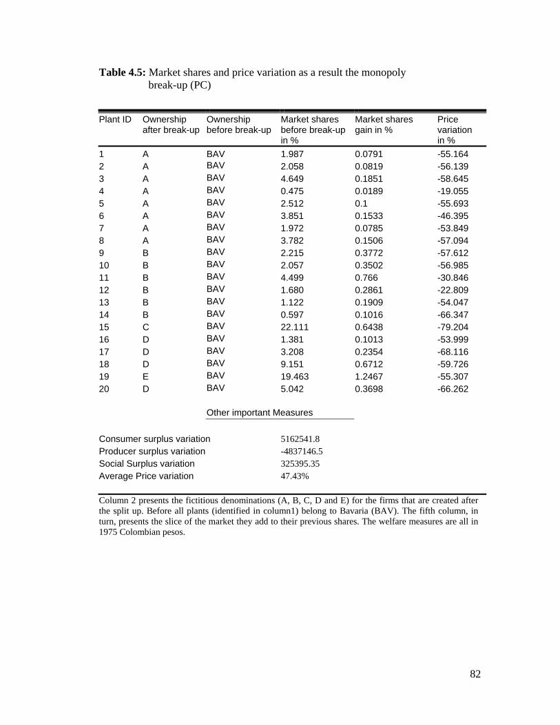
Table 4.5: Market shares and price variation as a result the monopoly break-up (PC)
Plant ID
Ownership after break-up
Ownership before break-up
Market shares before break-up in %
Market shares gain in %
Price variation in %
1 A BAV 1.987 0.0791 -55.164 2 A BAV 2.058 0.0819 -56.139 3 A BAV 4.649 0.1851 -58.645 4 A BAV 0.475 0.0189 -19.055 5 A BAV 2.512 0.1 -55.693 6 A BAV 3.851 0.1533 -46.395 7 A BAV 1.972 0.0785 -53.849 8 A BAV 3.782 0.1506 -57.094 9 B BAV 2.215 0.3772 -57.612 10 B BAV 2.057 0.3502 -56.985 11 B BAV 4.499 0.766 -30.846 12 B BAV 1.680 0.2861 -22.809 13 B BAV 1.122 0.1909 -54.047 14 B BAV 0.597 0.1016 -66.347 15 C BAV 22.111 0.6438 -79.204 16 D BAV 1.381 0.1013 -53.999 17 D BAV 3.208 0.2354 -68.116 18 D BAV 9.151 0.6712 -59.726 19 E BAV 19.463 1.2467 -55.307 20 D BAV 5.042 0.3698 -66.262 Other important Measures Consumer surplus variation 5162541.8 Producer surplus variation -4837146.5 Social Surplus variation 325395.35 Average Price variation 47.43% Column 2 presents the fictitious denominations (A, B, C, D and E) for the firms that are created after the split up. Before all plants (identified in column1) belong to Bavaria (BAV). The fifth column, in turn, presents the slice of the market they add to their previous shares. The welfare measures are all in 1975 Colombian pesos.
82

Table 4.6: Market shares and price variation as a result of the monopoly break-up (scenario 1)
Plant ID
Ownership after break-up
Ownership before break-up
Market shares before break-up in %
Market shares gain in %
Price variation in %
1 A BAV 1.986 0.2578 -47.314 2 A BAV 2.056 0.267 -48.150 3 A BAV 4.645 0.6033 -50.299 4 A BAV 0.474 0.0616 -16.343 5 A BAV 2.510 0.326 -47.767 6 A BAV 3.847 0.4996 -39.793 7 A BAV 1.971 0.2559 -46.186 8 A BAV 3.778 0.4907 -48.970 9 A BAV 2.214 0.2875 -49.024 10 A BAV 2.055 0.267 -48.490 11 A BAV 4.495 0.5838 -26.248 12 A BAV 1.679 0.2181 -19.409 13 A BAV 1.121 0.1455 -45.992 14 A BAV 0.596 0.0774 -56.457 15 B BAV 22.091 0.2957 -67.945 16 C BAV 1.379 0.1791 -46.215 17 C BAV 3.206 0.4163 -58.298 18 B BAV 9.143 0.1224 -51.092 19 B BAV 19.446 0.2604 -47.339 20 C BAV 5.037 0.6542 -56.712 Other important Measures Consumer surplus variation 4442218.9 Producer surplus variation - 4089412.5 Social Surplus variation 352806.44 Average Price variation 40.56% Column 2 presents the fictitious denominations (A, B, C) for the firms that are created after the split up. Before all plants (identified in column1) belong to Bavaria (BAV). The fifth column, in turn, presents the slice of the market they add to their previous shares. The welfare measures are all in 1975 Colombian pesos.
83
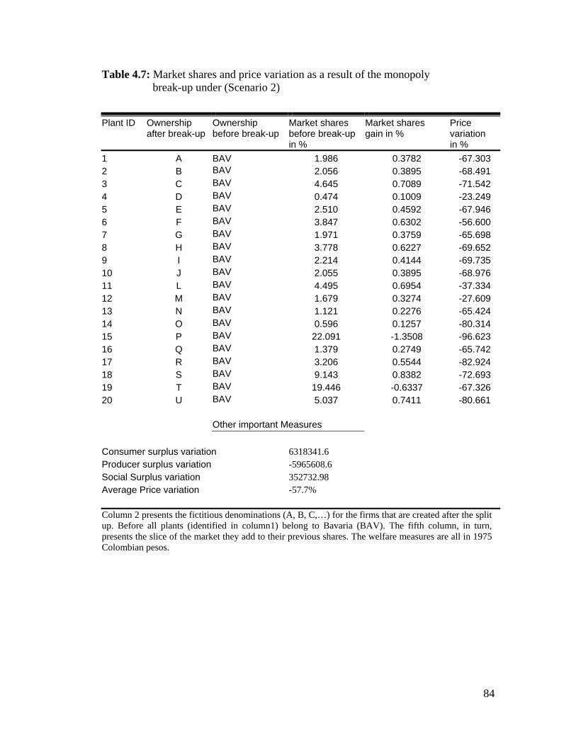
Table 4.7: Market shares and price variation as a result of the monopoly break-up under (Scenario 2)
Plant ID
Ownership after break-up
Ownership before break-up
Market shares before break-up in %
Market shares gain in %
Price variation in %
1 A BAV 1.986 0.3782 -67.303 2 B BAV 2.056 0.3895 -68.491 3 C BAV 4.645 0.7089 -71.542 4 D BAV 0.474 0.1009 -23.249 5 E BAV 2.510 0.4592 -67.946 6 F BAV 3.847 0.6302 -56.600 7 G BAV 1.971 0.3759 -65.698 8 H BAV 3.778 0.6227 -69.652 9 I BAV 2.214 0.4144 -69.735 10 J BAV 2.055 0.3895 -68.976 11 L BAV 4.495 0.6954 -37.334 12 M BAV 1.679 0.3274 -27.609 13 N BAV 1.121 0.2276 -65.424 14 O BAV 0.596 0.1257 -80.314 15 P BAV 22.091 -1.3508 -96.623 16 Q BAV 1.379 0.2749 -65.742 17 R BAV 3.206 0.5544 -82.924 18 S BAV 9.143 0.8382 -72.693 19 T BAV 19.446 -0.6337 -67.326 20 U BAV 5.037 0.7411 -80.661 Other important Measures Consumer surplus variation 6318341.6 Producer surplus variation -5965608.6 Social Surplus variation 352732.98 Average Price variation -57.7% Column 2 presents the fictitious denominations (A, B, C,…) for the firms that are created after the split up. Before all plants (identified in column1) belong to Bavaria (BAV). The fifth column, in turn, presents the slice of the market they add to their previous shares. The welfare measures are all in 1975 Colombian pesos.
84

Table 4.8: Welfare equivalent price reduction the Price Index (NLB model)
Assumption3 Assumption4 ρt (%) Index ρt (%) Index 1977 --- 100.00 100.00 1978 0.42 99.57 77.71 22.29 1979 -1.72 101.29 -21.49 27.08 1980 -0.2 101.50 -1.88 27.59 1981 3.48 97.97 -34.78 37.19 1982 5.79 92.29 -18.25 43.97 1983 -1.9 94.04 -11.84 49.18 1984 5.24 89.11 57.52 20.89 1985 1.34 87.91 -45.62 30.42 1986 1.26 86.80 38.3 18.77 1987 -2.15 88.67 -0.5 18.86 1988 1.23 87.57 -44.37 27.23 1989 -14.46 100.24 -1.06 27.52 1990 2.6 97.63 39.37 16.69
85

Table 4.9 : Welfare equivalent price reduction the Price Index (PC model)
Assumption3 Assumption4 ρt (%) Index ρt (%) Index 1977 ---- 100 100 100.00 1978 4.43 95.56 84.86 15.13 1979 0.06 95.50 -27.32 19.27 1980 -1.11 96.56 0.16 19.23 1981 -1.49 98.00 -34.87 25.94 1982 -0.6 98.60 -19 30.87 1983 -4.75 103.29 -15.2 35.57 1984 1.64 101.59 69.09 10.99 1985 0.83 100.74 -42.41 15.66 1986 -2.17 102.93 27.77 11.31 1987 -6.53 109.66 -9.31 12.36 1988 13.78 94.54 -15.92 14.33 1989 -13.15 106.98 -10.35 15.81 1990 -0.63 107.65 -1.75 16.09
86

Appendix A: Uncovering relevant quantities from Revenue and Cost data with Multi-Plant Ownership.
This appendix shows how to uncover relevant plant-level quantities
from revenue and cost data using up to some parameters of the model. Equation (3.5)
in the text can be rewritten as
(A1. 1) 0)(1 =∂∂
−+ ∑∈ fFr
jj
rrr s
ps
mcp
Further, is easy to show that the following equalities hold for the cross
and own price derivatives
])1([1 wj
j
rj
j
r sssss
ps
σσσ
α−−−
−−=
∂∂
])1(1[1 wjj
j
j sssps
σσσ
α−−−
−−=
∂
∂
Note that jrjr qqss = , Rj=pj.qj, TCj=mcj.qj, and sj=qj/(Q+Q0)
where Rj ,TCj, Q and Q0 are revenue, total variable cost, total output produced by
domestic firms and total imported quantity respectively. Hence, substituting these
equations into the pricing rule and solving for quantity of plant j belonging to firm f
(j∈ Ff ) one obtains
(A1. 2)
1
0 )()(
.)1().(
1−
∈ ⎟⎟
⎠
⎞
⎜⎜
⎝
⎛⎟⎟⎠
⎞⎜⎜⎝
⎛
−−
⎟⎟⎠
⎞⎜⎜⎝
⎛+
+−
+−−
= ∑fFr jj
rr
jjj TCR
TCRQQQTCR
q σσα
σ
87

Aggregating over the qj’s results in
1
0,..2,1 )()(
.)1().(
1−
∈∈= ⎟⎟
⎠
⎞
⎜⎜
⎝
⎛⎟⎟⎠
⎞⎜⎜⎝
⎛
−−
⎟⎟⎠
⎞⎜⎜⎝
⎛+
+−
+−−
= ∑∑∑ff Fr jj
rr
jjFjNFf TCRTCR
QQQTCRQ σσ
ασ
where NF is the total number of firms. This non-linear equation can be
solved numerically for Q given (α,σ,Rj ,TCj,Q0). Then, given the same parameters
and data, qj is determined (A1. 2), whereas pj , mcj , sj and sw follow trivially from
jjj qRp = , jjj qTCmc = , sj=qj/(Q+Q0) and sw=qj/Q respectively.
Finally, the log-linearized version of the demand system (3.7) can be
solved for relative quality aj
000 lnlnln).( sssppa jwjjjt −+−−=−≡ σαξξ
88

Appendix B: Gibbs sampler16
Although, one cannot make inference directly from )().;( θθ pDL , it is
possible to sample from the full conditionals of the θ components. In the NLB model,
the parameter vector is divided into: ),(),(),(),,( 4321 σαθνθθλϕθ ==Σ== . The
parameters σαλϕ ,,, are defined as before, Σ is the covariance matrix of the VAR
error terms and ν is the variance of error in the aggregate quantity equation (3.10).
The Gibbs algorithm goes as follows.
Step 0: Draw initial values for the parameter vector
and set i=0. ),,,( 04
03
02
01
0 θθθθθ =
Step 1: Draw from the conditionals below. 1+iθ
1.1) Draw ),,,|(~ 432111
1 Diiii θθθθπθ +
1.2) Draw ),,,|(~ 431
1221
2 Diiii θθθθπθ ++
1.3) Draw ),,,|(~ 41
21
1331
3 Diiii θθθθπθ +++
1.4) Draw ),,,|(~ 13
12
1144
14 Diiii ++++ θθθθπθ
Step 2: Set i=i+1 and go back to step 1.
16 This appendix is heavily based on KLT (2003) and is included in this work for the sake of clarity.
89

Here , where )().;(),|( kkkkk pDLD θθθθπ θ=− )( kkp θθ is the prior of the
sub-vector θk. Further, to describe the conditionals, define
, , , and . )'( , jtjtjt mcaY = )',,,1( tmcaZ jtjtjt = )',( cjt
ajtjtU εε= ⎟
⎟⎠
⎞⎜⎜⎝
⎛=
φλλ
βϕϕc
c
b
bB
02
01'
In addition, let
]'................[ 2112 NTNT YYYYY = ,
]'................[ 2112 NTNT ZZZZZ = ,
]'..................[ 2112 NTNT UUUUU =
The VAR system can then be written as Y=XB+U. Given , Y and Z are
given and 1.1) to 1.3) have known probability distributions. On the other hand,
does not have a closed from solution, which requires the use of
a Metropolis-Hastings (M-H) algorithm.
4θ
),,,|( 32144 Dθθθθπ
More specifically, defining K as one plus the number of variables
appearing on the RHS of the VAR and assuming that the prior of θ1 is
, one can show that (1π also a normal with mean
[ ](un = ariance
)100,0( 22 kk IN × ),,,| 4321 Dθθθθ is
YVecZ Σ⊗ and v)'()' [ ] 12
1 )100/1())'(( −− +Σ⊗=nV kIZZ
For 1.2 it is assumed that Σ has Inverse Wishart prior with parameters 6
and 100xI2. Then has a distribution , where
m
),,,|( 43122 Dθθθθπ ),( 1−nn GmInvWish
n = 6 + number of observations17, and . )()'()100( 21 ZBYZBYIGn −−+×=−
17 Adjusted for the lags
90

Similarly, ν has the prior distribution defined as the scalar version of the
inverse Wishart (InvWish(6,100) ). Hence, the conditional is
also a , m
),,,|( 42133 Dθθθθπ
),( 1−nn GmInvWish n= 6 + (np-1), and , where w is a vector
that collects all the w
wwGn '1001 +=−
t’s.
The prior for α is a uniform with support [0,10], while σ has the same
prior but its support is a little narrower [0,1]. Since one cannot identify the shape of
, has to be sampled using a random walk Metropolis-
Hastings acceptance criterion with a normal proposal density. The probability of
acceptance of is
),,,|( 32144 Dθθθθπ 4θ
'4θ
⎭⎬⎫
⎩⎨⎧
+++
+++
),,,|(),,,|(
,1min 13
12
1144
13
12
11
'44
DD
iiii
iii
θθθθπθθθθπ , where is drawn from a
normal density with mean and variance Λ. In principle, any Λ can be used in the
algorithm, however, for a well behaved convergence to the invariant probability
distribution, it is recommended to calibrate this variance such that it is not too “big”
(all the proposed will be accepted but the chain will move slowly) nor too “small”
(nearly all proposed moves will be rejected and the chain may not move for several
iterations).
'4θ
i4θ
'4θ
Once convergence of the Markov chain has been attained (suppose at the
Lth simulation) it suffices to sample from the invariant distribution using the draws
, where i >L. To obtain the statistics reported in Table 3.1, I run 20000 iterations of
the Markov chain and set L to be 2000. Figures 3.1 to 3.3 at the end of chapter 3 show
the graphs of the MCMC simulations for the demand parameters for both the SLB
iθ
91

and the NLB models. Clearly, after 2000 iterations the Markov chain moves within a
certain range and inference can be made from then on.
92

Curriculum Vita
Sergio Aquino DeSouza Av. Sen. Virgilio Tavora 233, apt. 802, Fortaleza-CE 60170250 , Brazil
Telephone: 55-85-2425207 E-mail: [email protected]
Education:
• PhD., Economics, The Pennsylvania State University, December 2004
• M.A., Economics, Universidade Federal do Ceará, June 2000
Fields of Interest:
• Applied Microeconomics, Industrial Organization, Econometrics and International Trade
Working Paper:
• “Describing Firm’s Behavior Using Revenue and Cost Data”
Professional Experience:
• Teacher Assistant, The Penn State University, August 2001 to May 2004.
• Instructor for Statistics, Universidade Federal do Ceará, June 1999 to June 2000
Awards:
• CAPES Fellowship • CNPq Fellowship