arX

iv:1

102.

2258

v1 [

mat

h-ph

] 1

0 Fe

b 20

11

Generalized Local Induction Equation, Elliptic Asymptotics, and Simulating

Superfluid Turbulence

Scott A. Strong and Lincoln D. Carr1

Department of Physics

Colorado School of Mines

Golden, CO 80401, U.S.A.

(Dated: 13 June 2018)

We prove the generalized induction equation and the generalized local induction equa-

tion (GLIE), which replaces the commonly used local induction approximation (LIA)

to simulate the dynamics of vortex lines and thus superfluid turbulence. We show

that the LIA is, without in fact any approximation at all, a general feature of the

velocity field induced by any length of a curved vortex filament. Specifically, the LIA

states that the velocity field induced by a curved vortex filament is asymmetric in the

binormal direction. Up to a potential term, the induced incompressible field is given

by the Biot-Savart integral, where we recall that there is a direct analogy between

hydrodynamics and magnetostatics. Series approximations to the Biot-Savart inte-

grand indicate a logarithmic divergence of the local field in the binormal direction.

While this is qualitatively correct, LIA lacks metrics quantifying its small parame-

ters. Regardless, LIA is used in vortex filament methods simulating the self-induced

motion of quantized vortices. With numerics in mind, we represent the binormal

field in terms of incomplete elliptic integrals, which is valid for R3. From this and

known expansions we derive the GLIE, asymptotic for local field points. Like the

LIA, generalized induction shows a persistent binormal deviation in the local-field

but unlike the LIA, the GLIE provides bounds on the truncated remainder. As an

application, we adapt formulae from vortex filament methods to the GLIE for future

use in these methods. Other examples we consider include vortex rings, relevant for

both superfluid 4He and Bose-Einstein condensates.

1

I. INTRODUCTION

The term superfluid denotes a phase of matter whose dynamical flows can be described,

at finite non-zero temperature, by a two-component macroscopic field with well-defined

properties.1–3 One component is a purely classical field, while what remains is called the

superfluid component. The superfluid is ideal in the sense that it is inviscid and has infinite

heat capacity provided by its lack of classical entropy. Rotation enters the superfluid compo-

nent in quantized vortex filaments4,5 that, for example in 4He, transmit thermal information

acoustically and are detected by this second-sound.6 Superfluid dynamics can be generated

by the introduction of a small heat flux.7 Conservation of mass requires that the classical

movement away from the heat flux be offset by a counterflow of the superfluid component.

If this heat flux is not small, then the quantized vortices tangle, indicating the onset of

superfluid turbulence.8–13 For large heat fluxes, the superfluid transitions into a purely clas-

sical phase. In classical turbulence, vorticity can concentrate into complicated geometries.

For this reason, large-scale simulation of classical vortex dominated flows is computationally

costly.

Vortex line structures are most appropriate to superfluid models of 4He where the quan-

tized filaments have radii of a few angstroms.6,14 These quantized vortices provide a coherent

structure for aggressive analytical and numerical study unavailable to classical fluids. Vor-

tex line structures can also be used to model atomic Bose-Einstein condensates, where there

has recently been a revival of interest in superfluid turbulence due in part to a series of

remarkable experiments in the Bagnato group.15 Our study begins with simplifications to

the Biot-Savart representation of the field induced by a vortex line

v(x) =Γ

4π

∫

D⊂R3

(x− ω)× dω

|x− ω|3 =Γ

4π

∫

D⊂R

(x− ξ)× dξ

|x− ξ|3 . (1)

The associated reduction of dimension aids analytic calculation and reduces numerical cost.

When such filaments are considered initial-data to the Navier-Stokes problem, then global

well-posedness results.16,17 The use of these data to approximate self-induced vortex motion

is the backbone of the vortex filament method.18,19 The question of numerical convergence

and accuracy of such vortex filament techniques has been addressed affirmatively in the

literature.20 Vortex filament methods reduce the cost of large-scale simulations by restricting

analysis to the local field. Due to the complexity of classical vortical flows, interest in these

methods waned during the 1980s.18,19,21–23 However, filament methods are highly appropriate

2

for the constrained vortex structure associated with a superfluid. Although (1) provides a

straightforward starting point for numerical computations, vortex filament methods avoid

numerical integration altogether by replacing (1) with a local induction approximation.

The local induction approximation (LIA) is a result from classical fluid dynamics, which

states that a space-curve vortex defect of an incompressible fluid field with nontrivial cur-

vature generates a binormal asymmetry in the local velocity field. That is, the field local to

a length of curved vortex filament induces a flow, which generates filament dynamics. This

result, known by Tullio Levi-Civita and his student Luigi Sante Da Rios in the early 1900’s,24

was rediscovered by various post World-War II groups.25–28 Together, Ricca29 and Hama30

provide an excellent chronology of LIA, a topic now common in vortex dynamics texts.17,31,32

Exploration of LIA occurs in various settings including differential geometry,33–45 differential

equations25 and limits of matched asymptotic expansions of vortex tubes.26,28,46

Our derivation avoids the complications of matched asymptotic expansions by treating

vorticity concentrated to an arc. Under this geometry Eq. (1) can be reduced to a canonical

elliptic representation without the use of power-series approximation to the Biot-Savart

integrand.27,47 While Taylor approximation quickly reveals binormal flow as a dominant

feature of the induced field, it lacks error bounds and is often restricted to a two-dimensional

subspace of R3. This paper resolves both issues by recasting Eq. (1), for a vortex-arc,

into an elliptic form valid for all field points. Using this form, one can then use a known

asymptotic formula to represent the local field. We offer that this should be adopted, instead

of LIA, for use in vortex filament methods and Schwarz’s description of the Magnus force.14,48

Specifically, we will prove the following results:

Theorem 1 Generalized Induction Equation

Let ω = ∇ × v be localized to an arbitrary arc with parameterization ξ = (R sin(θ), R −R cos(θ), 0), where R ∈ R

+ and θ ∈ DL = (−L, L] for some L ∈ (−π, π]. Then there exists

bounded functions V1, α1, α2, L± and k, of ε = |x|/R = κ|x|, such that the induced velocity

field is given by

v(x) = V1(ε)

(

α1(ε) [F (L+, k)− F (L−, k)] + α2(ε)

[

dF (L+, k)

dε− dF (L−, k)

dε

])

(2)

where F is an incomplete elliptic integral of the first kind. Moreover, there exist constants

3

β1, β2, β3, β4 such that V1 can be written as

V1(ε) = εβ1t− εβ2n+ (εβ2 + εβ3 + β4) b (3)

where t, n, b, are the tangent, normal and binormal vectors of the local coordinate system.

Theorem 2 Generalized Local Induction Equation

Under the same hypotheses of theorem 1 and for ε ≪ 0 the induced velocity field is dominated

by the binormal flow,

vε(x) = 4κx2

(

α1(ε) [F (L+, k)− F (L−, k)] + α2(ε)

[

dF (L+, k)

dε− dF (L−, k)

dε

])

b. (4)

where x2 is a dimensionless angular component of the spherical decomposition of x and κ

is the curvature of the vortex arc. The limits ε → 0 and L → 0 imply that k → 1 and

λ→ 0 and in this case the incomplete elliptic integral of the first kind admits the asymptotic

relation F ∼ F1 where

F1(λ, k) = ln

(

√

1 + λ

1− λ

)

+1

λln

(

2

1 +√

(1− k2λ2)/(1− λ2)

)

+1− k2

8ln

(

1 + λ

1− λ

)

. (5)

Using this, along with standard differentiation formula for incomplete elliptic integrals of the

first kind, provides a first order asymptotic form for the local field given by

vε(x) ∼ −8κx2

9x2F1(λ, k)

2− x2E(L, k)

(1 − k2)k−k sin(2L)

[

√

1 + k2 sin2(L) +√

1− k2 sin2(L)]

2(1− k2)√

1− k4 sin4(L)

b,

(6)

where E is an incomplete elliptic integral of the second kind.

In words, the first theorem expresses the velocity field generated by vortex arc in terms

of incomplete elliptic integrals of the first kind. Moreover, this field can be decomposed

into three fields controlling the tangential, circulatory and binormal flows. Of these fields,

the binormal contribution is O(1) while the remaining fields are O(ε). The second theorem

considers the remaining field in the limits of ε → 0 and L → 0. In this limit the incomplete

elliptic integral of the first kind admits an asymptotic form and consequently provides a

representation for the velocity field local to the vortex arc. This asymptotic form is com-

parable to LIA in that the Biot-Savart integral has been ‘resolved’ and the binormal flow is

represented by elementary functions. This form is only valid for filaments of infinitesimal

4

arclength and consequently idealized. However, using the same asymptotic framework, one

can construct expansions valid for arcs of finite length. In fact, the remainder terms of such

expansions are known and thus the associated approximation error can be controlled. The

necessary asymptotic results are quoted in the appendix.

The rest of this document will be organized as follows. In Section II we define the

geometry and derive the Biot-Savart representation of the induced velocity field. In Section

III we convert this representation into an elliptic form and prove the generalized induction

result (2)-(3). In Section IV we reduce this elliptic form into a sum of incomplete elliptic

integrals of the first kind. Lastly, using known asymptotic results, we derive an expression

for the local velocity field and prove the generalized local induction equation (GLIE) result

(6). We conclude with some discussion on adapting this result to vortex filament methods

and prospective avenues of future work.

II. BIOT-SAVART AND QUANTIZED VORTEX RINGS

It is well known that a vortex-defect with trivial curvature embedded into an incompress-

ible fluid does not induce autonomous dynamics. This is due to an angular symmetry in

the induced velocity field. This symmetry is no longer available for curved vortex elements.

Using a vortex ring, it is possible to introduce nontrivial curvature and avoid approximations

to the Biot-Savart integral. To be precise, we treat a vortex structure ω : R3 → R3 such

that

ω(x) =

1, x ∈ ξ

0, x /∈ ξ(7)

where ξ : D → R3, D ⊂ R, is parameterized by the ring

ξ = R sin(θ)i+ [R −R cos(θ)] j, (8)

dξ =[

R cos(θ)i+R sin(θ)j]

dθ (9)

for κ−1 = R ∈ R+, DL = (−L, L] and L ∈ [0, π]. Thus, at the point x = (x1, x2, x3) we get

an element level description of the velocity field,

vi(x) =

∫

DL

ǫijk(xj − ξj)dξk

[|x|2 + |ξ|2 − 2(x1ξ1 + x2ξ2 + x3ξ3)]3/2

(10)

5

where we have used the Levi-Civita symbol, ǫijk, and employed silent-summation over re-

peated indices. Noting that |ξ|2 = 2R2 − 2R2 cos(θ) provides the formulae

v1 = −|x|κ2x3∫

DL

sin(θ)

D3/2dθ, (11)

v2 = |x|κ2x3∫

DL

cos(θ)

D3/2dθ, (12)

v3 = κ2|x|∫

DL

x1 sin(θ)− x2 cos(θ)

D3/2dθ + κ

∫

DL

cos(θ)− 1

D3/2dθ (13)

where the denominator is given by

D = [c1 + c2 cos(θ) + c3 sin(θ)] (14)

and whose coefficients are

R2c1 = |x|2 + 2R2 − 2x2R, (15)

R2c2 = 2|x|x2R− 2R2, (16)

R2c3 = −2|x|x1R. (17)

For future limiting work, we have chosen a radial-representation for x = |x|(x1, x2, x3) wherexi is the i

th dimensionless angular component of x.

III. CONVERSION TO ELLIPTIC FORM

The previous integral representations for the velocity field can be cast into elliptic form.

To do this, we first reduce each integral into an elliptic integral by taking derivatives with

respect to internal parameters. Doing so gives

v1 = 2κx3εd

dc3

∫

DL

dθ√D, (18)

v2 = −2κx3εd

dc2

∫

DL

dθ√D, (19)

v3 =

[

2κεx2d

dc2− 2κεx1

d

dc3+ 2κ

d

dc1− 2κ

d

dc2

]∫

DL

dθ√D

(20)

where the parameter ε = |x|/R is the ratio of radial distance to the radius of curvature.

Application of the chain-rule gives the induced velocity field as

v(x) = V1(ε)d

dε

∫

DL

dθ√D

(21)

6

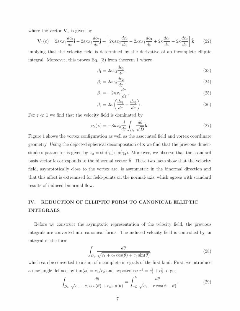
where the vector V1 is given by

V1(ε) = 2εκx3dc3dε

i− 2εκx2dc2dε

j +

[

2κεx2dc2dε

− 2κεx1dc3dε

+ 2κdc1dε

− 2κdc2dε

]

k (22)

implying that the velocity field is determined by the derivative of an incomplete elliptic

integral. Moreover, this proves Eq. (3) from theorem 1 where

β1 = 2κx3dc3dε, (23)

β2 = 2κx2dc2dε, (24)

β3 = −2κx1dc3dε, (25)

β4 = 2κ

(

dc1dε

− dc2dε

)

. (26)

For ε≪ 1 we find that the velocity field is dominated by

vε(x) = −8κx2d

dε

∫

DL

dθ√Dk. (27)

Figure 1 shows the vortex configuration as well as the associated field and vortex coordinate

geometry. Using the depicted spherical decomposition of x we find that the previous dimen-

sionless parameter is given by x2 = sin(γ1) sin(γ2). Moreover, we observe that the standard

basis vector k corresponds to the binormal vector b. These two facts show that the velocity

field, asymptotically close to the vortex arc, is asymmetric in the binormal direction and

that this affect is extremized for field-points on the normal-axis, which agrees with standard

results of induced binormal flow.

IV. REDUCTION OF ELLIPTIC FORM TO CANONICAL ELLIPTIC

INTEGRALS

Before we construct the asymptotic representation of the velocity field, the previous

integrals are converted into canonical forms. The induced velocity field is controlled by an

integral of the form∫

DL

dθ√

c1 + c2 cos(θ) + c3 sin(θ), (28)

which can be converted to a sum of incomplete integrals of the first kind. First, we introduce

a new angle defined by tan(φ) = c3/c2 and hypotenuse r2 = c22 + c23 to get∫

DL

dθ√

c1 + c2 cos(θ) + c3 sin(θ)=

∫ L

−L

dθ√

c1 + r cos(φ− θ). (29)

7

x

y

z

b

b

ξ

x = |x|(x1, x2, x3)

γ1

γ2

t

n

b

b

b

−L

L

C

(a) Vortex Configuration

x

y

t

n

L−L

C

bb

b

ξ

R

ξ = (R sin(θ), R −R cos(θ))

θ

(b) Tangent-Normal Plane

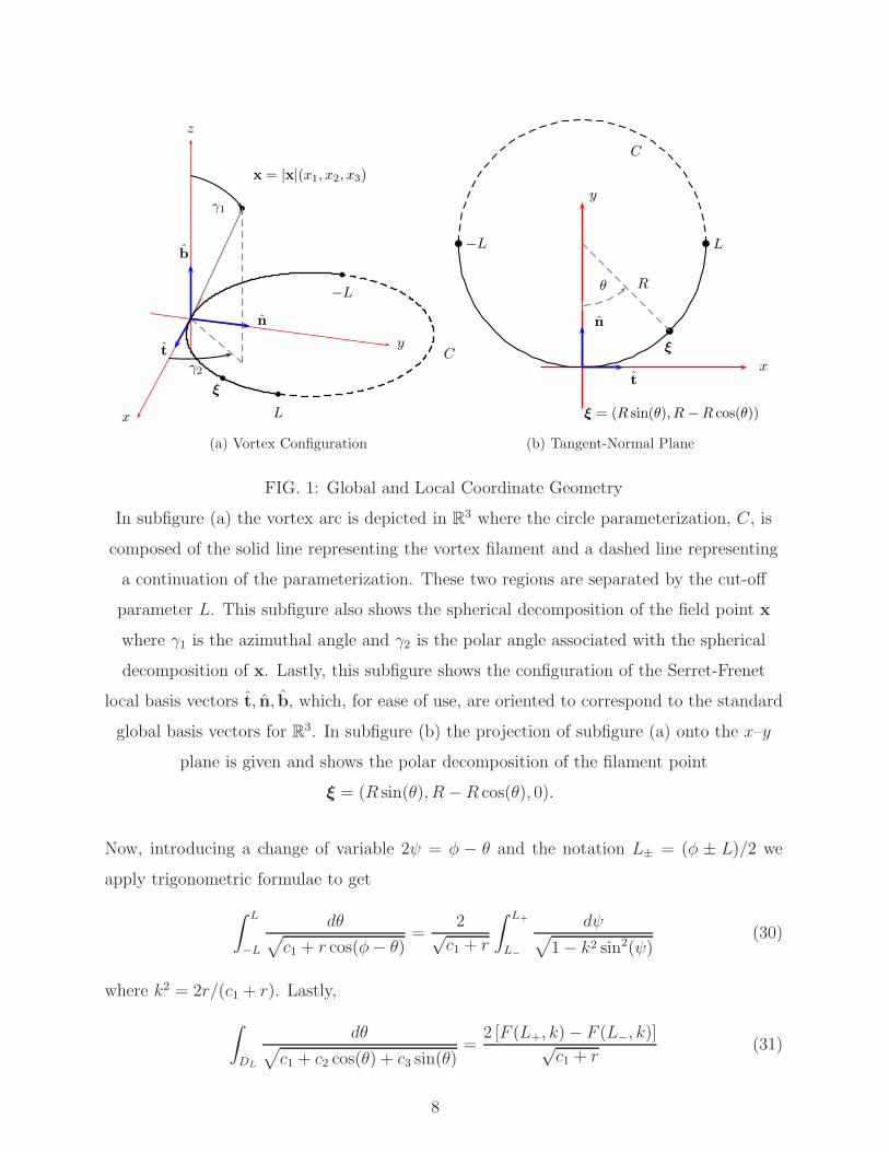
FIG. 1: Global and Local Coordinate Geometry

In subfigure (a) the vortex arc is depicted in R3 where the circle parameterization, C, is

composed of the solid line representing the vortex filament and a dashed line representing

a continuation of the parameterization. These two regions are separated by the cut-off

parameter L. This subfigure also shows the spherical decomposition of the field point x

where γ1 is the azimuthal angle and γ2 is the polar angle associated with the spherical

decomposition of x. Lastly, this subfigure shows the configuration of the Serret-Frenet

local basis vectors t, n, b, which, for ease of use, are oriented to correspond to the standard

global basis vectors for R3. In subfigure (b) the projection of subfigure (a) onto the x–y

plane is given and shows the polar decomposition of the filament point

ξ = (R sin(θ), R− R cos(θ), 0).

Now, introducing a change of variable 2ψ = φ − θ and the notation L± = (φ ± L)/2 we

apply trigonometric formulae to get

∫ L

−L

dθ√

c1 + r cos(φ− θ)=

2√c1 + r

∫ L+

L−

dψ√

1− k2 sin2(ψ)(30)

where k2 = 2r/(c1 + r). Lastly,

∫

DL

dθ√

c1 + c2 cos(θ) + c3 sin(θ)=

2 [F (L+, k)− F (L−, k)]√c1 + r

(31)

8

where F is the standard incomplete elliptic integral of the first kind,

F (ϕ, k) =

∫ ϕ

0

dψ√

1− k2 sin2(ψ)=

∫ λ

0

dt√1− t2

√1− k2t2

(32)

such that λ = sin(ϕ).

V. ASYMPTOTICS FOR THE INCOMPLETE ELLIPTIC INTEGRAL OF

THE FIRST KIND

Having reduced the Biot-Savart representation of the velocity field to a canonical form,

we can now make use of the known asymptotic formula of Karp and Sitnik,49 which permits

the study of (32) for all (λ, k) ∈ [0, 1]× [0, 1]. Specifically, they derive a series representation

and remainder term for F , which is asymptotic for k → 1. Their complete theorem is quoted

in the appendix, but we only require the first-order approximation

F1(λ, k) = ln

(

√

1 + λ

1− λ

)

+1

λln

(

2

1 +√

(1− k2λ2)/(1− λ2)

)

+1− k2

8ln

(

1 + λ

1− λ

)

. (33)

which is asymptotic to F for λ → 0 and k → 1. This asymptotic formula is not suited to

differentiation.50–53 Thus, we must first apply the differentiation formula, for the incomplete

elliptic integral of the first kind, prior to its asymptotic evaluation. Doing so gives lengthy

formulae and for these we introduce the constants

A =x2c2 − x1c3

r, (34)

A1 =−4

(c1 + r)3/2(ε− x2 + A), (35)

A2 =2√c1 + r

, (36)

A3 = −2x2c3 + x1c2

r2, (37)

A4 =

√2r(x2 − ε)

(c1 + r)3/2+

√

2

r

(

(c1 + r)3/2 − r√c1 + r

(c1 + r)2

)

A. (38)

Using these constants, find

d

dε

∫

DL

dθ√D

= 2A1[F (L+, k)− F (L−, k)] + A2 [Ω(A3, A4, A5, k, L+)− Ω(A3, A4, A5, k, L−)]

(39)

9

where

Ω(A3, A4, A5, k, L) =A3

√

1− k2 sin2(L)+A4E(L, k)

1(1− k2)k− A4F (L, k)

2k− A42k sin(2L)

4(1− k2)√

1− k2 sin2(L)

(40)

is given by differentiation formula for incomplete elliptic integrals of the first kind. Together

with Eq. (21), proves Eq. (2) of our first theorem where α1 = 2A1 and α2 = A2. From Eq.

(27) we find that the local velocity field is given by

vε(x) = −8κx2 (2A1[F (L+, k)− F (L−, k)] + A2 [Ω(A3, A4, A5, k, L+)− Ω(A3, A4, A5, k, L−)]) .

(41)

At this point, the asymptotic formula (A.1) can now be applied to F (λ, k) where λ =

sin(L±). To compare these results to standard LIA we take ε → 0 and L → 0. In this case

c1 = −c2 = r ∼ 2, c3 ∼ 0 and the constants take the asymptotic forms

A =x2c2 − x1c3

r∼ −x2, (42)

A1 =−4

(c1 + r)3/2(ε− x2 + A) ∼ x2, (43)

A2 =2√c1 + r

∼ 1, (44)

A3 = −2x2c3 + x1c2

r2∼ x1, (45)

A4 =

√2r(x2 − ε)

(c1 + r)3/2+

√

2

r

(

(c1 + r)3/2 − r√c1 + r

(c1 + r)2

)

A ∼ −x22. (46)

Together this gives the first-order asymptotic representation for the velocity field,

vε(x) ∼ −8κx2

9x2F1(λ, k)

2− x2E(L, k)

(1− k2)k−k sin(2L)

[

√

1 + k2 sin2(L) +√

1− k2 sin2(L)]

2(1− k2)√

1− k4 sin4(L)

b

(47)

for the limits ε→ 0, k → 1 and L → 0, λ → 0. This proves Eq. (6) of our GLIE. It should

be noted that the above formula is nonzero even for the extreme case of L = 1 − k → 0.

The physical meaning of this statement is that the local field induced by an infinitesimal

segment of a vortex line is nonzero and asymmetric in the binormal direction.

VI. DISCUSSION AND CONCLUSIONS

We have derived an asymptotic representation for the local velocity field induced by

a curved vortex filament. This derivation generalizes the previously known statements of

10

induced binormal flow, which play an important role in two-component superfluid simulation.

In such simulations one must calculate the superfluid and normal fluid flows as well as

their mutual friction interaction. This mutual friction embodies the scattering of rotons

and phonons off of the vortex structures.8–11,54 It is possible to calculate this interaction

in a manner self-consistent with Navier-Stokes and fully coupled to both components.55

The normal fluid is approximated through Navier-Stokes simulation techniques while the

kinematics of the superfluid make use of LIA. Though our focus is LIA dynamics we offer

the following references to the computational fluid dynamics literature, which has been

used for coupled two-component superfluid simulations.56–58 While there has been progress

in these techniques,59,60 the recent growth of the highly adaptable discontinuous Galerkin

methods61 and their application to nonlinear fluid flow and acoustic problems62 is especially

provocative.

Mathematically, the kinematics of a vortex filament, ξ, are described by6

dξ

dt= VS +VI + βξ′ × (VN −VS −VI)− β ′ξ′ × [ξ′ × (VN −VS −VI)] . (48)

In a filament method, it is typical to prescribe the normal-fluid flow VN and neglect the

mutual friction terms involving β and β ′.14 This leaves only a potential flow VS and induced

flow VI . Of the remaining quantities, the computationally costly induced flow is managed

through the LIA,

VI(x) ≈ Vlocal(x) = κ ln

(

2√L+L−

|x|

)

b (49)

where L± = (φ±L)/2 is related to the cutoff length L and angle φ. Vortex filament methods

avoid integration by application of this approximation to nodal points of the Lagrangian

computational mesh attached to the filament centerline. Alternatively, we could simply

replace LIA with GLIE (4)-(5) and writeVI ≈ Vε and prescribe a field point x and arclength

s = 2RL. However, if the higher-order circulatory and binormal terms are desired, one could

use (2)-(3) and employ efficient numerical routines for the incomplete elliptic integrals.63–65

Either of these changes will then be applied to node points of a computational mesh modeling

the filament structure.

The use of piecewise linear interpolants, while prevalent in numerics, cause spurious effects

when applied to a vortex centerline. The interpolants themselves have zero local curvature

and their connections form cusps with undefined local curvature. Typically, local induction is

11

applied to higher-order interpolations. While one can use the generalized induction equation

or GLIE on this mesh, the natural vortex-arc construct has been adapted to efficient meshing

techniques.66 Consequently, computational cusps are avoided and local curvature is always

well-defined when GLIE is applied to such vortex-arc meshes. Lastly, what remains is re-

meshing to allow for the experimentally witnessed vortex nucleation.67,68

Meshing is the most difficult aspect of vortex filament implementations. Not only must

the mesh adapt to the vortex dynamics, it must be made to reconnect filament elements that

are not predicted by the Eurelian theory.69 The most elementary reconnection algorithms

appeal to nonlinear Schodinger theory and force reconnection of filaments passing within

a few core widths of each other.48,70 The current theory of the reconnection process is not

satisfactory and efforts to avoid ad hoc simulated reconnection continue.71–76

Superfluid turbulence dominated by quantized vortex flows is an active area of analytic,

numerical and experimental research.15,77–87 Though local induction techniques will play a

part in continued numerical investigations, understanding geometric and topological quan-

tification of a tangled state is as important and still a work in progress.88–91 Lastly, the

vortex line approximation, while useful and appropriate, must eventually be discarded in

favor of nontrivial core-structure. It is likely that the methods developed within this paper

can be adapted to current arguments used to study fields induced by vortex tubes.26,46

That being said, this work makes it clear that binormal flow proportional to curvature is

a general feature of vortex filament dynamics. This means that the well-celebrated trans-

formation of Hasimoto92, which connects the filament’s curvature and torsion variables to a

wavefunction controlled by nonlinear Schrodinger evolution, is fundamental to vortex fila-

ment dynamics. Consequently, even geometrically complicated filament dynamics are rooted

in integrable systems theory. This connection underpins efforts to predict allowed filament

geometrics from the associated integrable systems.93–97

ACKNOWLEDGMENTS

The authors thank Paul Martin for useful discussions, and acknowledge support of the

National Science Foundation under Grant PHY-0547845 as part of the NSF CAREER pro-

gram.

12

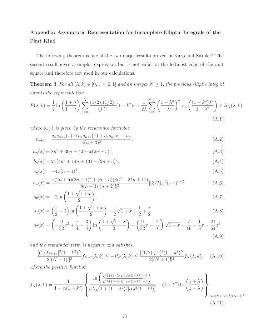
Appendix: Asymptotic Representation for Incomplete Elliptic Integrals of the

First Kind

The following theorem is one of the two major results proven in Karp and Sitnik.49 The

second result gives a simpler expression but is not valid on the leftmost edge of the unit

square and therefore not used in our calculations.

Theorem 3 For all (λ, k) ∈ [0, 1]× [0, 1] and an integer N ≥ 1, the previous elliptic integral

admits the representation

F (λ, k) =1

2ln

(

1 + λ

1− λ

) N∑

j=0

(1/2)j(1/2)j(j!)2

(1− k2)j +1

2λ

N−1∑

n=0

(

1− λ2

−λ2)n

sn

(

(1− k2)λ2

1− λ2

)

+RN (λ, k),

(A.1)

where sn(·) is given by the recurrence formulae

sn+3 =ansn+2(x),+bnsn+1(x) + cnsn(x) + hn

4(n+ 3)2, (A.2)

an(x) = 8n2 + 36n+ 42− x(2n+ 5)2, (A.3)

bn(x) = 2x(4n2 + 14n+ 13)− (2n+ 3)2, (A.4)

cn(x) = −4x(n + 1)2, (A.5)

hn(x) =x(2n + 5)(2n+ 4)2 + (n+ 3)(8n2 + 24n+ 17)

8(n+ 3)[(n+ 2)!]2[(3/2)n]

2(−x)n+2, (A.6)

s0(x) = −2 ln

(

1 +√1 + x

2

)

, (A.7)

s1(x) =(x

2− 1)

ln

(

1 +√1 + x

2

)

− 1

2

√1 + x+

1

2+x

2, (A.8)

s2(x) =

(

− 9

32x2 +

x

4− 3

4

)

ln

(

1 +√1 + x

2

)

+

(

9

32x− 7

16

)√1 + x+

7

16+

1

8x− 21

64x2

(A.9)

and the remainder term is negative and satisfies,

[(1/2)N+1]2(1− k2)N

2[(N + 1)!]2fN+1(λ, k) ≤ −RN (λ, k) ≤

[(1/2)N+1]2(1− k2)N

2[(N + 1)!]2fN (λ, k), (A.10)

where the positive function

fN(λ, k) =1

1− α(1− k2)

ln

(√1+(1−λ2)/[αλ2(1−k2)]+1√1+(1−λ2)/[αλ2(1−k2)]−1

)

αλ√

1 + (1− λ2)/[αλ2(1− k2)]− (1− k2) ln

(

1 + λ

1− λ

)

|α=(N+1/2)2/(N+1)2

(A.11)

13

is bounded on every subset of E of the unit square, where

supk,λ∈E

1− k

1− λ<∞ (A.12)

and is monotonically decreasing in N .

From this theorem we denote its first-order approximation as

F1(λ, k) = ln

(

√

1 + λ

1− λ

)

+1

λln

(

2

1 +√

(1− k2λ2)/(1− λ2)

)

+1− k2

8ln

(

1 + λ

1− λ

)

,

(A.13)

and note that this expression is asymptotic in the λ variable.

REFERENCES

1L. Landau, “Theory of the superfluidity of helium II,” Phys. Rev. 60, 356–358 (Aug 1941).

2L. D. Landau and E. M. Lifshitz, Course of Theoretical Physics: Fluid Mechanics (Oxford:

Pergamon Press, 1959).

3A. Griffin, “New light on the intriguing history of superfluidity in liquid 4He,” Journal of

Physics Condensed Matter 21, 164220–+ (Apr. 2009).

4R.P. Feynman, “Chapter II: Application of quantum mechanics to liquid helium,” (Else-

vier, 1955) pp. 17 – 53.

5L. Onsager, “Statistical hydrodynamics,” Il Nuovo Cimento (1943-1954) 6, 279–287 (1949).

6R. J. Donnelly, Quantized Vortices in Helium II (Cambridge University Press, 2005).

7C. F. Barenghi, “Introduction to Superfluid Vortices and Turbulence,” in

Quantized Vortex Dynamics and Superfluid Turbulence, Lecture Notes in Physics,

Berlin Springer Verlag, Vol. 571, edited by C. F. Barenghi, R. J. Donnelly, & W. F. Vinen

(2001) pp. 3–+.

8W. F. Vinen, “Mutual friction in a heat current in liquid helium II: I. Experiments on

steady heat currents,” Royal Society of London Proceedings Series A 240, 114–127 (Apr.

1957).

9W. F. Vinen, “Mutual friction in a heat current in liquid helium II: II. Experiments on

transient effects,” Royal Society of London Proceedings Series A 240, 128–143 (Apr. 1957).

10W. F. Vinen, “Mutual friction in a heat current in liquid helium II: III. Theory of the

mutual friction,” Royal Society of London Proceedings Series A 242, 493–515 (Nov. 1957).

14

11W. F. Vinen, “Mutual friction in a heat current in liquid helium II: IV. Critical heat

currents in wide channels,” Royal Society of London Proceedings Series A 243, 400–413

(Jan. 1958).

12K. W. Schwarz, “Theory of turbulence in superfluid 4he,” Physical Review Letters 38,

551–554 (Mar. 1977).

13K. W. Schwarz, “Three-dimensional vortex dynamics in superfluid 4he: Homogeneous

superfluid turbulence,” Physical Review B 38, 2398–2417 (Aug. 1988).

14D. C. Samuels, “Vortex Filament Methods for Superfluids,” in

Quantized Vortex Dynamics and Superfluid Turbulence, Lecture Notes in Physics,

Berlin Springer Verlag, Vol. 571, edited by C. F. Barenghi, R. J. Donnelly, & W. F. Vinen

(2001) pp. 97–+.

15E. A. L. Henn, J. A. Seman, G. Roati, K. M. F. Magalhaes, and V. S. Bagnato, “Emergence

of turbulence in an oscillating bose-einstein condensate,” Phys. Rev. Lett. 103, 045301 (Jul

2009).

16G. H. Cottet and J. Soler, “Three-dimensional navier-stokes equations for singular filament

initial data,” Journal of Differential Equations 74, 234 – 253 (1988).

17P. K. Newton, The N-Vortex Problem, Applied Mathematical Sciences, Vol. 145 (Springer,

2001).

18A. Leonard, “Vortex methods for flow simulation,” Journal of Computational Physics 37,

289–335 (Oct. 1980).

19A. Leonard, “Computing three-dimensional incompressible flows with vortex elements,”

Annual Review of Fluid Mechanics 17, 523–559 (1985).

20J. T. Beale and A. Majda, “Vortex methods. I - Convergence in three dimensions. II -

Higher order accuracy in two and three dimensions,” Mathematics of Computation 39,

1–52 (Jul. 1982).

21A. J. Chorin, “Vortex models and boundary layer instability,” SIAM Journal on Scientific

and Statistical Computing 1, 1–21 (1980).

22B. Couet, O Buneman, and A Leonard, “Simulation of three-dimensional incompressible

flows with a vortex-in-cell method,” Journal of Computational Physics 39, 305 – 328

(1981).

23W. T. Ashurst and E. Meiburg, “Three-dimensional shear layers via vortex dynamics,”

Journal of Fluid Mechanics 189, pp 87–116 ((1988)).

15

24R. L. Ricca, “Rediscovery of Da Rios equations,” Nature 352, 561–562 (Aug. 1991).

25R. Betchov, “On the curvature and torsion of an isolated vortex filament,” Journal of Fluid

Mechanics 22, 471–479 (1965).

26R. J. Arms and F. R. Hama, “Localized-Induction Concept on a Curved Vortex and Motion

of an Elliptic Vortex Ring,” Physics of Fluids 8, 553–559 (Apr. 1965).

27G. K. Batchelor, An Introduction to Fluid Dynamics (Cambridge University Press, 2000).

28A. J. Callegari and L. Ting, “Motion of a curved vortex filament with decaying vortical

core and axial velocity,” SIAM Journal of Applied Mathematics 35, 148–175 (Jul. 1978).

29R. L. Ricca, “The contributions of Da Rios and Levi-Civita to asymptotic potential theory

and vortex filament dynamics,” Fluid Dynamics Research 18, 245–268 (Oct. 1996).

30F. R. Hama, “Genesis of the LIA,” Fluid Dynamics Research 3, 149–150 (Sep. 1988).

31M. J. P. Cullen, “Vortex dynamics. Edited by P. G. Saffman. Cambridge University Press.

Pp. 31 1. Price 17.95 (paperback). ISBN 0 521 47739 5,” Quarterly Journal of the Royal

Meteorological Society 122, 1015–1015 (Apr. 1996).

32A. J. Majda and A. L. Bertozzi, Vorticity and Incompressible Flow (Cambridge University

Press, 2001).

33L.S. Da Rios, “Sul moto d’un liquido indefinito con un filetto vorticoso di forma qualunque

(on the motion of an unbounded liquid with a vortex filament of any shape),” Rend. Circ.

Mat. Palermo 22, 117135 (1906).

34L.S. Da Rios, “Sul moto dei filetti vorticosi di forma qualunque (on the motion of vortex

filaments of any shape),” Rend. R. Acc. Lincei 18, 7579 (1909).

35L.S. Da Rios, “Sul moto dei filetti vorticosi di forma qualunque (on the motion of vortex

filaments of any shape),” Rend. Circ. Mat. Palermo 29, 354368 (1910).

36L.S. Da Rios, “Sul moto intestino dei filetti vorticosi (on the interior motion of vortex

filaments),” Giornale di Matematiche del Battaglini 49, 300308 (1911).

37L.S. Da Rios, “Sezioni trasversali stabili dei filetti vorticosi (stable cross-sections of vortex

filaments),” Atti R. Ist. Veneto Sci. Lett. Arti 75, 299308 (1916).

38L.S. Da Rios, “Sui tubi vorticosi rettilinei posti a raffronto (comparative study of rectilinear

vortex tubes),” Atti R. Acc. Sci. Lett. Arti Padova 32, 343350 (1916).

39L.S. Da Rios, “Vortici ad elica (helical vortices),” II Nuovo Cimento 11, 419431 (1916).

40L.S. Da Rios, “Sur la thorie des tourbillons,” Comptes Rendus Acad. Sci. Paris 191,

399–401 (1930).

16

41L.S. Da Rios, “Sui vortici piani indeformabili (on planar vortices of invariant shape,” Atti

Pontificia Acc. Sci. Nuovi Lincei 84, 720–731 (1931).

42L.S. Da Rios, “Sui vortici piani indeformabili (on planar vortices of invariant shape),” Atti

Soc. Ital. Progresso Scienze 2, 7–8 (1931).

43L.S. Da Rios, “Anelli vorticosi ruotanti (rotating vortex rings),” Rend. Sem. Matem. Univ.

Padova 9, 142–151 (1931).

44L.S. Da Rios, “Ancora sugli anelli vorticosi ruotanti (again on rotating vortex rings),”

Rend. R. Acc. Lincei 17, 924–926 (1933).

45L.S. Da Rios, “Sui vortici gobbi indeformabili (on hunched vortices of invariant shape),”

Atti Pontificia Acc. Sci. Nuovi Lincei 86, 162–168 (1933).

46Y. Fukumoto and T. Miyazaki, “Three-dimensional distortions of a vortex filament with

axial velocity,” Journal of Fluid Mechanics 222, 369–416 (Jan. 1991).

47G. L. Lamb Jr., Elements of Soliton Theory, Vol. 4 (John Wiley and Sons, 1986) pp. 316–

+.

48K. W. Schwarz, “Generation of superfluid turbulence deduced from simple dynamical

rules,” Physical Review Letters 49, 283–285 (Jul. 1982).

49D. Karp and S. M. Sitnik, “Asymptotic approximations for the first incomplete elliptic

integral near logarithmic singularity,” Journal of Computational and Applied Mathematics

205, 186–206 (Aug. 2007).

50A. Erdelyi, Asymptotic Expansions (Dover, 1956).

51J. van der Corput, “Asymptotic developments I: Fundamental theorems of asymptotics,”

Journal d’Analyse Mathmatique 4, 341–418 (1954).

52J. van der Corput, “Asymptotic developments II: Generalization of the fundamental the-

orem on asymptotic series,” Journal d’Analyse Mathmatique 5, 315–320 (1956).

53J. van der Corput, “Asymptotic developments III: Again on the fundamental theorem of

asymptotic series,” Journal d’Analyse Mathmatique 9, 195–204 (1961).

54O. C. Idowu, A. Willis, C. F. Barenghi, and D. C. Samuels, “Local normal-fluid helium

II flow due to mutual friction interaction with the superfluid,” Physical Review B 62,

3409–3415 (Aug. 2000).

55O. C. Idowu, D. Kivotides, C. F. Barenghi, and D.C. Samuels, “Equation for self-consistent

superfluid vortex line dynamics,” Journal of Low Temperature Physics 120, 269–280

(2000).

17

56J. Kim and P. Moin, “Application of a fractional-step method to incompressible Navier-

Stokes equations,” Journal of Computational Physics 59, 308–323 (Jun. 1985).

57F. H. Harlow and J. E. Welch, “Numerical Calculation of Time-Dependent Viscous Incom-

pressible Flow of Fluid with Free Surface,” Physics of Fluids 8, 2182–2189 (Dec. 1965).

58A. A. Wray, “Very low storage time-advancement schemes,” (1986), internal Report, NASA

Ames Research Center, Moffet Field, California.

59C. A. Kennedy, M. H. Carpenter, and R. M. Lewis, “Low-storage, explicit runge-kutta

schemes for the compressible navier-stokes equations,” Applied Numerical Mathematics

35, 177 – 219 (2000).

60S. A. Ragab and K. S. Youssef, “Computational aspects of trailing vortices,” Journal of

Wind Engineering and Industrial Aerodynamics 69-71, 943 – 953 (1997).

61J. S. Hesthaven and T. Warburton, Nodal Discontinuous Galerkin Methods Algorithms, Analysis, and Applications

(Springer, 2008).

62L. Liu, X. Li, and F. Q. Hu, “Nonuniform time-step runge-kutta discontinuous galerkin

method for computational aeroacoustics,” Journal of Computational Physics 229, 6874–

6897 (Sep. 2010).

63T. F. Lemczyk and M. M. Yovanovich, “Efficient evaluation of incomplete elliptic integrals

and functions,” Computers & Mathematics with Applications 16, 747 – 757 (1988).

64W. C. Hassenpflug, “Elliptic integrals and the Schwarz-Christoffel transformation,” Com-

puters & Mathematics with Applications 33, 15–114 (JUN 1997).

65T. Fukushima and H. Ishizaki, “Numerical computation of incomplete elliptic integrals of

a general form,” Celestial Mechanics and Dynamical Astronomy 59, 237–251 (1994).

66X. Yang, “Efficient circular arc interpolation based on active tolerance control,” Computer-

Aided Design 34, 1037 – 1046 (2002).

67E. Hodby, G. Hechenblaikner, S. A. Hopkins, O. M. Marago, and C. J. Foot, “Vortex

nucleation in Bose-Einstein condensates in an oblate, purely magnetic potential,” Phys.

Rev. Lett. 88, 010405 (Dec 2001).

68E. Varoquaux, O. Avenel, Y. Mukharsky, and P. Hakonen, “The experimental evidence

for vortex nucleation in 4He,” in Quantized Vortex Dynamics and Superfluid Turbulence,

Lecture Notes in Physics, Berlin Springer Verlag, Vol. 571, edited by C. F. Barenghi,

R. J. Donnelly, & W. F. Vinen (2001) pp. 36–+.

18

69R. B. Pelz, “Locally self-similar, finite-time collapse in a high-symmetry vortex filament

model,” Physical Review E 55, 1617–1626 (Feb. 1997).

70J. Koplik and H. Levine, “Vortex reconnection in superfluid helium,” Physical Review

Letters 71, 1375–1378 (Aug. 1993).

71T. Lipniacki, “Evolution of quantum vortices following reconnection,” European Journal

of Mechanics B Fluids 19, 361–378 (May 2000).

72T. Lipniacki, “From Vortex Reconnections to Quantum Turbulence,” in

Quantized Vortex Dynamics and Superfluid Turbulence, Lecture Notes in Physics,

Berlin Springer Verlag, Vol. 571, edited by C. F. Barenghi, R. J. Donnelly, & W. F. Vinen

(2001) pp. 177–+.

73T. Lipniacki, “Evolution of the line-length density and anisotropy of quantum tangle in

4He,” Physical Review B 64, 214516–+ (Dec. 2001).

74D. Kivotides, C. F. Barenghi, and D. C. Samuels, “Superfluid vortex reconnections at finite

temperature,” Europhysics Letters 54, 774–778 (Jun. 2001).

75S. Gutierrez and L. Vega, “Self-similar solutions of the localized induction approximation:

singularity formation,” Nonlinearity 17, 2091–2136 (Nov. 2004).

76M. S. Paoletti, M. E. Fisher, and D. P. Lathrop, “Reconnection dynamics for quantized

vortices,” Physica D Nonlinear Phenomena 239, 1367–1377 (Jul. 2010).

77J. A. Seman, E. A. L. Henn, M. Haque, R. F. Shiozaki, E. R. F. Ramos, M. Caracanhas,

P. Castilho, C. Castelo Branco, P. E. S. Tavares, F. J. Poveda-Cuevas, G. Roati, K. M. F.

Magalhaes, and V. S. Bagnato, “Three-vortex configurations in trapped Bose-Einstein

condensates,” Physical Review A 82, 033616–+ (Sep. 2010).

78E. A. L. Henn, J. A. Seman, E. R. F. Ramos, M. Caracanhas, P. Castilho, E. P. Olımpio,

G. Roati, D. V. Magalhaes, K. M. F. Magalhaes, and V. S. Bagnato, “Observation of

vortex formation in an oscillating trapped Bose-Einstein condensate,” Phys. Rev. A 79,

043618 (Apr 2009).

79E. Henn, J. Seman, G. Roati, K. Magalhas, and V. Bagnato, “Generation of vortices and

observation of quantum turbulence in an oscillating Bose-Einstein condensate,” Journal of

Low Temperature Physics 158, 435–442 (2010).

80J. R. Abo-Shaeer, C. Raman, J. M. Vogels, and W. Ketterle, “Observation of Vortex

Lattices in Bose-Einstein Condensates,” Science 292, 476–479 (2001).

19

81K. W. Madison, F. Chevy, W. Wohlleben, and J. Dalibard, “Vortex formation in a stirred

bose-einstein condensate,” Phys. Rev. Lett. 84, 806–809 (Jan 2000).

82M. Kobayashi and M. Tsubota, “Quantum turbulence in a trapped Bose-Einstein conden-

sate under combined rotations around three axes,” Journal of Low Temperature Physics

150, 587–592 (2008).

83K. Kasamatsu, M. Tsubota, and M. Ueda, “Nonlinear dynamics of vortex lattice formation

in a rotating bose-einstein condensate,” Phys. Rev. A 67, 033610 (Mar 2003).

84Y. Castin and R. Dum, “Bose-einstein condensates in time dependent traps,” Phys. Rev.

Lett. 77, 5315–5319 (Dec 1996).

85H. E. Hall and W. F. Vinen, “The Rotation of Liquid Helium II. I. Experiments on the

Propagation of Second Sound in Uniformly Rotating Helium II,” Royal Society of London

Proceedings Series A 238, 204–214 (Dec. 1956).

86H. E. Hall and W. F. Vinen, “The Rotation of Liquid Helium II. II. The Theory of Mutual

Friction in Uniformly Rotating Helium II,” Royal Society of London Proceedings Series A

238, 215–234 (Dec. 1956).

87H. E. Hall, “The rotation of liquid helium II,” Advances in Physics 9, 89–146 (Jan. 1960).

88R. L. Ricca, “Tropicity and Complexity Measures for Vortex Tangles,” in

Quantized Vortex Dynamics and Superfluid Turbulence, Lecture Notes in Physics, Berlin

Springer Verlag, Vol. 571, edited by C. F. Barenghi, R. J. Donnelly, & W. F. Vinen (2001)

pp. 366–+.

89C. F Barenghi, R. L. Ricca, and D. C. Samuels, “How tangled is a tangle?.” Phys. D 157,

197–206 (2001).

90D. R. Poole, H. Scoffield, C. F. Barenghi, and D.C. Samuels, “Geometry and topology of

superfluid turbulence,” Journal of Low Temperature Physics 132, 97–117 (2003).

91D. Jou, M. S. Mongiovı, M. Sciacca, and C. F. Barenghi, “Vortex length, vortex energy and

fractal dimension of superfluid turbulence at very low temperature,” Journal of Physics

A: Mathematical and Theoretical 43, 205501 (2010).

92H. Hasimoto, “A soliton on a vortex filament,” Journal of Fluid Mechanics 51, 477–485

(1972).

93Annalisa Calini, “Recent developments in integrable curve dynamics,” (1997).

94P.G. Grinevich and M.U. Schmidt, “Closed curves in R3 : a characterization in terms of

curvature and torsion, the hasimoto map and periodic solutions of the filament equation..”.

20

95A. Calini and T. Ivey, “Finite-gap solutions tof the vortex filament equation: Genus one

solutions and symmetric solutions,” Journal of Nonlinear Science 15, 321–361 (2005).

96L. Uby, “Strings, Rods, Vortices and Wave Equations,” Royal Society of London Proceed-

ings Series A 452, 1531–1543 (Jul. 1996).

97R. L. Ricca, “Physical interpretation of certain invariants for vortex filament motion under

LIA,” Physics of Fluids 4, 938–944 (May 1992).

21