Density Difference Detection withApplication to Exploratory Visualization

Marko Rak, Tim Konig, Johannes Steffen, Dirk Joachim Lehmann, andKlaus-Dietz Tonnies

Department of Simulation and GraphicsOtto von Guericke University, Magdeburg, Germany

Abstract. Identifying differences among the distribution of samplesof different observations is an important issue in many research fields.We provide a general framework to detect these difference spots in d-dimensional feature space. Such spots occur not only at various loca-tions, they may also come in various shapes and multiple sizes, even atthe same location. We address these challenges by a scale-space repre-sentation of the density function difference of the observations in featurespace. Using three classification scenarios from UCI Machine LearningRepository we show that interest spots carry valuable information abouta data set. To this end, we establish a simple decision rule on top of ourframework. Results indicate state-of-the-art performance, underpinningthe importance of the information that is carried by the detected spots.Furthermore, we outline that the output of our framework can be usedto guide exploratory visualization of high-dimensional feature spaces.

Keywords: Density Difference, Kernel Density Estimation, Scale Space,Dendrogram, Blob Detection, Affine Shape Adaption, Exploratory Visu-alization, Orthographic Star Coordinates

1 Introduction

Sooner or later a large portion of pattern recognition tasks come down to thequestion What makes X different from Y ? Some scenarios of that kind are:

Detection of forged money based on image-derived features: What makessome sort of forgery different from genuine money?Comparison of medical data of healthy and non-healthy subjects fordisease detection: What makes the healthy different from the non-healthy?Comparison of document data sets for text retrieval purposes: Whatmakes this set of documents different from another set?

Apart from this, spotting differences in two or more observations is of interestin fields of computational biology, chemistry or physics. Looking at it from ageneral perspective, such questions generalize to

What makes samples of group X different from the samples of group Y ?

2 Rak et al.

This question usually arises when we deal with grouped samples in some featurespace. For humans, answering such questions tends to become more challengingwith increasing number of groups, samples and feature space dimensions, up tothe point where we miss the forest for the trees. This complexity is not an issueto automatic approaches, which, on the other hand, tend to either overfit orunderfit patterns in the data. Therefore, semi-automatic approaches are neededto generate a number of interest spots which are to be looked at in more detail.

We address this issue by a scale-space difference detection framework. Ourapproach relies on the density difference of group samples in feature space. Thisenables us to identify spots where one group dominates the other. We draw onkernel density estimators to represent arbitrary density functions. Embeddingthis into a scale-space representation, we are able to detect spots of differentsizes and shapes in feature space in an efficient manner. Our framework:

– applies to d-dimensional feature spaces– is able to reflect arbitrary density functions– selects optimal spot locations, sizes and shapes– is robust to outliers and measurement errors– produces human-interpretable results

Please note that large portions of the subsequent content were already cov-ered in our previous work [16]. Within the current work we go into detail on asecond spot detector (complementing the one used previously), provide an ex-tended evaluation and show how the output of our framework can be used toguide the exploratory visualization of high-dimensional feature spaces. The lat-ter may be seen as an intermediate step prior to applying other means of dataanalysis to the identified interest spots.

Our presentation is structured as follows. We outline the key foundations ofour framework in Section 2. The specific parts of our framework are detailed inSection 3, while Section 4 outlines our contribution to exploratory visualization.Section 5 comprises our results on several data sets from UCI Machine Learn-ing Repository. In Section 6, we close with a summary of our work, our mostimportant results and an outline of future work.

2 Theoretical Foundations

Searching for differences between the sample distribution of two groups of ob-servations g and h, we, quite naturally, seek for spots where the density functionfg(x) of group g dominates the density function fh(x) of group h, or vice versa.Hence, we try to find positive-/negative-valued spots of the density difference

fg−h(x) = fg(x)− fh(x) (1)

w.r.t. the underlying feature space Rd with x ∈ Rd. Such spots may come invarious shapes and sizes. A difference detection framework should be able todeal with these degrees of freedom. Additionally, it must be robust to varioussources of error, e.g. from measurement, quantization and outliers.

Density Difference Detection 3

We propose to superimpose a scale-space representation to the density dif-ference fg−h(x) to achieve the above-mentioned properties. Scale-space frame-works have been shown to robustly handle a wide range of detection tasks forvarious types of structures, e.g. text strings [23], persons and animals [8] innatural scenes, neuron membranes in electron microscopy imaging [20] or mi-croaneurysms in digital fundus images [2]. In each of these tasks the function ofinterest is represented through a grid of values, allowing for an explicit evaluationof the scale-space. However, an explicit grid-based approach becomes intractablefor higher-dimensional feature spaces.

In what follows, we show how a scale-space represenation of fg−h(x) can beobtained from kernel density estimates of fg(x) and fh(x) in an implicit fashion,expressing the problem by scale-space kernel density estimators. Note that bythe usage of kernel density estimates our work is limited to feature spaces withdense filling. We close with a brief discussion on how this can be used to compareobservations among more than two groups.

2.1 Scale Space Representation

First, we establish a family lg−h(x; t) of smoothed versions of the densitiy dif-ference lg−h(x). Scale parameter t ≥ 0 defines the amount of smoothing that isapplied to lg−h(x) via convolution with kernel kt(x) of bandwidth t as stated in

lg−h(x; t) = kt(x) ∗ fg−h(x). (2)

For a given scale t, spots having a size of about 2√t will be highlighted, while

smaller ones will be smoothed out. This leads to an efficient spot detectionscheme, which will be discussed in Section 3. Let

lg(x; t) = kt(x) ∗ fg(x) (3)

lh(x; t) = kt(x) ∗ fh(x) (4)

be the scale-space representations of the group densities fg(x) and fh(x). Look-ing at Equation 2 more closely, we can rewrite lg−h(x; t) equivalently in termsof lg(x; t) and lh(x; t) via Equation 3 and 4. This reads

lg−h(x; t) = kt(x) ∗ fg−h(x) (5)

= kt(x) ∗[fg(x)− fh(x)

](6)

= kt(x) ∗ fg(x)− kt(x) ∗ fh(x) (7)

= lg(x; t)− lh(x; t). (8)

The simple yet powerful relation between the left and the right-hand sideof Equation 8 will allow us to evaluate the scale-space representation lg−h(x)implicitly, i.e. using only kernel functions. Of major importance is the choice ofthe smoothing kernel kt(x). According to scale-space axioms, kt(x) should suffice

4 Rak et al.

a number of properties, resulting in the uniform Gaussian kernel of Equation 9as the unique choice, cf. [3, 24].

φt(x) =1√

(2πt)dexp

(− 1

2txTx

)(9)

2.2 Kernel Density Estimation

In kernel density estimation, the group density fg(x) is estimated from its ng

samples by means of a kernel function KBg (x). Let xgi ∈ Rd×1 with i = 1, . . . , ng

being the group samples. Then, the group density estimate is given by

fg(x) =1

ng

ng∑i=1

KBg (x− xgi ). (10)

Parameter Bg ∈ Rd×d is a symmetric positive-definite matrix, which controls thesample influence to the density estimate. Informally speaking, KBg (x) applies asmoothing with bandwidth Bg to the “spiky sample relief” in feature space.

Plugging kernel density estimator fg(x) into the scale-space representation

lg(x; t) defines the scale-space kernel density estimator lg(x; t) to be

lg(x; t) = kt(x) ∗ fg(x). (11)

Inserting Equation 10 into the above, we can trace down the definition of thescale-space density estimator lg(x; t) to the sample level via transformation

lg(x; t) = kt(x) ∗ fg(x) (12)

= kt(x) ∗

[1

ng

ng∑i=1

KBg (x− xgi )

](13)

=1

ng

ng∑i=1

(kt ∗KBg ) (x− xgi ). (14)

Though arbitrary kernels can be used, we choose KB(x) to be a Gaussiankernel ΦB(x) due to its convenient algebraic properties. This (potentially non-uniform) kernel is defined as

ΦB(x) =1√

det(2πB)exp

(−1

2xTB−1x

). (15)

Using the above, the right-hand side of Equation 14 simplifies further becauseof the Gaussian’s cascade convolution property. Eventually, the scale-space kerneldensity estimator lg(x; t) is given by Equation 16, where I ∈ Rd×d is the identity.

lg(x; t) =1

ng

ng∑i=1

ΦtI+Bg (x− xgi ) (16)

Density Difference Detection 5

Using this estimator, the scale-space representation lg(x; t) of group densityfg(x) and analogously that of group h can be estimated for any (x; t) in animplicit fashion. Consequently, this allows us to estimate the scale-space repre-sentation lg−h(x; t) of the density difference fg−h(x) via Equation 7 by meansof kernel functions only.

2.3 Bandwidth Selection

When regarding bandwidth selection in such a scale-space representation, we seethat the impact of different choices for bandwidth matrix B vanishes as scale tincreases. This can be seen when comparing matrices tI + 0 and tI + B where0 represents the zero matrix, i.e. no bandwidth selection at all. We observethat relative differences between them become neglectable once ‖tI‖ � ‖B‖.This is especially true for large sample sizes, because the bandwidth will thentend towards zero for any reasonable bandwidth selector anyway. Hence, we mayactually consider setting B to 0 for certain problems, as we typically search fordifferences that fall above some lower bound for t.

Literature bares extensive work on bandwidth matrix selection, for exam-ple, based on plug-in estimators [6, 21] or biased, unbiased and smoothed cross-validation estimators [7, 19]. All of these integrate well with our framework.However, in view of the argument above, we propose to compromise between afull bandwidth optimization and having no bandwidth at all. We define Bg = bgIand use an unbiased least-squares cross-validation to set up the bandwidth es-timate for group g. For Gaussian kernels, this leads to the optimization of 17,cf. [7], which we achieved by golden section search over bg.

arg minBg

1

ng√

det(4πBg)+

1

ng(ng − 1)

ng∑i=1

ng∑j=1j 6=i

(Φ2Bg − 2ΦBg ) (xgi − xgj ) (17)

2.4 Multiple Groups

If differences among more than two groups shall be detected, we can reduce thecomparison to a number of two-group problems. We can consider two typical usecases, namely one group vs. another and one group vs. rest. Which of the two ismore suitable depends on the specific task at hand. Let us illustrate this using twomedical scenarios. Assume we have a number of groups which represent patientshaving different diseases that are hard to discriminate in differential diagnosis.Then we may consider the second use case, to generate clues on markers thatmake one disease different from the others. In contrast, if these groups representstages of a disease, potentially including a healthy control group, then we mayconsider the first use case, comparing only subsequent stages to give clues onmarkers of the disease’s progress.

6 Rak et al.

3 Detection Framework

To identify the positve-/negative-valued spots of a density difference, we applythe concept of blob detection, which is well-known in computer vision, to thescale-space representation derived in Section 2. In scale-space blob detection,some blobness criterion is applied to the scale-space representation, seeking forlocal optima of the function of interest w.r.t. space and scale. This directly leadsto an efficient detection scheme that identifies a spot’s location and size. Thelatter corresponds to the detection scale.

In a grid-representable problem we can evaluate blobness densely over thescale-space grid and identify interesting spots directly using the grid neighbor-hood. This is intractable here, which is why we rely on a more refined three-stage approach. First, we trace the local spatial optima of the density differencethrough scales of the scale-space representation. Second, we identify the inter-esting spots by evaluating their blobness along the dendrogram of optima thatwas obtained during the first stage. Having selected spots and therefore knowingtheir locations and sizes, we finally calculate an elliptical shape estimate for eachspot in a third stage.

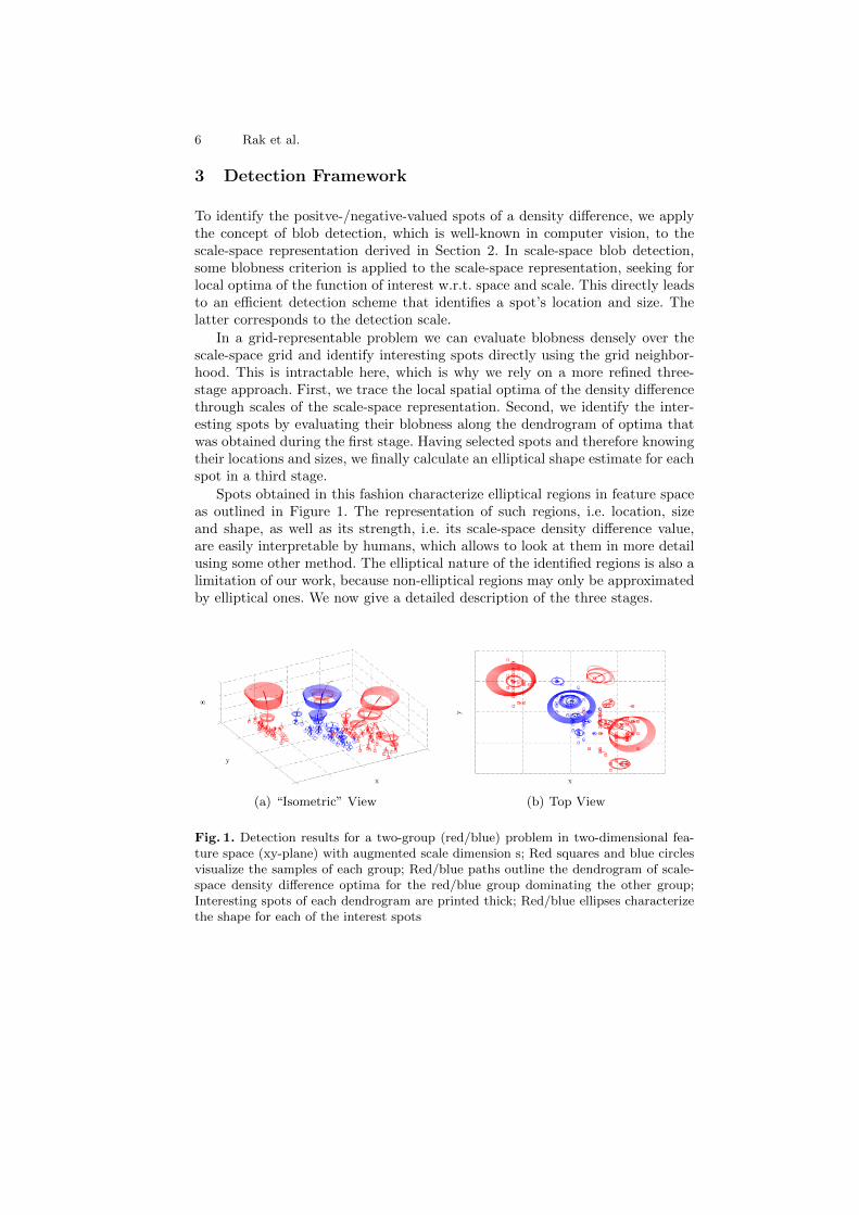
Spots obtained in this fashion characterize elliptical regions in feature spaceas outlined in Figure 1. The representation of such regions, i.e. location, sizeand shape, as well as its strength, i.e. its scale-space density difference value,are easily interpretable by humans, which allows to look at them in more detailusing some other method. The elliptical nature of the identified regions is also alimitation of our work, because non-elliptical regions may only be approximatedby elliptical ones. We now give a detailed description of the three stages.

(a) “Isometric” View (b) Top View

Fig. 1. Detection results for a two-group (red/blue) problem in two-dimensional fea-ture space (xy-plane) with augmented scale dimension s; Red squares and blue circlesvisualize the samples of each group; Red/blue paths outline the dendrogram of scale-space density difference optima for the red/blue group dominating the other group;Interesting spots of each dendrogram are printed thick; Red/blue ellipses characterizethe shape for each of the interest spots

Density Difference Detection 7

3.1 Scale Tracing

Assume we are given an equidistant scale sampling, containing non-negativescales t1, . . . , tn in increasing order and we search for spots where group g dom-inates h. More precisely, we search for the non-negatively valued maxima oflg−h(x; ti−1). The opposite case, i.e. group h dominates g, is equivalent.

Let us further assume that we know the spatial local maxima of the densitydifference lg−h(x; ti−1) for a certain scale ti−1 and we want to estimate thoseof the current scale ti. This can be done taking the previous local maxima asinitial points and optimizing each w.r.t. lg−h(x; ti). In the first scale, we take thesamples of group g themselves. As some maxima may be converged to the samelocation, we merge them together, feeding unique locations as initials into thenext scale ti+1 only. We also drop any negatively-valued locations as these arenot of interest to our task. They will not become of interest for any higher scaleeither, because local extrema will not enhance as scale increases, cf. [13]. Sincederivatives are simple to evaluate for Gaussian kernels, we can use Newton’smethod for spatial optimization. We can assemble gradient ∂

∂x lg−h(x; t) and

Hessian ∂2

∂x∂xT lg−h(x; t) sample-wise using

∂

∂xΦB(x) = −ΦB(x) B−1x and (18)

∂2

∂x∂xTΦB(x) = ΦB(x)

(B−1xxTB−1 −B−1

). (19)

Iterating this process through all scales, we form a discret dendrogram ofthe maxima over scales. A dendrogram branching means that a maxima formedfrom two (or more) maxima from the preceding scale.

3.2 Spot Detection

The maxima of interest are derived from a scale-normalized blobness criterioncγ(x; t). Two main criteria, namely the determinant of the Hessian [5] given inEquation 201 and the trace of the Hessian [13] given in Equation 22 have beendiscussed in literature. In contrast to our previous work [16], we do not focus ona single criterion. Instead, we will later investigate both in comparison.

cdetγ (x; t) = tγd (−1)ddet

(∂2

∂x∂xTlg−h(x; t)

)︸ ︷︷ ︸ (20)

= tγd cdet(x; t) (21)

ctrγ (x; t) = tγd (−1)tr

(∂2

∂x∂xTlg−h(x; t)

)︸ ︷︷ ︸ (22)

= tγd ctr(x; t) (23)

1 (−1)d leads to a consistent criterion for even and odd dimensions.

8 Rak et al.

Because the maxima are already spatially optimal, we can search for spots thatmaximize cγ(x; t) w.r.t. the dendrogram neighborhood only. Note that we donot require the superscript because the remained is independent of the choiceof the blobness criterion. Parameter γ ≥ 0 can be used to introduce a size bias,shifting the detected spot towards smaller or larger scales. The definition of γhighly depends on the type of spot that we are looking for, cf. [12]. This isimpractical when we seek for spots of, for example, small and large skewness orextreme kurtosis at the same time.

Addressing the parameter issue, we search for all spots that maximize cγ(x; t)locally w.r.t. some γ ∈ [0,∞). Some dendrogram spot s with scale-space coordi-nates (xs; ts) is locally maximal if there exists a γ-interval such that its blobnesscγ(xs; ts) is larger than that of every spot in its dendrogram neighborhood N (s).This leads to a number of inequalities, which can be written as

tγds c(xs; ts) >∀n∈N (s)

tγdn c(xn; tn) or (24)

γ d logtstn

>∀n∈N (s)

logc(xn; tn)

c(xs; ts). (25)

The latter can be solved easily for the γ-interval, if any. We can now identifyour interest spots by looking for the maxima along the dendrogram that locallymaximize the width of the γ-interval. More precisely, let wγ(xs; ts) be the widthof the γ-interval for dendrogram spot s, then s is of interest if the dendrogramLaplacian of wγ(x; t) is negative at (xs; ts), or equivalently, if

wγ(xs; ts) >1

|N (s)|∑

n∈N (s)

wγ(xn; tn). (26)

Intuitively, a spot is of interest if its γ-interval width is above neighborhoodaverage. This is the only assumption we can make without imposing limitationson the results. Interest spots indentified in this way will be dendrogram segments,each ranging over a number of consecutive scales.

3.3 Shape Adaption

Shape estimation can be done in an iterative manner for each interest spot. Theiteration alternatingly updates the current shape estimate based on a measure ofanisotropy around the spot and then corrects the bandwidth of the scale-spacesmoothing kernel according to this estimate, eventually reaching a fixed point.The second moment matrix of the function of interest is typically used as ananisotropy measure, e.g. in [14] and [15]. Since it requires spatial integrationof the scale-space representation around the interest spot, this measure is notfeasible here.

We adapted the Hessian-based approach of [10] to d-dimensional problems.The aim is to make the scale-space representation isotropic around the inter-est spot, iteratively moving any anisotropy into the symmetric positive-definite

Density Difference Detection 9

shape matrix S ∈ Rd×d of the smoothing kernel’s bandwidth tS. Thus, we lift theproblem into a generalized representation lg−h(x; tS) of anisotropic scale-spacekernels, which requires us to replace the definition of φt(x) by that of ΦB(x).

Starting with the isotropic S1 = I, we decompose the current Hessian via

∂2

∂x∂xTlg−h( · ; tSi) = VD2VT (27)

into its eigenvectors in columns of V and eigenvalues on the diagonal of D2. Wethen normalize the latter to unit determinant via

D = d√

det(D)D (28)

to get a relative measure of anisotropy for each of the eigenvector directions.Finally, we move the anisotropy into the shape estimate via

Si+1 =(VTD−

12 V)

Si

(VD−

12 VT

)(29)

and start all over again. Iteration terminates when isotropy is reached. Moreprecisely: when the ratio of minimal and maximal eigenvalue of the Hessianapproaches one, which usually happens within a few iterations.

4 Exploratory Visualization

As mentioned introductory, exploratory visualization may be a reasonable in-termediate step prior to directly applying other means of data analysis to theinterest spots. There are plenty of visualization techniques that aim at identifi-cation of interesting patterns in the distribution of samples in high-dimensionalfeature spaces. For this work, we focus on a recent in-house development namelyorthographic star coordinates [11]. We next give a short introduction to thetopic and discuss how outputs of our framework can be used to guide the visualexploration process.

4.1 Star Coordinate Visualization

Star coordinate visualizations make use of projections from d-dimensional fea-ture spaces to a two-dimensional projection plane which is then visualized. Suchprojections are characterized by a projection matrix P ∈ R2×d the columns ofwhich can be interpreted as d points in two-dimensional space. Modifying theseso-called anchor points is equivalent to manipulation of the projection plane it-self, which the star coordinate visualization exploits by an interactive interfacelike that shown in Figure 2.

In general, star coordinates allow for arbitrary projections thus potentiallyintroducing arbitrary distortions to the visualization of the high-dimensionalcontent. This is not desirable for various reasons, therefore [11] proposed to re-strict the interaction to orthographic projections. Orthography is directly related

10 Rak et al.

12

3

4

(a) Original View

12

3

4

(b) Augmented View

1

23

4

(c) Focused View

Fig. 2. Exploratory visualization of a three-group (red/green/blue) problem in 4-dimensional feature space by orthographic star coordinates; Original orthographic starcoordinates (left) augmented with output of our framework (middle) and focused on aparticular interest spot (right); Moveable anchor points are connected to the origin bythick black line segments; A slider for scale selection is located at the bottom of theinterface; The remaining visual content is discussed in the text

to d-dimensional rotation, enforcing this property thus provides an intuitive wayto “rotate” the high-dimensional content in front of a user’s viewpoint. This di-rectly targets the human’s ability to interpret spatial relations from a steerablesequence of projections which is pretty much what we do with two-dimensionalvisualizations of three-dimensional content on a daily basis.

4.2 Preserving Orthography

Regarding orthography, we have to address two main issues. First, how to recoveran orthographic projection when starting from an arbitrary projection. Second,how to reinforce orthography during interactive anchor movement. A sufficientcondition for orthography of some anchor point constellation Po ∈ R2×d is that

PoPoT = I, (30)

whereby I ∈ R2×2 is the identity matrix, cf. [11]. Therefore, given an arbitrarynon-orthographic P we may seek to make PPT ∈ R2×2 identity. Since the latterGramian matrix is almost certainly positive-definite in practice,2 we can obtainit’s Cholesky factor L ∈ R2×2 and manipulate the decomposition as follows

LLT = PPT (31)

I = L−1P︸ ︷︷ ︸PTL−T︸ ︷︷ ︸ (32)

I = Po PoT (33)

2 Rare semi-definite cases are avoided by regularization PPT + εI for some small ε.

Density Difference Detection 11

with Po being the recovered orthographic projection.3 Regarding the second is-sue, we can simply take the steps just outlined, continuously reinforcing orthog-raphy during interactive movement of particular anchors. Note how the anchorpoints of the given non-orthographic P are all transformed in the same man-ner by the (inverse of the) Cholesky factor L to obtain the orthographic anchorpoints Po. This avoids any experience of “arbitrariness” during user interaction.

4.3 Guiding Explorations

As already discussed in [11], there are certain open questions associated to starcoordinate visualizations. This includes suitable anchor point constellations, cen-ters of “rotation”, i.e. the choice of the origin in d-dimensional feature space priorto projection, as well as a reasonable zoom into the data after projection. Other-wise put, we need to know where to look at and how. The interest spots detectedby our framework can be used to address these issues, thereby also providing aninteractive mechanism to switch among potentially interesting structures.

As show in Figure 2, we have augmented the star coordinate visualization bya scale selection slider, letting the user choose the size (scale) of structures he/sheis interested in. Based on his/her selection, the visualization is overlayed withthe output of our framework that corresponds to the selected scale. Specifically,we transparently visualize the locations of maxima that were found during scaletracing (see Section 3.1) and their respective shapes, which were estimated duringshape adaption (see Section 3.3). In case a maximum was found interesting (seeSection 3.2), it’s location and shape is highlighted opaquely instead.

When interactively selecting a maxima, the visualization is changed to putfocus on the selection. Specifically, the origin of the d-dimensional feature spaceis shifted to the maxima’s location thereby making it the center of “rotation”.The user can then change the zoom to a multiple of the maxima’s scale bykeyboard bindings if desired. By another binding, he/she may also align theprojection plane with the two most significant axes of the shape estimate toget a reasonable initial constellation of anchor points. To this end, the uniteigenvectors that correspond to the two largest eigenvalues of the shape estimateare used to fill the rows of the projection matrix.

We combined the above with a binding that resets the visualization to justbefore focusing a selection which allows to rapidly explore several potentiallyinteresting spots before the user eventually moves on to differently sized struc-tures. Changing the scale selection slider steadily, the course of locations andshapes of the maxima gives an impression on how the data is structured fromcoarse to fine without missing any highlighted interest spot.

5 Experiments

We next demonstrate that interest spots carry valuable information about a dataset. Due to the lack of data sets that match our particular detection task a ground

3 This formulation is another view on the Gram-Schmidt process used in [11].

12 Rak et al.

truth comparison is impossible. Certainly, artificially constructed problems arean exception. However, the generalizability of results is at least questionable forsuch problems. Therefore, we chose to benchmark our approach indirectly via anumber of classification tasks. The rational is that results that are comparableto those of well-established classifiers should underpin the importance of theidentified interest spots.

Next we show how to use these interest spots for classification using a sim-ple decision rule and detail the data sets that were used. We then investigateparameters of our approach and discuss the results of the classification tasksin comparison to decision trees, Fisher’s linear discriminant analysis, k-nearestneighbors with optimized k and support vector machines with linear and cubickernels. All experiments were performed via leave-one-out cross-validation.

5.1 Decision Rule

To perform classification we establish a simple decision rule based on interestspots that were detected using the one group vs. rest use case. Therefore, wedefine a group likelihood criterion as follows. For each group g, having the setof interest spots Ig, we define

pg(x) = maxs∈Ig

lg−h (xs; tsSs) · exp

(−1

2(x− xs)

T(tsSs)

−1(x− xs)

). (34)

This is a quite natural trade-off, where the first factor favors spots s with highdensity difference, while the latter factor favors spots with small Mahalanobisdistance to the location x that is investigated. We may also think of pg(x) as anexponential approximation of the scale-space density difference using interestingspots only. Given this, our decision rule simply takes the group that maximizesthe group likelihood for the location of interest x. Figure 3 illustrate the decisionboundary obtained from this rule.

5.2 Data Sets

We carried out our experiments on three classification data sets taken from UCIMachine Learning Repository. A brief summary of them is given in Table 1. Inthe first task, we distinguish between benign and malign breast cancer based onmanually graded cytological charateristics, cf. [22]. In the second task, we dis-tinguish between genuine and forged money based on wavelet-transform-derivedfeatures from photographs of banknote-like specimen, cf. [9]. In the third task,we differentiate among normal, spondylolisthetic and disc-herniated vertebralcolumns based on biomechanical attributes derived from shape and orientationof the pelvis and the lumbar vertebral column, cf. [4].

5.3 Parameter Investigation

Before detailing classification results, we investigate two aspects of our approach.Firstly, we inspect the importance of bandwidth selection, benchmarking no

Density Difference Detection 13

(a) “Isometric” View (b) Top View

Fig. 3. Feature space decision boundaries (black plane curves) obtained from grouplikelihood criterion for the two-dimensional two-group problem of Figure 1 using cdetγ

for spot detection; Red squares and blue circles visualize the samples of each group;Red/blue paths outline the dendrogram of scale-space density difference optima for thered/blue group dominating the other group; Interesting spots of each dendrogram areprinted thick; Red/blue ellipses characterize the shape for each of the interest spots

Table 1. Data sets from UCI Machine Learning Repository

Breast Cancer Banknote Authentication Vertebral Column

Groups benign/malign genuine/forged normal/spondylo./herniatedSamples 444/239 762/610 100/150/60

Dimensions 10 4 6

kernel density bandwidth against the least-squares cross-validation techniquethat we use. Secondly, we determine the influence of the scale sampling rate. Forthe latter we space n+ 1 scales for various n equidistantly from zero to

tn = F−1χ2 (1− ε|d) maxg

(d

√det (Σg)

), (35)

where F−1χ2 ( · |d) is the cumulative inverse-χ2 distribution with d degrees of free-dom and Σg is the covariance matrix of group g. Intuitively, tn captures theextent of the group with largest variance up to a small ε, i.e. here 1.5 · 10−8.

To investigate the two aspects, we compare classification accuracies with andwithout bandwidth selection as well as sampling rates ranging from n = 100 ton = 300 in steps of 25. From the results, which are given in Table 2, we observethat bandwidth selection is almost neglectable for the Breast Cancer (BC) andthe Banknote Authentication (BA) data set no matter which criterion is used forspot detection. However, the impact is substantial throughout all scale samplingrates for the Vertebral Column (VC) data set for both criteria. This may be dueto the comparably small number of samples per group for this data set.

Regarding the second aspect, we observe that for both criteria the BA andVC data set classification accuracy increases only slightly when the scale sam-pling rate rises. On the BC data set, accuracy remains stable, except for thelower rates when cdetγ is used for spot detection. There is no such drop for the

14 Rak et al.

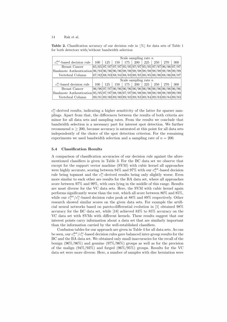
Table 2. Classification accuracy of our decision rule in b%c for data sets of Table 1for both detectors with/without bandwidth selection

Scale sampling rate n

cdetγ -based decision rule 100 125 150 175 200 225 250 270 300

Breast Cancer 65/65 97/97 97/97 95/95 97/97 95/95 97/97 96/96 97/97Banknote Authentication 96/94 96/96 96/96 98/98 98/98 98/98 98/98 98/98 99/99

Vertebral Column 87/82 88/83 88/84 88/83 88/85 88/85 88/86 88/86 88/87

Scale sampling rate nctrγ -based decision rule 100 125 150 175 200 225 250 270 300

Breast Cancer 96/96 97/97 96/96 96/96 96/96 96/96 96/96 96/96 96/96Banknote Authentication 95/95 97/97 98/98 97/97 98/98 98/98 98/98 98/99 99/99

Vertebral Column 89/81 89/80 89/80 89/83 89/83 89/84 89/83 89/84 89/83

ctrγ -derived results, indicating a higher sensitivity of the latter for sparser sam-plings. Apart from that, the differences between the results of both criteria areminor for all data sets and sampling rates. From the results we conclude thatbandwidth selection is a necessary part for interest spot detection. We furtherrecommend n ≥ 200, because accuracy is saturated at this point for all data setsindependently of the choice of the spot detection criterion. For the remainingexperiments we used bandwidth selection and a sampling rate of n = 200.

5.4 Classification Results

A comparison of classification accuracies of our decision rule against the afore-mentioned classifiers is given in Table 3. For the BC data set we observe thatexcept for the support vector machine (SVM) with cubic kernel all approacheswere highly accurate, scoring between 94% and 97% with our cdetγ -based decisionrule being topmost and the ctrγ -derived results being only slightly worse. Evenmore similar to each other are results for the BA data set, where all approachesscore between 97% and 99%, with ours lying in the middle of this range. Resultsare most diverse for the VC data sets. Here, the SVM with cubic kernel againperforms significantly worse than the rest, which all score between 80% and 85%,while our cdetγ /ctrγ -based decision rules peak at 88% and 89% respectively. Otherresearch showed similar scores on the given data sets. For example the artifi-cial neural networks based on pareto-differential evolution in [1] obtained 98%accuracy for the BC data set, while [18] achieved 83% to 85% accuracy on theVC data set with SVMs with different kernels. These results suggest that ourinterest points carry information about a data set that are similarly importantthan the information carried by the well-established classifiers.

Confusion tables for our approach are given in Table 4 for all data sets. As canbe seen, our cdetγ /ctrγ -based decision rules gave balanced inter-group results for theBC and the BA data set. We obtained only small inaccuracies for the recall of thebenign (96%/96%) and genuine (97%/96%) groups as well as for the precisionof the malign (94%/93%) and forged (96%/95%) groups. Results for the VCdata set were more diverse. Here, a number of samples with disc herniation were

Density Difference Detection 15

Table 3. Classification accuracies of different classifiers in b%c for data sets of Table 1

Breast Cancer Banknote Authen. Verteral Column

decision tree 94 98 82k-nearest neighbors 97 99 80

Fisher’s discriminant 96 97 80linear/cubic kernel SVM 96/90 99/98 85/74

cdetγ /ctrγ -based decision rule 97/96 98/98 88/89

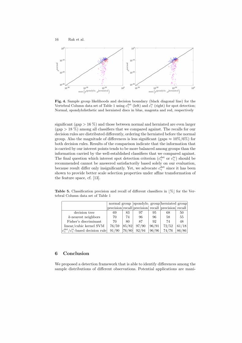
mistaken for being normal, lowering the recall of the herniated group (86%/86%)noticeably. However, more severe inter-group imbalances were caused by thenormal samples, which were relatively often mistaken for being spondylolistheticor herniated discs. Thus, recall for the normal group (76%/80%) and precisionfor the herniated group (74%/76%) decreased significantly. The latter is to somedegree caused by a handful of strong outliers from the normal group that fall intoeither of the other groups, which can already be seen from the group likelihoodplots in Figure 4. This finding was made by others as well, cf. [17].

Table 4. Confusion table for predicted/actual groups of our cdetγ /ctrγ -based decisionrule for data sets of Table 1

(a) Breast Cancer

HHHHHpred.

act.benign malign precision

benign 429/429 4/6 99/98malign 15/15 235/233 94/93

recall 96/96 98/97 b%c

(b) Banknote Authentication

HHHHHpred.

act.genuine forged precision

genuine 742/736 0/0 100/100forged 20/26 610/610 96/95

recall 97/96 100/100 b%c

(c) Vertebral Column

HHHHHpred.act.

normal spondylo. herniated precision

normal 76/80 1/1 6/7 91/90spondylo. 10/8 145/145 2/1 92/94herniated 14/12 4/4 52/52 74/76

recall 76/80 96/96 86/86 b%c

The other classifiers performed similarly balanced on the BA and BC data set.Major differences occured on the VC data set only. A precision/recall comparisonof all classifiers on the VC data set is given in Table 5. We observe that theprecision of the normal and the herniated group are significantly lower (gap >12%) than that of the spondylolisthetic group for all classifiers except for ourdecision rules, for which at least the normal group is predicted with a similarprecision by both rules. Regarding the recall we note an even more unbalancedbehavior. Here, a strict ordering from spondylolisthetic over normal to herniateddisks occurs. The differences of the recall of spondylolisthetic and normal are

16 Rak et al.

max(

pspondylo.

, pherniated

)

10-30 10-20 10-10 100

pnorm

al

10-30

10-20

10-10

100

max(

pspondylo.

, pherniated

)

10-30 10-20 10-10 100

pnorm

al

10-30

10-20

10-10

100

Fig. 4. Sample group likelihoods and decision boundary (black diagonal line) for theVertebral Column data set of Table 1 using cdetγ (left) and ctrγ (right) for spot detection;Normal, spondylolisthetic and herniated discs in blue, magenta and red, respectively

significant (gap > 16 %) and those between normal and herniated are even larger(gap > 18 %) among all classifiers that we compared against. The recalls for ourdecision rules are distributed differently, ordering the herniated before the normalgroup. Also the magnitude of differences is less significant (gaps ≈ 10%/6%) forboth decision rules. Results of the comparison indicate that the information thatis carried by our interest points tends to be more balanced among groups than theinformation carried by the well-established classifiers that we compared against.The final question which interest spot detection criterion (cdetγ or ctrγ ) should berecommended cannot be answered satisfactorily based solely on our evaluation,because result differ only insignificantly. Yet, we advocate cdetγ since it has beenshown to provide better scale selection properties under affine transformation ofthe feature space, cf. [13].

Table 5. Classification precision and recall of different classifiers in b%c for the Ver-tebral Column data set of Table 1

normal group spondylo. group herniated groupprecision recall precision recall precision recall

decision tree 69 83 97 95 68 50k-nearest neighbors 70 74 96 96 58 55

Fisher’s discriminant 70 80 87 92 74 48linear/cubic kernel SVM 76/59 85/82 97/90 96/91 72/52 61/18

cdetγ /ctrγ -based decision rule 91/90 76/80 92/94 96/96 74/76 86/86

6 Conclusion

We proposed a detection framework that is able to identify differences among thesample distributions of different observations. Potential applications are mani-

Density Difference Detection 17

fold, touching fields such as medicine, biology, chemistry and physics. Our ap-proach bases on the density function difference of the observations in featurespace, seeking to identify spots where one observation dominates the other. Su-perimposing a scale-space framework to the density difference, we are able todetect interest spots of various locations, size and shapes in an efficient manner.

Our framework is intended for semi-automatic processing, providing human-interpretable interest spots for further investigation of some kind. We outlinedhow the output of our framework can be used to guide exploratory visualizationof high-dimensional feature spaces as an intermediate step prior to other meansof data analysis. Furthermore, we showed that the detected interest spots carryvaluable information about a data set on a number of classification tasks from theUCI Machine Learning Repository. To this end, we established a simple decisionrule on top of our framework. Results indicate state-of-the-art performance ofour approach, which underpins the importance of the information that is carriedby the detected interest spots.

In the future, we plan to extend our work to support repetitive features suchas angles, which currently is a limitation of our approach. Modifying our notionof distance, we would then be able to cope with problems defined on, e.g. asphere or torus. Future work may also include the migration of other types ofscale-space detectors to density difference problems. This includes the notion ofridges, valleys and zero-crossings, leading to richer sources of information.

Acknowledgements This research was partially funded by the project “VisualAnalytics in Public Health” (TO 166/13-2) of the German Research Foundation.

References

1. Abbass, H.A.: An evolutionary artificial neural networks approach for breast cancerdiagnosis. Artificial Intelligence in Medicine 25, 265–281 (2002)

2. Adal, K.M., Sidibe, D., Ali, S., Chaum, E., Karnowski, T.P., Meriaudeau, F.:Automated detection of microaneurysms using scale-adapted blob analysis andsemi-supervised learning. Computer Methods and Programs in Biomedicine 114,1–10 (2014)

3. Babaud, J., Witkin, A.P., Baudin, M., Duda, R.O.: Uniqueness of the Gaussian ker-nel for scale-space filtering. IEEE Transactions on Pattern Analysis and MachineIntelligence 8, 26–33 (1986)

4. Berthonnaud, E., Dimnet, J., Roussouly, P., Labelle, H.: Analysis of the sagittalbalance of the spine and pelvis using shape and orientation parameters. Journal ofSpinal Disorders and Techniques 18, 40–47 (2005)

5. Bretzner, L., Lindeberg, T.: Feature tracking with automatic selection of spatialscales. Computer Vision and Image Understanding 71, 385–392 (1998)

6. Duong, T., Hazelton, M.L.: Plug-in bandwidth matrices for bivariate kernel densityestimation. Journal of Nonparametric Statistics 15, 17–30 (2003)

7. Duong, T., Hazelton, M.L.: Cross-validation bandwidth matrices for multivariatekernel density estimation. Scandinavian Journal of Statistics 32, 485–506 (2005)

18 Rak et al.

8. Felzenszwalb, P.F., Girshick, R.B., McAllester, D., Ramanan, D.: Object detectionwith discriminatively trained part-based models. IEEE Transactions on PatternAnalysis and Machine Intelligence 32, 1627–1645 (2010)

9. Glock, S., Gillich, E., Schaede, J., Lohweg, V.: Feature extraction algorithm forbanknote textures based on incomplete shift invariant wavelet packet transform.In: Annual Pattern Recognition Symposium. vol. 5748, pp. 422–431 (2009)

10. Lakemond, R., Sridharan, S., Fookes, C.: Hessian-based affine adaptation of salientlocal image features. Journal of Mathematical Imaging and Vision 44, 150–167(2012)

11. Lehmann, D.J., Theisel, H.: Orthographic star coordinates. IEEE Transactions onVisualization and Computer Graphics 19, 2615–2624 (2013)

12. Lindeberg, T.: Edge detection and ridge detection with automatic scale selection.In: IEEE Computer Society Conference on Computer Vision and Pattern Recog-nition. pp. 465–470 (1996)

13. Lindeberg, T.: Feature detection with automatic scale selection. International Jour-nal of Computer Vision 30, 79–116 (1998)

14. Lindeberg, T., Garding, J.: Shape-adapted smoothing in estimation of 3-d depthcues from affine distortions of local 2-d brightness structure. In: European Confer-ence on Computer Vision. pp. 389–400 (1994)

15. Mikolajczyk, K., Schmid, C.: Scale & affine invariant interest point detectors. In-ternational Journal of Computer Vision 60, 63–86 (2004)

16. Rak, M., Konig, T., Tonnies, K.D.: Spotting differences among observations. In:International Conference on Pattern Recognition Applications and Methods. pp.5–13 (2015)

17. Rocha Neto, A.R., Barreto, G.A.: On the application of ensembles of classifiers tothe diagnosis of pathologies of the vertebral column: A comparative analysis. IEEELatin America Transactions 7, 487–496 (2009)

18. Rocha Neto, A.R., Sousa, R., Barreto, G.A., Cardoso, J.S.: Diagnostic of pathologyon the vertebral column with embedded reject option. In: Pattern Recognition andImage Analysis, vol. 6669, pp. 588–595. Springer Berlin Heidelberg (2011)

19. Sain, S.R., Baggerly, K.A., Scott, D.W.: Cross-validation of multivariate densities.Journal of the American Statistical Association 89, 807–817 (1992)

20. Seyedhosseini, M., Kumar, R., Jurrus, E., Giuly, R., Ellisman, M., Pfister, H.,Tasdizen, T.: Detection of neuron membranes in electron microscopy images usingmulti-scale context and Radon-like features. In: International Conference on Med-ical Image Computing and Computer-assisted Intervention. pp. 670–677 (2011)

21. Wand, M.P., Jones, M.C.: Multivariate plug-in bandwidth selection. Computa-tional Statistics 9, 97–116 (1994)

22. Wolberg, W., Mangasarian, O.: Multisurface method of pattern separation for med-ical diagnosis applied to breast cytology. In: National Academy of Sciences. pp.9193–9196 (1990)

23. Yi, C., Tian, Y.: Text string detection from natural scenes by structure-basedpartition and grouping. IEEE Transactions on Image Processing 20, 2594–2605(2011)

24. Yuille, A.L., Poggio, T.A.: Scaling theorems for zero crossings. IEEE Transactionson Pattern Analysis and Machine Intelligence 8, 15–25 (1986)