demand systems and fresh vegetables: an ...afcerc.tamu.edu/publications/publication-pdfs/cp 1...

DEMAND SYSTEMS AND FRESH VEGETABLES: AN APPLICATION OF THE BARTEN APPROACH

Jaime E. Málaga Gary W. Williams

TAMRC Information Report CP 1-00March 2000


Texas Agricultural Market Research Center (TAMRC) Information Report No. CP 1-00, by Dr.Jaime Málaga and Dr. Gary Williams, Department of Agricultural Economics, Texas A&MUniversity, College Station, Texas, March 2000.

Abstract: The Barten approach is used to select the demand system specification for U.S. andMexican fresh vegetable demands. The Rotterdam model was found the most appropriateformulation for U.S. and Mexican demand systems, both in winter and summer. Onion demand wasfound weakly separable from the other fresh vegetable demands.

Key Words: fresh vegetables, demand systems

The Texas Agricultural Market Research Center (TAMRC) has been providing timely, unique,and professional research on a wide range of issues relating to agricultural markets andcommodities of importance to Texas and the nation for nearly thirty years. TAMRC is a marketresearch service of the Texas Agricultural Experiment Station and the Texas Agricultural ExtensionService. The main TAMRC objective is to conduct research leading to expanded and more efficientmarkets for Texas and U.S. agricultural products. Major TAMRC research divisions includeInternational Market Research, Consumer and Product Market Research, Commodity MarketResearch, and Contemporary Market Issues Research.


Executive Summary

Growing produce imports from Mexico and rapid gains in production efficiencies have kept U.S.fresh vegetable prices declining in real terms in recent years. Accuracy in the measurement of freshvegetable demand parameters in both the U.S. and Mexico is key to evaluating the futureprofitability of the U.S. fresh vegetable industry in the context of a North American free trade area.Only two serious attempts (Mittelhammer 1978 and Scott 1991) have been made to use demandsystems to estimate the parameters for U.S. fresh vegetable demand. In both cases, however, theselection of the demand system was arbitrary.

An important structural characteristic of the fresh vegetable markets in the U.S. and Mexico is theseasonality of production and trade. At least two clearly different U.S. and Mexicanproduction/marketing seasons exist (winter or fall-winter and spring-summer). Nevertheless, giventhe strong competition between the U.S. and Mexico during the winter season, most fresh vegetablequantitative analyses have focused on the winter vegetable market.

This report presents the results of the first attempt at estimating the parameters of seasonal U.S. andMexican demands for fresh vegetables using a complete demand system methodology that avoidsan arbitrary choice of system specification. For this study, fresh vegetables include tomatoes,onions, cucumbers, squash, and bell peppers.

A demand system approach usually incorporates all the restrictions of modern consumer demandtheory into a single model to ensure that consumer behavior in the model is consistent with theory.Unfortunately, even when the demand system approach is used, theory does not provide muchinformation about the “true “ form of the demand functions. Several approaches have developedspecifications that approximate the true form and allow some of the theoretical properties of demandto be imposed or tested, the most common of which are the “Almost Ideal Demand System” (AIDS)and the Rotterdam model.

Research has demonstrated, however, that the coefficient and elasticities derived from differentdemand systems may differ substantially, posing a relevant question about the appropriate choiceof demand system specification. Comparisons between alternative specifications can be and havebeen done by using goodness-of-fit criteria. Such comparisons have been termed “naive” in that thestatistical interpretation is not clear (Barten 1990). An alternative approach developed by Barten(1990) allows for a more appropriate method of demand system selection. The Barten techniqueartificially nests four versions of differential demand systems (Rotterdam, AIDS, NBR, and CBS)in a more general model using the Variable Addition Method of McAleer (1983). The method wasextended to a combination of vector value functions and applied to a comparison of the demand

iii

systems. Given the nature of the dependent variables, the test basically reduces to assessing theextra explanatory power of the vectors of exogenous variables. The Likelihood Ratio Test statisticcan be used for this purpose (Barten 1990).

The Barten model for the five selected vegetables (tomatoes, onions, cucumbers, squash, and bellpeppers) was applied for both the winter and the summer season models for the U.S. and Mexico.The Barten models for Mexico did not include bell peppers. For the U.S. in both the winter andsummer seasons, the Barten model likelihood ratio tests indicated rejection of the Almost IdealDemand System (AIDS) model but failed to reject the Rotterdam model. In the case of Mexico inboth seasons, both AIDS and Rotterdam systems were rejected except for the summer Rotterdammodel.

The selected demand system for each country and season was subjected to endogeneity andseparability tests and the parameters were re-estimated. A test for separability of onions was runto confirm or reject the hypothesis that onions belong to the “salad” vegetable group. Previousstudies have assumed that onions are not considered to be a “salad” vegetable. A test forendogeneity of expenditures was also performed. The three stage least squares (3SLS) systemsestimator was used to derive the parameters of the full system because endogenous variables in someequations of the model were used as explanatory variables in other equations.

The study results suggest that the Rotterdam model is the most appropriate demand system for theestimation of fresh vegetable demand parameters for both the winter and summer seasons in boththe U.S. and Mexico. Although Hicksian, Marshallian and expenditure elasticities were found tobe within expected ranges, they exhibited strong seasonal differences in many cases. For example,cucumber and bell pepper own-price elasticities display substantial seasonal differences even thoughtomato and squash own-price elasticities are about the same in fall-winter and spring-summerseasons. Except for tomatoes, expenditure elasticities are all above one suggesting that most freshvegetables might be considered luxury goods. The test for weak separability suggested that onionsare separable and, thus, do not belong to the “salad vegetable” demand system. Finally, thelikelihood test results implied that exogeneity of total expenditures cannot be assumed and that theparameters of the Rotterdam model would be biased and inconsistent if the correlation of totalexpenditures and the disturbance terms is not taken into account.

iv

DEMAND SYSTEMS AND FRESH VEGETABLES: AN APPLICATION OF THEBARTEN APPROACH

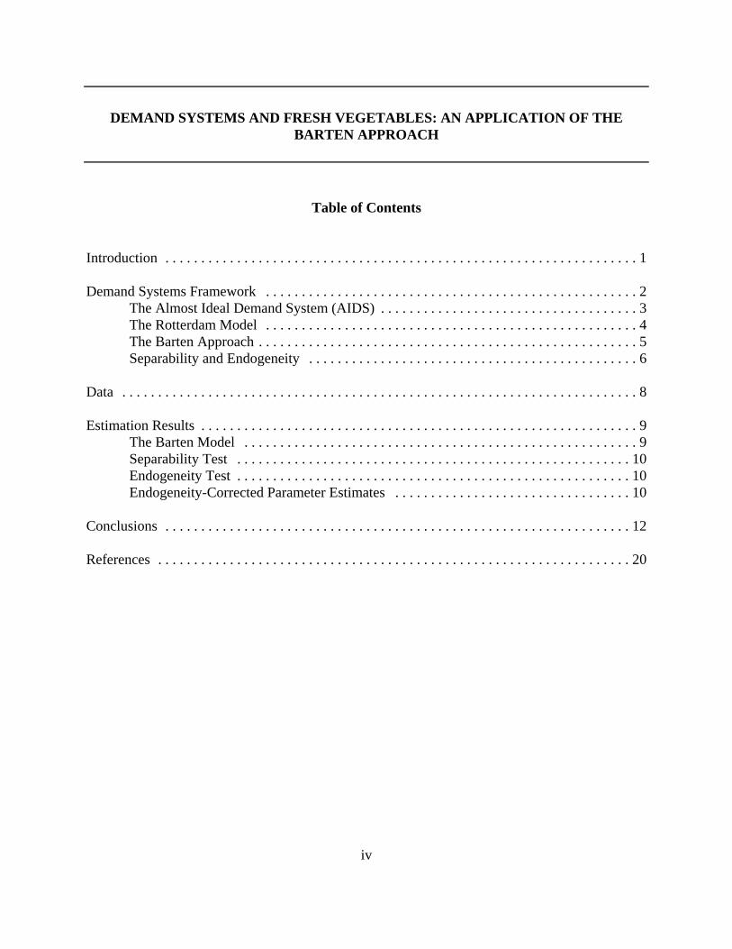
Table of Contents

Introduction . . . . . . . . . . . . . . . . . . . . . . . . . . . . . . . . . . . . . . . . . . . . . . . . . . . . . . . . . . . . . . . . . . 1

Demand Systems Framework . . . . . . . . . . . . . . . . . . . . . . . . . . . . . . . . . . . . . . . . . . . . . . . . . . . . 2The Almost Ideal Demand System (AIDS) . . . . . . . . . . . . . . . . . . . . . . . . . . . . . . . . . . . . 3The Rotterdam Model . . . . . . . . . . . . . . . . . . . . . . . . . . . . . . . . . . . . . . . . . . . . . . . . . . . . 4The Barten Approach . . . . . . . . . . . . . . . . . . . . . . . . . . . . . . . . . . . . . . . . . . . . . . . . . . . . . 5Separability and Endogeneity . . . . . . . . . . . . . . . . . . . . . . . . . . . . . . . . . . . . . . . . . . . . . . 6

Data . . . . . . . . . . . . . . . . . . . . . . . . . . . . . . . . . . . . . . . . . . . . . . . . . . . . . . . . . . . . . . . . . . . . . . . . 8

Estimation Results . . . . . . . . . . . . . . . . . . . . . . . . . . . . . . . . . . . . . . . . . . . . . . . . . . . . . . . . . . . . . 9The Barten Model . . . . . . . . . . . . . . . . . . . . . . . . . . . . . . . . . . . . . . . . . . . . . . . . . . . . . . . 9Separability Test . . . . . . . . . . . . . . . . . . . . . . . . . . . . . . . . . . . . . . . . . . . . . . . . . . . . . . . 10Endogeneity Test . . . . . . . . . . . . . . . . . . . . . . . . . . . . . . . . . . . . . . . . . . . . . . . . . . . . . . . 10Endogeneity-Corrected Parameter Estimates . . . . . . . . . . . . . . . . . . . . . . . . . . . . . . . . . 10

Conclusions . . . . . . . . . . . . . . . . . . . . . . . . . . . . . . . . . . . . . . . . . . . . . . . . . . . . . . . . . . . . . . . . . 12

References . . . . . . . . . . . . . . . . . . . . . . . . . . . . . . . . . . . . . . . . . . . . . . . . . . . . . . . . . . . . . . . . . . 20

v

List of Tables

Table 1. Barten Model Test Results (Including Onions). . . . . . . . . . . . . . . . . . . . . . . . . . . . . . . 14Table 2. U.S. Rotterdam Model Onion Separability Test Results. . . . . . . . . . . . . . . . . . . . . . . . 14Table 3. Barten Model Test Results (Onions Excluded). . . . . . . . . . . . . . . . . . . . . . . . . . . . . . . 15Table 4. U.S. Rotterdam Model - Endogeneity of Expenditures Test Results. . . . . . . . . . . . . . 15Table 5. U.S. Winter Fresh Vegetable Rotterdam Model Parameter Estimates (3SLS)

(Corrected for Endogeneity). . . . . . . . . . . . . . . . . . . . . . . . . . . . . . . . . . . . . . . . . . . . . 16Table 6. U.S. Summer Fresh Vegetable Rotterdam Model Parameter Estimates (3SLS)

(Corrected for Endogeneity). . . . . . . . . . . . . . . . . . . . . . . . . . . . . . . . . . . . . . . . . . . . . 17Table 7. U.S. Winter Fresh Vegetable Elasticities, Rotterdam Model.* . . . . . . . . . . . . . . . . . . 18Table 8. U.S. Summer Fresh Vegetable Elasticities, Rotterdam Model.* . . . . . . . . . . . . . . . . . 19

DEMAND SYSTEMS AND FRESH VEGETABLES: AN APPLICATION OF THEBARTEN APPROACH

U.S. per capita consumption of fresh vegetables increased steadily, even dramatically, during the1980s and 1990s. The main factors behind these trends are related to U.S. population demographicchanges, high income demand elasticities, and changes in consumer preferences. Increased healthconsciousness of U.S. consumers combined with growing information about the potential cancer-preventing qualities of vegetables have contributed to the surge in fresh vegetable demand(McCracken 1992, Málaga and Williams 1996). Growing produce imports from Mexico and rapidgains in production efficiencies have kept fresh vegetable prices declining in real terms, fosteringgrowth in consumption. Accuracy in the measurement of fresh vegetable demand parameters in boththe U.S. and Mexico is key to evaluating the future profitability of the U.S. fresh vegetable industryin the context of a North American free trade area.

Although fresh vegetables are mainly consumed in salads, traditional demand estimation,emphasizing tomatoes and onions, has adopted a single demand equation approach, neglectingimportant interrelationships among demand schedules. However, in recent years, demand systemtechniques have been developed to simultaneously estimate the parameters of closely relateddemands, incorporating the constraints of modern demand theory (adding up, homogeneity, andsymmetry). Unfortunately, the use of alternative demand system formulations (Rotterdam, AIDS,and others) can provide different elasticity estimates.

Only two serious attempts (Mittelhammer 1978 and Scott 1991) have been made to use demandsystems to estimate the parameters for U.S. fresh vegetable demand. In both cases, the selection ofthe demand system was arbitrary with Mittelhammer choosing a mixed statistical estimation methodand Scott using an inverse Rotterdam model.

Mittelhammer estimated U.S. demand schedules at retail and at the farm level for seven “salad”vegetables as a subsystem. The fresh vegetables included tomatoes, cucumbers, bell peppers,lettuce, carrots, celery, and cabbage. The selection of these vegetables was based on a nationalconsumer survey regarding the most used vegetables in salads. The mixed statistical estimationmethod utilized to derive the demand parameters incorporated linear probabilistic constraints,including symmetry, homogeneity and negativity. As hypothesized, he found significantcomplementary and substitution relationships.

The inverse Rotterdam demand model utilized by Scott included four regional demand systems fortomatoes, cucumbers, bell peppers, and green beans. Monthly data over a ten year period was usedfor the terminal markets of New York, Los Angeles, Chicago, and Atlanta. He found significantown and cross-price elasticities with strong complementary relationships in all four markets.

2

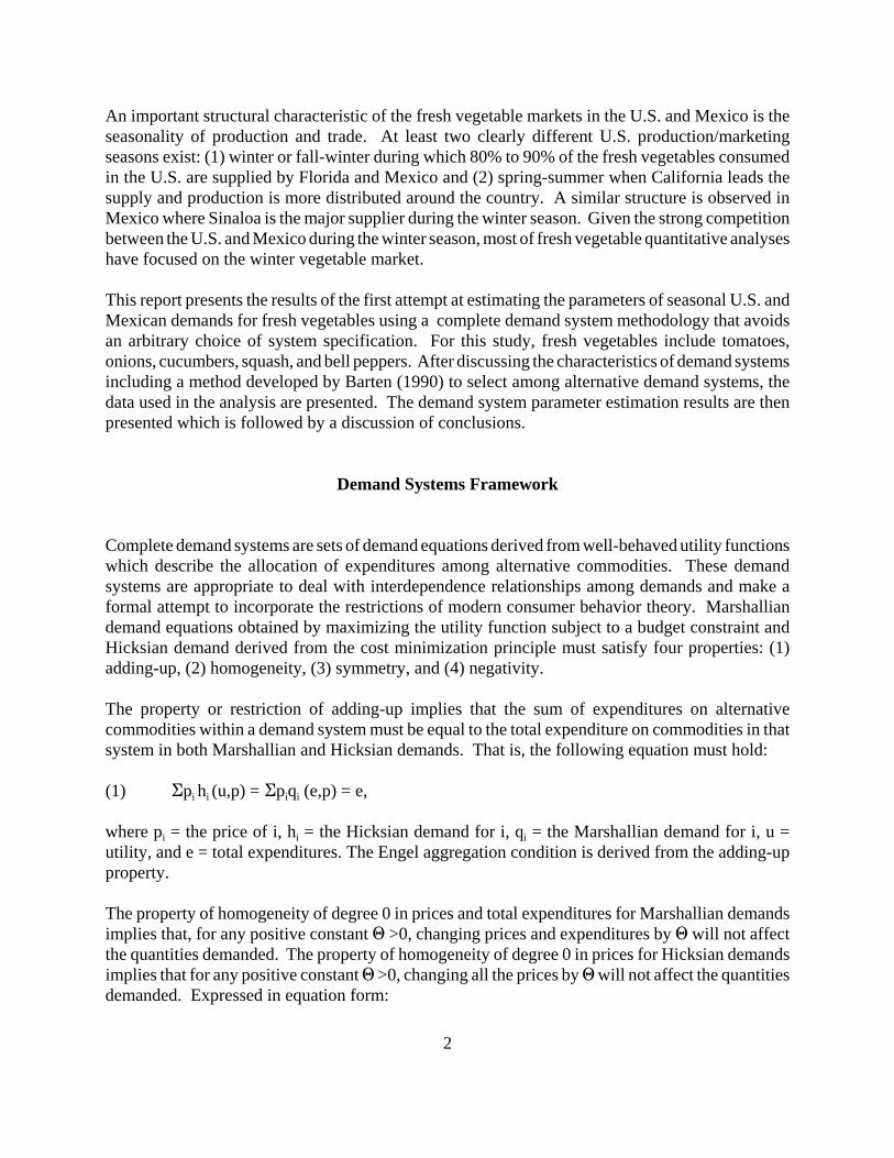
An important structural characteristic of the fresh vegetable markets in the U.S. and Mexico is theseasonality of production and trade. At least two clearly different U.S. production/marketingseasons exist: (1) winter or fall-winter during which 80% to 90% of the fresh vegetables consumedin the U.S. are supplied by Florida and Mexico and (2) spring-summer when California leads thesupply and production is more distributed around the country. A similar structure is observed inMexico where Sinaloa is the major supplier during the winter season. Given the strong competitionbetween the U.S. and Mexico during the winter season, most of fresh vegetable quantitative analyseshave focused on the winter vegetable market.

This report presents the results of the first attempt at estimating the parameters of seasonal U.S. andMexican demands for fresh vegetables using a complete demand system methodology that avoidsan arbitrary choice of system specification. For this study, fresh vegetables include tomatoes,onions, cucumbers, squash, and bell peppers. After discussing the characteristics of demand systemsincluding a method developed by Barten (1990) to select among alternative demand systems, thedata used in the analysis are presented. The demand system parameter estimation results are thenpresented which is followed by a discussion of conclusions.

Demand Systems Framework

Complete demand systems are sets of demand equations derived from well-behaved utility functionswhich describe the allocation of expenditures among alternative commodities. These demandsystems are appropriate to deal with interdependence relationships among demands and make aformal attempt to incorporate the restrictions of modern consumer behavior theory. Marshalliandemand equations obtained by maximizing the utility function subject to a budget constraint andHicksian demand derived from the cost minimization principle must satisfy four properties: (1)adding-up, (2) homogeneity, (3) symmetry, and (4) negativity.

The property or restriction of adding-up implies that the sum of expenditures on alternativecommodities within a demand system must be equal to the total expenditure on commodities in thatsystem in both Marshallian and Hicksian demands. That is, the following equation must hold:

(1) Gpi hi (u,p) = Gpiqi (e,p) = e,

where pi = the price of i, hi = the Hicksian demand for i, qi = the Marshallian demand for i, u =utility, and e = total expenditures. The Engel aggregation condition is derived from the adding-upproperty.

The property of homogeneity of degree 0 in prices and total expenditures for Marshallian demandsimplies that, for any positive constant 1 >0, changing prices and expenditures by 1 will not affectthe quantities demanded. The property of homogeneity of degree 0 in prices for Hicksian demandsimplies that for any positive constant 1 >0, changing all the prices by 1 will not affect the quantitiesdemanded. Expressed in equation form:

3

(2) hi (u, 1p) = hi (h,p) = qi (1x,1p) = qi (e,p) The symmetry property of the cross-price derivatives of the Hicksian demand is implied by Young’stheorem. Thus, in a Hicksian constant utility demand system, the effect of the price of commodityj on the demand for commodity i is equal to the effect of the price of commodity i on the demandfor commodity j, or:

(3) Mhi (u,p)/Mpj = Mhj (u,p)/Mpi, œ i …j .

The negativity condition of Hicksian demands implies that the own-price derivatives will benegative because the Slutzky matrix of elements Mhi/Mpj = sij is negative semi-definite, a conditionderived from the concavity of well-behaved cost functions.

A demand system approach usually incorporates these restrictions into one model to ensure thatconsumer behavior in the model is consistent with theory. Additionally, imposing the classicalrestrictions allows economies of parameterization, always important when dealing with time seriesdata. Moreover, these restrictions when appropriately imposed, are useful in an econometric sense,permitting gains in efficiency of estimation and likely reducing multicollinearity. These advantagesare encouraging agricultural economists to use complete demand systems instead of the moreconventional “ad-hoc” single demand equation approach for investigating the statisticalcharacteristics of consumer behavior. Unfortunately, even when the demand system approach is selected, theory does not provide muchinformation about the “true “ form of the demand functions. Several approaches have developedspecifications that approximate the true form and allow some of the theoretical properties of demandto be imposed or tested. The most used approaches in agricultural economics are: (1) the “AlmostIdeal Demand System” or “AIDS” and (2) the Rotterdam model.

The Almost Ideal Demand System (AIDS)

The AIDS model was developed by Deaton and Muelbauer (1980) as an arbitrary first orderapproximation to any demand system. It satisfies the axioms of choice exactly and aggregatesperfectly over consumers up to a market demand function. Its flexible functional form is consistentwith known household-budget data and can be used to test the properties of homogeneity andsymmetry through linear restrictions on fixed parameters. The AIDS linear approximation suggestedby Stone is usually used (LA/AIDS) and can be specified as:

(4) wit = "i + Ej (i j lnpjt + $ i ln[Yt /Pt* ] + ,it

where wit = expenditure share of product i, pjt = nominal price of product j, Yt = expenditure on theset of products, ,it = disturbance term, ", $, and ( = parameters to estimate, Pt

* = wkt lnpkt = Stone’slinear approximation

4

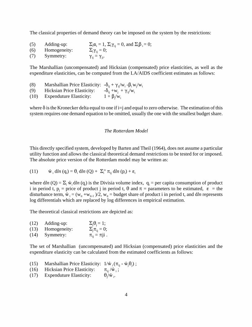
The classical properties of demand theory can be imposed on the system by the restrictions:

(5) Adding-up: Ei"i = 1, Ei(ij = 0, and Ei$ i = 0;(6) Homogeneity: Ei(ij = 0;(7) Symmetry: (ij = (ji.

The Marshallian (uncompensated) and Hicksian (compensated) price elasticities, as well as theexpenditure elasticities, can be computed from the LA/AIDS coefficient estimates as follows:

(8) Marshallian Price Elasticity: -*ij + (ij/wi -$i wj/wi(9) Hicksian Price Elasticity: -*ij +wj + (ij/wi (10) Expenduture Elasticity: 1 + $j/wi

where * is the Kronecker delta equal to one if i=j and equal to zero otherwise. The estimation of thissystem requires one demand equation to be omitted, usually the one with the smallest budget share.

The Rotterdam Model

This directly specified system, developed by Barten and Theil (1964), does not assume a particularutility function and allows the classical theoretical demand restrictions to be tested for or imposed.The absolute price version of the Rotterdam model may be written as:

(11) ë i dln (qi) = 2i dln (Q) + Ein Bij dln (pi) + gi

where dln (Q) = Ei ëi dln (qi) is the Divisia volume index, qi = per capita consumption of producti in period t, pj = price of product j in period t, 2 and B = parameters to be estimated, g = thedisturbance term, ë i = (wit +wit-1 )/2, wit = budget share of product i in period t, and dln representslog differentials which are replaced by log differences in empirical estimation.

The theoretical classical restrictions are depicted as:

(12) Adding-up: Ej2j = 1;(13) Homogeneity: EjBij = 0;(14) Symmetry: Bij = Bji .

The set of Marshallian (uncompensated) and Hicksian (compensated) price elasticities and theexpenditure elasticity can be calculated from the estimated coefficients as follows:

(15) Marshallian Price Elasticity: 1/ë i (Bij - ëj2j) ;(16) Hicksian Price Elasticity: Bij /ë i ;(17) Expenduture Elasticity: 2j/ë i.

5

When estimating any of both demand system models, one equation must be omitted to avoid thesingularity of the variance-covariance matrix of disturbances. The parameters associated with theomitted demand equation can be recovered by making use of the classical restrictions.

The Barten Approach

Since the appearance of the complete demand systems concept, its use by agricultural economistshas grown. Huang estimated a complete food demand system for the U.S. using aggregatecategories (1985). Wahl (1989) and Tsai (1994) used AIDS models to analyze the meat demand inJapan and Taiwan, respectively. Capps et al.(1994) used a Rotterdam system to estimate meatdemand parameters in the Pacific Rim countries. Mittelhammer (1978) used a system approach toestimate the parameters of the U.S. “salad” vegetable demand. Scott (1991) used an inverseRotterdam model to analyze fresh vegetable demands in four selected U.S. terminals.

Only a few studies have used complete demand systems to estimate the parameters of Mexican fooddemands. Heien (1989) used a LA/AIDS model to analyze protein-supplying food demand inMexico. Minert (1994) used also a AIDS model to study meat demand in Mexico. García Vega(1995) compared the LA/AIDS and Rotterdam model estimates of Mexican meat demandparameters. No demand system study has been performed for Mexican vegetable demand.

García Vega (1995) demonstrated that the coefficient and elasticities derived from different demandsystems may differ substantially, posing a relevant question about the appropriate choice of demandsystem specification. Comparisons between alternative specifications can be and have been doneby using goodness-of-fit criteria. Such comparisons have been termed “naive” in that the statisticalinterpretation is not clear (Barten 1990). Because the dependant variables are not the same for thevarious systems, the R2 as a measure of goodness-of-fit is not a particularly useful measure ofrelative performance of demand systems. Moreover, a comparison between full demand systemsrather than between individual equations is most appropriate. Statistical test procedures must takeinto account that the models being compared are not nested within each other.

An alternative approach developed by Barten (1990) allows for a more appropriate method ofdemand system selection. The Barten technique artificially nests four versions of differentialdemand systems (Rotterdam, AIDS, NBR, and CBS) in a more general model using the VariableAddition Method of McAleer (1983). The method was extended to a combination of vector valuefunctions and applied to a comparison of the demand systems. Given the nature of the dependentvariables, the test basically reduces to assessing the extra explanatory power of the vectors ofexogenous variables. The Likelihood Ratio Test statistic can be used for this purpose (Barten 1990).The general Barten model specification can be written as:

(18) ë i dln (qi) = di dln (Q) + Ej eij dln (pj ) +*1 [ë i dln (Q)] - *2 {ë i [dln (pi ) - dln (P)]}

where: ë i = (wit +wit-1 )/2; dln (qi) = ln (qit +qit-1 ); dln (pi) = ln (pit +pit-1 ); dln (Q) = Ei ë i dln (qi),;

6

dln (P) = Ei ë i dln (pi); wit = budget share of product i in period t; *1 = coefficient associated withthe difference between the Rotterdam and the CBS system (Rotterdam and AIDS expenditurecoefficients); *1 = coefficient associated with the difference between the Rotterdam and the NBRsystems (Rotterdam and AIDS price coefficients).

When the coefficients *1 and *2 are equal to zero, the Barten general model is equivalent to theRotterdam model. When *1 and *2 are equal to one, the Barten model is transformed into an AIDSmodel. Other combinations are also possible representing the NBR and CBS models. Therefore,determining which is the most appropriate demand system model for a particular set of data reducesto an empirical test of the values of *1 and *2. The Likelihood Ratio Test can be used for thispurpose. In this study case, the Barten approach is used to determine whether Rotterdam or AIDSis the suitable model for the fresh vegetable demand system in the U.S. and Mexico.

Separability and Endogeneity

Demand system studies for U.S. fresh vegetables have not included onions as part of the system.Mittelhammer (1978) did not include onions in his U.S. salad vegetable system because of a lackof adequate data. However, he refers to a U.S. Department of Agriculture (USDA) nationwidesurvey which concludes that consumers consider white onions to be a “salad” vegetable. Otherstudies simply assumed that onions “did not belong” to the fresh vegetable system.

Fortunately, the available demand systems methodologies allow for a separability tests. These testscan be used to determine whether a particular commodity, in this case onions, should be includedin a demand system. A test based on the assumption of weak separability of the direct utilityfunction will be used. With that assumption, Goldman and Uzawa (1964) showed that:

(19) Sij =Nij (Mqi /Me)(Mqj / Me), i 0 I, j0 J

where I refers in these case to the group of fresh vegetables other than onions; J alludes to the singlecommodity, in this case onions; Sij represents the Slutzky substitution term; Nij is a substitutabilityparameter between commodities in groups I and J; and Mqi /Me and Mqj / Me are the derivatives ofproducts i and j with respect to total expenditure.

With some algebraic manipulation it can be shown that:

(20) ,*ij = (Nij /e) ni nj wj ,

where, ,*ij refers to the compensated cross price elasticity between commodities in groups I and J;

ni and nj are the expenditure elasticities of products in the two respective groups; and wj is thebudget share of commodity j. Also for i, k 0 I and j 0 J, equation (20) can be used to demonstratethat:

7

(21) ,*ij/,*

kj = ni /nk.

In other words, under the assumption of weak separability of the direct utility function, the ratio ofHicksian or compensated cross-price elasticities of two commodities in the same group with respectto a third commodity in another group is equal to the ratio of their respective expenditure elasticities.In the context of the Rotterdam model, (21) implies a nonlinear restriction on the parameters Bij ,where the i and k 0 I, and j0 J. This Rotterdam parameter restriction can be written as:

(22) Bij /Bkj = 2i /2k.

In this study, i and k 0 I include tomatoes, cucumbers, bell peppers, and squash, and j0 J refers toonions. The separability test becomes a Likelihood Ratio Test of the hypothesis of the separabilityof onions. In the case of the AIDS model, a similar test can be performed.

Another relevant issue when dealing with food demand systems is the assumption of endogeneityof total expenditures. Since by definition total expenditures are the sum of expenditures on eachcommodity, total expenditures are generally expected to be endogenously determined. However,if the total expenditures variable is correlated with the equation error, the parameter estimates couldbe biased and inconsistent.

To deal with this problem, Capps et al. (1994) applied a technique developed by Attfield (1985) andby Hausman (1977). For the case of the Rotterdam model, this procedure requires the estimationof an n-equation system of the following form:

(23) ë i dln (qi) = 2i [ "0 + Ekm "k Zk ] + Ej

n Bij dln (pj )+ gi, i =1,...n-1dln (Q) = "0 + Ek

m "k Zk + :,

where 2i ,Bij, "0, and "k are structural parameters; and Zk corresponds to a set of predeterminedvariables including dln (pj ).

Therefore, this procedure includes an additional equation in the demand system which is a regressionof the total expenditure variable dln (Q) on a set of exogenous variables (which, in this study,include the log differences of the prices of tomatoes, onions, cucumbers, bell peppers, and squash,and the log difference of real per capita income). The hypothesis that the parameters "k are jointlyequal to zero can then be tested. If the hypothesis is rejected, the estimates of both the price andexpenditure coefficients in the demand system would have been biased and inconsistent. In otherwords, total expenditures are not endogenous and its correlation with the disturbance term needs tobe taken into account. This is done by keeping the extra equation as part of the demand system forestimation.

Data

8

As discussed previously, important production, marketing, and trade patterns clearly differentiatethe two main fresh vegetable seasons in the U.S. and in Mexico. Except for onions, where somedegree of storage exists in the U.S., the perishable nature of these vegetables does not allow forinventory carry over from one season to another. Preliminary research determined that eachproductive season in each constitutes an independent system with no relevant linkages betweenthem. Consequently, in attempting to model the fresh vegetable markets in each country, eachseason must be accounted for separately. According to U.S. and Mexican production data, thewinter season covers vegetable production and consumption corresponding to the months ofDecember through May in both countries while the summer season covers the months of Junethrough November. Monthly data were converted into seasonal data using these seasonaldefinitions. Because of data limitations, only five fresh vegetables were included in the analysis:(1) tomatoes, (2) onions, (3) cucumbers, (4) squash, and (5) bell peppers. These vegetables are themost traded between both countries and, except for lettuce, account for most of fresh vegetableconsumption. The available data allowed for a period of analysis of 1971 through 1993.

U.S. monthly shipment data from the USDA Agricultural Marketing Service (AMS) were used tocalculate seasonal weights for the production of each vegetable. The annual production figures ofthe USDA National Agricultural Statistics Service (NASS) and the seasonal shipment structure wereused to determine the U.S. seasonal production following the method used by the EconomicResearch Service (ERS) to estimate monthly production levels. U.S. imports from Mexico wereprovided by AMS. Imports from other countries, U.S. exports, and border prices were obtained fromthe U.S. Bureau of the Census (USBC) and the U.S. Department of Commerce (USDC). Retailprices were obtained from the Bureau of Labor Statistics, U.S. Department of Labor. During 1982 through 1991 when USDA discontinued publication of national level data forcucumbers and bell peppers, national production was calculated as production-weighted averagesof the corresponding data obtained from the Agricultural Statistical Services of the major producingstates (Florida, California, Texas, Georgia, New Jersey, New York, Virginia Arizona, Michigan, andNorth Carolina). Because squash production statistics were available only for Florida, those datawere used to represent national data. Seasonal per capita apparent consumption was computed fromthe production, trade, and population figures.

Mexican seasonal production data were obtained primarily from Anuario Estadístico de laProducción Agrícola de los Estados Unidos Mexicanos published by the Secretaría de Agricultura,Ganadería y Desarrollo Rural (SAGAR). For the years 1986-1988 when SAGAR data werediscontinued, state level data from major producing states were collected from DelegacionesEstatales de la SAGAR and unpublished SAGAR data provided by the Center for Economic, Social,and Technology Research on World Agriculture and Agribusiness (CIESTAAM) at the AutonomousUniversity of Chapingo in Mexico (Gómez Cruz, Rindermann, and Merino 1991 and UniversidadAutónoma de Chapingo 1992). Apparent Mexican consumption was calculated using Mexicanseasonal production and trade.

Retail prices in Mexico were calculated using the monthly retail price indices for tomatoes, onions,cucumbers, and squash published by the Banco de Mexico (1993) in the Cuaderno Mensual Indice

9

de Precios. Those indices were transformed into a series of absolute prices using the Banco deMexico actual prices for January 1989 which were then converted into seasonal averages. Becauseconsistent official monthly data for Mexican exports do not exist, U.S. statistics of monthly importsfrom Mexico were assumed to correspond to Mexican exports. Mexican monthly consumer priceindices were taken from the International Financial Statistics (IMF). Retail prices in both countrieswere deflated by the respective CPI index.

Estimation Results

To determine the appropriate demand system model for fresh vegetable demand in each country,the Barten approach described earlier was used. The selected demand system was subjected toendogeneity and separability tests and the parameters re-estimated. Because previous studies haveassumed that onions are not considered to be a “salad” vegetable, a test for separability of onionswas conducted to confirm or reject the hypothesis that onions belong to the “salad” vegetable group.A test for endogeneity of expenditures was also performed. The three stage least squares (3SLS)systems estimator was used to derive the parameters of the system because endogenous variablesin some equations of the model were used as explanatory variables in other equations (systemsimultaneity).

The Barten Model

The Barten model for the five selected vegetables (tomatoes, onions, cucumbers, squash, and bellpeppers) was used for both the winter and the summer season models for the U.S. and Mexico. TheBarten models for Mexico did not include bell peppers. For the U.S. in both the winter and summerseasons, the Barten model likelihood ratio tests indicated rejection of the Almost Ideal DemandSystem (AIDS) model but failed to reject the Rotterdam model (Table 1). In the case of Mexico inboth seasons, both AIDS and Rotterdam systems were rejected except for the summer Rotterdammodel.

Separability Test

A test for weak separability of onion demand, as described above, was performed using theRotterdam model for the United States. Mittelhammer (1978) argues that onions have multiple fooduses and might not be a typical “salad” vegetable except for white onions. The test failed to rejectthe null hypothesis of weak separability of onions at the 0.05 significance level of the i2 distribution(Table 2). This outcome suggests that onion demand can be separated from the other fresh vegetabledemands for analytical purposes. Subsequent demand system analyses will include, therefore, onlytomatoes, cucumbers, squash, and bell peppers. Onion demand will be modeled separately.

10

A new Barten model, without onions, was then estimated to confirm the appropriateness of theRotterdam specification for the fresh vegetable demand system of both countries. The AIDS modelwas again rejected in all cases while the Rotterdam model was not rejected except for the winterseason vegetable demand in Mexico (Table 3).

Endogeneity Test

Another concern in the analysis of demand systems is the endogeneity of total expenditures.Because fresh vegetable consumption likely increases with the level of education and income, totalconsumer expenditures for fresh vegetables might not be exogenous to the demand system as theoriginal Rotterdam model assumes leading to biased and inconsistent parameter estimates (Capps,et al. 1994). To get around this problem, the technique developed by Attfield (1985) and Hausman(1977) can be used which involves extending the demand system with a regression of the totalexpenditure variable (Q) on a set of exogenous variables including the log differences of the pricesof each one of the included fresh vegetables and the log difference of real per capita income.

The structural parameters of the augmented demand system are then estimated using the nonlinearmaximum likelihood algorithm in the SHAZAM econometrics package. The hypothesis that theparameters of the augmented equation are jointly equal to zero can be tested. This hypothesis wasrejected for the U.S. fresh vegetable model in both seasons using the likelihood ratio test at 0.05significance (Table 4). This result implies that exogeneity of total expenditures cannot be assumedand that the parameters of the Rotterdam model would be biased and inconsistent if the correlationof total expenditure and the disturbance terms was not taken into account.

Endogeneity-Corrected Parameter Estimates

Based on the results of the endogeneity test, the augmented equation was kept in the Rotterdammodel of the U.S. fresh vegetable demand system. The Rotterdam model for Mexican vegetabledemand yielded parameters of low statistical significance with some elasticity levels outsidereasonable ranges and the results are not provided in this paper.

The parameters of all but one of the demand equations in the endogeneity-corrected Rotterdammodel for the United States in the winter and summer seasons were estimated directly because theadding-up constraint implies that only three of the four demand equations are independent (Tables5 and 6). The bell pepper demand equation was omitted from estimation but its parameters wererecovered using the classical restrictions from demand theory.

The R2 statistics are somewhat low across the board with the highest for the tomato demandequations in the winter and summer seasons (0.88 and 0.83, respectively). Serial correlation, asmeasured by the Durbin-Watson (DW) coefficient, was not evident in any of the equations in either

11

season, except perhaps for the summer tomato demand equation. The t-values corresponding to theestimated coefficients indicate that only four winter parameter estimates and three summer estimatesare significant at 0.05 significance level (Tables 5 and 6).

The Hicksian (income-compensated) and Marshallian (income-uncompensated) elasticities derivedfrom the Rotterdam model were derived at the sample means of the data (Tables 7 and 8 for thewinter and summer seasons, respectively). Winter Marshallian elasticities are generally within theexpected range according to previous studies (Table 7). All own-price winter Marshallianelasticities are negative and all but one are significant at 0.05 level. Own-price elasticities rangefrom -0.21 for bell peppers to -0.53 for tomatoes. Except for the bell pepper-cucumber case, allwinter cross-price Marshallian elasticities are negative, implying gross complementarity of therespective commodities in consumption. Only half the winter Hicksian cross-price elasticities arenegative implying that some gross complements are net substitutes. Winter expenditure elasticitiesare relatively high, ranging from 0.85 for tomatoes to 1.35 for cucumbers.

Summer Marshallian own-price elasticities are also negative in all cases (Table 8), from -0.17 forcucumbers to -0.63 for tomatoes. As is the case for the winter demand equations, most cross-priceelasticities are negative. Only four summer demand elasticities indicate substitution in consumption(squash-cucumbers and bell pepper-squash). Only three summer Marshallian cross-price elasticitiesare significant at 0.05 level. Summer expenditure elasticities range from 0.74 for tomatoes to 1.7for bell peppers.

The Marshallian own-price elasticities for winter and summer tomato and squash demand are similarin magnitude. The cucumber own-price elasticity is higher in the summer season and that of bellpeppers is higher in the winter season. The magnitudes and signs of Marshallian cross-pricerelationships also change with the season. For example, squash and cucumbers are grosscomplements in winter but gross substitutes in summer. Similarly, squash is a gross substitute ofbell peppers in winter but a gross complement in summer. In general, though, complementaryrelationships are more common in the winter season which may be related to seasonal differencesin consumption habits and produce availabilities. Expenditure elasticities are in the same range inboth seasons, except for bell peppers (clearly higher in summer). In both seasons, all cross-priceelasticities with respect to tomatoes are positive and high in magnitude, suggesting that tomatoesare the primary salad vegetable.

The magnitudes of the Marshallian own-price elasticities are in general agreement with the resultsof previous studies. Tomato own-price elasticities for winter demand (-0.53) and summer demand(-0.63) are very close to the annual elasticity reported by Huang in 1985 (-0.56), Simmons in 1987(-0.50), and somewhat above the magnitudes found by Salcedo Baca in 1990 (-0.31), Mittelhammerin 1978 (-0.42), and Gutiérrez (1983) for the winter season in 1988 (-0.44). Shonkwiler andEmerson (1980) report a winter tomato own-price elasticity of -0.79.

The winter cucumber uncompensated own-price elasticity of -0.51 corresponds closely to theelasticity reported by Mittelhammer in 1978 (-0.54) and that reported by Castro and Simmons in1974 (-0.57). Similarly, the winter bell pepper elasticity of -0.21 is close to that found by

12

Mittelhammer (-0.23). However, the estimated own-price elasticities for summer cucumber and bellpepper demand are quite different from their respective annual elasticities reported in previousstudies. Unfortunately, there have been no previous studies of squash demand to allow a comparisonwith the winter squash own-price elasticity of -0.32 found in this study.

The tomato expenditure elasticities of 0.85 for winter demand and 0.74 for summer demand foundin this study are above those estimated for the entire year by Huang (0.49) and Mittelhammer (0.29)and below the income elasticities for tomatoes reported by Shonkwiler and Emerson in 1982 (2.09),Gutierrez in 1988 (1.47), and Salcedo Baca in 1990 (2.60). Expenditure elasticities reported herefor winter and summer cucumbers (1.3 and 1.5, respectively) and for winter and summer bellpeppers (1.1 and 1.7, respectively) are much higher than the expenditure elasticities reported byMittelhammer in 1978 (0.23 for cucumbers and 0.43 for bell peppers). No previous study reportsexpenditure or income elasticities for squash.

The differences found between the seasonal own and cross-price elasticities for some vegetablessupports the general hypothesis that there are important structural differences in the nature of theseasonal demands for vegetables, probably related to salad consumption habits. Moreover, thedifferent signs of some cross-price elasticities between seasons reinforce the appropriateness of theseasonal separation of fresh vegetable demand for analytical purposes.

Conclusions

The results of this study indicate that the Rotterdam model is the most appropriate demand systemfor the estimation of fresh vegetables demand parameters for both the winter and summer seasonsin both the U.S. and Mexico. Hicksian, Marshallian and expenditure elasticities are calculatedseparately for each season. Own- and cross-price elasticities display seasonal differences. A weakseparability test suggests that onions are separable or that they do not belong to the “salad vegetable”demand system. Finally, likelihood test results imply that exogeneity of total expenditures cannotbe assumed and that the parameters of the Rotterdam model would be biased and inconsistent if thecorrelation of total expenditures and the disturbance terms is not taken into account.

Consequently, the Rotterdam model appears to be the appropriate demand system for estimating theparameters of the demand for fresh vegetables in both the U.S. and Mexico. Onion demandequations apparently do not belong to the fresh vegetable demand group. Marhsallian andexpenditure elasticities are found to be within expected ranges. While tomato and squash own-priceelasticities are about the same in fall-winter and spring-summer seasons, cucumber and bell pepperown-price elasticities display substantial seasonal differences. Except for tomatoes, expenditureelasticities are all above one suggesting that most fresh vegetables could be considered luxurygoods.

14

Table 1. Barten Model Test Results (Including Onions).

Season/ModelLog Likelihood

(Restricted)Log Likelihood(Unrestricted)

LikelihoodRatio

Hypothesis TestP2 at 0.05 level 1

U.S. Winter

AIDS 315.95 325.33 18.75 Reject Ho

Rotterdam 323.30 325.33 4.06 Fail to Reject Ho

U.S. Summer

AIDS 316.66 320.79 8.25 Reject Ho


Mexico Winter

AIDS 138.95 143.41 8.92 Reject Ho

Rotterdam 138.14 143.41 10.54 Reject Ho

Mexico Summer

AIDS 172.86 177.71 9.70 Reject Ho

Rotterdam 176.21 177.71 3.00 Fail to Reject Ho1 Critical value for P2 at 0.05 level and two degrees of freedom: 5.99

Table 2. U.S. Rotterdam Model Onion Separability Test Results.

SeasonLog Likelihood


LikelihoodRatio


Winter 314.82 319.42 8.39 Fail to Reject Ho

Summer 312.45 314.86 4.86 Fail to Reject Ho1 Critical value for P2 at 0.05 level and four degrees of freedom: 9.49

15

Table 3. Barten Model Test Results (Onions Excluded).

Season/ModelLog Likelihood


LikelihoodRatio


U.S. Winter

AIDS 218.45 230.34 22.99 Reject Ho


U.S. Summer

AIDS 234.21 237.73 7.05 Reject Ho


Mexico Winter

AIDS 92.80 102.70 19.82 Reject Ho

Rotterdam 89.92 102.70 25.56 Reject Ho

Mexico Summer

AIDS 122.51 126.63 8.22 Reject Ho

Rotterdam 125.09 126.63 3.08 Fail to Reject Ho1 Critical value for P2 at 0.05 level and two degrees of freedom: 5.99

Table 4. U.S. Rotterdam Model - Endogeneity of Expenditures Test Results.

SeasonLog Likelihood


LikelihoodRatio


Winter 219.79 264.4 89.22 Reject Ho

Summer 230.90 268.16 74.51 Reject Ho1 Critical value for P2 at 0.05 level and five degrees of freedom: 11.07

16

Table 5. U.S. Winter Fresh Vegetable Rotterdam Model Parameter Estimates (3SLS)(Corrected for Endogeneity).

Variable Tomatoes Cucumbers Squash B. Peppers Q

Price of Tomatoes -0.0098(-0.29)

0.0089(0.59)

0.0210(1.73)

-0.0201(-0.74)

-0.0731(-0.75)

Price of Cucumbers 0.0089(0.59)

-0.0446(-2.01)

0.0044 (0.59)

0.0313(2.20)

-0.0149(-0.21)

Price of Squash 0.0210(1.73)

0.0044(0.59)

-0.0156(-0.87)

-0.0097(-0.89)

-0.1881(-3.08)

Price of Bell Peppers -0.0201(-0.74)

0.0313(2.20)

-0.0097 (-0.89)

-0.0015(-0.05)

-0.1385(-1.73)

Q 0.5132(8.06)

0.1836(5.12)

0.1030(3.40)

0.2002(2.53)

-

DLINC - - - - 1.1711(3.37)

R-Square 0.88 0.57 0.40 * 0.56

D-W Statistic 1.91 2.01 1.70 * 1.36

* Bell Pepper equation was omitted as discussed in the text. Parameters for this equation were recovered using the classical restrictions of Demand Theory.** t-values are in parentheses.

17

Table 6. U.S. Summer Fresh Vegetable Rotterdam Model Parameter Estimates (3SLS) (Corrected for Endogeneity).

Variable Tomatoes Cucumbers Squash B. Peppers Q

Price of Tomatoes -0.0795(-1.81)

0.0109(0.50)

-0.0045(-0.63)

0.0731(1.99)

-0.0781(-0.72)

Price of Cucumbers 0.0109(0.50)

-0.0015(-0.05)

0.0043(0.71)

-0.0136(-0.85)

0.3190(2.28)

Price of Squash -0.0045(-0.63)

0.0043(0.71)

-0.0049(-0.46)

0.0051(0.91)

-0.0043(-0.11)

Price of Bell Peppers 0.0731(1.99)

-0.0136(-0.85)

0.0051(0.91)

-0.0646(-1.60)

0.0115(0.13)

Q 0.5178(3.90)

0.1502(2.64)

0.0178(0.95)

0.3142(2.16)

-

DLINC - - - - -0.4553(-1.43)

R-Square 0.83 0.25 0.3 * 0.16

D-W Statistic 1.47 2.36 3.19 * 1.71

* Bell Pepper equation was omitted as discussed in the text. Parameters for this equation were recovered using the classical restrictions of Demand Theory.** t-values are in parentheses.

18

Table 7. U.S. Winter Fresh Vegetable Elasticities, Rotterdam Model.*

Marshallian Elasticities

Tomatoes Cucumbers Squash Bell Peppers

Tomatoes -0.529(-5.61)

-0.101(-3.27)

-0.032(-1.36)

-0.189(-4.38)

Cucumbers -0.747(-3.58)

-0.512(-4.64)

-0.073(-1.19)

-0.017(-0.12)

Squash -0.523(-1.71)

-0.122(1.03)

-0.304(-2.78)

-0.364(-2.66)

Bell Peppers -0.768(-2.81)

0.022(0.27)

-0.138(-2.05)

-0.209(-1.42)

Hicksian Elasticities


Tomatoes -0.017(-0.29)

0.015(0.59)

0.035(1.73)

-0.033(-0.75)

Cucumbers 0.065(0.59)

-0.328(-2.01)

0.032(0.59)

0.229(2.20)

Squash 0.268(1.73)

0.056(0.59)

-0.201(-0.87)

-0.123(-0.89)


0.171(2.20)

-0.053(-0.89)

-0.008(-0.05)

Expenditure Elasticities


0.852(8.06)

1.349(5.12)

1.313(3.40)

1.093(2.53)

* t values are in parentheses

19

Table 8. U.S. Summer Fresh Vegetable Elasticities, Rotterdam Model.*

Marshallian Elasticities


Tomatoes -0.632(-4.38)

-0.607(-1.43)

-0.018(-1.64)

-0.032(-0.46)

Cucumbers -0.912(-2.28)

-0.165(-0.70)

0.018(0.31)

-0.402(-2.25)

Squash -1.056(-1.23)

0.153(0.37)

-0.327(-1.60)

0.115(0.31)


-0.183(-2.19)

0.001(0.04)

-0.664(-3.24)

Hicksian Elasticities


Tomatoes -0.114(-1.81)

0.016(0.50)

-0.006(-0.63)

0.105(1.99)

Cucumbers 0.106(0.50)

-0.015(-0.05)

0.004(0.71)

-0.132(-0.85)

Squash -0.279(-0.63)

0.268(0.71)

-0.309(-0.46)

0.320(0.91)

Bell Peppers 0.396(1.99)

-0.074(-0.85)

0.027(0.91)

-0.350(-1.60)

Expenditure Elasticities


0.743(3.90)

1.461(2.64)

1.114(0.95)

1.705(2.16)

*t values are in parentheses

20

References

Attfield, C.L.F. “Homogeneity and Endogeneity in Systems of Demand Equations.” J.Econometrics 27(1985): 197-209.

Banco de Mexico. Indice de Precios. Cuaderno Mensual. Mexico D.F. Various Issues.

Barten, Anton P. “Consumer Allocation Models: Choice of Functional Form.” EmpiricalEconomics 18(1993): 129-158.

Capps, Jr. O., R.Tsai, R.Kirby, and G. Williams. “A Comparison of Demands for Meat Productsin the Pacific Rim Region.” J. of Agr. and Resource Econ. 1(1994): 210-224.

Deaton, A., and J. Muellbauer. Economics and Consumer Behavior. Cambridge, MA:Cambridge University Press, 1980.

García Vega, J., “The Mexican Livestock, Meat, and Feedgrain Industries: A Dynamic Analysisof U.S.-Mexico Economic Integration.” Ph.D. Diss., Texas A&M University, 1995.

Goldman, S.M., and H.Uzawa. “A Note on Separability in Demand Analysis.” Econometrica 32(1964):387-98.

Gómez Cruz, M.A., R.S. Rindermann, and A. Merino. El Consumo de Hortalizas en Mexico.CIESTAAM, Reporte de Investigación 07, Univ. Aut. Chapingo, Mexico, Nov. 1991.

Gutiérrez, N. “Economic Study of the Winter Vegetable Export Industry of Northwest Mexico.”Master Thesis. University of Missouri-Columbia. Dec. 1988.

Hausman, J.A., “Errors in Variables in Simultaneous Equation Models.” J. Econometrics5(1977):389-401.

Heien, D., L.S. Jarvis, and F. Perali. “Food Consumption in Mexico.” Food Policy 14(1989):167-79.

Huang, K. U.S. Demand for Food: A Complete System of Price and Income Effects. TechnicalBulletin # 1795, U.S. Department of Agriculture, Economic Research Service,Washington DC, 1985.

International Monetary Fund (IMF). International Financial Statistics. Washington DC, 1971-94.

Málaga, J. and G.W. Williams. U.S. and Mexican Fresh Vegetable Markets: A DescriptiveAnalysis. International Market Research Report IM 5-96, Texas Agricultural MarketResearch Center, Texas A&M University, Nov. 1996.

21

McAleer, M. “Exact Tests of a Model Against Non-Nested Alternatives.” Biometrika 70(1983):385-288

McCracken, Vicki A. “The U.S. Demand for Vegetables”. Vegetable Markets in the WesternHemisphere. Ames, IA: Iowa State University Press, 1992.

Minert, J., C. Snyder, B. Goodwin, and G. Brester. “Meat Demand in Mexico.” Selected PaperPresented at the 1994 SAEA Meeting, Nashville TN.

Mittelhammer, R.C. “The Estimation of Domestic Demand for Salad Vegetables Using A Priori Information.” Ph.D. Dissertation, Washington State University, 1978.

Salcedo Baca, D. “Distributional Effects of the Mexican Agricultural Trade Policies: TheTomato Case.” Ph.D. Dissertation, University of Illinois at Urbana-Champaign, 1990.

Scott, W.S. “International Competition and Demand in the United States Fresh Winter VegetableIndustry.”M.S. Thesis, University of Florida, 1991.

Secretaria de Agricultura Ganaderia y Desarrollo Rural, SAGAR. Anuario Estadistico de laProduccion Agricola Nacional. Mexico D.F. Various issues.1970-1993.

Tsai, R. “Taiwanese Livestock and Feedgrain Markets: Economic Structure, Policy Intervention,and Trade Liberalization.” Ph.D. Dissertation, Texas A&M University, 1994.

Universidad Autonoma de Chapingo. La Agricultura Mexicana Frente al Tratado Trilateral deLibre Comercio. CIESTAAM, Chapingo, Mexico, 1992.

U.S. Bureau of the Census (USBC). U.S. General Imports for Consumption/Schedule ACommodity by Country. Washington DC, Various issues.

U.S. Department of Agriculture (USDA). Agricultural Marketing Service (AMS). Fresh Fruitand Vegetable Shipments. Washington D.C., 1971-95.

U.S. Department of Agriculture (USDA). Economic Research Service (ERS). Vegetables andSpecialties. Washington D.C., Various issues.

United States Department of Agriculture (USDA). National Agricultural Statistics Service(NASS). Vegetable Summary. Washington DC, Various issues.

United States Department of Commerce (USDC). Bureau of Economic Analysis (BEA).Business Statistics 1961-91, Washington DC, Various issues.

demand systems and fresh vegetables: an ...afcerc.tamu.edu/publications/publication-pdfs/cp 1...

Documents