delay differential equations and applications - mobt3ath.com · 2.2 application to delay...
TRANSCRIPT

Delay Differential Equations and Applications

Series II: Mathematics, Physics and Chemistry – Vol. 205
NATO Science Series
A Series presenting the results of scientific meetings supported under the NATO Science
Programme.
The Series is published by IOS Press, Amsterdam, and Springer in conjunction with the NATO
Public Diplomacy Division
Sub-Series
I. Life and Behavioural Sciences IOS Press
II. Mathematics, Physics and Chemistry Springer
III. Computer and Systems Science IOS Press
IV. Earth and Environmental Sciences Springer
The NATO Science Series continues the series of books published formerly as the NATO ASI Series.
The NATO Science Programme offers support for collaboration in civil science between scientists of
countries of the Euro-Atlantic Partnership Council. The types of scientific meeting generally supported
are “Advanced Study Institutes” and “Advanced Research Workshops”, and the NATO Science Series
collects together the results of these meetings. The meetings are co-organized bij scientists from
NATO countries and scientists from NATO’s Partner countries – countries of the CIS and Central and
Eastern Europe.
Advanced Study Institutes are high-level tutorial courses offering in-depth study of latest advances
in a field.
Advanced Research Workshops are expert meetings aimed at critical assessment of a field, and
identification of directions for future action.
As a consequence of the restructuring of the NATO Science Programme in 1999, the NATO Science
Series was re-organised to the four sub-series noted above. Please consult the following web sites for
information on previous volumes published in the Series.
http://www.nato.int/science
http://www.springer.com
http://www.iospress.nl

Delay Differential Equations and Applications
edited by
O. ArinoUniversity of Pau, France
M.L. HbidUniversity Cadi Ayyad,Marrakech, Morocco
and
E. Ait DadsUniversity Cadi Ayyad,Marrakech, Morocco
Published in cooperation with NATO Public Diplomacy Division

Published by Springer,P.O. Box 17, 3300 AA Dordrecht, The Netherlands.
Printed on acid-free paper
All Rights Reserved
No part of this work may be reproduced, stored in a retrieval system, or transmittedin any form or by any means, electronic, mechanical, photocopying, microfilming,recording or otherwise, without written permission from the Publisher, with the exceptionof any material supplied specifically for the purpose of being enteredand executed on a computer system, for exclusive use by the purchaser of the work.
Proceedings of the NATO Advanced Study Institute on
Marrakech, Morocco9–21 September 2002
A C.I.P. Catalogue record for this book is available from the Library of Congress.
ISBN-10 1-4020-3646-9 (PB)ISBN-13 978-1-4020-3646-0 (PB)ISBN-10 1-4020-3645-0 (HB)ISBN-13 978-1-4020-3645-3 (HB)ISBN-10 1-4020-3647-7 (e-book)ISBN-13 978-1-4020-3647-7 (e-book)
Delay Differential Equations and Applications
www.springer.com
© 2006 Springer

Contents
List of Figures xiii
Preface xvii
Contributing Authors xxi
Introduction xxiiiM. L. Hbid
1History Of Delay Equations 1J.K. Hale
1 Stability of equilibria and Lyapunov functions 32 Invariant Sets, Omega-limits and Lyapunov functionals. 73 Delays may cause instability. 104 Linear autonomous equations and perturbations. 125 Neutral Functional Differential Equations 166 Periodically forced systems and discrete dynamical systems. 207 Dissipation, maximal compact invariant sets and attractors. 218 Stationary points of dissipative flows 24
Part I General Results and Linear Theory of Delay Equations inFinite Dimensional Spaces 29
2Some General Results and Remarks on Delay Differential Equations 31E. Ait Dads
1 Introduction 312 A general initial value problem 33
2.1 Existence 342.2 Uniqueness 352.3 Continuation of solutions 372.4 Dependence on initial values and parameters 382.5 Differentiability of solutions 40
v
vi DELAY DIFFERENTIAL EQUATIONS
Part II Hopf Bifurcation, Centre manifolds and Normal Forms for De-lay Differential Equations 141
4Variation of Constant Formula for Delay Differential Equations 143M.L. Hbid and K. Ezzinbi
1 Introduction 143
2 Variation Of Constant Formula Using Sun-Star Machinery 1452.1 Duality and semigroups 1452.1.1 The variation of constant formula: 1462.2 Application to delay differential equations 1472.2.1 The trivial equation: 1472.2.2 The general equation 149
3 Variation Of Constant Formula Using Integrated SemigroupsTheory 1493.1 Notations and basic results 1503.2 The variation of constant formula 153
3Autonomous Functional Differential Equations 41Franz Kappel
1 Basic Theory 411.1 Preliminaries 411.2 Existence and uniqueness of solutions 441.3 The Laplace-transform of solutions. The fundamental
matrix 461.4 Smooth initial functions 541.5 The variation of constants formula 551.6 The Spectrum 591.7 The solution semigroup 68
2 Eigenspaces 712.1 Generalized eigenspaces 712.2 Projections onto eigenspaces 902.3 Exponential dichotomy of the state space 101
3 Small Solutions and Completeness 1043.1 Small solutions 1043.2 Completeness of generalized eigenfunctions 109
4 Degenerate delay equations 1104.1 A necessary and sufficient condition 1104.2 A necessary condition for degeneracy 1164.3 Coordinate transformations with delays 1194.4 The structure of degenerate systems
with commensurate delays 124Appendix: A 127Appendix: B 129Appendix: C 131Appendix: D 132
References 137

Contents vii
5Introduction to Hopf Bifurcation Theory for Delay Differential
Equations161
M.L. Hbid1 Introduction 161
1.1 Statement of the Problem: 1611.2 History of the problem 1631.2.1 The Case of ODEs: 1631.2.2 The case of Delay Equations: 164
2 The Lyapunov Direct Method And Hopf Bifurcation: The CaseOf Ode 166
3 The Center Manifold Reduction Of DDE 1683.1 The linear equation 1693.2 The center manifold theorem 1723.3 Back to the nonlinear equation: 1773.4 The reduced system 179
4 Cases Where The Approximation Of Center Manifold IsNeeded 1824.1 Approximation of a local center manifold 1834.2 The reduced system 188
6An Algorithmic Scheme for Approximating Center Manifolds
and Normal Forms for Functional Differential Equations193
M. Ait Babram1 Introduction 1932 Notations and background 1953 Computational scheme of a local center manifold 199
3.1 Formulation of the scheme 2023.2 Special cases. 2093.2.1 Case of Hopf singularity 2093.2.2 The case of Bogdanov -Takens singularity. 210
4 Computational scheme of Normal Forms 2134.1 Normal form construction of the reduced system 2144.2 Normal form construction for FDEs 221
7Normal Forms and Bifurcations for Delay Differential Equations 227T. Faria
1 Introduction 2272 Normal Forms for FDEs in Finite Dimensional Spaces 231
2.1 Preliminaries 2312.2 The enlarged phase space 2322.3 Normal form construction 2342.4 Equations with parameters 2402.5 More about normal forms for FDEs in R
n 2413 Normal forms and Bifurcation Problems 243
3.1 The Bogdanov-Takens bifurcation 2433.2 Hopf bifurcation 246

viii DELAY DIFFERENTIAL EQUATIONS
4 Normal Forms for FDEs in Hilbert Spaces 2534.1 Linear FDEs 2544.2 Normal forms 2564.3 The associated FDE on R 2584.4 Applications to bifurcation problems 260
5 Normal Forms for FDEs in General Banach Spaces 2625.1 Adjoint theory 2635.2 Normal forms on centre manifolds 2685.3 A reaction-diffusion equation with delay and Dirichlet
conditions 270
References 275
Part III Functional Differential Equations in Infinite DimensionalSpaces 283
8A Theory of Linear Delay Differential Equations in Infinite Di-
mensional Spaces285
O. Arino and E. Sanchez1 Introduction 285
1.1 A model of fish population dynamics with spatial dif-fusion (11) 286
1.2 An abstract differential equation arising from cell pop-ulation dynamics 288
1.3 From integro-difference to abstract delay differential equa-tions (8) 292
1.3.1 The linear equation 2921.3.2 Delay differential equation formulation of system (1.5)-
(1.6) 2951.4 The linearized equation of equation (1.17) near non-
trivial steady-states 2971.4.1 The steady-state equation 2971.4.2 Linearization of equation (1.17) near (n, N) 2981.4.3 Exponential solutions of (1.20) 2991.5 Conclusion 303
2 The Cauchy Problem For An Abstract Linear Delay Differen-tial Equation 3032.1 Resolution of the Cauchy problem 3042.2 Semigroup approach to the problem (CP) 3062.3 Some results about the range of λI −A 310
3 Formal Duality 3113.1 The formal adjoint equation 3133.2 The operator A∗ formal adjoint of A 3163.3 Application to the model of cell population dynamics 3173.4 Conclusion 320
4 Linear Theory Of Abstract Functional Differential EquationsOf Retarded Type 3204.1 Some spectral properties of C0-semigroups 321

Contents ix
4.2 Decomposition of the state space C([−r, 0]; E) 3244.3 A Fredholm alternative principle 3264.4 Characterization of the subspace R (λI−A)m for λ in
(σ\σe) (A) 3264.5 Characterization of the projection operator onto the
subspace QΛ 3314.6 Conclusion 335
5 A Variation Of Constants Formula For An Abstract FunctionalDifferential Equation Of Retarded Type 3355.1 The nonhomogeneous problem 3365.2 Semigroup defined in L(E) 3375.3 The fundamental solution 3385.4
3415.5 Decomposition of the nonhomogeneous problem
in C([−r, 0]; E) 344
9The Basic Theory of Abstract Semilinear Functional Differential
Equations with Non-Dense Domain347
K. Ezzinbi and M. Adimy1 Introduction 3472 Basic results 3503 Existence, uniqueness and regularity of solutions 3544 The semigroup and the integrated semigroup in the autonomous
case 3725 Principle of linearized stability 3816 Spectral Decomposition 3837 Existence of bounded solutions 3858 Existence of periodic or almost periodic solutions 3919 Applications 393
References 399
Part IV More on Delay Differential Equations and Applications 409
10Dynamics of Delay Differential Equations 411H.O. Walther
1 Basic theory and some results for examples 4111.1 Semiflows of retarded functional differential equations 4111.2 Periodic orbits and Poincare return maps 4161.3 Compactness 4181.4 Global attractors 4181.5
4191.6 Local invariant manifolds for nonlinear RFDEs 4231.7 Floquet multipliers of periodic orbits 4251.8 Differential equations with state-dependent delays 435
problemThe fundamental solution and the nonhomogeneous
decompositionLinear autonomous equations and spectral

x DELAY DIFFERENTIAL EQUATIONS
2.2 Positive feedback 4393 Chaotic motion 4514 Stable periodic orbits 4565 State-dependent delays 468
2436
2.1 Negative feedback 437
Monotone feedback:attractors
The structure of invariant sets and
11Delay Differential Equations in Single Species Dynamics 477S. Ruan
1 Introduction 4772 Hutchinson’s Equation 478
2.1 Stability and Bifurcation 4792.2 Wright Conjecture 4812.3 Instantaneous Dominance 483
3 Recruitment Models 4843.1 Nicholson’s Blowflies Model 4843.2 Houseflies Model 4863.3 Recruitment Models 487
4 The Allee Effect 4885 Food-Limited Models 4896 Regulation of Haematopoiesis 491
6.1 Mackey-Glass Models 4916.2 Wazewska-Czyzewska and Lasota Model 493
7 A Vector Disease Model 4938 Multiple Delays 4959 Volterra Integrodifferential Equations 496
9.1 Weak Kernel 4989.2 Strong Kernel 5009.3 General Kernel 5029.4 Remarks 504
10 Periodicity 50510.1 Periodic Delay Models 50510.2 Integrodifferential Equations 507
11 State-Dependent Delays 51112 Diffusive Models with Delay 514
12.1 Fisher Equation 51412.2 Diffusive Equations with Delay 515
12Well-Posedness, Regularity and Asymptotic Behaviour of Re-
tarded Differential Equations by Extrapolation Theory519
L. Maniar1 Introduction 5192 Preliminaries 5213 Homogeneous Retarded Differential Equations 525

Contents xi
Index
13Time Delays in Epidemic Models: Modeling and Numerical Considerations 539J. Arino and P. van den Driessche
1 Introduction 5392 Origin of time delays in epidemic models 540
2.1 Sojourn times and survival functions 5402.2 Sojourn times in an SIS disease transmission model 541
3 A model that includes a vaccinated state 5444 Reduction of the system by using specific P (t) functions 548
4.1 Case reducing to an ODE system 5484.2 Case reducing to a delay integro-differential system 549
5 Numerical considerations 5505.1 Visualising and locating the bifurcation 5505.2 Numerical bifurcation analysis and integration 551
6 A few words of warning 552Appendix 5551 Program listings 555
1.1 MatLab code 5561.2 XPPAUT code 557
2 Delay differential equations packages 5572.1 Numerical integration 5572.2 Bifurcation analysis 558
References 559
579

List of Figures
xiii
10.1 41310.2 41310.3 41710.4 41710.5 42010.6 42210.7 42310.8 42410.9 42510.10 42710.11 42810.12 43010.13 43110.14 43210.15 43210.16 43410.17 43810.18 43910.19 44110.20 44210.21 44310.22 44510.23 44610.24 44710.25 44710.26 44910.27 45010.28 45110.29 453

xiv DELAY DIFFERENTIAL EQUATIONS
10.30 453
10.31 454
10.32 457
10.33 459
10.34 459
10.35 463
10.36 464
10.37 465
10.38 466
11.1 The bifurcation diagram for equation (2.1). 481
11.2 The periodic solution of the Hutchinson’s equation(2.1). 481
11.3 Numerical simulations for the Hutchinson’s equa-tion (2.1). Here r = 0.15, K = 1.00. (i) When τ = 8,the steady state x∗ = 1 is stable; (ii) When τ = 11,a periodic solution bifurcated from x∗ = 1. 482
11.4 Oscillations in the Nicholson’s blowflies equation (3.1).Here P = 8, x0 = 4, δ = 0.175, and τ = 15. 486
11.5 Aperiodic oscillations in the Nicholson’s blowfliesequation (3.1). Here P = 8, x0 = 4, δ = 0.475, andτ = 15. 486
11.6 Numerical simulations in the houseflies model (3.2).Here the parameter values b = 1.81, k = 0.5107, d =0.147, z = 0.000226, τ = 5 were reported in Taylorand Sokal (1976). 487
11.7 The steady state of the delay model (4.1) is attrac-tive. Here a = 1, b = 1, c = 0.5, τ = 0.2. 489
11.8 The steady state of the delay food-limited model(5.3) is stable for small delay (τ = 8) and unstablefor large delay (τ = 12.8). Here r = 0.15, K =1.00, c = 1. 491
11.9 Oscillations in the Mackey-Glass model (6.1). Hereλ = 0.2, a = 01, g = 0.1, m = 10 and τ = 6. 492
11.10 Aperiodic behavior of the solutions of the Mackey-Glass model (6.1). Here λ = 0.2, a = 01, g = 0.1, m =10 and τ = 20. 492

List of Figures xv
11.11 Numerical simulations for the vector disease equa-tion (7.1). When a = 5.8, b = 4.8(a > b), the zerosteady state u = 0 is asymptotically stable; Whena = 3.8, b = 4.8(a < b), the positive steady state u∗
is asymptotically stable for all delay values; here forboth cases τ = 5. 494
11.12 For the two delay logistic model (8.1), choose r =0.15, a1 = 0.25, a2 = 0.75. (a) The steady state (a)is stable when τ1 = 15 and τ2 = 5 and (b) becomesunstable when τ1 = 15 and τ2 = 10, a Hopf bifurca-tion occurs. 496
11.13 (a) Weak delay kernel and (b) strong delay kernel. 49811.14 The steady state of the integrodifferential equation
(9.1) is globally stable. Here r = 0.15, K = 1.00. 50011.15 The steady state x∗ = K of the integrodifferential
equation (9.10) losses stability and a Hopf bifurca-tion occurs when α changes from 0.65 to 0.065. Herer = 0.15, K = 1.00. 502
11.16 Numerical simulations for the state-dependent delaymodel (11.3) with r = 0.15, K = 1.00 and τ(x) =a + bx2. (i) a = 5, b = 1.1; and (ii) a = 9.1541, b = 1.1. 512
11.17 The traveling front profiles for the Fisher equation(12.1). Here D = r = K = 1, c = 2.4 − 3.0 515
13.1 The transfer diagram for the SIS model. 54213.2 The transfer diagram for the SIV model. 54513.3 Possible bifurcation scenarios. 55113.4 Bifurcation diagram and some solutions of (4.3). (a)
and (b): Backward bifurcation case, parameters asin the text. (c) and (d): Forward bifurcation case,parameters as in the text except that σ = 0.3. 553
13.5 Value of I∗ as a function of ω by solving H(I, ω) = 0,parameters as in text. 554
13.6 Plot of the solution of (6.2), with parameters as inthe text, using dde23. 555

Preface
This book groups material that was used for the Marrakech 2002School on Delay Differential Equations and Applications. The schoolwas held from September 9-21 2002 at the Semlalia College of Sciencesof the Cadi Ayyad University, Marrakech, Morocco. 47 participants and15 instructors originating from 21 countries attended the school. Finan-cial limitations only allowed support for part of the people from Africaand Asia who had expressed their interest in the school and had hoped tocome. The school was supported by financements from NATO-ASI (Natoadvanced School), the International Centre of Pure and Applied Mathe-matics (CIMPA, Nice, France) and Cadi Ayyad University. The activityof the school consisted in courses, plenary lectures (3) and communica-tions (9), from Monday through Friday, 8.30 am to 6.30 pm. Courseswere divided into units of 45mn duration, taught by block of two units,with a short 5mn break between two units within a block, and a 25mnbreak between two blocks. The school was intended for mathematicianswilling to acquire some familiarity with delay differential equations orenhance their knowledge on this subject. The aim was indeed to extendthe basic set of knowledge, including ordinary differential equations andsemilinear evolution equations, such as for example the diffusion-reactionequations arising in morphogenesis or the Belouzov-Zhabotinsky chem-ical reaction, and the classic approach for the resolution of these equa-tions by perturbation, to equations having in addition terms involvingpast values of the solution. In order to achieve this goal, a trainingprogramme was devised that may be summarized by the following threekeywords: the Cauchy problem, the variation of constants formula, localstudy of equilibria. This defines the general method for the resolution ofsemilinear evolution equations, such as the diffusion-reaction equation,adapted to delay differential equations. The delay introduces specificdifferences and difficulties which are taken into account in the progres-sion of the course, the first week having been devoted to “ordinary”delay differential equations, such equations where the only independentvariable is the time variable; in addition, only the finite dimension was
xvii

xviii DELAY DIFFERENTIAL EQUATIONS
considered. During the second week, attention was focused on “ordi-nary” delay differential equations in infinite dimensional vector spaces,as well as on partial differential equations with delay. Aside the trainingon the basic theory of delay differential equations, the course by JohnMallet-Paret during the first week discussed very recent results moti-vated by the problem of determining wave fronts in lattice differentialequations. The problem gives rise to a differential equation with de-viated arguments (both retarded and advanced), which represents anentirely new line of research. Also, during the second week, Hans-OttoWalther presented results regarding existence and description of the at-tractor of a scalar delay differential equation. Three plenary conferencesusefully extended the contents of the first week courses. The main partof the courses given in the school are reproduced as lectures notes inthis book. A quick description of the contents the book is given in thegeneral introduction.
As many events of this nature at that time, this school was underthe scientific supervision of Ovide Arino. He wanted this book to bepublished, and did a lot to that effect. He unfortunately passed awayon September 29, 2003. This book is dedicated to him.
J. Arino and M.L. Hbid

This book is dedicatedto the memory of
Professor Ovide Arino

Contributing Authors
Elhadi Ait Dads, Professor, Cadi Ayyad University, Marrakech, Mo-rocco.
Mohammed Ait Babram, Assistant Professor, Cadi Ayyad Universityof Marrakech, Morocco.
Mostafa Adimy, Professor, University of Pau, France.
Julien Arino, Assitant Professor, University of Manitoba, Winnipeg,Manitoba, Canada.Julien took over edition of the book after Ovide’s death.
Ovide Arino, Professor, Institut de Recherche pour le Developpement,Centre de Bondy, and Universite de Pau, France.
P. van den Driessche, Professor, University of Victoria, Victoria,British Columbia, Canada.
Khalil Ezzinbi, Professor, Cadi Ayyad University, Marrakech, Mo-rocco.
Jack K. Hale, Professor Emeritus, Georgia Institute of Technology,Atlanta, USA.
Tereza Faria, Professor, University of Lisboa, Portugal
Moulay Lhassan Hbid, Professor, Cadi Ayyad University, Marrakech,Morocco.
xxi

xxii DELAY DIFFERENTIAL EQUATIONS
Franz Kappel, Professor, University of Graz, Austria.
Lahcen Maniar, Professor, Cadi Ayyad University, Marrakech, Mo-rocco.
Shigui Ruan, Professor, University of Miami, USA.
Eva Sanchez, Professor, University Polytecnica de Madrid, Spain.
Hans-Otto Walther, Professor, University of Giessen, Germany.
Said Boulite, Post-Doctoral Fellow, Cadi Ayyad University, Marrakech,Morocco. (Technical realization of the book).

Introduction
M. L. Hbid
This book is devoted to the theory of delay equations and applica-tions. It consists of four parts, preceded by an overview by ProfessorJ.K. Hale. The first part concerns some general results on the quanti-tative aspects of non-linear delay differential equations, by Professor E.Ait Dads, and a linear theory of delay differential equations (DDE) byProfessor F. Kappel. The second part deals with some qualitative the-ory of DDE : normal forms, centre manifold and Hopf bifurcation theoryin finite dimension. This part groups the contributions of Professor T.Faria, Doctor M. Ait Babram and Professor M.L. Hbid. The third partcorresponds to the contributions of Professors O. Arino, E. Sanchez,T. Faria, M. Adimy and K. Ezzinbi. It is devoted to discussions onquantitative and qualitative aspects of functionnal differential equations(FDE) in infinite dimension. The last part contains the contributions ofProfessors H.O. Walther, S. Ruan, L. Maniar and J. Arino.
Ait Dads’s contribution deals with a direct method to provide anexistence result; he then derives a number of typical properties of DDEand their solutions. An example of such exotic properties, discussedin Ait Dads’s lectures, is the fact that, contrary to the flow associatedwith a smooth ordinary differential system of equations, which is a localdiffeomorphism for all times, the semiflow associated with a DDE doesnot extend backward in time, degenerates in finite time and can evenvanish in finite time. Many such properties are not yet understood andwould certainly deserve to be thoroughly investigated. The results andconjectures presented by Ait Dads are classical and are for most of themtaken from a recent monograph by J. Hale and S. Verduyn Lunel onthe subject. Their inclusion in the initiation to DDE proposed by AitDads is mainly intended to allow readers to get some familiarity withthe subject and open their horizons and possibly entice their appetitefor exploring new avenues.
xxiii

xxiv DELAY DIFFERENTIAL EQUATIONS
In his lecture notes, Franz Kappel presents the construction of the ele-mentary solution of a linear DDE using the Laplace transform. Even if itis possible to proceed by direct methods, the Laplace transform providesan explicit expression of the elementary solution, useful in the study ofspectral properties of DDEs. Kappel also dealt with a fundamental is-sue of the linear theory of delay differential equations, namely, that ofcompleteness, that is to say, when is the vector space spanned by theeigenvectors total (dense in the state space)? This issue is tightly con-nected with another delicate and still open one, the existence of “small”solutions (solutions which approach zero at infinity faster than any expo-nential). This course extends the one that Prof. Kappel taught duringthe first school on delay differential equations held at the University ofMarrakech in 1995. The very complete and elaborate lecture notes heprovided for the course are in fact an extension of the ones written onthe occasion of the first school. A first application of the linear andthe semi linear theory presented by Ait Dads and Kappel is the studyof bifurcation of equilibria in nonlinear delay differential equations de-pendent on one or several parameters. The typical framework here isa DDE defined in an open subset of the state space, rather a familyof such equations dependent upon one parameter, which possesses foreach value of the parameter a known equilibrium (the so-called “trivialequilibrium”): one studies the stability of the equilibrium and the pos-sible changes in the linear stability status and how these changes reflectin the local dynamics of the nonlinear equation. Changes are expectednear values of the parameter for which the equilibrium is a center. Thedelay introduces its own problems in that case, and these problems havegiven rise to a variety of approaches, dependent on the nature of thedelay and, more recently, on the dimension of the underlying space oftrajectories.
The part undertaken jointly by M.L. Hbid and M. Ait Babram dealswith a panorama of the best known methods, then concentrates on amethod elaborated within the dynamical systems group at the CadiAyyad University, that is, the direct Lyapunov method. This methodconsists in looking for a Lyapunov function associated with the ordinarydifferential equation obtained by restricting the DDE to a center mani-fold. The Lyapunov function is determined recursively in the form of aTaylor expansion. The same issue, in the context of partial differentialequations with delay, was dealt with by T. Faria in her lecture notes.The method presented by Faria is an extension to this infinite dimen-sional frame of the well-known method of normal forms. The methodwas presented both in the case of a delay differential equation and alsoin the case when the equation is the sum of a delay differential equation

INTRODUCTION xxv
and a diffusion operator. Both Prof. Faria and Dr. Ait Babram discussthe Bogdanov-Takens and the Hopf bifurcation singularities as exam-ples, and give a generic scheme to approximate the center manifolds inboth cases of singularies (Hopf, Bogdanov-Takens, Hopf-Hopf, ..).
The lecture notes written by Professor Hans-Otto Walther are com-posed of two independent parts: the first part deals with the geometryof the attractor of the dynamical system defined by a scalar delay differ-ential equation with monotone feedback. Both a negative and a positivefeedback were envisaged by Walther and his coworkers. In collaborationwith Dr. Tibor Krisztin, from the University of Szeged, Hungary, andProfessor Jianhong Wu, Fields Institute, Toronto, Canada, very detailedglobal results on the geometric nature of the attractor and the flow alongthe attractor were found. These results have been obtained within thepast ten years or so and are presented in a number of articles and mono-graphs, the last one being more than 200 pages long. The course couldonly give a general idea of the general procedure that was followed inproving those results and was mainly intended to elicit the interest ofparticipants. The second part of Walther’s lecture notes is devoted to apresentation of very recent results obtained by Walther in the study ofstate-dependent delay differential equations.
The lectures notes by Professors O. Arino, K. Ezzinbi and M. Adimy,and L. Maniar present approaches along the line of the semigroup theory.These lectures prolong in the framework of infinite dimension the pre-sentations made during the first part by Ait Dads and Kappel in the caseof finite dimensions. Altogether, they constitute a state of the art of thetreatment of the Cauchy problem in the frame of linear functional dif-ferential equations. The equations under investigation range from delaydifferential equations defined by a bounded “delay” operator to equa-tions in which the “delay” operator has a domain which is only part ofa larger space (it may be for example the sum of the Laplace operatorand a bounded operator), to neutral type equations in which the delayappears also in the time derivative, to infinite delay, both in the au-tonomous and the non autonomous cases. The methods presented rangefrom the classical theory of strongly continuous semigroups to extrap-olation theory, also including the theory of integrated semigroups andthe theory of perturbation by duality. Adimy and Ezzinbi dealt with ageneral neutral equation perturbed by the Laplace operator. Arino pre-sented a theory, elaborated in collaboration with Professor Eva Sanchez,which extends to infinite dimensions the classical linear theory, as it istreated in the monograph by Hale and Lunel.
In his lecture notes, S. Ruan provides a thorough review of modelsinvolving delays in ecology, pointing out the significance of the delay.

xxvi DELAY DIFFERENTIAL EQUATIONS
Most of his concern is about stability, stability loss and the correspondingchanges in the dynamical features of the problem. The methods used byRuan are those developed by Faria and Magalhaes in a series of papers,which have been extensively described by Faria in her lectures. Dr. J.Arino discusses the issue of delay in models of epidemics.
Various aspects of the theory of delay differential equations are pre-sented in this book, including the Cauchy problem, the linear theory infinite and in infinite dimensions, semilinear equations. Various types offunctional differential equations are considered in addition to the usualDDE: neutral delay equations, equations with delay dependent upon thestarter, DDE with infinite delay, stochastic DDE, etc. The methods ofresolution covered most of the currently known ones, starting from thedirect method, the semigroup approach, as well as the integrated semi-group or the so-called sun-star approach. The lecture notes touched avariety of issues, including the geometry of the attractor, the Hopf andBogdanov-Takens singularities. All this however is just a small portionof the theory of DDE. We might name many subjects which haven’tbeen or have just been briefly mentioned in lectures notes: the secondLyapunov method for the study of stability, the Lyapunov-Razumikinmethod briefly alluded to in the introductory lectures by Hale, the theoryof monotone (with respect to an order relation) semi flows for DDE whichplays an important role in applications to ecology (cooperative systems)was considered only in the scalar case (the equation with positive feed-back in Walther’s course). The prolific theory of oscillations for DDEwas not even mentioned, nor the DDE with impulses which are an im-portant example in applications. The Morse decomposition, just brieflyreviewed the “structural stability” approach, of fundamental importancein applications where it notably justifies robustness of model represen-tations, a breakthrough accomplished during the 1985-1995 decade byMallet-Paret and coworkers is just mentioned in Walther’s course. Delaydifferential equations have become a domain too wide for being coveredin just one book.

Chapter 1
HISTORY OF DELAY EQUATIONS
J.K. HaleGeorgia Institute of TechologyAtlanta, [email protected]
Delay differential equations, differential integral equations and func-tional differential equations have been studied for at least 200 years (seeE. Schmitt (1911) for references and some properties of linear equa-tions). Some of the early work originated from problems in geometryand number theory.
At the international conference of mathematicians, Picard (1908) madethe following statement in which he emphasized the importance of theconsideration of hereditary effects in the modeling of physical systems:
Les equations differentielles de la mecanique classique sont telles qu’ilen resulte que le mouvement est determine par la simple connaissancedes positions et des vitesses, c’est-a-dire par l’etat a un instant donne eta l’instant infiniment voison.
Les etats anterieurs n’y intervenant pas, l’heredite y est un vain mot.L’application de ces equations ou le passe ne se distingue pas de l’avenir,ou les mouvements sont de nature reversible, sont donc inapplicables auxetres vivants.
Nous pouvons rever d’equations fonctionnelles plus compliquees queles equations classiques parce qu’elles renfermeront en outre des integralesprises entre un temps passe tres eloigne et le temps actuel, qui ap-porteront la part de l’heredite.
Volterra (1909), (1928) discussed the integrodifferential equations thatmodel viscoelasticity. In (1931), he wrote a fundamental book on therole of hereditary effects on models for the interaction of species.
The subject gained much momentum (especially in the Soviet Union)after 1940 due to the consideration of meaningful models of engineering
1
© 2006 Springer.
O. Arino et al. (eds.), Delay Differential Equations and Applications, 1–28.

2 DELAY DIFFERENTIAL EQUATIONS
systems and control. It is probably true that most engineers were wellaware of the fact that hereditary effects occur in physical systems, butthis effect was often ignored because there was insufficient theory todiscuss such models in detail.
During the last 50 years, the theory of functional differential equationshas been developed extensively and has become part of the vocabularyof researchers dealing with specific applications such as viscoelasticity,mechanics, nuclear reactors, distributed networks, heat flow, neural net-works, combustion, interaction of species, microbiology, learning models,epidemiology, physiology,as well as many others (see Kolmanovski andMyshkis (1999)).
Stochastic effects are also being considered but the theory is not aswell developed.
During the 1950’s, there was considerable activity in the subject whichled to important publications by Myshkis (1951), Krasovskii (1959), Bell-man and Cooke (1963), Halanay (1966). These books give a clear pictureof the subject up to the early 1960’s.
Most research on functional differential equations (FDE) dealt primar-ily with linear equations and the preservation of stability (or instability)of equilibria under small nonlinear perturbations when the lineariza-tion was stable (or unstable). For the linear equations with constantcoefficients, it was natural to use the Laplace transform. This led to ex-pansions of solutions in terms of the eigenfunctions and the convergenceproperties of these expansions.
For the stability of equilibria, it was important to understand theextent to which one could apply the second method of Lyapunov (1891).The genesis of the modern theory evolved from the consideration of thelatter problem.
In these lectures, I describe a few problems for which the method ofsolution, in my opinion, played a very important role in the modernanalytic and geometric theory of FDE. At the present time, much of thesubject can be considered as well developed as the corresponding one forordinary differential equations (ODE). Naturally, the topics chosen aresubjective and another person might have chosen completely differentones.
It took considerable time to take an idea from ODE and to find theappropriate way to express this idea in FDE. With our present knowl-edge of FDE, it is difficult not to wonder why most of the early papersmaking connections between these two subjects were not written longago. However, the mode of thought on FDE at the time was contrary tothe new approach and sometimes not easily accepted. A new approach

History Of Delay Equations 3
was necessary to obtain results which were difficult if not impossible toobtain in the classical way.
We begin the discussion with retarded functional differential equations(RFDE) with continuous initial data. If r ≥ 0 is a given constant, letC = C([−r, 0], Rn) and, if x : [−r, α) → R
n, α > 0, let xt ∈ C, t ∈ [0, α),be defined by xt(θ) = x(t + θ), θ ∈ [−r, 0]. If f : C → R
n is a givenfunction, a retarded FDE (RFDE) is defined by the relation
x′(t) = f(xt) (0.1)
If ϕ ∈ C is given, then a solution x(t, ϕ) of (0.1) with initial value ϕat t = 0 is a continuous function defined on an interval [−r, α), α > 0,such that x0(θ) = x(θ, ϕ) = ϕ(θ) for θ ∈ [−r, 0], x(t, ϕ) has a continuousderivative on (0, α), a right hand derivative at t = 0 and satisfies (0.1)for t ∈ [0, α).
We remark that the notation in (0.1) is the modern one and essentiallydue to Krasovskii (1956), where in (0.1), he would have written f(x(t +θ)) with the understanding that he meant a functional. The notationabove was introduced by Hale (1963).
Results concerning existence, uniqueness and continuation of solu-tions, as well as the dependence on parameters, are essentially the sameas for ODE with a few additional technicalites due to the infinite dimen-sional character of the problem. If f is continuous and takes boundedsets into bounded sets, then there is a solution x(t, ϕ) through ϕ whichexists on a maximal interval [−r, αϕ).
Furthermore, if αϕ < ∞, then the solution becomes unbounded ast → α−
ϕ . If f is Ck, then x(t, .) is Ck+1 and x(., ϕ) is Ck in ϕ in ([0, αϕ).
1. Stability of equilibria and Lyapunov functionsOne of the first problems that occurs in differential equations is to
obtain conditions for stability of equilibria. Following Lyapunov, it isreasonable to make the following definition.
Definition 1 Suppose that 0 is an equilibrium point of (0.1); that is, azero of f . The point 0 is said to be stable if, for any ε > 0, there is aδ > 0 such that for any ϕ ∈ C with |ϕ| < δ, we have |x(t, ϕ)| < ε fort ≥ −r. The point 0 is asymptotically stable if it is stable and there isb > 0 such that |ϕ| < b implies that |x(t, ϕ)| → 0 as t → ∞. The point 0is said to be a local attractor if there is a neighborhood U of 0 such that
limt→∞
dist(x(t, U), 0) = 0
that is, 0 attracts elements in U uniformly.

4 DELAY DIFFERENTIAL EQUATIONS
In this definition, notice that the closeness of initial data is taken in Cwhereas the closeness of solutions is in R
n. This is no restriction since,if 0 is stable (resp., asymptotically stable), then |xt(., ϕ)| < ε for t ≥ 0(resp. |xt(., ϕ)| → 0 as t → ∞).
As a consequence of the smoothing properties of solutions of (0.1),one can
use essentially the same proof as for ODE to obtain the followingimportant result.
Proposition 1 An equilibrium point of (0.1) is asymptotically stable ifand only if it is a local attractor.
For linear retarded equations; that is, f : C → Rn a continuous linear
functional, there is a solution of the form exp (λt) c for some nonzeron-vector c if and only if λ satisfies the characteristic equation
detD(λ) = 0, ∆(λ) = λI − f(exp−λ.)I). (1.2)
The numbers λ are called the eigenvalues of the linear equation. Equa-tion (1.2) may have infinitely many solutions, but there can be only afinite number in any vertical strip in the complex plane. This is a con-sequence of the analyticity of (1.2) in λ and the fact that Reλ → −∞ if|λ| → ∞.
The eigenvalues play an important role in stability of linear systems.If there is an eigenvalue with positive real part, then the origin is un-stable. For asymptotic stability, it is necessary and sufficient to haveeach λ with real part < 0. The verification of this property in a par-ticular example is far from trivial and much research in the 1940’s and1950’s was devoted to giving various methods for determining when theλ satisfying (1.2) have real parts < 0 (see Bellman and Cooke (1963) fordetailed references).
If the RFDE is nonlinear, if 0 is an equilibrium with all eigenvalueswith negative real parts (resp.an eigenvalue with a positive real part),then classical approaches using a variation of constants formula andGronwall type inequalities can be used to show that 0 is asymptoticallystable (resp. unstable) for the nonlinear equation (see Bellman andCooke (1963)).
If the RFDE is nonlinear and 0 is an equilibrium and the zero solutionof the linear variational equation is not asymptotically stable and thereis no eigenvalue with positive real part, then classical methods give noinformation. In this case, it is quite natural to attempt to adapt the wellknown methods of Lyapunov to RFDE.
Two independent approaches to this problem were given in the early1950’s by Razumikhin (1956) and Krasovskii (1956).

History Of Delay Equations 5
The approach of Razumikhin (1956) was to use Lyapunov functions onR
n. Let us indicate a few details. If V : Rn → R is a given continuously
differentiable function and x(t, ϕ) is a solution of (0.1), we can defineV (x(t, ϕ)) and compute the derivative along the solution evaluated atϕ(0) as
.V (ϕ(0)) =
∂V (ϕ(0))∂x
f(ϕ) ≡ G(ϕ). (1.3)
If the RFDE is not an ODE, then the function.V (ϕ(0)) is not a function
from Rn to R, but is a function from C to R. As a consequence, we
cannot expect that the derivative in (1.3) is negative for all small initialdata ϕ.
To use such a method, one must consider a restricted set of initialdata which is relevant for the consideration of stability.
To illustrate how such conditions arise in a natural way, consider theexample
x′(t) = −ax(t)− bx(t− r) (1.4)
where a > 0 and b are constants. If we chose V (x) = x2/2, then V ispositive definite from R to R and
V ′1.4(x(t, ϕ)) = −ax2(t)− bx(t)x(t− r) (1.5)
If we knew that the right hand side of (1.5) were≤ 0, then we would knowthat the zero solution of (1.4) is stable. Of course, this can never be truefor all functions in C in a neighborhood of zero. On the other hand, if 0is not stable, then there is an ε > 0 such that, for any 0 < δ < ε, thereis a function ϕ with norm < δ and a time t1 > 0 such that |x(t1, ϕ)| = εand |x(t+ θ, ϕ)| < ε for all θ ∈ [−r, 0). As a consequence of this remark,it is only necessary to find conditions on b for which the right hand sideof (1.4) is ≤ 0 for those functions with the property that |ϕ|≤|ϕ(0)|. Itis clear that this can be done if |b|≤a. Therefore, 0 is stable if |b|≤a,a > 0. The origin is not asymptotically stable if a + b = 0 since 0is an eigenvalue. We remark that this region in (a, b)-space coincideswith the region for which the origin of (1.4) is stable independent of thedelay. We have seen that it belongs to this region, but to show that itcoincides with this region requires more effort (see, for example, Bellmanand Cooke (1963) or Hale and Lunel (1993)).
In this example, it is possible to show that all eigenvalues have neg-ative real parts if |b| < a, a > 0. Is it possible to use the Lyapunovfunction V (x) = x2/2 to prove this? For asymptotic stability, we mustshow that
.V (ϕ(0)) < 0 for a class of functions which at least includes
functions with the property that |ϕ| > |ϕ(0)|. It can be shown that it issufficient to have the class satisfy |ϕ|≤p|ϕ(0)| for some constant p > 1.

6 DELAY DIFFERENTIAL EQUATIONS
Razumikhin (1956) gave general results in the spirit of the above ex-ample to obtain sufficient conditions for stability and asymptotic stabil-ity using functions on R
n.
Theorem 1 (Razumikhin) Suppose that u, v, w:[0,∞)→ [0,∞) are con-tinuous nondecreasing functions, u(s), v(s) positive for s > 0, u(0) =v(0) = 0, v strictly increasing. If there is a continuous function V :Rn →R such that u(|x|)≤V (x)≤v(|x|), x ∈ R
n, and.V (ϕ(0))≤ w(|ϕ(0)|), if
V (ϕ(θ))≤V (ϕ(0)), θ ∈ [−r, 0], then the point 0 is stable.In addition, if there is a continuous nondecreasing function p(s) > s fors > 0 such that
.V (ϕ(0))≤w(|ϕ(0)|) if V (ϕ(θ))≤p(V (ϕ(0))), θ ∈ [−r, 0],
then 0 is asymptotically stable.
At about the same time as Razumikhin, Krasovskii (1956) was alsodiscussing stability of equilibria and wanted to make sure that all ofthe results for ODE using Lyapunov functions could be carried over toRFDE. The idea now seems quite simple, but, at the time, it was notthe way in which FDE were being discussed.
The state space for FDE should be the space Csince this is the amountof information that is needed to determine a solution of the equation.This is the observation made by Krasovskii (1956). He was then able toextend the complete theory of Lyapunov by using functionals V : C →R. We state a result on stability.
Theorem 2 . (Krasovskii) Suppose that u, v, w : [0,∞) → [0,∞) arecontinuous nonnegative nondecreasing functions, u(s), v(s) positive fors > 0, u(0) = v(0) = 0. If there is a continuous function V : C → R
such thatu(|ϕ(0)|)≤V (ϕ)≤v(|ϕ|), ϕ ∈ C,
.V (ϕ) = lim sup
t→0
1t[V (xt(., ϕ))− V (ϕ)]≤− w(|ϕ(0)|)
then 0 is stable. If, in addition, w(s) > 0 for s > 0, then 0 is asymptot-ically stable.
Let us apply the Theorem of Krasovskii to the example (1.4) with
V (ϕ) =12ϕ2(0) + µ
∫ 0
−rϕ2(θ)dθ,
where µ is a positive constant. A simple computation shows that.V (ϕ) = −(a− µ)ϕ2(0)− bϕ(0)ϕ(−r)− µϕ2(−r).

History Of Delay Equations 7
The right hand side of this equation is a quadratic form in (ϕ(0), ϕ(−r)).If we find the region in parameter space for which this quadratic formis nonnegative, then the origin is stable. If it positive definite, then it isasymptotically stable. The condition for nonnegativeness is a ≥ µ > 0,4(a − µ)µ ≥ b2 and positive definiteness if the inequalities are replacedby strict inequalities. To obtain the largest region in the (a, b) spacefor which these relations are satisfied, we should choose µ = a/2, whichgives the region of stability as a ≥ |b| and asymptotic stability as a > |b|,which is the same result as before using Razumikhin functions.
For more details, generalizations and examples, see Hale and Lunel(1993), Kolmanovski and Myshkis (1999).
2. Invariant Sets, Omega-limits and Lyapunovfunctionals.
The suggestion made by Krasovskii that one should exploit the factthat the natural state space for RFDE should be C opened up the pos-sibility of obtaining a theory of RFDE which would be as general asthat available for ODE. Following this idea, Shimanov (1959) gave someinteresting results on stability when the linearization has a zero eigen-value. This could not have been done without working in the phasespace C and exploiting some properties of linear systems which will bementioned later.
I personally had been thinking about delay equations in the 1950’sand reading the RAND report of Bellman and Danskin (1954). Themethods there did not seem to be appropriate for a general developmentof the subject. In 1959, it was a revelation when Lefschetz gave mea copy of Krasovskii’s book (in Russian). I began to work very hardto try to obtain interesting results for RFDE on concepts which werewell known to be important for ODE. My first works were devoted tounderstanding the neighborhood of an equilibrium point (stable andunstable manifolds) and to defining invariant sets in a way that couldbe useful for applications.
In the present section, it is best to describe invariance since the firstimportant application was related to stability. For simplicity, let ussuppose that, for every ϕ ∈ C, the solution x(t, ϕ) through ϕ ∈ C att = 0 is defined for all t ≥ 0. If we define the family of transformationsT (t) : C → C by the relation T (t)ϕ = xt(., ϕ), t ≥ 0, then T (t), t ≥ 0is a semigroup on C; that is
T (0) = I, T (t + τ) = T (t)T (τ), t, τ ≥ 0.

8 DELAY DIFFERENTIAL EQUATIONS
The smoothness of T (t)ϕ in ϕ is the same as the smoothness of f and,for t ≥ r, T (t) is a completely continuous operator since, for each ϕ, thesolution x(t, ϕ) is differentiable for t ≥ r.
Definition 2 :The positive orbit γ+(ϕ) through ϕ is the set T (t)ϕ, t ≥0.A set A ⊂ C is an invariant set for T (t), t ≥ 0, if T (t)A = A, t ≥ 0.The ω−limit set of ϕ ∈ C, denoted by ω(ϕ), is
ω(ϕ) = ∩τ≥0
Cl(γ+(T (τ)ϕ)).
The ω−limit set of a subset B in C, denoted by ω(B), is
ω(B) = ∩τ≥0
Clγ+(T (τ)B)).
Note that a function ψ ∈ ω(ϕ) if and only if there is a sequence tn →∞ as n → ∞ such that T (tn)ϕ → ψ as n → ∞. A function ψ ∈ ω(B) ifand only if there exist sequences ϕn, n = 1, 2, ... ⊂ B and tn → ∞ asn → ∞ such that T (tn)ϕn → ψ as n → ∞. We remark that ω(B) maynot be equal to ∪
ϕ∈Bω(ϕ). This is easily seen from the ODE x′ = x− x3,
x ∈ R.If A is invariant, then, for any ϕ ∈ A, there is a preimage and, thus,
it is possible to define negative orbits through ϕ. This is not possible forall ϕ ∈ C since a solution of (0.1) becomes continuously differentiablefor t ≥ r. Also, there may not be a unique negative orbit through ϕ ∈A.
A set A in C attracts a set B in C if dist(T (t)B, A) → 0 as t →∞.The following result is consequence of the fact that T (r) is completely
continuous.
Theorem 3 : If B ⊂ C is such that γ+(B) is bounded, then ω(B) is aindexxcompact invariant set which attracts B under the flow defined by(0.1) and is connected if B is connected.
The following result is a natural generalization of the classical LaSalleinvariance principle for ODE.
Theorem 4 : (Hale, 1963) Let V be a continuous scalar function onC with
.V (ϕ)≤0 for all ϕ ∈ C. If Ua = ϕ ∈ C : V (ϕ)≤a, Wa = ϕ ∈
Ua :.V (ϕ) = 0 and M is the maximal invariant set in Wa, then, for
any ϕ ∈ Ua for which γ+(ϕ) is bounded, we have ω(ϕ) ⊂M .
If Ua is a bounded set, then M = ω(Ua) is compact invariant andattracts Ua under the flow defined by (0.1). If Ua is connected, so is M .

History Of Delay Equations 9
To the author’s knowledge, these concepts for RFDE were frist intro-duced in Hale (1963) and were used to give a simple proof of convergencefor the Levin-Nohel equation
x′(t) = −1r
∫ 0
−ra(−θ)g(x(t + θ))dθ (2.6)
where the zeros of g are isolated and
G(x) =∫ x
0g(s)ds →∞ as |x| → ∞
a(r) = 0,a ≥ 0,.a≤ 0,
..a ≥ 0.
Theorem 5 :. (Levin-Nohel) 1). If a is not a linear function, then, forany ϕ ∈ C, ω(ϕ) is a zero of g.2). If a is a linear function, then, for any ϕ ∈ C, ω(ϕ) is an r-peroidicorbit in C defined by an r-periodic solution of the ODE
y′′ + g(y) = 0.
We outline the proof of Hale (1963) which is independent of the onegiven by Levin and Nohel. However, we will use their clever choice of aLyapunov function. If
V (ϕ) = G(ϕ(0))− 12
∫ 0
−ra′(−θ)
[∫ 0
θg(ϕ(s))ds
]2dθ,
then the derivative of V along the solutions of ( 2.6) is given by
.V (ϕ) =
12a′(r)[
∫ 0
−rg(ϕ(s))ds]2 − 1
2
∫ 0
−ra′′(−θ)
∫ 0
θg(ϕ(s))ds]2dθ.
The hypotheses imply that.V (ϕ)≤0 and γ+(ϕ) is bounded for each ϕ ∈
C.
To apply the above theorem, we need to investigate the set where.V = 0. To do this, we observe that any solution of (2.6) also mustsatisfy the equation
x′′(t) + a′(0)g(x(t)) = −a′(r)∫ 0
−rg(ϕ(s))ds +
∫ 0
−ra′′(−θ)
[∫ 0
θg(ϕ(s))ds
]dθ.
With this relation and the fact that.V (ϕ)≤0, we see that the largest
invariant set in the set where.V = 0 coincides with those bounded solu-
tions of the equationy′′ + g(y) = 0.

10 DELAY DIFFERENTIAL EQUATIONS
which satisfy the property that
∫ 0−r g(y(t + θ))dθ = 0, t ∈ R, if a′(r) = 0,∫ 0−s g(y(t + θ))dθ = 0, t ∈ R, if a′′(s) = 0
(2.7)
If a is not a linear function, then there is an s0 such that a′′(s0) = 0 andthere is an interval Is0 of s0 such that a′′(s) = 0 for s ∈ Is0 .
Integrating the second order ODE from −s to 0 and using (2.7), weobserve that y is periodic of period s for every s ∈ .Is0 . Thus, y is aconstant and ω(ϕ) belongs to the set of zeros of g. Since the zeros of gare isolated and ω(ϕ) is connected, we have the conclusion in part 1 ofthe theorem.
If a is a linear function, then we must be concerned with the solutionsof the ODE for which
∫ 0−r g(y(t+θ))dθ = 0. As before, this implies that y′
is periodic of period r and there is a constant k such that y(t) = kt+(aperiodic function of period r). Boundedness of y implies that y(t) isr-periodic. This shows that ω(ϕ) belongs to the set of periodic orbitsgenerated by r-periodic solutions of the ODE. To prove that the ω−limitset is a single periodic orbit requires an argument using techniques inODE which we omit.
3. Delays may cause instability.In his study of the control of the motion of a ship with movable bal-
last, Minorsky (1941) (see also Minorsky (1962)) made a realistic math-ematical model which contained a delay (representing the time for thereadjustment of the ballast) and observed that the motion was oscilla-tory if the delay was too large. An equation was also encountered inprime number theory by Wright (1955) which had the same property.
It was many years later that S. Jones (1962) gave a procedure for de-termining the existence of a periodic solution of delay differential equa-tions which has become a standard tool in this area. I describe this forthe equation of Wright
x′(t) = −αx(t− 1)(1 + x(t)), (3.8)
where α > 0 is a constant.The equation (3.8) has two equilibria x = 0 and x = −1. The set
C−1 = ϕ ∈ C : ϕ(0) = −1 is the translation of a codimension one sub-space of C and is invariant under the flow defined by (3.8). Furthermore,any solution with initial data in C−1 is equal to the constant function−1 for t ≥ 1. The linear variational equation about x = −1 has only theeigenvalue α > 0 and is, therefore, unstable.

History Of Delay Equations 11
The set C−1 serves as a natural barrier for the solutions of (3.8). Infact, if a solution has initial data ϕ for which ϕ(0) = −1, then thesolution x(t) = −1 for all t ≥ 0 for which it is defined. In fact, if x(t) isa solution of (3.8) through a point ϕ ∈ C with ϕ(0) = −1, then, for anyt0 for which x(t0) = −1 and any t ≥ t0,
1 + x(t) = [1 + x(t0)] exp(−α
∫ t−1
t0−1x(s)ds (3.9)
This proves the assertion.The sets C− = ϕ ∈ C : ϕ(0) < −1 and C+ = ϕ ∈ C : ϕ(0) > −1
are positively invariant under the flow defined by (3.18). If ϕ ∈ C−, itis not difficult to show that x(t, ϕ)→ −∞ as t → ∞.
As a consequence of these remarks, we discuss this equation in thesubset C+ of C.
If ϕ ∈ C+, then (3.9) shows that a solution x(t) cannot become un-bounded on a finite interval, each solution exists for all t ≥ 0 and (3.8)defines a semigroup Tα(t) : C+ → C+, t ≥ 0, where Tα(t)ϕ = xt(., ϕ). Italso is clear that Tα(t) is a bounded map for each t ≥ 0.
It is possible to show that, for each ϕ ∈ C+, there is a t0(ϕ, α) suchthat |Tα(t)ϕ|≤ expα−1 for t ≥ t0(ϕ, α). As a consequence of some laterremarks, this implies the existence of the compact global attractor A of(3.8); that is, A is compact, invariant and attracts bounded sets of C.
Wright (1955) proved that every solution approaches zero as t → ∞if 0 < α < exp(−1) and this implies that 0 is the compact globalattractor for (3.8). Yorke (1970) extended this result (even for moregeneral equations) to the interval 0 < α < 3/2.
The eigenvalues of the linearization about zero of (3.8) are the solu-tions of the equation, λ + α exp(−λ) = 0. The eigenvalues have negativereal parts for 0 < α <
π
2, a pair of purely imaginary eigenvalues for
α =π
2with the remaining ones having negative real parts and, For
α >π
2, there is a unique pair of eigenvalues with maximal real part > 0.
It is reasonable to conjecture that A = 0 for 0 < α <π
2, but this has
not been proved. On the other hand, there is the following interestingresult.
Theorem 6 : (Jones (1962)) If α >π
2, equation ( 3.8) has a periodic
solution oscillating about 0 and with the property that the distance be-tween zeros is greater than the delay.
We indicate the ideas in the original proof of Jones (1962). Numericalcomputations suggested that there should be such a solution with simple

12 DELAY DIFFERENTIAL EQUATIONS
zeros and the distance from a zero to the next maximum (or minimum) is≥ the delay. Let K ⊂ C be defined as K = Clnondecreasing functionsϕ ∈ C: ϕ(−1) = 0, ϕ(θ) > 0, θ ∈ ( −1, 0]
Tα(t1)ϕ ∈ K. This defines a Poincare map Pα:ϕ ∈ K maps toTα(t1)ϕ ∈ K if we define Pα0 = 0.
One can show that this map is completely continuous.A nontrivial fixed point of Pα yields a periodic solution of (3.18) with
the properties stated in the above theorem. The main difficulty in theproof of the theorem is that 0 ∈ K is a fixed point of Pα and one wantsa nontrivial fixed point. The point 0 ∈ K is unstable and Jones was ableto use this to show eventually that he could obtain the desired fixedpoint from Schauder’s fixed point theorem.
Many refinements have been made of this method using interestingejective fixed point theorems (which were discovered because of thisproblem) (see Browder (1965), Nussbaum (1974)). In the above problem,the point 0 is ejective. Grafton (1969) showed that the use of unstablemanifold theory could be of assistance in the verification of ejectivity.See, for example, Hale and Lunel (1993), Diekmann, van Giles, Luneland Walther (1991).
4. Linear autonomous equations andperturbations.
Prior to Krasovskii, and even after, most researchers discussed linearautonomous equations and perturbations of such equations by consider-ing properties of the solution x(t, ϕ) in R
n. Such an approach limits theextent to which one can obtain many of the interesting properties thatare similar to the ones for ODE.
In the approach of Krasovskii, a linear autonomous equation generatesa C0-semigroup on C which is compact for t ≥ r. Therefore, the spec-trum is only point spectrum plus possibly 0. The infinitesimal generatorhas compact resolvent with only point spectrum. The point spectrumof the generator determines the point spectrum of the semigroup by ex-ponentiation. This suggests a decomposition theory into invariant sub-spaces similar to ones used for ODE. Shimanov (1959) exploited this factto discuss the stability of an equilibrium point for a nonlinear equationfor which the linear variational equation had a simple zero eigenvalueand the remaining ones had negative real parts. The complete theory ofthe linear case was developed by Hale (1963) (see also Shimanov (1965)).
Since linear equations are to be discussed in detail in this summerworkshop, we are content to give only an indication of the results witha few applications.

History Of Delay Equations 13
Consider the equationx′(t) = Lxt, (4.10)
where L : C → Rn is a bounded linear operator. Equation (4.10) gener-
ates a C0-semigroup TL(t), t ≥ 0, on C which is completely continuousfor t ≥ r. Therefore, the spectrum σ(TL(t)) consists only of point spec-trum σp(TL(t)) plus possible zero.
The infinitesimal generator AL is easily shown to be given by
D(AL) = ϕ ∈ C1([−r, 0], Rn) : ϕ′(0) = Lϕ, ALϕ = ϕ′ (4.11)
The operator AL has compact resolvent and the spectrum is given
σ(AL) = λ : (λ) = 0, (λ) = λI − L exp(λ.)I. (4.12)
In any vertical strip in the complex plane, there are only a finite num-ber of elements of σ(AL). If λ ∈ σ(AL), then the generalized eigenspaceMλof λ is finite dimensional, say of dimension dλ. If φλ = (ϕ1, ......., ϕdλ
)is a basis for Mλ, then there is a dλ× dλ matrix Bλ such that
ALφ = φBλ, [φ] = Mλ,
where [φ] denotes span.From the definition of AL, it is easily shown that Mλ is invariant
under TL(t) andTL(t)φ = φ exp (Bλt) , t ∈ R.
There is a complementary subspace M⊥λ ⊂ C of Mλ such that
C = Mλ ⊕M⊥λ , TL(t)M⊥
λ ⊂ M⊥λ , t ≥ 0, (4.13)
Of course, such a decompostion can be applied to any finite set of ele-ments of σ(AL).
In applications of this decompostion theory, it is necessary to have aspecific computational method to construct the complementary suspace.This was done in detail by using an equation which is the ‘adjoint’ of(4.10) (see, for example, Hale (1963), Shimanov (1965), Hale (1977),Hale and Lunel (1993), Diekmann, van Giles, Lunel and Walther (1991)).
Consider now a perturbed linear system
x′(t) = Lxt + f(t), (4.14)
where f : R → Rn is a continuous function. In ODE, the variation
of constants formula plays a very important role in understanding theeffects of f on the dynamics. For RFDE, a variation of constants formulais implicitly stated in Bellman and Cooke (1963), Halanay (1965). It is

14 DELAY DIFFERENTIAL EQUATIONS
not difficult to show that there is a solution X(t) = X(t, X0) of (4.10)through the n× n discontinuous matrix function X0 defined by
X0(θ) = 0, θ ∈ [−r, 0) ,X0(0) = I, θ = 0. (4.15)
With this function X(t) and defining Xt = T (t)X0, it can be shown thatthe solution x(t) = x(t, ϕ) of (4.14) through ϕ is given by
xt = T (t)ϕ +∫ t
0T (t− s)X0f(s)ds, t ≥ 0. (4.16)
The equation (4.16) is not a Banach integral. For each θ ∈ [−r, 0], theequation (4.16) is to be interpreted as an integral equation in R
n.The equation (4.16), interpreted in the above way, was used in the
development of many of the first fundamental results in RFDE (see, forexample, Hale (1977)). The Banach space version of the variation ofconstants formula makes use of sun-reflexive spaces and there also is atheory based on integrated semigroups (see Diekmann, van Giles, Luneland Walther (1991) for a discussion and references).
With (4.16) and the above decomposition theory, it is possible to makea decomposition in the variation of constants formula. We outline theprocedure and the reader may consult Hale (1963), (1977) or Hale andLunel (1993) for details.
Let x(t) = x(t, ϕ) be a solution of (4.14) with initial value ϕ at t = 0,choose an element λ ∈ σ(AL) and make the decomposition as in (4.13),letting
ϕ = ϕλ + ϕ⊥λ X0 = X0,λ + X⊥
0,λ, xt = xt,λ + x⊥t,λ (4.17)
The decomposition on X0 needs to be and can be justified.If we apply this decomposition to (4.16), we obtain the equations
xt,λ = TL(t)ϕλ +∫ t
0T (t− s)X0,λf(s)ds
x⊥t,λ = TL(t)ϕ⊥
λ +∫ t
0T (t− s)X⊥
0,λf(s)ds (4.18)
If we use the fact that Tλ(t)φλ = φ exp(Bλt) and let xt,λ = φy(t), and,for simplicity in notation, x⊥
t,λ = zt, then we have
y(t) = exp(Bλt)a +∫ t
0expBλ(t− s)Kf(s)ds
zt = TL(t)z0 +∫ t
0T (t− s)X⊥
0,λf(s)ds (4.19)

History Of Delay Equations 15
where a = y(0) and X0,λ = φK with K being a dλ × dλ matrix. Thefirst equation in (4.19) is equivalent to an ODE
y′ = Bλy + Kf(t) (4.20)
with y(0) = a.At the time that this decomposition in C was given for the nonho-
mogeneous equation, it was not readily accepted by many people thatwere working on RFDE. The main reason was that we now have the so-lution expressed as two variable functions φy(t) and zt of t and, if f = 0,then neither of these functions can be represented by functions of t + θ,θ ∈ [−r, 0]. Therefore, neither function can satisfy an RFDE. Their sumyields a function xt which does satisfy this property.
In spite of the apparent discrepancy, it is precisely this type of de-composition that permits us to obtain qualitative results similar to theones in ODE. The first such result was given by Hale and Perello (1964)when they defined the stable and unstable sets for an equilibrium pointand proved the existence and regularity of the local stable and unstablemanifolds of an equilibrium for which no eigenvalues lie on the imagi-nary axis; that is, they proved that the saddle point property was validfor hyperbolic equilibria. The proof involved using Lyapunov type inte-grals to obtain each of these manifolds as graphs in C (see, for example,Hale (1977), Hale and Lunel (1993) or Diekmann, van Giles, Lunel andWalther (1991)). We now know that further extensions give a more com-plete description of the neighborhood of an equilibrium including centermanifolds, foliations, etc.
Another situation that was of considerable interest in the late 1950’sand 1960’s was the consideration of perturbed systems of the form
x′(t) = Lxt + M(t, xt), (4.21)
where, for example, M(t, ϕ) is continuous and linear in ϕ and there is afunction a(t) such that
|M(t, ϕ)|≤a(t)|ϕ|, t ≥ 0, (4.22)
and the function ais small in some sense. The problem is to determineconditions on ato ensure that the behavior of solutions of (4.21) aresimilar to the solutions of (4.10).
For example, Bellman and Cooke (1959) considered the followingproblem. Suppose that xis a scalar, λ is an eigenvalue of (4.10)and thereare no other eigenvalues with the same real parts. Determine conditionson aso that there is a solution of (4.21) which asymptotically as t → ∞behaves as the solution exp λt of (4.10). Their approach was to replace

16 DELAY DIFFERENTIAL EQUATIONS
a solution x(t) of (4.14) by a function w(t) ∈ Rn by the transformation
x(t) = (expλt) w(t) in Rn. In this case, the function w(t) will satisfy a
RFDE and the problem is to show that w(t) → 0 as t → ∞. In the casewhere a(t) → 0 as t → ∞ and
∫∞0 |a(t)|dt may be ∞, it was necessary
to impose several additional conditions on a to ensure that w(t) → 0 ast → ∞. Some of these conditions seemed to be artificial and were notneeded for ODE.
Another way to solve this type of problem is to make the transforma-tion in C given by xt = exp(λt)zt and determine conditions on zt so thatzt → 0 in C as t → ∞. In this case, the function zt does not satisfy anRFDE. On the other hand, some of the unnatural conditions imposedby Bellman an Cooke (1959) were shown to be unnecessary (see Hale(1966)).
5. Neutral Functional Differential EquationsNeutral functional differential equations have the form
x′(t) = f(xt, x′t); (5.23)
that is, x′(t) depends not only upon the past history of x but also onthe past history of x′. Let X, Y be Banach spaces of functions mappingthe interval [−r, 0] into R
n. We say that x(t, ϕ, ψ) is a solution of (5.23)through (ϕ, ψ) ∈ X × Y , if x(t, ϕ, ψ) is defined on an interval [−r, α),α > 0, x0(., ϕ, ψ) = ϕ, x′
0(., ϕ, ψ) = ψ and satisfies (5.23) in a senseconsistent with the definitions of the spaces X and Y .
For example, if X = C([−r, 0], Rn), Y = L([−r, 0], Rn), then thesolution should be continuous with an integrable derivative and satisfy(5.23) almost everywhere.
The proper function spaces depend upon the class of functions f thatare being considered. For a general discussion of this point, see Kol-manovskii and Myskis (1999).
From my personal point of view, it is important to isolate classesof neutral equations for which it is possible to obtain a theory whichis as complete as the one for the RFDE considered above. Hale andMeyer (1967) introduced such a general class of neutral equations whichwere motivated by transport problems (for example, lossless transmis-sion lines with nonlinear boundary conditions) and could be consideredas a natural generalization of RFDE in the space C. We describe theclass and state a few of the important results. The detailed study ofthis class of equations required several new concepts and methods whichhave been used in the study of other evolutionary equations (with orwithout hereditary effects); for example, damped hyperbolic partial dif-

History Of Delay Equations 17
ferential equations and other partial differential equations of engineeringand physics.
Suppose that D, f : C → Rn are continuous and D is linear and
atomic at 0; that is,
Dϕ = ϕ(0)−∫ 0
−r[dµ(θ)]ϕ(θ)
and the measure µ has zero atom at 0. The equation
d
dtDxt = f(xt) (5.24)
is called a neutral FDE (NFDE). If Dϕ = ϕ(0), we have RFDE.For any ϕ ∈ C, a function x(t, ϕ) is said to be a solution of (5.24)
through ϕ at t = 0 if it is defined and continuous on an interval [−r, α),α > 0, x0(., ϕ) = ϕ, the function Dxt(., ϕ) is continuously differentiableon (0, α) with a right hand derivative at t = 0 and satisfies (5.24) on[0, α].
It is important to note that the function D(xt(., ϕ)) is required to bedifferentiable and not the function x(t, ϕ).
Except for a few technical considerations, the basic theory of exis-tence, uniqueness, continuation, continuous dependence on parameters,etc. are essentially the same as for RFDE.
As before, if we let TD,f (t)ϕ = xt(., ϕ) and suppose that all solutionsare defined for all t ≥ 0, then TD,f (t), t ≥ 0, is a semigroup on C withTD,f (t)ϕ a Ck-function in ϕ if f is a Ck-function.
It is easily shown that the infinitesimal generator AD,f of T (t) is givenby
D(AD,f ) = ϕ ∈ C1([−r, 0], Rn) : D(ϕ′) = f(ϕ), AD,fϕ = ϕ′. (5.25)
Hale and Meyer (1967) considered (5.24) when the function f was lin-ear and were interested in the determination of conditions for stabilityof the origin with these conditions being based upon properties of thegenerator AD,f . It was shown that, if the spectrum of AD,f was uni-formly bounded away from the imaginary axis and in the left half of thecomplex plane, then one could obtain uniform exponential decay rate forsolutions provided that the initial data belonged to the domain of AD,f .Of course, this should not be the best result and one should get theseuniform decay rates for any initial data in C. This was proved by Cruzand Hale (1971), Corollary 4.1, and a more refined result was given byHenry (1974).
Due to the fact that the solutions of a RFDE are differentiable fort ≥ r, the corresponding semigroup is completely continuous for t ≥ r.

18 DELAY DIFFERENTIAL EQUATIONS
Such a nice property cannot hold for a general NFDE since the solutionshave the same smoothness as the initial data. On the other hand, there isa representation of the semigroup for a NFDE as a completely continuousperturbation of the semigroup generated by a difference equation relatedto the operator D.
To describe this in detail, suppose that
Dϕ = D0ϕ +∫ 0
−rB(θ)ϕ(θ)dθ, D0ϕ =
∞∑k=0
Bkϕ(−ρk)ϕ(−rk) (5.26)
where B(θ) is a continuous n×n matrix, Bk, k = 0, 1, 2,...... is an n×nconstant matrix, r0 = 0, 0 < rk≤r, k = 1, 2, ......
Let CD0be the linear subspace of C defined by
CD0 = ϕ ∈ C : D0ϕ = 0
and let TD0(t), t ≥ 0, be the semigroup on CD0 defined by TD0(t) =yt(., ϕ), where y(t, ϕ) is the solution of the difference equation
D0yt = 0, y0 = ϕ ∈ CD0 . (5.27)
Theorem 7 : (Representation of solution operator) There are abounded linear operator ψ:C → CD0 and a completely continuous op-erator UD,f (t) : C → C, t ≥ 0, such that
TD,f (t) = TD0(t)ψ + UD,f (t), t ≥ 0. (5.28)
Using results in Cruz and Hale (1971), the representation theoremwas proved in Hale (1970) for the situation where Dis an exponentiallystable operator. The proof in that paper clearly shows that it is onlyrequired that D0 is an exponentially stable operator. Henry (1974) alsogave such a representation of the semigroup for (5.24).
In the statement of the above theorem, there is the mysterious linearoperator ψ : C → CD0 . Let us indicate how it is constructed. For RFDE,D0ϕ = ϕ(0) and ψϕ = ϕ−ϕ(0), which is just a translation of the initialfunction in order to have ψϕ ∈ CD0 . For general D0, one first choosesa matrix function φ = (ϕ1, ......, ϕn), ϕj ∈ C, j ≥ 1, so that D0(φ) = I,the identity and then set ψ = I − φD0.
The representation (5.28) shows that the essential spectrumσess(TD,f (t)) of the operator TD,f (t) on C coincides with the essentialspectrum σess(TD0(t)) of TD0(t) on CD0 . It can be shown (see Henry(1987)) that the spectrum σ(TD0(t)) of TD0(t) coincides with its essen-

History Of Delay Equations 19
tial spectrum and that
σess(TD0(t))=Cl
exp(λt) : det∆D0(λ)=0; ∆D0(λ)=
∞∑k=1
Bk exp(λrk)
(5.29)We say that the operator D0 is exponentially stable if σ(TD0(t)) for t > 0is inside the unit circle with center zero in the complex plane. In thiscase, there are constants KD0 ≥ 1, αD0 > 0 such that
|TD0(t)ϕ| ≤ KD0 exp−αD0t , t ≥ 0, ϕ ∈ CD0 . (5.30)
As a consequence, there is a constant K1 such that
|TD0(t)ψϕ| ≤ KD0K1 exp−αD0t, t ≥ 0, ϕ ∈ C. (5.31)
We remark that, if D0 is exponentially stable, it is possible to find anequivalent norm in C such that KD0K1 = 1; that is, TD0(t)ψ is a strictcontraction for each t > 0. In this norm, relation (5.28) implies thatTD,f (t) is the sum of a strict contraction and a completely continuousoperator for each t > 0.
For the RFDE, Dϕ = D0ϕ = ϕ(0) and D0 is exponential stable sincethe solutions of the difference equation x(t) = 0 on ϕ ∈ C : ϕ(0) = 0 isidentically zero for t ≥ r and has the spectrum of the semigroup consist-ing only of the point 0. This fact implies that the semigroup is compactfor t ≥ r as we have noted before. The representation (5.28) says moresince it gives properties of the semigroup on the interval [0, r] as thesum of an exponentially decaying semigroup and a completely continu-ous semigroup. We make an application of this later when we discussperiodic solutions of time varying systems with periodic dependence ontime.
If D0ϕ = ϕ(0) − aϕ(−r), then D0 is exponentially stable if and onlyif |a| < 1 and ress(TD0(t)) = |a|t.
Stability of an equilibrium point of a NFDE is defined in the sameway as for RFDE. We remark that, for general NFDE, an equilibriumpoint being asymptotically stable does not imply that the equilibriumpoint is a local attractor. In fact, it is possible to have a linear system
d
dtDxt = Lxt
for which every solution approaches zero as t → ∞, 0 is stable and isnot a local attractor. In this case, the essential spectral radius of thesemigroup (and therefore of TD0(t)) must be equal to one for all t ≥ 0.In fact, if there is a t1 > 0 such that it is less that one, then the above

20 DELAY DIFFERENTIAL EQUATIONS
representation formula implies that, if the solutions approach zero ast →∞, then the spectrum of the semigroup for t > 0 must be inside theunit circle and 0 would be a local attractor.
The example
d
dt[x(t)− ax(t− 1)] = −cx(t)
with |a| = 1 and c > 0 has the property just stated. It is an interestingexercise to verify this fact.
Much of the theory for RFDE has been carried over to NFDE if theoperator D0 is exponentially stable. However, there are many aspectsthat have not yet been explored (see Hale and Lunel (1993), Hale, Ma-galhaes and Oliva (2002)).
6. Periodically forced systems and discretedynamical systems.
If X is a Banach space and T : X → X is a continuous map, we obtaina discrete dynamical system by considering the iterates Tn, n ≥ 0, of themap. Positive orbits, ω−limit sets, invariance, etc. are defined the sameway as for continuous semigroups.
In the context of the present lectures, we can obtain a discrete dy-namical system in the following way. If the RFDE or NFDE is nonau-tonomous with the time dependence being τ -periodic, we can define thePoincare map π : C → C which takes the initial data ϕ ∈ C to the solu-tion xt(., ϕ) at time τ . The map π defines a discrete dynamical system.Fixed points of π correspond to periodic solutions of the equation withthe same period as the forcing.
In his study of the periodically forced van der Pol equation, Levinson(1944) attempted to determine the existence of a periodic solution ofthe same period as the forcing. To do this, he introduced the concept ofpoint dissipativeness described below and was able to use the Brouwerfixed point theorem to prove that some iterate of the Poincare map hada fixed point, but he could not prove that the map itsef had a fixedpoint.
Massera (1950) gave an example of a 2-dimensional ODE with τ -periodic coefficients which had a 2τ -periodic solution, but did not havea τ -periodic solution. In addition, all solutions were bounded.
This shows that dissipation is necessary if the differential system ofLevinson is to have a τ -periodic solution. There was a successful solutionto this problem which we describe in the next section.

History Of Delay Equations 21
7. Dissipation, maximal compact invariant setsand attractors.
We have seen above that dissipation can perhaps be beneficial. Inmany important applications, there is dissipation which forces solutionswith large initial data away from infinity; that is, ‘infinity is unstable.’It is important to understand the implications of such a concept for bothautonomous and nonautonomous problems.
In this section, we introduce the new concepts that are needed forcontinuous dynamical systems defined by a C0-semigroup T (t), t ≥ 0,as well as discrete dynamical systems Tn, n = 0, 1, 2, ........ defined bya map T on a Banach space X. To write things in a unified way, we let + denote either the interval (−∞,∞) or the set Z = 0,±1,±2, ....., +(resp. −) the nonnegative (resp. nonpositive) subsets of . Wecan now write the continuous and discrete dynamical systems with thenotation T (t), t ∈ +.
Definition 3 : (Dissipativeness). The semigroup T (t), t ∈ + is saidto be point dissipative (resp. compact dissipative) (resp. bounded dis-sipative) if there is a bounded set B in X such that, for any ϕ ∈ X(resp. compact set K in X) (resp. bounded set U in X), there is at0 = t0(B, ϕ) ∈ +(resp. t0 = t0(B, K)) (resp. t0 = t0(B, U)) such thatT (t)ϕ ∈ B (resp. T(t)K ⊂ B) (resp. T (t)U ⊂ B) for t ≥ t0, t ∈ +.
As remarked earlier, point dissipativeness was introduced by Levin-son (1944). In finite dimensional space, all of the above concepts ofdissipativeness are the same.
Definition 4 : Maximal compact invariant set A set A ⊂ X is said tobe the maximal compact invariant set for the dynamical system T (t), t ∈G+, if it is compact invariant and maximal with respect to this property.
Definition 5 : Compact global attractor A set A ⊂ X is said to be thecompact global attractor if it is compact invariant and for any boundedset B ⊂ X, we have
limt∈G+,t→∞
dist(T (t)B, A) = 0.
For ODE in Rn, Pliss (1966) proved that point dissipativeness im-
plied the existence of a compact global attractor. Using this fact and anasymptotic fixed point theorem of Browder (1959) for completely con-tinuous maps, he was able to prove that a dissipaative nonautonomousODE which is τ -periodic in thas a τ -periodic solution; thus, answer-ing in the affirmative the problem of Levinson (1944). For RFDE with

22 DELAY DIFFERENTIAL EQUATIONS
the period τ greater than the delay, Jones (1965) and Yoshizawa (1966)used the same asymptotic fixed point theorem to prove the existenceof a τ -periodic solution. Recall that τ greater than the delay makesthe Poincare map completely continuous. In the interval [0, r], it is notcompletely continuous, but we have seen above that it is the sum ofa contraction and a completely continuous operator. We give an ab-stract fixed point theorem later which will allow us to conclude thatthe Poincare map has a fixed point and, therefore, there is a τ -periodicsolution, which generalizes the result of Pliss (1966) to RFDE.
In a fundamental paper, Billoti and LaSalle (1971) proved the exis-tence of a compact 2global attractor if T (t), t ∈ + is point dissipativeand there is a t1 ∈ for which T (t1) is completely continuous. In thediscrete case, this implied that there is a periodic point of period t1.
Hale, LaSalle and Slemrod (1973) extended these results to the classof asymptotically smooth dynamical systems defined below. This class ofdynamical systems includes NFDE with an exponentially stable D0 op-erator as well as many other dynamical systems, including those definedby many dissipative partial differential equations.
Definition 6 : (Asymptotically smooth) A dynamical system T (t), t ∈ +, on a Banach space X is said to be asymptotically smooth if, for anybounded set B in X for which T (t)B ⊂ B for t ∈ +, there is a compactset J in X such that
limt∈G+,t→∞
dist(T (t)B, J) = 0.
This definition stated in a different but equivalent way is due to Hale,LaSalle and Slemrod (1973). It is very important to note that a dynam-ical system can be asymptotically smooth and there can be a boundedset for which the positive orbit is unbounded; for example, the dynam-ical system defined by the ODE x′ = x. The definition contains theconditional expression ‘if T (t)B ⊂ B, t ∈ +.’
Proposition 2 :. If T (t), t ∈ +, is asymptotically smooth and B isa bounded set for which there is a t1 ∈ + such that γ+(T (t1)B) isbounded, then ω(B) is a compact invariant set. It is connected for con-tinuous dynamical systems if B is connected.
It is obvious that, if there is a t1 ∈ +, t1 > 0 such that T (t1) iscompletely continuous, then T (t), t ∈ +, is asymptotically smooth. italso is not difficult to prove that, if T (t) = S(t) + U(t) where U(t) iscompletely continuous for all t ∈ +, and S(t) is a linear semigroup withspectral radius α(t) → 0 as t →∞, then T (t), t ∈ +, is asymptoticallysmooth.

History Of Delay Equations 23
In particular, the semigroup associated with RFDE and NFDE withD0 exponentially stable are asymptotically smooth. For similar equa-tions with τ -periodicity in time, the Poincare map is asymptoticallysmooth.
The following result is essentially due to Hale, LaSalle and Slemrod(1973) with some minor refinements in its statement.
Theorem 8 : For the dynamical system T (t), t ∈ +, if there is anonempty compact set K that attracts compact sets of X and A =∩
t∈+T (t)K, then A is independent of K and
i) A is the maximal, compact, invariant set,ii) A is connected if X is a Banach space.iii) A is stable and attracts compact sets of X.iv) For any compact set K, there is a neighborhood UK of K and at0 = t0(K) such that γ+(T (t0)UK)is bounded.If, in addition, the dynamical system is asymptotically smooth, thenv) A is also a local attractor.vi) If C is any subset of X for which there is a t0 = t0(C) such thatγ+(T (t0)C) is bounded, then A attracts C.vii) In particular, if, for any bounded set B in X, there is a t0 = t0(B)such that γ+(T (t0)B) is bounded, then A is the compact global attractor.
We also can state the following result.
Theorem 9 : A dynamical system T (t), t ∈ +, on X has a compactglobal attractor if and only ifi) T (t), t ∈ +, is asymptotically smooth.ii) T (t), t ∈ +, is point dissipative.iii) For any bounded set B in X, there is an t0 = t0(B) such thatγ+(T (t0)B) is bounded.
The sufficiency is proved in the following way. From (i) and (iii),ω(B) is a compact invariant set which attracts B for any bounded setB. Since (ii) is satisfied, it follows that the compact invariant set whichis the ω−limit set of the bounded set in the definition of point dissipativeattracts each compact set of X. Theorem 16 implies the existence of thecompact global attractor. Conversely, if the compact global attractorexists, then we must have (ii) and (iii) satisfied. Furthermore, if Bis a bounded set such that T (t)B ⊂ B, t ∈ G+, then ω(B) must becompact and attract B, which implies that the dynamical system isasymptotically smooth.
Cholewa and Hale (2000) have shown that there is an asymptoticallysmooth dynamical system and a bounded set B for which ω(B) is com-pact and invariant and yet γ+(B) is unbounded.

24 DELAY DIFFERENTIAL EQUATIONS
This shows that (iii) in Theorem 17 cannot be replaced by γ+(B)bounded for each bounded set B.
If the compact global attractor exists, then the most interesting partof the flow defined by the dynamical system occurs on the attractor eventhough the transient behavior to a neighborhood of the attractor can bevery important in a specific application. There are examples of FDE forwhich the flow on the attractor can be very complicated and the attractoritself is not a manifold. In spite of this, we have the following surprisingresult of Malne (1981) (for the first part for finite Hausdorff dimensionand X a Hilbert space, the result is due to Mallet-Paret (1976)) (for acomplete proof, see Hale, Magalhaes and Oliva (2002)).
Theorem 10 : Suppose that the dynamical system T (t), t ≥ G, on aBanach space X has a compact invariant set A and has the property thatthe derivative of T (t)ϕ with respect to ϕ is the sum of a contraction anda completely continuous operator for each t > 0 and ϕ ∈ A. Then(1) The attractor A has finite capacity c(A).(2) If S is a linear subspace of X with dimension ≥ 2c(A)+1, then thereis a residual set of the set of all continuous projections on Son which theprojection of the flow onto S is one-to-one.
The first part of the theorem implies that the Hausdorff dimension ofA is finite dimension and the second part says that A generically canbe embedded into finite dimensional subspaces of X if the dimension issufficiently large.
We remark that, if the dynamical system has a maximal compactinvariant set (in particular, if there is the compact global attractor),then the above properties hold for this set.
8. Stationary points of dissipative flowsAs we have remarked earlier, it was of interest to determine the ex-
istence of fixed points for the Poincare map associated with nonau-tonomous FDE with τ -periodic dependence on t. As a consequence,of some results which will be stated below, we can state the followingresult (see Hale and Lopes (1973)).
Theorem 11 : 1) If an autonomous RFDE or NFDE with D0 expo-nentially stable is point dissipative, then there is an equilibrium point.2) If a nonautonomous RFDE or NFDE with periodic coefficients andD0 exponentially stable is point dissipative, then there is a fixed point ofthe Poincare map.
There is an example of Jones and Yorke (1969) in R3 of an ODE for
which all solutions are bounded and yet there is no equilibrium point.

History Of Delay Equations 25
This says that some type of dissipation is necessary to obtain the con-clusion in (0.1). Notice that part (2) has no restriction on the delay as inthe results mentioned previously of Jones (1965) and Yoshizawa (1966).
We now describe the asymptotic fixed point theorem that is used toprove the above result. We remark that the motivation for this fixedpoint theorem came form the above problem.
Suppose that X is a Banach space. The Kuratowski measure α(B) ofnoncompactness of a bounded set B in X is defined by
α(B) = infd : B has a finite cover of diameter < d.
A map T : X → X is said to be an α-contraction if there is a constantk ∈ [0, 1) such that, for any bounded set B in X, we have α(TB)≤kα(B).
The following result was discovered independently and with differentproofs by Nussbaum (1972), Hale and Lopes (1973).
Theorem 12 : If X is a Banach space and T : X → X is an α-contraction which is compact dissipative, then there is a fixed point ofT .
We need a few remarks to see why Theorem 19 is a consequence ofTheorem 20. In Theorem 19, it is assumed only that the Poincare ispoint dissiaptive and in Theorem 20, compact dissipative is assumed.We have remarked earlier that point dissipative for RFDE implies theexistence of the commpact global attractor and, therefore, the systemmust be compact dissipative. For NFDE with an exponentially stable D0
operator, Massatt (1983) proved that point dissipativeness is equivalentto compact dissipativeness. The proof is nontrivial and uses dissipative-ness in two spaces.
It is not known if point dissipative is equivalent to compact dissipativefor α-contractiing maps.
Final Remarks We have only touched upon a few of the topics inFDE due to limited space. However, the results presented set the stagefor much research in the last 35 years - especially, the development ofthe qualitative theory, stability of the flow on the attractor with respectto the vector field as well as detailed investigation of the flow on theattractor for specific types of equations that occur frequently in theapplications.
We can only refer to the reader to the books of Diekmann, van Gils,Lunel and Walther (1991), Hale and Lunel (1993), Kolmanovski andMyshkis (1999), Hale, Magalhaes and Oliva (2002) for FDE on R
n, Wu(1996) for partial differential equations with delay, Hino, Murakami andNaito (1991), Hino, Naito, Minh and Shin (2002) for RFDE with infinitedelay and the lectures on abstract evolutionary functional differentialequations at this workshop.

26 DELAY DIFFERENTIAL EQUATIONS
It is clear that the subject is alive and is a good area of research bothin theory and applications.
References
Bellman, R. and J.M. Danskin, Jr. (1954) A Sruvey of the MathematicalTheory Time-Lag, Retarded Control and Hereditary Processes. ReportR-256. RAND Corp. Santa Monica CA.Bellman, R. and K.L. Cooke (1963) Differential Difference Equations.Acad. Press.Bellman, R. and K.L. Cooke (1959) Asymptotic behavior of solutions ofdifferential difference equations. Mem. Am. Math. Soc. 35.Billotti, J.E. and J.P. LaSalle (1971) Periodic dissipative processes. Bull.Amer. Math. Soc. 6, 1082-1089.Browder, F. (1959) On a generalization of the Schauder fixed point the-orem. Duke Math. J. 26, 291-303.Browder, F. (1965) A further generalization of the Schauder fixed pointtheorem. Duke Math. J. 32, 575-578.Cholewa, J.W. and J.K. Hale (2000) Some counterexamples in dissipa-tive systems. Dynamics of Continuous, Discrete and Impulsive Systems7, 159-176.Cruz, M.A. and J.K. Hale (1971) Exponential estimates and the saddlepoint property for neutral functional differential equations. J. Math.Anal. Appl. 34, 267-288.Diekmann, O., van Gils, S.A., Lunel, S. and H.O. Walther (1991) De-lay Equations, Functional-, Complex-, and Nonlinear Analysis. Appl.Math. Sci. 110, Springer.Grafton, R. (1969) A periodicity theorem for autonomous functionaldifferential equations. J. Differential Eqns. 6, 87-109.Halanay, A. (1966) Differential Equations, Stability, Oscillations, TimeLags. Academic Press.Hale, J.K. (1963) Linear functional differential equations with constantcoefficients. Contributions to Differential Equations 2, 291-319.Hale, J.K. (1963) A stability theorem for functional differential equa-tions. Proc, Nat. Acad. Sci. 50, 942-946.Hale, J.K. (1965) Sufficient conditions for stability and instability ofautonomous functional differential equations. J. Differential Eqns. 1,452-482.Hale, J.K. (1966) Linearly asymptotically autonomous functional differ-ential equations. Rend. Circ. Palermo (2)15, 331.351.Hale, J.K. (1977) Theory of Functional Differential Equations. Appl.Math. Sci. 3 (revision and expansion of 1971 Edition), Springer.

History Of Delay Equations 27
Hale, J.K. (1970) A class of neutral equations with the fixed point prop-erty. Proc. Nat. Acad. Sci. 67, 136-137.Hale, J.K. and S. Lunel (1993) Introduction to Functional DifferentialEquations. Appl. Math. Sci. 99, Springer.Hale, J.K. and K.R. Meyer (1967) A class of functional differential equa-tions of neutral type. Mem. Am. Math. Soc. 76.Hale, J.K., LaSalle, J.P. and M. Slemrod (1973) Theory of a generalclass of dissipative processes. J. Math. Anal. Appl. 39, 177-191.Hale, J.K. and O. Lopes (1973) Fixed point theorems and dissipativeprocesses. J. Differential Eqns. 13 391-402.Hale, J.K., Magalhaes, L. and W. Oliva (2002) Dynamics in InfiniteDimensions. Appl. Math. Sci. 47, Second Edition, Springer.Hale, J.K. and C. Perello (1964) The neighborhood of a singular point forfunctional differential equations. Contributions to Differential Equations3, 351-375.Henry, D. (1974) Linear autonomous neutral functional differential equa-tions. J. Differential Eqns. 15, 106-128.Henry, D. (1987) Topics in analysis. Pub. Math. Univ. Aut. Barcelona39, 29-84.Hino, Y., Murakami, S. and T. Naito (1991) Functional DifferentialEquations with Infinite Delay. Lect. Notes Math. 1473 Springer-Verlag.Hino, Y., Naito, T., Minh, N.V. and J.S. Shin (2002) Almost PeriodicSolutions of Differential Equations in Banach Spaces. Taylor and Fran-cis, London.Jones, G.S. (1962) The existence of periodic solutions of f ′(x) = −αf(x−1)[1 + f(x)]. J. Math. Anal. Appl. 5, 435-450.Kolmanovski, V. and A. Myshkis (1999) Introduction to the Theory andApplications of Functional Differential Equations. Kluwer Acad. Publ.Krasovskii, N. (1956) Theory of A.M. Lyapunov’s second method forinvestigating stability. Mat. Sbornik 40.Krasovskii, N. (1959) Stability of Motion. Stanford Univ. Press, 1963).Translation with additions of the 1959 Russian edition.Levinson, N. (1944) Transformation theory of nonlinear differential equa-tions of second order. Annals of Math. 45, 724-737.Lyapunov, A. M. (1891) Probleme general de la stabilite du mouvement.Annales Math. Studies 17(1947). Originally published in 1891.Mallet-Paret, J. (1976) Negatively invariant sets of compact maps and anextension of a theorem of Cartwright. J. Differential Eqns 22, 331-348.Mane, R. (1981) On the dimension of the compact invariant sets ofcertain nonlinear maps. In Lecture Notes in Math. 898, 230-242.Massatt, P. (1983) Attractivity properties of α-contractions. J. Differ-ential Eqns 48, 326-333.

28 DELAY DIFFERENTIAL EQUATIONS
Massera, J.L. (1950) The existence of periodic solutions of systems ofdifferential equations. Duke Math. J. 17 457-475.Minorsky, N. (1941) Control problems. J. Franklin Institute232:6, 519-551.Minorsky, N. (1962) Nonlinear Oscillations. D. Van Nostrand Co., Inc.,Princeton.Myshkis, A. D. (1951) Lineare Differentialgleichungen mit nacheilendenArgumentom. Deutscher Verlag. Wiss. Berlin, 1955. Translation of the1951 Russian edition.Nussbaum, R. (1972) Some asymptotic fixed point theorems. Trans.Am. Math. Soc. 171,349-375.Nussbaum, R. (1974) Periodic solutions of some nonlinear autonomousfunctional differential equations. Ann. Math. Pura Appl. 10, 263-306.Picard, E (1908) La mathematique dans ses rapports avec la physique.Actes du IVe congres international des Mathematiciens, Rome.Pliss, V.A. (1966) Nonlocal problems in the theory of nonlinear oscialla-tions. Academic Press. Translation of the 1964 Russian text.Razumikhin, B.S. (1956) On the stability of systems with a delay.[Russian] Prikl. Mat. Meh. 20, 500-512.Schmitt, E. (1911) Uber eine Klasse linearer funktionaler Differential-gleichungen. Math. Ann. 70, 499-524.Shimanov, S.N. (1959) On the stability in the critical case of a zero rootwith time lag. Prikl. Mat. Meh. 23, 836-844.Shimanov, S.N. (1965) On the theory of linear differential equations withretardations. [Russian] Differentialniye Uravnenija 1, 102-116.Volterra, V. (1909) Sulle equazioni integrodifferenziali della teoriedell’elasticita. Atti Reale Accad. Lincei 18, 295.Volterra, V. (1928) Sur la theorie mathematique des phenomeneshereditaires. J. Math. Pures Appl. 7, 249-298.Volterra, V. (1931) Theorie Mathematique de la Lutte pour la Vie.Gauthier-Villars, Paaris.Wu, J. Theory and Application of Partial Functional Differential Equa-tions Appl. Math. Sci. 119, Springer.Wright, E.M. (1955) A nonlinear differential-difference equation. J.Reine Angew. Math. 194, 66-87.

Chapter 2
SOME GENERAL RESULTS ANDREMARKS ON DELAY DIFFERENTIALEQUATIONS
E. Ait DadsDepartement de Mathematiques, Faculte des SciencesUniversite Cadi Ayyad, B.P. 2390 Marrakech, Fax 212 44 43 74 09Morocco
1. IntroductionIn applications, the future behavior of many phenomena are assumed
to be described by the solutions of an ordinary differential equation.Implicit in this assumption is that the future behavior is uniquely de-termined by the present and independent of the past. In differentialdifference equations, or more generally functional differential equations,the past exerts its influence in a significant manner upon the future.Many models are better represented by functional differential equations,than by ordinary differential equations.
Example 1 A retarded functional differential equation. Imagine a bio-logical population composed of adult and juvenile individuals. Let N(t)denote the density of adults at time t. Assume that the length of thejuvenile period is exactly h units of time for each individual. Assumethat adults produce offspring at a per capita rate α and that their proba-bility per unit of time of dying is µ. Assume that a newborn survives thejuvenile period with probability ρ and put t = αρ. Then the dynamics ofN can be described by the differential equation
dN
dt(t) = −µN(t) + rN(t− h) (1.1)
which involves a nonlocal term, rN(t−h) meaning that newborns becomeadults with some delay. So the time variation of the population densityN involves the current as well as the past values of N . Such equations
31
O. Arino et al. (eds.), Delay Differential Equations and Applications, 31–40. © 2006 Springer.

32 DELAY DIFFERENTIAL EQUATIONS
are called Retarded Functional Differential Equations (RFDE) or, alter-natively, Delay Equations.Equation ( 1.1) describes the changes in N . To determine a solutionpast time t = 0, we need to prescribe the value of N at time −h, and wecan see that it is not enough to give the value at the point −h, since thefollowing example agree that this condition is not enough to determinecompletely the solution.
Example 2 The solutions t → sin
[π
2
(t +
1
2
)]and t → cos
[π
2
(t +
1
2
)]of the
equationdx
dt= −π
2x(t− 1) (1.2)
coincide at t = 0.In fact, all over the interval [0, h] we have the same problem: in order
to integrate the equation past some time t ∈ [0, h], we need to prescribethe value N(t − h). So we have to prescribe a function on an intervalof length h. The most convenient (though not the most natural froma biological point of view) manner to do this is to prescribe N on theinterval [−h, 0] and then to use ( 1.1) for t ≥ 0. So we supplement ( 1.1)by
N(θ) = ϕ(θ) for − h ≤ θ ≤ 0
where ϕ is a given function. Explicitly, we then have for t ∈ [0, h]
N(t) = ϕ(0) exp(−µt) + r
∫ t
0exp(−µ(t− τ))ϕ(τ − h)dτ.
Using this expression we can give an expression for N on the interval[h, 2h], etc.
Thus the method of steps and elementary theory of ordinary differ-ential equations provide us with a very simple existence and uniquenessproof in this example.
Remarks 1) For any continuous function ϕ defined on [−h, 0], thereis a unique solution x of (1.2) on [−h,∞], denoted x(ϕ).2) The solution x(ϕ) has a continuous time derivative for t > 0, but notat t = 0 unless ϕ(θ) has a left hand derivative at θ = 0 and
dϕ
dt(0) = −µϕ(0) + rϕ(−h).
The solution x(ϕ) is smoother than the initial data.3) For a given ϕ on [−h, 0], the solution x(ϕ)(t) of (1.2) need not bedefined for t ≤ −h. In fact, if x(ϕ)(t) is defined for t ≤ −h, say x(ϕ)(t)

General Results and Remarks on DDE 33
is defined for t ≥ −h− ε, ε > 0, then ϕ(θ) must have a continuous firstderivative for θ ∈ ]−ε, 0[.
A more general form of a delay differential equation is as follows:
dx
dt= F (t, x(t), x(t− r)).
2. A general initial value problemGiven r > 0, denote C ([a, b] , Rn), the Banach space of continuous
functions mapping the interval [a, b] into Rn with the topology of uniform
convergence. If [a, b] = [−r, 0], we let C = C ([−r, 0] , Rn) and designatethe norm of an element ϕ in C by |ϕ| = sup
−r≤θ≤0|ϕ(θ)|. Let σ ∈ R,
A > 0 and x ∈ C ([σ − r, σ + A] , Rn), then for any t ∈ [σ, σ + A], we letxt ∈ C, be defined by
xt(θ) = x(t + θ), for − r ≤ θ ≤ 0.
Let f : R×C → Rn be a given function. A functional differential equation
is given by the following relation
dx
dt(t) = f(t, xt). for t ≥ σ
and xσ = ϕ.(2.3)
Definition 7 x is said to be a solution of ( 2.3) if there are σ ∈ R,A > 0 such that x ∈ C ([σ − r, σ + A] , Rn) and x satisfies ( 2.3) fort ∈ [σ, σ + A] . In such a case we say that x is a solution of ( 2.3) on[σ − r, σ + A] for a given σ ∈ R and a given ϕ ∈ C we say that x =x(σ, ϕ), is a solution of ( 2.3) with initial value at σ or simply a solutionof ( 2.3) through (σ, ϕ) if there is an A > 0 such that x(σ, ϕ) is a solutionof ( 2.3) on [σ − r, σ + A] and xσ(σ, ϕ) = ϕ.
Equation (2.3) is a very general type of equation and includes diff-erential-difference equations of the type
dx
dt(t) = f(t, x(t), x(t− r(t))) for 0 ≤ r(t) ≤ r
as well asdx
dt(t) =
∫ 0
−rg(t, θ, x(t + θ))dθ.
Iff(t, ϕ) = L(t, ϕ) + h(t),

34 DELAY DIFFERENTIAL EQUATIONS
in which L is linear in ϕ and (t, ϕ) → L(t, ϕ), we say that the equationis a linear delay differential equation, it is called homogeneous if h ≡ 0.If f(t, ϕ) = g(ϕ), equation (2.3) is an autonomous one.
Lemma 1 [12] Let σ ∈ R and ϕ ∈ C be given and f be continuous onthe product R × C. Then, finding a solution of equation ( 2.3) through(σ, ϕ) is equivalent to solving:
x(t) = ϕ(0) +∫ t
σf(s, xs)ds t ≥ σ and xσ = ϕ.
2.1 ExistenceLemma 2 [12] If x ∈ C ([σ − r, σ + α] , Rn), then, xt is a continuousfunction of t for t ∈ [σ, σ + α] .
Proof. Since x is continuous on [σ − r, σ + α], it is uniformly contin-uous and thus ∀ε > 0, ∃δ > 0, such that |x(t)− x(s)| < ε if |t− s| < δ.Consequently for t, s in [σ, σ + α], |t− s| < δ, we have |x(t + θ)−x(s + θ)| < ε, ∀θ ∈ [−r, 0].
Theorem 1 [12] Let D be an open subset of R × C and f :D → Rn be
continuous. For any (σ, ϕ) ∈ D, there exists a solution of equation ( 2.3)through (σ, ϕ).
Proposition 3 If f is at most affine i.e. |f(t, φ| ≤ a |φ|+b with a, b > 0,then there exists a global solution i.e. ∀ϕ, the solution x(σ, ϕ) is definedon [α,∞[ .
Proof. Let ϕ ∈ C, and assume that the solution is defined only on[α, β[. By integrating the equation (2.3), one has
x(t) = ϕ(0) +∫ t
0f(s, xs)ds
which gives
|x(t, ϕ)| = |ϕ|+∫ t
σ(a |xs|+ b)ds
and
|xt(., ϕ)| = |ϕ|+ a
∫ t
σ|xs| ds + bβ.
By the Gronwall lemma
|xt(., ϕ)| = (|ϕ|+ bβ) exp aβ <∞..

General Results and Remarks on DDE 35
On the other hand
supt∈[0,β[
∣∣∣∣dx
dt(t)∣∣∣∣ <∞,
and gives that the solution is uniformly continuous on [0, β[ and thisimplies that lim
t→β|xt(., ϕ)| exists and is finite, note it xβ .
Let us consider the following delay differential equation
dy
dt= f(t, yt) for t ≥ β
yβ = xβ ∈ C
this last equation has at least one solution on [β, β + ε] for some ε > 0,and equation (2.3) has at least one solution defined on [0, β + ε] , whichcontradicts the maximality of the solution.
Corollary 2 If f is lipschitzian with respect to the second variable, thenit satisfies the property in the proposition below.
2.2 UniquenessTheorem 3 [12] Let D be an open subset of R × C and suppose thatf : D → R
n be continuous and f(t, ϕ) be lipschitzian with respect to ϕin every compact subset of D. If (σ, ϕ) ∈ D, then equation ( 2.3) has aunique solution passing through (σ, ϕ).
Proof. Consider Iα, Bβ as defined in the proof of theorem . andsuppose x and y be two solutions of (2.3) on [σ − r, σ + α] with xσ =ϕ = yσ. Then
x(t)− y(t) =∫ tσ(f(s, xs)− f(s, ys))ds. t ≥ σ
xσ − yσ = 0
Let k be the Lipschitz constant of f(t, ϕ) in a compact subset containingthe trajectories (t, xt) and (t, yt), t ∈ Iα. Choose α such that kα < 1.Then, for t ∈ Iα one has:
|x(t)− y(t)| ≤∫ t
σk |xs − ys| ds ≤ kα sup
σ≤s≤t|xs − ys| .
And this implies that x(t) = y(t) for t ∈ Iα.The uniqueness may not hold if the function is not locally lipschitzian.
For this, let us consider the following counterexamples:1) There may be two distinct solutions of (2.3) defined on (−∞,∞)
and they coincide on (0,∞) . The following example was given by A.

36 DELAY DIFFERENTIAL EQUATIONS
Hausrath. Let r = 1, f(s) = 0, 0 ≤ s ≤ 1, f(s) = −3 ( 3√
s− 1)2 , s > 1,and consider the equation
dx
dt(t) = f (|xt|) .
The function x ≡ 0 is a solution of this equation on (−∞,∞) . Also, thefunction x(t) = −t3, t < 0, and x(t) =≡ 0, t ≥ 0, dx
dt (t) = −3t2. In fact,since x ≤ 1 for t ≥ −1, it is clear that x satisfies the equation for t ≥ 0.Since x is monotone decreasing for t ≤ 0, |xt| = x(t−1) = −(t−1)3 anddx
dt(t) = −3t2 It is easy to verify that
−3t2 = f((t− 1)3)
for t < 0.2)
d
dtx(t) = x(t− σ(x(t))) (2.4)
where σ : R → [0, 1] is smooth, σ′(0) = 0 and σ(0) = 1.Note that the right hand side of (2.4) can be written as G(ϕ) =
ϕ(−σ(ϕ(0)) for ϕ ∈ C([−1, 0] , R) and G is not locally lipschitz in aneighborhood of zero . In fact assume that there exist positive constantsk and ρ such that
|G(ϕ1)−G(ϕ2)| ≤ k |ϕ1 − ϕ2| for |ϕ1| , |ϕ2| < ρ
Let ϕ(θ) = ε(−1+√
1 + θ), for θ ∈ [−1, 0] , where ε is a positive constantsuch that |ϕ| < ρ . Let x ∈ [−1, 0] such that |ϕ|+ |x| < ρ, then
|G(ϕ + x)−G(ϕ)| ≤ k |x|
which implies
∣∣∣ε√1− σ(x) + x∣∣∣ ≤ k |x| and
∣∣∣∣∣ε(σ(x)− 1)x√
1− σ(x)
∣∣∣∣∣ ≤ (1 + k).
Letting x approaches zero, we obtain a contradiction. Therefore theright hand side of equation (2.4) is not locally lipschitz near zero. Theuniqueness has been proved for lipschitzian initial data ϕ, see [26] How-ever , the standard argument for uniqueness can not be applied in thisexample.
The equationd
dtx(t) = x(t− x(t))

General Results and Remarks on DDE 37
arises in models of crystal growth, and in fact the related equation
d
dtx(t) = −ax(t− σ(x(t)))
was studied theoretically by Cooke.
d
dtx(t) = −a(t)x(t)−λb(t)f(x(t−σ(x(t)))) where λ is a positive parameter
has been proposed as models for a variety of physiological processes andconditions including production of blood cells, respiration, and cardiacarrhythmias.
3) The following counter example explains more the situation
ddtx(t) = x
x(θ) =√|θ|+ 1
(2.5)
Then equation (2.5) has two solutions namely
x1(t) = t +t2
4and x2(t) = t, for t ∈ [0, 1] .
In fact one has t− x1(t) = − t2
4. and t− x2(t) = 0, it follows that
x′1(t) = 1 + t
2 = ϕ(t− x1(t)) andx′
2(t) = 1 = ϕ(t− x2(t)) for t ∈ [0, 1] .
2.3 Continuation of solutionsDefinition 8 Suppose f in equation ( 2.3) is continuous. If x is a so-lution of equation ( 2.3) on an interval [σ, a] , a > σ, we say x is acontinuation of x if there is a b > a such that x is defined on [σ − r, b] ,coincides with x on [σ − r, a] , and satisfies Equation ( 2.3) on [σ, b] . Asolution x is noncontinuable if no such continuation exists; that is theinterval [σ, a] is the maximal interval of existence of the solution x.
Theorem 4 Furthermore on the hypotheses of the precedent theorem,if f is a bounded function, then equation ( 2.3) has a maximal solutiondefined on [−r, β[ with
if β <∞ =⇒ limt→β
|xt(., ϕ)| = ∞.

38 DELAY DIFFERENTIAL EQUATIONS
Proof. By steps, we can integrate the equation (2.3), let [−r, β[ , bethe maximal interval on which x(., ϕ) is defined. Assume thatlimt→β
|xt(., ϕ)| < ∞ then there exists N such that . |xt(., ϕ)| ≤ N, ∀t ∈
[0, β[ , withdx
dt= f(t, xt) and from the boundedness of f , we have
supt∈[0,β[
∣∣∣∣dx
dt(t)∣∣∣∣ <∞,
then x is uniformly continuous on [0, β[ . So, limt→β
|xt(., ϕ)| exists, which
we denote by xβ. Let ψ ∈ C( [−r, β[ , Rn) defined by ψ = xβ, under theexistence theorem, there exists ε > 0 such that the equation
dy
dt= f(t, yt) for t ≥ β
yβ = xβ ∈ C
has at least one solution on [β, β + ε] , the recollement of x and y givesa solution defined on [α, β + ε] , which contradicts the maximality of x.
Theorem 5 [12]Suppose Ω be an open set in R × C, f : Ω → Rn be
globally lipschitz and completely continuous: that is, f is continuousand takes closed bounded sets of Ω into bounded sets of R
n, and x isa noncontinuable solution of equation ( 2.3) on [σ − r, b] . Then, for anyclosed bounded set U in R×C, U in Ω, there is a tU such that (t, xt) /∈ Ufor tU ≤ t < b.
We now consider the existence of solutions of (2.3) for all t ≥ −r. Thefollowing lemma is needed before we proceed in that direction.
2.4 Dependence on initial values and parametersTheorem 6 Let D be an open subset of R×C and suppose that f : D →R
n be continuous and f(t, ϕ) be lipschitzian with respect to ϕ in everycompact subset of D. If (σ, ϕ) ∈ D, then, the application ϕ → xt(., ϕ) iscontinuous lipschitz.
Proof. From the corollary 2 and the fact that f is lipschitzian withrespect to the second variable
|f(t, ϕ| ≤ k |ϕ|+ |f(t, 0).|Let ϕ1, ϕ2 ∈ C, and x(.,ϕ1), x(.,ϕ2) the associated solutions, one has
x(t, ϕ1)− x(t, ϕ2) = ϕ1(0)− ϕ2(0)+∫ t0 (f(s, x(s, ϕ1)− f(s, x(s, ϕ2))ds.

General Results and Remarks on DDE 39
|x(t, ϕ1)− x(t, ϕ2)| = |ϕ1 − ϕ2|+k∫ t0 |x(s, ϕ1)− x(s, ϕ2))| ds.
By the Gronwall’s lemma, one has
|x(t, ϕ1)− x(t, ϕ2)| ≤ |ϕ1 − ϕ2| exp (kt)
We shall first prove the following lemma, which will be used subse-quently.
Lemma 3 [22] Let f ∈ C (J × Cρ, Rn). For t ∈ J and φ ∈ Cρ, we put
G(t, r) = max‖φ‖≤r
‖f(t, φ)‖ .
Suppose that r∗(t, t0, 0) is the maximal solution of
du
dt= G(t, u(t))
through (t0, 0).Then, if x(t, t0, φ0) is any solution of
dx
dt(t) = f(t, xt)
with φ0 as an initial value at t = t0. Then, we have :
‖xt(t0, φ0)− φ0‖ ≤ r∗(t, t0, 0)
on the common interval of existence of x(t, t0, φ0) and r∗(t, t0, 0).
Theorem 7 [22] Let f ∈ C (J × Cρ, Rn) and for t ∈ J, ϕ, φ ∈ C1
‖f(t, ϕ)− f(t, φ)‖ ≤ g(t, ‖ϕ− φ‖)
where g ∈ C (J × [0, 2ρ] , R+). Assume that u(t) ≡ 0 is the only solutionof the scalar equation
du
dt= g(t, u(t))
through (t0, 0). Suppose finally that the solutions u(t, t0, u0) throughevery point (t0, u0) exist for t ≥ t0 and are continuous with respect tothe initial values (t0, u0). Then, the solutions x(t0, φ0) of equation ( 2.3)are unique and continuous with respect to the initial values (t0, φ0).
Using the arguments of the precedent theorems, we can prove thefollowing theorem on dependence on parameters. We merely state.

40 DELAY DIFFERENTIAL EQUATIONS
Theorem 8 [22]Let f ∈ C (J × Cρ × Rm, Rn) and, for µ = µ0 let
x0(t) = x0(t0, φ0, µ0)(t) be a solution of
dx
dt(t) = f(t, xt, µ0),
with an initial function φ0 at t0 existing for t ≥ t0 . Assume that
limµ→µ0
f(t, φ, µ) = f(t, φ, µ0) uniformly in (t,φ),
and for t ∈ J, ϕ, φ ∈ C, µ ∈ Rm
‖f(t, ϕ, µ)− f(t, φ, µ)‖ ≤ k ‖ϕ− φ‖ ,
Then, ∀ ε > 0, ∃δ > 0 such that for every µ satisfying |µ− µ0| < δ (ε),the differential equation
dx
dt(t) = f(t, xt, µ)
admits a unique solution x(t) = x(t0, φ0, µ)(t) defined on some interval[t0, t0 + a] such that ‖x(t)− x0(t)‖ < ε for t ∈ [t0, t0 + a].
2.5 Differentiability of solutionsIn precedent section sufficient conditions were given to ensure that
the solution x(σ, ϕ, f) on a (2.3) depends continuously on (σ, ϕ, f). Inthis section some results are given on the differentiability with respectto (σ, ϕ, f).
If Ω is an open set in R×C, let Cp(Ω, Rn), p ≥ 0 designate the spaceof functions taking Ω into R
n that have bounded continuous derivativesup through order p with respect to ϕ in Ω.
Theorem 9 [12]If f ∈ Cp(Ω, Rn), p ≥ 1, then the solution x(σ, ϕ, f) ofthe ( 2.3) through (σ, ϕ) is unique and continuously differentiable withrespect to (ϕ, f) for t in any compact set in the domain of definition ofx(σ, ϕ, f). Furthermore, for each t ≥ σ, the derivative of x with respect toϕ, Dϕx(σ, ϕ, f)(t) is a linear operator from C to R
n, Dϕx(σ, ϕ, f)(σ) =I, the identity, and Dϕx(σ, ϕ, f)ψ(t) for each ψ in C satisfies the linearvariational equation
y′(t) = Dϕf(t, xt(σ, ϕ, f)yt. (2.6)
Also, for each t ≥ σ, Dfx(σ, ϕ, f)(t) is a linear operator from Cp(Ω, Rn)into R
n, Dfx(σ, ϕ, f)(σ) = 0, and Dfx(σ, ϕ, f)g(t) for each g in Cp
(Ω, Rn) satisfies the nonhomogeneous variation equation
z′(t) = Dϕf(t, xt(σ, ϕ, f)zt + g(t, xt(σ, ϕ, f)). (2.7)

Chapter 3
LINEAR AUTONOMOUS FUNCTIONALDIFFERENTIAL EQUATIONS
Franz KappelInstitute for Mathematics and Scientific Computing,University of Graz,Heinrichstrasse 36,A 8010 GRAZ (AUSTRIA)[email protected]
1. Basic Theory
1.1 PreliminariesThroughout these notes r is a fixed constant, 0 ≤ r < ∞. We denote
by C the Banach space of continuous functions [−r, 0] → Cn with norm
‖φ‖ = sup−r≤θ≤0 |φ(θ)|, where | · | is any vector norm in Cn. If x :
[−r, α) → Cn, α > 0, is a continuous function, then xt ∈ C, 0 ≤ t < α,
is defined byxt(θ) = x(t + θ), −r ≤ θ ≤ 0.
Let L be a bounded linear functional C → Cn and choose φ ∈ C. Then
we shall consider the following Cauchy problem:
x(t) = L(xt), t ≥ 0, (1.1)x0 = φ. (1.2)
A solution of problem (1.1), (1.2) on [0,∞) will be denoted by x(t) =x(t; φ) and is a continuous function [−r,∞) → C
n such that
x(t) = φ(0) +∫ t
0L(xτ ) dτ, t ≥ 0,
x(t) = φ(t), −r ≤ t ≤ 0.
Since t → xt is a continuous mapping [0,∞) → C, the function t →L(xt) is continuous for t ≥ 0, which implies that x(t) is continuously
41
© 2006 Springer. O. Arino et al. (eds.), Delay Differential Equations and Applications, 41–139.

42 DELAY DIFFERENTIAL EQUATIONS
differentiable for t ≥ 0 and equation (1.1) is satisfied on [0,∞) (at t = 0the derivative is understood to be the right-hand derivative, of course).Since equation (1.1) is autonomous, it is clear that taking t = 0 as initialtime is no restriction of generality.
In addition to problem (1.1), (1.2) we also shall consider the nonho-mogeneous problem
x(t) = L(xt) + f(t), t ≥ 0, (1.3)x0 = φ ∈ C, (1.4)
where f is a locally integrable function [0,∞) → Cn. A solution x(t) =
x(t; φ, f) of (1.3), (1.4) on [0,∞) is a continuous function [−r,∞) → Cn
such that
x(t) = φ(0) +∫ t
0L(xτ ) dτ +
∫ t
0f(τ) dτ, t ≥ 0,
x(t) = φ(t), −r ≤ t ≤ 0.
(1.5)
It is clear that x(t; φ, f) is absolutely continuous on bounded subintervalsof [0,∞) and that (1.3) is satisfied almost everywhere on [0,∞).
By the Riesz representation theorem (cf. [31], for instance) there existsa matrix η = (ηij)i,j=1,...,n of bounded variation on [−r, 0] such that
L(φ) = col( n∑
j=1
∫ 0
−rφj(θ) dη1j(θ), . . . ,
n∑j=1
∫ 0
−rφj(θ) dηnj(θ)
)
=:∫ 0
−r[dη(θ)] φ(θ), φ ∈ C.
(1.6)
The norm of L will be denoted by , i.e.,
= sup|L(φ)| | ‖φ‖ = 1.
Moreover, if Φ = (φ1, . . . , φn) is an n × n-matrix with columns φj ∈C, then L(Φ) :=
(L(φ1), . . . , L(φn)
). It will be useful to extend the
definition of η to all of R and, in addition, to assume that the extensionis normalized in the following sense:
η(θ) = 0 for θ ≥ 0,η(θ) = η(−r) for θ ≤ −r,η is left-hand continuous on (−r, 0).
(1.7)
From the theory of functions of bounded variation it is well known(cf. for instance [15]) that η can be represented as
η = η1 + η2 + η3,

Autonomous Functional Differential Equations 43
where η1 is a saltus function of bounded variation with at most countablymany jumps on [−r, 0], η2 is an absolutely continuous function on [−r, 0]and η3 is either zero or a singular function of bounded variation on[−r, 0], i.e., η3 is non constant, continuous and has derivative η3 = 0almost everywhere on [−r, 0]. In view of (1.7) we can assume η1(0) =η2(0) = η3(0) = 0.
Consider η1 = (η1ij) ≡ 0 and let −r1,−r2, . . . be an enumeration
of those points in [−r, 0] where at least one η1ij has a jump. Define
Ak = (akij)i,j=1,...,n, where ak
ij = η1ij(−rk + 0) − η1
ij(−rk − 0). Then
∫ 0
−r[dη1(θ)] φ(θ) =
∞∑k=1
Akφ(−rk), φ ∈ C.
η1 being a function of bounded variation is equivalent to
∞∑k=1
|Ak| < ∞,
where | · | can be any matrix norm.For η2 we define A(θ) by
η2(θ) =∫ θ
0A(θ) dθ, −r ≤ θ ≤ 0.
Then ∫ 0
−r[dη2(θ)] φ(θ) =
∫ 0
−rA(θ)φ(θ) dθ, φ ∈ C.
Since the functions η2ij are of bounded variation, we have
∫ 0−r|A(θ)| dθ <
∞.If η3 ≡ 0, then
∫ 0−r[dη3(θ)] φ(θ) cannot be transformed to a Lebesgue
integral or to a series. For a concrete example see [15, p. 457]. For mostsituations it is sufficient to consider the special case where η3 ≡ 0 andη1 has only a finite number of jumps,
L(φ) =m∑
k=0
Akφ(−rk) +∫ 0
−rA(θ)φ(θ) dθ, φ ∈ C,
where 0 = r0 < r1 < · · · < rm = r, the Ak’s are constant n× n-matricesand θ → A(θ) is integrable in [−r, 0]. The corresponding matrix valued

44 DELAY DIFFERENTIAL EQUATIONS
function η1 is given by
η1(θ) =
0 for θ ≥ 0,−A0 for −r1 < θ < 0,−(A0 + A1) for −r2 < θ ≤ −r1,
...−∑m−1
k=0 Ak for −rm < θ ≤ −rm−1,−∑m
k=0 Ak for θ ≤ −rm.
1.2 Existence and uniqueness of solutionsIn this section we consider existence and uniqueness of solutions for
the problems (1.1), (1.2) and (1.3), (1.4). We first prove some estimateswhich will be useful later.
Lemma 1.1 Let x(t) = x(t; φ, f) be a solution of (1.3), (1.4) on [0,∞).Then we have the estimate
‖xt(φ, f)‖ ≤(‖φ‖ +
∫ t
0|f(τ)| dτ
)et, t ≥ 0, (1.8)
and consequently
|L(xt(φ, f)| ≤ (‖φ‖ +
∫ t
0|f(τ)| dτ
)et, t ≥ 0. (1.9)
Proof. For t ≥ 0 and −r ≤ θ ≤ 0 we immediately get from (1.5) theestimates
|x(t + θ)| ≤ |φ(0)| +
∫ t+θ
0‖xτ‖ dτ +
∫ t+θ
0|f(τ)| dτ
≤ ‖φ‖ +
∫ t
0‖xτ‖ dτ +
∫ t
0|f(τ)| dτ, t + θ ≥ 0,
and|x(t + θ)| = |φ(t + θ)| ≤ ‖φ‖, t + θ ≤ 0.
Therefore we have
‖xt‖ ≤ ‖φ‖ +∫ t
0|f(τ)| dτ +
∫ t
0‖xτ‖ dτ, t ≥ 0.
The estimate (1.8) now follows from Gronwall’s inequality.Uniqueness of solutions is an immediate consequence of Lemma 1.1.

Autonomous Functional Differential Equations 45
Proposition 1.2 For any φ ∈ C and any f ∈ L1loc(0,∞; Cn) there exists
exactly one solution of problem (1.3), (1.4) on [0,∞).
Proof. A continuous function [−r,∞) → Cn is a solution of (1.3), (1.4)
if and only if the restriction of x to any interval [0, T ], T > 0, is a fixedpoint of the operator TT defined by
(TT y
)(t) = φ(0) +
∫ t
0L(yτ ) dτ +
∫ t
0f(τ) dτ, 0 ≤ t ≤ T,
in the Banach space C0(0, T ; Cn) of all continuous functions y : [0, T ] →C
n with y(0) = φ(0) supplied with the sup-norm. For y ∈ C0(0, T ; Cn),the function y is defined by y(t) = φ(t) for −r ≤ t ≤ 0 and y(t) = y(t)for 0 < t ≤ T . We choose a negative constant γ < − and supplyC0(0, T ; Cn) with the equivalent norm
‖y‖γ = sup0≤t≤T
|y(t)|eγt, y ∈ C0(0, T ; Cn).
It is clear that TT C0(0, T ; Cn) ⊂ C0(0, T ; Cn). For y, z ∈ C0(0, T ; Cn)we get ∣∣(TT y
)(t) −
(TT z
)(t)∣∣ ≤
∫ t
0‖yτ − zτ‖ dτ.
Since y(t) − z(t) = 0 for −r ≤ t ≤ 0 and γ < 0, we have
‖yτ − zτ‖ = sup−r≤θ≤0
|y(τ + θ) − z(τ + θ)|eγ(τ+θ)e−γ(τ+θ)
≤ e−γτ sup0≤t≤T
|y(t) − z(t)|eγt = e−γt‖y − z‖γ .
This implies∣∣(TT y
)(t) −
(TT z
)(t)∣∣ ≤ ‖y − z‖γ
∫ t
0e−γτdτ < −
γ‖y − z‖γe−γt
for 0 ≤ t ≤ T , which proves
‖TT y − TT z‖γ < −
γ‖y − z‖γ .
By choice of γ we have 0 < −/γ < 1, i.e., TT is a contraction onC0(0, T ; Cn). Let y(·, T ) be the unique fixed point of TT on C0(0, T ; Cn).It is clear that there exists exactly one function x : [−r,∞) → C
n suchthat x(t) = φ(t) for −r ≤ t ≤ 0 and x(t) = y(t, T ) for 0 ≤ t ≤ T andany T > 0.
Proposition 1.3 For any T > 0 the mapping σ : C × L1(0, T ; Cn) →C(0, T ; C) defined by σ(φ, f)(t) = xt(φ, f), 0 ≤ t ≤ T , is bounded andlinear.
Proof. Boundedness of σ is an obvious consequence of (1.8).

46 DELAY DIFFERENTIAL EQUATIONS
1.3 The Laplace-transform of solutions. Thefundamental matrix
Throughout this section we consider the homogenous problem (1.1),(1.2). In this case inequality (1.8) implies
|x(t; φ)| ≤ ‖φ‖et, t ≥ 0,
for any solution of (1.1), (1.2). Therefore the Laplace-transform
x(λ) = x(λ; φ) =∫ ∞
0e−λtx(t; φ) dt
exists at least for Re λ > , the integral converging absolutely in thishalf plane. Similarly inequality (1.9) together with equation (1.1) showsthat also x(t) has a Laplace-transform at least in Re λ > given byλx(λ) − φ(0)1. Taking Laplace-transforms on both sides of equation(1.1) we get for Re λ >
λx(λ) − φ(0) =∫ ∞
0e−λt
∫ 0
−r[dη(θ)] x(t + θ) dt
=∫ 0
−r[dη(θ)]
∫ ∞
0e−λtx(t + θ) dt
=∫ 0
−r[dη(θ)]
∫ 0
θeλ(θ−τ)φ(τ) dτ +
∫ 0
−reλθdη(θ) · x(λ).
Interchanging Stieltjes integration with improper Riemann integrationis justified by Fubini’s theorem. Thus we have
∆(λ)x(λ) = p(λ; φ), Re λ > ,
where, for λ ∈ C, we define
∆(λ) = λI −∫ 0
−reλθdη(θ)
and
p(λ; φ) = φ(0) +∫ 0
−r[dη(θ)]
∫ 0
θeλ(θ−τ)φ(τ) dτ, φ ∈ C.
In order to save space we introduce the following notation. For j =0, 1, . . . and λ ∈ C the function ej(λ) ∈ C is defined by
ej(λ)(θ) =θj
j!eλθ, −r ≤ θ ≤ 0. (1.10)
1In fact, the existence of a Laplace-transform for x(t) implies the same for x(t) (see Theo-rem A.3)

Autonomous Functional Differential Equations 47
Furthermore, for functions f, g ∈ L1(−r, 0; C) the convolution h = f ∗ gon [−r, 0] is defined by
h(θ) =∫ θ
0f(θ − τ)g(τ) dτ, −r ≤ θ ≤ 0.
With these notations p(λ; φ) can be written as
p(λ; φ) = φ(0) −∫ 0
−r[dη(θ)]
(e0(λ) ∗ φ
)(θ)
= φ(0) − L(e0(λ) ∗ φ), φ ∈ C, λ ∈ C.
For λ = 0 we may write
∆(λ) = λ(I − 1
λ
∫ 0
−reλθdη(θ)
).
Since∣∣∣∫ 0
−reλθdηij(θ)
∣∣∣ ≤
var[−r,0]ηij for Re λ ≥ 0,e−r Re λvar[−r,0]ηij for Re λ < 0,
(1.11)
there exists a constant K > 0 such that for any α > 0∣∣∣ 1λ
∫ 0
−reλθdη(θ)
∣∣∣ ≤ K
|λ| ≤K
αfor Re λ ≥ α. (1.12)
This means that, for Re λ > K, the matrix ∆−1(λ) is given by
∆−1(λ) =1λ
∞∑j=0
( 1λ
∫ 0
−reλθdη(θ)
)j, (1.13)
the series converging absolutely. Moreover, for any ε > 0 the series isuniformly convergent for Reλ ≥ K + ε. We summarize our results in
Theorem 1.4 a) The Laplace-integral for x(t) = x(t;φ), φ ∈ C, isabsolutely convergent at least for Re λ > .
b) The Laplace-transform x(λ) = x(λ; φ) of x(t; φ) exists at least in theset λ ∈ C | det∆(λ) = 0 and, on this set, is given by
x(λ) = ∆−1(λ)p(λ; φ),
where, for λ ∈ C,
∆(λ) = λI − L(eλ·I) = λI −∫ 0
−reλθdη(θ),
p(λ; φ) = φ(0) − L(e0(λ) ∗ φ) = φ(0) +∫ 0
−r[dη(θ)]
∫ 0
θeλ(θ−τ)φ(τ) dτ.

48 DELAY DIFFERENTIAL EQUATIONS
Moreover, there exists a constant K > 0 such that
∆−1(λ) =1λ
∞∑j=0
( 1λ
∫ 0
−reλθdη(θ)
)jfor Re λ > K,
the series being uniformly and absolutely convergent in each half planeRe λ ≥ K + ε, ε > 0.
Note that the elements of ∆(λ) and therefore also det ∆(λ) are entirefunctions. The same is true for p(λ; φ). Therefore the zeros of det∆(λ)are isolated on C and consequently the elements of ∆−1(λ) only canhave poles in C. The Laplace-transform x(λ) therefore is a meromorphicfunction in C.
Theorem 1.5 ∆−1(λ) is the Laplace-transform for a function Y (t),which is locally absolutely continuous on [0,∞). The Laplace-integralfor Y (t) is absolutely convergent in some half plane Re λ > β. More-over, Y (t) can be represented as
Y (t) = I +∫ t
0H(τ) dτ, t ≥ 0,
where H(t) =∑∞
j=1 hj(t) and 2
hj(t) = (−1)jη(−t) ∗ · · · ∗︸ ︷︷ ︸j-times
η(−t), j = 1, 2, . . . .
The series for H(t) is uniformly and absolutely convergent on boundedt-intervals, so that
∫ t
0H(τ) dτ =
∞∑j=1
∫ t
0hj(τ) dτ, t ≥ 0.
The proof of this theorem is based on the following lemma:
Lemma 1.6 The function
h(λ) =1λ
∫ 0
−reλθdη(θ), λ = 0,
is the Laplace-transform of h1(t) = −η(−t), t ≥ 0, the Laplace-integralconverging absolutely for Re λ > 0. Consequently,
(h(λ)
)j, j = 1, 2, . . . ,
2“ ∗ ” here denotes the convolution of functions defined on [0,∞)

Autonomous Functional Differential Equations 49
is the Laplace-transform of the j-times iterated convolution hj(t) of h1(t).Also the Laplace-integrals for hj(t), j = 1, 2, . . . , are absolutely conver-gent for Re λ > 0.
Proof. Integration by parts together with η(0) = 0 gives
1λ
∫ 0
−reλθdη(θ) = − 1
λe−λrη(−r) −
∫ 0
−rη(θ)eλθdθ
= − 1λ
e−λrη(−r) −∫ r
0η(−θ)e−λθdθ = −
∫ ∞
0η(−θ)e−λθdθ,
which proves the result for h. Absolute convergence of the Laplace-integral for Reλ > 0 is clear because η(−θ) = η(−r) for θ ≥ r. Therest of the proof follows from standard results on Laplace-transforms ofconvolutions (cf. Theorem A.7).Proof of Theorem 1.5. In order to show that ∆−1(λ) is a Laplace-transform we apply Theorem A.9 to
H(λ) =∞∑
j=1
h(λ)j .
By Lemma 1.6 each of the functions h(λ)j is a Laplace-transform withthe Laplace-integral converging absolutely in Reλ > 0. Thus condition(i) of Theorem A.9 is satisfied for any α0 > 0. It remains to prove that
∞∑j=1
∫ ∞
0e−α0t|hj(t)| dt (1.14)
is convergent for an α0 > 0. We claim that for any α > 0
∫ ∞
0e−αt|hj(t)| dt ≤
(∫ ∞
0e−αt|h1(t)| dt
)j. (1.15)

50 DELAY DIFFERENTIAL EQUATIONS
This is proved by induction. Assume that (1.15) is true for j − 1. Thenwe get∫ ∞
0e−αt|hj(t)| dt =
∫ ∞
0e−αt
∣∣∣∫ t
0h1(t − τ)hj−1(τ) dτ
∣∣ dt
≤∫ ∞
0e−αt
∫ t
0|h1(t − τ)| |hj−1(τ)| dτ dt
=∫ ∞
0
∫ ∞
τe−α(t−τ)|h1(t − τ)|e−ατ |hj−1(τ)| dt dτ
=∫ ∞
0e−ατ |hj−1| dτ
∫ ∞
0e−ατ |h1(τ)| dτ
≤(∫ ∞
0e−ατ |h1(τ)| dτ
)j.
Interchanging the order of integration is justified by Fubini’s theorem,because |h1| ∗ |hj−1| = O(tj−1) as t → ∞, which in turn is a con-sequence from the fact that |h1(τ)| is constant for τ ≥ r. Settingβ = sup0≤t<∞ |h1(t)| we get
∫ ∞
0e−αt|h1(t)| dt ≤ β
α.
Therefore, we have convergence of the series (1.14) if we choose α0 > β.Theorem A.9 implies that H(λ) is the Laplace-transform of
H(t) =∞∑
j=1
hj(t), t ≥ 0,
the series being absolutely convergent. Moreover, the Laplace-integralfor H(t) is absolutely convergent for Reλ > β (note that α0 could bearbitrarily > β). Since η(−t) is bounded on t ≥ 0, say |η(−t)| ≤ a, weget |hj+1(t)| ≤ a(at)j/j!, j = 0, 1, . . . . This proves uniform convergenceof∑∞
j=1 hj(t) on bounded intervals. To finish the proof we have toobserve that
∆−1(λ) =1λ
I +1λ
H(λ),
which implies that ∆−1(λ) is the Laplace-transform of
Y (t) = I +∫ t
0H(τ) dτ, t ≥ 0. (1.16)
This also shows that Y (t) is locally absolutely continuous on [0,∞).Convergence of the Laplace-integral for H(t) in Re λ > β implies that

Autonomous Functional Differential Equations 51
∫ t0H(τ) dτ = o(eαt) as t → ∞ for any α > β (Theorem A.2) and therefore
we have absolute convergence of the Laplace-integral of Y (t) in Re λ > β.
The precise abscissa of absolute convergence for the Laplace-integralof Y (t) will be determined later (see Theorem 1.21 and Definition 1.19).We next relate Y (t) to equation (1.1).
Theorem 1.7 a) Y (t) is the unique solution of
Y (t) = I −∫ t
0Y (t − τ)η(−τ) dτ, t ≥ 0,
Y (t) = 0 for t < 0.(1.17)
b) L(Yt) =∫ 0−r[dη(θ)]Y (t + θ) is defined on [0,∞) with the exception of
a countable subset of [0, r] and Y (t) is the unique solution of
Y (t) = L(Yt) a.e. for t ≥ 0,Y (0) = I and Y (t) = 0 for −r ≤ t < 0.
(1.18)
Since the columns of Yt are in C for t ≥ r, the function Y (t) is con-tinuously differentiable for t ≥ r and equation (1.18) holds everywhereon [r,∞).Proof of Theorem 1.7. a) From the identity
I = ∆−1(λ)∆(λ) = ∆−1(λ) − ∆−1(λ)h(λ) (1.19)
we get using Lemma 1.6 and Theorem 1.5
I = Y (t) +∫ t
0Y (t − τ)η(−τ) dτ, t ≥ 0,
which is (1.17). If Yi(t), i = 1, 2, are two solutions of (1.17), then
|Y1(t) − Y2(t)| ≤ sup−r≤θ≤0
|η(θ)|∫ t
0|Y1(τ) − Y2(τ)| dτ, t ≥ 0,
which by Gronwall’s inequality implies Y1(t) ≡ Y2(t).
Since Y (t) = H(t) a.e. on t ≥ 0, the Laplace-transform of Y (t) existsand is given by λ∆−1(λ) − I. From the identity
λ∆−1(λ) − I =∞∑
j=1
h(λ)j = h(λ)(λ∆−1(λ) − I
)+ h(λ) (1.20)
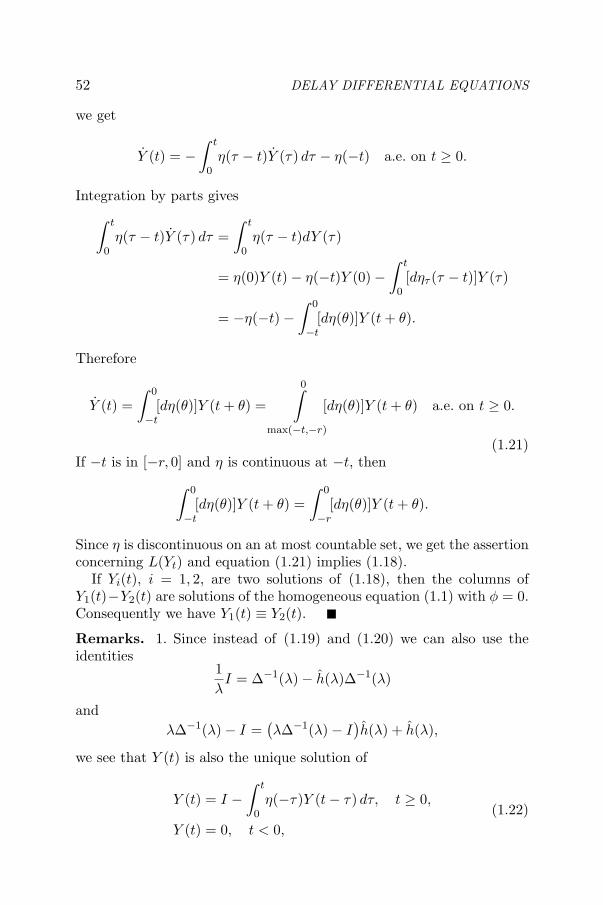
52 DELAY DIFFERENTIAL EQUATIONS
we get
Y (t) = −∫ t
0η(τ − t)Y (τ) dτ − η(−t) a.e. on t ≥ 0.
Integration by parts gives∫ t
0η(τ − t)Y (τ) dτ =
∫ t
0η(τ − t)dY (τ)
= η(0)Y (t) − η(−t)Y (0) −∫ t
0[dητ (τ − t)]Y (τ)
= −η(−t) −∫ 0
−t[dη(θ)]Y (t + θ).
Therefore
Y (t) =∫ 0
−t[dη(θ)]Y (t + θ) =
0∫
max(−t,−r)
[dη(θ)]Y (t + θ) a.e. on t ≥ 0.
(1.21)If −t is in [−r, 0] and η is continuous at −t, then
∫ 0
−t[dη(θ)]Y (t + θ) =
∫ 0
−r[dη(θ)]Y (t + θ).
Since η is discontinuous on an at most countable set, we get the assertionconcerning L(Yt) and equation (1.21) implies (1.18).
If Yi(t), i = 1, 2, are two solutions of (1.18), then the columns ofY1(t)−Y2(t) are solutions of the homogeneous equation (1.1) with φ = 0.Consequently we have Y1(t) ≡ Y2(t).
Remarks. 1. Since instead of (1.19) and (1.20) we can also use theidentities
1λ
I = ∆−1(λ) − h(λ)∆−1(λ)
andλ∆−1(λ) − I =
(λ∆−1(λ) − I
)h(λ) + h(λ),
we see that Y (t) is also the unique solution of
Y (t) = I −∫ t
0η(−τ)Y (t − τ) dτ, t ≥ 0,
Y (t) = 0, t < 0,
(1.22)

Autonomous Functional Differential Equations 53
and
Y (t) =∫ 0
−rY (t + θ)dη(θ) a.e. on t ≥ 0,
Y (0) = I and Y (t) = 0 on t < 0.(1.23)
2. Instead of applying Theorem A.9 to H(λ) we could also proceed asfollows. We write
H(λ) =1λ
∫ 0
−reλθdη(θ) +
∞∑j=2
h(λ)j .
The first term is a Laplace-transform by Lemma 1.6, the Laplace-integralconverging absolutely for Reλ > 0. Using (1.12) we get, for any α > 0,the estimate
∞∑j=2
|h(λ)|j ≤∞∑
j=2
(K
|λ|)j
=K2
|λ|(|λ| − K)
for Re λ ≥ α and |λ| > K. This proves that the assumptions of The-orem A.8 are satisfied. Therefore H(λ) is a Laplace-transform of somefunction H(t). As before we get (1.16). We decided to use Theorem A.9for the proof of Theorem 1.5, because this in addition provided us anexplicit representation of Y (t) in terms of the matrix η.
3. For the proof of Theorem 1.5, b) one could also use Theorem A.6 onconvolutions and just differentiate equation (1.17). This gives
0 = Y (t) +∫ t
0Y (t − τ)η(−τ) dτ + η(−t)
= Y (t) +∫ 0
−t[dY (t + τ)]η(τ) + η(−t)
= Y (t) −∫ 0
−tY (t + τ) dη(τ) = Y (t) −
∫ 0
−rYt(θ) dη(θ)
a.e. on t ≥ 0, which is equation (1.23). If we start with (1.22) we get(1.18).
In analogy to the theory of ordinary differential equations we intro-duce the following notions:
Definition 1.8 The matrix ∆(λ) and the function det ∆(λ) are calledthe characteristic matrix and the characteristic function of equa-tion (1.1), respectively. Y (t) is called the fundamental matrix of(1.1).
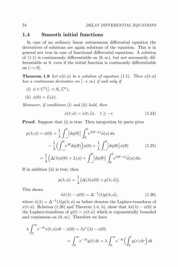
54 DELAY DIFFERENTIAL EQUATIONS
1.4 Smooth initial functionsIn case of an ordinary linear autonomous differential equation the
derivatives of solutions are again solutions of the equation. This is ingeneral not true in case of functional differential equations. A solutionof (1.1) is continuously differentiable on [0,∞), but not necessarily dif-ferentiable at 0, even if the initial function is continously differentiableon [−r, 0].
Theorem 1.9 Let x(t; φ) be a solution of equation (1.1). Then x(t; φ)has a continuous derivative on [−r,∞) if and only if
(i) φ ∈ C1([−r, 0], Cn),
(ii) φ(0) = L(φ).
Moreover, if conditions (i) and (ii) hold, then
x(t; φ) = x(t; φ), t ≥ −r. (1.24)
Proof. Suppose that (i) is true. Then integration by parts gives
p(λ; φ) = φ(0) +1λ
∫ 0
−r
[dη(θ)
] ∫ 0
θeλ(θ−u)φ(u) du
− 1λ
(∫ 0
−reλθdη(θ)
)φ(0) +
1λ
∫ 0
−r
[dη(θ)
]φ(θ)
=1λ
(∆(λ)φ(0) + L(φ) +
∫ 0
−r
[dη(θ)
] ∫ 0
θeλ(θ−u)φ(u) du.
(1.25)
If in addition (ii) is true, then
p(λ; φ) =1λ
(∆(λ)φ(0) + p(λ; φ)
).
This showsλx(λ) − φ(0) = ∆−1(λ)p(λ; φ), (1.26)
where x(λ) = ∆−1(λ)p(λ; φ) as before denotes the Laplace-transform ofx(t; φ). Relation (1.26) and Theorem 1.4, b), show that λx(λ) − φ(0) isthe Laplace-transform of y(t) = x(t; φ) which is exponentially boundedand continuous on (0,∞). Therefore we have
λ
∫ ∞
0e−λtx(t; φ) dt − φ(0) = λx∗(λ) − φ(0)
=∫ ∞
0e−λty(t) dt = λ
∫ ∞
0e−λt
(∫ t
0y(τ) dτ
)dt

Autonomous Functional Differential Equations 55
for Re λ sufficiently large, which implies (note that x(t; φ) is continuous)
x(t; φ) − φ(0) =∫ t
0y(τ) dτ, t ≥ 0.
This shows that x(t; φ) has a continuous derivative on [0,∞). On theother hand relation (1.26) shows that
y(t) = x(t; φ) a.e. on [0,∞).
Since solutions of equation (1.8) are continuous on [−r,∞), this provesthat x(t; φ) has a continuous derivative on [−r,∞) and
x(t; φ) = x(t; φ), t ≥ −r.
Now suppose that x(t; φ) exists on [−r,∞) and is continuous. Thisimplies φ ∈ C1([−r, 0], Rn), of course. By continuity of x(t; φ) at t = 0we get φ(0) = x(0−; φ) = x(0+;φ) = L(φ).
Remarks. 1. Conditions (i) and (ii) characterize the domain of theinfinitesimal generator A corresponding to the solution semigroup T (t),t ≥ 0, associated with equation (1.1) (see Theorem 1.23).2. Since Aφ = φ for φ ∈ domA, relation (1.24) means
AT (t)φ = T (t)Aφ, t ≥ 0, φ ∈ domA,
which is well known for C0-semigroups.
1.5 The variation of constants formulaIn this section we prove a representation formula for x(t; φ) resp.
x(t; φ, f) in terms of the fundamental matrix and the data η, φ andf .
Lemma 1.10 The function
g(λ) = −∫ 0
−r[dη(θ)]
(e0(λ) ∗ φ
)(θ), λ ∈ C,
is the Laplace-transform of the function
g(t) =
∫ −t
−r[dη(θ)]φ(t + θ) for 0 ≤ t ≤ r,
0 for t > r.
If we extend the definition of φ by φ(t) = 0 for t > 0, then
g(t) = L(φt) =∫ 0
−r[dη(θ)]φ(t + θ) (1.27)

56 DELAY DIFFERENTIAL EQUATIONS
for all t ≥ 0 with the exception of an at most countable subset of [0, r](in fact the subset where η(−θ) is discontinuous).
Proof. The representation (1.27) of g follows from the fact that, forφ(0) = 0 and 0 ≤ t ≤ r,
∫ −t
−r[dη(θ)]φ(t + θ) =
∫ 0
−r[dη(θ)]φ(t + θ)
provided η is continuous at −t. If φ(0) = 0, then (1.27) holds for allt ≥ 0.
Using Fubini’s theorem we get
−∫ 0
−r[dη(θ)]
(e0(λ) ∗ φ
)(θ) =
∫ 0
−r[dη(θ)]
∫ −θ
0e−λτφ(τ + θ) dτ
=∫ r
0e−λτ
∫ −τ
−r[dη(θ)]φ(τ + θ) dτ =
∫ ∞
0e−λτg(τ) dτ.
Theorem 1.11 (Variation of Constants Formula) The solution ofproblem (1.1), (1.2) is given by
x(t; φ) = Y (t)φ(0) +∫ t
0Y (t − τ)L(φτ ) dτ, t ≥ 0, (1.28)
where L(φτ ) is defined in Lemma 1.10. The upper limit of the integralcan be replaced by min(t, r).
Proof. The Laplace-transform of x(t; φ) is given by
x(λ) = ∆−1(λ)p(λ; φ) = ∆−1(λ)φ(0) − ∆−1(λ)∫ 0
−r[dη(θ)]
(e0(λ) ∗ φ
)(θ).
From this (1.28) follows by using Lemma 1.10. For the application of theconvolution theorem (Theorem A.7) we have to note that the Laplace-integrals of Y (t) and L(φt) are absolutely convergent in some right halfplane.
For fixed t ≥ 0, φ →∫ t0Y (t − τ)L(φτ ) dτ defines a bounded linear
functional C → Cn, which according to Riesz’ theorem must have a
representation∫ 0−r[dθΦ(θ, t)]φ(θ), where Φ(θ, t), for fixed t ≥ 0, is a
function of bounded variation in θ.
Proposition 1.12 For any φ ∈ C we have∫ t
0Y (t − τ)L(φτ ) dτ =
∫ 0
−r[dθΦ(θ, t)]φ(θ),

Autonomous Functional Differential Equations 57
where
Φ(θ, t) =∫ t
0Y (t − σ)η(θ − σ) dσ, −r ≤ θ ≤ 0, t ≥ 0.
Proof. In order to get the explicit expression for Φ(θ, t) we apply thenon-symmetric Fubini theorem by Cameron and Martin ([6], see alsoTheorem C.1) to the integral
∫ t
0Y (t − τ)L(φτ ) dτ =
t∫
max(0,t−r)
0∫
t−r−σ
[dτη(σ − t + τ)]φ(τ) dσ.
We define the functions
k(σ) =
∫ σ0 Y (τ) dτ for max(0, t − r) ≤ σ ≤ t,
k(t) for σ ≥ t,k(max(0, t − r)) for σ ≤ max(0, t − r),
s(τ) =
φ(τ) for −r ≤ τ ≤ 0,0 for τ > 0,
φ(−r) for τ ≤ −r,
p(σ, τ) = η(σ − t + τ) for σ, τ ∈ R.
We also change, for this proof the definition of η at points of discontinuityin [−r, 0) such that η is right-hand continuous on R. Then we have∫ t
0Y (t − τ)L(φτ ) dτ =
∫ ∞
−∞
[∫ ∞
−∞s(τ)dτp(σ, τ)
]dk(σ).
It is clear that the function s(τ) is Borel-measurable on R, k is ofbounded variation on bounded intervals and τ → p(σ, τ) is of boundedvariation on bounded intervals for all σ ∈ R. Borel-measurability of p onR
2 follows from Borel-measurability of the mappings (σ, τ) → σ + τ − ton R
2 and η on R. In order to verify condition (i) of Theorem C.1 wehave to investigate
V (σ, τ) =∫ τ
0
∣∣dνp(σ, ν)∣∣ =
∫ σ−t+τ
σ−t|dη(θ)| = var[σ−t,σ−t+τ ]η for τ ≥ 0,
V (σ, τ) = −∫ τ
0
∣∣dνp(σ, ν)∣∣ = −var[σ−t+τ,σ−t]η for τ < 0.
By definition of k we get
∫ ∞
−∞V (σ, τ)|dk(σ)| =
t∫
max(0,t−r)
V (σ, τ)|Y (σ)| dσ < ∞, t ∈ R.

58 DELAY DIFFERENTIAL EQUATIONS
This shows that condition (i) of Theorem C.1 holds. We also have∫ ∞
−∞|s(τ)| |dτp(σ, τ)| ≤ ‖φ‖var[−r,0]η, σ ∈ R,
and∫ ∞
−∞
∫ ∞
−∞|s(τ)| |dτp(σ, τ)| |dk(σ)|
≤ ‖φ‖var[−r,0]η
t∫
max(0,t−r)
|Y (τ)| dτ < ∞,
i.e., also condition (ii) of Theorem C.1 is satisfied. Therefore we get∫ t
0Y (t − τ)L(φτ ) dτ =
∫ ∞
−∞
[dτ
∫ ∞
−∞[dk(σ)]p(σ, τ)
]s(τ)
=∫ 0
−r
[dτ
t∫
max(0,t−r)
Y (σ)η(σ − t + τ) dσ]φ(τ).
This proves
Φ(θ, t) =
t∫
max(0,t−r)
Y (σ)η(σ − t + θ) dσ =
min(t,r)∫
0
Y (t − σ)η(θ − σ) dσ
for −r ≤ θ ≤ 0 and t ≥ 0. The upper limit min(t, r) in the second inte-gral can be replaced by t. One easily checks that the resulting functionΦ(θ, t) would differ only by a constant, which does not matter.
We next turn to the nonhomogeneous problem (1.3), (1.4). If is suffi-cient to consider the case φ = 0 only. For any t1 > 0 we define
f(t; t1) =
f(t) for 0 ≤ t ≤ t1,0 for t > t1.
Instead of equation (1.3) we consider for the moment
x(t) = L(xt) + f(t; t1), t ≥ 0. (1.29)
The estimates (1.8) and (1.9) imply
|x(t; 0, f(·; t1))| ≤∫ t1
0|f(τ)| dτ et, t ≥ 0,
|x(t; 0, f(·; t1))| ≤
∫ t1
0|f(τ)| dτ et, t ≥ 0.

Autonomous Functional Differential Equations 59
Therefore the Laplace-transforms of x(t) = x(t; 0, f(·, t1)) and x(t) ex-ist, the Laplace-integrals converging absolutely for Reλ > . TakingLaplace-transforms on both sides of equation (1.29) we get
x(λ) = ∆−1(λ)f(λ; t1), (1.30)
where f(λ; t1) =∫ t10 e−λtf(t) dt. This implies
x(t) =∫ t
0Y (t − τ)f(τ ; t1) dτ, t ≥ 0.
Since x(t; 0, f(·, t1)) = x(t; 0, f) for 0 ≤ t ≤ t1 and t1 > 0 was arbitrary,we have proved the following theorem:
Theorem 1.13 For any φ ∈ C and f ∈ L1loc(0,∞; Cn), the solution of
problem (1.3), (1.4) is given by
x(t; φ, f) = x(t; φ) +∫ t
0Y (t − τ)f(τ) dτ, t ≥ 0. (1.31)
Remark. Theorem 1.7, b) implies that, for any a ∈ Cn, the function
x(t; a) = Y (t)a, t ≥ −r, is the unique solution of
x(t) = L(xt) a.e. on t ≥ 0,x(0) = a and x(t) = 0 for −r ≤ t < 0.
(1.32)
Therefore formula (1.28) can be viewed as the variation of constantsformula for the nonhomogeneous problem
x(t) = L(xt) + f(t) a.e. on t ≥ 0,x(0) = a and x(t) = 0 for −r ≤ t < 0,
(1.33)
where a = φ(0) and f(t) = L(φt), t ≥ 0.Formula (1.28) also shows that the solution x(t; φ) is the sum of two
functions. One is the solution of (1.32) with a = φ(0) and therefore isinfluenced only by φ(0), the other is the solution of (1.33) with a = 0and f(t) = L(φt) and depends only on the past history φ |[−r,0).
1.6 The SpectrumAs we have seen in Section 1.3 the Laplace-integral for any solution
x(t) = x(t; φ) of (1.1), (1.2) is absolutely convergent for Reλ > (seeProposition 1.4). Therefore the complex inversion formula (cf. Theo-rem A.10) is applicable for any γ > and gives
x(t; φ) =∫
(γ)
eλt∆−1(λ)p(λ; φ) dλ, t > 0. (1.34)

60 DELAY DIFFERENTIAL EQUATIONS
For t = 0 the integral gives12φ(0) and zero for t < 0. Here and in the
following we use the notation∫
(γ)
f(λ) dλ =1
2πilim
T→∞
∫ T
−Tf(γ + iτ) dτ.
We shall show in the next section that instead of taking γ > in (1.34)we can choose any γ > supRe λ | ∆−1(λ)p(λ; φ) has a pole at λ. Sincethe poles of ∆−1(λ)p(λ; φ) occur under the zeros of det ∆(λ), we shallinvestigate first the location of these zeros.
Definition 1.14 The set σ(L) = λ ∈ C | det ∆(λ) = 0 is called thespectrum of equation (1.1) and ρ(L) = C \ σ(L) is the resolvent setof equation (1.1).
We first state some basic facts about σ(L):
Proposition 1.15 a) σ(L) is non-empty and all points of σ(L) are iso-lated in C. If σ(L) is finite, then det∆(λ) is a polynomial in λ of degreen.
b) If λ0 ∈ σ(L)is a zero of det ∆(λ) with multiplicity k0, then λ0 is poleof some order κ0 for ∆−1(λ) (i.e., λ0 is pole of at least one element of∆−1(λ) and κ0 is the maximal order occuring). Moreover, we have
0 < κ0 ≤ k0.
c) There exists a constant ρ > 0 such that (see the shaded areas inFigure 1)
σ(L) ⊂ λ | Re λ ≥ 0 and |λ| ≤ ρ ∪ λ | Re λ < 0 and |λ|ern Re λ ≤ ρ.

Autonomous Functional Differential Equations 61
Proof. a) Since det∆(λ) is an entire function, the elements of σ(L)are isolated points and zeros of finite multiplicity. Let λ0 ∈ σ(L) be
a zero of multiplicity k0. From ∆−1(λ) =1
det∆(λ)adj∆(λ) it is clear
that λ0 is a pole of order κ0 ≤ k0, because the elements of adj∆(λ) areentire functions. We have to prove that λ0 is indeed a pole for ∆−1(λ).Suppose that ∆−1(λ) is holomorphic at λ0. Then this is also true fordet ∆−1(λ) and det ∆(λ) det ∆−1(λ). This leads to the contradiction0 = det ∆(λ0) det ∆−1(λ0) = limλ→λ0 det ∆(λ) det ∆−1(λ) = 1.
b) We may write
det ∆(λ) = λn + αn−1(λ)λn−1 + · · · + α1(λ)λ + α0(λ), (1.35)
where each αk(λ) is a finite sum of products of at most n of the functions∫ 0−re
λθdηij(θ), i, j = 1, . . . , n. The estimate (1.11) therefore implies thatthere exists a constant δ > 0 such that
|αk(λ)| ≤
δ for Re λ ≥ 0,e−rn Re λδ for Re λ < 0,
(1.36)
k = 0, . . . , n − 1. Therefore we have the estimates
|det∆(λ)| ≥ |λ|n(1 − δ
n∑k=1
|λ|−k)
for Re λ ≥ 0
and
|det∆(λ)| ≥ |λ|n(1 − δ
n∑k=1
e−rn Re λ|λ|−k)
≥ |λ|n(1 − δ
n∑k=1
(ern Re λ|λ|
)−k) for Re λ < 0.
Note that e−n Re λ > 1 for Reλ < 0. If |λ| > ρ for Re λ ≥ 0 and|λ|ern Re λ > ρ for Re λ < 0 with ρ > 0 satisfying
∑nk=1 ρ−k = 1/δ, then
|det∆(λ)| > 0. If we set λ = µ + iν, µ, ν real, then we have
ν = ±ρe−rnµ(1 − µ2
ρ2e2rnµ
)1/2, µ < 0,
for |λ|ern Re λ = ρ. In Figure 1 we show this curve for ρ = 1 and r = .5resp. r = .35. We also see that ν behaves like ±ρe−rnµ as µ → −∞.

62 DELAY DIFFERENTIAL EQUATIONS
c) It remains to prove the result for finite σ(L). Suppose that σ(L) isempty or finite. Using (1.36) and the representation (1.35) for det∆(λ)we get
|det ∆(λ)| ≤(|λ|n + · · · + |λ| + 1
)ern|λ|
for λ ∈ C, which shows that det∆(λ) is a function of exponential type(see Definition B.1). Therefore the assumption on σ(L) implies (cf.Theorem B.7)
det ∆(λ) = p(λ)eαλ,
where p(λ) is a polynomial of degree ≥ 0 and α ∈ C. Taking absolutevalues we get
eRe(αλ) =|det∆(λ)|
|p(λ)| , λ /∈ σ(L).
This together with (1.36) implies
(|λ|n−δ
n−1∑j=0
|λ|j)|p(λ)|−1 ≤ eRe(αλ) ≤
(|λ|n+δ
n−1∑j=0
|λ|j)|p(λ)|−1 (1.37)
for Re λ ≥ 0 and |λ| sufficiently large. With σ = arg α we choose λk =keiζk where ζk = −σ + π/2 or ζk = −σ − π/2 such that Re(αλk) = 0and Reλk ≥ 0. For k → ∞ we see that (1.37) is only possible if p(λ)is a polynomial of degree n. Therefore σ(L) is not empty. Suppose α isnot real. Then (1.37), for λ = iω, ω real, gives
e−ω Im α ≤(|ω|n + δ
n−1∑j=0
|ω|j) 1|p(iω)| .
The right-hand side of this inequality is bounded for |ω| ≥ n0, n0 suffi-ciently large, whereas the left-hand side is not. Thus α has to be real.But (1.37) implies that
limρ→∞
eαρ =1
|pn|,
where pn = 0 is the coefficient of λn in p(λ). Thus we have α = 0 andpn = 1.
Define the matrix η0 = (η0ij) by η0(θ) = η(θ) for θ < 0 and by η0(0) =
η(0−). We set A0 = −η(0−). Then∫ 0
−reλθdη(θ) = A0 +
∫ 0
−reλθdη0(θ).
In view of Proposition 1.15, a), the question arises if det ∆(λ) = det(λI−A0) provided σ(L) is finite. We can prove this under an additionalassumption on η:

Autonomous Functional Differential Equations 63
Proposition 1.16 Assume that there exists a δ > 0 such that η0(θ) =η0(−δ) for θ ∈ [−δ, 0]. If σ(L) is finite, then
det ∆(λ) = det(λI − A0).
Proof. The coefficients αj(λ) in (1.35) can be written as
αj(λ) = aj + βj(λ), j = 0, . . . , n − 1, (1.38)
where the aj are the coefficients of det(λI −A0) and the βj(λ) are finitesums of finite products involving elements of A0 and of
∫ 0−re
λθdη0(θ).In each product at least one factor is of the form
∫ 0−re
λθdη0ij(θ). The
assumption on η0 implies∣∣∣∫ 0
−reρθdη0
ij(θ)∣∣∣ ≤ e−ρδvar[−r,0]η
0ij , i, j = 1, . . . , n, ρ > 0. (1.39)
From
q(λ) = βn−1(λ)λn−1 + · · · + β1(λ)λ + β0(λ) = det ∆(λ) − det(λI − A0)
we see that q(λ) is a polynomial of degree ≤ n − 1. On the other handthe estimate (1.39) implies that, for a constant K > 0,
|q(ρ)| ≤ Ke−ρδρn−1 for ρ ≥ 1.
This implies that q(λ) is the zero polynomial.An immediate and important consequence of Proposition 1.15, c),
and the fact that σ(L) cannot have an accumulation point in C is thefollowing result:
Corollary 1.17 For any α ∈ R the set
σ(L) ∩ λ ∈ C | Re λ ≥ α
is finite.
We shall need the following estimates:
Lemma 1.18 Let α ∈ R be given. Then the following is true:
a) There exist positive constants K = K(α) and β = β(α) such that
|∆−1(λ)| ≤ K
|λ| for |λ| ≥ β and Re λ ≥ α.
b) There exists a positive constant M = M(α) such that
|p(λ; φ)| ≤ M‖φ‖ for Re λ ≥ α and φ ∈ C.
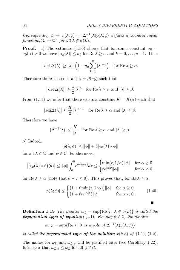
64 DELAY DIFFERENTIAL EQUATIONS
Consequently, φ → x(λ; φ) = ∆−1(λ)p(λ; φ) defines a bounded linearfunctional C → C
n for all λ ∈ σ(L).
Proof. a) The estimate (1.36) shows that for some constant σ0 =σ0(α) > 0 we have |αk(λ)| ≤ σ0 for Re λ ≥ α and k = 0, . . . , n−1. Then
|det∆(λ)| ≥ |λ|n(1 − σ0
n∑k=1
|λ|−k)
for Re λ ≥ α.
Therefore there is a constant β = β(σ0) such that
|det∆(λ)| ≥ 12|λ|n for Re λ ≥ α and |λ| ≥ β.
From (1.11) we infer that there exists a constant K = K(α) such that
|adj∆(λ)| ≤ K
2|λ|n−1 for Re λ ≥ α and |λ| ≥ β.
Therefore we have
|∆−1(λ)| ≤ K
|λ| for Re λ ≥ α and |λ| ≥ β.
b) Indeed,|p(λ; φ)| ≤ ‖φ‖ + ‖e0(λ) ∗ φ‖
for all λ ∈ C and φ ∈ C. Furthermore,
∣∣(e0(λ) ∗ φ)(θ)∣∣ ≤ ‖φ‖
∫ 0
θeα(θ−τ)dτ ≤
min(r, 1/α)‖φ‖ for α ≥ 0,re|α|r‖φ‖ for α < 0,
for Re λ ≥ α (note that θ − τ ≤ 0). This proves that, for Reλ ≥ α,
|p(λ; φ)| ≤(
1 + min(r, 1/α))‖φ‖ for α ≥ 0,(
1 + re|α|r)‖φ‖ for α < 0.
(1.40)
Definition 1.19 The number ωL = supRe λ | λ ∈ σ(L) is called theexponential type of equation (1.1). For any φ ∈ C, the number
ωL,φ = supRe λ | λ is a pole of ∆−1(λ)p(λ; φ)
is called the exponential type of the solution x(t; φ) of (1.1), (1.2).
The names for ωL and ωL,φ will be justified later (see Corollary 1.22).It is clear that ωL,φ ≤ ωL for all φ ∈ C.

Autonomous Functional Differential Equations 65
Proposition 1.20 a) For any γ > ωL,
Y (t) =∫
(γ)
eλt∆−1(λ) dλ for t > 0. (1.41)
b) For any γ > ωL,φ,
x(t; φ) =∫
(γ)
eλt∆−1(λ)p(λ; φ) dλ for t > 0. (1.42)
Proof. We only prove part b). According to the definition of ωL,φ wehave for all T > 0 ∫
Γ
eλt∆−1(λ)p(λ; φ) dλ = 0, (1.43)
where Γ is the closed contour depicted in Figure 2.
Of course, we have ωL,φ < γ ≤ γ0 and < γ0. By Lemma 1.18 thereexist positive constants K and ρ such that
∣∣eλt∆−1(λ)p(λ; φ)∣∣ ≤ K
|λ|
for γ ≤ Re λ ≤ γ0 and | Im λ| ≥ ρ. This shows
limT→∞
∫
Γi
eλt∆−1(λ)p(λ; φ) dλ = 0, i = 1, 2, (1.44)

66 DELAY DIFFERENTIAL EQUATIONS
where Γ1 and Γ2 are the horizontal parts of Γ (see Figure 2). By choice ofγ0, the Laplace-integral for x(t; φ) is absolutely convergent for Reλ ≥ γ0
and therefore (cf. Theorem A.10)
x(t; φ) =∫
(γ0)
eλt∆−1(λ)p(λ; φ) dλ, t > 0.
By (1.43) and (1.44) also∫(γ) eλt∆−1(λ)p(λ; φ) dλ exists and equals x(t; φ)
for t > 0. This proves (1.42).In the proof concerning Y (t) we have to choose γ0 > β, where β is
the number appearing in Theorem 1.5.We now are able to prove that the numbers ωL and ωL,φ determine
the exponential growth of Y (t) and x(t;φ), respectively.
Theorem 1.21 a) The number ωL is the smallest number such that forany ε > 0 there exists a constant K = K(ε) ≥ 1 such that
|Y (t)| ≤ Ke(ωL+ε)t for t ≥ 0. (1.45)
b) The number ωL,φ is the smallest number such that for any ε > 0there exists a constant K = K(ε) ≥ 1 such that for any ψ ∈ C withωL,ψ ≤ ωL,φ
|x(t; ψ)| ≤ K‖ψ‖e(ωL,φ+ε)t for t ≥ 0. (1.46)
There always exists a φ ∈ C such that ωL,φ = ωL.
Proof. Again we just prove b). We show first that ωL,φ cannot bereplaced by a smaller number. Indeed, assume that (1.46) is true fora γ < ωL,φ. Then, for ε = (ωL,φ − γ)/2 we have γ + ε < ωL,φ and|x(t; φ)| ≤ K(ε)‖φ‖e(γ+ε)t, t ≥ 0, which implies that the Laplace-integralfor x(t; φ) converges absolutely for Re λ > γ, a contradiction to thedefinition of ωL,φ.
We now choose a ψ ∈ C with ωL,ψ ≤ ωL,φ. For ε > 0 we set ωL,φ+ε = γand get from (1.42)
x(t; ψ) =∫
(γ)
eλt∆−1(λ)p(λ; ψ) dλ, t > 0.
According to the identity
∆−1(λ)p(λ; ψ) =(∆−1(λ)−(λ−ωL,φ)−1I
)p(λ; ψ)+(λ−ωL,φ)−1p(λ; ψ)
= (λ − ωL,φ)−1∆−1(λ)(−ωL,φI +
∫ 0
−reλθdη(θ)
)p(λ; ψ)
+ (λ − ωL,φ)−1p(λ; ψ)

Autonomous Functional Differential Equations 67
we have to estimate
I1 =∫
(γ)
eλt(λ − ωL,φ)−1∆−1(λ)(−ωL,φI +
∫ 0
−reλθdη(θ)
)p(λ; ψ) dλ
and
I2 =∫
(γ)
eλt(λ − ωL,φ)−1p(λ; ψ) dλ.
By Lemma 1.18 and (1.11) there exist positive constants K = K(γ),M = M(γ), N = N(γ) and β such that for λ = γ + iτ
∣∣eλt(λ − ωL,φ)−1∆−1(λ)(−ωL,φI +
∫ 0
−reλθdη(θ)
)p(λ; ψ)
∣∣
≤ eγt 1|τ |
K
|τ |(|ωL,φ| + N
)M‖ψ‖ =
K
τ2‖ψ‖eγt, |τ | ≥ β.
This implies that|I1| ≤ κ1‖ψ‖ eγt, t > 0, (1.47)
where κ1 = κ1(γ) is some positive constant. With respect to I2 we ob-serve that (λ − ωL,φ)−1ψ(0) is the Laplace-transform of eωL,φtψ(0) and−(λ − ωL,φ)−1L(e0(λ) ∗ ψ) is the Laplace-transform of the convolutioneωL,φt∗L(ψt) (see Lemma 1.10). All Laplace-integrals are converging ab-solutely for Reλ > ωL,φ. For eωL,φt this is trivial and for the convolutionit is valid because it is true for both factors. Therefore we have
I2 = ψ(0)eωL,φt +∫ t
0eωL,φ(t−τ)L(ψτ ) dτ, t ≥ 0.
For the integral we get (note that L(ψτ ) = 0 for τ > r)
∣∣∣∫ t
0eωL,φ(t−τ)L(ψτ ) dτ
∣∣∣ ≤min(t,r)∫
0
eωL,φ(t−τ)|L(ψτ )| dτ
≤ eωL,φt
∫ r
0|L(ψτ )| dτ ≤ κ2e
ωL,φt‖ψ‖,
where κ2 is a positive constant which does not depend on ψ. Thereforewe get
|I2| ≤ eωL,φt‖ψ‖(1 + κ2) for t ≥ 0. (1.48)
Since x(t; ψ) = I1 + I2, the desired result follows from (1.47) and (1.48).

68 DELAY DIFFERENTIAL EQUATIONS
An easy calculation shows that x(t) = eλ0tb is a nontrivial solution ofequation (1.1) if and only if det ∆(λ0) = 0 and b is a nonzero solution of∆(λ0)b = 0. Therefore, for any λ0 ∈ σ(L), we have at least one solutionwhose exponential type is Reλ0 (note that L(eλ0t) = (λ − λ0)−1).
Corollary 1.22 We have
lim supt→∞
1t
ln |Y (t)| = ωL
and, for any φ ∈ C,
lim supt→∞
1t
ln |x(t; φ)| = ωL,φ.
The proof of this corollary is an immediate consequence of Theorem 1.21.
1.7 The solution semigroupFor any t ≥ 0 we define the operator T (t) : C → C by
T (t)φ = xt(φ), φ ∈ C.
From Proposition 1.3 (for f ≡ 0) we see that T (t) is a bounded linearoperator. Since xt+s(φ) = xt(xs(φ)) for t, s ≥ 0, we also have
T (t + s) = T (t)T (s), t, s ≥ 0,
i.e., the family T =(T (t)
)t≥0
is a semigroup. Since x(t; φ) is uniformlycontinuous on intervals [−r, T ], T ≥ −r, it is clear that
‖xt(φ) − φ‖ = sup−r≤θ≤0
|x(t + θ; φ) − φ(θ)| → 0 as t ↓ 0,
which proves that S is a C0-semigroup.
Theorem 1.23 a) The infinitesimal generator A of S is given by
domA = φ ∈ C1(−r, 0; Cn) | φ′(0) = L(φ),Aφ = φ′, φ ∈ domA.
(1.49)
b) The spectrum σ(A) of A is all point spectrum and is given by
σ(A) = σ(L) = λ ∈ C | det ∆(λ) = 0.
c) The resolvent operator of A is given by
ψλ = (λI −A)−1φ, φ ∈ C,

Autonomous Functional Differential Equations 69
where
ψλ(θ) = ψλ(0)eλθ +∫ 0
θeλ(θ−s)φ(s) ds,
ψλ(0) = ∆(λ)−1p(λ; φ) = x(λ; φ).
Proof. We first compute the resolvent operator for the operator definedby (1.49). The equation (λI − A)ψλ = φ, φ ∈ C, ψλ ∈ domA, impliesψ′
λ(θ) = λψλ(θ) − φ(θ), −r ≤ θ ≤ 0, and
ψλ(θ) = ψλ(0)eλθ +∫ 0
θeλ(θ−s)φ(s) ds, −r ≤ θ ≤ 0.
The function ψλ is in C1(−r, 0; Cn). We have to choose ψλ(0) such thatψλ ∈ domA, i.e.,
λψλ(0) − φ(0) = L(ψλ) = L(eλ·I)ψλ(0) + L(∫ 0
·eλ(·−s)φ(s) ds
)
or, equivalently,
∆(λ)ψλ(0) = φ(0) + L(∫ 0
·eλ(·−s)φ(s) ds
)= p(λ; φ).
This equation can be solved for ψλ(0) if and only if det ∆(λ) = 0. Inthis case we have
ψλ(0) = ∆(λ)−1p(λ; φ) = x(λ; φ).
From Lemma 1.18, b) we see that φ → ψλ(0) defines a bounded linearfunctional C → C
n. This implies that φ → ψλ is a bounded linearoperator C → C. Therefore we have shown that λ ∈ σ(A) if and only ifdet ∆(λ) = 0. Moreover, λ ∈ σ(A) implies that λI − A is not injective((λI−A)ψ = 0, ψ ∈ domA, is equivalent to ψ(θ) = ψ(0)eλθ, −r ≤ θ ≤ 0,and ∆(λ)ψ(0) = 0). Thus parts b) and c) are proved.
It remains to prove that A is the infinitesimal generator of T . Forthe moment let B denote the infinitesimal generator of T . Then we have(see for instance [28])
(λI − B)−1φ =∫ ∞
0e−λtT (t)φdt, φ ∈ C, Re λ > ωL,

70 DELAY DIFFERENTIAL EQUATIONS
where the integral is understood as an improper Riemann integral. Onthe other hand a simple integration using also part c) shows that(∫ ∞
0e−λtT (t)φ dt
)(θ) =
(∫ ∞
0e−λtxt(φ) dt
)(θ) =
∫ ∞
0e−λtx(t + θ; φ) dt
=∫ 0
θeλ(θ−s)φ(s) ds + eλθ
∫ ∞
0eλtx(t; φ) dt
= x(λ; φ)eλθ +∫ 0
θeλ(θ−s)φ(s) ds
=((λI −A)−1φ
)(θ), −r ≤ θ ≤ 0, Re λ > ωL.
This proves (λI −A)−1 = (λI − B)−1, Re λ > ωL, i.e., A = B.For the proof of A = B we have also used the following lemma:
Lemma 1.24 For any θ ∈ [−r, 0] we have(∫ ∞
0e−λtxt(φ) dt
)(θ) =
∫ ∞
0e−λtx(t + θ; φ) dt, Re λ > ωL.
Proof. Let m be a bounded linear functional on C which is representedby the vector µ of bounded variation on [−r, 0],
m(φ) =∫ 0
−rφ(θ)dµ(θ), φ ∈ C.
Then we have
m(∫ ∞
0e−λtxt(φ) dt
)=∫ ∞
0m(e−λtxt(φ)
)dt
=∫ ∞
0
∫ 0
−rx(t + θ; φ) dµ(θ) dt.
It is not difficult to prove that θ →∫∞0 e−λtx(t + θ; φ) dt, −r ≤ θ ≤ 0, is
a function in C. Using Fubini’s theorem we get
m(∫ ∞
0e−λtx(t + θ; φ) dt
)=∫ 0
−r
∫ ∞
0e−λtx(t + θ; φ) dt dµ(θ)
=∫ ∞
0
∫ 0
−re−λtx(t + θ; φ) dµ(θ) dt.
Thus we have shown that
m(∫ ∞
0e−λtxt(φ) dt
)= m
(∫ ∞
0e−λtx(t + ·; φ) dt
)
for all bounded linear functionals m on C, which proves the result.

Autonomous Functional Differential Equations 71
2. Eigenspaces
2.1 Generalized eigenspacesConsider equation (1.1) with
L(φ) =∫ 0
−r[dη(θ)]φ(θ), φ ∈ C.
A function x(t) = eλ0tb0, λ0 ∈ C, b0 ∈ Cn, is a solution of (1.1) if and
only ifdet ∆(λ0) = 0 and ∆(λ0)b0 = 0.
Similarly a function x(t) = eλ0t(b0 + tb1
), λ0 ∈ C, b0, b1 ∈ C
n, is asolution of (1.1) if and only if
t∆(λ0)b1 +(I −
∫ 0
−rθeλ0θdη(θ)
)b1 + ∆(λ0)b0 ≡ 0,
which in turn is equivalent to
∆(λ0)b1 = 0,
∆(λ0)b0 + ∆′(λ0)b1 = 0
(observe that ∆′(λ0) = I −∫ 0−rθe
λ0θdη(θ)). In general we have:
Proposition 2.1 Let λ0 ∈ C and bj ∈ Cn, j = 0, . . . , k, be given. The
function
x(t) = eλ0tk∑
j=0
tj
j!bj ≡ 0 (2.1)
is a solution of (1.1) on R if and only if
(i) λ0 ∈ σ(L),
(ii) ∆k+1(λ0)bk+1 = 0, bk+1 = 0,
where
∆k+1(λ0) =
∆(λ0) 11!∆
′(λ0) · · · · · · 1k!∆
(k)(λ0)
0. . . . . .
......
. . . . . . . . ....
.... . . . . . 1
1!∆′(λ0)
0 · · · · · · 0 ∆(λ0)
∈ Cn(k+1)×n(k+1),
bk+1 = col (b0, . . . , bk) ∈ Cn(k+1).

72 DELAY DIFFERENTIAL EQUATIONS
Definition 2.2 Let λ0 ∈ σ(L) be given. The subspace
Pλ0 =φ ∈ C |∃k ≥ 0 : φ(θ) = eλ0θ
k∑j=0
θj
j!bj , −r ≤ θ ≤ 0,
where ∆k+1(λ0)bk+1 = 0
is called the generalized eigenspace of (1.1) corresponding to λ0. Afunction x(t) given by (2.1) with bk satisfying (ii) of Proposition 2.1 iscalled a generalized eigenfunction of equation (1.1) corresponding toλ0.
For λ0 ∈ σ(L) let k0 be the multiplicity of λ0 as a root of det∆(λ)and κ0 be the order of λ0 as a pole of ∆−1(λ). We know already that
0 < κ0 ≤ k0.
We first show that in the definition of Pλ0 we can set k = κ0 − 1.3
Proposition 2.3 Let λ0 ∈ σ(L) be given.
a) The generalized eigenspace of (1.1) corresponding to λ0 is given by
Pλ0 =φ ∈ C |φ(θ) = eλ0θ
κ0−1∑j=0
θj
j!bj , −r ≤ θ ≤ 0,
where ∆κ0(λ0)bκ0 = 0.
(2.2)
b) dim Pλ0 = nκ0 − rank ∆κ0(λ0).
Proof. a) Assume that, for a φ ∈ Pλ0 , we have k ≥ κ0, i.e.,
φ(θ) = eλ0θk∑
j=0
θj
j!bj , ∆k+1(λ0)bk+1 = 0.
The solution x(t; φ) is given by
x(t; φ) = eλ0tk∑
j=0
tj
j!bj .
The Laplace-transform of x(t; φ) is
x(λ; φ) =k∑
j=0
1(λ − λ0)j+1
bj .
3Below we shall prove that κ0 cannot be replaced by a smaller number (see Corollary 2.9).

Autonomous Functional Differential Equations 73
Since λ0 can be a pole of x(λ; φ) of order at most κ0 (observe thatx(λ; φ) = ∆−1(λ)p(λ; φ)), we must have
bκ0 = bκ0+1 = · · · = bk = 0,
i.e., bk = col(b0, . . . , bκ0−1, 0, . . . , 0). From ∆k+1(λ0)bk+1 = 0 we imme-diately get
∆κ0(λ0)bκ0 = 0.
If φ ∈ Pλ0 is defined with k < κ0 − 1, we define bk+1 = bk+2 = · · · =bκ0−1 = 0. From ∆k+1(λ0)bk+1 = 0 we get that also
∆κ0(λ0)bκ0 = 0.
b) Let φi(θ) = eλ0θ∑κ0−1
j=0θj
j! b(i)j , i = 1, . . . , m, be elements in Pλ0 and
choose α1, . . . . . . , αm ∈ C. The equation∑m
i=1 αiφi = 0 is equivalent to
κ0−1∑j=0
θj
j!
m∑i=1
αib(i)j ≡ 0,
which by linear independence of the functions 1, θ, θ2/2!, . . .. . . , θκ0−1/(κ0 − 1)! is in turn equivalent to
m∑i=1
αib(i)j = 0 for j = 0, . . . , κ0 − 1.
The last equations are equivalent to
m∑i=1
αib(i)κ0
= 0.
This proves that the elements φ1, . . . , φm ∈ Pλ0 are linearly indepen-dent if and only if the vectors b
(1)κ0 , . . . , b
(m)κ0 ∈ ker ∆κ0(λ0) are linearly
independent. The result on dimPλ0 follows immediately.In order to determine rank ∆κ0(λ0) we have to use an elementary
divisor theory for holomorphic matrices. We start with a fundamentaltheorem.
Theorem 2.4 Let K(λ) be an n × n-matrix which is holomorphic in aneighborhood V of zero. If det K(λ) ≡ 0 in V , then there exist integers, dρ, mρ, ρ = 1, . . . , , with
0 ≤ d1 < · · · < d and mρ > 0, ρ = 1, . . . , ,

74 DELAY DIFFERENTIAL EQUATIONS
n × n-matrices F (λ), G(λ) and a neighborhood U of zero such that
(i) M(λ) = F (λ)K(λ)G(λ) = diag(λd1M1(λ), . . . , λdM(λ)
)in U ,
(ii) F (λ), G(λ) are holomorphic in U and det F (λ) ≡ det G(λ) ≡ 1 inU ,
(iii) Mρ(λ), ρ = 1, . . . , , is an mρ × mρ-matrix, which is holomorphicin U with det Mρ(λ) = 0 in U ,
(iv) the numbers , mρ, dρ are uniquely determined by properties (i) –(iii).
Proof. The power series expansion of K(λ) around 0 has the followingform:
K(λ) = λn1H(λ), H0 = 0, n1 ≥ 0,
where H(λ) =∑∞
j=0 λjHj .
Case 1.Assume that det H0 = 0. In this case we have F (λ) ≡ G(λ) ≡ I, = 1,d1 = n1, m1 = n, because
K(λ) = λn1H(λ)
satisfies already (i)–(iii).
Case 2.Assume that det H0 = 0. Let m1 = rank H0. From H0 = 0 and detH0 =0 we see that
0 < m1 < n.
Let X, Y be n × n-matrices with det X = det Y = 1 such that
XH0Y =(
H00 00 0
),
where H00 is an m1 × m1-matrix with detH00 = 0. Observing H(λ) =H0 + λ
∑∞j=1 λj−1Hj we get
XH(λ)Y =(
H00 00 0
)+ λ
(H11(λ) H12(λ)H21(λ) H22(λ)
),
where the Hij(λ) are matrices which are holomorphic in V . We set
M1(λ) = H00 + λH11(λ).

Autonomous Functional Differential Equations 75
From det H00 = 0 we conclude that det M1(λ) = 0 in a neighborhood Uof 0. Therefore M1(λ)−1 exists in U and is holomorphic there. From theequation(
I 0−λH21M
−11 I
)(M1 λH12
λH21 λH22
)(I −λM−1
1 H12
0 I
)=(
M1 00 λK2
),
where K2(λ) = H22(λ) − λH21(λ)M1(λ)−1H12(λ), we see that
F1(λ)K(λ)G1(λ) =(
λn1M1(λ) 00 λn1+1K2(λ)
),
where det F1(λ) ≡ det G1(λ) ≡ 1 in U . The matrix K2(λ) is holomorphicin U and has a power series expansion
K2(λ) = λn2
∞∑j=0
λjH(2)j with H
(2)0 = 0.
If det H(2)0 = 0, then we have
d1 = n1, d2 = n1 + n2 + 1 > d1, m2 = n − m1, = 2
and M2(λ) = K2(λ).If detH
(2)0 = 0, we set m2 = rankH
(2)0 and proceed as above in Case 2.
In a finite number of steps we arrive at M(λ) as given in the theorem.It remains to prove (iv). In order to do this we have to introduce the
notion of determinantal divisors for a holomorphic matrix.For an n×n-matrix N(λ) which is holomorphic in a neighborhood U
of zero we introduce the numbers βν(N), ν = 1, . . . , n, as follows:
(i) Any ν × ν-minor of N(λ) has the form
λβν(N)q(λ), λ ∈ U,
where q(λ) is holomorphic in U .
(ii) There exists at least one ν × ν-minor of N(λ) such that q(0) = 0.
Since a (ν + 1) × (ν + 1)-minor is a linear combination of ν × ν-minors(Laplace expansion theorem for determinants), we have
βν+1(N) ≥ βν(N), ν = 1, . . . , n − 1.
The following lemma shows that equivalence transformations of theform appearing in Theorem 2.4 leave the numbers βν invariant.

76 DELAY DIFFERENTIAL EQUATIONS
Lemma 2.5 Let K(λ) be an n×n-matrix being holomorphic in a neigh-borhood U of 0. Let M(λ) = F (λ)K(λ)G(λ), λ ∈ U , where F (λ) andG(λ) satisfy (ii) of Theorem 2.4. Then we have
βν(M) = βν(K), ν = 1, . . . , n.
Proof. If K(
j1,...,jν
k1,...,kν
)denotes the ν×ν-minor containing the elements in
rows j1, . . . , jν and columns k1, . . . , kν of K(λ), then the Binet-Cauchyformula gives (see for instance [8])
M(
j1,...,jν
k1,...,kν
)=
∑1≤α1<···<αν≤n1≤σ1<···<σν≤n
F(
j1,...,jν
α1,...,αν
)K(α1,...,αν
σ1,...,σν
)G(σ1,...,σν
k1,...,kν
).
This shows thatM(
j1,...,jν
k1,...,kν
)= λβν(K)p(λ),
where p(λ) is holomorphic at zero. Consequently we have
βν(M) ≥ βν(K).
Starting from K(λ) = F (λ)−1M(λ)G(λ)−1 we get
βν(K) ≥ βν(M).
Proof for (iv) of Theorem 2.4. From Lemma 2.5 we conclude that
βν := βν(K) = βν(M), ν = 1, . . . , n.
Using the special form of M(λ),
M(λ) =
λd1M1(λ)λd2M2(λ) 0
0. . .
λdM(λ)
,
we see that (observe det Mj(0) = 0, j = 1, . . . , )
β1 = d1, β2 = 2d1, . . . , βm1 = m1d1,
βm1+1 = m1d1 + d2, . . . , bm1+m2 = m1d1 + m2d2,
...
βm−1+1 =−1∑ρ=1
mρdρ + d, . . . , βn−1 =−1∑ρ=1
mρdρ + (m − 1)d, βn
=∑
ρ=1
mρdρ.

Autonomous Functional Differential Equations 77
From this we also see that (using d1 < d2 < · · · < d)
βk+1 − βk ≥ βk − βk−1, k = 1, . . . , n − 1,
where the “>”-sign is valid exactly for
k = m1, m2, . . . , m−1.
From this it is clear that the numbers mρ, dρ are uniquely determinedby the numbers β1, . . . , βn. Indeed, we have to proceed as follows:
Step 1.Given β1, . . . , βn, compute the sequence
β2 − β1 ≤ β3 − β2 ≤ · · · ≤ βn − βn−1.
The numbers m1, . . . , m−1 are those indices, where a strict inequalityoccurs in this sequence,
βmρ+1 − βmρ > βmρ − βmρ−1, ρ = 1, . . . , − 1
(the number of strict inequalities in the above sequence is − 1). Thenumber m is given by n −
∑−1ρ=1 mρ.
Step 2.The numbers dρ are given by (m0 := 0)
dρ = βk − βk−1, k = mρ−1 + 1, . . . , mρ, ρ = 1, . . . , − 1,
d = βk − βk−1, k = m−1 + 1, . . . , n.
Since the numbers , dρ, mρ, ρ = 1, . . . , , are uniquely determinedby β1, . . . , βn, which in turn are uniquely determined by the equivalenceclass of K(λ) (with respect to equivalence transforms satisfying (ii) ofTheorem 2.4), we have proved (iv).
Remark. The polynomials δν(λ) := λβν , ν = 1, . . . , n, are called thedeterminantal divisors of K(λ) at λ = 0, whereas the polynomials
ε1(λ) ≡ 1, εν(λ) = λβν−βν−1 , ν = 2, . . . , n,
are the elementary divisors of K(λ) at λ = 0. From the relationsbetween the numbers βν we conclude that
δν | δν+1 and εν | εν+1, ν = 1, . . . , n − 1.
The following lemma relates the matrices
Bk(λ0) =
B−µ B−µ+1 · · · B−µ+k−1
0. . . . . .
......
. . . . . . B−µ+1
0 · · · 0 B−µ
∈ C
nk×nk, (2.3)

78 DELAY DIFFERENTIAL EQUATIONS
k = 1, 2, . . . , and the Laurent series of the matrix B(λ) around λ0,
B(λ) =∞∑
j=−µ
(λ − λ0)jBj .
Lemma 2.6 Let F (λ), G(λ) and H(λ) be n × n-matrices with Laurentseries
F (λ) =∞∑
j=−µ
(λ − λ0)jFj , G(λ) =∞∑
j=−ν
(λ − λ0)jGj
H(λ) =∞∑
j=−µ−ν
(λ − λ0)jHj
around λ = λ0. Then the following two statements are equivalent:
(i) H(λ) = F (λ)G(λ) in a neighborhood U of λ0.
(ii) Hk(λ0) = Fk(λ0)Gk(λ0) for all k = 1, 2, . . . .
Proof. The proof is obvious if we compute the Laurent series expansionson both sides of H(λ) = F (λ)G(λ) around λ0. One also has to observethat the coefficient matrix of λ−µ+j−1 is the block appearing in the j-thdiagonal of Fk(λ0) etc.
For the proof of Theorem 2.4 we only need Lemma 2.6 for µ = ν = 0.Note that in this case
det Fk(λ0) =(det F (λ0)
)k etc.
The general form of Lemma 2.6 will be needed below.We now compute rank Bk(λ0) in several steps. Let M(λ) be the matrix
obtained from B(λ) according to Theorem 2.4 (with λ replaced by λ−λ0
of course). Then according to Lemma 2.6 we have
rank Bk(λ0) = rank Mk(λ0), k = 1, 2, . . . ,
where
Mk(λ0) =
M(λ0) 11!M
′(λ0) · · · · · · 1(k−1)!M
(k−1)(λ0)
0. . . . . .
......
. . . . . . . . ....
.... . . . . . 1
1!M′(λ0)
0 · · · · · · 0 M(λ0)
∈ Cnk×nk.

Autonomous Functional Differential Equations 79
If we introduce the matrices
Rk =
0 1 0 · · · 0...
. . . . . . . . ....
.... . . . . . 0
.... . . 1
0 · · · · · · · · · 0
∈ Ck×k for k = 2, 3, . . . ,
and R1 = (1), then we have
Mk(λ0) =k−1∑j=0
Rjk ⊗ 1
j!M (j)(λ0), k = 1, 2, . . . ,
where the Kronecker product of two matrices X = (xij), Y is defined by
X ⊗ Y =(xijY
).
Lemma 2.7
rank Mk(λ0) = rank(k−1∑
j=0
1j!
M (j)(λ0) ⊗ Rjk
), k = 1, 2, . . . .
Proof. For any positive integers k, n there exists an nk×nk permutationmatrix P such that for any matrices S ∈ C
n×n and T ∈ Ck×k we have
(see for instance [9, p. 118])
P−1(S ⊗ T )P = T ⊗ S.
Since det P = 0, the result is established.In order to compute rank
(∑k−1j=0
1j!M
(j)(λ0)⊗Rjk
)it is useful to intro-
duce the nk × nk-matrix
M(λ0I + Rk) =(mij(λ0I + Rk)
)i,j=1,...,n
,
where M(λ) = (mij(λ))i,j=1,...,n and mij(λ0I + Rk) is defined by thepower series expansion of mij(λ) around λ0, mij(λ) =
∑∞µ=0 α
(ij)µ (λ −
λ0)µ. That means (observe that Rµk = 0 for µ ≥ k)
mij(λ0I + Rk) =k−1∑µ=0
α(ij)µ Rµ
k , i, j = 1, . . . , n.
Since we have α(ij)µ = 1
µ!m(µ)ij (λ0), we get
M(λ0I + Rk) =k−1∑j=0
1j!
M (j)(λ0) ⊗ Rjk.

80 DELAY DIFFERENTIAL EQUATIONS
Observing the special form of M(λ) we get
M(λ0I + Rk) = diag((Im1 ⊗ Rd1
k )M1(λ0I + Rk), . . .
. . . (Im⊗ Rd
k )M(λ0I + Rk)).
From
rankMρ(λ0I + Rk) = rank(k−1∑
j=0
Rjk ⊗ 1
j!M (j)
ρ (λ0))
= rank
Mρ(λ0) ∗ · · · ∗0
. . . . . ....
.... . . . . . ∗
0 · · · 0 Mρ(λ0)
= k rankMρ(λ0) = kmρ
we see that
rank(Imρ ⊗ Rdρ
k )Mρ(λ0I + Rk) = rank(Imρ ⊗ Rdρ
k ).
Thus we have
rankM(λ0I + Rk) =∑
ρ=1
rank(Imρ ⊗ Rdρ
k ) =∑
ρ=1
mρ rankRdρ
k .
Obviously we have
rankRdρ
k =
0 for dρ ≥ k,k − dρ for dρ = 1, 2, . . . , k − 1.
If d1 > 0, then
rankM(λ0I + Rk) = 0 for k = 1, 2 . . . , d1.
For k > d1 define q = maxρ ∈ N | dρ < k. Then we have
rankM(λ0I + Rk) =q∑
ρ=1
mρ(k − dρ).
Thus we have proved the following theorem.
Theorem 2.8 Let B(λ) be an n×n-matrix which is holomorphic at λ0
and let , dρ, mρ, ρ = 1, . . . , , be the numbers uniquely determined by

Autonomous Functional Differential Equations 81
B(λ) according to Theorem 2.4. Denote by k0 the multiplicity of λ0 asa root of det B(λ) and by κ0 the order of λ0 as a pole of B(λ)−1. Thenwe have
rank Bk(λ0) =
0 for k = 1, . . . , d1 (if d1 > 0),∑qρ=1 mρ(k − dρ) for k = dq + 1, . . . , dq+1,
q = 1, . . . , − 1,nk − k0 for k ≥ d.
Moreover, we have κ0 = d.
Concerning the result for k ≥ d we have to note that
∑ρ=1
mρ = n and∑
ρ=1
mρdρ = k0.
The latter equation follows from the special form of M(λ). Furthermore,from
M(λ)−1 = G(λ)−1B(λ)−1F (λ)−1
and the fact that G(λ)−1, F (λ)−1 are holomorphic at λ0 we see thatκ0 = d.
Corollary 2.9 We have
dim ker ∆k(λ0) =
nk for k = 1, . . . , d1,(if d1 > 0),
k∑
ρ=q+1 mρ +∑q
ρ=1 mρdρ for k = dq + 1, . . . , dq+1,q = 1, . . . , − 1,
k0 for k = κ0, κ0 + 1, . . . .
In particular we havedim Pλ0 = k0.
Furthermore, κ0 in the representation (2.2) of Pλ0 cannot be replaced bya smaller number.
Proof. The proof is obvious. We only have to observe that
nk −q∑
ρ=1
mρ(k − dρ) = k∑
ρ=1
mρ −q∑
ρ=1
mρ(k − dρ)
= k∑
ρ=q+1
mρ +q∑
ρ=1
mρdρ.

82 DELAY DIFFERENTIAL EQUATIONS
For k = κ0−1 = d−1 we get dim ker ∆k(λ0) = (d−1)m+∑−1
ρ=1 mρdρ =k0 − m < k0, which proves the claim on κ0.
Remarks. 1. That dimPλ0 = k0 was first proved in [24]. The presen-tation given here is based on [20]. For the elementary divisor theory forholomorphic matrices see [14].2. The results presented above are true whenever Proposition 2.1 is trueand λ0 is a zero of finite multiplicity of det ∆(λ).
The results of this section can also be interpreted for the solutionsemigroup T and its infinitesimal generator A.
Theorem 2.10 Let ψ ∈ C and λ0 ∈ σ(A) be given.a) The following statements are equivalent:
(i) ψ ∈ range(A− λ0I)k.
(ii) The equation
∆k(λ0)bk = −pk(λ0; ψ) = − col(pk−1(λ0; ψ), . . . , p0(λ0; ψ)
)(2.4)
has a solution bk, where
pj(λ0; ψ) =1j!
dj
dλjp(λ; ψ) |λ=λ0 .
(iii) There exist vectors b0, . . . , bk−1 ∈ Cn such that the function
φ =k−1∑j=0
ej(λ0)bj + ek−1(λ0) ∗ ψ (2.5)
is in domAk (for the definition of ej see (1.10)).
b) If ψ ∈ range(A − λ0I)k, then ψ = (A − λ0I)kφ for any φ which isgiven by (2.5), where bk = col(b0, . . . , bk−1) is a solution of (2.4).
Proof. An easy calculation shows that for φ given by (2.5) we have
φ − λ0φ =k−2∑j=0
ej(λ0)bj+1 + ek−2(λ0) ∗ ψ (2.6)

Autonomous Functional Differential Equations 83
and
L(φ) = −k−1∑j=0
1j!
∆(j)(λ0)bj + λ0b0 + b1 − pk−1(λ0; ψ).
Here we have used
∫ 0
−rθjeλ0θdη(θ) =
λ0I − ∆(λ0) for j = 0,I − ∆′(λ0) for j = 1,−∆(j)(λ0) for j = 2, 3, . . . ,
and
pk−1(λ0; ψ) = −∫ 0
−r[dη(θ)]
(ek−1(λ0) ∗ ψ
)(θ).
From (2.6) we get φ(0) = λ0b0 + b1. Therefore we have φ ∈ domA ifand only if
k−1∑j=0
1j!
∆(j)(λ0)bj = −pk−1(λ0; ψ). (2.7)
In this case equation (2.6) just means
(A− λ0I)φ =k−2∑j=0
ej(λ0)bj+1 + ek−2(λ0) ∗ ψ.
Analogously we see that (A− λ0I)φ ∈ domA if and only if
k−2∑j=0
1j!
∆(j)(λ0)bj+1 = −pk−2(λ0; ψ). (2.8)
Therefore φ is in domA2 if and only if (2.7) and (2.8) are satisfied. Ink − 1 steps we obtain that φ is in domAk−1 if and only if
k−1−i∑j=0
1j!
∆(j)(λ0)bj+i = −pk−1−i(λ0; ψ), i = 0, . . . , k − 2. (2.9)
Moreover, we have
χ := (A− λ0I)k−1φ = e0(λ0)bk−1 + e0(λ0) ∗ ψ.
For χ we get χ = λ0χ+ψ, χ(0) = λ0bk−1+ψ(0) and L(χ) = −∆(λ0)bk−1+λ0bk−1 − p0(λ0; ψ) + ψ(0). Therefore χ is in domA if and only if∆(λ0)bk−1 = −p0(λ0; ψ). This proves φ ∈ domAk if and only if (2.9)holds also for i = k−1, i.e., if and only if (2.4) is satisfied. Moreover, we

84 DELAY DIFFERENTIAL EQUATIONS
have (A− λ0I)χ = (A− λ0I)kφ in this case. Thus we have establishedthat (iii) is equivalent to (ii) and that (iii) implies (i).
Assume that ψ ∈ range(A − λ0I)k, i.e., ψ = (A − λ0I)kφ for someφ ∈ domAk. Then φ is solution of the differential equation
( d
dθ− λ0
)kφ = ψ.
This implies that φ is given by (2.5). Since φ ∈ domAk, the vector bk
solves (2.4). This proves that (i) implies (iii).
Corollary 2.11 Let φ ∈ C and λ0 ∈ σ(A) be given. Then we have
φ ∈ ker(A− λ0I)k
if and only if
φ =k−1∑j=0
ej(λ0)bj with ∆k(λ0)bk = 0.
Proof. The result follows immediately from Theorem 2.10, b), for ψ =0.
The proof of Proposition 2.3, b), for general k, shows that dim ker(A−λ0I)k = dim ker ∆k(λ0). Therefore Corollary 2.9 gives also the dimen-sion of ker(A− λ0I)k, k = 1, 2, . . . . From Proposition 2.3 we see that
Pλ0 = ker(A− λ0I)k, k = κ0, κ0 + 1, . . . . (2.10)
We call a subspace Z of Pλ0 cyclic with respect to A, if there existsa basis φ0, . . . , φk−1 of Z (k = dim Z) such that
Aφ0 = λ0φ0,
Aφj = λ0φj + φj−1, j = 1, . . . , k − 1.
From the results given above it is possible to determine the decomposi-tion of Pλ0 into a direct sum of subspaces cyclic with respect to A.
Theorem 2.12 Let λ0 ∈ σ(L) and let , dρ and mρ, ρ = 1, . . . , , be thenumbers associated with ∆(λ) at λ0 according to Theorem 2.4. Then
Pλ0 =⊕
ρ=1
mρ⊕j=1
Zρ,j ,
where Zρ,j, j = 1, . . . , mρ, is a subspace cyclic with respect to A withdimZρ,j = dρ.

Autonomous Functional Differential Equations 85
Proof. Since dim ker(A− λ0I)d − dim ker(A− λ0I)d−1 = m, we canchoose m elements ψj, ∈ ker(A − λ0I)d , j = 1, . . . , m, such that∑m
j=1 αjψj, ∈ ker(A− λ0I)d−1 implies α1 = · · · = αm= 0. We put
φ()j,i = (A− λ0I)d−1−iψj,, i = 0, . . . , d − 1, j = 1, . . . , m.
For each j = 1, . . . , m, the subspace
Z,j = span(φ
()j,0, . . . , φ
()j,d−1
)is cyclic. This follows from
(A− λ0I)φ()j,0 = (A− λ0I)dψj, = 0,
(A− λ0I)φ()j,i = (A− λ0I)d−iψj, = φ
()j,i−1, i = 1, . . . , d − 1.
By definition of the φ()j,i ’s we see that φ
()j,i ∈ ker(A − λ0I)i+1, j =
1, . . . , m. Furthermore,∑m
j=1 αiφ()j,i ∈ ker(A−λ0I)i implies α1 = · · · =
αm= 0, i = 0, . . . , d − 1. Indeed, from 0 =
∑mj=1 αj(A − λ0I)iφ
()j,i =∑m
j=1 αj(A − λ0I)d−1ψj,i we see that∑m
j=1 αjψj,i ∈ ker(A − λ0I)d−1,which by choice of the ψj,i’s implies α1 = · · · = αm
= 0.In the next step we observe
dim ker(A− λ0I)d−1 − dim ker(A− λ0I)d−1−1 = m + m−1
and choose m−1 elements ψj,−1 ∈ ker(A − λ0I)d−1 , j = 1, . . . , m−1,such that
m∑j=1
αj(A− λ0I)d−d−1ψj, +m−1∑j=1
βjψj,−1 ∈ ker(A− λ0I)d−1−1
implies α1 = · · · = αm= β1 = · · · = βm−1
= 0. We set
φ(−1)j,i = (A−λ0I)d−1−1−iψj,−1, i = 0, . . . , d−1 − 1, j = 1, . . . , m−1.
As in the first step we see that the spaces
Z−1,j = span(φ
(−1)j,0 , . . . , φ
(−1)j,d−1−1
), j = 1, . . . , m−1,
are cyclic. Furthermore, we have φ(−1)j,i ∈ ker(A − λ0I)i+1 for j =
1, . . . , m−1, i = 0, . . . , d−1 − 1 and
m∑j=1
αjφ()j,i +
m−1∑j=1
βjφ(−1)j,i ∈ ker(A− λ0I)i

86 DELAY DIFFERENTIAL EQUATIONS
implies α1 = · · · = αm= β1 = · · · = βm−1
= 0. This follows from
0 =m∑j=1
αj(A− λ0I)iφ()j,i +
m−1∑j=1
βj(A− λ0I)iφ(−1)j,i
=m∑j=1
αj(A− λ0I)d−1ψj, +m−1∑j=1
βj(A− λ0I)d−1−1ψj,−1,
which meansm∑j=1
αj(A− λ0I)d−d−1ψj, +m−1∑j=1
βjψj,−1 ∈ ker(A− λ0I)d−1−1.
In a finite number of steps we obtain the cyclic subspaces
Zρ,j = span(φ
(ρ)j,0 , . . . , φ
(ρ)j,dρ−1
), ρ = 1, . . . , , j = 1, . . . , mρ.
The∑
ρ=1 mρdρ = k0 = dimPλ0 elements
φ()j,i , j = 1, . . . , m, i = 0, . . . , d − 1,
φ(−1)j,i , j = 1, . . . , m−1, i = 0, . . . , d−1 − 1,
...
φ(1)j,i , j = 1, . . . , m1, i = 0, . . . , d1 − 1,
are linearly independent. This can be seen as follows. Assume that
∑ρ=1
mρ∑j=1
dρ−1∑i=0
α(ρ)j,i φ
(ρ)j,i = 0. (2.11)
This implies∑m
j=1 α()j,d−1φ
()j,d−1 ∈ ker(A− λ0I)d−1 and thus α
()j,d−1 =
0, j = 1, . . . , m. Then (2.11) implies
m∑j=1
α()j,d−2φ
()j,d−2 ∈ ker(A− λ0I)d−2
or (observe φ()j,d−2 = (A− λ0I)ψj,)
m∑j=1
α()j,d−2ψj, ∈ ker(A− λ0I)d−1.

Autonomous Functional Differential Equations 87
Consequently we have α()j,d−2 = 0, j = 1, . . . , m. Analogously we see
that α()j,i = 0, j = 1, . . . , m, i = d−1, . . . , d − 3. Then (2.11) implies
thatm∑j=1
α()j,d−1−1φ
()j,d−1−1 +
m−1∑j=1
α(−1)j,d−1−1φ
(−1)j,d−1−1
=m∑j=1
α()j,d−1−1(A− λ0I)d−d−1ψj,
+m−1∑j=1
α(−1)j,d−1−1ψj,−1 ∈ ker(A− λ0I)d−1−1
and consequently α()j,d−1−1 = 0, j = 1, . . . , m, and α
(−1)j,d−1−1 = 0, j =
1, . . . , m−1.Continuing in this way we see that α
(ρ)j,i = 0 for ρ = 1, . . . , , j =
1, . . . , mρ, i = 0, . . . , dρ − 1, which proves that the elements φ(ρ)j,i , ρ =
1, . . . , , j = 1, . . . , mρ, i = 0, . . . , dρ − 1, are a basis for Pλ0 . It alsoproves that dimZρ,j = dρ.
Of special interest are the extreme cases, i.e., all cyclic subspaces ofPλ0 are of dimension one resp. Pλ0 itself is cyclic.
Proposition 2.13 Let k0 be the multiplicity of λ0 as a root of det∆(λ).
a) The following statements are equivalent:
(1) All subspaces cyclic with respect to A of Pλ0 are one-dimensional.
(2) One of the following two conditions is satisfied:
(i) k0 < n and rank∆′(λ0) = n − k0.
(ii) k0 = n, ∆(λ0) = 0 and rank ∆′(λ0) = n.
(3) κ0 = 1 (κ0 is the order of the pole of ∆−1(λ) at λ0).
b) The following statements are equivalent:
(1) Pλ0 is cyclic with respect to A.
(2) We have
rank ∆(λ0) = n − 1. (2.12)
(3) κ0 = k0.

88 DELAY DIFFERENTIAL EQUATIONS
Proof. a) All cyclic subspaces to be of dimension 1 is equivalent todρ ≤ 1 for all ρ = 1, . . . , . In view of 0 ≤ d1 < d2 < · · · < d this isequivalent to either
(i′) = 2 and d1 = 0, d2 = 1,
or
(ii′) = 1 and d1 = 1.
In case of (i′) the matrix M(λ) in Theorem 2.4 is given by M(λ) =diag
(M1(λ), (λ−λ0)M2(λ)
). From m1d1 +m2d2 = k0 and m1 +m2 = n
we immediately get m2 = k0 and m1 = n − k0. Therefore condition (i′)implies condition (i), because k0 < n and rank ∆(λ0) = rankM(λ0) =m1 = n − k0 in this case.
If on the other hand (i) is true, then the numbers βk defined in theproof of Theorem 2.4 are given by
β1 = · · · = βk0 = 0, βk0+1 ≥ 1 and βn = k0.
This shows m1 = k0 and d1 = 0. Since βm1 < · · · < βn (observe0 ≤ d1 < d2 · · · < d), we must have
βn−k0+i = i, i = 1, . . . , n.
This implies = 2, m2 = n − k0 and d2 = 1, i.e., (i′) holds.In case of (ii′) the matrix M(λ) is given by M(λ) = (λ − λ0)M1(λ)
which shows that k0 = n, M(λ0) = 0 and rankM1(λ0) = n. FromM(λ0) = F (λ0)∆(λ0)G(λ0) we get that also ∆(λ0) = 0. But then wehave ∆(λ) = (λ− λ0)∆1(λ). Observing ∆1(λ0) = ∆′(λ0) and M1(λ0) =F (λ0)∆′(λ0)G(λ0) we see that rank ∆′(λ0) = n. Thus we have shownthat (ii′) implies (ii).
If on the other hand (ii) is true, then βn = n because of rank ∆′(λ0) =n and d1 > 0 because of ∆(λ0) = 0. In this case we have β1 < · · · < βn,which together with βn = n implies
βi = i, i = 1, . . . , n.
This shows = 1 and d1 = 1, i.e., (ii′) holds.Since κ0 = d (see Theorem 2.8), conditions (i′) or (ii′) imply κ0 = 1.
If on the other hand κ0 = 1, then d = 1, which implies either = 1,d1 = 1, i.e., (ii′), or = 2, d1 = 0 and d2 = 1, i.e., (i′).
b) Pλ0 is cyclic if and only if
m = 1 and d = k0 (= dim Pλ0). (2.13)

Autonomous Functional Differential Equations 89
This implies∑−1
ρ=1 mρdρ = 0 which is equivalent to either = 1 or = 2and d1 = 0. In the first case we have n = m1 = 1, i.e., ∆(λ) is scalarwith ∆(λ0) = 0. In the second case we get m1 = n − m2 = n − 1. Inboth cases we have rank M(λ0) = rank ∆(λ0) = n − 1.
Suppose conversely that rank ∆(λ0) = n − 1. For n = 1 this meansβ1 = βn > 0 and consequently = 1, m1 = 1 and d1 = k0 (observek0 = m1d1 in this case). For n > 1 we get
β1 = · · · = βn−1 = 0 and βn = k0.
This implies = 2, m1 = n − 1, d1 = 0, m2 = 1 and d2 = k0.If (2.13) holds, then κ0 = d = k0. If conversely κ0 = k0, then d = k0.
This and∑
ρ=1 mρdρ = k0 imply m = 1, i.e., (2.13) holds.As a special case we want to consider an n-th order equation
y(n)(t) =n−1∑j=0
∫ 0
−ry(j)(t + θ) dηj+1(θ), t ≥ 0. (2.14)
Such an equation can always be written as a system. We just define
x(t) = col(y(t), y(t), . . . , y(n−1)(t)
), t ≥ −r,
and the matrix η(θ) by
η(θ) =
0 η12(θ) 0 · · · 0...
. . . . . . . . ....
.... . . . . . 0
0 · · · · · · 0 ηn−1,n(θ)η1(θ) · · · · · · · · · ηn(θ)
,
where ηj,j+1(θ) = 0 for θ < 0 and = 1 for θ ≥ 0, j = 1, . . . , n − 1.If x(t) is a solution of system (1.1) with η(θ) as given above such thatφ = col(φ1, . . . , φn) satisfies φi+1 = φi, i = 1, . . . , n − 1, then the firstcoordinate y(t) = x1(t) is a solution of equation (2.14) with initial datay(θ) = φ1(θ), . . . , y(n−1)(θ) = φn(θ), −r ≤ θ ≤ 0, and vice versa.
From
∆(λ) =
λ −1 0 · · · 0
0. . . . . . . . .
......
. . . . . . . . . 00 · · · 0 λ −1
−c0(λ) · · · · · · · · · −cn−1(λ)
,

90 DELAY DIFFERENTIAL EQUATIONS
where
cj(λ) =∫ 0
−reλθdηj+1(θ), j = 0, . . . , n − 1,
one sees immediately that
det ∆(λ) = λn −n−1∑j=0
λjcj(λ). (2.15)
Proposition 2.14 If λ0 is a root of multiplicity k0 of det ∆(λ) as givenin (2.15) then equation (2.14) has at least one solution
y(t) = p(t)eλ0t, t ∈ R,
where p(t) is a polynomial of degree k0 − 1.
Proof. Obviously we have rank ∆(λ0) = n − 1 for any zero λ0 ofdet∆(λ0). According to Proposition 2.13, b) we have κ0 = k0. Thereforethe equation ∆k0(λ0)bk0 = 0 has a solution bk0 = col(b0, . . . , bk0−1) withbk0−1 = 0. Indeed, if bk0−1 = 0 for all solutions of this equation, thenall solutions of this equation satisfy ∆k(λ0)bk = 0 for some k < k0, i.e.,Pλ0 = ker(A − λ0I)k for some k < k0 = κ0, a contradiction to (2.10).The vector bk0−1 = 0 satisfies ∆(λ0)bk0−1 = 0. The special form ofthe matrix ∆(λ0) implies that the first component of bk0−1 is nonzero(otherwise we would have bk0−1 = 0). Thus we have shown that the firstcomponent x1(t) of x(t) = eλ0t
∑k0−1j=0
tj
j! bj is of the form
x1(t) = eλ0t(γ
tk0−1
(k0 − 1)!+ q(t)
), t ≥ 0,
where γ = 0 and q(t) is a polynomial of degree ≤ k0 − 2. Since y(t) =x1(t) solves (2.14), the proof is finished.
2.2 Projections onto eigenspacesIn this sections we shall define continuous projections πλ0 : C → Pλ0 ,
λ0 ∈ σ(L), such that C = range πλ0 ⊕ ker πλ0 is a decomposition of C,where the subspaces are invariant with respect to equation (1.1) (resp.the solution semigroup T ). The following result will give the motivationfor the definition of πλ0 .
Proposition 2.15 Let λ0 ∈ σ(L) be given and assume that the functiong(λ) is holomorphic at λ0. Then the function
x(t) = Resλ=λ0
eλt∆−1(λ)g(λ), t ≥ −r,

Autonomous Functional Differential Equations 91
is an generalized eigenfunction of (1.1) corresponding to λ0 and thefunction
θ → Resλ=λ0
eλθ∆−1(λ)g(λ), −r ≤ θ ≤ 0,
is in Pλ0.
Proof. As usual let κ0 denote the order of the pole of ∆−1(λ) at λ0.Then the function eλt∆−1(λ)g(λ) has at most a pole of order ≤ κ0 atλ0. From the expansions
∆−1(λ) =∞∑
j=−κ0
(λ − λ0)jDj and g(λ) =∞∑
j=0
(λ − λ0)jgj
we get
Resλ=λ0
eλt∆−1(λ)g(λ) = eλ0tκ0−1∑j=0
tj
j!cj , t ≥ −r,
where
cj = D−j−1g0 + · · · + D−κ0gκ0−j−1, j = 0, . . . , κ0 − 1.
This can be written ascκ0 = Dκ0 gκ0 , (2.16)
where cκ0 = col(c0, . . . , cκ0−1) ∈ Cnκ0 , gκ0 = col(gκ0−1, . . . , g0) ∈ C
nκ0
and
Dκ0 =
D−κ0 D−κ0+1 · · · D1
0. . . . . .
......
. . . . . . D−κ0+1
0 · · · 0 D−κ0
∈ C
nκ0×nκ0 . (2.17)
Since we have ∆(λ)∆−1(λ) ≡ I in a neighborhood of λ0, we get fromLemma 2.6 (observe that the matrices appearing in the main and theupper diagonals of ∆κ0Dκ0 are the coefficient matrices of λ−κ0 , . . . , λ−1
in the series expansion ∆(λ)∆−1(λ) ≡ I around λ0 which are all zero,of course)
∆κ0Dκ0 = 0. (2.18)
This together with (2.16) implies
∆κ0 cκ0 = 0,
which in view of Proposition 2.1 proves the result.

92 DELAY DIFFERENTIAL EQUATIONS
If we take g(λ) = p(λ; φ), then ∆−1(λ)p(λ; φ) is the Laplace-transformof x(t; φ) (see Theorem 1.4, b)). We define πλ0 : C → Pλ0 by
πλ0φ = Resλ=λ0
e0(λ)∆−1(λ)p(λ; φ), φ ∈ C.
This can also be written as
πλ0φ =1
2πi
∫Γe0(λ)∆−1(λ)p(λ; φ) dλ, (2.19)
where Γ is any positively oriented circle around λ0 such that there is noother element of σ(L) on Γ or in its interior.
Lemma 2.16 Let λ0 ∈ σ(L) and φ ∈ C be given. Then we have(πλ0xt(φ)
)(θ) = Res
λ=λ0
eλ(t+θ)∆−1(λ)p(λ; φ), −r ≤ θ ≤ 0, t ≥ 0.
Proof. Fix t ≥ 0 and define y(s) = x(s;xt(φ)) = x(t + s; φ), s ≥ 0.According to the definition of πλ0 we have
(πλ0xt(φ)
)(θ) = Res
λ=λ0
eλθ∆−1(λ)p(λ; xt(φ)), −r ≤ θ ≤ 0.
A short calculation yields
y(λ) = ∆−1(λ)p(λ; xt(φ)) =∫ ∞
0e−λτx(t + τ ; φ) dτ
= eλtx(λ; φ) − eλt
∫ t
0e−λτx(τ ; φ) dτ.
The second term on the right-hand side of this equation is an entirefunction. Therefore we have (observe that x(t; φ) = ∆−1(λ)p(λ; φ))
Resλ=λ0
eλθ∆−1(λ)p(λ; xt(φ)) = Resλ=λ0
eλ(t+θ)∆−1(λ)p(λ; φ), −r ≤ θ ≤ 0.
For λ0 ∈ σ(L), define the subspace Qλ0 by
Qλ0 = kerπλ0 .
Theorem 2.17 Let λ0 ∈ σ(L) be given.
a) πλ0 is a continuous projection C → Pλ0, i.e., π2λ0
= πλ0 and range πλ0 =Pλ0.
b) The subspace Pλ0 is invariant with respect to the solution semigroupT in the sense that for any φ ∈ Pλ0 the solution x(t; φ) can be extended

Autonomous Functional Differential Equations 93
to (−∞,∞) and xt(φ) ∈ Pλ0 for t ∈ R. The subspace Qλ0 is positivelyinvariant with respect to T . Moreover, we have
C = Pλ0 ⊕ Qλ0 . (2.20)
c) The subspace Qλ0 is characterized as
Qλ0 = φ ∈ C | x(λ) = ∆−1(λ)p(λ; φ) is holomorphic at λ0.
d) We have
Qλ0 = range(A− λ0I)k for k = κ0, κ0 + 1, . . . ,
and range(A− λ0I)k Qλ0 for k = 0, . . . , κ0 − 1.
Proof. a) It is obvious that πλ0 is linear. In order to prove boundednesswe fix Γ in (2.19). By continuity of ∆−1(λ) on Γ there exists a constantK > 0 such that
‖e0(λ)∆−1(λ)‖ ≤ K for λ ∈ Γ.
From Lemma 1.18, b), we get, for a constant M > 0,
|p(λ; φ)| ≤ M‖φ‖ for λ ∈ Γ.
Therefore we have (ρ = radius of Γ)
‖πλ0φ‖ ≤ 2πρKM‖φ‖, φ ∈ C.
In order to prove rangeπλ0 = Pλ0 we choose a φ ∈ Pλ0 . φ is given asφ =
∑κ0−1j=0 ej(λ0)bj . Then
x(λ; φ) =κ0−1∑j=0
(λ − λ0)−j−1bj ,
which gives
πλ0φ = Resλ−λ0
e0(λ)κ0−1∑j=0
(λ − λ0)−j−1bj =κ0−1∑j=0
ej(λ0)bj = φ.
This proves range πλ0 = Pλ0 and π2λ0
= πλ0 .

94 DELAY DIFFERENTIAL EQUATIONS
b) For φ ∈ Pλ0 , φ =∑κ0−1
j=0 ej(λ0)bj with ∆κ0(λ0)bκ0 = 0, the solutionexists on R. Together with its Laplace-transform it is given by
x(t; φ) = eλ0tκ0−1∑j=0
tj
j!bj , t ∈ R,
x(λ; φ) =κ0−1∑j=0
(λ − λ0)−j−1bj , λ = λ0.
By Lemma 2.16 we have
(πλ0xt(φ)
)(θ) = Res
λ=λ0
eλ(t+θ)x(λ; φ) = eλ0(t+θ)κ0−1∑j=0
(t + θ)j
j!bj
= x(t + θ; φ) = xt(φ)(θ), −r ≤ θ ≤ 0, t ≥ 0.
This equation is also true for t < 0. Fix t < 0 and define y(s) =x(t + s; φ) = x(s;xt(φ)), s ≥ 0. The Laplace-transform y(λ) of y(s) isgiven by
y(λ) =∫ ∞
0e−λsx(t + s; φ) ds = eλt
∫ 0
te−λτx(τ ; φ) dτ + eλtx(λ; φ).
Since the first term on the right-hand side is entire, we get
Resλ=λ0
eλθ∆−1(λ)p(λ; xt(φ)) = Resλ=λ0
eλ(t+θ)∆−1p(λ; φ), −r ≤ θ ≤ 0.
Using this we get as in the case t ≥ 0 that πλ0xt(φ) = xt(φ).In order to prove positive invariance of Qλ0 we use c), which is proved
below. Since x(λ; φ) = ∆−1(λ)p(λ; φ) for φ ∈ Qλ0 is holomorphic at λ0,we get
Resλ=λ0
eλ(t+θ)∆−1(λ)p(λ; φ) = 0 for all t ≥ 0 and −r ≤ θ ≤ 0.
This implies πλ0xt(φ) = 0 for all t ≥ 0, i.e., xt(φ) ∈ Qλ0 , t ≥ 0.The representation (2.20) follows from C = range πλ0 ⊕range(I−πλ0).
c) If ∆−1(λ)p(λ; φ) is holomorphic at λ0, then obviously πλ0φ = 0, i.e.,φ ∈ Qλ0 . Assume now that ∆−1(λ)p(λ; φ) has a pole of order κ, 0 <κ ≤ κ0, at λ0. Then the Laurent series of ∆−1(λ)p(λ; φ) is of the form
(λ − λ0)−κq−κ + (λ − λ0)−κ+1q−κ+1 + · · ·
with q−κ = 0. This implies
πλ0φ = Resλ=λ0
e0(λ)∆−1(λ)p(λ; φ) = eκ−1(λ0)q−κ + · · · + e0(λ0)q−1 ≡ 0,

Autonomous Functional Differential Equations 95
i.e., φ /∈ Qλ0 .d) Let ψ = (A− λ0I)kφ for some φ ∈ domAk, i.e.,
ψ =k∑
j=0
(k
j
)(−1)k−jλk−j
0 φ(j). (2.21)
It is easy to see that φ ∈ domA implies that x(t; φ) is continuouslydifferentiable on [−r,∞) and x(t; φ) = x(t; φ). By induction we see thatφ ∈ domAk implies that x(t; φ) is k-times continuously differentiable on[−r,∞) and x(k)(t; φ) = x(t; φ(k)). Taking Laplace-transforms we get(observe Theorem A.3)
x(λ; φ(k)) = ∆−1(λ)p(λ; φ(k)) = λk∆−1(λ)p(λ; φ) −k−1∑i=0
λiφ(k−1−i)(0).
This and (2.21) imply
∆−1(λ)p(λ; ψ) =k∑
j=0
(k
j
)(−1)k−jλk−j
0 ∆−1(λ)p(λ; φ(j))
=( k∑
j=0
(k
j
)(−1)k−jλk−j
0 λj)∆−1(λ)p(λ; φ) + hk(λ; φ)
= (λ − λ0)k∆−1(λ)p(λ; φ) + hk(λ; φ),
where hk(λ; φ) is holomorphic at λ0. If k ≥ κ0 we see that ∆−1(λ)p(λ; ψ)is holomorphic at λ0, i.e., ψ ∈ Qλ0 by part c).
If ψ ∈ Qλ0 , then q(λ) = ∆−1(λ)p(λ; ψ) is holomorphic at λ0. There-fore we have p(λ; ψ) = ∆(λ)q(λ) in a neighborhood of λ0 or, equivalently,
i∑j=0
1j!
∆(j)(λ0)qi−j = pi(λ0; ψ), i = 0, 1, . . . ,
where q(λ) =∑∞
i=0(λ − λ0)iqi. This shows that equation (2.4) has thesolution bk = − col(qk−1, . . . , q0) for any k = 1, 2, . . . . By Theorem 2.10this implies ψ ∈
⋂∞k=1 range(A−λ0I)k. This finishes the proof of Qλ0 =
range(A− λ0I)k, k = κ0, κ0 + 1, . . . .Suppose that range(A− λ0I)k = Qλ0 for a k < κ0. Take φ ∈ ker(A−
λ0I)κ0 such that ψ = (A − λ0I)kφ = 0. Note that ker(A − λ0I)k
ker(A− λ0I)κ0 for k = 0, . . . , κ0 − 1. Then ψ ∈ range(A− λ0I)k = Qλ0
and ψ ∈ ker(A−λ0I)κ0−k ⊂ Pλ0 which by C = Pλ0 ⊕Qλ0 implies ψ = 0,a contradiction.

96 DELAY DIFFERENTIAL EQUATIONS
For the nonhomogeneous equation we have:
Proposition 2.18 Let x(t) = x(t; 0, f), t ≥ 0, be the solution of (1.3),(1.4) with φ ≡ 0 and f ∈ L1
loc(0,∞; Cn). Then we have(πλ0xt(0, f)
)(θ) = Res
λ=λ0
eλ(t+θ)∆−1(λ)f(λ; t) (2.22)
for −r ≤ θ ≤ 0, t ≥ 0, where
f(λ; t) =∫ t
0e−λτ)f(τ) dτ, t ≥ 0.
Proof. We fix t1 > 0 and define f(t; t1) = f(t) for 0 ≤ t ≤ t1 and = 0for t > t1. Since y(t) = x(t + t1; 0, f(·; t1)), t ≥ 0, is the solution of thehomogeneous problem (1.1), (1.2) with φ = xt1(0, f), the definition ofπλ0 implies
πλ0xt1(0, f) = Resλ=λ0
e0(λ)y(λ),
where the Laplace-transform y(λ) is given by
y(λ) =∫ ∞
0e−λty(t) dt
= eλt1
∫ ∞
0e−λtx(t; 0, f(·; t1)) dt − eλt1
∫ t1
0e−λtx(t; 0, f(·; t1)) dt
= eλt1∆−1(λ)f(λ; t1) − eλt1
∫ t1
0e−λtx(t; 0, f(·; t1)) dt,
where we have used (1.30). The result now follows, because the secondterm on the right-hand side is holomorphic at zero.
If, for the matrices Dj , j = −κ0, . . . ,−1, we define
D(t) = eλ0tκ0−1∑j=0
tj
j!D−j−1, t ∈ R, (2.23)
then (2.18) implies that the columns of D(t) are generalized eigenfunc-tions of equation (1.1) and correspondingly the columns of Dt are in Pλ0 .Furthermore, we have
Dt(θ) = Resλ=λ0
eλ(t+θ)∆−1(λ), −r ≤ θ ≤ 0, t ≥ 0. (2.24)
Since ∆−1(λ) is the Laplace-transform of the fundamental matrix Y (t),Dt can be considered as the projection of Yt into Pλ0 ,
πλ0Yt = Dt, t ≥ 0.

Autonomous Functional Differential Equations 97
Note however, that the columns of Yt are not in C for 0 ≤ t < r. We setfκ0(t) = col(fκ0−1(t), . . . , f0(t)), where
fj(t) =1j!
dj
dλjf(λ; t) |λ=λ0=
(−1)j
j!
∫ t
0τ je−λ0τf(τ) dτ, j = 0, . . . , κ0−1,
andgκ0(t) = col(g0(t), . . . , gκ0−1(t)) = Dκ0 fκ0(t). (2.25)
With these notations we get
(πλ0xt(0, f)
)(θ) = eλ0(t+θ)
κ0−1∑j=0
(t + θ)j
j!gj(t).
Equation (2.25) implies
gj(t) =κ0−1∑k=j
D−k−1fk−j(t)
=∫ t
0eλ0t
(κ0−1∑k=j
D−k−1(−τ)k−j
(k − j)!
)f(τ) dτ, j = 0, . . . , κ0 − 1, t ≥ 0.
With these expressions we get for πλ0xt(0, f)
(πλ0xt(0, f)
)(θ) =
∫ t
0eλ0(t+θ−τ)
(κ0−1∑j=0
κ0−1∑k=j
D−k−1(−τ)k−j(t + θ)j
(k − j)!j!
)f(τ) dτ
=∫ t
0eλ0(t+θ−τ)
(κ0−1∑k=0
1k!
D−k−1
k∑j=0
k!(k − j)!j!
(t + θ)j(−τ)k−j)f(τ)dτ
=∫ t
0eλ0(t+θ−τ)
(κ0−1∑k=0
(t − τ + θ)k
k!D−k−1
)f(τ) dτ
=∫ t
0Dt−τ (θ)f(τ) dτ, −r ≤ θ ≤ 0, t ≥ 0.
For the solution of the homogeneous problem (1.1), (1.2) we get fromLemma 2.16 and the proof of Proposition 2.15
(πλ0xt(φ)
)(θ) = eλ0(t+θ)
κ0−1∑j=0
t + θ)j
j!cj , −r ≤ θ ≤ 0, t ≥ 0, (2.26)
where
cj = D−j−1p0 + · · · + D−κ0pκ0−j−1, j = 0, . . . , κ0 − 1,

98 DELAY DIFFERENTIAL EQUATIONS
and
pj =1j!
dj
dλjp(λ; φ)
∣∣λ=λ0
=
φ(0) +∫ 0
−r[dη(θ)]
∫ 0
θeλ0(θ−τ)φ(τ) dτ
for j = 0,1j!
∫ 0
−r[dη(θ)]
∫ 0
θ(θ − τ)jeλ0(θ−τ)φ(τ) dτ
for j = 1, 2, . . . .
Using Fubini’s theorem we get∫ 0
−r[dη(s)]
∫ 0
s(s − τ)jeλ0(s−τ)φ(τ) dτ =
∫ 0
−rτ jeλ0τ
(∫ τ
−r[dη(s)]φ(s − τ)
)dτ
=∫ r
0(−τ)je−λ0τL(φτ ) dτ, j = 0, 1, . . . .
Equation (2.26) implies
(πλ0xt(φ)
)(θ) = eλ0(t+θ)
κ0−1∑j=0
(t + θ)j
j!D−j−1φ(0) + eλ0(t+θ)
κ0−1∑j=0
(t + θ)j
j!
×κ0−1∑k=j
1(k − j)!
D−k−1
∫ r
0(−τ)k−je−λ0τL(φτ ) dτ
= D(t + θ)φ(0) +∫ r
0eλ0(t−τ+θ)
κ0−1∑k=0
1k!
(t − τ + θ)kD−k−1L(φτ ) dτ
= Dt(θ)φ(0) +∫ r
0Dt−τ (θ)L(φτ ) dτ, −r ≤ θ ≤ 0, t ≥ 0.
Thus we have established the following result:
Proposition 2.19 Let φ ∈ C, f ∈ L1loc(0,∞; Cn) and λ0 ∈ σ(L) be
given. Then we have
πλ0xt(φ, f) = Dtφ(0) +∫ r
0Dt−τL(φτ ) dτ
+∫ t
0Dt−τf(τ) dτ, t ≥ 0.
(2.27)
In particular we have, for φ ∈ C,
(πλ0φ
)(θ) = D(θ)φ(0) +
∫ r
0D(−τ + θ)L(φτ ) dτ, −r ≤ θ ≤ 0.

Autonomous Functional Differential Equations 99
Remark. The above result shows that the projection πλ0xt(φ, f) isformally obtained from (1.28) and (1.31) by applying the projection πλ0
and observing that πλ0Yt = Dt, t ≥ 0. Furthermore, equation (2.27)for f ≡ 0 allows to define the continuation of z(t) =
(πλ0xt(φ)
)(0) to
negative t.
Since Pλ0 is invariant with respect to the solution semigroup T and isfinite dimensional, the restriction of T to Pλ0 is generated by a boundedlinear operator, i.e., is the solution semigroup of an ordinary differentialequation, which we shall compute below.
Let bνκ0
, ν = 1, . . . , k0, be a basis for ker ∆κ0(λ0). Then (see the proofof Proposition 2.3, b)) the functions
φ(ν) =κ0−1∑j=0
ej(λ0)bνj , ν = 1, . . . , k0,
where bνκ0
= col(bν0 , . . . , b
νκ0−1), constitute a basis for Pλ0 . We define
Φκ0 = (b1κ0
, . . . , bk0κ0
) ∈ Cnκ0×k0 ,
Φj = (b1j , . . . , b
k0j ) ∈ C
n×k0 , j = 0, . . . , κ0,
Φλ0(θ) =(φ(1)(θ), . . . , φ(k0)(θ)
), −r ≤ θ ≤ 0.
Then we have Φλ0 =∑κ0−1
j=0 ej(λ0)Φj and Φκ0 = col (Φ0, . . . ,Φκ0−1).For φ ∈ Pλ0 let a ∈ Ck0 be the coordinate vector of φ with respect to
the basis φ(1), . . . , φ(k0), i.e.,
φ = Φλ0a =κ0−1∑j=0
ej(λ0)Φja.
On the other hand we have
φ = πλ0φ = Resλ=λ0
e0(λ)∆−1(λ)p(λ; φ) =κ0−1∑j=0
ej(λ0)cj with cκ0 = Dκ0 pκ0 ,
where cκ0 = col(c0, . . . , cκ0−1), pκ0 = col(pκ0−1, . . . , p0) (see (2.26) forθ = 0). This implies cj = Φja, j = 0, . . . , κ0 − 1, or equivalently
Φκ0a = Dκ0 pκ0 . (2.28)
Note that rank Φκ0 = k0, so that (2.28) has a unique solution.From Pλ0 = ker(A− λ0I)κ0 and (A− λ0I)κ0Aφ = (A− λ0I)κ0+1φ +
λ0(A−λ0I)κ0φ for φ ∈ Pλ0 we see immediately that APλ0 ⊂ Pλ0 .4 This
4This also follows from S(t)Pλ0 ⊂ Pλ0 , t ≥ 0 (compare Theorem 2.17, b)), of course.

100 DELAY DIFFERENTIAL EQUATIONS
implies
AΦλ0 = λ0Φλ0 +κ0−2∑j=0
ej(λ0)Φj+1 = Φλ0Bλ0
for some k0 × k0-matrix Bλ0 . This equation is equivalent to
Φκ0Bλ0 = λ0Φκ0 +
Φ1...
Φκ0−1
0
, (2.29)
which can be uniquely solved for Bλ0 . Since Dt ∈ Pλ0 , t ∈ R (see (2.24)),we have
Dt = Φλ0H(t), t ∈ R,
for an n × k0-matrix H(t). From
d
dtD(t + θ) = Φλ0(θ)H(t) =
d
dθD(t + θ) =
d
dθΦλ0(θ)H(t)
= φλ0(θ)Bλ0H(t), t ∈ R, −r ≤ θ ≤ 0,
we get H(t) = Bλ0H(t), t ∈ R, i.e.,
H(t) = eBλ0tHλ0 , t ∈ R,
where Hλ0 is determined by D(θ) = Φλ0(θ)Hλ0 , −r ≤ θ ≤ 0.
Theorem 2.20 Let λ0 ∈ σ(L) and a basis Φλ0 of Pλ0 be given. For φ ∈C and f ∈ L1
loc(0,∞; Cn) let y(t) be the coordinate vector of πλ0xt(φ, f)with respect to Φλ0, i.e., πλ0xt(φ, f) = Φλ0y(t), t ≥ 0. Then y(t) is thesolution of
y(t) = Bλ0y(t) + Hλ0f(t), t ≥ 0,
y(0) = a,(2.30)
where πλ0φ = Φλ0a. The coordinate vector a of πλ0φ can be computedfrom
Φκ0a = Dκ0 pκ0 ,
where pκ0 = col(pκ0−1, . . . , p0), pj = dj
dλj p(λ; φ) |λ=λ0, j = 0, . . . , κ0 − 1.The matrix Bλ0 is the solution of (2.29) and Hλ0 solves
Φκ0Hλ0 =
D−1...
D−κ0
.

Autonomous Functional Differential Equations 101
Proof. From Proposition 2.19 and the definition of H(t) we see that
πλ0φ = Φλ0
(Hλ0φ(0) +
∫ r
0e−Bλ0
τHλ0L(φτ ) dτ),
so that a = Hλ0φ(0) +∫ r0 e−Bλ0
τHλ0L(φτ ) dτ . Equation (2.27) implies
Φλ0y(t) = Φλ0eBλ0
t(Hλ0φ(0) +
∫ r
0e−Bλ0
τHλ0L(φτ ) dτ)
+ Φλ0
∫ t
0eBλ0
(t−τ)Hλ0f(τ) dτ, t ≥ 0,
i.e., y(t) = eBλ0ta +
∫ t0eBλ0
(t−τ)Hλ0f(τ) dτ , which proves (2.30).The equation for a given in the theorem is just (2.28). The equation
for Hλ0 follows from
D(θ) =κ0−1∑j=0
ej(λ0)(θ)D−j−1 = Φλ0Hλ0 =κ0−1∑j=0
ej(λ0)(θ)φjHλ0
for −r ≤ θ ≤ 0 or, equivalently,
D−j−1 = ΦjHλ0 , j = 0, . . . , κ0 − 1.
2.3 Exponential dichotomy of the state spaceAccording to Corollary 1.17 the set
Λα = λ ∈ σ(L) | Re λ ≥ α (2.31)
is finite for any α ∈ R. Let λ1, . . . , λN be the elements in Λα and denoteby ki the multiplicity of λi, i = 1, . . . , N . We set
PΛα =N⋃
i=1
Pλi , QΛα =N⋂
i=1
Qλi . (2.32)
Then C = PΛα ⊕ QΛα and (see Theorem 2.17,c))
QΛα =φ ∈ C | ∆−1(λ)p(λ; φ) is holomorphic for Reλ ≥ α
.
If we define
ΦΛα =(Φλ1 , . . . ,ΦλN
), where φλi is a basis for Pλi , i = 1, . . . , N ,
BΛα = diag(Bλ1 , . . . , BλN
)

102 DELAY DIFFERENTIAL EQUATIONS
and, for φ ∈ PΛα , y(t) ∈ Ck1+···+kN by
xt(φ) = ΦΛαy(t), t ∈ R, (2.33)
then y(t) solves
y(t) = BΛαy(t), t ∈ R, ΦΛαy(0) = φ.
From Corollary 1.17 it also follows that there exists a γ > 0 such that
Re λ ≤ α − 2γ for all λ ∈ σ(L) \ Λα.
This implies (see Definition 1.19) that
ωL,φ ≤ α − 2γ for all φ ∈ QΛα .
Let φ ∈ QΛα be such that ωL,φ = maxψ∈QΛαωL,ψ. Then according to
Theorem 1.21, b) there exists a constant K = K(α, γ) ≥ 1 such that
|x(t; ψ)| ≤ K‖ψ‖e(ωL,φ+γ)t ≤ K‖ψ‖e(α−γ)t, t ≥ 0, ψ ∈ QΛα .
This implies (with K = K max(1, e−(α−γ)r))
‖xt(ψ)‖ ≤ K‖ψ‖e(α−γ)t, ψ ∈ QΛα , t ≥ 0.
The only eigenvalues of BΛα are λ1, . . . , λN . Therefore, for any γ > 0,there exists a K1 ≥ 1 such that
|y(t)| ≤ K1|y(0)|e(α−γ)t, t ≤ 0, (2.34)
where y(t) is defined in (2.33). If we define the norm on Ck1+···+kN by
|z| = ‖Φαz‖, then (2.34) is equivalent to
‖xt(φ)‖ ≤ K1‖φ‖e(α−γ)t, φ ∈ PΛα , t ≤ 0.
Thus we have proved the following theorem:
Theorem 2.21 For α ∈ R let Λα and QΛα, PΛα be defined by (2.31) and(2.32), respectively. Furthermore, define the projection πΛα : C → PΛα
by
πΛαφ =N∑
i=1
πλiφ, φ ∈ C.
Then there exist constants γ > 0 and K = K(α, γ) ≥ 1 such that, forany φ ∈ C,
‖πΛαxt(φ)‖ ≤ K‖πΛαφ‖e(α−γ)t, t ≤ 0, (2.35)
‖(I − πΛα)xt(φ)‖ ≤ K‖(I − πΛα)φ‖e(α−γ)t, t ≥ 0. (2.36)

Autonomous Functional Differential Equations 103
In many cases Theorem 2.21 allows to reduce a problem for functionaldifferential equations to a problem for ordinary differential equations. Asan example we prove below a characterization of stability resp. asymp-totic stability for equations (1.1) which parallels the corresponding resultfor ordinary differential equations.
Definition 2.22 a) Equation (1.1) is called stable if and only if thereexists a constant K ≥ 1 such that, for all φ ∈ C,
‖xt(φ)‖ ≤ K‖φ‖, t ≥ 0.
b) Equation (1.1) is called asymptotically stable if and only if it isstable and
limt→∞
‖xt(φ)‖ = 0 for all φ ∈ C.
c) Equation (1.1) is called exponentially stable if there exist constantsK ≥ 1 and β > 0 such that, for all φ ∈ C,
‖xt(φ)‖ ≤ K‖φ‖e−βt, t ≥ 0.
Theorem 2.23 a) Equation (1.1) is stable if and only if for all eigen-values λ0 ∈ σ(L) the following two conditions are satisfied:
(i) Re λ0 ≤ 0.
(ii) If Re λ0 = 0 then all subspaces of Pλ0 which are cyclic with respectto A are one-dimensional, i.e., either
k0 < n and rank ∆(λ0) = n − k0
ork0 = n, ∆(λ0) = 0 and rank ∆′(λ0) = n
(k0 is the multiplicity of λ0).
In case of the scalar n-th order equation (2.14) condition (ii) can bereplaced by
(ii′) Re λ0 = 0 and λ0 is a simple root of det∆(λ).
b) Equation (1.1) is asymptotically stable if and only if it is exponentiallystable, which is the case if and only if condition (i) is satisfied.
Proof. We choose α = 0 in Theorem 2.21. If all eigenvalues satisfycondition (i), then Λ0 = ∅, i.e., (I − πΛ0)xt(φ) = xt(φ), t ≥ 0, and

104 DELAY DIFFERENTIAL EQUATIONS
the inequality (2.36) implies exponential stability. If on the other hand(1.1) is asymptotically stable, then (i) must hold. Indeed, if Reλ0 isan eigenvalue, then there exists a solution of the form beλ0t with b = 0satisfying ∆(λ0)b = 0. Asymptotic stability implies Re λ0 < 0.
If Λ0 = ∅ and (ii) holds, then there is a finite number of eigenvalues onthe imaginary axis. The solution with initial function φ ∈ Pλ0 is boundedon t ≥ 0 if and only if all cyclic subspaces of Pλ0 are one-dimensional.Then the result on stability follows immediately from Proposition 2.13,a).
3. Small Solutions and Completeness
3.1 Small solutionsWe define the subspaces
Q =⋂
λ∈σ(L)
Qλ and P =⊕
λ∈σ(L)
Pλ
of C. From invariance of Qλ and Pλ it follows that the closed subspacesQ and P are positively invariant with respect to the solution semigroupT .5
In this section we shall investigate solutions of problem (1.1), (1.2)with φ ∈ Q. Obviously we have
Q =⋂α∈R
QΛα .
Let φ ∈ Q be given. Then Theorem 2.21 implies that for any α ∈ R
there exists a constant K = K(α) ≥ 1 with
|x(t; φ)| ≤ ‖xt(φ)‖ ≤ K‖φ‖eαt, t ≥ 0.
This is equivalent to
ωL,φ = lim supt→∞
1t
ln |x(t; φ)| = limt→∞
1t
ln |x(t; φ)| = −∞
respectively to limt→∞ eβtx(t; φ) = 0 for all β ∈ R. This motivates thefollowing definition:
5Note that P itself is invariant in the sense of Theorem 2.17, b).

Small solutions and Completeness 105
Definition 3.1 A solution x(t; φ) of problem (1.1), (1.2) is called asmall solution if and only if x(·;φ) ≡ 0 on [−r,∞) and
limt→∞
eβtx(t; φ) = 0 for all β ∈ R.
From the considerations before Definition 3.1 and the obvious factthat the Laplace-transform of a small solution is an entire function itfollows that Q is the subspace of initial values for small solutions ofequation (1.1). It is easy to see that there exist equations with Q = ∅.Take for instance
x(t) = Ax(t − 1), t ≥ 0,
with an n × n-matrix A such that A = 0 and A2 = 0 (which impliesn ≥ 2). We choose
φ(θ) =12Ab + bθ, −r ≤ θ ≤ 0,
where Ab = 0. Note that φ(θ) = 0 on [−r, 0], because φ(θ0) = 0 wouldimply Ab = −1
2θ0b. But A does not have nonzero eigenvalues and Ab =0. So neither θ0 < 0 nor θ0 = 0 is possible. On [0, 1] the solution is givenby
x(t; φ) = φ(0) +∫ t
0Aφ(τ − 1) dτ =
12Ab(t − 1)2, 0 ≤ t ≤ 1,
which shows x(t; φ) = 0 on [0, 1). On [1, 2] we have
x(t; φ) = x(1;φ) +∫ t
1Ax(τ − 1; φ) dτ
=12A2b
∫ t
1(τ − 2)2dτ = 0, 1 ≤ t ≤ 2.
This implies x(t; φ) = 0 for t ≥ 1 and consequently φ ∈ Q.The main result of this section is that all small solutions of equations
of the form (1.1) behave like the solution constructed in the exampleabove.
Theorem 3.2 Let φ ∈ C, φ = 0, be given. Then the following is true:
a) x(t; φ) is a small solution of equation (1.1) if and only if there existsa t1 > −r such that x(t; φ) = 0 for all t ≥ t1.
b) Define the numbers
ξ = lim supρ→∞
1ρ
ln |det∆(−ρ)|
σ = lim supρ→∞
1ρ
ln | adj ∆(−ρ)|.

106 DELAY DIFFERENTIAL EQUATIONS
If x(t; φ) is a small solution of equation (1.1) then the number
tφ = mint1 | x(t; φ) = 0 for all t ≥ t1
is given by
tφ = lim supρ→∞
1ρ
ln∣∣adj ∆(−ρ)q(−ρ; φ)
∣∣− ξ, (3.1)
where
q(λ; φ) = φ(0)−∫ 0
−r[dη(θ)]
∫ θ
−reλ(θ−τ)φ(τ) dτ+λ
∫ 0
−re−λτφ(τ) dτ, λ ∈ C.
Moreover, we have the estimate
−r < tφ ≤ σ − ξ. (3.2)
Proof. a) If x(t; φ) = 0 for t ≥ t1 > −r, then trivially it is a small solu-tion. Conversely let x(t; φ) be a small solution, i.e., φ ∈ Q or equivalently∆−1(λ)p(λ; φ) is entire. From (1.11) we get the estimate
∣∣∣∫ 0
−reλθdηij(θ)
∣∣∣ ≤ e|λ|rvar[−r,0]ηij , λ ∈ C.
Therefore we have∣∣adj ∆(λ)
∣∣ ≤ a0e|λ|(n−1)r and |det∆(λ)| ≤ a1e
|λ|nr, λ ∈ C, (3.3)
with positive constants a0 and a1. For p(λ; φ) we obtain (compare theproof of the estimate (1.40))
|p(λ; φ)| ≤(1 + re|λ|r
)‖φ‖, λ ∈ C.
Thus the functions adj ∆(λ)p(λ; φ) and det∆(λ) are entire functions ofexponential type. Since the quotient ∆−1(λ)p(λ; φ) is also entire, it isalso of exponential type by Proposition B.2.
By Lemma 1.18 we have the estimate
|∆−1(λ)p(λ; φ)| ≤ K‖φ‖ 1|ω| + 1
, ω ∈ R,
which shows that x(iω; φ) = ∆−1(iω)p(iω; φ) is square integrable on R.An application of Theorem B.6 proves the result in case x(λ; φ) ≡ 0. Ifx(λ; φ) ≡ 0, then x(t; φ) ≡ 0 on t ≥ 0 by Theorem A.1.
b) Theorem B.6 applied to x(λ; φ) gives also a precise characterizationof the minimal interval which contains the support of x(t; φ), i.e., of
Small solutions and Completeness 107
tφ > 0, in case x(λ; φ) ≡ 0. Since we want to characterize tφ also forsmall solutions with tφ < 0, we have to investigate the Laplace-transformof y(t) = x(t − r; φ), t ≥ 0. An easy calculation shows that
y(λ) = e−λrx(λ; φ) + e−λr
∫ 0
−re−λτφ(τ) dτ,
which can be written as
y(λ) = e−λr∆−1(λ)q(λ; φ),
where
q(λ; φ) = p(λ; φ) + ∆(λ)∫ 0
−re−λτφ(τ) dτ
= φ(0) −∫ 0
−r[dη(θ)]
∫ θ
−reλ(θ−τ)φ(τ) dτ + λ
∫ 0
−re−λτφ(τ) dτ.
Since x(λ; φ) is an entire function of exponential type, the same is truefor y(λ). Moreover, y(λ) ≡ 0, because φ ≡ 0. Since x(t; φ) is a smallsolution, the function y(t) has compact support on [0,∞). Theorem B.6implies that y(t) = x(t − r; φ) = 0 for t ≥ t0, where
t0 = hy(π) = lim supρ→∞
1ρ
ln erρ|∆−1(−ρ)q(−ρ; φ)|
= r + lim supρ→∞
1ρ
ln |∆−1(−ρ)q(−ρ; φ)|.
The number t0 cannot be replaced by a smaller one. This proves
tφ = t0 − r = lim supρ→∞
1ρ
ln |∆−1(−ρ)q(−ρ; φ)|.
In the remaining part of the proof we show that the exponential typeξ of det ∆(−ρ) can be split off in the formula for tφ. We shall need thefollowing estimates:
|det∆(iω)| = O(|ω|n) as |ω| → ∞,
|adj ∆(iω)| ≤ O(|ω|n−1) as |ω| → ∞,|q(iω; φ)| ≤ O(|ω|) as |ω| → ∞.
The first two estimates are immediate consequences of (1.11) for Re λ =0 and the definition of ∆(λ). The third estimate follows from
|q(iω; φ)| ≤(1 + r + |ω|r
)‖φ‖, ω ∈ R.

108 DELAY DIFFERENTIAL EQUATIONS
The above estimates show that the integrals∫ ∞
−∞
ln+ |det ∆(iω)|1 + ω2
dω and∫ ∞
−∞
ln+ |g(iω)|1 + ω2
dω
exist, where we have set
g(λ) = adj ∆(λ)q(λ; φ).
By Theorem B.5 the indicator functions of det ∆(λ) and g(λ) are givenby
hdet ∆(λ)(α) = −hdet∆(λ)(π) cos α,
hg(λ)(α) = −hg(λ)(π) cos α
for π/2 ≤ α ≤ 3π/2. Moreover, for a dense subset of [π/2, 3π/2] the‘lim sup’ in the definition of the indicator function can be replaced by‘lim’. This shows that for α in a dense subset of [π/2, 3π/2] we have
lim supρ→∞
1ρ
ln∣∣∆−1(−ρ)q(−ρ; φ)
∣∣ = lim supρ→∞
1ρ
ln∣∣∣ 1det ∆(ρeiα)
g(ρeiα)∣∣∣
= lim supρ→∞
1ρ
(ln |g(ρeiα)| − ln |det∆(ρeiα)|
)
= lim supρ→∞
1ρ
ln |g(ρeiα)| − limρ→∞
ln |det∆(ρeiα)|
= −(hg(λ)(π) − hdet ∆(λ)(π)
)cos α.
This implies that
lim supρ→∞
1ρ
ln∣∣∆−1(−ρ)q(−ρ; φ)
∣∣ = hg(λ)(π) − hdet ∆(λ)(π),
which is equation (3.1). It remains to prove the estimate (3.2). We have
hg(λ)(π) ≤ lim supρ→∞
1ρ
ln |adj ∆(−ρ)| + lim supρ→∞
1ρ
ln |q(−ρ; φ)|
≤ σ + 0,
where we have used (3.3) and
|q(−ρ; φ)| ≤(1 + r + ρr
)‖φ‖, ρ > 0.

Degenerate delay equations 109
3.2 Completeness of generalized eigenfunctionsThe subspace Q of initial functions for small solutions of equation (1.1)
is of central importance for the problem of completeness of generalizedeigenfunctions of equation (1.1) in C.
Definition 3.3 We say that the generalized eigenfunctions of equation(1.1) are complete in C if and only if
P = C,
i.e., for any φ ∈ C there exists a sequence ψn, n = 1, 2, . . . , such thateach ψn is a finite sum of generalized eigenfunctions of equation (1.1)and ‖φ − ψn‖ → 0 as n → ∞.
The following result on kerT (t) is easy to prove:
Proposition 3.4 Let
ξ = lim supρ→∞
1ρ
ln |det ∆(−ρ)| and σ = lim supρ→∞
1ρ
ln | adj ∆(−ρ)|.
Then we haveker T (t) = Q for all t ≥ σ − ξ.
Proof. If φ ∈ ker T (t1) for a t1 ≥ 0, then T (t)φ = T (t−t1)T (t1)φ = 0 forall t ≥ t1, i.e., x(t; φ) is a small solution of equation (1.1) and therefore wehave φ ∈ Q. On the other hand, from (3.2) it is obvious that Q ⊂ ker T (t)for t ≥ σ − ξ.
An analogous result on the range of T (t) is much more difficult toprove:
Theorem 3.5 Let ξ and σ be defined as in Proposition 3.4. Then wehave
range T (t) = P for all t ≥ σ − ξ. (3.4)
For a proof of this theorem we refer to [12, Section 7.8] and the lit-erature quoted there. The proof is based on duality theory for equation(1.1) and the fact that the existence of small solutions to the equationwhich corresponds to the adjoint semigroup can be characterized in thesame way as for (1.1). Moreover, in [12] it is proved that α = σ − ξ isthe exact number such that (3.4) holds for t ≥ α.
An immediate consequence of Theorem 3.5 is the following character-ization of completeness:
Corollary 3.6 The eigenfunctions of (1.1) are complete in C if andonly if Q = 0, which in turn is equivalent to ξ = nr.

110 DELAY DIFFERENTIAL EQUATIONS
4. Degenerate delay equations
4.1 A necessary and sufficient conditionIn this section we restrict ourselves to degenerate equations of type
(1.1) and refer for non-autonomous equations to [18] for results andliterature. L. Weiss considered in his 1967 paper [30] controllabilityand in particular null-controllability for linear control systems with timedelay in the state equation. For ODE-systems a necessary and sufficientcondition for null-controllability is that a certain matrix – the so calledcontrollability Grammian – has full rank. For delay systems of retardedtype this condition is only sufficient. The proof of necessity would requirethat the solutions of the delay equation at any time t ≥ 0 span all of R
n,a property which for ODE-systems clearly is satisfied. Simple examples(see for instance [10, p. 41]) show that there exist non-autonomous linearscalar equations such that all solutions are zero after some fixed time-interval. L. Weiss posed the question if an analogous phenomenon isalso possible for equations of the form
x(t) = A0x(t) + A1x(t − r)
More precisely, the question is, if there exists a t1 > 0 and a vectorq ∈ R
n, q = 0, such that qTx(t; φ) = 0 for all solutions of the difference-differential equation and all t ≥ t1.
In this chapter we only present a few important fact on degeneratesystems and refer to [18], [19] for further results, for references andconstructions of degenerate systems. Some parts of the treatment ofthe degeneracy problem parallel the investigations of small solutionsin Section 10. For the rest of the chapter we assume that the delayequations we consider have complex valued right-hand sides.
Definition 4.1 System (1.1) is called degenerate if and only if thereexists a vector q ∈ C
n \ 0 such that6
limt→∞
q∗eγtx(t; φ) = 0 for all γ ∈ R and all φ ∈ C. (4.1)
If this condition holds, we call system (1.1) degenerate with respectto q.
A first result is the following:
6For a vector a ∈ Cn resp. a matrix A ∈ C
n×n the conjugate transposed is denoted by a∗
resp. by A∗.

Degenerate delay equations 111
Proposition 4.2 System (1.1) is degenerate with respect to q ∈ Cn\0
if and only if
q∗∆−1(λ)p(λ; φ) is entire for all φ ∈ C. (4.2)
If this condition holds, then there exists a t1 > 0 such that q∗x(t; φ) = 0for all φ ∈ C and all t ≥ t1. The smallest t1 with this properties is calledthe degeneracy time of system (1.1).
Proof. Assume first that (4.1) holds and fix φ ∈ C. For any γ ∈ R wehave ∫ ∞
0e−γt
∣∣q∗x(t; φ)∣∣ dt =
∫ ∞
0e(−γ+1)te−t
∣∣q∗x(t; φ)∣∣ dt.
In view of (4.1) there exists an M > 0 with e(−γ+1)t|q∗x(t; φ)| ≤ M ,t ≥ 0. This implies
∫ ∞
0e−γt
∣∣q∗(t; φ)∣∣ dt ≤ M.
Thus we have shown that the Laplace-integral for q∗x(t; φ) convergesabsolutely for all λ ∈ C, i.e., q∗∆−1(λ)p(λ; φ) is entire.
Next assume that (4.2) holds. We cannot have q∗∆−1(λ)p(λ; φ) ≡ 0for all φ ∈ C. Assume that this is the case. Then we have q∗x(t; φ) = 0for all t ≥ 0, which for t = 0 implies q = 0, a contradiction. Chooseφ ∈ C such that q∗∆−1(λ)p(λ; φ) ≡ 0.
From Lemma 1.18 with α = 0 we get the estimate
∣∣q∗∆−1(λ)p(λ; φ)∣∣ ≤ |q|const.
|λ| ‖φ‖
for Re λ ≥ 0 and |λ| sufficiently large. This proves that q∗∆−1(λ)p(λ; φ)is square-integrable on λ = iω, ω ∈ R. Then the Paley-Wiener theorem(see Theorem B.6) implies that there exists a tφ > 0 such that
q∗x(t; φ) = 0 for t ≥ tφ.
The number tφ is given by
tφ = lim supρ→∞
1ρ
ln∣∣q∗∆−1(−ρ)p(−ρ; φ)
∣∣
and cannot be replaced by a smaller number. As in the proof of Theo-rem 3.2 we see that
tφ = lim supρ→∞
1ρ
ln∣∣q∗ adj ∆(−ρ)p(−ρ; φ)
∣∣− ξ,

112 DELAY DIFFERENTIAL EQUATIONS
where ξ is defined in Theorem 3.2. Using the estimate
|p(−ρ; φ)| ≤(1 + reρr
)‖φ‖ for ρ ≥ 0
we obtain
lim supρ→∞
1ρ
ln∣∣q∗ adj ∆(−ρ)p(−ρ; φ)
∣∣
≤ lim supρ→∞
1ρ
ln∣∣q∗ adj ∆(−ρ)
∣∣+ lim supρ→∞
1ρ
ln(eρr(r + 1)‖φ‖
)
= lim supρ→∞
1ρ
ln∣∣q∗ adj ∆(−ρ)
∣∣+ r.
Using the estimate (1.36) we easily get
lim supρ→∞
1ρ
ln∣∣q∗ adj ∆(−ρ)
∣∣ ≤ (n − 1)r.
Thus we have established that
0 < tφ ≤ (n − 1)r + r − ξ = nr − ξ for all φ ∈ C.
The proof of Proposition 4.2 provides also an estimate for the degen-eracy time:
0 < t1 ≤ nr. (4.3)
The following result will be improved below (see Corollary 4.5):
Corollary 4.3 If ξ = nr, then the equation (1.1) cannot be degenerate.
Proof. If system (1.1) is degenerate then (4.3) shows that ξ < nr.
In case equation (1.1) has the form
x(t) =m∑
j=0
Ajx(t − hj), 0 = h0 < · · · < hm = r, (4.4)
then the condition of the corollary is equivalent to
det Am = 0.
The result of Proposition 4.2 has the disadvantage that it refers toall initial functions φ ∈ C. In the following theorem we eliminate thisshortcoming.

Degenerate delay equations 113
Theorem 4.4 (Kappel [18]) Let q ∈ Cn\0 be given. Then equation
(1.1) is degenerate with respect to q if and only if
q∗∆−1(λ) is entire. (4.5)
Proof. In view of Proposition 4.2 it is clear that (4.5) is sufficient. Inorder to prove necessity let us assume that q∗∆−1(λ) is not entire. Thenthere exists a λ0 ∈ σ(L) such that λ0 is a pole also of q∗∆−1(λ). Choosea function g(λ) which is holomorphic at λ0 and satisfies g(λ0) = 0. Thenq∗∆−1(λ)g(λ) has a pole at λ0. Proposition 2.15 implies that
x(t) := Resλ=λ0
eλt∆−1(λ)g(λ), t ∈ R,
is a generalized eigenfunction corresponding to λ0. From
q∗x(t) := Resλ=λ0
eλtq∗∆−1(λ)g(λ), t ∈ R,
we see that q∗x(t) is not identically zero, because eλtq∗∆−1(λ)g(λ) has apole at λ0. Since q∗x(t) is real analytic it cannot have an accumulationpoint in R of zeros. Consequently q∗x(t) cannot be zero for t ≥ t1. Thusequation (1.1) is not degenerate.
Corollary 4.5 a) Let q ∈ Cn \ 0 be given. Then equation (1.1) is
degenerate with respect to q if and only if there exists a t1 > 0 such that7
q∗Y (t) = 0 for t ≥ t1. (4.6)
b) If ξ ≥ (n − 1)r then equation (1.1) is not degenerate.
Proof. Suppose (4.6) is true. For φ ∈ C we have (see Theorem 1.11)
x(t; φ) = Y (t)φ(0) +∫ t
0Y (t − τ)L(φτ ) dτ, t ≥ 0.
Using (4.6) we get for t ≥ t1 + r
q∗x(t; φ) =∫ t
t−t1
q∗Y (t − τ)L(φτ ) dτ = 0,
because we have τ + θ > t − t1 − r ≥ 0, −r ≤ θ ≤ 0, and consequentlyφτ = 0 for τ ∈ (t − t1, t].
If on the other hand equation (1.1) is degenerate with respect toq, then according to Theorem 4.4 we have that q∗∆−1(λ) is entire.
7Y (·) denotes the fundamental matrix solution of (1.1).

114 DELAY DIFFERENTIAL EQUATIONS
But q∗∆−1(λ) is of exponential type and square-integrable on λ = iω,ω ∈ R. If q∗∆−1(λ) ≡ 0 then we have q∗Y (t) = 0 a.e. on [0,∞). Bycontinuity of Y (t) we get q∗ = q∗Y (0) = 0, a contradiction. There-fore we can apply the Paley-Wiener theorem and get q∗Y (t) = 0 fort ≥ td = lim supρ→∞(1/ρ) ln
∣∣q∗∆−1(−ρ)∣∣. The number td cannot be
replaced by a smaller one. As in the proof for Theorem 3.2 we see that
td = lim supρ→∞
1ρ
ln∣∣q∗ adj ∆(−ρ)
∣∣− ξ.
In order to prove b) we assume that ξ ≥ (n − 1)r. Since
lim supρ→∞
(1/ρ) ln |q∗ adj ∆(−ρ)| ≤ (n − 1)r,
we get the estimate td ≤ (n−1)r−(n−1)r = 0. This implies q∗Y (t) = 0,t ≥ −r. Taking t = 0 we get q = 0, i.e., system (1.1) cannot bedegenerate with respect to any q ∈ C
n \ 0.Theorem 4.4 is the starting point for various constructions leading to
degenerate functional differential equations of the form (4.5) (see [19]).The next result shows that degeneracy is in fact a property of the gen-eralized eigenspaces of system (1.1).
Proposition 4.6 System (1.1) is degenerate with respect to q ∈ Cn\0
if and only if
q∗φ(θ) = 0, −r ≤ θ ≤ 0, for all φ ∈ P =⊕
λ∈σ(L)
Pλ (4.7)
or, equivalently,q∗x(t; φ) ≡ 0 for all φ ∈ P .
Proof. Note that t → x(t; φ) is analytic on R. Therefore condition(4.7)is equivalent to the following: For all φ ∈ P there exists a sequence(tn)n∈N ⊂ R which has an accumulation point on R and
q∗x(tn; φ) = 0, n = 1, 2, . . . .
Therefore we only have to prove sufficiency of condition (4.7). Assumethat equation (1.1) is not degenerate with respect to q. Then there exista ψ ∈ C and a sequence (tn)n∈N ⊂ [0,∞) with tn → ∞ such that
q∗x(tn; ψ) = 0, n = 1, 2, . . . .
By (4.7) we see that ψ /∈ P . Furthermore the function q∗x(λ; ψ) =q∗∆−1(λ)p(λ; ψ) cannot be the Laplace-transform of a function with

Degenerate delay equations 115
bounded support. Assume that q∗x(λ; ψ) has a pole at λ0. It is clearthat λ0 ∈ σ(L). As in the proof of Theorem 2.17, c), we conclude that
q∗ Resλ=λ0
eλt∆−1(λ)p(λ; ψ) ≡ 0 on R.
Since this function is real analytic it cannot have an accumulation pointof zeros in R. Therefore ψ(θ) = Resλ=λ0 eλθ∆−1(λ)p(λ; ψ), −r ≤ θ ≤0, is a function in Pλ0 such that q∗x(tn; ψ) = 0, n = 1, 2, . . . , for asequence (tn)n∈N ⊂ [0,∞) with tn → ∞, which is a contradiction to(4.7). Thus we have shown that q∗x(t; φ) = q∗∆−1(λ)p(λ; φ) is entire.From Proposition 4.2 we conclude that system (1.1) is degenerate withrespect to q.
Proposition 4.6 and the characterization of small solutions as givenin Theorem 3.2 show that the degeneracy time depends on the smallsolutions only.
Proposition 4.7 Let system (1.1) be degenerate with respect to q ∈C
n \0 and denote by td the degeneracy time of system (1.1). Then thefollowing is true:a) We have
0 < td ≤ lim supρ→∞
1ρ
ln∣∣q∗ adj ∆(−ρ)
∣∣− ξ.
b) If det ∆(λ) is a polynomial in λ only, then
0 < td ≤ lim supρ→∞
1ρ
ln∣∣q∗ adj ∆(−ρ)
∣∣.Proof. Let first φ ∈ P ⊕ Q and set φ = φP + φQ, φP ∈ P , φQ ∈ Q.Then we have q∗x(t; φP ) = 0 for t ≥ 0, because q∗x(t; ψ) ≡ 0 for allψ ∈ P . Consequently
q∗x(t; φ) = q∗x(t; φQ) for t ≥ −r.
We investigate the function y(t) = q∗x(t − r; φQ), t ≥ 0. As in theproof of Theorem 3.2 we see that
q∗x(t; φQ) = 0 for t ≥ lim supρ→∞
1ρ
ln∣∣q∗ adj ∆(−ρ)
∣∣− ξ.
Next choose φ ∈ C = P ⊕ Q. Then φ = limk→∞(φk + ψk), whereφk ∈ P , ψk ∈ Q, k = 1, 2, . . . . Since q∗x(t; φk + ψk) = 0 for t ≥lim supρ→∞(1/ρ) ln |q∗ adj ∆(−ρ)| − ξ, k = 1, 2, . . . , we get also
q∗x(t; φ) = 0 for t ≥ lim supρ→∞
(1/ρ) ln |q∗ adj ∆(−ρ)| − ξ.
It is obvious that ξ = lim supρ→∞(1/ρ) ln | det∆(−ρ)| = 0 in case thatdet ∆(λ) is a polynomial in λ only.

116 DELAY DIFFERENTIAL EQUATIONS
4.2 A necessary condition for degeneracyIn this section we first prove a necessary condition for degeneracy of
delay equations in terms of a specific factorization of the characteristicfunction. Then we explain the meaning of this necessary condition forthe structure of the degenerate delay equation. We can only prove theseresults for difference-differential equations with a finite number of com-mensurate delays. We start with difference-differential equations with afinite number of delays:
x(t) =m∑
j=0
Ajx(t − hj), 0 = h0 < · · · < hm = r. (4.8)
View R as an (infinite dimensional) vector space of the field Q of rationalnumbers and denote by K the positive cone generated by8 h1, . . . , hm.Let r1, . . . , rk ∈ K be linearly independent elements which also generateK. Then we have
hj =k∑
i=1
αj,iri, j = 1, . . . , m,
where αj,i ∈ Q, αj,i ≥ 0, j = 1, . . . , m, i = 1, . . . , k. Denote by α theleast common multiple o the denominators of the αj,i’s. Then also theelements ri = αri, i = 1, . . . , k, generate K and are linearly independent.We have
hj =k∑
i=1
βj,iri, j = 1, . . . , m,
where now βj,i ∈ Z, j = 1, . . . , m, i = 1, . . . , k. We set β0,i = 0,i = 1, . . . , k. Equation (4.8) can now be written as
x(t) =m∑
j=0
Ajx(t −
k∑i=1
βj,iri
). (4.9)
In case k ≥ 2 we call the delays non-commensurate. If k = 1 the delaysare commensurate and (4.9) has the form
x(t) =m∑
j=0
Ajx(t − jh) (4.10)
8K = α1h1 + · · · + αmhm | αi ∈ Q and αi ≥ 0, i = 1, . . . , m.

Degenerate delay equations 117
with 0 = 0 < 1 < · · · < m, i ∈ N, i = 1, . . . , m. It is not difficult tosee that
∆(λ) = λI −m∑
j=0
Aj exp(−λ
k∑i=1
βj,iri
)
= λI −m∑
j=0
Aj
(e−λri
)βj,1 · · ·(e−λrk
)βj,k
= λI −m∑
j=0
Ajµβj,1
1 · · ·µβj,k
k ,
where µi = e−λri , i = 1, . . . , k. We define A ∈ Cn×n[µ1, . . . , µk] by
A(µ1, . . . , µk) =m∑
j=0
Ajµβj,1
1 · · ·µβj,k
k .
Then we have∆(λ) = λI − A
(e−λr1 , . . . , e−λrk
)and
det∆(λ) = χA
(λ, e−λr1 , . . . , e−λrk
).
In case of system (4.10) we have with µ = e−λh
A(µ) =m∑
j=0
Ajµj ,
∆(λ) = λI − A(e−λh
)and
det ∆(λ) = χA
(λ, e−λh
).
In the following we shall treat λ, µ1, . . . , µk resp. λ and µ as indeter-minates. However, occasionally we have to remember that µi = e−λri ,i = 1, . . . , k resp. µ = e−λh. Our next goal is to prove Zverkin’s necessarycondition for degeneracy of systems of the form (4.10). We introducethe notation
p0(λ, µ) = χA(λ, µ),
q∗ adj(λI − A(µ)
)−1 =(p1(λ, µ), . . . , pn(λ, µ)
).
This implies
q∗(λI − A(µ)
)−1 =(
p1(λ, µ)p0(λ, µ)
, . . . ,pn(λ, µ)p0(λ, µ)
).
118 DELAY DIFFERENTIAL EQUATIONS
We have the following claim:
If system (4.10) is degenerate with respect to q, then pj(λ, µ) ≡ 0for at least one j ∈ 1, . . . , n.
(4.11)
In order to prove the claim suppose that p1 ≡ · · · ≡ pn ≡ 0. This impliesq∗(λI − A(µ))−1 ≡ 0 and – taking µ = e−λh –
q∗∆−1(λ) ≡ 0 in C.
This implies q = 0, a contradiction.We shall need the following lemma on greatest common divisors of
polynomials in C[λ, µ].
Lemma 4.8 Let p, q ∈ C[λ, µ] \ 0 and let d be a greatest commondivisor. We assume that
(i) q(λ, µ) = λκ + q(λ, µ) with λ-degree q < κ,
(ii) ∂p(λ, µ)/∂µ ≡ 0 and
(iii)p(λ, µ)q(λ, µ)
is entire.
Then we have ∂d/∂µ ≡ 0, i.e., d really depends on µ.
Proof. Because of assumption (i) the function q(λ, e−λh
)has infi-
nitely many different zeros λ1, λ2, . . . (see [2]). By assumption (ii) alsop(λ, e−λh
)has at least the zeros λ1, λ2, . . . . From Lemma D.1 with
m = 2 we see that there exist R1, R2 ∈ C[λ, µ] and a w ∈ C[λ] such that
p(λ, µ)R1(λ, µ) + q(λ, µ)R2(λ, µ) = w(λ)d(λ, µ).
If d does not depend on µ, d = d(λ), then the last equation implies
w(λν)d(λν) = 0, ν = 1, 2, . . . ,
which is not possible. Note that d ≡ 0 because p ≡ 0 and q ≡ 0. Thend must depend on µ.
Theorem 4.9 (Zverkin [32]) Assume that system (4.10) is degener-ate. Then there exists a monic polynomial s0 ∈ C[λ] with degree s0 ≥ 1such that
det(λI − A(µ)) = s0(λ)s1(λ, µ)
with some monic polynomial s1 ∈ C[λ, µ]. Consequently we also have
∆(λ) = s0(λ)s1(λ, e−λh).

Degenerate delay equations 119
Proof. We follow the algebraic proof given in [18]. If p0(λµ) = det(λI−A(µ)) does not depend on µ, then there is nothing to be proved. Assumethat ∂p0/∂µ ≡ 0. According to the claim (4.11) we have pj0 ≡ 0 forsome j0 ∈ 1, . . . , n. Since, by Theorem 4.4, q∗∆−1(λ) is entire forsome q ∈ C
n \ 0, we can apply Lemma 4.8 and get
p0(λ, µ) = d(λ, µ)s0(λ, µ) and pj0(λ, µ) = d(λ, µ)sj0(λ, µ),
where d is a greatest common divisor of p0 and pj0 . Moreover we have∂d/∂µ ≡ 0.
Since pj0(λ, e−λh)/p0(λ, e−λh) = sj0(λ, e−λh)/s0(λ, e−λh) is entire,Lemma 4.8 implies that in case ∂s0/∂µ ≡ 0 there exists a greatest com-mon divisor d of sj0 and s0 with ∂d/∂µ ≡ 0. But then dd would be acommon divisor of pj0 and p0, a contradiction with the definition of d
because d is non-constant. Thus we have ∂s0/∂µ ≡ 0, i.e., s0 ∈ C[λ].
4.3 Coordinate transformations with delaysTheorem D.5 states that corresponding to a factorization of the char-
acteristic polynomial χA(λ, µ) of a matrix A(µ) ∈ Cn×n[µ] we can trans-
form A by a similarity transform with a unimodular matrix to a block-triangular form. In this section we want to investigate the meaning ofthis transformation for the delay equation (4.10) corresponding to A.
Definition 4.10 Let S(µ) = S0+ · · ·+Sk′µk′be a unimodular matrix in
Cn×n[µ] with inverse S−1(µ) = T0+· · ·+Tkµ
k. For x, y ∈ C(−∞,∞; Cn)we define the linear mappings π, π−1 : C(−∞,∞; Cn) → C(−∞,∞; Cn)by
(πx)(t) = T0 + · · · + Tkx(t − kh) and
(π−1y)(t) = S0 + · · · + Sk′y(t − k′h), t ∈ R.(4.12)
If we define the shift σ : C(−∞,∞; Cn) → C(−∞,∞; Cn) by (σx)(t) =x(t − h), t ∈ R, then(4.12) can also be written as
πx = S−1(σ)x, π−1y = S(σ)y, x, y ∈ C(−∞,∞; Cn).
From this it is also clear that π and π−1 are indeed inverses of eachother.
Let A, A ∈ Cn×n[µ] be given with
A = S−1AS,
where S ∈ Cn×n[µ] is unimodular and let π, π−1 be the mappings defined
by (4.12) Furthermore let
x(t) =(A(σ)x
)(t) =: L(xt) (4.13)

120 DELAY DIFFERENTIAL EQUATIONS
andy(t) =
(A(σ)y
)(t) =: L(yt) (4.14)
be the delay systems corresponding to A resp. A. Then we have thefollowing result:
Proposition 4.11 a) If x ∈ C(−∞,∞; Cn) solves (4.13) for t ≥ t0,then y = πx solves (4.14) at least for t ≥ t0 + kh.b) Let L1 resp. L2 denote the subspaces of C(−∞,∞; Cn) consisting ofall x resp. y which are solutions of (4.13) resp. (4.14) on R. Then πmaps L1 one-to-one onto L2.
Proof. a) let x ∈ C(−∞,∞; Cn) be a solution of (4.13) for t ≥ t0, i.e.,x is differentiable for t ≥ t0 and
x(t) =(A(σ)x
)(t), t ≥ t0.
Set y(t) = T0x(t) + · · · + Tkx(t − kh). Then it is easy to see that y isdifferentiable at least for t ≥ t0 + kh and
y(t) =(S−1(σ)x
)(t) =
(S−1(σ)A(σ)x
)(t)
=(S−1(σ)A(σ)S(σ)y
)(t) =
(A(σ)y
)(t), t ≥ t0 + kh.
b) In view of part a) of the theorem it is clear that πL1 ⊂ L2. For y ∈ L2
we have x = π−1y ∈ L1 and πx = y, i.e., πL1 = L2.In order to give more detailed information on the transformations π
and π−1 we introduce some notation:
∆(λ) := λI − A(e−λh
)= S−1
(e−λh
)∆(λ)S
(e−λh
),
Pλ0 . . . generalized eigenspace of equation (4.14) corresponding to λ0,
∆k+1(λ) =
∆(λ) 11!∆
′(λ) · · · 1k!∆
(k)(λ)
0. . . . . .
......
. . . . . . 11!∆
′(λ)0 · · · 0 ∆(λ)
∈ C
nk×nk,
ck+1 = col(c0, . . . , ck), cj ∈ Cn, j = 0, . . . , k.
Lemma 4.12 Let λ0 ∈ σ(L) = σ(L) be given and let, for some a ∈ Cn,
x(t) = eλ0t tj
j!a, t ∈ R.
Then we have
(πx)(t) = eλ0tj∑
κ=0
tκ
κ!· 1(j − κ)!
dj−κ
dλj−κS−1
(e−λ0h
)a, t ∈ R.

Degenerate delay equations 121
Proof. Observing (j
κ
)=
j!κ!(j − κ)!
the definition of π implies:
(πx)(t) =k∑
=0
1j!
(t − h)jeλ0(t−h)Ta
= eλ0tk∑
=0
1j!
e−λ0hTa
j∑κ=0
(j
κ
)tκ(−h)j−κ
= eλ0tj∑
κ=0
tκ
κ!
k∑=0
1(j − κ)!
e−λ0h(−h)j−κTa
= eλ0tj∑
κ=0
t − κ
κ!1
(j − κ)!dj−κ
dλj−κS−1
(e−λ0h
)a, t ∈ R.
Lemma 4.13 Choose λ0 ∈ σ(L) = σ(L) and define the subspaces
Xk(λ0) =eλ0t
k−1∑j=0
tj
j!bj | ∆k(λ0)bk = 0
Xk(λ0) =eλ0t
k−1∑j=0
tj
j!cj | ∆k(λ0)ck = 0
, k = 1, 2, . . . .
Then π maps Xk(λ0) one-to-one onto Xk(λ0), k = 1, 2, . . . .
Proof. Let x(·) ∈ Xk(λ0) be given, i.e.,
x(t) = eλ0tk−1∑j=0
tj
j!bj , ∆(λ0)bk = 0.
From Lemma 4.12 we get
(πx)(t) = eλ0tk−1∑j=0
j∑κ=0
tκ
κ!1
(j − κ)!dj−κ
dλj−κS−1
(e−λ0h
)bj
= eλ0tk−1∑κ=0
tκ
κ!
k−1∑j=κ
1(j − κ)!
dj−κ
dλj−κS−1
(e−λ0h
)bj .

122 DELAY DIFFERENTIAL EQUATIONS
We set
cκ =k−1∑j=κ
1(j − κ)!
dj−κ
dλj−κS−1
(e−λ0h
)bj , κ = 0, . . . , k − 1.
In order to prove that πx ∈ Xk(λ0) we have to show that ∆k(λ0)ck = 0.It is easy to see that ck = Tk(λ0)bk, where the matrix Tk(λ0) is definedby
Tk(λ0) =
S−1(e−λ0h
)· · · · · · 1
(k−1)!dk−1
dλk−1 S−1(e−λ0h
)0
. . ....
.... . . . . .
...0 · · · 0 S−1
(e−λ0h
)
. (4.15)
Lemma 2.6 applied to
∆(λ) = S−1(e−λ0h
)∆(λ)S
(e−λ0h
)
implies (see (2.3) for the definition of Sk(λ0))
∆k(λ0) = Tk(λ0)∆k(λ0)Sk(λ0). (4.16)
From ∆k(λ0)bk = 0 and (4.16) we get
∆k(λ0)ck = Tk(λ0)∆k(λ0)Sk(λ0)Tk(λ0)bk.
Lemma 2.6 applied to S(e−λh
)S−1
(e−λh
)≡ I, which is satisfied in a
neighborhood of λ0, gives Sk(λ0)Tk(λ0) = I ∈ Cnk×nk, so that
∆(λ0)ck = Tk(λ0)∆k(λ0)bk = 0.
Thus we have shown that πXk(λ0) ⊂ Xk(λ0). Taking π−1 instead ofπ we obtain π−1Xk(λ0) ⊂ Xk(λ0). Consequently we have Xk(λ0) =π(π−1Xk(λ0)
)⊂ πXk(λ0) ⊂ Xk(λ0), i.e., πXk(λ0) = Xk(λ0).
Remark. Let [−r, 0] resp. [−r, 0] denote the delay interval for sys-tem (4.13) resp. (4.14). By Corollary 2.11 we see that ker(λ0I − A) =x |[−r,0]| x ∈ Xk(λ0) and ker(λ0I − A) = y |[−r,0]| y ∈ Xk(λ0). Wealso have seen in Section 7 that
Pλ0 = ker(λ0I −A)k, Pλ0 = ker(λ0I − A)k, k = κ0, κ0 + 1, . . . .
If we agree to extend functions φ ∈ Pλ0 , φ(θ) = eλ0θ∑κ0−1
j=0 (θj/j!)bj ,−r ≤ θ ≤ 0, with ∆κ0(λ0)bκ0 = 0, to all of R by setting x(t; φ) =

Degenerate delay equations 123
eλ0t∑κ0−1
j=0 (tj/j!)bj , then we can define a mapping π : P → P , whereP =
⊕λ0∈σ(L) Pλ0 , P =
⊕λ0∈σ(L) Pλ0 , as follows:
πφ = πx(·; φ) |[−r,0] .
Then it is clear that π maps P one-to-one onto P . The result ofLemma 4.13 implies that π also maps ker(λ0I − A)k one-to-one ontoker(λ0I − A)k, k = 1, 2, . . . .
The next result states that a coordinate transform with delays givenby a unimodular matrix does not change the structure of the generalizedeigenspaces as given in Theorem 2.12.
Theorem 4.14 Let A(µ) = S−1(µ)A(µ)S(µ) with a unimodular matrixS ∈ C
n×n[µ]. For λ0 ∈ σ(L) = σ(L) denote by Pλ0 resp. Pλ0 thegeneralized eigenspace of system (4.13) resp. of (4.14).
Then there exist uniquely determined numbers ≥ 1, dρ, mρ withmρ > 0, ρ = 1, . . . , , satisfying 0 ≤ d1 < · · · < d such that
Pλ0 =⊕
ρ=1
mρ⊕j=1
Zρ,j and Pλ0 =⊕
ρ=1
mρ⊕j=1
Zρ,j , (4.17)
where the subspaces Zρ,j of Pλ0 resp. Zρ,j of Pλ0 satisfy
(i) dim Zρ,j = dim Zρ,j = dρ, j = 1, . . . , mρ, ρ = 1, . . . , ,
(ii) Zρ,j is A-cyclic and Zρ,j is A-cyclic, j = 1, . . . , mρ, ρ = 1, . . . , .
Moreover, we can take
Zρ,j = πZρ,j , j = 1, . . . , mρ, ρ = 1, . . . , .
Proof. From Lemma 2.5 and the proof for part (iv) of Theorem 2.4 wesee that the numbers , mρ, dρ, ρ = 1, . . . , , which exist according toTheorem 2.4 for ∆(λ) = λI −A(e−λh) resp. for ∆(λ) = λI − A(e−λh) atλ0 are the same. This establishes the decomposition (4.17).
Using the facts that the action of A and of A is differentiation, that πand π commute with differentiation and that x(·;φ) = x(·; φ) for φ ∈ Pλ0
(see Theorem 1.9) we get, for φ ∈ Pλ0 ,
πAφ = πφ =(πx(·; φ)
)|[−r,0]=
(πx(·;φ)
)|[r,0]
=(d
dtπx(· : φ)
)|[−r,0]=
d
dt
(πx(·; φ) |[−r,0]
)=
d
dtπφ = Aπφ.

124 DELAY DIFFERENTIAL EQUATIONS
Set Z = Zρ,j , k = dim Zρ,j = dρ and choose a basis φ0, . . . , φk−1 of Zsatisfying
Aφ0 = λ0φ0,
Aφj = λ0φj − φj−1, j = 1, . . . , k − 1,
(see the paragraph before Theorem 2.12). For
φj = πφj , j = 0, . . . , k − 1,
we get Aφ0 = Aπφ0 = πAφ0 = λ0πφ0 = λ0φ0 and Aφj = Aπφj =πAφj = π(λ0φj − φj−1) = λ0φj − φj−1, j = 1, . . . , k − 1, i.e., Z = πZ isalso cyclic with dim Z = dim Z = k.
Remark. It is easy to see (but tedious to formulate) that all resultspresented in this section hold also with appropriate notational changesfor the case of non-commensurate delays.
4.4 The structure of degenerate systems withcommensurate delays
The necessary condition for degeneracy of systems with commensuratedelays given in Zverkin’s theorem together with the triangularizationtheorem for polynomial matrices over the ring C[µ] (see Theorem D.5)suggest that degenerate systems with commensurate delays can be trans-formed to a system which consists of two coupled subsystems, whereone of these subsystems is degenerate and has a polynomial of λ only asits characteristic function. Loosely speaking, degenerate systems withcommensurate delays are those which are similar (under transformationswith delays) to ordinary differential equations. The precise statement isthe following:
Theorem 4.15 Assume that system (4.13) is degenerate with respect toq ∈ C
n \ 0 and that in the factorization
χA(λ, µ) = p1(λ, µ)p2(λ)
with monic and relatively prime polynomials the polynomial p1 does notcontain a non-trivial factor independent of µ. Then there exists a uni-modular matrix S ∈ C
n×n[µ] such that
A = S−1AS =(
A1 A1,2
0 A2
)
with A1 ∈ Cn1×n1 [µ], A2 ∈ C
n2×n2 [µ], where n1 = λ–degree p1, n2 =degree p2 > 0, and
χA1 = p1, χA2 = p2.

Degenerate delay equations 125
Moreover, the delay system corresponding to A2(µ) is degenerate withrespect to a q2 ∈ C
n2 \ 0, whereas the delay system corresponding toA1(µ) is not degenerate.
Proof. Without restriction of generality we can assume that q =col(0, q2) with q2 = col(1, 0, . . . , 0) ∈ C
n2 . Otherwise we choose a in-vertible matrix T ∈ C
n×n such that q∗T = (0, q∗2) and replace A(µ) byT−1A(µ)T .
By Zverkin’s result it is clear that n2 > 0. According to Theorem D.5there exists a unimodular matrix S ∈ C
n×n[µ] such that A(µ) has theproperties given in the theorem. Since p1(λ, µ) does not contain a non-trivial factor which depends in λ only, the delay system correspondingto A1(µ) cannot be degenerate.
It remains to prove that we can choose S such that the delay systemcorresponding to A2(µ) is degenerate with respect to q2. According toTheorem 4.4 the function q∗∆−1(λ) is entire. This implies that also
q∗S(e−λh
)S−1
(e−λh
)∆−1(λ)S
(e−λh
)= q∗S
(e−λh
)∆−1(λ) (4.18)
is entire. We set S = (U, V ) where U ∈ Cn×n1 [µ] and V ∈ C
n×n2 [µ].The matrix
(λI − A(µ)
)−1 is given by
(λI − A(µ)
)−1 =
((λI − A1(µ)
)−1B1,2(λ, µ)
0(λI − A2(µ)
)−1
).
Consequently we get
q∗S(e−λh
)∆−1(λ) = q∗
(W1(λ), W2(λ)
),
where
W1(λ) = U(e−λh
)(λI − A1
(e−λh
)−1,
W2(λ) = U(e−λh
)B1,2
(λ, e−λh
)+ V
(e−λh
)(λI − A2
(e−λh
))−1.
Since the matrix (4.18) is entire, we see that also q∗W1(λ) is entire.Suppose that q∗U(µ) ≡ 0. Then we see that at least one rj0(λ, µ) in therepresentation
q∗U(µ)(λI − A1(µ)
)−1 =1
p1(λ, µ)(r1(λ, µ), . . . , rn1(λ, µ)
)
is not identically zero. As in the proof of Theorem 4.9 we see that
rj0(λ, µ) = sj0(λ, µ)d(λ, µ),p1(λ, µ) = s0(λ)d(λ, µ).

126 DELAY DIFFERENTIAL EQUATIONS
From λ – degree rj0 < λ – degree p1 we conclude that degree s0 > 0. Butthen p1(λ, µ) has a non-trivial factor depending on λ only, which con-tradicts the assumption made on p1. This proves that
q∗U(e−λh
)≡ 0.
Consequently we get
q∗S(e−λh
)∆−1(λ) =
(0, q∗V
(e−λh
)(λI − A2
(e−λh
))−1). (4.19)
We have q∗V (e−λh) ≡ 0. Otherwise we would have q∗S(e−λh)∆−1(λ) ≡0, which implies q = 0, a contradiction.
Let v(µ) be the (n1 + 1)-st row of V (µ), i.e., q∗V (µ) = v(µ). Thisand q∗U(µ) ≡ 0 imply that (0, . . . , 0, v(µ)) is the (n1 +1)-st row of S(µ).Set v(µ) =
(v1(µ), . . . , vn2(µ)
)and let w be a greatest common divisor
of v1, . . . , vn2 . Then S(µ) = w(µ)S(µ) and detS(µ) ∈ C \ 0 imply
w = α ∈ C \ 0.Under this condition we can find a unimodular matrix P ∈ C
n2×n2 [µ]which has v as its first row,
P (µ) =
v(µ)∗...∗
.
Using the special form of q2 we obtain
q∗V (µ) = v(µ) = q∗2P (µ).
This implies
q∗2P (µ)(λI − A2(µ)
)−1P−1(µ) = q∗V (µ)
(λI − A2(µ)
)−1P−1(µ).
Since the vector (4.19) is entire, we see that also
q∗2P(e−λh
)(λI − A2
(e−λ
))−1P(e−λh
)−1
is entire. Consequently (see Theorem 4.4) the delay system correspond-ing to
A2(µ) := P (µ)A2(µ)P−1(µ)is degenerate with respect to q2. If instead of S(µ) we take the unimodu-lar matrix T (µ) = S(µ) diag(I, P−1(µ)), then the matrix T−1(µ)A(µ)T (µ)is given by
T−1(µ)A(µ)T (µ) =(
A1(µ) A1,2(µ)P−1(µ)0 P (µ)A2(µ)P−1(µ)
).

Laplace-transforms 127
Appendix: A
Laplace-TransformsIn this appendix we collect some results on Laplace-transforms. With a few excep-
tions we do not provide proofs, but refer to the standard literature (see for instance[7]).
Let f be in L1loc(0,∞; C) and λ ∈ C. Then the Laplace-integral of f at λ is
defined by ∫ ∞
0
e−λtf(t) dt = limω→∞
∫ ω
0
e−λtf(t) dt. (A.1)
We say that the Laplace-integral for f converges at λ if the limit in (A.1) exists,converges absolutely at λ if limω→∞
∫ ω
0e−t Re λ|f(t)| dt exists and converges uniformly
on a set D ⊂ C if the limit in (A.1) exists uniformly for λ ∈ D.If the Laplace-integral for f converges absolutely at λ0, so it also does in Re λ ≥ λ0.
Therefore the domain of absolute convergence of the Laplace-integral is an open orclosed right half plane. We define the abscissa of absolute convergence by
σa(f) = infσ ∈ R |The Laplace-integral for f is
absolutely convergent at σ.
If the Laplace-integral converges at λ0, then it is uniformly convergent in any sector
λ ∈ C | | arg(λ − λ0)| ≤ ε, 0 ≤ ε < π/2.
In particular it converges in Re λ > Re λ0. Therefore the domain of convergence ofthe Laplace-integral is an open right half plane plus a subset of the boundary. Wedefine the abscissa of convergence by
σc(f) = infσ ∈ R | The Laplace-integral for f converges at σ.
It is clear that
−∞ ≤ σc ≤ σa ≤ ∞.
All cases, except equality everywhere, are possible for these inequalities. By theuniform convergence of the Laplace-integral in sectors the function
f(λ) =
∫ ∞
0
e−λtf(t) dt, Re λ > σc(f),
is holomorphic in the half plane Re λ > σc(f). We shall also use the notation L(f) =f . The derivatives of f are given by
dj f
dλj(λ) = (−1)j
∫ ∞
0
e−λttjf(t) dt, Re λ > σc(f).
f is called the Laplace-transform of f . Frequently we shall denote by f or L(f)also the function obtained by analytic continuation.
Of fundamental importance is the following uniqueness result:
Theorem A.1 Let f and g be Laplace-transforms of functions f and g, respectively.If f = g in some right half plane, then f(t) = g(t) a.e. on t ≥ 0.

128 DELAY DIFFERENTIAL EQUATIONS
It is clear that taking Laplace-transforms is a linear operation. We next collectresults on the behavior of the Laplace-transform with respect to integration, differ-entiation and convolution.
Theorem A.2 Let f ∈ L1loc(0,∞; C) with σc(f) < ∞ and set g(t) =
∫ t
0f(τ) dτ , t ≥
0. Assume that the Laplace-integral for f is convergent at λ0 ∈ R. Then the Laplace-integral for g converges in Re λ > 0 if λ0 = 0 and in λ ∈ C | Re λ > λ0 ∪ λ0 ifλ0 > 0. Moreover,
g(λ) =1
λf(λ)
and
g(t) =
O(1) if λ0 = 0,
o(eλ0t
)if λ0 > 0
as t → ∞.
Theorem A.3 Let f be locally absolutely continuous on t ≥ 0 and suppose thatσc(f) < ∞. Then σc(f) ≤ σc(f) and
L(f)(λ) = λL(f)(λ) − f(0).
Moreover, for any real λ0, where the Laplace-integral for f converges, we have
f(t) = o(eλ0t) as t → ∞.
Proposition A.4 Let fi ∈ L1loc(0,∞; C), i = 1, 2, be given. Then the integral∫ t
0f1(t − τ)f2(τ) dτ exists a.e. on t ≥ 0 and the function f defined by this integral,
where it exists, and by f(t) = 0 otherwise is in L1loc(0,∞; C).
The function f whose existence is guaranteed by the above proposition is called theconvolution of f1 and f2, f = f1 ∗ f2. The operation “ ∗ ” is commutative andassociative. We shall need the following results on smoothness of f1 ∗ f2.
Theorem A.5 Let fi ∈ L1loc(0,∞; C), i = 1, 2, be given. If f1 is bounded on bounded
intervals or if f1 and f2 are in L2loc(0,∞; C), then f = f1 ∗ f2 is continuous on t ≥ 0.
Theorem A.6 Let f1 be locally absolutely continuous on t ≥ 0 and f2 be in L1loc(0,∞; C).
Then f = f1 ∗ f2 is locally absolutely continuous on t ≥ 0 and
f = f1 ∗ f2 + f1(0)f2 a.e. on t ≥ 0.
Concerning Laplace-transforms of convolutions we have:
Theorem A.7 Let fi ∈ L1loc(0,∞; C), i = 1, 2, be given and suppose that σa(f1) ≤ x0
and σa(f2) ≤ x0. Then σa(f1 ∗ f2) ≤ x0 and
L(f1 ∗ f2) = L(f1)L(f2).
If a function f(λ) is holomorphic in some right half plane, then it is of interest toknow if it is a Laplace-transform.
Theorem A.8 Let f be holomorphic in Re λ > x1 and assume that
(i) for any ε > 0 and any δ > 0 there exists a K > 0 such that
|f(λ)| ≤ ε for Re λ ≥ x1 + δ and |λ| ≥ K,
Entire Functions 129
(ii) and the integral
∫ ∞
−∞|f(x + iy)| dy exists for all x > x1.
Then f is the Laplace-transform of a function f which, for any x > x1 is given by
f(t) =
∫
(x)
eλtf(λ) dλ, t ≥ 0.
Here∫(x)
means limy→∞(2πi)−1∫ x+iy
x−iy. A result of more constructive nature is con-
tained in the following theorem.
Theorem A.9 Let fν be the Laplace-transforms of fν , ν = 1, 2, . . . , and assume thatthere exists an x0 ∈ R such that
(i) x0 ≥ σa(fν), ν = 1, 2, . . . ,
(ii)∞∑
ν=1
∫ ∞
0
e−x0t|fν(t)| dt is convergent.
Then the series∑∞
ν=1 fν converges uniformly in Re λ ≥ x0 and the series∑∞
ν=1 fν(t)absolutely a.e. on t ≥ 0. If we define f(t) =
∑∞ν=1 fν(t), then σa(f) ≤ x0 and
f(λ) =∑∞
ν=1 fν(λ) for Re λ ≥ x0.
Finally we quote one version of the complex inversion formula for Laplace-trans-forms:
Theorem A.10 Let f ∈ L1loc(0,∞; C) with σa(f) < ∞ be given. Then for any
γ ≥ σa(f) and any t ≥ 0 where f is of bounded variation in a neighborhood of t thefollowing formula is valid:
∫
(γ)
eλtf(λ) dλ =
12
(f(t + 0) + f(t − 0)
)if t > 0,
12f(0+) if t = 0.
For t < 0 the integral is always zero.
Appendix: B
Entire FunctionsIn this appendix we quote some facts on entire functions, which are used in the
section on small solutions. As standard references we cite [5, 23].
Definition B.1 A function f : C → C is called an entire function of exponentialtype if and only if f is holomorphic in C and there exist constants α, β ≥ 0 such that
|f(λ)| ≤ αeβ|λ| for all λ ∈ C.
The number
τf = lim supρ→∞
1
ρln M(ρ),
where M(ρ) = max|λ|=ρ |f(λ)|, is called the exponential type of f .

130 DELAY DIFFERENTIAL EQUATIONS
It is trivial that the sum and the product of two entire functions of exponentialtype are again such functions. Less trivial is the result on quotients:
Proposition B.2 If f and g are entire functions of exponential type, then f/g isalso an entire function of exponential type provided it is entire.
For a proof of this proposition see for instance [23, p. 24].A detailed description of the growth behavior of an entire function of exponential
type at infinity given by the indicator function:
Definition B.3 Let f be an entire function of exponential type. The function hf :[0, 2π] → R defined by
hf (θ) = lim supρ→∞
1
ρln |f(ρeiθ)|
is called the indicator function of f .
For a detailed representation of the general properties of indicator functions seefor instance [23, Ch. 1, Sect. 15] or [5, Ch. 5]. We just mention the following result:
Proposition B.4 Let f be an entire function of exponential type. If f ≡ 0, then hf
is finite and continuous.
If we have information on the behavior of f on a vertical line, we obtain a veryprecise information on the indicator function. For our purpose very useful is thefollowing result (cf. [23, p. 243] or [5, p. 116]):
Theorem B.5 Let f ≡ 0 be a function of exponential type. If
∫ ∞
−∞
ln+ |f(iω)|1 + ω2
dω < ∞, (B.1)
thenhf (θ) = −k cos θ, θ ∈ [π/2, 3π/2],
and, for θ in a dense subset of [π/2, 3π/2],
hf (θ) = limρ→∞
1
ρln |f(ρeiθ)|.
The function ln+ is defined by ln+ ξ = max(0, ln ξ), ξ > 0. Condition (B.1) can bereplaced by (see [23, p. 251])
∫ ∞
−∞|f(iω)|2dω < ∞. (B.2)
Of fundamental importance for us is the following characterization of those entirefunctions of exponential type which are two-sided Laplace-transforms of functionswith compact support.
Theorem B.6 (Paley-Wiener) Let f ≡ 0 be an entire function of exponential type.Then the following two statements are equivalent:
(i) There exist constants H ′, H ∈ R with −H ′ < H and a square-integrable F withsupport in [−H ′, H] such that
f(λ) =
∫ H
−H′e−λtF (t) dt, λ ∈ C.

An Unsymmetric Fubini Theorem 131
(ii)∫∞−∞|f(iω)|2dω < ∞.
Moreover, if we take H ′ = hf (0) and H = hf (π), then the interval [−H ′, H] cannotbe replaced by a smaller one.
For a proof of this theorem see [23, p. 387], [5, p. 103] or [7, Vol. III, pp. 238, 241].Finally, Hadamard’s factorization theorem assumes the following form for functions
of exponential type (see [23, p. 24] or [5, p. 22]):
Theorem B.7 Let f be an entire function of exponential type and let (an) be thefinite or infinite sequence of nonzero zeros of f . Moreover, assume that λ = 0 is azero of multiplicity m. Then there exist numbers α, β ∈ C such that
f(λ) = λmeα+βλ∏n
(1 − λ
an
)epλ, λ ∈ C,
where p = 0 or p = 1.
Appendix: C
An Unsymmetric Fubini TheoremFor the convenience of the reader we state in this appendix the unsymmetric Fubini
theorem of [6]. In the following it is always assumed that functions which are ofbounded variation on bounded intervals are normalized by the requirement to beright-hand continuous.
Theorem C.1 Assume that the functions k : R → R, s : R → R and p : R × R → R
satisfy:
a) k is of bounded variation on bounded intervals.
b) s is Borel measurable on R.
c) p is Borel measurable on R × R and, for k-almost all σ ∈ R, the function p(σ, ·) isof bounded variation on bounded intervals.
Define
V (σ, τ) =
∫ τ
0
|dνp(σ, ν)| for τ ≥ 0,
−∫ 0
τ
|dνp(σ, ν)| for τ < 0.
If
(i)∞∫
−∞V (σ, τ)|dk(σ)| < ∞ for all τ
and
(ii)∞∫
−∞|s(τ)|dτ
∫∞−∞V (σ, τ)|dk(σ)| < ∞ or
∞∫−∞
|dk(σ)|∫∞−∞|s(τ)| |dτp(σ, τ)| < ∞,

132 DELAY DIFFERENTIAL EQUATIONS
then the other integral under (ii) also exists and
∫ ∞
−∞s(τ)dτ
∫ ∞
−∞p(σ, τ)dk(σ) =
∫ ∞
−∞dk(σ)
∫ ∞
−∞s(τ)dτp(σ, τ).
Appendix: D
Results on Polynomial Rings and Modulesover Polynomial Rings
In this appendix we present the basic definitions and results concerning the theoryof polynomial rings and modules over polynomial rings. We give proofs for thoseresults where a proof is not available in the literature in the form needed here.
We denote by C[λ1, . . . , λm] the ring of polynomials in the indeterminates λ1, . . .. . . , λm, m ≥ 1, over the field C. The ring C[λ] is a Euclidean ring and consequentlyalso a principal ideal domain. The rings C[λ1, . . . , λm] with m ≥ 2 are not evenprincipal ideal domains, but unique factorization domains. Therefore the concepts”greatest common divisor” and ”least common multiple” are well defined in all ofthese rings. If r1, r2 are polynomial in C[λ], then there exists a greatest commondivisor d ∈ C[λ] which can be computed by the Euclidean algorithm. Moreover thereexist polynomials R1, R2 ∈ C[λ] with
d = r1R1 + r2R2.
This result in C[λ] has the following analogue in the rings C[λ1, . . . , λm], m ≥ 2:
Lemma D.1 Let r1, r2 ∈ C[λ1, . . . , λm], m ≥ 2, be given and let d be a greatestcommon divisor of r1, r2. Then there exist polynomials R1, R2 ∈ C[λ1, . . . , λm] anda polynomial w ∈ C[λ1, . . . , λm−1] such that
r1(λ1, . . . , λm)R1(λ1, . . . , λm) + r2(λ1, . . . , λm)R2(λ1, . . . , λm)
= w(λ1, . . . , λm−1)d(λ1, . . . , λm).
A proof of this result can be found in [29].Next we state some definitions and results concerning module theory. As general
references for module theory we quote [1], [3], [4], [16], [27].Let M be an additive, commutative group and R a commutative ring with multi-
plicative unit 1. Then M (more precisely (M, R)) is called a module over R if andonly if there is a scalar multiplication (r, x) ∈ R × M → rx ∈ M satisfying
r(x1 + x2) = rx1 + rx2, r ∈ R, x1, x2 ∈ M,
(r1 + r2)x = r1x + r2x, r1, r2 ∈ R, x ∈ M, and
1 · x = x, x ∈ M.
The modules which are most similar to vector spaces are the free modules. A moduleM over R is called a free module if and only if there exists a basis e1, . . . , en ∈ Mfor M , i.e., every element x ∈ M has a unique representation x = α1e1 + · · · + αnen,αi ∈ R, i = 1, . . . , n, and α1e1 + · · · + αnen = 0 implies α1 = · · · = αn = 0 (linearindependence). The modules C
n[λ1, . . . , λn] are free modules, a basis being e1 =
Results on Polynomial Rings and Modules over Polynomial Rings 133
col(1, 0, . . . , 0), . . . , col(0, . . . , 0, 1) (canonical basis). A set U is called a submoduleof M if and only if it is again a module over R, i.e., for α1, α2 ∈ R and x1, x2 ∈ U wehave also α1x1 + α2x2 ∈ U .
We shall need results on the modules M = Cn[λ1, . . . , λm] over the ring R =
C[λ1, . . . , λm]. The module Cn[λ, . . . , λm] consists of all n-vectors col(x1, . . . , xn)
with xi ∈ C[λ1, . . . , λm], i = 1, . . . , n. The module Cn[λ] is special among the modules
Cn[λ1, . . . , λm] by the following property:
Lemma D.2 Every submodule of C[λ] is a free module.
This result in fact is valid for free modules over principal ideal domains (see [16, p. 78]or [27, p. 109]).
An important question in module theory is the following: If X is a submoduleof M , does there exist another submodule Y of M such that M = X ⊕ Y ? Weknow that the answer is ”yes” for vector spaces. But even for the module C
n[λ] theanswer in general is ”no”. However we have also a positive result. In order to statethis result we need a definition. For a1, . . . , ak ∈ C
n[λ] let S = span(a1, . . . , ak) =α1a1 + · · · + αkak | αi ∈ C[λ], i = 1, . . . , k. Obviously S is a submodule of C
n[λ],the submodule generated by a1, . . . , ak.
Proposition D.3 Let A ∈ Cn×n[λ] (i.e., A is an n × n-matrix with elements in
C[λ]). Then there exists a submodule X of Cn[λ] such that
Cn[λ] = ker A ⊕ X.
We can take X = span(x1, . . . , xk) for any elements x1, . . . , xk ∈ Cn[λ] such that
Ax1, . . . , Axk is a basis for range A.
This result is a special case of the corresponding result for epimorphisms where therange is a free submodule (see [27, p. 108]). Note that by Lemma D.2 the submodulerange A is a free module. Take a basis y1, . . . , yk of range A and elements x1, . . . , xk ∈C
n[λ] with yi = Axi, i = 1, . . . , k. Observe that x1, . . . , xk are linearly independent,because otherwise also y1, . . . , yk would be linearly dependent and could not be abasis for range A.
For matrices A ∈ Cn×n[µ1, . . . , µm] we define the characteristic polynomial χA ∈
C[λ, µ1, . . . , µm] by
χA(λ, µ1, . . . , µm) = det(λI − A(µ1, . . . , µm)
).
For A ∈ Cn×n[µ1, . . . , µm] and p ∈ C[λ, µ1, . . . , µm] we set (with some abuse of
notation)p(A) = p(A, µ1, . . . , µm) ∈ C
n×n[µ1, . . . , µm].
Then as in vector space theory we have (see for instance [27, p. 246])
Theorem D.4 (Cayley-Hamilton) For every matrix A ∈ Cn×n[µ1, . . . , µm], m ≥
1, we haveχA(A) = 0.
On the basis of Proposition D.3 we can prove the following result on block-triangularization of matrices in C
n×n[µ]:
Theorem D.5 ([19, Theorem 2.1]) Let A ∈ Cn×n[µ] be given and assume that
χA = p1p2,

134 DELAY DIFFERENTIAL EQUATIONS
where p1, p2 ∈ C[λ, µ] are relatively prime (i.e., 1 is a greatest common divisor) andmonic (i.e., the coefficient of the largest power of λ is 1). Set ni = degree pi andassume ni > 0, i = 1, 2. Then there exists a unimodular matrix S ∈ C
n×n[µ] (i.e.,det S(µ) ≡ c ∈ C \ 0 or, equivalently, also S−1(µ) ∈ C
n×n[µ]) such that
A = S−1AS =
(A1 A1,2
0 A2
)∈ C
n×n[µ],
χAi = pi, i = 1, 2.
In general we cannot find S such that A1,2 = 0.
Proof. We set C = p1(A) and choose a basis e1, . . . , er of ker C (observe thatker C is a free module), where 0 < r < n. Choose er+1, . . . en ∈ C
n[µ] such thatCer+1, . . . , Cen is a basis for range C. Then according to Proposition D.3 we have
Cn[µ] = ker C ⊕ span
(er+1, . . . , en
).
Note that as in vector space theory all bases of Cn[µ] have the same number of
elements.Let x ∈ ker C, i.e., we have Cx = 0. Since A and C commute, this implies CAx =
ACx = 0, i.e., Ax ∈ ker C. Consequently ker C is A-invariant. Let S ∈ Cn×n[µ]
denote the matrix corresponding to the change of bases e1, . . . , en → e1, . . . , en anddenote by A the representation of the endomorphism x → Ax with respect to thebasis e1, . . . , en. Then we have A = S−1AS. In view of the invariance of ker C withrespect to this endomorphism we see that A must have the form given in the theorem.
It remains to prove χA1 = p1. Then χA = χA1χA2 automatically implies χA2 = p2.Let C(µ) denote the field of rational functions of µ with coefficients in C and C
n(µ)the vector space of all n-vectors with elements in C(µ). Then we can view A and Calso as matrices in C
n×n(µ). Let x ∈ Cn(µ) with Cx = 0 be given. We can write x as
x =1
sx, s ∈ C(µ), x ∈ C
n[µ],
where s is the least common multiple of the denominators of the coordinates of x.Then Cx = 0 also implies Cx = 0, i.e.,
x =r∑
i=1
αiei, αi ∈ C[µ], i = 1, . . . , r.
This implies x =∑r
i=1
(αi/s
)ei. We conclude that e1, . . . , er is also a basis for ker C
in C(µ). But then vector space theory implies χA1 = p1.That in general we have A1,2 = 0 is demonstrated by the following example. Let
A =
(µ 10 0
)
with χA(λ, µ) = (λ − µ)λ, p1(λ, µ) = λ − µ, p2(λ, µ) = λ. From
A =
(A1 A1,2
0 A2
)
and χA1 = λ − µ, χA2 = λ we conclude that A1 = (µ) and A2 = (0). Assume thatwe can choose a unimodular S ∈ C
2[µ] such that A1,2 = (0) and set
S =
(s1,1 s1,2
s2,1 s2,2
), S−1 =
(t1,1 t1,2
t2,1 t2,2
).

Results on Polynomial Rings and Modules over Polynomial Rings 135
Then a simple calculation shows that
(µ 00 0
)= S−1
(µ 10 0
)S
is equivalent to
t1,1
(s1,2µ + s2,2
)= 0, (D.1)
t2,1
(s1,2µ + s2,2
)= 0, (D.2)
t2,1
(s1,1µ + s2,1
)= 0, (D.3)
t1,1
(s1,1µ + s2,1
)= µ. (D.4)
Case 1: t1,1 = 0.Equation (D.4) implies µ = 0, a contradiction.
Case 2: s1,2µ + s2,2 = 0.Then equations (D.1) and (D.2) are satisfied. Assume that s1,1µ + s2,1 = 0. Then(D.4) implies µ = 0, which is impossible. Thus we have s1,1µ + s2,1 = 0. From (D.3)we then get t2,1 = 0, i.e., we have
S−1 =
(t1,1 t1,2
0 t2,2
).
Consequently we have s2,1 = 0. But this and s1,2µ + s2,2 = 0 imply s2,2 = 0, so thatdet S(µ) ≡ 0.
Thus we have shown that neither case is possible, i.e., we never can get A1,2 = 0.Analogously we can see that A cannot be transformed to diag(0, µ).
The result of Theorem D.5 does not carry over to Cn[µ1, . . . , µm] in case m ≥ 2.
The following example was given in [21]. Let
A(µ, ν) =
(µ2 µνµν ν2
)∈ C
2×2[µ, ν]
be given. Then we have χA(λ, µ, ν) = λ(λ − µ2 − ν2
)=: p1(λ, µ, ν)p2(λ, µ, ν). We
have p1(A) = A and ker p1(A) = span(col(ν,−µ)
). Assume that there exists a free
submodule X = span(col(α, β)
)such that
C2[µ.ν] = ker p1(A) ⊕ X.
This implies that the vectors col(1, 0) and col(0, 1) (which constitute a basis forC
2[µ.ν]) are linear combinations of col(ν,−µ) and col(α, β), i.e., there exist poly-nomials pi, qi ∈ C[µ, ν], i = 1, 2, such that
1 = νp1 + αp2, (D.5)
0 = −µp1 + βp2, (D.6)
0 = νq1 + αq2, (D.7)
1 = −µq1 + βq2. (D.8)
From (D.6) we see that µ divides βp2.

136 DELAY DIFFERENTIAL EQUATIONS
Case 1: µ | p2.This implies p2 = µp2, p2 ∈ C[µ, ν], and in view of (D.6) µ(−p1 + βp2) = 0. Conse-quently we have p1 = βp2. Then (D.5) implies
1 = p2(νβ + µα),
which is impossible.
Case 2: µ | β.In this case we have β = µβ, β ∈ C[µ, ν], and get from (D.8)
1 = µ(−q1 + βq2),
which again is impossible.Thus we have shown that ker p1(A) is not a direct summand in C
2[µ, ν]. For p2
we have
p2(A) =
(−ν2 µνµν −µ2
)
and ker p2(A) = span(col(µ, ν)
). Analogously as above we prove that also ker p2(A)
is not a direct summand of C2[µ, ν].

References
[1] M. Auslander and D. Buchsbaum, Groups, Rings, Modules, Harperand Row, New York 1974.
[2] R. Bellman and K. L. Cooke, Differential-Difference Equations, Aca-demic Press, New York 1963.
[3] N. Bourbaki, Elements de Mathematique, Livre II: Algebre,Chapitre VII: Modules sur les Anneaux Principaux, Hermann, Paris1964.
[4] N. Bourbaki, Elements de Mathematique, Livre II: Algebre,Chapitre II: Algebre Lineaire, Hermann, Paris 1970.
[5] R. P. Boas, Jr., Entire Function, Academic Press, New York 1954.
[6] R. H. Cameron and W. T. Martin, An unsymmetric Fubini theorem,Bull. Amer. Math. Soc. 47 (1941), 121–125.
[7] G. Doetsch, Handbuch der Laplace-Transformation, Vols. I – III,Birkhauser Verlag, Basel 1950/55/56.
[8] F. R. Gantmacher, Matrizenrechnung, Vol. I, Deutscher Verlag derWissenschaften, Berlin 1965.
[9] W. Grobner, Matrizenrechnung, Bibliographisches InstitutMannheim, Mannheim 1966.
[10] J. K. Hale, Functional Differential Equations, Springer Verlag, NewYork 1971.
[11] Hale, J.K., LaSalle, J.P. and M. Slemrod (1973) Theory of a generalclassof dissipative processes. J. Math. Anal. Appl.39, 177-191.
[12] J. K. Hale and S. M. Verduyn Lunel, Introduction to FunctionalDifferential Equations, Springer Verlag, Berlin 1993.
[13] D. Henry, Small solutions of linear autonomous functional differen-tial equations, J. Differential Eqs. 8 (1970), 494 – 501.
137

138 DELAY DIFFERENTIAL EQUATIONS
[14] K. Hensel and G. Landsberg, Theorie der algebraischen Funktioneneiner Variablen, Leipzig, 1902.
[15] E. Hewitt and K. Stromberg, Real and Abstract Analysis, SpringerVerlag, Berlin 1969.
[16] N. Jacobson, Lectures in Abstract Algebra, Vol. II: Linear Algebra,van Nostrand, Princeton, N. J., 1953.
[17] F. Kappel, Linear autonomous functional differential equations inthe state space C, Institute fur Mathematik, Universitat und Tech-nische Universitat Graz, Technical Report No. 34 – 1984, January1984.
[18] F. Kappel, On degeneracy of functional-differential equations, J.Differential Eqs. 22 (1976), 250 – 267.
[19] F. Kappel, Degenerate difference-differential equations: algebraictheory, J. Differential Eqs. 24 (1977), 99 – 126.
[20] F. Kappel and H. K. Wimmer, An elementary divisor theory forautonomous linear functional differential equations, J. DifferentialEqs. 21 (1976), 134 – 147.
[21] S. Khabbaz and G. Stengle, Normal forms for analytic matrix valuedfunctions, in ”Proceedings of the Liverpool Singularities SymposiumII”, Springer Verlag, New York 1971.
[22] V.Lakshmikantham and S.Leela: Differential and integral inequali-ties, theory and applications, volume 1. Academic Press. (1969).
[23] B. J. Levin, Distribution of Zeros of Entire Functions, Amer. Math.Soc., Providence, R. I., 1964.
[24] B. W. Levinger, A folk theorem in functional differential equations,J. Differential Eqs. 4 (1968), 612 – 619.
[25] S. M. V. Lunel, Exponential type calculus for linear delay equations,PhD-Thesis, Centrum voor Wiskunde en Informatica, Amsterdam1988.
[26] J. Mallet-Paret,Roger D. Nussbaum and P. Paraskevopoulos, ”Pe-riodic Solutions for Functional Differential Equations with MultipleState-Dependent Time Lags, LCDS 9316 December (1993).
[27] E. Oeljeklaus and R. Remmert, Lineare Algebra I, Springer Verlag,New York 1974.
[28] A. Pazy, Semigroups of Linear Operators and Applications to Par-tial Differential Equations, Springer-Verlag, New York, 1983.
[29] O. Perron, Algebra I, de Gruyter, Berlin 1932.

REFERENCES 139
[30] L. Weiss, On the controllability of delay-differential systems, SIAMJ. Control 5 (1967), 575 – 587.
[31] K. Yosida, Functional Analysis, Springer Verlag, Berlin 1974.
[32] A. M. Zverkin, On the pointwise completeness of systems with delay,Differencial’nye Uravnenija 9 (1973), 430 – 436.

Chapter 4
VARIATION OF CONSTANT FORMULAFOR DELAY DIFFERENTIAL EQUATIONS
M.L. HbidUniversity Cadi Ayyad , Marrakech, [email protected]
K. EzzinbiUniversity Cadi Ayyad , Marrakech, [email protected]
1. Introduction
The variation of constants formula for delay differential equations hasfor some time been a puzzling part of the theory. For the general inho-mogeneous linear equation
dx
dt= Lxt + f(t) (1.1)
with initial value x0 = 0, the solution reads
xt =∫ t
0TL(t− s)X0f(s)ds (1.2)
in which X0 is the matrix-valued function defined by
X0(θ) = 0, for θ < 0; X0(0) = IdRn
and TL(t) is the semigroup associated with the homogeneous equationon the space C = C ([−r, 0] , Rn). Formula (1.2) indicates that TL(t)is evaluated at X0 although this function (only considering the columnvectors) is not continuous and so is not in the space where the semigroupis defined. In the literature, this odd fact is discretely overlooked by
143
O. Arino et al. (eds.), Delay Differential Equations and Applications, 143–159. © 2006 Springer.

144 DELAY DIFFERENTIAL EQUATIONS
using the expression ”formal”. One should note that a rigorous variationof constants formula exists: it is enough to use the fundamental solutionU(t) instead of TL(t)X0. In terms of U(t), the solution x reads
x(t) =∫ t
0U(t− s)f(s)ds
The shortcoming of the above formula is that it is not expressed at thelevel of the phase space of the equation, which makes it difficult to usein the study of dynamical features of the solutions. The inconveniencecaused by this apparent inconsistency is particularly visible when deal-ing with semilinear equations and stability or bifurcation issues. A firststep in the direction of resolving this inconsistency was made by Chowand Mallet-Paret In a later work (1980, not published), Arino proposeda solution close to the one proposed in , that is, to work in the spaceC1 instead of C. These approaches are in fact very close to one whichemerged a few years later, first, in a completely different context, thatis, the theory of integrated semigroups. We will come to this theory lastpart of this chapter, it will be discussed and used in different contextby M.Adimy and K.Ezzinbi in the third part of this book . Recently,Maniar, Rhandi et al .use extrapolation theory to discuss the sameproblem. Another approach burgeoned in the mid-eighties (1984-85)within a group of five people, Ph.Clement, O.Diekmann, M.Gyllenberg,H.J.A.M.Heijmans and H.R.Thieme (1985), that is, the approach of em-bedding the problem set in a larger space containing not only continuousfunctions but also such functions as X0, a space intermediary betweenthe space C and its bidual. This approach was not new, a thoroughstudy of the relationships between the dual and the adjoint semigroupshas been performed by E.Hille and R.S.Phillips(1957), and a numberof important results are to be found in their book. It seems that it hadbeen revivified by H.Amann in a completely different context. In thenext section, We will now give a very short summary of dual semigroupsand we will show how it can be used to provide a rigorous variation ofconstants formula in the case of delay differential equations.The last sec-tion of this chapter will be devoted to show how the theory of integratedsemigroups can be used to provide a rigorous variation of constants for-mula. An important consequence of both of these theories is to give newand interesting perspectives of DDE.

Variation of constant formula for DDE 145
2. Variation Of Constant Formula UsingSun-Star Machinery
2.1 Duality and semigroupsLet A be the infinitesimal generator of a C0-semi-group (T (t))t≥0 in
a Banach space X.T ∗(t) is a semigroup on the dual space X∗ of X. In the general case
T ∗(t) is not strongly continuous. It is strongly continuous when X isreflexive. Following Hille and Phillips (1957)[21], we define
X =
x∗ ∈ X∗ : limt→0
‖T ∗(t)x∗ − x∗‖ = 0
(2.3)
X (pronunciated as X−sun) is the space of strong continuity of T ∗(t).It is a closed subspace of X∗. One can determine X in terms of A∗. Infact, we have ([21]):
X = D(A∗) (2.4)
(this is the closure with respect to the strong topology of X∗, this resultshows that X ⊇ D(A∗)). The restriction of T ∗(t) to X, denotedT(t), is a strongly continuous semigroup of linear bounded operatorson the space X.
The infinitesimal generator of T(t) is the operator denoted A, whichis the restriction of A∗, to the domain
D(A) =x∗ ∈ D(A∗) : A∗x∗ ∈ X
D(A) is weak* dense in X∗.One can repeat the construction startingfrom X and T(t), that is, we can the space X∗ from thee injection ofX in X∗, we have X∗ contains X∗∗, with continuous injection. SinceX∗∗ contains X , X can be considedred as subspace of X∗, and, inaddition X is a closed subspace of X∗. By the same operations as abovewe define X
X =
x∗ ∈ X∗ : limt→0
∥∥T∗(t)x∗ − x∗∥∥ = 0
(2.5)
and T(t) is the restriction of T∗(t) to X.Definition: X is called sun-reflexive with respect to A if and only if
X = X.
remark 1 This equality should be understood as identification : we no-tice earlier that X can be identified to a closed subspace of X∗. In thecase of sun-reflexivity this space X.
In the sun-reflexive case, we have: A = A and T(t) = T (t).

146 DELAY DIFFERENTIAL EQUATIONS
2.1.1 The variation of constant formula:. Given a Ba-nach space X , an operator A0 which is the infinitesimal generator of aC0−semigroup T0(t) We assume that X is sun reflexive with respect toA0.Let be B ∈ £(X∗).
We consider the following equation
dx
dt= A0x(t) + Bx(t). (2.6)
B is a perturbation of A0. At first sight this pertubation doesnt makesense since B takes values in a space bigger than X. The only way tomake it meaningful is to look for x(t) in a bigger space in fact in thespace X∗. Assuming that x(t) lies in this space, one can write equation(2.6) in the form
x(t) = T0(t)x0 +∫ t
0T∗
0 (t− s)Bx(s)ds (2.7)
where x(0) = x0.Using a method of successive approximations, one can show that the
equation (2.7) has each initial value x0 one and only one x(t) definedfor all t ≥ 0. We denote T (t)x0 = x(t). T (t) is a semi-group stronglycontinuous in X∗.
We will now show that T (t) is a C0− semigroup on X. The proof goesthrough the next lemma:
Lemma 18 Let f : [0, +∞[ → X∗ be norm-continuous. Then,
t →∫ t
0T∗
0 (t− s)f(s)ds
is a norm-continuous X- valued function
Theorem 1 Given a Banach space X , an operator A0 which is theinfinitesimal generator of a C0−semigroup T0(t) We assume that X issun reflexive with respect to A0.Let be B ∈ L(X∗). Then, equation2.7has, for each x0 in X, a unique solution defined on [0, +∞[ with valuesin X, continuous and such that x(0) = x0. The map T (t)x0 = x(t) iscontinuous on X.
Theorem 2 Under the same assumptions as the above theorem, let Abe the infinitesimal generator of T (t). Then, we have
D(A) =x ∈ D(A∗
0 ) : A∗0 x + Bx ∈ X
(2.8)
Ax = A∗0 x + Bx (2.9)

Variation of constant formula for DDE 147
X is sun-reflexive with respect to A. Finally, D(A) = D(A∗0 ) and
A = A∗0 + B.
We have all the ingredients necessary for the application to the delaydifferential equations, which will be considered next.
2.2 Application to delay differential equations2.2.1 The trivial equation:. In the sequel we present someproperties of the unperturbed semi-group T0(t), t ≥ 0 related to thetrivial equation:
dx
dt= 0,
x(θ) = ϕ(θ),
which is given by
(T0 (t)) ϕ(θ) =
ϕ(0) if t + θ ≥ 0,ϕ(t + θ) if t + θ ≤ 0.
The semi-group T0(t), t ≥ 0 is generated by A0ϕ =.ϕ with
D(A0) =ϕ ∈ C1 ([−1, 0] , IR) ,
.ϕ(0) = 0
(
.ϕ =
dϕ
dt).
Let IE∗ be represented by BV ([0, +∞[, IR), with the pairing given by
< f, ϕ >=∫ +∞
0df(τ)ϕ(−τ).
Most of the following results are borrowed from Diekmann and van Gils(1990). We have just adapted them to the specific equation consideredhere.
Lemma 19 [33] The semigroup T ∗0 (t) is given by the formula
(T ∗0 (t)f)(τ) = f(t + τ) for τ > 0.
Its generator A∗0 verifies,
D(A∗0) =
f : f(t) = f(0+) +
∫ t
0
g(τ)dτ for t > 0, g ∈ NBV and g(1) = 0
,
and for
f ∈ D(A∗0), A∗
0(f) = g (=df
dt).

148 DELAY DIFFERENTIAL EQUATIONS
Lemma 20 (Diekmann et al.)
IE =
f : f(t) = f(0+) +
∫ t
0
g(τ)dτ for t > 0, g ∈ L1(R+) and g(σ) = 0 for σ ≥ 1
The space IE is isometrically isomorphic to R × L1([0, 1], IR) equippedwith the norm
‖(c, g)‖ = |c|+ ‖g‖L1 .
Lemma 21 (Diekmann et al.)The semi-group T0 (t) is given by the for-
mula
T0 (t)(c, g) =
(c +∫ t
0g(τ)dτ, g(t + .)
).
Its generator A0 verifies
D(A0 ) = (c, g), g ∈ AC(IR+)
and A0 (c, g) = (g(0),
.g), where AC(IR+) is the space of absolutely con-
tinuous functions on R+. We represent IE∗ by IR × L∞([−1, 0], IR)equipped with the norm
‖(α, ϕ)‖ = sup(α, ‖ϕ‖L∞),
and the pairing:
< (c, g), (α, ϕ) >= cα +∫ 0
−1g(τ)ϕ(τ)dτ.
Lemma 22 [33] The semi-group T∗0 (t) is given by
T∗0 (t) (α, ϕ) = (α, ϕα
t )
where
ϕαt (s) =
ϕ(t + s) if t + s ≤ 0,α if t + s > 0.
Its generator A∗0 satisfies
D(A∗0 ) = (α, ϕ) , ϕ ∈ Lip(α)
andA∗
0 (α, ϕ) = (0, ϕ) .
Here Lip(α) denotes the subset of L∞(IR+, IR) whose elements containas a class in L∞ a Lipschitz continuous function which assumes thevalue α at τ = 0. Taking the closure of D(A∗
0 ), we lose the Lipschitzcondition but continuity remains.
Lemma 23 [33]
IE = (α, ϕ) , ϕ continuous and ϕ(0) = α

Variation of constant formula for DDE 149
2.2.2 The general equation. We now consider the equation
dx
dt= L(xt)
The equation leads to the following ”formal” equation
d(xt)dt
= A0xt + X0L(xt)
The map X0 ∈ IE∗, so if t → x(t) is continuous, t → X0L(xt) iscontinuous with values in IE∗. We can then write the following fixedpoint problem in
xt = T0(t)x0 +∫ t
0T∗
0 (t− s)X0L(xs)ds
The solution leads to a semigroup T (t) whose generator A is defined by
Aϕ = A0ϕ + X0L(ϕ)
withD(A) =
ϕ ∈ D(A∗
0 ) : A0ϕ + X0L(ϕ) ∈ IE
This corresponds to
D(A) =ϕ ∈ C1, ϕ′(0) = L(ϕ)
3. Variation Of Constant Formula UsingIntegrated Semigroups Theory
In [4], [5], and [8] an approach has been developed, based on thetheory of integrated semigroups, for establishing a variation of constantsformula for functional differential equations in finite dimensional spaces.This approach will be discussed in this section to obtain the variation ofconstant formula for the following delay differential equations:
dx
dt(t) = L(xt) + f(t), t ≥ 0,
x0 = ϕ = C ([−r, 0] , Rn) ,(3.10)
where xt denotes, as usual, the function defined on [−r, 0] by xt(θ) =x(t + θ), −R ≤ θ ≤ 0, L is a continuous linear functional from C :=C ([−r, 0] , Rn) into R
n and f is a function from [0, +∞[ into Rn. The
initial value problem associated with equation (3.10) is : given ϕ ∈ C,

150 DELAY DIFFERENTIAL EQUATIONS
to find a continuous function x : [−R, h[ → Rn, h > 0, differentiable on
[0, h[, satisfying equation (3.10) on [0, h[ .
We know that the solutions of the linear autonomous retarded func-tional differential equation
dx
dt(t) = L(xt), t ≥ 0,
x0 = ϕ,(3.11)
in Rn, define a strongly continuous translation semigroup (T (t))t≥0 in
the space C := C ([−r, 0] , Rn) . The initial value problem associated withequation (3.10) can be written formally as an integral equation
xt = T (t)ϕ +∫ t
0T (t− s)X0f(s)ds, for t ≥ 0,
where X0 denotes the function defined by X0(θ) = 0 if θ < 0 andX0(0) = IdRn .
The expression T (·)X0 in the integral is not strictly defined, sinceX0 is not in C and T (·) acts on C. In this paper, we prove that thesemigroup (T (t))t≥0 associated to equation (3.10) can be extended to thespace C ⊕ 〈X0〉 , where 〈X0〉 = X0c, c ∈ R
n and (X0c) (θ) = X0(θ)cas an integrated semigroup of operators and we derive its consequencesregarding the nonhomogeneous linear equation (3.10) and the nonlinearequation
dx
dt(t) = L (xt) + f(t, xt), t ≥ 0.
x0 = ϕ ∈ C.(3.12)
3.1 Notations and basic resultsWe start by giving some basic terminology, definitions, and results
that will be needed in the sequel. The following definitions are due toArendt.
Definition 20 [9] Let X be a Banach space. A family (S(t))t≥0 ofbounded linear operators S(t) on X is called an integrated semigroup ifthe following conditions are satisfied:(i) S(0) = 0;(ii) for any x ∈ X, S(t)x is a continuous function of t ≥ 0 with valuesin X;
(iii) for any t, s ≥ 0 S(s)S(t) =∫ s
0(S(t + τ)− S(τ))dτ.

Variation of constant formula for DDE 151
Definition 21 [9] An integrated semigroup (S(t))t≥0 is called exponen-tially bounded, if there exist constants M ≥ 0 and ω ∈ IR such that‖S(t)‖ ≤ Meωt for all t ≥ 0.Moreover (S(t))t≥0 is called non-degenerate, if S(t)x = 0, for all t ≥ 0,implies that x = 0.
If (S(t))t≥0 is an integrated semigroup exponentially bounded, then
the Laplace transform R(λ) := λ
∫ +∞
0e−λtS(t)dt exists for all λ with
e(λ) > ω, but R(λ) is injective if and only if (S(t))t≥0 is non-degenerate.In this case R(λ) satisfies the following expression
R(λ)−R(µ) = (µ− λ)R(λ)R(µ),
and there exists a unique operator A satisfying (ω, +∞) ⊂ ρ(A) (theresolvent set of A) such that
R(λ) = (λI −A)−1, for all e(λ) > ω.
The operator A is called the generator of (S(t))t≥0.We have the following definition.
Definition 22 [9] An operator A is called a generator of an integratedsemigroup, if there exists ω ∈ IR such that ]ω, +∞[ ⊂ ρ(A), and there ex-ists a strongly continuous exponentially bounded family (S(t))t≥0 of lin-
ear bounded operators such that S(0) = 0 and (λI−A)−1 = λ
∫ +∞
0e−λtS
(t)dt for all λ > ω.
Proposition 26 [9] Let A be the generator of an integrated semigroup(S(t))t≥0. Then for all x ∈ X and t ≥ 0
∫ t
0S(s)xds ∈ D(A) and S(t)x = A
(∫ t
0S(s)xds
)+ tx.
An important special case is when the integrated semigroup is locallyLipschitz, continuous..
Definition 23 [9]An integrated semigroup (S(t))t≥0 is called locally Lip-schitz continuous if, for all τ > 0, there exists a constant k(τ) > 0 suchthat
‖S(t)− S(s)‖ ≤ k(τ) |t− s| , for all t, s ∈ [0, τ ] .
From [9], we know that every locally Lipschitz continuous integratedsemigroup is exponentially bounded.

152 DELAY DIFFERENTIAL EQUATIONS
Definition 24 [9] We say that a linear operator A satisfies the Hille-Yosida (HY ) condition, if there exists M > 0 and ω ∈ IR such that]ω, +∞[ ⊂ ρ(A) and
sup(λ− ω)n
∥∥(λI −A)−n∥∥ , n ∈ N, λ > ω
≤M.
The following theorem shows that the Hille-Yosida condition charac-terizes generators of locally Lipschitz continuous integrated semigroups.
Theorem 3 [9] The following assertions are equivalent.(i) A is the generator of a non-degenerate, locally Lipschitz continuousintegrated semigroup,(ii)A satisfies the (HY ) condition .
In the sequel, we give some results for the existence of particularssolutions of the following Cauchy problem
du
dt(t) = Au(t) + f(t), t ≥ 0,
u(0) = x ∈ X,(3.13)
where A satisfies the (HY ) condition.
Definition 25 [32] Given f ∈ L1loc(0, +∞; X) and x ∈ X, we say that
u : [0, +∞[ → X is an integral solution of the equation ( 3.13) if thefollowing assertions are true(i) u ∈ C( [0, +∞[ ;X)
(ii)
∫ t
0u(s)ds ∈ D(A), for t ≥ 0,
(iii) u(t) = x + A
∫ t
0u(s)ds +
∫ t
0f(s)ds, for t ≥ 0.
From this definition, we deduce that for an integral solution u, we
have u(t) ∈ D(A), for all t > 0, because u(t) = limh→0
1h
∫ t+h
tu(s)ds and
∫ t+h
tu(s)ds ∈ D(A). In particular, x ∈ D(A) is a necessary condition
for the existence of an integral solution of (3.13).
Theorem 4 [22]Suppose that A satisfies the (HY ) condition, x ∈ D(A)and f : [0, +∞[→ X is a continuous function. Then the problem ( 3.13)has a unique integral solution which is given by
u(t) = S′(t)x +d
dt
∫ t
0S(t− s)f(s)ds, pour t ≥ 0,

Variation of constant formula for DDE 153
where S(t) is the integrated semigroup generated by A. Moreover u sat-isfies
|u(t)| ≤Meωt(|x|+∫ t
0e−ωs |f(s)| ds), for t ≥ 0.
3.2 The variation of constant formulaLet L be a linear bounded operator from C into R
n. We considerthe linear functional differential equation (3.11). The following result isknown.
Theorem 5 [48]The operator Aϕ = ϕ′ with domain
D(A) =ϕ ∈ C1([−r, 0] ; Rn), ϕ′(0) = L(ϕ)
is the infinitesimal generator of a strongly continuous semigroup (T (t))t≥0
on C satisfying the translation property
(T (t)ϕ) (θ) =
ϕ(t + θ) if t + θ ≤ 0(T (t + θ)ϕ) (0) if t + θ > 0,
t ≥ 0, θ ∈ [−r, 0] , ϕ ∈ C.Furthermore, for each ϕ ∈ C, define x : [−r, +∞[→ R
n by
x(t) =
ϕ(t) if t ∈ [−r, 0](T (t)ϕ) (0) if t > 0.
Then x is the unique solution of ( 3.11) and T (t)ϕ = xt, for t ≥ 0.
For each complex number λ, we define the bounded linear operatorLλ : R
n → Rn by
Lλ(c) = L(eλ.c), for c ∈ Rn,
where eλ.c : [−r, 0] → Rn is defined by
(eλ·c)
(θ) = eλθc, θ ∈ [−r, 0] .
We know, from [48] that the resolvent set ρ(A) of A is given by
ρ(A) =λ ∈ C, ∆(λ)−1 exists in L(Rn)
,
where L(Rn) is the space of linear bounded operators on Rn and
∆(λ) = λI − Lλ.We now present our first main result.

154 DELAY DIFFERENTIAL EQUATIONS
Theorem 6 The continuous extension A of the operator A to the spaceC ⊕ 〈Xo〉 , defined by
D(A) = C1 ([−r, 0] , Rn) , and Aϕ = ϕ′ + X0(L(ϕ)− ϕ′(0)),
generates a locally Lipschitz continuous integrated semigroup (S(t))t≥0
on C ⊕ 〈X0〉 such that S(t)(C ⊕ 〈X0〉) ⊂ C and S(t)ϕ =∫ t
0T (s)ϕds, for
ϕ ∈ C.
It suffices to show that A satisfies the (HY ) condition .By the Hille-Yosida theorem, there exists ω ∈ lR, such that:
ρ(A) ⊃ (ω, +∞)sup
n∈N,λ>ω(λ− ω)n‖R(λ, A)n‖ < +∞
where R(λ, A) = (λI −A)−1 . In particular, for λ > ω, ∆(λ) is invertibleon L(Rn).
We need the following lemma.
Lemma 24 For λ > ω,(i) D(A) = D(A)⊕
⟨eλ·⟩ , where
⟨eλ·⟩ =
eλ·c; c ∈ R
n
,
(ii) (ω, +∞) ⊂ ρ(A) and for n ≥ 1
R(λ, A)n(ϕ + X0c) = R(λ, A)nϕ + R(λ, A)n−1(eλ·∆−1(λ)c
),
for every (ϕ, c) ∈ C × Rn.
Proof of lemma. We consider the following operator
l : D(A) → Rn
ψ → l(ψ) = ψ′(0)− L(ψ).
Let ψ ∈ D(A) and λ > ω. If we put ψ = ψ − eλ·∆(λ)−1l(ψ), then wededuce that ψ ∈ Ker(l) = D(A), and the decomposition ψ = ψ + eλ.a,with a ∈ R
n, is unique.Let ϕ ∈ C ⊕ 〈X0〉 , ϕ = ϕ + X0c. We look for ψ ∈ D(A), such that
(λI − A)ψ = ϕ.ψ can be written as ψ = ψ + eλ·a, where ψ ∈ D(A) and a ∈R
n.We have
(λI − A)(ψ + eλ·a) = ϕ + X0c.
This equation splits into two(λI −A)ψ = ϕ∆(λ)a = c.

Variation of constant formula for DDE 155
It follows that for λ > ω, (λI − A)−1 exists and
(λI − A)−1(ϕ + X0c) = (λI −A)−1ϕ + eλ·∆(λ)−1c.
Repeating this procedure, we have for every n ≥ 1
R(λ, A)n(ϕ + Xoc) = R(λ, A)nϕ + R(λ, A)n−1(eλ.∆−1(λ)c
). (3.14)
This completes the proof of the lemma.On the other hand, one has
∆(λ) = λI − Lλ = λ
(I − 1
λLλ
).
Without loss of generality, we can assume that λ > 0, in this case, wehave ∥∥∥∥ 1
λLλ
∥∥∥∥ ≤ ‖L‖λ< 1, for λ > ‖L‖ .
Hence the operator I − 1λLλ is invertible and
(I − 1
λLλ
)−1
=∑n≥0
1λn
Lnλ.
So, ∥∥∥∥∥(
I − 1λ
Lλ
)−1∥∥∥∥∥ ≤
11− 1
λ ‖L‖,
and ∥∥∆−1(λ)∥∥ ≤ 1
λ− ‖L‖ , for λ > max(‖L‖ , ω).
Using the relation (3.14), we obtain
supn∈N,λ>ω0
∥∥∥(λ− ω0)n R(λ, A)n
∥∥∥ < ∞, where ω0 = max(‖L‖ , ω).
We conclude by theorem 3, that A is the generator of a locally Lipschitzcontinuous integrated semigroup.
Now, consider the nonhomogeneous functional differential equation(3.10)
dx
dt(t) = L (xt) + f(t), for t ≥ 0
x0 = ϕ ∈ C,

156 DELAY DIFFERENTIAL EQUATIONS
and the nonhomogeneous associated Cauchy problem
du
dt(t) = Au(t) + X0f(t), for t ≥ 0
u(0) = ϕ ∈ C.(3.15)
Theorem 7 If f ∈ C([0, +∞[ , Rn), then equation ( 3.10) has a uniquesolution x on [−r, +∞[ which is given by
xt = T (t)ϕ +d
dt(∫ t
0S(t− s)X0f(s)ds), for t ≥ 0. (3.16)
Proof. It suffices to show that the function u defined by
u(t) = xt, for t ≥ 0, (3.17)
is an integral solution of equation (3.15).Let x be the solution of (3.10), such that x0 = ϕ.By using the relation
d
dθ
(∫ t
0xsds
)= xt − ϕ,
we deduce that
A
(∫ t
0xsds
)= xt − ϕ + X0
(L(∫ t
0xsds)− x(t) + ϕ(0)
).
On the other hand, integrating equation (3.10) from 0 to t, we get
x(t) = ϕ(0) + L(∫ t
0xsds) +
∫ t
0f(s)ds.
It follows that
u(t) = ϕ + A(∫ t
0u(s)ds) + X0
∫ t
0f(s)ds.
We obtain that u is an integral solution of (3.15).The operator A satisfies the (HY ) condition. So this solution can bewritten as
u(t) = T (t)ϕ +d
dt
(∫ t
0S(t− s)X0f(s)ds
), for t ≥ 0.
Consider the nonlinear equation
dx
dt(t) = L(xt) + f(t, xt), for t ≥ 0
x0 = ϕ,(3.18)

Variation of constant formula for DDE 157
and the initial value problem associated
du
dt(t) = Au(t) + X0f(t, u(t)), for t ≥ 0
u(0) = ϕ,(3.19)
where f : [0, +∞[ × C → Rn is Lipschitz with respect to the second
variable and continuous.We know that equation (3.18) has one and only one solution x which
is defined on [−r, +∞[ by
x(t) = ϕ(0) + L(∫ t
0xsds) +
∫ t
0f(s, xs)ds, for t ≥ 0.
Substituting f(t, xt) for f(t) in formula 3.16, equation (3.18) can bewritten as a fixed point equation.
We deduce the following result.
Theorem 8 Under the above conditions, the solution x of equation( 3.18) can be written as
xt = T (t)ϕ +d
dt
(∫ t
0S(t− s)X0f(s, xs)ds
), for t ≥ 0.
Appendix
In this section, we prove that the integrated semigroup (S(t))t≥0 as-sociated to the equation (3.11) can be written as a perturbation of theintegrated semigroup (S0(t))t≥0 associated to the trivial equation
dx
dt(t) = 0, for t > 0,
x0 = ϕ ∈ C.(3.20)
The generator A0 of the C0-semigroup associated to equation (3.20) isgiven by
D(A0) =ϕ ∈ C1; ϕ′(0) = 0
, and A0ϕ = ϕ′.
By theorem 6, we obtain:
Corollary 9 The continuous extension A0 of the operator A0 definedonC ⊕ 〈Xo〉 by
D(A0) = C1 ([−r, 0] , Rn) , and A0ϕ = ϕ′ −X0ϕ′(0),

158 DELAY DIFFERENTIAL EQUATIONS
generates a locally Lipschitz continuous integrated semigroup (S0(t))t≥0
on
C ⊕ 〈X0〉 such that S0(t)(C ⊕ 〈X0〉) ⊂ C and S0(t)ϕ =∫ t
0T0(s)ϕds, for
ϕ ∈ C.
Theorem 10 The integrated semigroup (S(t))t≥0 associated with equa-tion ( 3.11) is given by
S(t)ϕ = S0(t)ϕ +∫ t
0S0(t− s)X0L(T (s)ϕ)ds, t ≥ 0 and ϕ ∈ C.
Proof. For every function ϕ ∈ C, consider the nonhomogenuousCauchy problem
du
dt(t) = A0u(t) + h(t), for t ≥ 0
u(0) = 0,(3.21)
where h : [0, +∞[→ C ⊕ 〈X0〉 is given by
h(t) = ϕ + X0(L(S(t)ϕ).
In view of corollary 9 , A0 satisfies the (HY ) condition. Hence, bytheorem 4 the nonhomogeneous Cauchy problem (3.21) has an integralsolution u given by
u(t) =d
dt
(∫ t
0S0(t− s)h(s)ds
), for t ≥ 0.
On the other hand, we have
S(t)ϕ = A
(∫ t
0S(s)ϕds
)+ tϕ.
This implies that
d
dθ(∫ t
0S(s)ϕds) = S(t)ϕ− tϕ, for ϕ ∈ C.
By applying
Aψ = A0ψ + X0(L(ψ)), for ψ ∈ C1,
we obtain
S(t)ϕ = A0(∫ t
0S(s)ϕds) + X0
(∫ t
0L (S(s)ϕ) ds
)+ tϕ,

Variation of constant formula for DDE 159
so,
S(t)ϕ = A0
(∫ t
0S(s)ϕds
)+∫ t
0h(s)ds.
Hence, the function t → S(t)ϕ is an integral solution of (3.21). Byuniqueness, we conclude that S(t)ϕ = u(t), for all t ≥ 0.Consequently,
S(t)ϕ = S0(t)ϕ +d
dt
(∫ t
0S0(t− s)X0 (L(S(s)ϕ) ds
).
We deduce that
S(t)ϕ = S0(t)ϕ +d
dt
(∫ t
0S0(s)X0(L(S(t− s)ϕ)ds
),
and
S(t)ϕ = So(t)ϕ +∫ t
0S0(t− s)X0(L(T (s)ϕ)ds.
Remark: 1) All results of this section can be obtained if we considerthe following abstract functional differential equation
dx
dt(t) = Bx(t) + L(xt) + f(t), t ≥ 0,
x0 = ϕ,(3.22)
where B is generator infinitesimal of C0 semigroup (T (t))t≥0 on a Banachspace E.
2) The approach developed in the first section, based on a certainclass of weakly * continuous semigroups on a dual Banach space (seeClement et al.) ([27]), for the study of delay differential equations infinite dimensional spaces cannot be used in infinite dimensional spacesbecause we do not have necessarily C C.

Chapter 5
INTRODUCTION TO HOPF BIFURCATIONTHEORY FOR DELAY DIFFERENTIALEQUATIONS
M.L. HbidUniversity Cadi Ayyad , Marrakech, [email protected]
1. Introduction
1.1 Statement of the Problem:Consider the family of equations:
G(α, x) = 0 (1.1)
where x ∈ X , α ∈ Λ, G : Λ × X → X ; X is a Banach space; Λ
is a topological space of parameters. Suppose that equation (1.1) hasfor each α, a root translated to the origin x = 0, qualified as a trivialsolution, that we have G(α, 0) = 0 for each α ∈ Λ.
The problem here is to determine non trivial solutions of (1.1).
Definition 26 We say that (α0, 0) is a bifurcating point of solutions of( 1.1) if each neighborhood of (α0, 0) in Λ × X contains a point (α, x)satisfying x = 0 and G(α, x) = 0.
Definition 27 A bifurcation branch emanating from (α0, 0) is a mapb defined from the interval I = [0, a[ ⊂ IR into Λ × X such that b :s → b(s) = (α(s), x(s)) satisfying x(s) = 0 for s = 0, lim
s→0x(s) = 0,
lims→0
α(s) = α0,and G(α(s), x(s)) = 0.
- The graph of the map b is also called the bifurcating branch (orbranch of bifurcation).
- Λ× 0 is the trivial branch.
161
O. Arino et al. (eds.), Delay Differential Equations and Applications, 161–191. © 2006 Springer.

162 DELAY DIFFERENTIAL EQUATIONS
- A bifurcation method is any method that could be used to exhibita branch of bifurcation for a family of equations.
Bifurcation theory studies persistence and exchange of qualitativeproperties of dynamical systems under continuous perturbations. A typ-ical case, which we will present here, is the case of systems dependingcontinuously on a single parameter. We will deal with retarded differ-ential equations of the form
dx(t)dt
= F (α, xt) (1.2)
with F : R× C → Rn, F of class C2 and F (α, 0) = 0 ∀α ∈ R and C =
C([−r, 0] , Rn) the space of continuous functions from [−r, 0] into Rn. As
usual, xt is the function defined from [−r, 0] into Rn by xt(θ) = x(t+ θ)
, r ≥ 0 (r could be infinite ).We will be concerned with the nature of the equilibrium point 0 (stable
or unstable) with respect to the values of the parameter α. What happensif at such a point α0, we observe a change in the stability (that is to say,a transition from stability to instability when the system crosses thevalue of the parameter α0).
Such a change may in fact correspond to important changes of thedynamics.
Examples of systems depending on a parameter are abundant in physics,chemistry, biology and...etc. Parameters can be the temperature, resis-tance, reaction rate or the mortality rate, the birth rate, etc. Undersmall variations of the parameter, such systems may lose stability, morepecisely, the ”trivial” equilibrium may lose stability, and restabilize nearanother equilibrium or a closed orbit or a larger attractor. The tran-sition can be continuous, gentle and smooth, with the new equilibriumstate emerging in the vicinity of the ”trivial” one, or it can be of a dis-continuous nature, with the new equilibrium being far from the ”trivial”one. The first case corresponds to a local bifurcation, the second one isa global bifurcation.
In local bifurcations, one can distinguish two types of bifurcations:I) the system leaves its equilibrium state and reaches a new fixed
equilibrium state.II) the system goes from an equilibrium state to an invariant sub-
set made generally of several equilibriums and curves connecting them,closed orbits, or tori, etc. The most elementary situation is the Hopfbifurcation, characterized by the onset of a closed orbit, starting nearthe trivial equilibrium, which is the phase portrait of a periodic solutionwith period close to some fixed number (Hopf 1942).
In this course, we will restrict our attention to Hopf bifurcation.

Introduction to Hopf Bifurcation theory DDE 163
Definition 28 (α0, 0) ∈ R × C is said to be a Hopf bifurcation pointfor equation ( 1.2) if every neighbourhood of this point in R×C containsa point (α, ϕ), with ϕ = 0 such that ϕ is the initial data of a periodicsolution, with period near a fixed positive number, of equation ( 1.2) forthe value of the parameter α.
We will now make the following assumptions:(H0) F is of class Ck, for k ≥ 2, F (α, 0) = 0 for each α, and the map
(α, ϕ) → DkϕF (α, ϕ) sends bounded sets into bounded sets.
(H1) The characteristic equation
det∆(α, λ) := λId−DϕF (α, 0) exp(λ(.)Id) (1.3)
of the linearized equation of (1.2) around the equilibrium v = 0 :
dv(t)dt
= DϕF (α, 0)vt (1.4)
has in α = α0 ≥ 0 a simple imaginary root λ0 = λ(α0) = i , all theothers roots λ satisfy λ = mλ0 for m = 0,±2,±3,±4, ...
((H1) implies notably that the root λ0 lies on a branch of roots λ =λ(α) of equation (1.3), of class Ck−1)
(H2) λ(α) being the branch of roots passing through λ0, we have
∂
dαeλ(α) |α=α0 = 0 (1.5)
Theorem 1 Under the assumptions (H0), (H1) and (H2), there existconstants R, δ > 0, and η > 0 and functions α(c), ω(c) and a periodicfunction with period ω(c), u∗(c), such that a) All of these functions are ofclass C1 with respect to c, for c ∈ [0, R[,α(0) = α0, ω(0) = ω0, u∗(0) = 0; b) u∗(c) is a periodic solution of ( 1.2), for the parameter value equalα(c) and period ω(c); c) For | α − α0 |< δ and | ω − 2π |< η, any ω−periodic solution p, with ‖p‖ < R, of ( 1.2) for the parameter value α,there exists c ∈ [0, R[ such α = α(c), ω = ω(c) and p is, up to a phaseshift, equal to u∗(c).
1.2 History of the problem1.2.1 The Case of ODEs:. A bifurcation result similar totheorem1 was first established by Hopf (Hopf (1942), Absweigung einerperiodischen losung eines differential systems. Berichen Math. Phys.Ki. Sach. Akad. Wiss Leipzig 94, 1-22) in the case of ODE, assumingthat the function is analytic with respect to both the state variable andthe parameter. Hopf obtained α(c), ω(c) and u∗(c) analytic in c at 0.

164 DELAY DIFFERENTIAL EQUATIONS
In the seventies, Hsu and Kazarinoff, Poore, Marsden and McCracken(1976) and others discuss in their works the computation of importantfeatures of the Hopf bifurcation, especially the direction of bifurcationand dynamical aspects (stability, attractiveness, etc), both from theo-retical and numerical standpoints. A very important new achievementwas the proof by Alexander and Yorke of what is known as the globalHopf bifurcation theorem, which roughly speaking describes the extentof the branch. The theory was also extended towards allowing furtherdegeneracies (more than two eigenvalues crossing theimaginary axis, ormultiplicity higher than one, etc) leading notably to the developmentof the generalized Hopf bifurcation theory (Bernfeld et al (1980, 1982),Negrini and Salvadori (1978), M.L. Hbid (These de Doctorat 1987)).
After the work done in the seventies, one might consider that theHopf bifurcation theory for ODEs is essentially closed (proof of theoremof existence of periodic solutions, computation of direction of bifurcation,estimation of elements of bifurcation, stability of the bifurcating branch).
1.2.2 The case of Delay Equations:. - Chafee in 1971 wasthe first to prove the local Hopf bifurcation theorem for DDE. Chafee’stheorem gives both existence and stability: for this, it is necessary tomake further assumptions in addition to the extension of the conditionsstated in the Hopf bifurcation theorem for ODEs. The first proof of astricto sensu extension of the Hopf bifurcation theorem to DDE is at-tributed, in historical notes of Hale’s book, to Chow and Mallet-Paret(1974). It is probably right to say that the machinery, at the functionalanalytic level, that was necessary for such an extension, was there, readyto be used, by the beginning of the seventies, and was indeed used in-dependently by several groups, here and there. I will now quote someof the work done starting in the mid-seventies. This list should not beconsidered exhaustive in whatever way:
- Hale in his book (1977) gives a proof of the theorem (1), based onsome of his earlier work in the case of ODE.
- Chow and Mallet-Paret (1978) use the averaging method to deter-mine the stability and the amplitude of the bifurcating periodic orbit.
- Arino (1980 ) (not published) discusses one of the issues entailedby DDEs, namely a lack of regularity when the parameter is the delay.This problem shows up notably in the fixed point formulation for thedetermination of periodic solutions. The method elaborated in Arino(1980) goes through the adaptation of the implicit function theorem.
- Schumacher(1982) proves the Hopf bifurcation theorem for a stronglycontinuous nonlinear semigroup defined in a closed subset of a Banachspace.

Introduction to Hopf Bifurcation theory DDE 165
- Stech (1985) uses the Lyapunov-Schmidt reduction method and gen-eralizes a proof given by De Oliveira and Hale (1980) in the case ofODEs to infinite delay differential equations. He also gives a compu-tational scheme of bifurcation elements via an asymptotic expansion ofthe bifurcation function.
- Staffans (1987) shows the theorem in a case analogous to Stech’s inthe case of neutral functional differential equations. His method is basedon the Lyapunov -Schmidt reduction method.
- Diekmann and van Gils (1990) reformulate the problem as an integralequation. Using the theory of perturbation by duality, these authorsprove a centre manifold theorem for DDE and deduce the existence ofbifurcating periodic solutions via a reduction on centre manifold.
- Adimy (1991) proves the Hopf bifurcation theorem using the inte-grated semigroup theory.
- Talibi (1992) uses an approximation method to obtain the existenceof periodic solutions.
- M.L. Hbid (1993) uses a reduction principle to a centre manifold,the Lyapunov direct method and the Poincare procedure to prove thetheorem.
- T.Faria and L.Magalhaes (1995) extend the normal form theory toDDE and apply the theory to Hopf bifurcations of such equations.
In a more recent past, the Hopf bifurcation theory has been consideredin the case of functional partial differential equations, delay differentialequations in infinite dimensional spaces. This subject will be presentedin T.Faria’s lectures. The theory has also been extended to the case ofdifferential equations with state-dependent delay.
The following statement of the local Hopf bifurcation theorem is givenby J.Hale
Theorem 2 (J.K. Hale, Theory of functional differential equations, 1977)Suppose F (α, φ) has continuous first and second derivatives with respectto α, φ, F (α, 0) = 0 for all α, and Hypothesis (H1) and (H2) are sat-isfied. Then there are constants a0 > 0, α0 > 0, δ0 > 0, functionsα(a) ∈ R, ω(a) ∈ R, and an ω(a)− periodic function x∗(a), with allfunctions being continuously differentiable in a for |a| < a0, such thatx∗(a) is a solution of equation ( 1.2) with
x∗0(a)Nα = Φα(a)y
∗(a), x∗0(a)Qα = z∗0(a) (1.6)
where y∗(a) = (a, 0)T + o(|a|), z∗0(a) = o(|a|) as |a| → 0. Furthermore,for |α| near 0 and |ω − 2π| < δ0, every ω− periodic solution of equation( 1.2) with |xt| < δ0 must be of the type exact for a translation in phase.
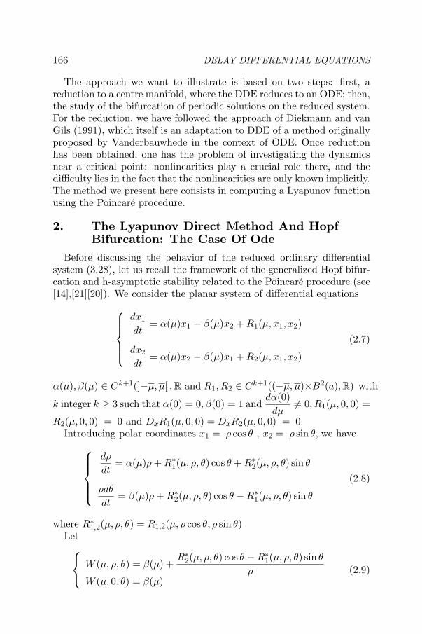
166 DELAY DIFFERENTIAL EQUATIONS
The approach we want to illustrate is based on two steps: first, areduction to a centre manifold, where the DDE reduces to an ODE; then,the study of the bifurcation of periodic solutions on the reduced system.For the reduction, we have followed the approach of Diekmann and vanGils (1991), which itself is an adaptation to DDE of a method originallyproposed by Vanderbauwhede in the context of ODE. Once reductionhas been obtained, one has the problem of investigating the dynamicsnear a critical point: nonlinearities play a crucial role there, and thedifficulty lies in the fact that the nonlinearities are only known implicitly.The method we present here consists in computing a Lyapunov functionusing the Poincare procedure.
2. The Lyapunov Direct Method And HopfBifurcation: The Case Of Ode
Before discussing the behavior of the reduced ordinary differentialsystem (3.28), let us recall the framework of the generalized Hopf bifur-cation and h-asymptotic stability related to the Poincare procedure (see[14],[21][20]). We consider the planar system of differential equations
dx1
dt= α(µ)x1 − β(µ)x2 + R1(µ, x1, x2)
dx2
dt= α(µ)x2 − β(µ)x1 + R2(µ, x1, x2)
(2.7)
α(µ), β(µ) ∈ Ck+1(]−µ, µ[ , R and R1, R2 ∈ Ck+1((−µ, µ)×B2(a), R) with
k integer k ≥ 3 such that α(0) = 0, β(0) = 1 anddα(0)dµ
= 0, R1(µ, 0, 0) =
R2(µ, 0, 0) = 0 and DxR1(µ, 0, 0) = DxR2(µ, 0, 0) = 0Introducing polar coordinates x1 = ρ cos θ , x2 = ρ sin θ, we have
dρ
dt= α(µ)ρ + R∗
1(µ, ρ, θ) cos θ + R∗2(µ, ρ, θ) sin θ
ρdθ
dt= β(µ)ρ + R∗
2(µ, ρ, θ) cos θ −R∗1(µ, ρ, θ) sin θ
(2.8)
where R∗1,2(µ, ρ, θ) = R1,2(µ, ρ cos θ, ρ sin θ)
Let
W (µ, ρ, θ) = β(µ) +R∗
2(µ, ρ, θ) cos θ −R∗1(µ, ρ, θ) sin θ
ρW (µ, 0, θ) = β(µ)
(2.9)

Introduction to Hopf Bifurcation theory DDE 167
For every ρ0 ∈ [0, a[ , θ0 ∈ R, the orbit of (2.7) passing through(ρ0, θ0) will be represented by the solution ρ(θ, µ0, θ0, ρ0) of the problem
dρ
dθ=
α(µ) + R∗1(µ, ρ, θ) cos θ −R∗
2(µ, ρ, θ) sin θ
W (µ, ρ, θ)= R(µ, ρ, θ)
ρ(µ, θ0) = ρ0
(2.10)When the function ρ(θ, µ0, θ0, ρ0) has been determined, complete in-formation of the solution of (2.7) will be obtained by integrating thefollowing equation
dθ
dt= W (µ, ρ(θ, µ0, θ0, ρ0), θ)
(µ, ρ, θ) ∈ ]−µ, µ[× [0, a[× [0, 2π]
(2.11)
Since α(0) = 0, it is easily seen by (2.9) and (2.10) that whena ∈ [0, a[ and µ are sufficiently small, then for any µ ∈ ]−µ, µ[ andc ∈ [0, a[ the solution of (2.11) exists in[0, 2π]. This solution will bedenoted by ρ(θ, µ, c)
Definition 29 [21]The function V(µ,c) = ρ(θ, µ, c) − c is called a dis-placement function of ( 2.7).For µ = 0, system ( 2.7) can be written in the form:
dx1
dt= −x2 + f1(x1, x2)
dx2
dt= x1 + f2(x1, x2)
(2.12)
where fi(x1, x2) = Ri(0, x1, x2) i = 1,2 (R1 and R2 are introduced informula ( 2.7).
Definition 30 [21] Let h be an integer, h ≥ 3. The solution x1 = x2
= 0 of ( 2.12) is said to be h-asymptotically stable (resp. h-completelyunstable) ifi) For every Θ, Σ ∈ C
(B2(a), R
)of order greater than h in (x1, x2), the
solution x1 = x2 = 0 of the system
dx1
dt= −x2 + f12(x1, x2) + ....f1h(x1, x2) + Θ(x1, x2)
dx2
dt= x1 + f22(x1, x2) + ....f2h(x1, x2) + Σ(x1, x2)
(2.13)

168 DELAY DIFFERENTIAL EQUATIONS
is asymptotically stable (resp.completely unstable)ii) Property i) not satisfied when h is replaced by any integer m ∈2, . . . , h− 1
Proposition 27 [21] Let h be an integer,h ≥ 3.The following asser-tions are equivalent:1) The solution x1 = x2 = 0 of ( 2.12) is h-asymptotically stable (resp.h-completely unstable).
3) There exists a Lyapunov function F such that the derivative of Falong the solution of ( 2.12) has the form:
•F (4.6) = Gh ‖ x ‖h+1 + o(‖ x ‖h+1)with Gh < 0 (resp. > 0), x = (x1, x2).
Remark 2 The Lyapunov function F is searched using the Poincareprocedure in the form
F (x) =h∑
j=1Fj(x),where the Fj
′s are homogeneous polynomials of
degree j in R2.
Theorem 3 [21](Generalized Hopf bifurcation theorem)Assume that the solution x1 = x2 = 0 of ( 2.12) is either 3-asymptoticallystable or 3-completely unstable. Then, there exists a real number µ > 0such that for µ ∈ ]−µ, µ[ , µnear 0, system ( 2.7) has exactly one peri-odic solution if α(µ)Gh < 0 and no periodic solution if α(µ)Gh > 0.
3. The Center Manifold Reduction Of DDELet us first very briefly draw the perspective of the center manifold
theorem. Consider a general nonlinear DDE
dx
dt= f(p, xt),
in which p represents a parameter (possibly, a vector). Assuming that
f(p, 0) = 0
for all p in a given region, the local behavior of the solutions near 0 isdependent upon the type of the linearized equation
dx
dt= Dϕf(p, 0)xt,
2) One has∂iV (0, 0)
∂ci= 0 for 1 ≤ i ≤ h − 1 and
∂hV (0, 0)∂ch
< 0
(resp.> 0), where V is the displacement function of ( 2.12), defined indefinition 29.

Introduction to Hopf Bifurcation theory DDE 169
which can itself be described in terms of the characteristic equation(providing the eigenvalues of the infinitesimal generator of the linearequation)
det(λI −Dϕf(p, 0)(exp(λ.)⊗ I)) = 0.
In the hyperbolic case, that is to say, as long as the equation has noroot with zero real part, solutions which remain close enough to theorigin either approach the origin at +∞ or escape from the origin. Inparticular, no periodic solution can be found in the vicinity of the originin this situation. This scenario, well known in the case of ODE, has beenextended to many infinitely dimensional cases, including DDE. It is aconsequence of the so-called saddle-point theorem which can be found,for example, in Hale’s books on DDE. We are concerned here with thenon hyperbolic case, that is, the situation that arises when for somep = π∗
c , the characteristic equation has a root with zero real part.Amongst the rich variety of cases, we choose one of the two simplestones: we assume that at p0, the characteristic equation has a pair ofimaginary roots, each simple, and no other multiple of these numbers(including 0) is a root of the equation.
To be more specific, we will consider the following example, the scalardelay differential equation
dx
dt= f(b, ε, xt), (3.14)
wheref(b, ε, ϕ) = −bϕ(−1) + ε(ϕ(−1))3 + o(ϕ3),
b and ε are two real parameters, b > 0, b >> |ε| . The vector of parame-ters is p = (b, ε). Equation (3.14) is an example of equations that hasbeen considered by many authors. An example of such an equation isthe logistic delay equation in the case of an odd nonlinearity
dx
dt= x(t)
1− x(t− 1)1 + x(t− 1)
(Change the variable from x to y = ln(x)).
3.1 The linear equation.The linear equation is
dx
dt= −bx(t− 1), (3.15)

170 DELAY DIFFERENTIAL EQUATIONS
There exists a scalar function η(θ) with bounded variation such that
−bϕ(−1) =∫ 0
−1[dη(θ)] ϕ(θ).
In fact, η(θ) may be chosen as
η(θ) =
0 if θ = −1−b if − 1 < θ ≤ 0.
The characteristic equation is obtained by substitution of
x(t) = eλtx0 (x0 ∈ C)
into the linear equation, that is
λ + be−λ = 0. (3.16)
Lemma 25 If we denote σ(A) (resp. Pσ(A)) the spectrum (resp. thepoint spectrum) of A, σ(A) = Pσ(A) and λ ∈ σ(A) if and only ifλ satisfies λ + be−λ = 0.
Lemma 26 All the roots of equation ( 3.16) have negative real part ifand only if 0 < b <
π
2.
Lemma 27 The characteristic equation ( 3.16) has two purely imagi-nary roots λ1,2 = ±i
π
2and all other roots have negative real parts if
b =π
2.
The adjoint equation: The formal dual product
< ψ,ϕ >= ψ(0)ϕ(0) +∫ 0
−1
∫ 0
θψ(s− θ)dη(θ)ϕ(s)ds
leads to
< ψ,ϕ >= ψ(0)ϕ(0)− b
∫ 0
−1ψ(s + 1)ϕ(s)ds (3.17)
for every pair ϕ ∈ Edef= C([−1, 0]; R), ψ ∈ E
∗ def= C([0, 1]; R).
The adjoint equation is:
dy(s)dt
=∫ 0
−1y(s− θ)dη(θ) = by(s + 1) (3.18)

Introduction to Hopf Bifurcation theory DDE 171
If y is a solution of (3.18) on an interval ]−∞, σ + 1[ then we let yt foreach t ∈ (−∞, σ) designate the element of E
∗ defined by
yt(s) = y(s + t) for 0 ≤ s ≤ 1.
We know that if x is a solution of (3.15) on τ − 1 < t < +∞ and y is asolution of (3.18) on (−∞, σ + 1) with σ > τ , then (yt, xt) is a constanton [τ, σ].
Let Λ =−i
π
2, +i
π
2
. Then ϕ1(θ) = sin
π
2θ, ϕ2(θ) = cos
π
2θ for−1 ≤
θ < 0 are two independent solutions of (3.15) in the case b =π
2. Simi-
larly, ψ∗1 (s) = sin
π
2s and ψ∗
2(s) = cosπ
2s are two independent solutions
of (3.18).Φ = (ϕ1, ϕ2) is a basis for the generalized eigenspace P = PΛ of (3.15)
and Ψ∗ = (ψ1, ψ2) is a basis for the generalized eigenspace P ∗Λ of (3.18)
associated with Λ. The bilinear form< ψj , ϕk > j, k = 1, 2 reads
< ψj , ϕk >= ψj(0)ϕk(0)− π
2
∫ 0
−1ψj(θ + 1)ϕk(θ)dθ; j, k = 1, 2 (3.19)
By defining a new basis, still denoted Ψ, for P ∗Λ we can make (Ψ, Φ) = I,
I is the identity matrix. We have: Ψ = col(ψ1,ψ2) where
ψ1(s) = 2µ0(sinπ
2s +
π
2cos
π
2s),
ψ2(s) = 2µ0(cosπ
2s +
π
2sin
π
2s).
with µ0 =1
1 +π2
2
. Denote Q = QΛ = ϕ :< ψj , ϕ >= 0, j = 1, 2 .
We have the decomposition E = P ⊕ Q. Hence any ϕ ∈ E can bewritten as ϕ = ϕP + ϕQ where ϕP = Φa0, a0 = col(a1, a2), that is,
a1 = µ0πϕ(0) + µ0π∫ 0−1(cos π
2 s− π2 sin π
2 s)ϕ(s)ds
a2 = 2µ0πϕ(0) + µ0π∫ 0−1(
π2 cos π
2 s + sin π2 s)ϕ(s)ds
(3.20)
If A is the infinitesimal generator of T (t), then we have A Φ = ΦB where
B =[
0 −π2
π2 0
].
Therefore T (t)Φ = ΦetB. Since ϕQ = ϕ − ϕP , ϕP = Φa0, a0 = (ψ, ϕ)it follows that ‖ T (t)ϕ−ΦeBta0 ‖ tends to 0 exponentially as t tends to

172 DELAY DIFFERENTIAL EQUATIONS
+∞, for every ϕ ∈ E. This means that any solution of (3.15) approachesa periodic function given by
a1 sinπ
2t + a2 cos
π
2t
where a1 and a2 are given by (3.20).
3.2 The center manifold theoremHere, we go through the derivation of the centre manifold made by
Diekmann and van Gils. There is part of the method which is generaland follows in fact the approach by Vanderbauwhede, and part whichis implicated by the delay: essentially, the treatment of the variation ofconstant formula using the sun-star extension. I will first state the basicproblem, taking a general equation:
dx
dt= Lxt + F (xt) (3.21)
We assume that F is smooth, F (0) = 0, DF (0) = 0. Moreover, I assumethat the linear part L has only a stable and a center part, which leadsto a decomposition of the state space
E = EC ⊕ ES
which corresponds toI = πC + πS .
Using the variation of constants formula, equation (3.21) reads as
xt = T (t)ϕ +∫ t
0T∗(t− s)F (xs)ds
which decomposes onto the subspaces Ec and Es as follows
πC(xt) = TC(t)ϕC +∫ t
0πCT∗(t− s)F (xs)ds
πS(xt) = TS(t)ϕS +∫ t
0πST∗(t− s)F (xs)ds.
Looking for solutions defined on the whole real axis and uniformly boundedon their domain, the second identity can be written starting from anyinitial point σ
πS(xt) = TS(t− σ) (xσ)S +∫ t
σπST∗(t− s)F (xs)ds.

Introduction to Hopf Bifurcation theory DDE 173
Letting σ → −∞, the term TS(t − σ) (xσ)S approaches 0, while theintegral has a limit, which yields an expression where the projection ϕS
has been eliminated
πS(xt) =∫ t
−∞πST∗(t− s)F (xs)ds.
This leads to the following expression for xt
xt = TC(t)ϕC +∫ t
0πCT∗(t− s)F (xs)ds +
∫ t
−∞πST∗(t− s)F (xs)ds.
(3.22)In fact, the above formulas are not correct, the projector πC is definedon E, thus it is necessary to extend it to the space EC in order to use it inthe above expressions. The fact that it can be done in some natural wayis proved in the paper by Diekmann and van Gils, who use the followingformula, (with the notation π∗
C used for the extension)
π∗C =
12πi
∫Γ(zI −A∗)−1dz
(Γ is a contour enclosing the imaginary roots and no other root)The following expression is established
π∗C (β, h) =
12πi
∫Γ
ezθ(zI − Lz)−1
[β + L
∫ 0
ηez(η−s)h(s)ds
]dz,
(3.23)with the same meaning for Γ, Lz = L (ez.) and (β, h) ∈ E
∗ ∼= Rn ×
L∞ ([−1, 0] , Rn). In terms of π∗C , (3.22) reads
xt = TC(t)ϕC +∫ t
0
π∗C T∗(t− s)F (xs)ds+
∫ t
−∞
(I − π∗
C
)T∗(t− s)F (xs)ds
(3.24)Note that π∗
C is still a projection onto a finite dimensional subspace, infact, it has the same range as πC . In order to set up the full equation forthe center manifold, there are still two steps: 1) localizing the equationusing a truncation; 2) choosing a suitable state space in which the fixedpoint problem defined by (3.24) makes sense.
Proposition 28 π∗C is an extension of πC to the space and we have
π∗C Φ =< ψ1, Φ > ϕ1+ < ψ2, Φ > ϕ2 for any Φ = (β, h) ∈ E
∗
ψj and ϕj (j = 1, 2) are respectively the basis of the space E∗c and Ec.

174 DELAY DIFFERENTIAL EQUATIONS
Proof. We first consider the case when h = 0. Then, formula (3.23)reduces to
π∗c (β, 0) =
12πi
∫Γ
(ezθ(zI − Lz)−1β
)dz =
12πi
∫Γ
ezθ ∆ (z)p (z)
βdz,
where ∆ (z) is the cofactor matrix of the matrix zI − Lz and p(z) =det(zI − Lz). Using the residue theorem, we obtain
π∗c (β, 0) =
(ei π
2 ∆(iπ2 )
p′(iπ2 )
+e−i π
2 ∆(−iπ2 )
p′(−iπ2 )
)β.
In the case we are considering here, ±iπ
2are of multiplicity 1 and the
basis functions ϕj and ψj j = 1, 2 of Ec and E∗c may be written in the
form ϕj = eiθvj and ψj = eiθwj , j = 1, 2 , with(iπ
2I − Li π
2
)vj = 0 and wj
(iπ
2I − Li π
2
)= 0.
Since iπ
2is of multiplicity 1, we have
R(∆(iπ
2
))= v1
andR(∆ (iπ
2
))=
w 1
which implies w1v1 = 0. R(∆(iπ
2
))and R
(∆ (iπ
2
))denotes the
range of the linear operators ∆(iπ
2
)and ∆
(iπ
2
), respectively.
Then, we deduce that ∆(iπ
2
)= v1w1. So,
π∗c (β, 0) =
(ei π
2 v1w1
p′(iπ2 )
+e−i π
2 v2w2
p′(−iπ2 )
)β.
Hence,
π∗c (β, 0) = (w1, β)ϕ1 + (w2, β)ϕ2, with wj = ψj(0). (3.24)
Let ϕ ∈ E = C([−1, 0], R) be such that ϕ(0) = 0. Formula (3.23) yields
π∗c (0, ϕ) =
12πi
∫Γ
[ezθ(zI − Lz)−1L
ezθ
∫ 0
θezsϕ(s)ds
]dz.

Introduction to Hopf Bifurcation theory DDE 175
We may observe that the right hand side of the above formula is equalto P0ϕ, which, on the other hand, can be represented in terms of theformal dual product using formula (3.23). Therefore, we have
π∗c (0, ϕ) = (ψ1, ϕ)ϕ1 + (ψ2, ϕ)ϕ2, such that ϕ(0) = 0.
Since the space IE0 = ϕ ∈ E, ϕ(0) = 0 is dense in L1([−1, 0], R), theabove formula holds for any (0, ϕ) ∈ E
∗. Combining the above tworesults, we deduce that for any (β, h) ∈ E
∗ we have :
π∗c (β, h) = (ψ1, (β, h))ϕ1 + (ψ2, (β, h))ϕ2,
where <, > is the extension of the formal dual product given by formula(3.17).The proof of Proposition 33 is complete.
The spectrum σ(A) is a pure point spectrum. Ec is a two dimensionalspace on which T∗(t) can be extended to a group on R. Moreover thedecomposition is an exponential dichotomy on R, that is for any β > 0,there exists a positive constant k = k(β) such that
‖T (s)x‖ ≤ k exp(β |s|) ‖x‖ , for s ≥ 0 and x ∈ E0,∥∥T (s)x∗∥∥ ≤ k exp((γ + β) |s|)∥∥x∗∥∥ , for s ≥ 0 and x∗ ∈ E
∗s ,
whereγ = sup
Reλ, λ ∈ Pσ(A∗) and Reλ < 0
.
Observe that we have the same properties for the space R2×E
∗, that isR
2×E∗ =
(R
2 ×Ec
)⊗E
∗s and
(R
2 × Ec
)is a finite dimensional space
invariant by T ∗(t) T (t). For a moment, let us consider the generalnon homogeneous equation associated with (3.35), that is:
v(t) = T (t− s)v(s) +∫ t
sT ∗(t− s)h(s)ds. (3.25)
The Center manifold theorem. Let us recall a few definitions
Definition 31 [33]BCν(R, IE) is the space of all continuous function ffrom R into E such that
supR
(exp (−νt)) ‖f(t)‖ <∞.
For ν = 0,we write BC(R, E). BCν(R, E) is a Banach space when en-dowed with the norm
‖f‖ν = supR
(exp (−νt)) ‖f(t)‖ <∞.
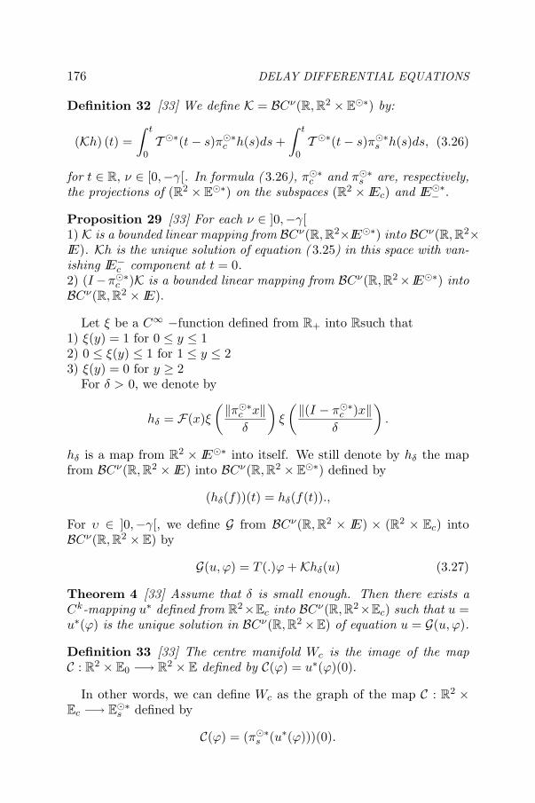
176 DELAY DIFFERENTIAL EQUATIONS
Definition 32 [33] We define K = BCν(R, R2 × E∗) by:
(Kh) (t) =∫ t
0T ∗(t− s)π∗
c h(s)ds +∫ t
0T ∗(t− s)π∗
s h(s)ds, (3.26)
for t ∈ R, ν ∈ [0,−γ[. In formula ( 3.26), π∗c and π∗
s are, respectively,the projections of (R2 × E
∗) on the subspaces (R2 × IEc) and IE∗− .
Proposition 29 [33] For each ν ∈ ]0,−γ[1) K is a bounded linear mapping from BCν(R, R2×IE∗) into BCν(R, R2×IE). Kh is the unique solution of equation ( 3.25) in this space with van-ishing IE−
c component at t = 0.2) (I−π∗
c )K is a bounded linear mapping from BCν(R, R2× IE∗) intoBCν(R, R2 × IE).
Let ξ be a C∞ −function defined from R+ into Rsuch that1) ξ(y) = 1 for 0 ≤ y ≤ 12) 0 ≤ ξ(y) ≤ 1 for 1 ≤ y ≤ 23) ξ(y) = 0 for y ≥ 2
For δ > 0, we denote by
hδ = F(x)ξ(‖π∗
c x‖δ
)ξ
(‖(I − π∗
c )x‖δ
).
hδ is a map from R2 × IE∗ into itself. We still denote by hδ the map
from BCν(R, R2 × IE) into BCν(R, R2 × E∗) defined by
(hδ(f))(t) = hδ(f(t)).,
For υ ∈ ]0,−γ[, we define G from BCν(R, R2 × IE) × (R2 × Ec) intoBCν(R, R2 × E) by
G(u, ϕ) = T (.)ϕ +Khδ(u) (3.27)
Theorem 4 [33] Assume that δ is small enough. Then there exists aCk-mapping u∗ defined from R
2×Ec into BCν(R, R2×Ec) such that u =u∗(ϕ) is the unique solution in BCν(R, R2×E) of equation u = G(u, ϕ).
Definition 33 [33] The centre manifold Wc is the image of the mapC : R
2 × E0 −→ R2 × E defined by C(ϕ) = u∗(ϕ)(0).
In other words, we can define Wc as the graph of the map C : R2 ×
Ec −→ E∗s defined by
C(ϕ) = (π∗s (u∗(ϕ)))(0).

Introduction to Hopf Bifurcation theory DDE 177
Now lety(t) = (π∗
c (u∗(ϕ)))(0)(t).
Then y satisfies the equation:
y(t) = T (t)y(0) +∫ t
0T ∗(t− s)π∗
c hδ(C(y(s)))ds. (3.28)
Differentiating (3.28), we obtain
dy
dt= Ay(t) + π∗
c hδ(C(y(t))), y(t) ∈ R2 × Ec. (3.29)
We writey(t) = (b, ε, z(t)) ∈ R
2 × Ec
where z(t) ∈ Ec. Therefore
C(y(t)) ∈ R2 × Ec ⊕ E
∗s
Then we can write:
C(y(t)) = (b, ε, z(t),M(b, ε, z(t))) where M(b, ε, z(t)) ∈ R2 × E
∗s .
3.3 Back to the nonlinear equation:Now, consider the nonlinear delay equation:
dx(t)dt
= −bx(t− 1) + εx3(t− 1) + o((xt)
3)
. (3.30)
(3.30) may be written in the form:
dx(t)dt
=∫ 0
−1dη(s)x(t− s) + g(ε, xt), (3.31)
g(ε, ϕ) = εϕ3(−1) + o((ϕ)3
)with the initial condition: x(θ) = ϕ(θ) for
−1 ≤ θ ≤ 0; ϕ ∈ X = E.Returning to the nonlinear delay equation (3.30) , we supplement
it with two trivial equationsdb
dt= 0 and
dε
dt= 0. Precisely, we are
concerned in the sequel with the system of delay equations
dx
dt= Lxt + N(b, ε, xt),
db
dt= 0,
dε
dt= 0,
(3.32)

178 DELAY DIFFERENTIAL EQUATIONS
withN(b, ε, xt) = −(b− π
2)x(t− 1) + g(ε, xt)
andLxt = −π
2x(t− 1).
Equation (3.32) may be interpreted as an evolution equation of theform:
where A is the infinitesimal generator of the semi-group T (t), solution
of the linear equationdx
dt= Lxt and r∗ = (I, 0).
We note that the map
ϕ −→ r∗N(b, ε, xt)
is defined from E into E∗. If we identify ϕ ∈ E with (ϕ(0), ϕ) ∈ E
then equation (3.33) may be written in the form:
F is a continuous function defined from R3 × E into E
∗ and u = xt .The variation of constant formula in this case is
v(t) = T (t− s)v(s) +∫ t
sT ∗(t− s)F(v(s))ds (3.35)
withv(t) = (b, ε, u(t)),F(v(t)) = (F (b, ε, u(t)), 0, 0)
andT (b, ε, u(t)) = (b, ε, T (t)ϕ).
Hence, the ordinary equation (3.29) becomes, in our case,
d
dt(xt) = Axt + r∗N(b, ε, xt),
db
dt= 0,
dε
dt= 0,
(3.33)
du
dt=
(A∗
0 + r∗L)u + F (b, ε, xt),
db
dt= 0,
dε
dt= 0.
(3.34)
dz(t)
dt=
Bz(t) + β (Φz (t) + M(b, ε, z(t)) (−1)) + ε (Φz (t) +M(b, ε, z(t)) (−1))3 +
o (Φz (t) + M(b, ε, z(t)) (−1))3 ψ(0)dβ
dt= 0
dε
dt= 0
(3.36)

Introduction to Hopf Bifurcation theory DDE 179
with
ψ(0) =(
µ0π2µ0
), µ2 =
1
1 +π2
2
, Φ =(−1
0
)and β = b− π
2.
So we obtain:
Note that M(b, ε, 0) = 0,d
dtM(b, ε, 0)z = z and z −→ M(b, ε, z) is
Ck with k ≥ 2, since g is a C∞ function with respect to ϕ, satisfyingg(ε, 0) = 0, Dg(ε, 0) = 0. From now on, we will be concerned with theordinary differential equation in R
2 parametrized by β and ε (β and εare in the neighborhood of 0). The next section will be devoted to theexistence of periodic solutions of the equation
3.4 The reduced systemWe are now in a position to discuss the behavior of the reduced ordi-
nary differential system.We first concentrate on the case β = 0 ( β is defined in section 3,
β = 0 corresponds to b = π2 ). In this case, our ODE is reduced to
ddt
z1(t) = −π2
z2(t) + εµ0π [−z1(t) + M(ε, z(t))(−1)]3 + o [−z1(t) + M(ε, z(t))(−1)]3
ddt
z2(t) = π2
z1(t) + 2εµ0 [−z1(t) + M(ε, z(t))(−1)]3 + o [−z1(t) + M(ε, z(t))(−1)]3
(3.39)where M(ε, z(t)(−1)) = M(0, ε, z(t)(−1)).
Since M(β, ε, 0) = 0 and∂M(β, ε, 0)
∂zz = z, M(β, ε, z(t))(−1) is a
o(‖ z ‖) that isM(β, ε, z)‖ z ‖ → 0 as z → 0.
d
dtz1(t) =
−π
2z2(t) + M(b, ε, z(t)) (−1) + εµ0π (−z1 (t) + M(b, ε, z(t)))3 +
o (−z1 (t) + M(b, ε, z(t)))3
d
dtz2(t) =
(π2 + µ0πβ)z1(t) − 2βµ0M(b, ε, z(t)) (−1) +
2µ0ε (−z (t) + M(b, ε, z(t)) (−1))3 + o (−z1 (t) + M(b, ε, z(t)))3
dβ
dt= 0
dε
dt= 0
(3.37)
d
dtz1(t) =
−π2 z2(t) + M(b, ε, z(t)) (−1) + εµ0π (−z1 (t) + M(b, ε, z(t)))3
+o (−z1 (t) + M(b, ε, z(t)))3
ddtz2(t) =
(π2 + µ0πβ)z1(t) − 2βµ0M(b, ε, z(t)) (−1) +
2µ0ε (−z (t) + M(b, ε, z(t)) (−1))3 + o (−z1 (t) + M(b, ε, z(t)))3
(3.38)

180 DELAY DIFFERENTIAL EQUATIONS
A natural candidate to be the principal part of system (3.39) is thesystem
Proposition 30 The origin z = 0 of ( 3.40) is 3-asymptotically stableif ε > 0 (3-completely-unstable if ε < 0).
Before we proceed to the proof of proposition 4.2, let us derive itsconsequences on equation (3.14).
Corollary 5 The origin of equation ( 3.14).is asymptotically stable ifε > 0 and unstable if ε < 0.
Proof of Corollary 5Equation (3.39) is a perturbation of order o(‖ z ‖3) of equation (3.40).
Therefore, it enjoys the same stability properties as equation (3.40),when the latter is either 3-asymptotically stable or 3-completely unsta-ble. Since equation (3.39) is the reduced equation of equation (3.14) onthe centre manifold we deduce from the fundamental centre manifoldtheorem that the two equations have the same stability properties, thatis the origin of (3.14).is asymptotically stable if ε > 0 and unstable ifε < 0.Proof of Proposition 4.2Proving that the origin of (3.40) is 3-asymptotically stable (resp. 3-completely-unstable) is equivalent to determining a Lyapunov functionF of the form
F (z1, z2) = z21 + z2
2 + F3 (z1, z2) + F4(z1, z2)
such that•F (z1, z2) = Gh( z2
1 + z22)
2 + o(‖ (z1, z2) ‖4
)(3.41)
with Gh < 0 (resp. Gh > 0 ), ( F3 and F4 are two homogeneouspolynomials of degree 3 and 4 respectively).
We have•F (z1, z2) =
(−π
2z2
) ∂F
∂z1+(π
2z2
) ∂F
∂z2−(εµ0πz3
1
) ∂F
∂z1−(2εµ0z
31
) ∂F
∂z2,
that is•F (z1, z2) =
(−π
2z2
)∂F3∂z1
+(
π2z2
)∂F3∂z2
−(εµ0πz3
1
)∂F3∂z1
−(2εµ0z
31
)∂F4∂z2
+(−π
2z2
)∂F4∂z1
+(
π2z2
)∂F4∂z2
−(εµ0πz3
1
)∂F4∂z1
−(2εµ0z
31
)∂F4∂z2
− 2εµ0πz41 − 4εµ0z
31z2.
ddtz1(t) = −π
2 z2(t) − εµ0π [z1(t) ]3ddtz2(t) = π
2 z1(t) − 2εµ0 [−z1(t) ]3(3.40)

Introduction to Hopf Bifurcation theory DDE 181
Let T denote the operator −z∂
∂z1+ z1
∂
∂z2and Tj its restriction to
the space Pj of homogeneous polynomials of degree j. We know from[14] that Tj is a bijection from Pj to Pj when j is odd. Then, equatingterms with the same degree on both sides of (3.41), we arrive at
π
2T3F3 = 0, that is F3 = 0,
π
2T4F4 = G4
(z21 + z2
2
)2 + 2µ0επz41 + 4µ0εz
31z2 (3.42)
and−(εµ0z
31
) ∂F4
∂z1−(2εµ0z
31
) ∂F4
∂z2= o((
z21 + z2
2
)2).
F4 is a homogeneous polynomial of degree 4,
F4 = a1z41 + a2z
31z2 + a3z
21z
22 + a4z1z
32 + a5z
42 , (ai ∈ R, for 1 ≤ i ≤ 5).
Formula (3.42) yields a system of linear equations,
a2 = 2πG4 + 4εµ0
a3 − 2a1 = 4πµ0ε
a4 − a2 = 43πG4
2a5 − a3 = 0−a4 = 2
πG4
from which we deduce
G4 (ε) = −34µ0επ, (3.43)
a4 =32µ0ε, a2 =
52µ0ε, a5
12a3, a1 =
12a3 −
2π
µ0ε; a3 ∈ R.
We know from [14] that the homogenous polynomials of even degree j aredetermined up to the addition of constant terms
(z21 + z2
2
)j . Therefore,we can choose a3 = 0 and the Lyapunov function F is
F (z1, z2) = z21 + z2
2 −2π
µ0εz41 +
52µ0εz
31z2 +
32µ0εz1z
32 .
We observe that G4 (ε) < 0 if ε > 0 and G4 (ε) > 0 if ε < 0. This meansthat system (3.40) is 3-asymptotically stable if ε > 0 and 3-completelyunstable if ε < 0.
Proposition 31 Suppose f (b, ε, ϕ) = −bϕ(−1)+ε (ϕ(−1))3+a (ϕ (−1))5.For ε = 0, β = 0 and a = 0, the origin x = 0 is 5-asymptotically stable(respectively, 3-completely unstable) if a > 0 (resp. a < 0).

182 DELAY DIFFERENTIAL EQUATIONS
Proof. The reduced ordinary differential system associated to (3.14)becomes
The candidate to be the principal part of (3.44) is the system:
Using once again the Poincare procedure, we show that the functiongiven by
F (z1, z2) = z21 + z2
2 −43π
aµ0z61 −
114
aµ0z51z2 +
103
µ0az31z
32 +
54aµ0πz1z
52
is a Lyapounov function of system (3.45). Its derivative along the solu-tions of (3.45) is
.F (z1, z2) = −5
4aµ0π
(z21 + z2
2
)3 + o((
z21 + z2
2
)3).
Thus, near the origin,.F has the sign of −a, which gives the conclusion
of the propositionRemark 4.2System (3.39) is a perturbation of system (3.40). From Proposition30 and generalized Hopf bifurcation theorem, Theorem 3, we can onlyconcude that system (3.39) has no more than one periodic solution.Because the linear part of this system is independant of the parameterε, the condition given in terms of the sign of α (µ) Gh (see Theorem 3)is not fulfiled.
4. Cases Where The Approximation Of CenterManifold Is Needed
Let f be a real function defined on IR. Reconsider the delay equation
x′ (t) = f (x (t− 1)) . (4.46)
Assume that f satisfies the following assumptions
(H) :
f ∈ Ck (IR) for some k ≥ 3f (0) = 0.
ddtz1(t) = −π
2 z2(t) + εµ0π [−z1(t) + M(β, ε, z(t))(−1)]3
+aµ0π [−z1(t) + M(β, ε, z(t))(−1)]5ddtz2(t) = π
2 z1(t) + 2εµ0 [−z1(t) + M(β, ε, z(t))(−1)]3
+2aµ0 [−z1(t) + M(β, ε, z(t))(−1)]5(3.44)
ddtz1(t) = −π
2 z2(t) − aµ0πz51(t)
ddtz2(t) = π
2 z1(t) − 2aµ0z51(t)
(3.45)

Introduction to Hopf Bifurcation theory DDE 183
Equation (4.46) may be written as
x′ (t) = −γx (t− 1) + αx2 (t− 1) + εx3 (t− 1) + o(x3 (t− 1)
), (4.47)
where γ = −f ′ (0) , α = 12f ′′ (0) and ε = 1
3!f′′′ (0) .
In the last section, f ′′(0) = 0.If we use the method developed before. The presence of a quadratic
term in equation (4.47) creates an additional difficulty compared to thesituation dealt with in the last section, also in several other works whereit is assumed that the nonlinearity is odd. The determination of theLyapunov function leads us to give an explicit approximation of thehomogeneous part of degree two of the local center manifold near zeroassociated to equation (4.47) for the value γ =
π
2.
It is also possible to extend the procedure to compute a center mani-fold for a general autonomous functional differential equation.
4.1 Approximation of a local center manifoldLet us now briefly describe what the local center manifold theorem
tells us. For the most recent and satisfactory presentation of this result,we refer to Diekmann and van Gils [33]. So, equation (4.47) has a localcenter manifold
M : U × V −→ Xs
(β, ξ) −→ M (β, ξ) ,
where U (resp. V ) is a neighborhood of zero in IR ( resp. IR2).On this center manifold the delay equation (4.47) is reduced to an
ordinary differential one, given by
dz (t)dt
= Bz (t) + Ψ (0) [−β (Φ (−1) z (t) + M (β, z (t)) (−1))
+α (Φ (−1) z (t) + M (β, z (t)) (−1))2
+ε (Φ (−1) z (t) + M (β, z (t)) (−1))3
+o((Φ (−1) z (t) + M (β, z (t)) (−1))3
)]
dβ (t)dt
= 0,
(4.48)
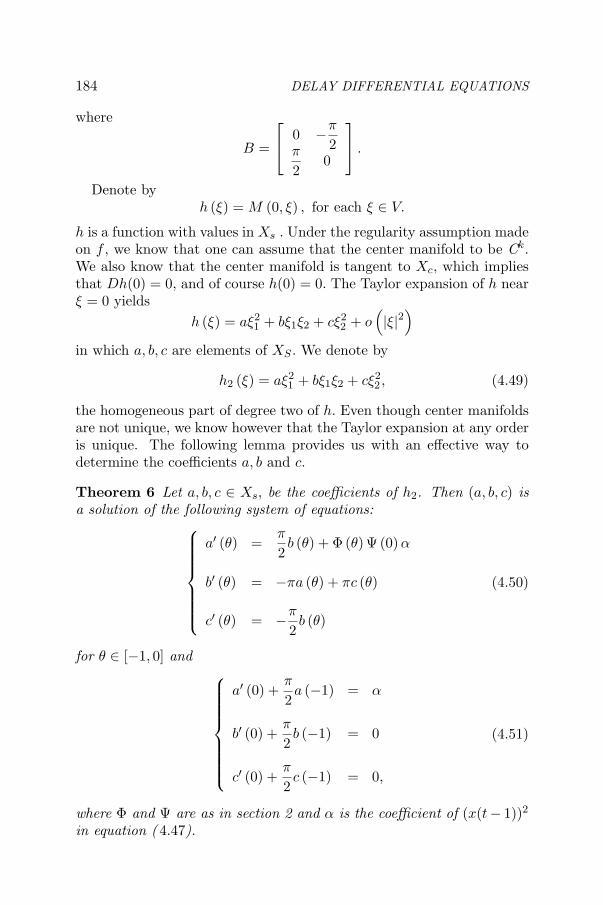
184 DELAY DIFFERENTIAL EQUATIONS
where
B =
0 −π
2π
20
.
Denote byh (ξ) = M (0, ξ) , for each ξ ∈ V.
h is a function with values in Xs . Under the regularity assumption madeon f , we know that one can assume that the center manifold to be Ck.We also know that the center manifold is tangent to Xc, which impliesthat Dh(0) = 0, and of course h(0) = 0. The Taylor expansion of h nearξ = 0 yields
h (ξ) = aξ21 + bξ1ξ2 + cξ2
2 + o(|ξ|2)
in which a, b, c are elements of XS . We denote by
h2 (ξ) = aξ21 + bξ1ξ2 + cξ2
2 , (4.49)
the homogeneous part of degree two of h. Even though center manifoldsare not unique, we know however that the Taylor expansion at any orderis unique. The following lemma provides us with an effective way todetermine the coefficients a, b and c.
Theorem 6 Let a, b, c ∈ Xs, be the coefficients of h2. Then (a, b, c) isa solution of the following system of equations:
a′ (θ) =π
2b (θ) + Φ (θ) Ψ (0) α
b′ (θ) = −πa (θ) + πc (θ)
c′ (θ) = −π
2b (θ)
(4.50)
for θ ∈ [−1, 0] and
a′ (0) +π
2a (−1) = α
b′ (0) +π
2b (−1) = 0
c′ (0) +π
2c (−1) = 0,
(4.51)
where Φ and Ψ are as in section 2 and α is the coefficient of (x(t− 1))2
in equation ( 4.47).

Introduction to Hopf Bifurcation theory DDE 185
Proof : For every ξ ∈ V , denote by z (t) the solution of the ordinarydifferential equation
dz (t)dt
= Bz (t) + Ψ (0) g (Φ (−1) z (t) + h (z (t)) (−1))
z (0) = ξ,
(4.52)
where g (x) =π
2x + f (x) =
π
2x +
(−γx + αx2 + εx3 + o
(x3))
.
The first property of a center manifold is that it is invariant with respectto the original semiflow. So, if z is a solution of equation (3.19), then,the function t −→ Φz (t)+h (z (t)) is a solution of equation (4.47). This,in particular, implies that it verifies the translation property, for eacht ∈ [0, 1] and θ ∈ [−1,−t] (ie : t + θ ≤ 0),
Φ (θ) z (t) + h (z (t)) (θ) = Φ (t + θ) ξ + h (ξ) (t + θ) . (4.53)
By differentiating equation (4.53) with respect to t and rearrangingterms,
∂h (ξ)
∂θ(t + θ) + Φ (t + θ) Bξ =
[Φ (θ) +
∂h
∂z(z (t)) (θ)
]
× [Bz (t) + Ψ (0) g (Φ (−1) z (t) + h (z (t)) (−1))] .
(4.54)
So, letting t go to 0, from above , it follows that
∂h (ξ)∂θ
(θ) =∂h
∂z(ξ) (θ) [Bξ + Ψ (0) g (Φ (−1) ξ + h (ξ) (−1))]
+ Φ (θ) Ψ (0) g (Φ (−1) ξ + h (ξ) (−1)) .(4.55)
On the other hand, the local semi flow t −→ Φz (t) + h (z (t)) generatedby the delay equation (4.47) with γ =
π
2on the center manifold is
differentiable at t = 0. So,∂
∂θ[Φξ + h (ξ)] (0) = −π
2[Φ (−1) ξ + h (ξ) (−1)]+g (Φ (−1) ξ + h (ξ) (−1)) ,
which implies
∂h (ξ)∂θ
(0) = −π
2h (ξ) (−1) + g (Φ (−1) ξ + h (ξ) (−1)) . (4.56)
The homogeneous part of degree two with respect to ξ of (4.55) and(4.56)respectively, is given by
∂h2 (ξ)∂θ
(θ) =∂h2
∂z(ξ) (θ) [Bξ] + Φ (θ) Ψ (0) g2 (Φ (−1) ξ) (4.57)

186 DELAY DIFFERENTIAL EQUATIONS
and∂h2 (ξ)
∂θ(0) = −π
2h2 (ξ) (−1) + g2 (Φ (−1) ξ) . (4.58)
Then, if we note that g2 (x) = αx2, conditions (4.50) and (4.51) followrespectively from (4.57) and (4.58).
Remark We already know that (a, b, c) are unique as coefficients ofthe quadratic part of the Taylor expansion of h. However, it is not ob-vious from the beginning that the system of equations (4.50) and (4.51)they satisfy determines these coefficients in a unique way. The followingproposition provides us with uniqueness of the solution of that systemof equations.
Proposition 32 The solution of the ordinary differential equation ( 4.50)with the boundary conditions ( 4.51) is unique.
Proof : Put
H =
0π
20
−π 0 π
0π
20
and X =
a
bc
.
By the use of the variation of constant formula, the general solution of(4.50) is given by
X (θ) = exp (Hθ) X (0) + S (θ) ,
where
S (θ) =∫ θ
0exp (H (θ − s)) col (Φ (s) Ψ (0)α , 0 , 0) ds.
The boundary condition (4.51) reads[H +
π
2exp (−H)
]X (0)+col (Φ (s) Ψ (0) α , 0 , 0)+
π
2S (−1) = col (α, 0, 0) .
(4.59)Hence, if we notice that
exp (Hθ) =
12 [1 + cos (πθ)] 1
2 sin (πθ) 12 [1− cos (πθ)]
− sin (πθ) cos (πθ) sin (πθ)
12 [1− cos (πθ)] −1
2 sin (πθ) 12 [1 + cos (πθ)]
, (4.60)
then, by virtue of (4.59), it follows that X (0) is a solution of the linearsystem
DX (0) = e, (4.61)

Introduction to Hopf Bifurcation theory DDE 187
where
D =
0 1 1−2 −1 21 −1 0
and
e = −S (−1) + col
(2α
π(1− 2µ0) , 0 , 0
).
Since the matrix D is invertible, hence, existence and uniqueness ofX (0) are ensured from (4.61) . Therefore, existence and uniqueness ofthe solution of (4.50) and (4.51) hold.
Corollary 7 Let a, b, c ∈ C. (a, b, c) are the coefficients of the quadraticpart of the Taylor expansion of h if and only if (a, b, c) is the solution ofthe system of equations (4.50) and (4.51) .
Corollary 8 If a, b, c ∈ Xs are the coefficients of h2, then
a (−1) =6α
5π− 4αµ0
3π
b (−1) = −4α
5π+
4αµ0
3
c (−1) =4α
5π− 8αµ0
3π.
Proof : By virtue of the expression (4.60) of exp (Aθ), it follows that
S (−1) = col
(4µ0α
3− 4µ0α
3π,
4µ0α
3− 8µ0α
3π,
2µ0α
3− 8µ0α
3π
)
Moreover, the inverse matrix of D is given by
D−1 =15
2 −1 3
2 −1 −23 1 2
.
Hence, from (4.61) it follows that
X (0) = col
(4α
5π− 2αµ0
3,
4α
5π− 8αµ0
3π,
6α
5π− 4αµ0
3
).
So, by substituting the expressions of a (0) , b (0) and c (0) in the equation(4.51) , the result follows immediately .
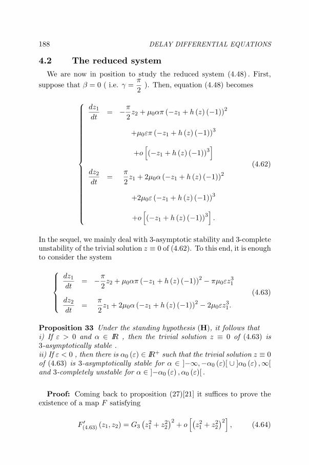
188 DELAY DIFFERENTIAL EQUATIONS
4.2 The reduced systemWe are now in position to study the reduced system (4.48) . First,
suppose that β = 0 ( i.e. γ =π
2). Then, equation (4.48) becomes
dz1
dt= −π
2z2 + µ0απ (−z1 + h (z) (−1))2
+µ0επ (−z1 + h (z) (−1))3
+o[(−z1 + h (z) (−1))3
]
dz2
dt=
π
2z1 + 2µ0α (−z1 + h (z) (−1))2
+2µ0ε (−z1 + h (z) (−1))3
+o[(−z1 + h (z) (−1))3
].
(4.62)
In the sequel, we mainly deal with 3-asymptotic stability and 3-completeunstability of the trivial solution z ≡ 0 of (4.62). To this end, it is enoughto consider the system
dz1
dt= −π
2z2 + µ0απ (−z1 + h (z) (−1))2 − πµ0εz
31
dz2
dt=
π
2z1 + 2µ0α (−z1 + h (z) (−1))2 − 2µ0εz
31 .
(4.63)
Proposition 33 Under the standing hypothesis (H), it follows thati) If ε > 0 and α ∈ IR , then the trivial solution z ≡ 0 of (4.63) is3-asymptotically stable .ii) If ε < 0 , then there is α0 (ε) ∈ IR+ such that the trivial solution z ≡ 0of (4.63) is 3-asymptotically stable for α ∈ ]−∞,−α0 (ε)[ ∪ ]α0 (ε) ,∞[and 3-completely unstable for α ∈ ]−α0 (ε) , α0 (ε)[ .
Proof: Coming back to proposition (27)[21] it suffices to prove theexistence of a map F satisfying
F ′(4.63) (z1, z2) = G3
(z21 + z2
2
)2 + o[(
z21 + z2
2
)2], (4.64)

Introduction to Hopf Bifurcation theory DDE 189
with G3 ∈ IR \ 0 . In [14], the authors have proved that such a mapmay be computed using the Poincare procedure,
F (z) =4∑
j=1
Fj (z) , (4.65)
where Fj is a homogeneous polynomial of degree j.Let F be a functional having the form (4.65). Then
F ′(4.63) (z1, z2) =
π
2T2F2 +
π
2T3F3 +
π
2T4F4
+
(∂F2
∂z1+
∂F3
∂z1+
∂F4
∂z1
)(µ0απ (−z1 + h (z) (−1))2 − πµ0εz3
1
)
+
(∂F2
∂z2+
∂F3
∂z2+
∂F4
∂z2
)(2µ0α (−z1 + h (z) (−1))2 − 2µ0εz3
1
),
where Tj is a linear operator defined on the space of homogeneous poly-nomials of degree j by
TjP = −z2∂P
∂z1+ z1
∂P
∂z2.
The expression of F ′(4.63) (z1, z2) is desired to be of the form (4.64) , which
is equivalent to the three relations :(i) T2F2 = 0.
(ii)π
2T3F3 +
(π
∂F2
∂z1+ 2
∂F2
∂z2
)(µ0αz2
1
)= 0.
(iii)
G3z41 + 2G3z2
1z22 + G3z4
2 =π
2T4F4 +
(π
∂F3
∂z1+ 2
∂F3
∂z2
)(µ0αz2
1
)
+
(π
∂F2
∂z1+ 2
∂F2
∂z2
)(−2µ0αP (z) z1 − µ0εz3
1
),
where P (z) = h2 (z) (−1) . For notational convenience, we denote bym1, m2 and m3 respectively a (−1) , b (−1) and c (−1) , where a, b, c ∈ Xs
denote the coefficients of h2 (z). Now, we shall exploit relations (i),(ii)and (iii) to derive a Lyapunov function F :Relation (i) implies that
F2 (z) = r(z21 + z2
2
), for r ∈ IR.
Without loss of generality, we put r = 1. Relation (ii) implies that
F3 (z) = 4µ0α
[23π
z31 − z2
1z2 −23z32
].

190 DELAY DIFFERENTIAL EQUATIONS
Finally, if we define
F4 (z) = a1z41 + a2z
31z2 + a3z
21z
22 + a4z1z
32 + a5z
42 ,
then, the relation (iii) is equivalent to
π
2a2 − 2π (2µ0αm1 + εµ0) = G3
π
2(2a3 − 4a1)− 4µ0α (πm2 + 2m1)− 4εµ0 − 8π (µ0α)2 = 0
π
2(3a4 − 2a2)− 4µ0α (2m2 + πm3)− 16 (µ0α)2 = 2G3
π
2(4a5 − 2a3)− 8m3µ0α = 0
−π
2a4 = G3,
which implies that
G3 (ε, α) = G3 = −2µ20α
2 +(−3π
2µ0m1 − µ0 (2m2 + πm3)
)α− 3π
4εµ0.
(4.66)So, by substituting the values of mi given in corollary 8 in (4.66), itfollows that
G3 (ε, α) = λα2 − 3π
4εµ0, (4.67)
where λ =µ0
5
(85π− 13
)< 0. Hence, from the study of the sign of
G3 (ε, α) with respect to the parameters (ε, α), the assertions of theproposition follow immediately.
Remarks: i) The map α0 in the previous proposition 33 is defined by
α0 (ε) = δ√|ε|, for ε ∈ IR−, where δ =
√−3πµ0
4λand λ is the constant
given above.ii)By virtue of the previous proposition, we distinguish two main partsS1 and S2 of the parameter space IR2 ( see Fig 1 ), such that G3 (ε, α) < 0for (ε, α) ∈ S1 and G3 (ε, α) > 0 for (ε, α) ∈ S2.
Theorem 9 Assume that hypothesis (H) is satisfied. Then, for each(ε, α) ∈ S1 ∪ S2, there exist r0 = r0 (ε, α) > 0 and β0 = β0 (ε, α) > 0such that for every β ∈ ]−β0, β0[ , the following assertions holdi) Equation (4.47) has exactly one periodic solution in B (0, r0) if βG3
(ε, α) < 0.ii) Equation (4.47) has no periodic solution in B (0, r0) if βG3 (ε, α) > 0.

Introduction to Hopf Bifurcation theory DDE 191
Proof : By virtue of proposition 33, it follows that, if β = 0, thesystem (4.62) is 3-asymptotically stable if G3 (ε, α) < 0 ( in other wordsif (ε, α) ∈ S1). Hence, by the generalized Hopf bifurcation theorem 3,there exists r0 = r0 (ε, α) > 0 and β0 = β0 (ε, α) > 0 such that thesystem (4.48) has exactly one periodic solution in B (0, r0) if
Reλ (β, α, ε) G3 (ε, α) < 0, (4.68)
where Reλ (β, α, ε) is the real part of the two eigenvalues of the linearpart of (4.62) . However, Reλ (β, α, ε) = 1
2µ0πβ, then, relation (4.68) isequivalent to βG3 (ε, α) < 0,which completes the proof of the first asser-tion .The proof of the second assertion is similar. In fact, by theorem 3, thereexists r0 = r0 (ε, α) > 0 and β0 = β0 (ε, α) > 0 such that the system(4.48) has no periodic solution in B (0, r0) if Reλ (β, α, ε)G3 (ε, α) >0.However, sign (Reλ (β, α, ε)) = sign (β) ,which yields the second as-sertion.
In conclusion, we can state as a corollary the following immediateconsequences of theorem 9 regarding the direction of bifurcation.
Corollary 10 Assume that hypothesis (H) is satisfied. Then, the bifur-cation of nontrivial periodic solutions of (4.47) arising from γ =
π
2is
i) subcritical if ε < 0 and |α| is small enough.ii) supercritical if either ε < 0 and |α| is larger than some value, orε < 0 and for all α.
Thus, the quadratic term pushes the bifurcation to the right, no mat-ter its sign is. Subcriticality is caused by the cubic term and occurs onlywhen the coefficient of this term is negative and large enough in absolutevalue.
Similar computations have been performed in the case γ < 0 (that is,positive feedback). There is little change in the formulae, for example,
bifurcation occurs at γ = −3π
2. The results on the direction of bifurca-
tion are as follows : the quadratic term acts in the same way as in thenegative feedback case, while the cubic term has an opposite effect.

Chapter 6
AN ALGORITHMIC SCHEME FORAPPROXIMATING CENTER MANIFOLDSAND NORMAL FORMS FOR FUNCTIONALDIFFERENTIAL EQUATIONS
M. Ait BabramUniversity Cadi Ayyad , Marrakech, [email protected]
1. IntroductionNormal forms theory is one of the most powerful tools in the study
of nonlinear dynamical systems, in particular, for stability and bifurca-tion analysis. In the context of finite-dimensional ordinary differentialequations (ODEs), this theory can be traced back to the work done ahundred years ago by Poincare [14]. The basic idea of normal form con-sists of employing successive, near-identity, nonlinear transformations,which leads us to a differential equation in a simpler form, qualitativelyequivalent to the original system in the vicinity of a fixed equilibriumpoint, thus hopefully greatly simplifying the dynamical analysis.
193
© 2006 Springer. O. Arino et al. (eds.), Delay Differential Equations and Applications, 193–227.
Concerning functional differential equations (FDEs), the principal dif-ficulty in developing normal form theory is the fact that the phase spaceis not finite dimensional. The first work in this direction, in such a wayto overcome this difficulty, is due to T. Faria et al. [44]. In that paper,the authors have considered an FDE as an abstract ODE in an adequateinfinite-dimensional phase space which was first presented in the workof Chow and Mallet-Paret [30]. This infinite dimensional ODE is thenhandled in a similar way as in the finite dimensional case, and througha recursive process of nonlinear transformations, the authors in [44] suc-ceeded to a simpler infinite dimensional ODE so defined as normal formof the original FDE. One of [44]′s proposal is that, for fear of loosingthe explicit relationships between the coefficients in the normal form ob-tained and the coefficients in the original FDE, their method provides

194 DELAY DIFFERENTIAL EQUATIONS
us an efficient algorithm for approximating normal forms for an FDEdirectly without computing beforehand a local center manifold near thesingularity. However, by expliciting steps of the algorithm given in [4],we will show that the known of Taylor coefficients of the center mani-fold is necessary for the algorithm to go on. This point of view will bepresented in detail later.
The issue of this chapter is to present a new, efficient and algorithmicformulation of the problem of computing local center manifolds and nor-mal forms associated to an FDE. The problem have been considered inthe previous papers [2] and [1], but only in approximating local centermanifold associated to an FDE with special singularities (namely Hopfand Bogdanov-Takens singularities). In this work, we are concerned withFDEs having a general singularity. We assume that the existence of alocal center manifold is ensured by finitely many eigenvalues with zeroreal part.The result generalizes singularities considered in both of theworks [2] and [1]. Our motivations for this work are two folds. First, wederive an algorithmic scheme which allows us, by means of a recursiveprocedure, to compute at each step the term of order k ≥ 2 of the Taylorexpansion of a local center manifold : In fact, we prove that the coef-ficients of the homogeneous part of degree k of a local center manifoldsatisfy an initial value problem in finite dimension, whose parametersdepend only on terms of the same order in the considered FDE and theterms of lower order of a local center manifold already computed. Notethat the computation of Taylor expansion is, in most cases, the only in-formation that can be extracted at the expense of nontrivial algorithmicprocedures. Secondly, we present an algorithm which provides us, in arecursive way, with the normal form of an FDE. This is accomplished inthree steps. In the first step we consider the reduced system on a knownlocal center manifold for which an algorithmic scheme is developed. Thisgives us idea about information needed from a local center manifold inorder to compute terms of the normal form for the reduced system. Thisallows, in the second step, a simpler scheme that greatly saves compu-tational times and computation memory. Finally, in the third step wepresent a direct computing scheme of normal forms for FDEs (in thesense of the definition given in [44]).
The chapter is organized as follows: The preliminary section 2 pro-vides us with elementary notions and a background about the theory ofFDEs (for more details see [58]). In section 3, we state a result whichgives us an analytic characterization of a local center manifold. Thischaracterization is then explored to derive a computational scheme of alocal center manifold, and we consider some applications of the compu-tation of center manifolds to the special cases of the Hopf singularity and

Approximating center manifolds and normal forms for FDE 195
Bogdanov Takens singularity respectively.We reminder the reader thata concrete example relatedb to the Hopf singularity had been discussedin the last chapter. An example related to the Bogdanov Taknes singu-larity is given in the end of this section.. Section 4 details the normalform construction for both of the reduced system and the original FDE.
2. Notations and backgroundIn this section, we refer the reader to [53] for notations and general
results on the theory of FDEs in finite dimension spaces. Let r ≥ 0and n ∈ N . We denote by C = C ([−r, 0] , Rn) the Banach space ofcontinuous functions from [−r, 0] to Rn endowed with the supremumnorm ‖φ‖ = sup
θ∈[−r,0]|φ (θ)| , for φ ∈ C. If u is a continuous function
taking [σ − r, σ + a] into Rn, then we denote by ut the element of Cdefined by ut (θ) = u (t + θ) , for every θ ∈ [−r, 0] and t ∈ [σ, σ + a] .Our main concern throughout this paper is with the autonomous FDEof the form
du (t)dt
= Lut + f (ut) (2.1)
where L is a bounded linear operator from C into Rnand f is a suf-ficiently smooth function mapping C into Rn such that f (0) = 0 andDf (0) = 0 (Df denotes the Frechet derivative of f). A solution u =u (φ) of (1) through a point φ in C is a continuous function taking[−r, a) , into Rn such that x0 = φ and satisfying (1) for t in (0, a) . Notethat the Riesz representation allows us to represent the operator L as
L (φ) =∫ 0
−rdη (θ)φ (θ)
where η is an n × n matrix valued function of bounded variation inθ ∈ [−r, 0].
Together with (1) , we consider the linearized equation near zero
du (t)dt
= Lut (2.2)
If we denote by u (., φ) the unique solution of equation (2.2) with initialfunction φ at zero, then equation (2.2) determines a C0-semigroup ofbounded linear operators given by
T (t) φ = ut (., φ) , for t ≥ 0
where u is the solution of (2.2) with u0 = φ. Denote by A the infinites-imal generator of (T (t))t≥0 . It is known that the spectrum σ (A) of A

196 DELAY DIFFERENTIAL EQUATIONS
coincides with its point spectrum σp (A) and it consists of those λ ∈ Cwhich satisfy the characteristic equation
p (λ) = det∆ (λ) = 0 (2.3)
where ∆ (λ) = λIRn −∫ 0−r eλθdη (θ) .
Let m ∈ N be the number of solutions of (2.3) with zero real part,counting their multiplicities. Denote by Λ = λi, i = 1, ..., m this setof eigenvalues. Throughout this paper, we assume that the followinghypothesis holds:
(H) Λ = ∅.Using the formal adjoint theory of Hale [53], the phase space C is de-composed by Λ as
C = PΛ ⊕QΛ,
where PΛ is the m dimensional generalized eigenspace associated to ele-ments of Λ and QΛ is its unique T (t) invariant complement subspace inC. If we denote by Φ = (φ1, φ2, ...., φm) a basis of PΛ, the subspace PΛ
is then written asPΛ = Φx : x ∈ Rm .
Moreover, according to the hypothesis (H) , there exists a matrix B ofthe form
B =
λ1 σ1 0 · · · 0
0 λ2. . .
......
. . . . . . 0...
. . . . . . σm−1
0 · · · · · · 0 λm
(2.4)
with σi ∈ 0, 1 such that the semi-flow generated by (2.2) restricted toPΛ is a linear ODE whose matrix is exactly B. To explicit the subspaceQΛ and the projection operator associated with the above decompositionof C we need to define the so called adjoint bilinear form as
〈ψ,ϕ〉 = ψ (0) ϕ (0)−∫ 0
−r
∫ θ
0
ψ (s− θ) dη (θ) ϕ (s) ds, for ϕ ∈ C and ψ ∈ C∗
(2.5)where C∗ = C ([0, r] , Rn∗) and Rn∗ is the n-dimensional space of
row vectors. With the this bilinear form we can compute the basisΨ = col (ψ1, ψ2, ...., ψm) of the dual space P ∗
Λ in C∗ such that 〈Ψ, Φ〉 =(〈ψi, φj〉)0≤i,j≤m = IRn . and, the subspace QΛ is given in a compactform:
QΛ = φ ∈ C : 〈Ψ, φ〉 = col(〈ψ1, φ〉 , ...., 〈ψm, φ〉) = 0 .

Approximating center manifolds and normal forms for FDE 197
Now consider the nonlinear equation (2.1) . Using the variation of con-stants formula given in [53], a solution of (2.1) is given by
ut = T (t)u0 +∫ t
0T (t− s) X0f (us) ds, for t ≥ 0
where X0 = X0 (θ) is defined by
X0 (θ) =
IRn for θ = 00 for θ ∈ [−r, 0[
According to the decomposition of C endowed by the set Λ of eigen-values, the solution ut given above may be decomposed as ut = Φx (t)+y (t) , where x (t) is an element of Rm and y (t) ∈ QΛ. It is importantto observe that in general y (t) does not satisfy the translation property(ie y (t) (θ) = y (t + θ) (0)).
By the use of a fixed point theorem, the authors in [53] have consideredequation (2.1) for which they proved that, under hypothesis (H) , wehave the existence of a local center manifold. This tool allows us togive a complete description of the local dynamics of equation (2.1) nearthe steady state: more precisely, the behavior of orbits of (2.1) in Ccan be completely described by the restriction of the flow to a localcenter manifold associated with Λ, which is necessarily an m-dimensionalODE. Note that the lack of uniqueness makes local center manifoldshard to determine. However, fortunately, the uniqueness of the Taylorexpansion of these manifolds is ensured. After computing the Taylorexpansion of a center manifold up to an order k, the nonlinear term ofthe reduced system can be explicitly computed up to the order k + 1.The classical definition of a local center manifold associated with the setΛ of eigenvalues in the imaginary axis is given as:
Definition 34 : Given a C1map h from Rm into QΛ, the graph of h issaid to be a local center manifold associated with equation (1) if and onlyif h (0) = 0, Dh (0) = 0 and there exists a neighborhood V of zero in Rm
such that, for each z ∈ V, there exists δ = δ (ξ) > 0 and the solution xof (2.1) with initial data Φz + h (z) exists on the interval ]−δ − r, δ[ andit is given by
ut = Φx (t) + h (x (t)) , for t ∈ [0, δ[ ,
where x (t) is the unique solution of the ordinary differential equation
dx (t)dt
= Bx (t) + Ψ (0) f (Φx (t) + h (x (t)))
x (0) = z,
(2.6)

198 DELAY DIFFERENTIAL EQUATIONS
with B is the matrix defined in (2.4) . The ODE (2.6) is said to be thereduced system of (2.1).
Geometrically speaking, a local center manifold is the graph of a givenfunction mapping a neighborhood of zero in PΛ into QΛ which is tangentto PΛ and locally invariant under the semi-flow generated by equation(2.1) .
In [44], the authors have presented a method for computing normalforms for FDEs. To develop a normal form theory for FDEs, it wasnecessary, in the first step, to enlarge the phase space C in such a waythat (2.1) is written as an abstract ODE. The adequate phase spacefor this situation is the one introduced in [55] and used in [28] for theapplication of averaging methods to FDEs. It is exactly the space BCof the functions from [−r, 0] into Rn uniformly continuous on [−r, 0[and with a jump discontinuity at 0. In terms of the function X0 definedpreviously, an element ψ ∈ BC can be written as ψ = φ + X0α whereφ ∈ C and α ∈ Rn. Also, if we identify the space BC to C ×Rn then itcan be endowed with the norm
‖φ + X0α‖BC = ‖φ‖C + ‖α‖Rn
to be a Banach space. The abstract ODE in BC associated with theFDE (2.1) can be written in the form
du (t)dt
= Au (t) + X0f (u (t)) (2.7)
where Aφ = φ′+X0 [Lφ− φ′ (0)] with D(A)
= C1. The bilinear form inC∗×C defined in (2.5) can be extended in a natural way to C∗×BC by〈Ψ, X0〉 = Ψ (0) , and consequently, we can define the projection operatorπ : BC −→ PΛ such that
π (φ + X0α) = Φ [〈Ψ, φ〉+ Ψ (0)α] for every φ ∈ C and α ∈ Rn
leading to the decomposition
BC = PΛ ⊕Ker (π)
Let u be a solution of (2.7). According to the above decomposition ofBC, the solution u can be written
u (t) = Φx (t) + y (t)

Approximating center manifolds and normal forms for FDE 199
where x (t) ∈ Rm and y (t) ∈ Ker (π) ∩D(A)
= QΛ ∩ C1 Q1. As π
commutes with A in C1, the equation (2.7) is equivalent to the system
d
dtx (t) = Bx (t) + Ψ (0) f (Φx (t) + y (t))
d
dty (t) = A1y (t) + (I − π) X0f (Φx (t) + y (t))
(2.8)
where A1 is the restriction of A to Q1 interpreted as an operator actingin the Banach space Ker (π) .
In applications, we are particularly interested in obtaining normalforms for equations giving the flow on local center manifolds. In thecontext of FDEs, typical equations to be considered for the computationof normal forms read as
•x = Bx + Ψ (0) f (Φx + h (x)) , (2.9)
where h is a local center manifold.
3. Computational scheme of a local centermanifold
In this section, we derive, at first, necessary and sufficient analyticconditions on a given function h under which its graph is a local centermanifold of (2.1). This will be exploited in the second step to developthe computational scheme of terms in the Taylor expansion of h.
Theorem 1 Let h be a map from Rm into QΛ with h (0) = 0 and
Dh (0) = 0. A necessary and sufficient conditions on the graph of h tobe a local center manifold of equation (2.1) is that there exists a neigh-borhood V of zero in R
m such that, for each z ∈ V, we have
∂
∂θ(h (z)) (θ) =
(∂h (z)
∂z(θ))
[Bz + Ψ (0) f (Φz + h (z))]
+Φ (θ) Ψ (0) f (Φz + h (z)) .
(3.10)
and∂h (z)
∂θ(0) = Lh (z) + f (Φz + h (z)) , (3.11)
where z (t) is the unique solution of (2.6) .
Proof. Necessity : If h is a local center manifold of equation (2.1),then, there exists a neighborhood V of zero in R
2 such that, for each

200 DELAY DIFFERENTIAL EQUATIONS
ξ ∈ V, there exists δ = δ (ξ) > 0 such that the solution of (2.1) withinitial data Φξ +h (ξ) exists on the interval ]−δ − r, δ[ and it is given by
xt = Φz (t) + h (z (t)) , for t ∈ ]−δ, δ[ .
The relations
Φ (θ) z (t) + h (z (t)) (θ) = Φ (t + θ) ξ + h (ξ) (t + θ) , for t + θ ≤ 0 and 0 ≤ t < δ,
(3.12)
and
Φ (θ) z (t) + h (z (t)) (θ) = Φ (0) z (t + θ) + h (z (t + θ)) (0) ,
for t + θ ≥ 0 and 0 ≤ t < δ (3.13)
are immediately deduced from the translation property of the semi-flowt −→ xt = Φz (t)+h (z (t)) generated by equation (2.1) in a local centermanifold. Moreover, this semi-flow has a backward extension to ]−δ, 0].Then, it follows from (3.13) that
L (Φξ + h (ξ)) + f (Φξ + h (ξ)) = ΦBξ +∂h (ξ)
∂θ(0) , (3.14)
so, by using the proporety LΦξ = ΦBξ, the relation (3.11) followsimmediately.
On the other hand, for t > 0, by differentiating relation (3.12) withrespect to t, we get
Φ (t + θ)Bξ +∂
∂θ(h (ξ)) (t + θ) =
[Φ (θ) +
∂h (z (t))∂ξ
(θ)]
× [Bz (t) + Ψ (0) f (Φz (t) + h (z (t)))
Let t go to zero. Then,
∂
∂θ(h (ξ)) (θ) =
(∂h (ξ)
∂ξ(θ))
[Bξ + Ψ (0) f (Φξ + h (ξ))]
+Φ (θ) [Ψ (0) f (Φξ + h (ξ))] .
(3.15)
Sufficiency : From the formulae (3.12) and (3.13) , one can see thatthere exists a continuous function y : ]δ − r, δ[ −→ R
n such that
yt = Φz (t) + h (z (t)) , for t ∈ ]−δ, δ[ .

Approximating center manifolds and normal forms for FDE 201
So, it remains to prove that y is a solution of (2.1) . In fact,
d
dty(t) =
(Φ(0) +
∂h (z (t))∂ξ
(0))
dz (t)dt (3.16)
Letting ξ = z (t) and θ = 0 in (3.15) and substituting∂
∂θ(h (z (t))) (θ)
for the right hand side of (3.15) into (3.16), we obtain
d
dty(t) = Φ(0)Bz (t) +
∂h(z (t))∂θ
(0)
= L (yt) + f (yt) ,
which completes the proof of the theorem.And in the case of neutral functional differential equations of the form
d
dt[D (xt)−G (xt)] = Lxt + F (xt) , (3.17)
where L and D are bounded linear operators from C into Rn; F and G
are sufficiently smooth functions mapping C into Rn such that F (0) =
G (0) = 0 and F ′ (0) = G′ (0) = 0 ( F ′ and G′ denote the Frechetderivative of F and G respectively ), the analytic characterization of alocal center manifold is given in the following corollary:
Corollary 2 Let h be a map from Rm into QΛ with h (0) = 0 and
Dh (0) = 0. A necessary and sufficient conditions on the graph of hto be a local center manifold of equation (3.17) is that there exists aneighborhood V of zero in R
m such that, for each z ∈ V, we have
∂
∂θ(h (z)) (θ) =
(∂h (z)
∂z(θ)
)[Bz + Ψ (0) F (Φz + h (z)) + BΨ (0) G (Φz + h (z))]
+Φ (θ) [Ψ (0) f (Φz + h (z)) + BΨ (0) G (Φz + h (z))] .
and
D
(∂h (ξ)
∂θ
)= Lh (ξ) + F (Φξ + h (ξ))
+G′ (Φξ + h (ξ))(
ΦBξ +∂h (ξ)
∂θ
) .

202 DELAY DIFFERENTIAL EQUATIONS
3.1 Formulation of the schemeNow we are in position to derive our algorithmic scheme for approxi-
mating a local center manifold associated with (2.1) . To this end considerthe analytic characterization given in the above Theorem. Without lossof generality we can assume that h and f can be written respectively inthe form:
h (z) =∑j≥2
hj (z) (3.18)
andf (φ) =
∑j≥2
fj (φ) (3.19)
The term hj (z) denotes the homogeneous part of degree j with respectto z of h.
In the sequel of this work we adopt the following notation : for j ∈ Nand Y a normed space, V m
j (Y ) denotes the space of homogeneous poly-nomials of degree j in m variables z = (z1, z2, . . . , zm) with coefficientsin Y. In other words
V mj (Y ) =
∑|q|=j
cqzq : q ∈ Nm, cq ∈ Y
where |q| =∑m
i=1 qi. Moreover, we denote by Dmj the set of parameters
defined as
Dmj =
q = (q1, q2, . . . , qm) ∈ Nm : |q| =
m∑i=1
qi
endowed with the following order : for q = (q1, q2, . . . , qm) and p =(p1, p2, . . . , pm) in Dm
j , we have p < q if the first non-zero differencep1 − q1, p2 − q2, . . . , pm − qm is positive. Hence, the space Dm
j reads
Dmj =
q(m,j,i) : i = 1, . . . , j
,
where j = card(Dm
j
)and q(m,j,1) < q(m,j,2) < · · · < q(m,j,j).
The goal now is to develop our algorithmic scheme for computing, ina recursive way, the polynomial (hj)j≥2 . We will show that at the stepk ≥ 2, the term hk ∈ V m
k (QΛ) is computed from the terms of lowerorders already computed (ie (hj)2≤j≤k−1 ) and from the terms of lowerorder of f.

Approximating center manifolds and normal forms for FDE 203
Fix k ∈ N. Assume that steps of order 2, ...., k − 1 are already per-formed (ie the terms (hj)2≤j≤k−1 are known). By dropping the parame-ters k and m in the above notation for simplicity of formulae, the spaceDm
k is written asDm
k =qi : i = 1, . . . , k
and as a consequence the space V m
k (Y ) can be written
V mk (Y ) =
k∑i=1
cizqi
: ci ∈ Y
.
The homogeneous part of degree k with respect to z of equation (3.10)is given by
∂hk (z)∂θ
=∂hk (z)
∂zBz + Fk (z) , (3.20)
where Fk (z) is an element of V mk (C) given by
Fk (z) =k−1∑i=2
∂hk−i+1 (z)∂z
Ψ (0)Hi (z) + ΦΨ (0)Hk (z)
where Hi ∈ V mi (Rn) is the homogeneous part of degree i with respect
to z of H (z) = f (Φz + h (z)) . An exact formula of Hi is given by thefollowing proposition :
Proposition 34 Under the standing hypothesis (H), it follows that
Hi (z) = fi (Φz) +∑i−1
j=2 Dfj (Φz) hi+1−j (z)
+∑[ i
2 ]j=2
1j!
∑i−jp=j Djfp (Φz)
∑l1+l2+...+lj=i−(p−j) hl1hl2 ...hlj
(z)
(3.21)for all i ≥ 2.
Proof. Using the Taylor expansion of H (z) = f (Φz + h (z)) nearh = 0 results in
H (z) = f (Φz) + Df (Φz) h (z) +∑i≥2
1i!
Dif (z) [h (z)]i .
So, according to the representations (3.18) and (3.19), the above equa-tion reads∑
j≥2 Hj (z) =∑
i≥2 fi (Φz) +∑
i≥2
∑j≥2 Dfj (Φz) hi (z)
+∑
i≥21i!
∑j≥2 Difj (Φz)
[∑l≥2 hl
]i.
(3.22)

204 DELAY DIFFERENTIAL EQUATIONS
Finally comparing the same order terms of (3.22) yields us the result ofthe proposition.Remark 3 Fk (z) (θ) is an element of V m
k (Rm) . So, according to theabove notation, the homogenous polynomial Fk (z) can be written as
Fk (z) (θ) =k∑
i=1
F ki (θ) zqi
, (3.23)
where F ki are elements of C. The above proposition provides us with a
clear relationship between Fk (z) and the terms of h (already computed)as well as the terms of the nonlinearity f of the original FED
In the same way as above, by comparing the k-order terms of (3.11),we obtain
∂hk (z)∂θ
(0) = Lhk (z) + Hk (z) . (3.24)
In the sequel of this section we will be concerned only with the equations(3.20) and (3.24) . By identifying coefficients of the both sides of (3.20)and (3.24) in the basis
(zqi)
1≤i≤kan adequate formulation of computing
the term hk (z) ∈ V mk (QΛ) will be derived
Remark 4 Let l (z) = zqiwith qi =
(qi1, q
i2, ...., q
im
)an element of Dm
k .
If we denote by Ii =
j ∈ N : pij = qi + ej+1 − ej ∈ Dm
k
, then it is easy
to see thatDl (z)Bz = µizqi
+∑j∈Ii
qijσjz
pij .
where µi =(qi, λ
)=∑k
j=1 qijλj . Moreover we have
pij > qi, for all i ∈
1, . . . , k
and j ∈ Ii.
First, we put
hk (z) =k∑
i=1
aki z
qiand Xk = col
[ak
1, ak2, . . . , a
kk
],
where the aki are elements of QΛ. So according to the above remark and
by identifying the two members of (3.20) in the space of homogeneouspolynomial in z = (z1, z2, ...., zm) of degree k with coefficients in QΛ itleads
dXk (θ)dθ
= AkXk (θ) + F k (θ) , for θ ∈ [−r, 0] (3.25)

Approximating center manifolds and normal forms for FDE 205
where
Ak =
µ1IRn 0 0 · · · · · · 0
µ2IRn. . . . . .
...
. . . . . . . . .
......
. . . . . . . . . 0 0...
. . . µk−1IRn 0 · · · µkIRn
(3.26)
and
F k (θ) = col[F k
1 (θ) , F k2 (θ) , ...., F k
k(θ)], for θ ∈ [−r, 0] .
Secondly, consider the second equation (3.24) . If we put
Hk (z) =k∑
i=1
Mki zqi
, for Mkj ∈ R
n,
then, in a vector representation, the equation (3.24) reads
dXk (0)dθ
− LXk = Mk, (3.27)
whereMk = col
[Mk
1 , Mk2 , ...., Mk
k
].
The variation of constants formula applied to the ordinary differentialequation (3.25) yields
Xk (θ) = exp (θAk) Xk (0) + Sk (θ) , for θ ∈ [−r, 0] (3.28)
where
Sk (θ) =∫ θ
0exp ((θ − s) Ak)F k (s) ds.
So, by substituting the above expression of Xk into the relation (3.27),it follows that the vector Xk (0) is a solution of the linear system
BkXk (0) = Ek, (3.29)
where,Bk = Ak − L (exp (·Ak)) (3.30)
andEk = Mk − F k (0)− LSk. (3.31)

206 DELAY DIFFERENTIAL EQUATIONS
Then, Substituting (3.26) into (3.30) yields the matrix Bk in the form:
Bk =
∆(µ1)
0 0 · · · · · · 0
∆(µ2) . . . . . .
...
. . . . . . . . .
......
. . . . . . . . . 0 0...
. . . ∆(µk−1
)0
· · · ∆(µk)
(3.32)
where ∆ (.) is the characteristic matrix defined in the preliminary sec-tion.
Summarizing, we have shown that the part of degree k of the functionh satisfies the following initial value problem :
dXk (θ)dθ
= AkXk (θ) + F k (θ) , for θ ∈ [−r, 0]
BkXk (0) = Ek with Xk ∈ (QΛ)k .
(3.33)
In which F k and Ek are determined in terms h2, · · · · · · , hk−1 of h andthe terms f2, · · · · · · , fk of f.
Remark 5 It is noted that the matrix Bk need not to be nonsingular.So, in order to compute the initial data Xk (0) of the problem (2.1) , weshould take into account the abstract condition Xk ∈ (QΛ)k . The onlyway to do that is the formal adjoint theory defined in the preliminarysection. More precisely, a solution of (3.33) must satisfy
⟨Ψ, Xk
⟩= 0.
As a consequence, the vector Xk (0) should be a solution of a system oftwo systems
CkXk (0) = Nk and BkX
k (0) = Ek
where Nk = −⟨Ψ, Sk
⟩and Ck = 〈Ψ, exp (.Ak)〉 is the n (k + 1)×m (k + 1)
matrix given by
Ck =
⟨Ψ, exp
(·µ1)IRn
⟩0 0 · · · 0
⟨Ψ, exp
(·µ2)IRn
⟩ . . ....
. . .
. . ....
.... . .
. . . 0 0
· · · ⟨Ψ, exp
(·µk)IRn
⟩
(3.34)

Approximating center manifolds and normal forms for FDE 207
According to the above remark, the system (3.33) reads
dXk (θ)dθ
= AkXk (θ) + F k (θ) , for θ ∈ [−r, 0]
BkXk (0) = Ek and CkX
k (0) = Nk.
(3.35)
Finally, one can see that equation (3.35) is all what can be extractedfrom the coefficients of hk. That’s why, our interest will be focused inthe well posedness of problem (3.35) . The following result provides uswith the complete scheme of computing the homogeneous part of degreek of a local center manifold.
Theorem 3 Let(ak
i
)i=1,··· ,k be the family of the coefficients of the graph
representation of any local center manifold associated with equation (2.1) ,
in the basis(zqi)
i=1,··· ,kof the polynomials of degree k with coefficient
in QΛ. Then, the(ak
i
)i=1,··· ,k are uniquely determined by the equation
(3.35) , in which the F k are given by ( 3.23), Ek by ( 3.31) and Bk by( 3.30).
Proof. In view of the above computations, one can see that if(ak
i
)i=1,··· ,k is such a family of coefficients then, it satisfies equation
(3.35). What remains to be seen is that equation (3.35) leads to aunique set of coefficients that is, no additional information or equationis necessary for the computation the k-th term in the Taylor expansionof h. To this end, it is sufficient to prove that Y k ≡ 0 is the uniquesolution of the problem
dY k (θ)dθ
= AkYk (θ) , for θ ∈ [−r, 0]
BkYk (0) = 0 and CkY
k (0) = 0.
(3.36)
In other words, it suffices to prove that Y k (0) = 0 is the unique solutionof the two systems
BkYk (0) = 0 and CkY
k (0) = 0. (3.37)
So, we have to prove that the kernel of the bloc matrix[
Bk
Ck
]is exactly
zero. To this end, we distinguish two cases: In the first case we assumethat µi /∈ Λ for all i ∈
1, 2, ..., k
. Fix i ∈
1, 2, ..., k
. Since e
(µi)
=

208 DELAY DIFFERENTIAL EQUATIONS
0, then, the characteristic matrix ∆(µi)
is nonsingular. So, in view ofthe form (3.30) of the matrix Bk, it follows that Ker (Bk) = 0 . Or
Ker
([Bk
Ck
])= Ker (Bk) ∩Ker (Ck) = 0 .
This implies that Y k (0) = 0 and thus Y k ≡ 0 is the unique solutionof the problem (3.36) . In the second case we assume that for all i in asubset Jk ⊂
1, 2, ..., k
, the value µi coincides with an element of Λ.
To conclude the proof of the theorem we need the following lemma.
Lemma 28 Assume that for i ∈ Jk ⊂1, 2, ..., k
, µi coincides with an
element of Λ. Then, there exist a nonsingular nk × nk matrix Dk suchthat the boundary condition (3.37) can be written as
DkYk (0) = 0,
where Dk is a matrix that can be constructed by mixing terms of Bk andthose of Ck.
Proof. Consider the mapping α : Jk i −→ α (i) ∈ 1, 2, ...., m ,such that λα(i) = µi. Then φα(i) (θ) = exp
(θµi)
and⟨ψα(i), φα(i)
⟩= 1.
When n = 1 (the scalar case), we have ∆(µi)
= 0 for i ∈ Jk. So, ifwe denote by Dk the matrix obtained from Bk and Ck by replacingthe rows i ∈ Jk of Bk with the rows (i + α (i)) ∈
1, 2, ...., mk
of Ck
respectively. Then it is easy to see that Dk is invertible. Thus, theboundary conditions (3.37) is equivalent to DkY
k (0) = 0. In the non-scalar case (n > 1) , it is difficult to guess exactly the rows that we shouldeliminate from the matrix Bk and the ones that we can bring from thematrix Ck in order to build the invertible matrix Dk. But it is easy to
prove that the kernel of the block matrix[
Bk
Ck
]is reduced to zero. In
fact, let b = col(b1, b2, ...., bk
)an element of Cnk such that Bkb = 0 and
Ckb = 0. In an induction procedure, we will show that bi = 0 for alli ∈1, 2, ...., k
. In view of (3.32) and (3.34) , it follows that b1 satisfies
∆(µ1)b1 = 0⟨
Ψ, exp(·µ1)b1⟩
= 0 (3.38)
Note that µi is a complex element with zero real part. So, by virtueof (3.38) , if µ1 /∈ Λ then ∆
(µ1)
is non-singular and b1 = 0 and if not(ie.µ1 ∈ Λ
)then ∆
(µ1)b1 = 0 implies that exp
(·µ1)b1 is an eigenfunc-
tion A associated to the eigenvalues µ1 = λα(1).Or,⟨Ψ, exp
(·µ1)b1⟩
= 0
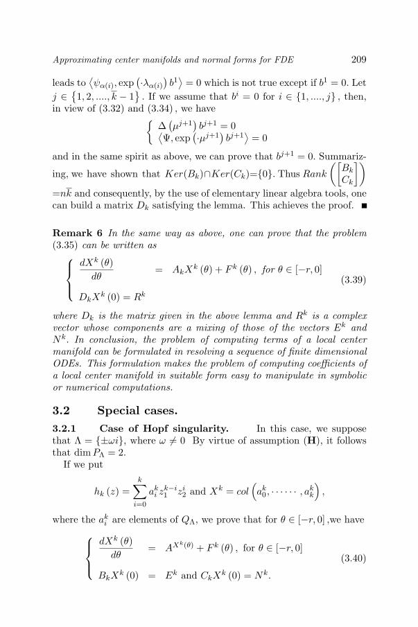
Approximating center manifolds and normal forms for FDE 209
leads to⟨ψα(i), exp
(·λα(i)
)b1⟩
= 0 which is not true except if b1 = 0. Letj ∈
1, 2, ...., k − 1
. If we assume that bi = 0 for i ∈ 1, ...., j , then,
in view of (3.32) and (3.34) , we have∆(µj+1
)bj+1 = 0⟨
Ψ, exp(·µj+1
)bj+1
⟩= 0
and in the same spirit as above, we can prove that bj+1 = 0. Summariz-
ing, we have shown that Ker(Bk)∩Ker(Ck)=0. Thus Rank
([Bk
Ck
])
=nk and consequently, by the use of elementary linear algebra tools, onecan build a matrix Dk satisfying the lemma. This achieves the proof.
Remark 6 In the same way as above, one can prove that the problem(3.35) can be written as
dXk (θ)dθ
= AkXk (θ) + F k (θ) , for θ ∈ [−r, 0]
DkXk (0) = Rk
(3.39)
where Dk is the matrix given in the above lemma and Rk is a complexvector whose components are a mixing of those of the vectors Ek andNk. In conclusion, the problem of computing terms of a local centermanifold can be formulated in resolving a sequence of finite dimensionalODEs. This formulation makes the problem of computing coefficients ofa local center manifold in suitable form easy to manipulate in symbolicor numerical computations.
3.2 Special cases.3.2.1 Case of Hopf singularity. In this case, we supposethat Λ = ±ωi, where ω = 0 By virtue of assumption (H), it followsthat dimPΛ = 2.
If we put
hk (z) =k∑
i=0
aki z
k−i1 zi
2 and Xk = col(ak
0, · · · · · · , akk
),
where the aki are elements of QΛ, we prove that for θ ∈ [−r, 0] ,we have
dXk (θ)dθ
= AXk(θ) + F k (θ) , for θ ∈ [−r, 0]
BkXk (0) = Ek and CkX
k (0) = Nk.
(3.40)

210 DELAY DIFFERENTIAL EQUATIONS
where
Ak =
−kiωIRn 0 0 · · · · · · 0
0 −(k − 2)iωIRn 0. . .
...
0 0. . . . . . . . .
......
. . . . . . . . . . . . 0...
. . . . . . (k − 2)iωIRn 00 · · · · · · 0 0 kiωIRn
,
Bk = Diag (∆(−(k − 2j))iω), , j ∈ 0, · · · , k)and
Ck = Diag (〈Ψ, exp(−(k − 2j))iω)IRn〉 , , j ∈ 0, · · · , k) .
3.2.2 The case of Bogdanov -Takens singularity.. In thiscase, we assume that zero is a double eigenvalue: Λ = 0, 0, whichensures the existence of a center manifold associated with (2.1). Byvirtue of assumption (H), it follows that dimPΛ = 2.
If we put
hk (z) =k∑
i=0
aki z
k−i1 zi
2 and Xk = col(ak
0, · · · · · · , akk
),
where the aki are elements of QΛ,then for θ ∈ [−r, 0] , we have
dXk (θ)dθ
= AkXk (θ) + F k (θ) , for θ ∈ [−r, 0]
BkXk (0) = Ek and CkX
k (0) = Nk.
where
Ak =
0 0 0 · · · · · · 0
kIRn 0 0. . .
...
0 (k − 1) IRn 0. . . . . .
......
. . . . . . . . . . . . 0...
. . . . . . . . . 00 · · · · · · 0 IRn 0
,

Approximating center manifolds and normal forms for FDE 211
and Bk is a consequence of the following lemma:
Lemma 29 The exponential matrix exp(θAk) is given by
exp(θAk) =
Ck0 IRn 0 · · · · · · 0
θCk1 IRn Ck−1
0 IRn. . .
...... θCk−1
1
. . . . . ....
......
. . . 0θkCk
k IRn θk−1Ck−1k−1IRn · · · · · · C0
0IRn
Proof : The matrix Ak is nilpotent. So, it is easy to verify that
exp(θAk) =k∑
m=0
θm (Ak)m
m!.
In a recursive way, one can easily prove that (Ak)m = (αijIRn)1≤ij≤n(k+1) ,
where
αij =
m!Ck−j+1m , if i− j = k
0 , if i− j = k.
which completes the proof of the lemma .By using the above lemma, one can see that
Bk =
Ck0 ∆ (0) 0 · · · · · · 0
Ck1 ∆(1) (0) Ck−1
0 ∆ (0)...
... Ck−11 ∆(1) (0)
. . ....
......
. . . 0Ck
k∆(k) (0) Ck−1k−1∆(k−1) (0) · · · · · · C0
0∆ (0)
.
Example.In this section we consider as an application of our computational
scheme an example treated by Hale and Huang [56], where, in view ofthe study of qualitative structure of the flow on the center manifold,the authors need more precise information about a center manifold. Inparticular, they need to know its Taylor expansion up to the secondorder terms. It is a singularly perturbed delay equation given by
εx′ (t) = −x (t) + f (x (t− 1) , λ) , (3.41)
where ε is a real positive number assumed to be small, λ is a real para-meter and f is an element of Ck (R, R) , k ≥ 3, more specifically
f (x, λ) = − (1 + λ) x + ax2 + bx3 + o(x3), for some a, b ∈ R.

212 DELAY DIFFERENTIAL EQUATIONS
With the change of variables
w1 (t) = x (−εrt) and w2 (t) = x (−εrt + 1 + εr) ,
the equation (3.41) reads
dw1
dt= rw1 (t)− rf (w2 (t− 1) , λ)
dw2
dt= rw2 (t)− rf (w1 (t− 1) , λ) .
(3.42)
If r = 1 and λ = 0, then, the characteristic equation associated to (3.42)is
(µ− 1)2 − e−2µ = 0, for µ ∈ C.
The above equation has zero as a double root and the remaining rootshave a negative real part. This ensures the existence of a two dimensionalcenter manifold associated to the equation (3.42) with (r, λ) = (1, 0)
Throughout this section we use the notation presented in section 2for the equation (3.42) with r = 1 and λ = 0. Base of PΛ and QΛ arerespectively
Φ =[−1 −1
3 − θ1 1
3 + θ
]and Ψ =
[s −s−1 1
], for (θ, s) ∈ [−1, 0]×[0, 1] .
It is easy to verify that 〈Ψ, Φ〉 = IR2 , and
AΦ = ΦB, with B =[
0 10 0
].
In view of the assumed smoothness on the function f, equation (3.42)has a local center manifold, at least of class C3, and
h (ξ) = a20ξ
21+a2
1ξ1ξ2+a22ξ
22+χ (ξ) , for some a2
i ∈ QΛ and χ (ξ) = o(|ξ|2)
.
Put X2 = col(a2
0, a21, a
22
). We showed in subsubsection 3.2.1 that the
computation of X2 can be obtained by solving the differential equation
dX2 (θ)dθ
= A2X2 (θ) + F 2 (θ) , for θ ∈ [−r, 0]
B2X2 (0) = E2 and C2X
2 (0) = N2,
(3.43)

Approximating center manifolds and normal forms for FDE 213
where B2 is the 6× 6 real matrix given by
B2 =
−1 −1 0 0 0 0−1 −1 0 0 0 02 2 −1 −1 0 02 2 −1 −1 0 00 −1 1 1 −1 −1−1 0 1 1 −1 −1
.
Now, we will consider the computation of the parameters of the abovesystem. According to relation (3.23) we have F2 (ξ) (θ) = 0, for θ ∈[−1, 0] . So, F 2 (θ) = 0, for θ ∈ [−1, 0] and as a consequence, we haveN2 = −
⟨Ψ, S2
⟩= 0. Moreover, the relation (3.30) leads to E2 =
col
(−a,−a,
4a
3,4a
3,−4a
9,−4a
9
). On the other hand, by Lemma 29, it
is easy to see that the 6× 6 real matrix G2 is given by
C2 = 〈Ψ, exp (·A2)〉 =
−12
12 0 0 0 0
0 0 0 0 0 013
−13
−12
12 0 0
−1 1 0 0 0 0−112
112
16
−16
−12
12
13
−13
−12
12 0 0
then by replacing the first (resp, the third) line of B2 by the first (resp, bythe third) line of the matrix C2, the boundary condition C2X
2 (0) = N2
and B2X2 (0) = E2 imply that X2(0) is given in the unique way by
X2 (0) = col
(a
2,a
2,a
3,a
3,11a
36,11a
36
)
and for θ ∈ [−1, 0] , we have
a20 (θ) =
a
2
[1
1
], a2
1 (θ) = a
(θ +
1
3
)[1
1
], a2
2 (θ) = a
(θ2
2+
θ
3+
11
36
)[1
1
].
This confirms the result established Hale and Huang in [56].
4. Computational scheme of Normal FormsIn this section, we present an algorithm for computing normal forms
for FDEs. In the context of ODEs, the key idea is based on comput-ing a change of variables that allows us to transform the original ODEinto an equation with a simpler analytic expression. In this section, we

214 DELAY DIFFERENTIAL EQUATIONS
will be concerned with developing, in an algorithmic way, the notion ofnormal forms for FDEs of the form (2.1) . Our approach is shared outin two shutters. In the first subsection, we assume that a local centermanifold is known and we deal with developing, in conventional way, acomputational scheme of normal form for the ODE (2.9) representingthe restriction of the semi-flow generated by (2.1). In the second subsec-tion, we deal with the equation (2.1) as an abstract infinite dimensionalODE of the form (2.8) ; our method consists in elaborating a schemeof computing nonlinear transformations that greatly simplify the (2.8) ,and we will show that this scheme leads us to simpler infinite dimen-sional ODE which coincides with the normal form of (2.1) (in the senseof definition presented in [44]).
4.1 Normal form construction of the reducedsystem
Let h be a mapping from Rm into QΛ whose graph is a local centermanifold associated with the equation (2.1) . In the previous section, wehave elaborated an algorithmic procedure allowing us to compute at anyorder k the terms of the Taylor expansion of h. Note that, in general, it isthe most information that can extracted from h with the impossibility ofobtaining the closed form. Without loss of generality h may be assumedin the form
h =∑i≥2
hi.
The flow of the FDE (2.1), on this local center manifold is described bythe following m-dimensional ODE
•x = Bx + G (x) , (4.44)
where G (x) = Ψ (0)H (x) . If we assume that (hi)i≥2 are already com-puted, then terms of the ODE (4.44) are known at any order. In otherwords, if G =
∑i≥2 Gi then Gi is known for all i ≥ 2 once (hi)i≥2 are
founded.Consider a nonlinear transformation of the form
x = x + V (x) (4.45)
where V be a mapping from Rm into Rm such that V (0) = 0, DV (0) =0. Assume that the effects of the above change of variables on the reducedsystem (4.46) is of the form
•x = Bx + F (x) . (4.46)

Approximating center manifolds and normal forms for FDE 215
Our main goal now is to develop an algorithmic scheme providing uswith adequate nonlinear transformations V that transform (2.6) intoa simpler equation (4.46) (ie. the nonlinearity F is simpler than H).Without loss of generality, we put
V =∑i≥2
Vi and F =∑i≥2
Fi.
In the sequel, we will deal with developing a the recursive efficient ap-proach for computing the kth order normal form Fk and the kth ordernonlinear transformation Vk in terms of (Gi)2≤i≤k as well as the terms(Fi)2≤i≤k−1 already computed. We start by the following Definition:
Definition 35 Let j ≥ 2. We denote by M1j the operator defined by
(M1
j p)(x) = Dp (x)Bx−Bp (x) ,
for all p ∈ V mj (Rm) .
The operators M1j , defined above, are exactly the Lie brackets that
appear in computing normal forms for finite dimensional ODEs. It iswell known that the space V m
j (Rm) may be decomposed as
V mj (Rm) = Im
(M1
j
)⊕ Im
(M1
j
)c (4.47)
where the complementary space Im(M1
j
)cis not uniquely determined.
Let P j be the projection associated with the above decomposition. Ifwe choose bases for Im
(M1
j
)and Im
(M1
j
)c, then, each element q of
V mj (Rm) can be split into two parts P jq and
(I − P j
)q: P jq can be
spanned by the basis of Im(M1
j
)and
(I − P j
)q by that of Im
(M1
k
)c.
Theorem 4 Fix k ≥ 2. Then, the recursive formula for computing thecoefficients of the normal form associated to the decomposition (4.47) isgiven by
Fk (x) = Gk (x)−(M1
kVk
)(x)
+∑k−1
i=2 DGk+1−i (x) Vi (x)−DVi (x) Fk+1−i (x)+∑[ k
2 ]j=2
1j!
∑k−ji=j DjGi (x)
∑l1+l2+...+lj=k−(i−j) Vl1Vl2 ...Vlj
(x) .
(4.48)
Proof. Substituting the change of variables (4.45) into (4.44) resultsin
Bx +∑k≥2
Gk (x) = [I + DV (x)]
Bx +
∑k≥2
Fk (x)
,

216 DELAY DIFFERENTIAL EQUATIONS
which can be rearranged as∑
k≥2 Fk (x) =∑
k≥2 Gk (x + V (x)) +∑
k≥2 BVk (x)
−∑
k≥2 DVk (x) Bx−[∑
k≥2 DVk (x)] [∑
k≥2 Fk (x)]
Then we use Taylor expansion of Gk (x + V (x)) near V = 0 to rewritethe above equation as
∑k≥2 Fk (x) =
∑k≥2 Gk (x) +
∑k≥2 DGk (x)
(∑j≥2 Vj (x)
)
+∑
k≥2
(M1
kVk
)(x)−
[∑k≥2 DVk (x)
] [∑k≥2 Fk (x)
]
+∑
k≥2
(∑j≥2
1j!D
jGk (x)(∑
l≥2 Vl (x))j)
.
Finally comparing terms degree k in the above equation yields the for-mula (4.48). This achieves the proof of the Theorem.
The formula (3.23) given in the above theorem can be rewritten in acompact form
Fk = Gk −M1j Vk, (4.49)
where
Gk (x) = Gk (x) +∑k−1
i=2 DGk+1−i (x)Vi (x)−DVi (x)Fk+1−i (x)+∑k
j=21j!
∑k+ji=j DjGi (x)
∑l1+l2+...+lj=k−(i−j) Vl1Vl2 ...Vlj
(x)
Then, by virtue of (4.49) and (4.47), one can compute an adequatenonlinear transformation Vk such that
M1kVk = P kGk, (4.50)
and which leads us to
Fk =(I − P k
)Gk. (4.51)
In other words, we can find a change of variables that affect the reducedsystem by taking away nonlinear terms (called non resonant terms) thatare in the range subspaces Im
(M1
k
)and conserving only terms (called
resonant terms) that are in the complementary subspace Im(M1
k
)c.
Remark 7 It has been observed that the subspace Im(M1
k
)c is notuniquely determined. Moreover, according to the equations (4.50) and(4.51) , one can note that the nonlinear transformation Vk depends onthe choice of Im
(M1
k
)c. Consequently the normal forms are not unique.In applications, we choose a suitable complementary space to the situa-tion to be handled.

Approximating center manifolds and normal forms for FDE 217
Remark 8 In view of the above Theorem, it is noted that the kth orderterm Fk of the normal form depends upon the known of (Fj)2≤j≤k−1 andthe results (Vj)2≤j≤k as well as (Gj)2≤j≤k−1 . However, it has observedfrom the Proposition (34) that the homogeneous polynomial Gj can begiven in terms of (hi)2≤i≤j−1 . Hence, in order to present the completescheme for computing normal forms for (2.6) , we must take into ac-count the algorithm developed in section 3 and which provides us withhomogeneous parts of the mapping h. As a consequence, the completescheme for computing normal forms for (2.6) should be a combinationof the formulae (3.21) , (3.39) and (3.23) .
In order to save computational time and computer memory, the follow-ing Theorem illustrates another approach that combines center manifoldand normal forms schemes into one step to simultaneously obtain a com-pact form illustrating the close relationship between the normal formsF , the associated nonlinear transformations V, a local center manifold hand the coefficients of the original FDE (2.1) .
Theorem 5 Effect the reduced system (2.9) with a nonlinear transfor-mation of the form (4.45) . So, if x is a solution of the equation ( 2.1)then F and V satisfy
DV (x) Bx−BV (x) = Ψ (0) f(Φ [x + V (x)] + h (x)
)−DV (x) F (x)−F (x) (4.52)
and
Dh (x)B−A1h (x) = (I − π) X0f(Φ [x + V (x)] + h (x)
)−Dh (x) F (x) ,
(4.53)where h (x) = h (x + V (x)) .
Proof. Substituting the nonlinear transformation (4.45) into (2.6)results in
[I + DV (x)]•x = Bx + BV (x) + f1 (x) ,
where f1 (x) = Ψ (0) f(Φ [x + V (x)] + h (x)
). So, in view of (FN1) it
follows that
[I + DV (x)] [Bx + F (x)] = Bx + BV (x) + f1 (x) ,
which can be rearranged as
DV (x)Bx−BV (x) = f1 (x)−DV (x)F (x)− F (x) .
This gives the relation (4.52) . To prove (4.53) , we need the followinglemma:
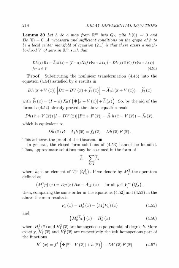
218 DELAY DIFFERENTIAL EQUATIONS
Lemma 30 Let h be a map from Rm into QΛ with h (0) = 0 and
Dh (0) = 0. A necessary and sufficient conditions on the graph of h tobe a local center manifold of equation (2.1) is that there exists a neigh-borhood V of zero in R
m such that
Dh (z) Bz − A1h (z) = (I − π) X0f (Φz + h (z)) − Dh (z) Ψ (0) f (Φz + h (z))
for z ∈ V (4.54)
Proof. Substituting the nonlinear transformation (4.45) into theequation (4.54) satisfied by h results in
Dh (x + V (x))[Bx + BV (x) + f1 (x)
]− A1h (x + V (x)) = f2 (x)
with f2 (x) = (I − π) X0f(Φ [x + V (x)] + h (x)
). So, by the aid of the
formula (4.52) already proved, the above equation reads
Dh (x + V (x)) [I + DV (x)] [Bx + F (x)]− A1h (x + V (x)) = f2 (x) ,
which is equivalent to
Dh (x)B − A1h (x) = f2 (x)−Dh (x)F (x) .
This achieves the proof of the theorem.In general, the closed form solutions of (4.53) cannot be founded.
Thus, approximate solutions may be assumed in the form of
h =∑i≥2
hi
where hi is an element of V mi
(Q1
Λ
). If we denote by M2
j the operatorsdefined as(
M2j p)(x) = Dp (x) Bx− A1p (x) for all p ∈ V m
j
(Q1
Λ
),
then, comparing the same order in the equations (4.52) and (4.53) in theabove theorem results in
Fk (x) = H1k (x)−
(M1
kVk
)(x) (4.55)
and (M2
k hk
)(x) = H2
k (x) (4.56)
where H1k (x) and H2
k (x) are homogeneous polynomial of degree k. Moreexactly, H1
k (x) and H2k (x) are respectively the kth homogenous part of
the functions
H1 (x) = f1(Φ [x + V (x)] + h (x)
)−DV (x)F (x) (4.57)

Approximating center manifolds and normal forms for FDE 219
and
H2 (x) = f2(Φ [x + V (x)] + h (x)
)−Dh (x)F (x) , (4.58)
where f1 (φ) = Ψ (0) f (φ) and f2 (φ) = (I − π) X0f (φ) , for all φ ∈ C.
It is easy to see that H1k = Hk for all k ≥ 2. An exact formula of H1
k (x)and H2
k (x) is given in the following result.
Theorem 6 The recursive formula deriving H1k (x) and H2
k (x) is givenby
H1k (x) = f1
k (Φx) +∑k−1
i=2
Df1
k+1−i (Φx) Wi (x) − DVi (x) Fk+1−i (x)
+∑[ k
2 ]j=2
1j!
∑k−ji=j Djf1
i (Φx)∑
l1+l2+...+lj=k−(i−j) Wl1Wl2 ...Wlj
(x)
and
H2k (x) = f2
k (Φx) +∑k−1
i=2
Df2
k+1−i (Φx) Wi (x) + Dhi (x) Fk+1−i (x)
+∑[ k
2 ]j=2
1j!
∑k−ji=j Djf2
i (Φx)∑
l1+l2+...+lj=k−(i−j) Wl1Wl2 ...Wlj
(x)
,
where Wl = ΦVl + hl for all l ≥ 2.
Proof. In the same spirit of the the proof of the theorem () , one caneasily obtain the above relations.
The above result illustrates clearly how the elements H1k (x) and H2
k (x)
depend into the terms (Vi)2≤i≤k−1 and(hi
)2≤i≤k−1
. So if we assume
that the lower order terms in V and h are already computed, then, inorder to compute an adequate nonlinear transformation Vk that greatlysimplifies the reduced system, we proceed in the following way: We con-sider the equation (4.55) , then, by the aid of a decomposition of theform (4.47) of the space V m
j (Rm) , the homogeneous polynomial H1k (x)
is spliced into two parts the resonant and the non resonant one. Remov-ing non resonant terms and letting resonant terms results in
M1kVk = P kH1
k and Fk =(I − P k
)H1
k .

220 DELAY DIFFERENTIAL EQUATIONS
Remark 9 One can ask a question about the usefulness of the secondequation (4.56) of the scheme. In fact, once H1
k is known, the equation(4.56) will be needed for computing the kth order term hk which allowsus to pass to the next step k + 1 where the computation of the (k + 1)thorder normal form Fk+1 and the (k + 1)th order nonlinear transforma-tion as well as hk+1. In conclusion, solving equation (4.56) is necessaryfor passing from a step to step.
Let us now consider the equation (4.56) . In view of the definition ofh and the formula (4.57) one can easily observe that hk and H2
k arerespectively elements of V m
k
(Q1
Λ
)and V m
k (Ker (π)) . So, according tothe notation presented in section 3, polynomials hk and H2
k are writtenas
hk (x) =k∑
i=1
bki x
qiand H2
k (x) =k∑
i=1
cki x
qi+ X0
k∑i=1
αki x
qi,
where the coefficients(bki
)1≤i≤k
,(cki
)1≤i≤k
and(αk
i
)1≤i≤k
are respec-tively elements of Q1
Λ, Ker (π) and Rn. It is noted that, from the factthat H2
k ∈ V mk (Ker (π)) , the coefficients ck
i and αki should satisfy the
relation cki = ΦΨ (0)αk
i for i = 1, .., k. Put Xk = col(bk1, b
k2, ..., b
kk
)and
F k = col(ck1, c
k2, ..., c
kk
). Identifying the two sides of the equation (4.56)
according the canonical basis
xqi: i = 1, .., k
leads us to
dXk (θ)dθ
= AkXk (θ) + F k (θ) , for θ ∈ [−r, 0]
dXk (0)dθ
− L(Xk)
= Mk Xk ∈ (QΛ)k
where Mk = col(αk
1 , αk2 , ..., α
kk
). Then, if we combine the adjoint bilin-
ear form (cf. section 2) and the variation of constant formula tools, Theabove problem reads
dXk (θ)dθ
= AkXk (θ) + F k (θ) , for θ ∈ [−r, 0]
BkXk (0) = Ek and CkX
k (0) = Nk
whereNk = −
⟨Ψ, Sk
⟩(4.59)

Approximating center manifolds and normal forms for FDE 221
andEk = Mk − F k (0)− LSk (4.60)
with
Sk =∫ θ
0exp ((θ − s) Ak)F k (s) ds
Finally, we have the following result which provides us with the algorithmof computing coefficients
(bki
)1≤i≤k
in terms of(cki
)1≤i≤k
and(αk
i
)1≤i≤k
.
Proposition 35 Let Ak and Dk are the matrices appearing in the al-gorithm of approximation of a local center manifold (cf. section 3). Theequation (3.38) is equivalent to
dXk (θ)dθ
= AkXk (θ) + F k (θ) , for θ ∈ [−r, 0]
DkXk (0) = Rk
(4.61)
where Rk is a vector whose components are a mixing of the ones of thevectors Ek and Nk respectively defined in (4.60) and (4.59).
In conclusion, we claim that the sequence of equations (4.55) and(4.61) is all what we need for computing normal formes for the reducedsystem (2.6) at any order.
Remark 10 In the work [44], the authors have been concerned withsolving, at each step, equations similar to (4.55) and (4.56) . In view ofthe difficulties entailed by the operator A1 in the definition of M2
j (j ≥ 2),the authors in [44] have been restricted to the study of the spectrum ofA1. And under non resonance conditions, the authors in [44] proved thatM2
j is nonsingular for all j ≥ 2. However, their derivation does notallow them to compute or at least approximate the inverse of M2
j . Incontrast, the previous result provides us with a suitable form of (4.56)which lends itself to numerical or symbolic computations by means of arecursive process.
4.2 Normal form construction for FDEsIn this subsection, we will be concerned with equation (2.1) , for which
an algorithmic scheme for computing normal forms is derived. In viewof the preliminary section, it is known that equation (2.1) can viewed asan infinite dimensional ODE given by •
x = Bx + f1 (x, y)
•y = A1y + f
2 (x, y)(4.62)

222 DELAY DIFFERENTIAL EQUATIONS
where f1 (x, y) = Ψ (0) f (Φx + y) and f
2 (x, y) = (I − π) X0f (Φx + y) .Effecting the equation (4.62) with nonlinear transformations of the form
x = x + V 1 (x)y = y + V 2 (x) (4.63)
results in •x = Bx + g1 (x, y)•y = A1y + g2 (x, y)
(4.64)
Our goal in the sequel is to develop an iterative procedure for find-ing adequate transformations V 1 and V 2 that greatly simplify equation(4.62) . As has been defined in [44], the transformed equation (4.64) as-sociated to that change of variables is called normal form of (2.1). Wefirst start by stating the following Theorem that illustrates us how, theabove change of variables (4.63) , affects equation (4.62) .
Theorem 7 Effecting the equation (4.62) with the change of variables(4.45) results in equation of the form(4.64) with g1 and g2 satisfying
g1 (x, y) = f1 (
x + V 1 (x) , y + V 2 (x))− DV 1 (x) g1 (x, y)−
[DV 1 (x) Bx − BV 1 (x)
](4.65)
and
g2 (x, y) = f2 (
x + V 1 (x) , y + V 2 (x))−DV 2 (x) g1 (x, y)−
[DV 2 (x) Bx − A1V
2 (x)]
(4.66)
Proof. First, differentiating the relations of (4.63) results in •
x =[I + DV 1 (x)
] •x
•y =
•y + DV 2 (x)
•x
So, assuming that the change of variables (4.45) transforms equation(4.62) into equation of the form (FN2) yields
•x =
[I + DV 1 (x)
] [Bx + g1 (x, y)
]•y =
[A1y + g2 (x, y)
]+ DV 2 (x)
[Bx + g1 (x, y)
]
Finally combining the above formula with (4.62) and (4.63) yields equa-tions (4.65) and (4.66) . This ends the proof of the Theorem.
A conventional approach for computing normal forms consists in find-ing adequate nonlinear transformations V 1 and V 2 that provide us, bysubstituting them into equation (4.62) , with a simpler form of the both

Approximating center manifolds and normal forms for FDE 223
of g1 and g2. In general, however, the closed form of V 1 and V 2 respec-tively solutions of (4.65) and (4.66) cannot be founded. Thus, approxi-mate solutions may be assumed in the form of
V 1 =∑i≥2
V 1i and V 2 =
∑i≥2
V 2i .
Our task is then reduced only to the computation terms of the Taylor
expansion respectively of V 1 and V 2. Denote by f1(x, y) and f
2(x, y) re-
spectively the function f2 (
x + V 1 (x) , y + V 2 (x))
andf
2 (x + V 1 (x) , y + V 2 (x)
). So, expanding and comparing the both sides
of equations (4.65) and (4.66) results in
g1k (x, y) =
˜f
1
k (x, y)−(M1
kV 1k
)(x) (4.67)
and
g2k (x, y) =
˜f
2
k (x, y)−(M2
kV 2)(x) (4.68)
where˜f
1
k (x, y) and˜f
2
k (x, y) are respectively the kth order term (with
respect to the arguments x and y) of the functions˜f
1
(x, y) = f1(x, y)−
DV 1 (x) g1 (x, y) and˜f
2
(x, y) = f2(x, y)−DV 2 (x) g1 (x, y) . More pre-
cisely, we have the following proposition:
Theorem 8 The recursive expression of˜f
1
k (x, y) and˜f
2
k (x, y) is givenby
˜f1
k (x, y) = f1k (Φx + y) +
∑k−1i=2
Df1
i (Φx + y) Wk+1−i (x) + DV 1i (x) g1
k+1−i (x, y)
+∑[ k
2 ]j=2
1j!
∑k−ji=j Djf1
i (Φx + y)∑
l1+l2+...+lj=k−(i−j) Wl1Wl2 ...Wlj
(x)
(4.69)
and
˜f2
k (x, y) = f2k (Φx + y) +
∑k−1i=2
Df2
i (Φx + y) Wk+1−i (x) + DV 1i (x) g1
k+1−i (x, y)
+∑[ k
2 ]j=2
1j!
∑k−ji=j Djf2
i (Φx + y)∑
l1+l2+...+lj=k−(i−j) Wl1Wl2 ...Wlj
(x)
(4.70)
where Wl (x) is the homogeneous part of degree l of W (x) = ΦV 1 (x) +V 2 (x) .
Fix y = 0 in formulae (4.67) and (4.68) . Refereing to the results statedin the previous subsection, one can find adequate nonlinear transforma-

224 DELAY DIFFERENTIAL EQUATIONS
tions V 1k and V 2
k satisfying
(M1
kV 1k
)(x) = P k ˜f
1
k (x, 0) (4.71)
g1k (x, 0) =
(I − P k
) ˜f
1
k (x, 0) (4.72)
and (M2
kV 2k
)(x) =
˜f
2
k (x, 0) . (4.73)
And thus g2k (x, 0) = 0. To be explicit, we state the following definition,
similar to the one given in [44], of normal forms for (2.1):
Definition 36 The normal form for (2.1) (or equation (2.7)) relativeto the decomposition (4.47) is an equation of the form
•x = Bx +
∑k≥2 g1
k (x, y)•y = A1y +
∑k≥2 g2
k (x, y)
with g1k and g2
k satisfying (4.71) , (4.72) and (4.73) for all k ≥ 2.
Now, with the aid of the previous Definition, we are in position tostate the following Theorem summarizing the results for the new recur-sive and computationally efficient approach, providing us with terms ofthe normal form for FDEs at any order and the associated nonlineartransformations:
Theorem 9 Consider an FDE of the form (2.1) with non hyperbolicsteady state satisfying the hypothesis (H) . If we consider (2.1) as aninfinite dimensional ODE of the form (2.8) , then there exists formalnonlinear transformations x = x + V 1 (x) and y = y + V 2 (y) such that
•x = Bx +
∑k≥2 g1
k (x, y)•y = A1y +
∑k≥2 g2
k (x, y)(4.74)
with g1k and g2
k satisfying (4.71) , (4.65) , (4.73) and g2k (x, 0) = 0 for x, y
small and k ≥ 2. Moreover, a local center manifold satisfies y = 0 andthe normal form (in the usual sense for ODEs) of the reduced system of(2.1) on this invariant manifold is given by the m-dimensional ODE
•x = Bx + g1 (x, 0) . (4.75)

Approximating center manifolds and normal forms for FDE 225
Proof: After what was done before the statement, one can see thatthe first part of the Theorem is a direct consequence of properties of theoperators M1
k and M2k stated in the previous subsection combined with
the equations (4.71) , (4.65) , (4.73) . Let us to prove the second part ofthe Theorem. This will be done in two steps: First, substituting y = 0into (4.69) results in
˜f
1
k (x, 0) = f1k (Φx) +
∑k−1i=2
Df1
i (Φx) Wk+1−i (x) + DV 1i (x) g1
k+1−i (x)
+∑[ k
2 ]j=2
1j!
∑k−ji=j Djf1
i (Φx)∑
l1+l2+...+lj=k−(i−j) Wl1Wl2 ...Wlj
(x) .
So, if we observe that
H1i (x) = Ψ (0) fi (Φx) for i ≥ 2
then, it follows thatg1k (x, 0) = Fk (x) .
As a consequence, the equation (4.75) is exactly the normal form of thereduced system of (2.1) in the local center manifold considered. In thesecond step, we need to show that y = 0 provides us with this centermanifold. To this end we need the following lemma:
Lemma 31 The equation y = 0 yields the equation of a local invariantcenter manifold of (2.1) .
Proof: Substituting y = 0 in the change of variables (4.63) yields
x = x + V 1 (x)y = V 2 (x) .
(4.76)
So, by applying the implicit functions Theorem to the above equation,one can prove the existence of a function h mapping a neighborhood Vof zero in Rm into Ker (π) such that y = l (x) . This implies that
V 2 (x) = l (x) = l(x + V 1 (x)
). (4.77)
In the other hand, it is known that V 2 (x) is a solution of (4.66) . Thisreads[
DV 2 (x)Bx− A1V2 (x)
]= f
2 (x + V 1 (x) , V 2 (x)
)−DV 2 (x)F (x) .
So, by virtue of (4.77), the above equation can be written as[Dl (x)Bx−
(A1 l)
(x)]
= G (x) , (4.78)

226 DELAY DIFFERENTIAL EQUATIONS
where G (x) = (I − π)X0f(Φ(x + V 1 (x)
), l (x)
)− Dl (x)F (x). To
achieve the proof of the Lemma, we should prove that the kth parts lk (x)and hk (x) respectively of l (x) and h (x) coincide for all k ≥ 2. This willbe done is a recursive way: In one hand, for k = 2, it is noted that l2 (x)and h2 (x) are respectively solutions of
(M2
2 h2
)(x) = (I − π) X0f2 (x)
and(M2
2 l2
)(x) = (I − π) X0f2 (x), and since the operator is nonsingu-
lar then it follows that l2 (x) = h2 (x) . In the other hand, Assuming thatli (x) = hi (x) for 2 ≤ i ≤ k − 1 results in
H2k (x) = Gk (x) ,
where Gk (x) is the homogeneous part of degree k of the function G (x)defined above. Thus, combining (4.78) and (4.56) leads to lk (x) =hk (x) . This ends the proof of the Theorem.

Chapter 7
NORMAL FORMS AND BIFURCATIONSFOR DELAY DIFFERENTIAL EQUATIONS
T. FariaDepartamento de Matematica,Faculdade de Ciencias, and CMAF,Universidade de LisboaCampo Grande 1749-016 [email protected]
1. IntroductionThe key idea of the normal form (n.f.) technique is to transform a
nonlinear differential equation into an equation with a simpler analyticexpression, called a normal form, which has the same qualitative behav-iour of the original equation. In the framework of ordinary differentialequations (ODEs), this idea is very old, going back to the late XIXcentury with the works of Poincare on Celestial Mechanics, and earlyXX century with the works of Liapunov and Birkhoff. More recently(1970’s), Bibikov and Br’juno gave significant contributions to the field.
Before developing a normal form theory for delay differential equa-tions (DDEs), a brief explanation of the method for ODEs is given.
Consider an autonomous nonlinear ODE in Rn with an equilibrium
at zero,
x(t) = Bx + f(x) (1.1)
where B is an n × n constant matrix, f(0) = 0, Df(0) = 0 and f ∈Ck(k ≥ 2). The application of the method of n.f. is of interest mostlyin the case of a non-hyperbolic equilibrium x = 0. In fact, if x = 0is a hyperbolic equilibrium, i.e., all the eigenvalues of B have nonzeroreal parts, the theorem of Hartman-Grobman assures that, around theorigin, Eq. (1.1) is topologically equivalent to the linearization x = Bx.
© 2006 Springer.
227
O. Arino et al. (eds.), Delay Differential Equations and Applications, 227–282.

DELAY DIFFERENTIAL EQUATIONS
Write the Taylor formula for f ,
f(x) =k∑
j=2
1j!
fj(x) + o(|x|k),
where fj ∈ V nj (Rn) is the j-th Frechet derivative of f at zero. Here, we
use the notation V nj (Y ) to denote the space of homogeneous polynomials
of degree j in n variables x = (x1, . . . , xn) ∈ Rn, with coefficients in Y ,
for Y a Banach space.The method of n.f. consists of a recursive process of changes of
variables, such that, at each step j, 2 ≤ j ≤ k, all the nonrelevant termsof order j are eliminated from the equation. At a step j, assume thatsteps of orders 2, . . . , j − 1 have already been performed, leading to
x = Bx +12g2(x) + · · ·+ 1
(j − 1)!gj−1(x) +
1j!
fj(x) + h.o.t,
where 1j! fj(x) are the terms of order j obtained after the changes of
variables in previous steps, and h.o.t stands for higher order terms. Achange of variables of the form
x = x +1j!
Uj(x), with Uj ∈ V nj (Rn), (1.2)
is then applied to the above equation, transforming it into
˙x = Bx +12g2(x) + · · ·+ 1
j!gj(x) + h.o.t, x ∈ R
n, (1.3)
with the new terms of order j given by
gj = fj − [B, Uj ],
where [B, Uj ] is the Lie bracket
[B, Uj ](x) = DUj(x)Bx−BUj(x).
The operators associated with these changes of variables,
Mj : V nj (Rn) → V n
j (Rn), MjU = [B, U ], (1.4)
permit to write gj = fj−MjUj . Hence, one can choose Uj in such a waythat
gj ∈ Im (Mj)c,
228

Normal Forms And Bifurcations For DDE
where Im (Mj)c is a complementary space (in general not uniquely de-termined) of Im (Mj). Let Pj : V n
j (Rn) → Im (Mj) be the canonicalprojection associated with a decomposition
V nj (Rn) = Im (Mj)⊕ Im (Mj)c. (1.5)
In order to have
gj = ProjIm (Mj)c fj = (I − Pj)fj , (1.6)
Uj must be chosen so that MjUj = Pj fj , thus
Uj = (Mj)−1Pj fj , (1.7)
where (Mj)−1 is a right inverse of Mj , associated with a decompositionV n
j (Rn) = Ker (Mj) ⊕ Ker (Mj)c. For gj , Uj defined by (1.6), (1.7),Eq. (1.3) is called a normal form for Eq. (1.1), up to j order terms.The terms 1
j!gj(x) ∈ Im (Mj)c that cannot be eliminated from (1.1) arecalled resonant terms of order j.
Consider now an equation (1.1) in the form
x = Bx + f1(x, y)y = Cy + f2(x, y), x ∈ R
p, y ∈ Rm,
(1.8)
where B is a p×p matrix, C is an m×m matrix, p+m = n, Reλ(B) =0, Re λ(C) = 0, f1 : R
n → Rp, f2 : R
n → Rm are Ck functions (k ≥ 2)
such that f1(0, 0) = 0, f2(0, 0) = 0, Df1(0, 0) = 0, Df2(0, 0) = 0. Thecentre manifold theorem tells us that there is a centre manifold W c =(x, y) : y = h(x), x ∈ V , where V is a neighbourhood of 0 ∈ R
p,tangent at zero to the centre space R
p for the linearization of (1.8), andthat the qualitative behaviour of the flow near zero is determined by itsbehaviour on the centre manifold.
In order to apply the normal form procedure to the equation for theflow on the centre manifold of (1.8), there are two possible approaches.We can actually compute recursively the function h(x) = 1
2h2(x) + · · ·giving the equation of W c (see e.g. [24]), and therefore write the equationfor the flow on such manifold:
x = Bx + f1(x, h(x)). (1.9)
After this first step, the method of n.f. described above is applied tocompute a n.f. for (1.9). This approach is not very efficient, since itrequires to compute the centre manifold beforehand.
229

DELAY DIFFERENTIAL EQUATIONS
Another procedure ([29, Chapter 12]) is based on the idea that,at each step j, a change of variables is used to project the originalequation (1.8) on the centre manifold and, simultaneously, to eliminatethe non-resonant terms of order j from the equation giving the flowon the centre manifold. This is achieved by considering a sequence ofchange of variables
x = x +1j!
U1j (x), y = y +
1j!
U2j (x), (1.10)
where U1j ∈ V p
j (Rp), U2j ∈ V p
j (Rm). Following the procedure describedabove, where now the change of variables (1.2) is replaced by (1.10),after steps j = 2, . . . , k Eq. (1.8) is transformed into an equation in theform
x = Bx + g12(x, y) + · · ·+ 1
k!g1k(x, y) + h.o.t,
y = Cy + g22(x, y) + · · ·+ 1
k!g2k(x, y) + h.o.t, , x ∈ R
p, y ∈ Rm,(1.11)
where the new terms gj = (g1j , g
2j ) of orders j, j = 2, . . . , k, are given by
g1j = f1
j −M1j U1
j , g2j = f2
j −M2j U2
j ,
with the operators M1j defined as before, M1
j U = [B, U ], and
M2j : V p
j (Rm) → V pj (Rm), (M2
j U)(x) = DU(x)Bx− CU(x). (1.12)
Remark 1.1. This latter procedure provides a general setting to benaturally extended to infinite-dimensional spaces, such as the naturalphase space for a retarded functional differential equation (FDE) in R
n.However, some difficulties arise in working in an infinite-dimensionalphase space. First of all, it is not clear how to decompose the linear partof an FDE in R
n so that it can be written as (1.8), where x ∈ Rp ≡ P , for
P the centre space for its linearization at zero, and y in a complementaryspace P c for P . Note that the linearization of (1.8) is given by the system
x= Bx
y= Cy, x ∈ Rp, y ∈ R
m.(1.13)
Clearly, a complementary space P c for P can be obtained by using theformal adjoint theory for linear DDEs in R
n (cf. [58]), although thisis not sufficient to decompose a linear DDE into a decoupled system oflinear DDEs similar to (1.13). A second difficulty comes from the factthat the operator M2
j in (1.12) will be defined in an infinite-dimensionalspace V p
j (P c). Hence a decomposition similar to (1.5) is not obvious.
230

Normal Forms And Bifurcations For DDE
Remark 1.2. For the sake of exposition, in general formal Taylor serieswill be considered. Even if f is analytic, the function g = 1
2g2+ 13!g3+· · ·
in the n.f. is not necessarily analytic. However, in applications this is nota problem, since we are mainly interested in applying n.f. to the study ofsingularities with possible bifurcations that are generically determinedup to a finite jet.
2. Normal Forms for FDEs in FiniteDimensional Spaces
In the next sections, we refer the reader to [58] for notation andgeneral results on the theory of retarded FDEs in finite dimensionalspaces.
Consider autonomous semilinear FDEs of retarded type in Rn (or
Cn) and with an equilibrium point at the origin,
u(t) = L(ut) + F (ut) (t ≥ 0), (2.1)
where r > 0, C := C([−r, 0]; Rn) is the Banach space of continuousmappings from [−r, 0] to R
n equipped with the sup norm, ut ∈ C isdefined by ut(θ) = u(t+θ) for θ ∈ [−r, 0], L : C → R
n is a bounded linearoperator, and F is a Ck function (k ≥ 2), with F (0) = 0, DF (0) = 0.
Consider also the linearized equation at zero,
u(t) = L(ut), (2.2)
and its characteristic equation
det∆(λ) = 0, ∆(λ) := L(eλ·I)− λI,
where I is the n×n identity matrix. Let A be the infinitesimal generatorfor the C0-semigroup defined by the flow of (2.2),
A : D(A) ⊂ C → C, Aϕ = ϕ,
where D(A) = ϕ ∈ C : ϕ ∈ C, ϕ(0) = L(ϕ). We recall that A has onlythe point spectrum, and
σ(A) = σP (A) = λ ∈ C : det∆(λ) = 0.
2.1 Preliminaries
For Rn∗ the n-dimensional vector space of row vectors, define C∗ =
C([0, r]; Rn∗), and the formal duality (·, ·) in C∗ × C,
(ψ, ϕ) = ψ(0)ϕ(0)−∫ 0
−r
∫ θ
0ψ(ξ − θ)dη(θ)ϕ(ξ)dξ, ψ ∈ C∗, ϕ ∈ C,
231

DELAY DIFFERENTIAL EQUATIONS
where η : [−r, 0]→ Rn×R
n is a function of bounded variation such that
L(ϕ) =∫ 0
−rdη(θ)ϕ(θ).
The formal adjoint operator A∗ of A is defined as the infinitesimal gen-erator for the solution operator of the adjoint equation in C∗,
y(t) = −∫ 0
−ry(t− θ)dη(θ), t ≤ 0.
Fix a nonempty finite set Λ = λ1, . . . , λs ⊂ σ(A). Using theformal adjoint theory of Hale (see [58, Chapter 7]), the phase space Cis decomposed by Λ as
C = P ⊕Q,
where P is the generalized eigenspace associated with the eigenvaluesin Λ, Q = ϕ ∈ C : (ψ, ϕ) = 0 for all ψ ∈ P ∗, and the dual spaceP ∗ is the generalized eigenspace for A∗ associated with the eigenvaluesin Λ. For dual bases Φ and Ψ of P and P ∗ respectively, such that(Ψ, Φ) = Ip, p = dimP , there exists a p×p real matrix B with σ(B) = Λ,that satisfies simultaneously Φ = ΦB and −Ψ = BΨ.
2.2 The enlarged phase space
To develop a normal form theory for FDEs, first it is necessary toenlarge the phase space C in such a way that (2.1) is written as anabstract ODE. An adequate phase space to accomplish this is the spaceBC (see [30, 44, 45]) defined by
BC := ψ : [−r, 0]→ Rn | ψ is continuous on [−r, 0),∃ lim
θ→0−ψ(θ) ∈ R
n,
with the sup norm. The elements of BC have the form ψ = ϕ+X0α, ϕ ∈C,α ∈ R
n, where
X0(θ) =
0, −r ≤ θ < 0I, θ = 0, (I is the n× n identity matrix),
so that BC is identified with C ×Rn with the norm |ϕ + X0α| = |ϕ|C +
|α|Rn .Let v(t) = ut ∈ C. In BC, Eq. (2.1) takes the form
dvdt (0)= L(v) + F (v)dvdt (θ)= v(θ), for θ ∈ [−r, 0),
232

Normal Forms And Bifurcations For DDE
with the notation dvdθ (θ) = v(θ), θ ∈ [−r, 0]. Define an extension of the
infinitesimal generator A, denoted by A,
A : C1 ⊂ BC → BC, Aϕ = ϕ + X0[L(ϕ)− ϕ(0)],
where D(A) = C1 := ϕ ∈ C | ϕ ∈ C. We then write (2.1) as
dv
dt= Av + X0F (v), (2.3)
which is the abstract ODE in BC associated with (2.1). In a naturalway, we also extend the duality (·, ·)C∗×C to a bilinear form on C∗×BCby defining
(ψ, X0α) = ψ(0)α, ψ ∈ C∗, α ∈ Rn.
The canonical projection of C onto P associated with the decompositionC = P ⊕ Q, ϕ → ϕP = Φ(Ψ, ϕ), is therefore extended to a canonicalprojection
π : BC → P, π(ϕ+X0α) = Φ[(Ψ, ϕ)+Ψ(0)α
], ϕ ∈ C,α ∈ R
n. (2.4)
By using the definition of π and A, and integration by parts, it is easyto prove the following lemma.Lemma 2.1. π is a continuous projection on BC that commutes withA on D(A) = C1.
Since π is a continuous projection, the decomposition C = P ⊕ Qyields a decomposition of BC by Λ as the topological direct sum
BC = P ⊕Ker π. (2.5)
Writing v ∈ C1 according to the above decomposition, v = Φx + y,with x ∈ R
p (p = dim P ), y ∈ C1 ∩Ker π = C1 ∩ Q := Q1, and sinceπA = Aπ in C1, (2.3) becomes
Φdx
dt+
dy
dt= AΦx + Ay + πX0F (Φx + y) + (I − π)X0F (Φx + y)
= Φx + Ay + ΦΨ(0)F (Φx + y) + (I − π)X0F (Φx + y).
Therefore, Eq. (2.3) is decomposed as a system of abstract ODEs inR
p ×Ker π ≡ BC, as
x = Bx + Ψ(0)F (Φx + y)
y = AQ1y + (I − π)X0F (Φx + y), x ∈ Rp, y ∈ Q1,
(2.6)
where AQ1 is the restriction of A to Q1 interpreted as an operator actingin the Banach space Ker π.
233

DELAY DIFFERENTIAL EQUATIONS
Note that the linear part of system (2.6) looks like (1.13), i.e., thefinite dimensional variable x and the infinite dimensional variable y aredecoupled in the linear part of the equation. We also point out thatthe enlarged phase space BC was used by Chow and Mallet-Paret [30]to derive system (2.6). However, since the decomposition (2.5) was notexplicitly given in [30], the definition of the linear operator AQ1 in thesecond equation of (2.6) was not adequate. In fact, the spectrum ofAQ1 plays an important role in the construction of normal forms, so itis crucial to restrict A to a linear operator in the Banach space Ker π.In this setting, we can prove [44] thatLemma 2.2. σ(AQ1) = σP (AQ1) = σ(A) \ Λ.
2.3 Normal form construction
In applications, we are particularly interested in obtaining n.f. forequations giving the flow on centre manifolds. Therefore, and for thesake of exposition, we turn our attention to the case where Λ is the set ofeigenvalues of A on the imaginary axis, Λ = λ ∈ σ(A) : Reλ = 0 = ∅.The centre manifold theorem ([58, Chapter 10] and references therein)assures that there is a p-dimensional invariant manifold for (2.1),
W c = ϕ ∈ C : ϕ = Φx + h(x), for x ∈ V , (2.7)
where V is a neighbourhood of 0 ∈ Rp, which is tangent to the centre
space P for (2.2) at zero. From Eq. (2.6), we write the ODE for theflow on W c as
x = Bx + Ψ(0)F (Φx + h(x)), x ∈ V. (2.8)
The goal now is to develop an algorithm of n.f. which affects si-multaneously the linearization of the centre manifold and reduces theODE (2.8) to a n.f., up to a finite order k. In fact, as we will mention,we can consider any nonempty finite set Λ ⊂ σ(A) for which there isan invariant manifold tangent to P at zero, where P is the generalizedeigenspace of (2.2) associated with the eigenvalues in Λ. In this case, themethod described here is applied to compute a n.f. for the ODE givingthe flow on such manifold.
Consider the formal Taylor expansion of F ,
F (v) =∑j≥2
1j!
Fj(v), v ∈ C,
234

Normal Forms And Bifurcations For DDE
where Fj is jth Frechet derivative of F . Eq. (2.6) becomes
x = Bx +∑
j≥21j!f
1j (x, y)
y = AQ1y +∑
j≥21j!f
2j (x, y), x ∈ R
p, y ∈ Q1,(2.9)
with fj := (f1j , f2
j ), j ≥ 2, defined by
f1j (x, y) = Ψ(0)Fj(Φx + y), f2
j (x, y) = (I − π)X0Fj(Φx + y). (2.10)
As for autonomous ODEs in Rn, n.f. are obtained by a recursive
process of changes of variables. At a step j, the terms of order j ≥ 2 arecomputed from the terms of the same order and from the terms of lowerorders already computed in previous steps. Assume that steps of orders2, . . . , j − 1 have already been performed, leading to
x = Bx +
∑j−1=2
1!g
1 (x, y) + 1
j! f1j (x, y) + h.o.t.
˙y = AQ1y +∑j−1
=21!g
2 (x, y) + 1
j! f2j (x, y) + h.o.t.,
where we denote by fj = (f1j , f2
j ) the terms of order j in (x, y) obtainedafter the previous transformations of variables. At step j, effect a changeof variables that has the form
(x, y) = (x, y) +1j!
(U1j (x), U2
j (x)), (2.11j)
where x, x ∈ Rp, y, y ∈ Q1 and U1
j : Rp → R
p, U2j : R
p → Q1 are ho-mogeneous polynomials of degree j in x. That is, U1
j ∈ V pj (Rp), U2
j ∈V p
j (Q1), where we adopt the following notation (cf. Section 1): forj, p ∈ N and Y a normed space, V p
j (Y ) denotes the space of homo-geneous polynomials of degree j in p variables, x = (x1, . . . , xp), withcoefficients in Y , V p
j (Y ) = ∑
|q|=j cqxq : q ∈ N
p0, cq ∈ Y , with the norm
|∑
|q|=j cqxq| =
∑|q|=j |cq|Y .
This recursive process transforms (2.9) into the normal form
˙x = Bx +∑
j≥21j!g
1j (x, y)
˙y = AQ1 y +∑
j≥21j!g
2j (x, y),
(2.12)
where gj := (g1j , g
2j ) are the new terms of order j, given by
g1j (x, y) = f1
j (x, y)− [DU1j (x)Bx−BU1
j (x)]
g2j (x, y) = f2
j (x, y)− [DU2j (x)Bx−AQ1(U2
j (x))], j ≥ 2.
235

DELAY DIFFERENTIAL EQUATIONS
Define the operators Mj = (M1j , M2
j ), j ≥ 2, by
M1j : V p
j (Rp) → V pj (Rp), M2
j : V pj (Q1) ⊂ V p
j (Ker π) → V pj (Ker π)
(M1j h1)(x) = Dh1(x)Bx − Bh1(x), (M2
j h2)(x) = Dxh2(x)Bx − AQ1(h2(x)).
(2.13)
With Uj = (U1j , U2
j ), it is clear that
gj(x, y) = fj(x, y) − MjUj(x),
so for y = 0 one can define
gj(x, o) = (I − Pj)fj(x, 0), (2.14)
where I is the identity operator on V pj (Rp) × V p
j (Ker π) and Pj =(P 1
j , P 2j ) is the canonical projection of V p
j (Rp)×V pj (Ker π) onto ImMj .
The operators M1j , defined by the Lie brackets, are the operators
that appear in Section 1 for computing n.f. for finite-dimensional ODEs.The infinite-dimensional part in the transformation formulas is handledthrough the operators M2
j . Clearly, the ranges of M1j , M2
j contain ex-actly the terms that can be removed from the equation, called non-resonant terms. The remaining terms (resonant terms) are in generalnot determined in a unique way, depending on the choices of comple-mentary spaces Im (Mj)c for Im (Mj). We are particularly interested inthe situation of M2
j surjective and one-to-one, j ≥ 2.Theorem 2.3. Assume that the operators M2
j , 2 ≤ j ≤ k, are one-to-one and onto. Let (x, y) = Θ(x, y) = (x, y) + O(|x|k) be the changeof variables obtained after the sequence of transformations (2.11j), 2 ≤j ≤ k. Then, the local centre manifold W c for (2.1) defined in (2.7) istransformed into
Wc = ϕ ∈ C : ϕ = Φx + h(x), for x ∈ V ,
where V is a neighbourhood of 0 ∈ Rp, with
h(x) = o(|x|k).
Consequently the flow on Wc is given by (after dropping the bars)
x = Bx +k∑
j=2
g1j (x, 0) + o(|x|k), x ∈ V , (2.15)
and the change (x, y) = Θ(x, y) can be chosen so that (2.15) is in n.f.(in the usual sense of n.f. for ODEs).
236

Normal Forms And Bifurcations For DDE
Proof. Let Eq. (2.6) be transformed into
˙x = Bx +∑k
j=21j!g
1j (x, y) + h.o.t.
˙y = AQ1 y +∑k
j=21j!g
2j (x, y) + h.o.t.,
(2.16)
through the change (x, y) = Θ(x, y). Write h(x) = 12h2(x) + o(|x|2). For
y = h(x), from (2.16) we get
Dh(x)x = AQ1(h(x)) +12g22(x, h(x)) + O(|x|4).
Using again (2.16), we have
12Dh2(x)[Bx + O(|x|2)] + O(|x|3) =
12AQ1(h2(x)) +
12g22(x, 0) + O(|x|3).
From (2.14), we conclude that g22(x, 0) = 0, because M2
2 is onto. Hence
Dh2(x)Bx−AQ1(h2(x)) = 0,
that is, M22 h2 = 0. Since M2
2 is one-to-one, this implies that h2 = 0, andthus y = o(|x|2). On the other hand, since the operators M1
j coincidewith the operators in the algorithm for computing n.f. for ODEs in R
p,equation
˙x = Bx +12g12(x, 0) + h.o.t
is a n.f. for (2.8) up to second order terms. The rest of the proof followsby induction.
Since A is the infinitesimal generator of a C0-semigroup, it is aclosed operator. This implies that the extension A is also a closed oper-ator. Note that the restriction AQ1 = A|Q1 is an operator acting in theBanach space Ker π, therefore AQ1 is also closed. Thus, it is straightfor-ward to prove that M2
j , j ≥ 2, are closed operators in the Banach spaceV p
j (Ker π), so M2j are one-to-one and onto if and only if 0 ∈ σ(M2
j ).The spectra of the operators M2
j are given in the theorem below.Theorem 2.4. With the above notations,
(i) σP (M2j ) = (q, λ)− µ : µ ∈ σ(A1
Q), q ∈ Dj;(ii) σ(M2
j ) = σP (M2j ),
where: Dj = q ∈ Np0 : |q| = j; |q| = q1 + · · ·+ qp for q = (q1, . . . , qp);
λ = (λ1, . . . , λp) where λ1, . . . , λp are the eigenvalues in Λ, countingmultiplicities; (q, λ) = q1λ1 + · · ·+ qpλp.
Proof. The complete proof of this theorem can be found in [44]. (Seealso [45] for the situation of DDEs with parameters.) Here we give onlya sketch of the proof.
237

DELAY DIFFERENTIAL EQUATIONS
By adapting the algebraic arguments for finite ODEs in [29, Chap-ter 12], one can prove (i). To prove (ii), it is sufficient to show that ifα ∈ σP (M2
j ), then the operator αI −M2j is surjective. In order to prove
this, consider the set Dj with the following order: for q = (q1, . . . , qp)and = (1, . . . , p) in Dj , we say that q < if the first non-zero differ-ence q1− 1, . . . , qp − p is positive. In this order, (j, 0, . . . , 0) is the firstelement in Dj , and (0, . . . , 0, j) is the last element.
Let α ∈ σP (M2j ). From (i), we deduce that µq := (q, λ)−α ∈ ρ(AQ1)
for all q ∈ Dj . Fix g =∑
q∈Djgqx
q ∈ V pj (Ker π). By induction in Dj
ordered as above, for any q ∈ Dj it is possible to construct
h(q) =∑∈Dj
hx
such that[(αI −M2
j )h(q)] = g for ≤ q.
For q the last element of Dj , we get (αI −M2j )h(q) = g, proving that
αI −M2j is surjective.
Corollary 2.5. The operators M2j defined in (2.13) are one-to-one and
onto if and only if
(q, λ) = µ, for all µ ∈ σ(A) \ Λ and q ∈ Dj . (2.17j)
Proof. From Theorem 2.4 and Lemma 2.2 it follows immediately that0 ∈ σP (M2
j ) = σ(M2j ) if and only if (2.17j) holds.
Conditions (2.17j) are called non-resonance conditions of order j,relative to the set Λ.Theorem 2.6. Let Λ = λ ∈ σ(A) : Reλ = 0 = ∅, and BC bedecomposed by Λ, BC ≡ R
p×Ker π. Then, there is a formal change ofvariables of the form
(x, y) = (x, y) + O(|x|2),
such that:(i) Eq. (2.9) is transformed into Eq. (2.12) where g2
j (x, 0) = 0, j ≥ 2;(ii) a local centre manifold for this system at zero satisfies y = 0;(iii) the flow on it is given by the ODE in R
p
˙x = Bx +∑j≥2
1j!
g1j (x, 0), (2.18)
which is in normal form (in the usual sense of n.f. for ODEs).
238

Normal Forms And Bifurcations For DDE
Proof. For the choice Λ = λ ∈ σ(A) : Reλ = 0, clearly the non-resonance conditions (2.17j) hold for any j ≥ 2. Therefore, Im (M2
j ) =V p
j (Ker π) and Ker (M2j ) = 0, j ≥ 2. From (2.14), we can choose U2
j
such that g2j (x, 0) = f2
j (x, 0) − (M2j U2
j )(x) = 0. Theorem 2.3 impliesthat the centre manifold is given by equation y = 0 (up to a certainorder k, if F is Ck-smooth), and that the flow on this manifold is givenby (2.18), which is an ODE in n.f..
For other choices of finite nonempty sets Λ ⊂ σ(A), this n.f. proce-dure is justified if the non-resonance conditions hold.Theorem 2.7. Let Λ ⊂ σ(A) be a nonempty finite set. If the nonres-onance conditions (2.17j) hold for j ≥ 2, the statements in the abovetheorem are valid for the invariant manifold for (2.1) associated with Λ,provided that this manifold exists.
Definition 2.8. If the nonresonance conditions (2.17j), j ≥ 2, aresatisfied, Eq. (2.12) is said to be a normal form for Eq. (2.9) (or Eq.(2.1)) relative to Λ if gj = (g1
j , g2j ) are defined by
gj(x, y) = fj(x, y)−MjUj(x),
with Uj = (U1j , U2
j ),
U2j (x) = (M2
j )−1f2j (x, 0)
and U1j (j ≥ 2) are chosen according to the method of n. f. for finite
dimensional ODEs: i.e.,
g1j (x, 0) = (I − P 1
j )f1j (x, 0), U1
j (x) = (M1j )−1P 1
j f1j (x, 0), j ≥ 2,
where P 1j : V p
j (Rp) → Im(M1j ) is the canonical projection associated
with a decomposition V pj (Rp) = Im(M1
j ) ⊕ Im(M1j )c, and (M1
j )−1 :Im(M1
j ) → Ker (M1j )c is the right inverse of M1
j for a decompositionV p
j (Rp) = Ker (M1j )⊕Ker (M1
j )c.
Remark 2.9. Note that P 1j and (M1
j )−1 depend on the choices of com-plementary spaces for Im (M1
j ) and Ker (M1j ) in V p
j (Rp), respectively.On the other hand, if F ∈ Ck for some k ≥ 2, and the nonresonanceconditions of order j, 2 ≤ j ≤ k, hold, one can compute Eq. (2.16), an.f. relative to Λ up to k-order terms.
Remark 2.10. The terms g1j (x, 0) in the n.f. are recursively computed
in terms of the coefficients of the original FDE, according to the followingscheme: in the first step (j = 2), we have f1
2 = f12 , from which we
239

DELAY DIFFERENTIAL EQUATIONS
compute g12(x, 0) = (I−P 1
2 )f12 (x, 0); in the second step (j = 3), we must
compute U12 (x) = (M1
2 )−1P 12 f1
2 (x, 0), U22 (x) = (M2
2 )−1f22 (x, 0), and
f13 (x, 0) = f1
3 (x, 0) +3
2[(Dxf1
2 )(x, 0)U12 (x) + (Dyf1
2 )(x, 0)U22 (x)− (DxU1
2 )(x)g12(x, 0)],
(2.19)
from which we finally obtain g13(x, 0) = (I − P 1
3 )f13 (x, 0); etc.
2.4 Equations with parameters
For studying bifurcation problems, we need to consider situationswith parameters:
u(t) = L(α)(ut) + F (ut, α), (2.20)
where α ∈ V, V is a neighbourhood of zero in Rm, and L : V →
L(C; Rn), F : C × V → Rn are respectively Ck−1 and Ck functions,
k ≥ 2, F (0, α) = 0, D1F (0, α) = 0, for all α ∈ V . As usual, L(C; Rn)denotes the space of bounded linear operators from C to R, with theoperator norm. Introducing the parameter α as a variable by addingα = 0, we write (2.20) as
u(t) = L0(ut) + (L(α)− L0)(ut) + F (ut, α)(α(t) = 0),
(2.21)
where L0 := L(0). Clearly the phase space for (2.21) is C([−r, 0]; Rn+m).Its linearization around the origin is(
u(t)α(t)
)=(
L0(ut)0
).
Note that the term (L(α)− L0)(ut) is no longer of the first order, sinceα is taken as a variable.
Consider a finite nonempty set Λ ⊂ σ(A) such that 0 ∈ Λ if 0 ∈σ(A), and let C = P ⊕ Q be decomposed by Λ. Writing the Taylorexpansions
L(α)(u) = L0u + L1(α)u +12L2(α)u + · · ·
F (u, α) =12F2(u, α) +
13!
F3(u, α) + · · · , u ∈ C,α ∈ V,
the term of order j in the variables (u, α) for (2.21) is given by
1(j − 1)!
Lj−1(α)u +1j!
Fj(u, α).
240

Normal Forms And Bifurcations For DDE
Therefore, the terms (2.10) for the equation (2.6) in BC read now as
f1j (x, y, α) = Ψ(0)[jLj−1(α)(Φx + y) + Fj(Φx + y, α)],
f2j (x, y, α) = (I − π)X0[jLj−1(α)(Φx + y) + Fj(Φx + y, α)].
(2.22)
The above procedure can now be applied to compute n.f. for (2.11). See[45] for details.
2.5 More about normal forms for FDEs in Rn
In [99], the n.f. theory presented here was generalized to constructn.f. for neutral FDEs of the form
d
dt
[D(ut)−G(ut)
]= L(ut) + F (ut), (2.23)
where ut ∈ C, D, L are bounded linear operators from C to Rn, with
Dφ = φ(0) −∫ 0−r d[µ(θ)]φ(θ) and µ is non-atomic at zero, µ(0) = 0,
and G, F are Ck functions , k ≥ 2. Following the ideas above, in [99]the infinitesimal generator general A for the semigroup defined by thesolutions of the linear equation
d
dtD(ut) = L(ut)
was naturally extended to
A : C1 ⊂ BC → BC, Aϕ = ϕ + X0[L(ϕ)−Dϕ], (2.24)
where D(A) = C1. Fix e.g. Λ as the set of eigenvalues of A on theimaginary axis, and consider C = P ⊕Q and BC = P ⊕Ker π decom-posed by Λ. Since the projection π in (2.4) still commutes in C1 withthe operator A given by (2.24), in BC (2.23) is written as the abstractODE
v = Av + X0[F (v) + G′(v)v],
and decomposition (2.5) yields
x = Bx + Ψ(0)[F (Φx + y) + G′(Φx + y)(Φx + y)]
y = AQ1y + (I − π)X0[F (Φx + y) + G′(Φx + y)(Φx + y)], x ∈ Rp, y ∈ Q1,
where AQ1 is the restriction of A to Q1 interpreted as an operator actingin the Banach space Ker π. Define again the operators M1
j , M2j by the
formal expression (2.13), where now A is as in (2.24). Lemmas 2.1 and2.2 are true in this framework. The method for computing n.f. on centre
241

DELAY DIFFERENTIAL EQUATIONS
manifolds (or other invariant manifolds) for neutral equations (2.23) isthen developed in [99] along the lines of the method for FDEs (2.1).
It would also be very important to generalize the above method toconstruct n.f. around periodic orbits for autonomous retarded FDEs onC = C([−r, 0]; Rn)
u(t) = f(ut), (2.25)
with f ∈ Ck(k ≥ 2). Suppose that p(t) is an ω-periodic solution of(2.25). Through the change u(t) = p(t) + x(t), (2.25) becomes
x(t) = L(t)xt + F (t, xt), (2.26)
where L(t) = Df(pt) and F (t, ϕ) = f(pt + ϕ) − f(pt) − Df(pt) areω-periodic functions in t.
The major difficulty when trying to generalize the theory of n.f. toan FDE of the form (2.26) is that its linear part is non-autonomous. In[35], the theory was developed for the particular case of equations (2.26)with autonomous linear part,
x(t) = Lxt + F (t, xt). (2.27)
Clearly, condition L(t) ≡ L is very restrictive. However, in this case, thework in [35] provides a strong result.Theorem 2.11. With the above notations, let Λ = λ ∈ σ(A) : Reλ =0 and assume Λ is nonempty. If the nonresonance conditions
(q, λ) + ik = µ, for all µ ∈ σ(A) \ Λ, k ∈ Z, q ∈ Dj , j ≥ 2
are satisfied, the normal form on the centre manifold for (2.27) coincideswith the normal form for the averaged equation
x(t) = Lxt + F0(xt),
where
F0(ϕ) =1ω
∫ ω
0F (t, ϕ)dt, ϕ ∈ C.
To treat the general periodic case (2.26), it may be useful to usethe work of Hale and Weedermann [59], where a suitable system of co-ordinates was established, and used to deduce a natural decompositionof C. If the new coordinates allow us to decompose also the enlargedphase space BC, then (2.26) can be written as an abstract ODE in BC.
242

Normal Forms And Bifurcations For DDE
3. Normal forms and Bifurcation ProblemsIn this section we illustrate the application of the method of n.f. to
the study of Bogdanov-Takens and Hopf bifurcations for general scalarFDEs. In the framework of FDEs in R
n, n ≥ 2, with one or two discretedelays, for other examples of applications of n.f. to bifurcation problemssee e.g. [38, 40, 41, 47, 57, 102, 103].
3.1 The Bogdanov-Takens bifurcationWe start by studying the Bogdanov-Takens singularity for a general
scalar FDE. In C = C([−r, 0]; R), consider
u(t) = L(α)ut + F (ut, α), (3.1)
where α = (α1, α2) ∈ V ⊂ R2, V a neighbourhood of zero, L : V →
L(C; R) is C1, F : C × V → R is C2, F (0, α) = 0, D1F (0, α) = 0 forα ∈ V .
Let L(0) = L0. For the linearization at u = 0, α = 0, we assume:
(H1) λ = 0 is a double characteristic value of u(t) = L0ut:
L0(1) = 0, L0(θ) = 1, L0(θ2) = 0;
(H2) all other characteristic values of u(t) = L0ut have non-zero realparts
Above and throughout this section, we often abuse the notation andwrite L0(ϕ(θ)) for L0(ϕ), ϕ ∈ C.
With the notations in Section 2, fix Λ = 0, and let C = P ⊕ Q,BC = P ⊕Ker π be decomposed by Λ. Choose bases Φ and Ψ for thethe centre space P of u(t) = L0ut, and for its dual P ∗ :
P = span Φ, Φ(θ) = (1, θ), θ ∈ [−r, 0],
P ∗ = span Ψ, Ψ(s) =(
ψ1(0)− sψ2(0)ψ2(0)
), s ∈ [0, r],
with (Ψ, Φ) = I if
ψ1(0) = L0(θ2/2)−2L0(θ3/3!), ψ2(0) = −L0(θ2/2)−1. (3.2)
Also, Φ = ΦB,−Ψ = BΨ for
B =(
0 10 0
).
243

DELAY DIFFERENTIAL EQUATIONS
Thus, for α = 0 the 2-dimensional ODE on the centre manifold has aBogdanov-Takens singularity. Consequently its dynamics around u = 0are generically determined by its quadratic terms [24, 29].
Consider the Taylor expansions
L(α) = L0 + L1(α) + O(|α|2),
F (u, α) =12F2(u, α) + O(|u|3 + |α||u|2).
From Theorem 2.6 (see also Remark 2.9), we deduce that the n.f. up toquadratic terms on the centre manifold of the origin near α = 0 is givenby
x = Bx +12g12(x, 0, α) + h.o.t.,
where x = (x1, x2) ∈ R2, and (conf. (2.22))
g12(x, 0, α) = ProjIm (M1
2 )cf12 (x, 0, α),
f12 (x, 0, α) = Ψ(0)[2L1(α)(Φx) + F2(Φx, α)].
From the definition of M12 in (2.13), we have
M12
(p1
p2
)=
(∂p1
∂x1x2 − p2
∂p2
∂x1x2
),
(p1
p2
)∈ V 4
2 (R2).
Decomposing V 42 (R2) = Im (M1
2 ) ⊕ Im (M12 )c, a possible choice for
Im (M12 )c is
S := Im (M12 )c = span
(0
x21
),
(0
x1x2
),
(0
x1α1
),
(0
x1α2
),
(0
x2α1
),
(0
x2α2
),
(0
α21
),
(0
α1α2
),
(0
α22
).
Note that
12f12 (x, 0, α) =
(ψ1(0)ψ2(0)
)L1(α)(ϕ1x1 + ϕ2x2) +
12F2(ϕ1x1 + ϕ2x2, 0).
Write
F2(Φx, α) = F2(Φx, 0) = A(2,0)x21 + A(1,1)x1x2 + A(0,2)x
22.
On the other hand, from the definition of M12 and the choice of S, we
deduce that the projection on S of the elements of the canonical basis
244

Normal Forms And Bifurcations For DDE
for V 42 (R2),
(x2
1
0
),
(x1x2
0
),
(x2
2
0
),
(x1αi
0
),
(x2αi
0
), (i = 1, 2)
(0x2
1
),
(0
x1x2
),
(0x2
2
),
(0
x1αi
),
(0
x2αi
), (i = 1, 2)
are, respectively,(
02x1x2
),
(00
),
(00
),
(0
x2αi
),
(00
), (i = 1, 2)
(0x2
1
),
(0
x1x2
),
(00
),
(0
x1αi
),
(0
x2αi
), (i = 1, 2).
Hence
12g12(x, 0, α) =
(0
λ1x1 + λ2x2
)+(
0B1x
21 + B2x1x2
),
withB1 =
12ψ2(0)A(2,0)
B2 = ψ1(0)A(2,0) +12ψ2(0)A(1,1)
(3.3)
andλ1 =ψ2(0)L1(α)(1)λ2 =ψ1(0)L1(α)(1) + ψ2(0)L1(α)(θ).
(3.4)
We remark that the bifurcation parameters λ1, λ2 and the coefficientsB1, B2 are explicitly computed in terms of the coefficients in the originalequation (3.1). Also, the new bifurcating parameters λ1, λ2 are linearlyindependent. We summarize the above computations in the followingresult:Theorem 3.1. For α small, the flow on the centre manifold for (3.1) isgiven by the n. f. (up to quadratic terms)
x1= x2 + h.o.t
x2= λ1x1 + λ2x2 + B1x21 + B2x1x2 + h.o.t,
(3.5)
where the coefficients B1, B2 and the new bifurcating parameters λ1, λ2
are as in (3.3) and (3.4). Furthermore, if B1B2 = 0, (3.5) exhibits ageneric Bogdanov-Takens bifurcation from u = 0, α = 0.
The bifurcation diagram for the flow on the centre manifold dependson the signs of B1, B2. For instance, let B1 < 0 and B2 > 0. Then in
245

DELAY DIFFERENTIAL EQUATIONS
the (λ1, λ2)-bifurcation diagram, the Hopf bifurcation curve H and thehomoclinic bifurcation curve HL lie in the region λ1 > 0, λ2 < 0, with Hto the left of HL, and both the homoclinic loop and the periodic orbitare asymptotically stable. (See e.g. [24, 29]).
Example 3.2. Consider the scalar DDE
u(t) = a1u(t)− a2u(t− 1) + au2(t) + bu(t)u(t− 1) + cu2(t− 1), (3.6)
where a1, a2, a, b, c ∈ R. The characteristic equation for its linearizationat zero, u(t) = a1u(t)− a2u(t− 1), is given by
∆(λ) := λ− a1 + a2e−λ = 0.
One can check that λ = 0 is a double characteristic value, i.e., ∆(0) =0, ∆′(0) = 0 and ∆′′(0) = 0, if and only if a1 = a2 = 1.
Rescaling the parameters by setting α1 = a1− 1, α2 = a2− 1, α =(α1, α2) ∈ R
2, (3.6) becomes
u(t) = u(t)−u(t−1)+α1u(t)−α2u(t−1)+au2(t)+bu(t)u(t−1)+cu2(t−1),
so it has the form (2.21), with the linear terms in (ut, α) ∈ C × R2
given by L0(ut), and non-linear terms L1(α)(ut)+F (ut), where L0(ϕ) =ϕ(0) − ϕ(−1), L1(α)(ϕ) = α1ϕ(0) − α2ϕ(−1) and F (ϕ) = aϕ2(0) +bϕ(0)ϕ(−1) + cϕ(−1)2, for ϕ ∈ C = C([−1, 0]; R).
Fix Λ = 0, and consider dual basis Φ, Ψ as above. We get ψ1(0) =2/3, ψ2(0) = 2 from (3.2), and F2(Φx, 0)/2 = (a+b+c)x2
1−(b+2c)x1x2+cx2
2. Applying formulas (3.3)-(3.4), we deduce that the ODE on thecentre manifold of the origin near α = 0 is given in n.f. by (3.5) with
B1 = 2(a + b + c), B2 =23(2a− b− 4c)
λ1 = 2(α1 − α2), λ2 =23(α1 + 2α2).
3.2 Hopf bifurcation
We study the generic Hopf bifurcation for the general scalar case.In the phase space C = C([−r, 0]; R), consider
u(t) = L(α)ut + F (ut, α), (3.7)
where α ∈ V , V a neighbourhood of zero in R, L : V → L(C; R) is C2,and F : C × V → R is C3, F (0, α) = 0, D1F (0, α) = 0 for α ∈ V .
246

Normal Forms And Bifurcations For DDE
For u(t) = L(α)(ut), assume that:
(H1) there is a pair of simple characteristic roots γ(α)±iω(α) for u(t) =L(α)ut crossing transversely the imaginary axis at α = 0:
γ(0) = 0, ω := ω(0) > 0, γ′(0) = 0 (Hopf condition);
(H2) for α = 0, there are no other characteristic roots with zero realparts.
With the notations above, and using complex coordinates, C isdecomposed by Λ = iω,−iω as C = P ⊕Q, where the dual bases Φ, Ψfor P, P ∗ can be chosen as
P = span Φ, Φ(θ) = (ϕ1(θ), ϕ2(θ)) = (eiωθ, e−iωθ), −r ≤ θ ≤ 0
P ∗ = span Ψ, Ψ(s) =(
ψ1(s)ψ2(s)
)=(
ψ1(0)e−iωs
ψ2(0)eiωs
), 0 ≤ s ≤ r,
with (Ψ, Φ) = I if
ψ1(0) = (1− L0(θeiωθ))−1, ψ2(0) = ψ1(0). (3.8)
Note that Φ = ΦB,−Ψ = BΨ for
B =(
iω 00 −iω
).
Since B is a diagonal matrix, because of the use of complex coordinates,the operators M1
j have a diagonal matrix representation in the canonicalbasis of V 3
j (C2); in particular,
V 3j (C2) = Im (M1
j )⊕Ker (M1j ), j ≥ 2.
Write the Taylor expansions
L(α) = L0+αL1+α2
2L2+h.o.t., F (ϕ, α) =
12F2(ϕ, α)+
13!
F3(ϕ, α)+h.o.t..
The Hopf condition assures that a Hopf bifurcation occurs on a twodimensional centre manifold of the origin. The generic Hopf bifurcationis determined up to cubic terms. Applying the method of n.f., we havethe n.f. on the center manifold up to third order terms given by
x = Bx +12g12(x, 0, α) +
13!
g13(x, 0, α) + h.o.t.,
247
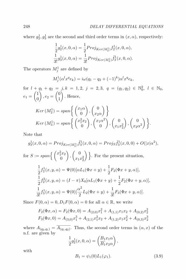
DELAY DIFFERENTIAL EQUATIONS
where g12, g
13 are the second and third order terms in (x, α), respectively:
12g12(x, 0, α) =
12ProjKer(M1
2 )f12 (x, 0, α),
13!
g13(x, 0, α) =
13!
ProjKer(M13 )f
13 (x, 0, α).
The operators M1j are defined by
M1j (αlxqek) = iω(q1 − q2 + (−1)k)αlxqek,
for l + q1 + q2 = j, k = 1, 2, j = 2, 3, q = (q1, q2) ∈ N20, l ∈ N0,
e1 =(
10
), e2 =
(01
). Hence,
Ker (M12 ) = span
(x1α0
),
(0
x2α
)
Ker (M13 ) = span
(x2
1x2
0
),
(x1α
2
0
),
(0
x1x22
),
(0
x2α2
).
Note that
g13(x, 0, α) = ProjKer(M1
3 )f13 (x, 0, α) = ProjS f1
3 (x, 0, 0) + O(|x|α2),
for S := span(
x21x2
0
),
(0
x1x22
). For the present situation,
12f12 (x, y, α) = Ψ(0)[αL1(Φx + y) +
12F2(Φx + y, α)],
12f22 (x, y, α) = (I − π)X0[αL1(Φx + y) +
12F2(Φx + y, α)],
13!
f13 (x, y, α) = Ψ(0)[
α2
2L2(Φx + y) +
13!
F3(Φx + y, α)].
Since F (0, α) = 0, D1F (0, α) = 0 for all α ∈ R, we write
F2(Φx, α) = F2(Φx, 0) = A(2,0)x21 + A(1,1)x1x2 + A(0,2)x
22
F3(Φx, 0) = A(3,0)x31 + A(2,1)x
21x2 + A(1,2)x1x
22 + A(0,3)x
32
where A(q2,q1) = A(q1,q2). Thus, the second order terms in (α, x) of then.f. are given by
12g12(x, 0, α) =
(B1x1αB1x2α
),
withB1 = ψ1(0)L1(ϕ1). (3.9)
248

Normal Forms And Bifurcations For DDE
Now we determine the cubic terms for α = 0. From (2.19), we have
g13(x, 0, 0) = ProjSf1
3 (x, 0, 0)
+32ProjS
[(Dxf1
2 )(x, 0, 0)U12 (x, 0) + (Dyf
12 )(x, 0, 0)U2
2 (x, 0)],
(3.10)where
U12 (x, 0) = U1
2 (x, α)|α=0
= (M12 )−1ProjIm(M1
2 )f12 (x, 0, 0) = (M1
2 )−1f12 (x, 0, 0)
and U22 (x, 0) = U2
2 (x, α)|α=0 is determined by the equation
(M22 U2
2 )(x, 0) = f22 (x, 0, 0).
The elements of the canonical basis for V 32 (C2) are
(x2
1
0
),
(x1x2
0
),
(x2
2
0
),
(x1α0
),
(x2α0
),
(α2
0
)(
0x2
1
),
(0
x1x2
),
(0x2
2
),
(0
x1α
),
(0
x2α
),
(0α2
),
with images under 1iωM1
2 given respectively by(
x21
0
),−(
x1x2
0
),−3
(x2
2
0
),
(00
),−2
(x2α0
),−(
α2
0
)
3(
0x2
1
),
(0
x1x2
),−(
0x2
2
), 2(
0x1α
),
(00
),
(0α2
).
Hence,
U12 (x, 0) =
1iω
(ψ1(0)(A(2,0)x
21 −A(1,1)x1x2 − 1
3A(0,2)x22)
ψ2(0)(13A(2,0)x
21 + A(1,1)x1x2 −A(0,2)x
22)
).
A few computations show that
ProjSf13 (x, 0, 0) =
(ψ1(0)A(2,1)x
21x2
ψ2(0)A(1,2)x1x22
)(3.11)
and
ProjS [(Dxf12 )(x, 0, 0)U1
2 (x, 0)] =(
C1x21x2
C1x1x22
), (3.12)
with
C1 =i
ω
(ψ2
1(0)A(2,0)A(1,1) − |ψ1(0)|2(23|A(2,0)|2 + A2
(1,1)))
.
249

DELAY DIFFERENTIAL EQUATIONS
It remains to determine ProjS [(Dyf12 )(x, 0, 0)U2
2 (x, 0)]. Let H2 : C ×C → C be the bilinear symmetric form such that
F2(u, α) = F2(u, 0) = H2(u, u), u ∈ C
(i.e., F2(u, 0) is the quadratic form associated with H2(u, v)). Then,
(Dyf12 )|y=0,α=0(h) = 2Ψ(0)H2(Φx, h).
Define h = h(x)(θ) by h(x) = U22 (x, 0), and write
h(x) = h20x21 + h11x1x2 + h02x
22,
where h20, h11, h02 ∈ Q1. Using the definition of M22 , AQ1 and π, we
deduce that equation
(M22 h)(x) = f2
2 (x, 0, 0)
is equivalent to
Dxh(x)Bx−AQ1(h(x)) = (I − π)X0F2(Φx, 0),
or, in other words, to
h(x)−Dxh(x)Bx = ΦΨ(0)F2(Φx, 0)
h(x)(0)− L0h(x) = F2(Φx, 0),
where we use the notation h = ddθh. From this system, we deduce
h02 = h20, h11 = h11, and two initial value problems (IVPs),
h20 − 2iωh20 = A(2,0)ΦΨ(0)
h20(0)− L0(h20) = A(2,0)
and h11 = A(1,1)ΦΨ(0)
h11(0)− L0(h11) = A(1,1).
Thus, we obtain
ProjS [(Dyf12 )h](x, 0, 0) =
(C2x
21x2
C2x1x22
), (3.13)
withC2 = 2ψ1(0)[H2(ϕ1, h11) + H2(ϕ2, h20)].
250

Normal Forms And Bifurcations For DDE
Hence, from (3.10)-(3.13) we get
13!
g13(x, 0, 0) =
(B2x
11x2
B2x1x22
),
withB2 =
13!
ψ1(0)A(2,1) +14(C1 + C2). (3.14)
Therefore, the n.f. reads as
x = Bx +(
B1x1αB1x2α
)+(
B2x21x2
B2x1x22
)+ O(|x|α2 + |x|4), (3.15)
with B1, B2 given by (3.9), (3.14). Changing to real coordinates w,where x1 = w1 − iw2, x2 = w1 + iw2, and then to polar coordinates(ρ, ξ), w1 = ρ cos ξ, w2 = ρ sin ξ, Eq. (3.15) becomes
ρ= K1αρ + K2ρ3 + O(α2ρ + |(ρ, α)|4)
ξ= −ω + O(|(ρ, α)|),(3.16)
with the coefficients K1, K2 explicitly given in terms of the original FDEas K1 = ReB1, K2 = ReB2. Recall that the generic Hopf bifurcationcorresponds to the situation K2 = 0, the direction of the bifurcationis determined by the sign of K1K2, and the stability of the nontrivialperiodic orbits is determined by the sign of K2 (see e.g. [30]). Solvingthe two IVPs above, we obtain
h20(θ) = A(2,0)
(e2iωθ
2iω − L0(e2iωθ)− ψ1(0)eiωθ
iω− ψ1(0)e−iωθ
3iω
)
h11(θ) = A(1,1)
(− 1
L0(1)+
1iω
(ψ1(0)eiωθ − ψ1(0)e−iωθ
)).
Theorem 3.3. A Hopf bifurcation occurs from α = 0 on a 2-dimensionallocal centre manifold of the origin. On this manifold, the flow is givenin polar coordinates by Eq. (3.16), with
K1 = Re (ψ1(0)L1(eiωθ)) (3.17)
K2 =13!
Re [ψ1(0)A(2,1)]−A(1,1)
2L0(1)Re [ψ1(0)H2(eiωθ, 1)]
+12Re[ ψ1(0)A(2,0)
2iω − L0(e2iωθ)H2(e−iωθ, e2iωθ)
]. (3.18)
251

DELAY DIFFERENTIAL EQUATIONS
Example 3.4. Consider the well-known Wright equation
u(t) = −au(t− 1)[1 + u(t)], (3.19)
which has been studied by many authors (see [30, 45] and referencestherein). The characteristic equation for the linearization around zero,u(t) = −au(t− 1), is
λ + ae−λ = 0. (3.20)
There is a pair of (simple) imaginary roots ±iω for (3.20) if and only ifa = aN and ω = ωN , where
aN = (−1)NωN , ωN =π
2+ Nπ, N ∈ N0.
With α = a− aN , (3.19) is written as
u(t) = −aNu(t− 1) + αu(t− 1) + F (ut, α), (3.21)
where F (v, α) = −(aN + α)v(0)v(−1). Set Λ = iωN ,−iωN. For ψ(0)as in (3.8), ψ1(0) = 1−iωN
1+ω2N
. Write the Taylor formulas
L(α)v = L0v + L1(α)v, F (v, α) =12F2(v, α) +
13!
F3(v, α),
where L0(v) = −aNv(−1), L1(α)v = −αv(−1) and 12F2(v, α) = −aNv(0)
v(−1), F3(v, α) = −αv(0)v(−1). Applying Theorem 3.3, we obtain then.f. on the center manifold of the origin near a = aN given in polarcoordinates by Eq. (3.16), with
K1 =aN
1 + a2N
,
K2 =ωN
5(1 + a2N )
[(−1)N − 3ωn] < 0, for N ∈ N0.
Thus, a generic Hopf bifurcation for (3.19) occurs from u = 0, a = aN .Since K2 < 0 for all N ∈ N0, the bifurcating periodic orbits are alwaysstable inside the centre manifold. On the other hand, K1 > 0 if Neven, thus K1K2 < 0, and the Hopf bifurcation is supercritical. If N isodd, K1 < 0, thus the Hopf bifurcation is subcritical. E.g., at the firstbifurcating point a = a0 = π/2 (N = 0), we have Λ = iπ/2,−iπ/2,and
K1 =2π
4 + π2> 0, K2 =
π(2− 3π)5(4 + π2)
< 0. (3.22)
252

Normal Forms And Bifurcations For DDE
4. Normal Forms for FDEs in Hilbert SpacesIn the following, X is a real or complex Hilbert space with inner
product < ·, · > and C = C([−r, 0]; X) (r > 0) is the Banach spaceof continuous maps from [−r, 0] to X with the sup norm. In orderto simplify the notation, fix R as the scalar field. Write ut ∈ C forut(θ) = u(t + θ),−r ≤ θ ≤ 0, and consider FDEs in X given in abstractform as
u(t) = AT u(t) + L(ut) + F (ut) (t ≥ 0), (4.1)
where AT : D(AT ) ⊂ X → X is a linear operator, L ∈ L(C; X), i.e.,L : C → X is a bounded linear operator, and F : C → X is a Ck
function (k ≥ 2) such that F (0) = 0, DF (0) = 0.We are particularly interested in equations (4.1), since they include
reaction-diffusion (RD) equations with delays appearing in the reactionterms. Equations involving both time delays and spatial diffusion havebeen increasingly used in population dynamics, neural networks, diseasemodelling, and other fields.
A typical example of a RD-equation with delays is the so-calledlogistic equation with delays and spatial diffusion. In the framework ofODEs, consider the logistic equation x = ax(1 − bx), where a is thegrowth rate of the population and K = 1/b the “carrying capacity”.Taking into account the maturation period r > 0 of the population, themodel becomes
x(t) = ax(t)[1− bx(t− r)],
known as the Hutchinson equation. Translating the positive equilibrium1/b to the origin and effecting a scaling, y(t) = bx(t) − 1, we get theWright equation (conf. Example 3.4)
y(t) = −ay(t− r)[1 + y(t)].
Considering also a spatial variable x ∈ [0, 1], and diffusion terms, weobtain the model
∂v
∂t(t, x) = d
∂2v
∂x2− av(t− r, x)[1 + v(t, x)], t > 0, x ∈ (0, 1),
to which boundary conditions, such as Neumann or Dirichlet conditions,should be added. This RD-equation is often used as a model in popula-tion dynamics, where v stands for the density of the population spreadover the interval [0, 1], d is the diffusion rate that measures the internalmigration of the population, and a, b, r have the same meaning as before.
253

DELAY DIFFERENTIAL EQUATIONS
4.1 Linear FDEs
For the linearized equation about the equilibrium zero
u(t) = AT u(t) + L(ut), (4.2)
we assume in this section the following hypotheses (see [73, 77, 101, 104]):
(H1) AT generates a C0-semigroup of linear operators T (t)t≥0 on X;
(H2) T (t) is a compact operator for t > 0;
(H3) the eigenfunctions βk∞k=1 of AT , with corresponding eigenvaluesµk∞k=1, form an orthonormal basis for X;
(H4) the subspaces Bk of C, Bk := ϕβk |ϕ ∈ C([−r, 0]; R), satisfyL(Bk) ⊂ spanβk, k ∈ N.
For a straightforward generalization of these assumptions to equa-tions (4.2) in Banach spaces see [101, Chapter 3]. For a weaker versionof (H4) see [36].
Hypothesis (H4) roughly requires that the operator L does not mixthe spatial variations described by eigenvectors βk of AT . This conditionis very restrictive in terms of applications, since it almost imposes thatL is a scalar multiplication. In Section 5 of the present text, normalforms are developed for FDEs in Banach spaces without imposing (H3)-(H4). Nevertheless, the situation where (H1)-(H4) hold will be studiedseparately in this section since it provides a strong result: eventuallyunder additional conditions, for (4.1) it is possible to associate an FDEin R
n, whose n.f. on invariant manifolds coincide with n.f. on invariantmanifolds for (4.1), up to some order. This allows us to apply to (4.1)the n.f. method for FDEs in R
n described in Section 2 without furthercomputations.
As for retarded FDEs in Rn, we start by looking for solutions of the
linear equation (4.2) of the exponential type,
u(t) = eλty, y ∈ D(AT ).
Clearly u(t) as above is a non-trivial solution of (4.2) if and only if λ, ysatisfy the characteristic equation
∆(λ)y = 0, λ ∈ C, y ∈ D(AT ) \ 0, (4.3)
where the characteristic operator ∆(λ) is defined by
∆(λ) : D(AT ) ⊂ X → X, ∆(λ)y = λy −AT y − L(eλ·y).
254

Normal Forms And Bifurcations For DDE
Let A be the infinitesimal generator associated with the semiflowof the linearized equation (4.2). It is well-known ([73, 77, 92, 101, 104])that its eigenvalues are exactly the roots of the characteristic equation(4.3), that the spectrum of A is reduced to the point spectrum and that,for each α ∈ R, the set σ(A) ∩ λ ∈ C : Reλ ≥ α is finite.
Since (H4) states that L does not mix the modes of eigenvaluesof AT , and from (H3) X can be decomposed by βk∞k=1, we deducethat equation ∆(λ)y = 0 is equivalent to the sequence of characteristicequations
λ− µk − Lk(eλ·) = 0 (k ∈ N), (4.4k)
where Lk : C([−r, 0]; R) → R are defined by Lk(ψ)βk = L(ψβk), fork ∈ N.
Again, for the sake of applications, we fix Λ = λ ∈ σ(A) : Reλ =0 = ∅, and let P be the centre space for (4.2). Since Λ is a finite set,there exists N ∈ N, such that Λ = λ ∈ C : λ is a solution of (4.4k)with Re λ = 0, for some k ∈ 1, . . . , N.
We describe briefly an adjoint theory for FDEs (4.2) as in [73, 77],assuming the above hypotheses. The main idea is to relate the eigenval-ues of the infinitesimal generator A (in this case, only the elements of Λ)with the eigenvalues of certain scalar FDEs. On Bk, the linear equationu(t) = AT u(t) + L(ut) is equivalent to the FDE on R
z(t) = µkz(t) + Lkzt , (4.5k)
with characteristic equation given by (4.4k), k ∈ N. With this identifi-cation, the standard adjoint theory for retarded FDEs can be used todecompose C, in the following way. For 1 ≤ k ≤ N , define (·, ·)k asthe adjoint bilinear form on C([0, r]; R∗)×C([−r, 0]; R) associated with(4.5k), and decompose C([−r, 0]; R) by Λk := λ ∈ C : λ satisfies (4.4k)and Re λ = 0 as in Section 2.1 (see [58]):
C([−r, 0]; R) = Pk ⊕Qk , Pk = spanΦk , P ∗k = spanΨk ,
(Ψk, Φk)k = I , dimPk = dimP ∗k := mk , Φk = ΦkBk ,
where Pk is the centre space for (4.5k) and Bk is an mk ×mk constantmatrix. For each k ∈ N, the projection Pk ⊕Qk → Pk, u → Φk(Ψk, u)k
induces a projection
C → Pkβk, ϕ → Φk(Ψk, < ϕ(·), βk >)kβk.
We use the above decompositions to decompose C by Λ:
C = P ⊕Q , P = Im π , Q = Kerπ,
255

DELAY DIFFERENTIAL EQUATIONS
where dim P =∑N
k=1 mk := M and π : C −→ P is the canonicalprojection defined by
πφ =N∑
k=1
Φk(Ψk, < φ(·), βk >)kβk .
4.2 Normal forms
As for retarded FDEs in Rn, we first enlarge the phase space so
that (4.1) can be written as an abstract ODE, along the lines of Section2. Denote by X0 the function defined by X0(0) = I, X0(θ) = 0 , −r ≤θ < 0, where I is the identity operator on X, and let
BC ≡ C ×X = φ + X0α : φ ∈ C,α ∈ X.
In BC, (4.1) reads as an abstract ODE,
d
dtv = Av + X0F (v), (4.6)
where A is the extension of the infinitesimal generator A defined by
A : C10 ⊂ BC −→ BC
D(A) = C10 := φ ∈ C : φ ∈ C, φ(0) ∈ D(AT )
Aφ = φ + X0[L(φ) + AT φ(0)− φ(0)].
We further consider the extension of the projection π : C → P to BC,still denoted by π, by defining
π(X0α) =N∑
k=1
ΦkΨk(0) < α, βk > βk, α ∈ X.
By using π, the enlarged space BC is decomposed by Λ as
BC = P ⊕Kerπ,
with Q ⊂ Ker π and P ⊂ C10 . One can prove that π is continuous and
commutes with A in C10 . For v ∈ C1
0 , using the above decomposition,we write
v(t) =N∑
k=1
Φkxk(t) + y(t), with xk(t) ∈ R, 1 ≤ k ≤ N, y ∈ C10 ∩ Ker π := Q1.
256
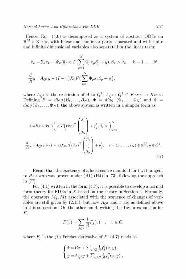
Normal Forms And Bifurcations For DDE
Hence, Eq. (4.6) is decomposed as a system of abstract ODEs onR
M × Ker π, with linear and nonlinear parts separated and with finiteand infinite dimensional variables also separated in the linear term:
xk =Bkxk + Ψk(0) < F (N∑
p=1
Φpxpβp + y), βk > βk, k = 1, . . . , N,
d
dty =AQ1y + (I − π)X0F
( N∑p=1
Φpxpβp + y),
where AQ1 is the restriction of A to Q1, AQ1 : Q1 ⊂ Ker π → Ker π.Defining B = diag (B1, . . . , BN ), Φ = diag (Φ1, . . . ,ΦN ) and Ψ =diag (Ψ1, . . . ,ΨN ), the above system is written in a simpler form as
x =Bx + Ψ(0)
(< F
((Φx)
β1
...
βN
+ y
), βk >
)N
k=1
d
dty =AQ1y + (I − π)X0F
((Φx)
β1
...
βN
+ y
), x = (x1, . . . , xN ) ∈ R
M , y ∈ Q1.
(4.7)
Recall that the existence of a local centre manifold for (4.1) tangentto P at zero was proven under (H1)-(H4) in [73], following the approachin [77].
For (4.1) written in the form (4.7), it is possible to develop a normalform theory for FDEs in X based on the theory in Section 2. Formally,the operators M1
j , M2j associated with the sequence of changes of vari-
ables are still given by (2.13), but now AQ1 and π are as defined abovein this subsection. On the other hand, writing the Taylor expansion forF ,
F (v) =∑j≥2
1j!
Fj(v) , v ∈ C,
where Fj is the jth Frechet derivative of F , (4.7) reads as
x =Bx +
∑j≥2
1j!f
1j (x, y)
y =AQ1y +∑
j≥21j!f
2j (x, y) ,
257

DELAY DIFFERENTIAL EQUATIONS
with the terms f ij(x, y), i = 1, 2, j ≥ 2, given here by
f1j (x, y) = Ψ(0)
(< Fj
((Φx)
β1...
βN
+ y
), βk >
)N
k=1
f2j (x, y) = (I − π)X0Fj
((Φx)
β1...
βN
+ y
), x ∈ R
M , y ∈ Q1.
The main results in Section 2 are still valid in this setting. Details andexamples of applications can be found in [37].
4.3 The associated FDE on RN
.If we compare Eq. (4.7) with Eq. (2.6), it is natural to associate
an FDE in RN with the original FDE (4.1). In fact, formally we relate
(4.7) with the DDE in RN
x = Bx + Ψ(0)G(Φx + y)y = AQ1y + (I − π)X0G(Φx + y),
(4.8)
for the nonlinearity G : CN := C([−r, 0]; RN ) → RN defined by
G(φ) =(
< Fj
(φ
β1...
βN
), βk >
)N
k=1
. (4.9)
However, the operators A and π are defined differently in (4.7) and (4.8).On the other hand, in order to derive the linear terms in (4.8) from theprocedure in Section 2.2, the linearization of the original FDE in R
N
(2.1) should have the form u(t) = R(ut), with R ∈ L(CN ; RN ) definedby
R(φ) = (µkφk(0) + Lk(φk))Nk=1, (4.10)
for φ = (φ1, . . . , φN ) ∈ C([−r, 0]; RN ) (cf. (4.5k), k = 1, . . . , N).
Definition 4.1. The following FDE in CN := C([−r, 0]; RN ) is said tobe the FDE in R
N associated with Eq. (4.1) by Λ at zero:
x(t) = R(xt) + G(xt), (4.11)
where x(t) =(xk(t)
)Nk=1
, xt =(xt,k
)Nk=1
, and G, R are defined by (4.9),(4.10).
258

Normal Forms And Bifurcations For DDE
The relevance of this associated FDE in RN is summarized in the
next theorem.Theorem 4.2. [37] Consider Eq. (4.1), and assume (H1)-(H4).
(i) if F is of class C2, then, for a suitable change of variables, then.f. on the centre manifold for both (4.1) and (4.11) is the same, up tosecond order terms;
(ii) if F is of class C3, F (v) =12!
F2(v) +13!
F3(v) + o(|v|3), and
Proj spanβ1,...,βNDF2(u)(φβj) = 0 , for j ≥ N+1, u ∈ P, φ ∈ C([−r, 0]; R), (H5)
then, for a suitable change of variables, the n.f. on the centre manifoldfor both (4.1) and (4.11) are the same, up to third order terms.
Note that assumption (H5) can also be written as
< DF2(u)(φβj), βp >= 0 , for 1 ≤ p ≤ N, j > N and all u ∈ P, φ ∈ C([−r, 0]; R).
The proof of this theorem is based on the possibility of identifyingthe operators M1
j , M2j of the n.f. algorithm for (4.1) with the corre-
sponding operators appearing in the computation of n.f. relative to Λfor (4.11). The above result is not completely surprising. In fact, notethat (H4) can be interpreted as nonresonance conditions of first order,in the sense that it imposes nonresonances inside the linear part of theequation, between L and the operator AT . Now recall that second or-der terms of n.f. are computed by looking at second order terms in theequation for x ∈ R
N . The cubic terms of n.f. are obtained by using notonly second and third order terms in the equation for x ∈ R
N , but alsosecond order terms in the equation for y ∈ Kerπ. Therefore, it is notsurprising to expect the quadratic terms in the n.f. for the flow on thecentre manifold for both equations (4.1) and (4.11) to be the same. Onthe other hand, it is natural to expect that additional nonresonance con-ditions of second order should be imposed, in order to derive the sameresult for cubic terms. The role of (H5) is to impose such nonresonanceconditions, between the second order terms of F and the eigenspaces forAT . Of course, we could derive other nonresonance conditions betweenthe j-order terms (j ≤ k − 1) of F and the eigenspaces for AT , in orderto conclude that the n.f. on the centre manifold for both (4.1) and (4.11)are the same up to k order terms. In the present framework, Theorem4.2 is particularly relevant, since it enables us to reduce the computationof n.f. for FDEs in Hilbert spaces X to the computation of n.f. for FDEsin finite dimensional spaces. Moreover, even if (H5) fails, one can prove
259

DELAY DIFFERENTIAL EQUATIONS
[37] that the associated FDE by Λ (4.11) still carries much informationthat can be used when computing n.f. for (4.1).
4.4 Applications to bifurcation problems
Population dynamics models involving memory and diffusion in onespatial variable are often given by equations of the form
∂u(t, x)∂t
= d∂2u(t, x)
∂x2+ a(x)u(t, x) + b(x)u(t− r, x)
+ c0(x)u(t, x)u(t− r, x), t > 0, x ∈ (1, 2),
with either Neumann or Dirichlet boundary conditions on [1, 2] ⊂ R,and initial condition
u0 = ϕ ∈ C = C([−r, 0]; X).
For the choice e.g. X = L2[1, 2] , the problem is not well-posed,since L2[1, 2] is not a Banach algebra. However, the question of exis-tence of solutions will not be addressed here, since that is not the aimof the n.f. theory. In order to guarantee existence of solutions, thereare several approaches. One can restrict the state space to an appro-priate space of functions invariant under products, e.g. X = C[1, 2]or X = W 2,2[1, 2] [73, 77, 101]. Another possibility is to considera fractional power (AT )β of AT (0 < β < 1), and take as the Ba-nach state space the fractional power space Xβ = D(Aβ), with norm‖v‖β = ‖(AT )βv‖; and Cβ = C([−1, 0]; Xβ) as the phase space. Thistheory is well established since the work of Henry [63]. See also [[46, 54, 93, 94]. Another procedure is to consider X = L2[1, 2], and re-strict the space of initial conditions that are chosen in a natural “initial-history” space [85, 86].
As an application, we shall consider the Wright equation with dif-fusion. For an application of the n.f. theory to a 2-dimensional RD-equation with two delays, see [40].
Example 4.3. Consider the Wright equation with diffusion and Neu-mann conditions ([37, 73, 77, 104]):
∂u(t, x)∂t
= d∂2u(t, x)
∂x2− au(t− 1, x)[1 + u(t, x)], t > 0, x ∈ (0, π)
∂u(t, 0)∂x
=∂u(t, π)
∂x= 0 , t ≥ 0,
(4.12)
260

Normal Forms And Bifurcations For DDE
where d > 0, a > 0. Let X = W 2,2(0, π) and C = C([−1, 0]; X). Inabstract form in C, (4.12) is given by
d
dtu(t) = d∆u(t) + L(a)(ut) + f(ut, a) (4.13)
where ∆ = ∂2
∂x2 , D(∆) = v ∈ W 2,2(0, π) : dvdx = 0 at x = 0, π and
L(a)(v) = −av(−1), f(v, a) = −av(0)v(−1).The eigenvalues of AT = d∆ are µk = −dk2, k ≥ 0, with corre-
sponding normalized eigenfunctions βk(x) = cos(kx)‖ cos(kx)‖2,2
. One can easilycheck that (H1)-(H4) hold. For the linearization of (4.13) about the equi-librium u = 0, the characteristic equation is equivalent to the sequenceof characteristic equations
λ + ae−λ + dk2 = 0 , (k = 0, 1, . . . ). (4.14k)
Yoshida [104] showed that for a < π/2, all roots have negative realparts, thus the zero solution is asymptotically stable; for a = π/2 andk = 0, there exists a unique pair of characteristic values on the imaginaryaxis, ±iπ/2, that are simple roots, and that all the other characteristicvalues of (4.14k), k ∈ N0, have negative real parts. At the critical pointa = π/2, rescale the parameter by setting a = π/2 + α. Since theHopf condition holds [104], i.e., there is a pair of eigenvalues crossingtransversely the imaginary axis at α = 0, a Hopf bifurcation occurs ona 2-dimensional centre manifold.
Let Λ = iπ/2,−iπ/2. With the above notations (except thathere k ∈ N0 instead of k ∈ N), N = 0, µ0 = 0, β0 = 1√
π. Since
L(ψβ0) = −π2 ψ(−1)β0, the operator L0 : C([−1, 0]; R) → R in (4.40),
corresponding to the eigenvalue µ0 = 0, is defined by
L0(ψ) = −π
2ψ(−1).
The associated FDE (on R) by Λ at the equilibrium point u = 0, α = 0is
x(t) = L0(xt)+ < F(xtβ0, α
), β0 >, (4.15)
where F (v, α) = −αv(−1)− (π2 + α)v(0)v(−1). We have
< F (xtβ0, α), β0 > = − < αx(t − 1)1√π
+ (π
2+ α)x(t)
1√π
x(t − 1)1√π
,1√π
>
= −x(t − 1)[α + (π
2+ α)
1√π
x(t)]
.
Thus, (4.15) becomes
x(t) = −(π
2+ α)x(t− 1)[1 +
1√π
x(t)], (4.16)
261

DELAY DIFFERENTIAL EQUATIONS
i.e., (4.16) is the Wright equation (3.19) for the scaling x → 1√πx.
We prove now that hypothesis (H5) is satisfied. He have
F2(v, α) = −αv(−1)− π
2v(0)v(−1), v ∈ C,α ∈ R.
For u ∈ P , write u = Φ0cβ0, where c ∈ C2 and Φ0 is a basis for the centre
space P0 for the linear FDE in R (4.50), i.e., x(t) = L0(xt). Then,
12
< D1F2(u, α)(ψβk), β0 >
= −α < ψ(−1)βk, β0 > −π
2<(u(0)ψ(−1) + u(−1)ψ(0)
)βk, β0 >
= −[αψ(−1) +
√π
2(Φ0(0)cψ(−1) + Ψ0(−1)cψ(0)
)]< βk, β0 >= 0,
for all k ≥ 1, c ∈ C2, ψ ∈ C([−1, 0]; R). This implies (H5).
For (3.19), the n.f. on the centre manifold is given in polar coordi-nates (ρ, ξ) by (3.16), where K1, K2 are given by (3.22). Effecting thescaling x → 1√
πx, from Theorem 4.2 we deduce the n.f. on the centre
manifold for (4.12) without further computations:
ρ =K1αρ +1π
K2ρ3 + O
(α2ρ + |(ρ, α)|4
)
ξ =− π
2+ O
(|(ρ, α)|
),
with K1, K2 as in (3.22). Thus, a generic supercritical Hopf bifurcationoccurs on the centre manifold for (4.12), with stable nontrivial bifurcat-ing periodic solutions.
5. Normal Forms for FDEs in General BanachSpaces
Consider again a semilinear FDE (4.1) in the phase space C :=C([−r, 0]; X),
u(t) = AT u(t) + L(ut) + F (ut), (5.1)
where now X is a general Banach space, AT : D(AT ) ⊂ X → X is linear,and F : C → X is Ck (k ≥ 2) with F (0) = 0, DF (0) = 0.
Before developing a normal form theory on an invariant manifold forFDEs (5.1), it is necessary to establish two necessary technical tools: aformal adjoint theory for linear equations, and the existence and smooth-ness of centre manifolds for nonlinearly perturbed equations (5.1) ([43]).
262

Normal Forms And Bifurcations For DDE
5.1 Adjoint theoryConsider a linear FDE in C of the form
u(t) = AT u(t) + L(ut), (5.2)
where AT , L are as in (5.1). In this section, we shall assume only thefollowing hypotheses:
(H1) AT generates a C0 semigroup of linear operators T (t)t≥0 on X;
(H2) T (t) is a compact operator for t > 0;
(H3) there exists a function η : [−r, 0]→ L(X, X) of bounded variationsuch that
L(ϕ) =∫ 0
−rdη(θ)ϕ(θ), ϕ ∈ C.
Under (H1)-(H3), a complete formal adjoint theory was developedin [43], and will be presented here, following some ideas in [16] and [92].The adjoint theory for abstract FDEs was initiated in [92]. However, thetheory in [92] was quite incomplete and more hypotheses were assumed.On the other hand, Arino and Sanchez [16] developed a complete formaladjoint theory for equations u(t) = L(ut). From the point of view ofthe applications we have in mind, equations in the form (5.1) are moreinteresting, since they include RD-equations with delays. In [16], theauthors worked only with characteristic values that are not in the es-sential spectrum in order to obtain Fredholm operators, whereas in oursetting we will be dealing with compact operators. Note that, contraryto the situation studied in Section 4, we are not imposing any conditionswhich relate L with the eigenvalues for AT .
Consider the characteristic equation (4.3) for (5.2),
∆(λ)x = 0, x ∈ D(AT ) \ 0 (5.3)
where the characteristic operator ∆(λ) : D(AT ) ⊂ X → X is defined by
∆(λ)x = AT x + L(eλ·x)− λx.
We start by recalling the results in [92]. Consider the C0-semigroupof linear operators U(t)t≥0, defined by the mild solutions of (5.2) withinitial condition ϕ ∈ C, U(t) : C → C,U(t)ϕ = ut(ϕ), and its infinitesi-mal generator A,
Aϕ = ϕ, D(A) = ϕ ∈ C : ϕ ∈ C,ϕ(0) ∈ D(AT ), ϕ(0) = AT ϕ(0) + L(ϕ).
263

DELAY DIFFERENTIAL EQUATIONS
Travis and Webb [92] proved that U(t) is a compact operator for eacht > r and σ(A) = σP (A). From general results on C0-semigroups andcompact operators (see e.g. [84]), it follows that, for λ ∈ σ(A),
C = Ker [(A− λI)m]⊕ Im [(A− λI)m], (5.4)
where Im [(A − λI)m] is a closed subspace of C and Ker [(A − λI)m]is the generalized eigenspace for A associated with λ, denoted as usualby Mλ(A), with Mλ(A) finite dimensional. In particular, the ascentand descent of A − λI are both equal to m, where m is the order ofλ as a pole of the resolvent R(λ; A) [90]. Our purpose now is to writeIm [(A − λI)m] in terms of a (formal) adjoint theory, in the sense thata Fredholm alternative result should be established.
As seen in Section 4.1, λ is a characteristic value if and only λ isan eigenvalue of A, and, in this case, there is x ∈ D(AT ) \ 0 such thatu(t) = eλtx is a solution of (5.2). Thus,
Ker (A− λI) = eλ·x : x ∈ Ker ∆(λ). (5.5)
We use the formal duality << ·, · >> in C∗ × C introduced in [92]as the bilinear form
<< α, ϕ >>=< α(0), ϕ(0) > −∫ 0
−r
∫ θ
0< α(ξ − θ), dη(θ)ϕ(ξ) > dξ
where C∗ := C([0, r]; X∗), X∗ is the dual of X, and < ·, · > is the usualduality in X∗ ×X. Define the formal adjoint equation to (5.2) as
α(t) = −A∗T α(t)− L∗(αt), t ≤ 0, (5.6)
where αt ∈ C∗, αt(s) = α(t+ s) for s ∈ [0, r], A∗T is the adjoint operator
for AT , L∗ : C∗ → X∗ is given by L∗(α) =∫ 0−r dη∗(θ)α(−θ), and η∗(θ)
is the adjoint for η(θ), η∗ : [−r, 0] → L(X∗, X∗). Let A∗ be the infini-tesimal generator associated with the flow for (5.6). The operator A∗ iscalled the formal adjoint of A, since
<< A∗α, ϕ >>=<< α, Aϕ >> , for α ∈ D(A∗), ϕ ∈ D(A).
Inspired by the work of Hale [58, Chapter 7] and [16], we nowintroduce some auxiliary operators, that will be used first of all to get anexplicit characterization of the null spaces and ranges for the operators(A − λI)m and (A∗ − λI)m. Let λ ∈ C, j ∈ N0, m ∈ N, and define theoperators
Ljλ : X → X, Lj
λ(x) = L(θj
j!eλθx
),
264

Normal Forms And Bifurcations For DDE
L(m)λ : Xm → Xm, L(m)
λ =
∆(λ) L1λ − I L2
λ . . . Lm−1λ
0 ∆(λ) L1λ − I . . . Lm−2
λ...
.... . . . . .
...0 0 . . . ∆(λ) L1
λ − I0 0 . . . 0 ∆(λ)
and
R(m)λ : C → Xm, R(m)
λ (ψ) =
−L( ∫ θ
0 eλ(θ−ξ) (θ−ξ)m−1
(m−1)! ψ(ξ)dξ)
...−L( ∫ θ
0 eλ(θ−ξ)(θ − ξ)ψ(ξ)dξ)
ψ(0)− L( ∫ θ
0 eλ(θ−ξ)ψ(ξ)dξ).
Theorem 5.1. Let λ ∈ C, m ∈ N. Then:
(i) Ker [(A−λI)m] =∑m−1
j=0θj
j! eλθuj , θ ∈ [−r, 0], with
u0...
um−1
∈
Ker (L(m)λ )
;
(ii) ψ ∈ Im [(A− λI)m] iff R(m)λ (ψ) ∈ Im (L(m)
λ );
(iii) Ker [(A∗ − λI)m] =∑m−1
j=0(−s)j
j! e−λsx∗m−j−1, s ∈ [0, r], with
x∗0
. . .x∗
m−1
∈ Ker ((L(m)
λ )∗)
.
The proof of this theorem follows from direct computations, so it isomitted. See [16, 58] for similar proofs.
We now establish some preliminary lemmas.Lemma 5.2. The characteristic operator ∆(λ) generates a compactC0-semigroup of linear operators on X. Moreover, λ ∈ σ(A) if and onlyif 0 ∈ σ(∆(λ)).
Proof. From (5.4), clearly λ ∈ ρ(A) if and only if 0 is not an eigenvalueof ∆(λ). On the other hand, ∆(λ) is the sum of AT , which generatesa compact C0-semigroup, with the bounded linear operator L0
λ − λI.Hence, ∆(λ) generates a compact semigroup of linear operators on X[84, p. 79]. This also implies that 0 ∈ ρ(∆(λ)) iff 0 ∈ σP (∆(λ)). Henceλ ∈ ρ(A) iff 0 ∈ ρ(∆(λ)).Lemma 5.3. Let λ ∈ C and m ∈ N. Then:
(i) if µ ∈ ρ(∆(λ)), then µ ∈ ρ(L(m)λ ) and (L(m)
λ − µI)−1 is a compactoperator;
265

DELAY DIFFERENTIAL EQUATIONS
(ii) Im (L(m)λ ) is a closed subspace of Xm.
Proof. Let µ ∈ ρ(∆(λ)). For m = 1, we have L(1)λ = ∆(λ), and from
Lemma 5.2 we conclude that this operator generates a compact C0-semigroup. Thus, its resolvent R(∆(λ); µ) = [∆(λ)−µI]−1 is a compactoperator. The rest of the proof of (i) follows by induction. For the proofof (ii), we use (i) and general spectral properties of compact operators.See [43] for details.Lemma 5.4. Let λ ∈ C, m ∈ N. Then,
dimKer (L(m)λ ) = dimKer ((L(m)
λ )∗) (5.7)
Proof. Let λ ∈ σ(A). From Lemma 5.2, 0 ∈ σ(∆(λ)). Fix anyµ ∈ ρ(∆(λ)). From Lemma 5.3 we deduce that µ ∈ ρ(L(m)
λ ). One canprove that
Ker (L(m)λ ) = Ker ((L(m)
λ − µI)−1 +I
µ),
Ker ((L(m)λ )∗) = Ker ([(L(m)
λ )∗ − µI]−1 +I
µ).
(5.8)
where [(L(m)λ )∗ − µI]−1 = [(L(m)
λ − µI)−1]∗. Also from Lemma 5.3, wehave that (L(m)
λ − µI)−1 is a compact operator, and from Schauder’stheorem we conclude that its adjoint [(L(m)
λ − µI)−1]∗ is also a compactoperator. In particular,
dim Ker ((L(m)λ − µI)−1 +
I
µ) = dimKer ([(L(m)
λ − µI)−1]∗ +I
µ). (5.9)
From (5.8) and (5.9), we obtain (5.7).
As an immediate consequence of Theorem 5.1 and Lemma 5.4, wecan now state the following:Theorem 5.5. Let λ ∈ C, m ∈ N. Then,
dimKer [(A− λI)m] = dimKer [(A∗ − λI)m].
In particular, σP (A) = σP (A∗), and for λ ∈ σP (A),
dimMλ(A) = dimMλ(A∗),
and the ascents of both operators A− λI and A∗ − λI are equal. Thatis, if Mλ(A) = Ker [(A− λI)m], then Mλ(A∗) = Ker [(A∗ − λI)m].
We are now in the position to state a “Fredholm alternative” result.
266

Normal Forms And Bifurcations For DDE
Theorem 5.6. Let λ ∈ σ(A), m ∈ N. Then ψ ∈ Im [(A− λI)m] if andonly if
<< α, ψ >>= 0 for all α ∈ Ker [(A∗ − λI)m].
Proof. From Lemma 5.3, the ranges of L(m)λ are closed subspaces,
hence they coincide with the annihilator of the adjoint operator (L(m)λ )∗,
Im (L(m)λ ) = Ker ((L(m)
λ )∗)⊥.
From Theorem 5.1, ψ ∈ Im [(A − λI)m] iff R(m)λ (ψ) ∈ Im (L(m)
λ ), thusψ ∈ Im [(A− λI)m] iff
< Y ∗,R(m)λ (ψ) >= 0 for all Y ∗ ∈ Ker ((L(m)
λ )∗).
By using the formal duality, for Y ∗ = (y∗0, . . . , y∗m−1)
T ∈ (X∗)m oneproves that
< Y ∗,R(m)λ (ψ) >
= −m−1∑j=0
< y∗j , L(∫ θ
0eλ(θ−ξ) (θ − ξ)m−j−1
(m− j − 1)!ψ(ξ)dξ
)> + < y∗m−1, ψ(0) >
=m−1∑j=0
<< e−λs (−s)m−j−1
(m− j − 1)!y∗j , ψ >> .
Using again Theorem 5.1, we deduce that α ∈ Ker [(A∗ − λI)m] if andonly if
α =m−1∑j=0
e−λs (−s)m−j−1
(m− j − 1)!y∗j ,
with Y ∗ = (y∗0, . . . , y∗m−1)
T ∈ Ker ((L(m)λ )∗). The above arguments im-
ply that ψ ∈ Ker [(A − λI)m] if and only if << α, ψ >>= 0 for allα ∈ Ker [(A∗ − λI)m].
From the Fredholm alternative result in Theorem 5.6, we denoteIm [(A − λI)m] = Ker [(A∗ − λI)m]⊥, where the orthogonality “⊥” isrelative to the formal duality << ·, · >>. For the particular case of mbeing the ascent of A − λI, i.e., Ker [(A − λI)m] = Mλ(A), from (5.4)we obtain the decomposition of the phase space C by λ ∈ σ(A) given as
C = Pλ ⊕Qλ, (5.10)
where Pλ :=Mλ(A) and Qλ :=[Mλ(A∗)
]⊥. It is straightforward to gen-
eralize this decomposition to a nonempty finite set Λ = λ1, . . . , λs ⊂
267

DELAY DIFFERENTIAL EQUATIONS
σ(A). For applications to bifurcation problems, we will as usual fixΛ = λ ∈ σ(A) : Reλ = 0. The decompositions (5.10), λ ∈ Λ, yield adecomposition of C by Λ as
C = P ⊕Q, (5.11)
where
P = Mλ1(A)⊕ · · · ⊕Mλs(A)
Q =[P ∗]⊥ = ϕ ∈ C : << α, ϕ >>= 0, for all ∈ P ∗
andP ∗ =Mλ1(A
∗)⊕ · · · ⊕Mλs(A∗).
Clearly P, Q are invariant subspaces under A and (5.2). One also provesthat for any m, r ∈ N, if λ, µ ∈ σ(A) and λ = µ, then << α, ϕ >>= 0for all α ∈ Ker [(A∗ − λI)m] and ϕ ∈ Ker [(A − µI)r]. By using theFredholm alternative result, it is therefore possible to choose normalizedbases Φ, Ψ for P, P ∗,
Φ = (Φλ1 , . . . ,Φλs), P = span Φ
Ψ =
Ψλ1
. . .Ψλs
, P ∗ = span ΨΛ
where p = dimP = dimP ∗, such that << Ψ, Φ >>= Ip.
5.2 Normal forms on centre manifoldsConsider now Eq. (5.1), which can be interpreted as a perturbation
of (5.2), and assume that Λ = λ ∈ σ(A) : Reλ = 0 is nonempty. Withthe above notations, P is the centre space for (5.2), and p = dimP .Assuming F is a C1 function, in [69], the existence of a C1-smooth p-dimensional centre manifold for (5.2) tangent to P at zero was proven.The following centre manifold theorem states that actually the centremanifold is Ck-smooth.Theorem 5.7. [43, 69] For (5.1) with F a Ck (k ≥ 1) function, there isa centre manifold Wc = ϕ ∈ C : ϕ = Φx + h(x), x ∈ V , where V is aneighbourhood of 0 ∈ R
p, and h : V → Q is a Ck-smooth function suchthat h(0) = 0, Dh(0) = 0.
By using the decomposition (5.11), on Wc the flow is given by theODE
x = Bx+ < Ψ(0), F (Φx + h(x)) >, x ∈ V,
where Φ, Ψ are normalized dual bases for bases of P, P ∗, and B is thep× p matrix such that Φ = ΦB,−Ψ = BΨ.
268

Normal Forms And Bifurcations For DDE
Let Eq. (5.1) be written as the abstract ODE (4.6) in the enlargedphase space BC introduced in Section 4. Recall the definition of theextension A of the infinitesimal generator A. Define now an extensionof the canonical projection C = P ⊕Q→ P ,
π : BC → P, π(ϕ + X0α) = Φ(
<< Ψ, ϕ >> + < Ψ(0), α >).
Again, π commutes with A on C10 = D(A). Hence BC is decomposed
by Λ asBC = P ⊕Ker π. (5.12)
For v(t) ∈ C10 decomposed according to (5.12), v(t) = Φx(t) + y(t) with
x(t) =<< Ψ, v(t) >>∈ Rp, y(t) = (I−π)v(t) ∈ Ker π∩C1
0 = Q∩C10 :=
Q1, Eq. (4.6) is equivalent to the system
x = Bx+ < Ψ(0), F (Φx + y) >
y = AQ1y + (I − π)X0F (Φx + y)(5.13)
where AQ1 = A|Q1 is as in Section 4.The algorithm of n.f. now follows along lines similar to the ones in
Section 2. Writing the formal Taylor expansion of F ,
F (v) =∑j≥2
1j!
Fj(v), v ∈ C,
system (5.13) becomes
x = Bx +∑
j≥21j!f
1j (x, y)
y = AQ1y +∑
j≥21j!f
2j (x, y)
where now the terms of order j are given by
f1j =< Ψ(0), F (Φx + y) >, f2
j = (I − π)X0F (Φx + y). (5.14)
At each step j ≥ 2, a change of variables of the form
(x, y) = (x, y) +1j!
(U1j (x), U2
j (x)),
(U1j ∈ V p
j (Rp), U2j ∈ V p
j (Ker π)) is performed, so that all the non-resonant terms of degree j vanish in the transformed equation. Formally,the operators appearing in the n.f. process are still given by (2.13); how-ever the operators π and AQ1 are as defined in this subsection. Of course,for these operators, results similar to the ones proven for the case of n.f.for FDEs in R
n must be established. See [39] for complete proofs.
269
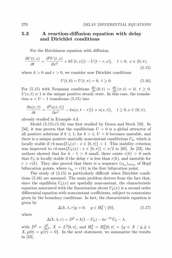
DELAY DIFFERENTIAL EQUATIONS
5.3 A reaction-diffusion equation with delayand Dirichlet conditions
For the Hutchinson equation with diffusion,
∂U(t, x)∂t
=∂2U(t, x)
∂x2+ kU(t, x)[1− U(t− r, x)], t > 0, x ∈ (0, π),
(5.15)where k > 0 and r > 0, we consider now Dirichlet conditions
U(t, 0) = U(t, π) = 0, t ≥ 0. (5.16)
For (5.15) with Neumann conditions ∂U∂x (0, t) = ∂U
∂x (π, t) = 0, t ≥ 0,U(x, t) ≡ 1 is the unique positive steady state. In this case, the transla-tion u = U − 1 transforms (5.15) into
∂u(x, t)∂t
=∂2u(x, t))
∂x2− ku(x, t− r)[1 + u(x, t)], t ≥ 0, x ∈ (0, π),
already studied in Example 4.3.Model (5.15)-(5.16) was first studied by Green and Stech [50]. In
[50], it was proven that the equilibrium U = 0 is a global attractor ofall positive solutions if k ≤ 1; for k > 1, U = 0 becomes unstable, andthere is a unique positive spatially nonconstant equilibrium Uk, which islocally stable if rk maxUk(x) : x ∈ [0, π] < 1. This stability criterionwas improved to rk maxUk(x) : x ∈ [0, π] < π/2 in [65]. In [23], theauthors showed that for k − 1 > 0 small, there exists r(k) > 0 suchthat Uk is locally stable if the delay r is less than r(k), and unstable forr > r(k). They also proved that there is a sequence (rkn)n∈ν0 of Hopfbifurcation points, where rk0 = r(k) is the first bifurcation point.
The study of (5.15) is particularly difficult when Dirichlet condi-tions (5.16) are assumed. The main problem derives from the fact that,since the equilibria Uk(x) are spatially nonconstant, the characteristicequation associated with the linearization about Uk(x) is a second orderdifferential equation with nonconstant coefficients, subject to constraintsgiven by the boundary conditions. In fact, the characteristic equation isgiven by
∆(k, λ, r)y = 0, y ∈ H20 \ 0, (5.17)
where∆(k, λ, r) = D2 + k(1− Uk)− ke−λrUk − λ,
with D2 = ∂2
∂x2 , X = L2[0, π], and H20 = H2
0 [0, π] = y ∈ X | y, y ∈X, y(0) = y(π) = 0. In the next statement, we summarize the resultsin [23].
270

Normal Forms And Bifurcations For DDE
Theorem 5.8. [23] There exists a k∗ > 1 such that for each fixedk ∈ (1, k∗), the eigenvalue problem (5.17) has a solution (iν, r, y), withν ≥ 0, r > 0, y ∈ H2
0 \ 0, if and only if
ν = νk, r = rkn , y = cyk (c = 0), n ∈ N0,
whereνk = (k − 1)hk, with hk → 1 as k → 1+,
rkn =θk + 2nπ
νk, θk →
π
2as k → 1+,
yk → sin(·) in L2[0, π] as k → 1+.
Furthermore, the characteristic values λ = iνk are simple roots of (5.17)for r = rkn , and for k ∈ (1, k∗) a Hopf bifurcation arises from theequilibrium Uk as the delay r increases and crosses the critical pointsr = rkn , n ∈ N0.
In the above theorem, we emphasize that the stationary solutionsUk, the eingenvalues iνk,−iνk, the eigenvectors yk, yk, and the criticalvalues rkn , n ∈ N0, are all known only implicitly.
The aim now is to determine the stability of the periodic solutionsnear the positive steady state Uk arising from Hopf, as the delay crossesrkn , n ∈ N0. In [23] it was stated without proof that these periodicsolutions are stable on the centre manifold. The proof of this statementwas given in [42] by using n.f. techniques, where details of the resultsbelow can be found.
Fix k > 1. Since we want to use the delay r as the bifurcatingparameter, it is convenient to normalize the delay by the time-scaling,U(t, x) = U(rt, x), and choose C := C([−1, 0]; X) as the phase space.After translating Uk to the origin, for u(t) = U(t, ·) − Uk ∈ X, (5.15)-(5.16) are written in C as
u(t) = rD2u(t) + Lr(ut) + f(ut, r), (t ≥ 0) (5.18)
where for k > 1 fixed we denote
Lr(ϕ) = rk[(1−Uk)ϕ(0)−Ukϕ(−1)], f(ϕ, r) = −rkϕ(0)ϕ(−1), ϕ ∈ C.
The linearized equation around the equilibrium Uk is given by
u(t) = rD2u(t) + Lr(ut), (5.19)
whose solution operator has infinitesimal generator Ar defined by
Arφ = φ,
D(Ar) = φ ∈ C1([−r, 0]; X) : φ(0) ∈ H20 , φ(0) = r[D2 + k(1 − Uk)]φ(0) − rkUkφ(−r).
271

DELAY DIFFERENTIAL EQUATIONS
Due to the time-scaling, the characteristic equation for (5.19) becomes
∆(k, λ, r)y = 0, y ∈ H20 \ 0
∆(k, λ, r) = r[D2 + k(1− Uk)− ke−λUk]− λ.(5.20)
We now describe briefly the framework for the application of then.f. method. One must compute the n.f. for the 2-dimensional ODEgiving the flow on the centre manifold for (5.18) at the bifurcating pointsr = rkn , n ∈ N0.
Let k > 1 and n ∈ N0 be fixed. For r = rkn , set Λ = Λk,n as the setof eigenvalues on the imaginary axis,
Λ = iλkn ,−iλkn,
and decompose C = P ⊕ Q and BC = P ⊕Ker π by Λ via the formaladjoint theory in Section 5.1. Consider the scaling r = rkn + α, andwrite (5.18) as
u(t) = rknD2u(t) + Lrknut + F (ut, α), (5.21)
whereLrkn
(ϕ) = rknk[(1− Uk)ϕ(0)− Ukϕ(−1)],
F (ϕ, α) = αD2ϕ(0) + Lα(ϕ) + f(ϕ, rkn + α),
For the Taylor expansion F (ut, α) = 12F2(ut, α) + 1
3!F3(ut, α), we haveF2(ut, α) = 2α[D2u(t)+ k(1−Uk)u(t)− kUku(t− 1)]− krknu(t)u(t− 1),F3(ut, α) = −3!kαu(t)u(t− 1). For the linearization u(t) = rknD2u(t) +Lrkn
ut, we can choose normalized dual bases Φ, Ψ for P, P ∗ as
P = span Φ, Φ(θ) = [φ1(θ) φ2(θ)] = [ykeiλknθ yke
−iλknθ] (−1 ≤ θ ≤ 0)
P ∗ = span Ψ, Ψ(s) =(
ψ1(s)ψ2(s)
)=
(1
Sknyke
−iλkns
1Skn
ykeiλkns
)(0 ≤ s ≤ 1),
whereSkn =
∫ π
0[1− krkne−iθkUk(x)]y2
k(x)dx.
With the usual notations, in BC decomposed by Λ, (5.21) is written as
x = Bx+ < Ψ(0), F (Φx + y, α) >
y = AQ1y + (I − π)X0F (Φx + y, α),(5.22)
where x(t) ∈ C2, y(t) ∈ Q1 = Q ∩ C1
0 , and B =(
iλkn 00 −iλkn
).
272

Normal Forms And Bifurcations For DDE
The application of the n.f. method to (5.22) leads to the followingresult:Theorem 5.9. [42] Let k, n be fixed, with k ∈ (1, k∗) and n ∈ N0. Then.f. up to cubic terms for the flow on the centre manifold of the originnear α = 0 is given in polar coordinates (ρ, ξ) by
ρ= K1αρ + K2ρ
3 + O(α2ρ + |(ρ, α)|4)ξ= −σn + O(|(ρ, α)|),
where α = r − rkn , K1 = ReA1, K2 = ReA2,
A1 = A1(k, n) = iνk1
Skn
< yk, yk >
A2 = A2(k, n) =14[C1(k, n) + C2(k, n)]
and
C1 = C1(k, n) =8k2rkn
i
νk
[1
S2kn
Re(eiθk )e−iθk < yk, y2k >< yk, |yk|2 >
− 1
|Skn|2(2(Re(eiθk))2| < yk, |yk|2 > |2 +
1
3| < yk, y2
k > |2)]
C2 = C2(k, n) =− 2krkn
Skn
[< yk, (h11(−1) + h11(0)e−iθk)yk >
+ < yk, (h20(−1) + h20(0)eiθk)yk >],
and h20, h11 ∈ Q1 are the solutions of the IVPs, respectively,
h20 − 2iλknh20 = −2krkne−iθk 1
Skn
< yk, y2k > ykeiλkn θ +
1
Skn
< yk, y2k > yke−iλkn θ,
h20(0) − rknD2h20(0) + k(1 − Uk)h20(0) − kUkh20(−1) = −2krkne−iθky2k,
and
h11 = −4krknRe(eiθk) 1
Skn
< yk, |yk|2 > ykeiλkn θ +1
Skn
< yk, |yk|2 > yke−iλkn θ
h11(0) − rknD2h11(0) + k(1 − Uk)h11(0) − kUkh11(−1) = −4krknRe(eiθk)|yk|2.
Note that the coefficients K1 = K1(k, n) and K2 = K2(k, n) dependon k, n and are given in terms of the coefficients of the original equation.The first equation of the system for both h20, h11 is a linear ODE that canbe easily solved. However, the second equation requires the resolution of
273

DELAY DIFFERENTIAL EQUATIONS
a PDE with non-constant coefficients and Dirichlet boundary conditionson [0, π]. Since the solutions cannot be explicitly computed, the signsof the meaningful constants K1 and K2 have to determined by indirectmethods. This requires hard computations, whose conclusions we givein the next theorem. Note that these results hold for k > 1 close to 1.An interesting question is whether the results persist for large k > 1.Theorem 5.10. [42] Fix k ∈ (1, k∗) and n ∈ N0. Then for 0 < k −1 << 1, K1(k, n) > 0 and K2(k, n) < 0. Therefore a supercritical Hopfbifurcations occurs at r = rkn , with stable non-trivial periodic solutionson the centre manifold.
274

References
[1] M. Ait Babram, O. Arino and M.L. Hbid, Computational schemeof a center neutral manifold for functionnal differential equations,J. Math. Anal. Appl. 258 (2001), 396–414.
[2] M. Ait Babram, M.L. Hbid and O. Arino, Approximation schemeof a center manifold for functionnal differential equations, J. Math.Anal. Appl. 213 (1997), 554–572.
[3] M. Ait Babram, M.L. Hbid, and O. Arino, Existence of periodicsolutions for a delay differential equation via an approximation ofcenter manifold. (preprint).
[4] M. Adimy, Bifurcation de Hopf locale par les semi groupes integres,C.R. Acad. Sci. Paris Serie I 311 (1990), 423–428.
[5] M. Adimy, Integrated semigroups and delay differential equations,J. Math. Anal. Appl. 177 (1993), 125–134.
[6] M. Adimy, Hopf global bifurcation for retarded differential equa-tions using integrated semigroups, (preprint).
[7] M. Adimy and K. Ezzinbi, Integrated semigroups and functionaldifferential equation in infinite dimension, to appear in C.R.Acad.Sci.
[8] M. Adimy et K. Ezzinbi, Equations de type neutre et semi groupesintegres, C. R. Acad. Sci. Paris Serie I 318 (1994), 529–534.
[9] W. Arendt, Resolvant positive operators and integrated semigroup,Proc. London Math. Soc., 3, vol 54, 321–349, 1987.
[10] W. Arendt, Vector valued laplace transforms and cauchy problems,Israel J. Math 59 (1987), 327–352.
[11] O. Arino and R. Benkhalti, Periodic solutions for x′(t) =f(x(t), x(t − ω)), Proceeding of Royal Society of Edinburgh 109A(1989), 245–260.
277

DELAY DIFFERENTIAL EQUATIONS
[12] O. Arino and A. Cherif, An exact formula of period -4-solution ofx’(t)=-λf(x(t− 1)) which bifurcate at λ = π
2 , J. Diff. Int. Eqns. 2(1989), 361–385.
[13] O. Arino and M.L. Hbid Periodic solution of retarded differentialsystems close to ordinary ones. Nonlinear Anal. T.M.A. 14 (1990).
[14] O. Arino and M.L. Hbid, Poincare procedure for an ordinary differ-ential system perturbed by a functional term, D.E.D.S. 2 (1994).
[15] O. Arino and M.L. Hbid, Existence of periodic solutions for a delaydifferential equation via the Poincare procedure, D.E.D.S. 4 (1996),125–148.
[16] O. Arino and E. Sanchez, Linear theory of abstract functional differ-ential equations of retarded type, J. Math. Anal. Appl. 191 (1995),547–571.
[17] O. Arino et E. Sanchez, A variation of constants formula for anabstract functional-differential equation of retarded type, Diff. Int.Eq. 9 (1996), 1305–1320.
[18] J. Belair and S. Dufour, Stability in a three -dimensional system ofdelay differential equations. Canad. Appl. math. Quart. 4 (1996),135–155.
[19] R. Bellman and K.L. Cooke, “Differential difference equations”,Academic Press, New York (1963).
[20] S.R. Bernfeld, P. Negrini and L. Salvadori, Quasi-invariant mani-folds, stability and generalized Hopf bifurcation, Annali di Matem-atica pura and applicata 4 (1982).
[21] S.R. Bernfeld and L. Salvadori, Generalized Hopf bifurcation andh-asymptotic stability, Nonlinear Anal. TMA 4 (1980).
[22] S. Busenberg and B. Wu, Convergence theorems for integrated semi-group, Diff. Int. Eq. 5 (1992), 509–520.
[23] S. Busenberg and W. Huang, Stability and Hopf bifurcation for apopulation delay model with diffusion effects, J. Differential Equa-tions 124 (1996), 80–107.
[24] J. Carr, “Applications of Center Manifold Theory”, Springer-Verlag, New York, 1981.
276

REFERENCES
[25] N. Chafee, Generalized Hopf bifurcation and perturbation in fullneighbourhood of a given vector field. Indiana Univ. Math. J. 27(1978).
[26] N. Chafee, A bifurcation problems for functional differential equa-tion of finitely retarded type, J. Math. Anal. Appl. 35 (1971).
[27] P. Clement, O. Diekmann, M. Gyllenberg, H.J.A.M. Heijmans andH.R. Thieme, Perturbation theory for dual semigroups. I. The sun-reflexive case, Math. An. 277 (1987), 709–725.
[28] S.N. Chow, Existence of periodic solutions of autonomous functionaldifferential equations, J. Differential Equations 15 (1974), 350–378.
[29] S.N. Chow and J.K. Hale, “Methods of Bifurcation Theory”,Springer-Verlag, New York, 1982.
[30] S.N. Chow and J. Mallet-Paret, Integral averaging and bifurcation,J. Differential Equations 26 (1977), 112–159.
[31] J.M. Cushing, Periodic solutions of two species interactions modelswith lags, Math. Biosci. 31 (1977), 143–156.
[32] G. Da Prato and E. Sinestrari, Differential operators with non-densedomains, Ann. Scuola Norm. Sup. Pisa Cl. Sci. (4) 14 (1988), 285–344.
[33] O. Diekmann and S. van Gils, The center manifold for delay equa-tions in light sun stars, Singularity Theory and its Application,M.Roberts, I.N.Stewart (eds), Warwick, 1989, Part II, SpringerL.N.M 1464, 122–141, 1991.
[34] P. Dormayer, Exact formula for periodic solutions of dx(t+1)dt =
−αx(t) + bx3(t), J. Applied Math and Physics (ZAMP) 37 (1986).
[35] T. Faria, Normal forms for periodic retarded functional differentialequations, Proc. Roy. Soc. Edinburgh 127A (1997), 21–46.
[36] T. Faria, Bifurcations aspects for some delayed population modelswith diffusion, Fields Institute Communications 21 (1999), 143–158.
[37] T. Faria, Normal forms and Hopf bifurcation for partial differentialequations with delays, Trans. Amer. Math. Soc. 352 (2000), 2217–2238.
[38] T. Faria, On a planar system modelling a neuron network withmemory, J. Differential Equations 168 (2000), 129–149.
277

DELAY DIFFERENTIAL EQUATIONS
[39] T. Faria, Normal forms for semilinear functional differential equa-tions in Banach spaces and applications. Part II, Disc. Cont. Dyn.Systems 7 (2001), 155–176.
[40] T. Faria, Stability and bifurcation for a delayed predator-prey modeland the effect of diffusion, J. Math. Anal. Appl. 254 (2001), 433–463.
[41] T. Faria, On the Study of Singularities for a Planar System withTwo Delays, Dyn. Cont. Disc. Impul. Systems A 10 (2003), 357–372.
[42] T. Faria and W. Huang, Stability of periodic solutions arising fromHopf bifurcation for a reaction-diffusion equation with time delay,Fields Institute Communications 31 (2002), 125–141.
[43] T. Faria, W. Huang and J. Wu, Smoothness of center manifolds formaps and formal adjoints for semilinear FDEs in general Banachspaces, SIAM J. Math. Anal. 34 (2002), 173–203.
[44] T. Faria and L. T. Magalhaes, Normal forms for retarded functionaldifferential equations and applications to Bogdanov-Takens singu-larity, J. Differential. Equations 122 (1995), 201–224.
[45] T. Faria and L. T. Magalhaes, Normal forms for retarded functionaldifferential equations with parameters and applications to Hopf sin-gularity, J. Differential Equations 122 (1995), 181–200.
[46] W. Fitzgibbon, Semilinear Equations functional differential equa-tions in Banach spaces, J. Differential Equations 29 (1978), 1–14.
[47] F. Giannakopoulos and A. Zapp, Bifurcations in a planar systemof differential delay equations modeling neural activity, Physica D159 (2001), 215–232.
[48] A. Grabosch and U. Moustakas, A semigroup approach to retardeddifferential equations, in “One-parameter semigroups of positive op-erators” (R.Nagel, ed.), pp 219–232, Lecture Notes in Mathematics,Vol. 1184, Springer-Verlag, Berlin/New York, (1986).
[49] R.B. Grafton, A periodicity theorem for autonouous functional dif-ferential equation, J. Differential Equations 6 (1980).
[50] D. Green and H. Stech, Diffusion and hereditary effects in a classof population models, in Differential Equations and Applications inEcology, Epidemics and Population Problems (S. Busenberg and C.Cooke, Eds.), pp. 19–28, Academic Press (1981).
278

REFERENCES
[51] R. Grimmer, Existence of periodic solution of functional differentialequation, J. Math. Anal. Appl. 72 (1979).
[52] K.P. Hadeler and J. Tomiuk, Periodic solutions of difference differ-ential equations. ArcH. Rat. and Anal. 1 (1977), 87–95.
[53] J.K. Hale, Theory of Functional Differential Equations, SpringerVerlag (1977).
[54] J.K. Hale, Large diffusivity and asymptotic behavior in parabolicsystems, J. Diferential Equations 118 (1986), 455–466.
[55] J.K. Hale, Critical cases for neutral functional differential equations,J. Differential Equations 10 (1971), 59–82.
[56] J.K. Hale and W. Huang, Period Doubling in singularly perturbeddelay equations, J. Differential Equations 114 (1994), 1–23.
[57] J.K. Hale and S.M. Tanaka, Square and pulse waves with two delays,J. Dynam. Diff. Eq. 12 (2000), 1–30.
[58] J.K. Hale and S.M. Verduyn Lunel, “Introduction to FunctionalDifferential Equations”, Springer-Verlag, New-York (1993).
[59] J.K. Hale and M. Weedermann, On perturbations of delay-differential equations with periodic orbits, J. Differential Equations197 (2004), 219–246.
[60] B.D. Hassard, N.D.Kazarinoff, and Y.H. Wan, “Theory and applica-tions of Hopf bifurcation”, Cambridge University Press, Cambridge(1981).
[61] M.L. Hbid, Contribution a l’etude des perturbations des equationsdifferentielles a retard, These de Doctorat d’Etat de l’UniversiteMohamed V, Rabat, Maroc (1992).
[62] A.V.M. Herz, Solutions of x′(t) = −g(x(t−1)) approach the Kaplan-Yorke orbits for odd sigmoid g, J. Differential Equations 118 (1995),36–53.
[63] D. Henry, “Geometric Theory of Semilinear Parabolic Equations”,Lecture Notes in Math. Vol. 840, Springer-Verlag, New York/Berlin,1981.
[64] E. Hille and S. Philips, “Functional analysis and semigroups”,Amer. Math. Soc., Providence, R.I. (1957).
279
DELAY DIFFERENTIAL EQUATIONS
[65] W. Huang, On asymptotical stability for a linear delay equations,J. Diff. Integ. Equations 4 (1991), 1303–1316.
[66] J. Kaplan and J. Yorke, Ordinary differential equations which yieldsperiodic solutions of differential delay equations. J. Math. Anal.Appl. 48, 1974.
[67] F. Kappel, Linear autonomous functional differential equations,cours de l’ecole d’ete sur les equations differentielles a retard, Mar-rakech June 1995.
[68] H. Kellerman, Integrated semigroups, (thesis) Tubingen (1986).
[69] T. Krisztin, H.-O. Walther and J. Wu, “Shape, Smoothness and In-variant Stractification of an Attracting Set for Delayed MonotonePositive Feedback”, The Fields Institute Monograph Series, Amer-ican Mathematical Society, Providence, 1999.
[70] K. Kunish and W. Schappacher, Variation of constants formula forpartial differential equations with delay, Nonlinear Anal. TMA 5(1981), 123–142.
[71] K. Kunish and W. Schappacher, Necessary conditions for partialdifferential equations with delay to generate a C0-semigroup, J. Dif-ferential Equations 50 (1983), 49–79.
[72] B.W. Levinger, A Folk theorem in functional differential equations,J. Differential Equations 4 (1968), 612–619.
[73] X. Lin, J.W.-H. So and J. Wu, Centre manifolds for partial differen-tial equations with delays, Proc. Roy. Soc. Edinburgh 122A (1992),237–254.
[74] A.M. Lyapounov, “Probleme general de la stabilite du mouvement”,Ann. of Math Studies 17, Princeton University Press, New Jersey,(1947).
[75] J. Mallet-Paret, Generic periodic solutions of functional differentialequation. J. Differential Equations 25 (1977), 163–183.
[76] J.E. Marsden and M. McCracken, The Hopf bifurcation and itsapplications, Springer-Verlag, New York, (1976).
[77] M.C. Memory, Stable and unstable manifolds for partial functionaldifferential equations, Nonlinear Anal. TMA 16 (1991), 131–142.
[78] P. Negrini and L. Salvadori, Attractivity and Hopf bifurcation. Non-linear Anal. T.M.A 3 (1979).
280

REFERENCES
[79] F. Neubrander, Integrated semigroups and their applications to theabstract Cauchy problems, Pacific J. Math. 135 (1988), 111–155.
[80] R.D. Nussbaum, Periodic solutions of some nonlinear functionaldifferential equations, Ann. Mat. Pura Appl. 101 (1974), 263–338.
[81] R.D. Nussbaum, Periodic solutions of some nonlinear functionaldifferential equations, II, J. Differential Equations 14 (1973), 360–394.
[82] R. Nussbaum, The range of periods of periodic solutions of x’(t)=-αf(x(t− 1)), J. Math. Anal. Appl. 58 (1977).
[83] R. Nussbaum, A global Hopf bifurcation theorem of functional dif-ferential systems, Trans. Amer. Math. Soc. 238 (1978), 139–164.
[84] A. Pazy, “Semigroups of Linear Operators and Apllications to par-tial differential Equations”, Springer-Verlag, New York, 1983.
[85] W.M. Ruess, Existence and stability of solutions to partial func-tional differential equations with delay, Advances in Diff. Eqs. 4(1999), 843–876.
[86] W.M. Ruess and W.H. Summers, Linearized stability for abstractdifferential equations with delay, J. Math. Anal. Appl. 198 (1996),310–336.
[87] H.W. Stech, The Hopf bifurcation: a stability result and applica-tions, J. Math. Anal. Appl. 109 (1985), 472–491.
[88] H. Talibi, Contribution a l’etude du probleme de bifurcation de Hopflocale dans le cadre des equations differentielles a retard. Doctoratd’Etat de l’Universite Mohamed V, Rabat, Maroc (1992).
[89] F. Takens, Unfolding of certain singularity of vector field ; general-ized Hopf bifurcation, J. Differential Equations 14 (1973), 476–493.
[90] A.E. Taylor and D.C. Lay, “Introduction to Functional Analysis”,Willey, New York, 1980.
[91] H. Thieme, Integrated semigroups and integrated solutions to ab-stract cauchy problems, J. Math. Anal. Appl. 152 (1990), 416–447.
[92] C.C. Travis and G.F. Webb, Existence and stability for partial func-tional differential equations, Trans. Amer. Math. Soc. 200 (1974),395–418.
281

DELAY DIFFERENTIAL EQUATIONS
[93] C.C. Travis and G.F. Webb, Partial differential equations with de-viating arguments in the time variable, J. Math. Anal. Appl. 56(1976), 397–409.
[94] C.C. Travis and G.F. Webb, Existence, stability and compactnessin the α-norm for partial functional differential equations, Trans.Amer. Math. Soc. 240 (1978), 129–143.
[95] A. Vanderbauwhede and G. Iooss, Center manifold theory in infinitedimension, Dynam. Report. Expositions Dynam. Systems (N.S.) 1(1992).
[96] H.-O. Walther, A theorem on the amplitudes of periodic solutionsof differential delay equations with application to bifurcation, J.Differential Equations 29 (1978), 396–404.
[97] H.O. Walther, Bifurcation from solutions in functional differentialequations. Math. Z. 182 (1983).
[98] G.F. Webb, “Theory of Nonlinear Age-Dependent Population Dy-namics”, Marcel Dekker, New York, (1985).
[99] M. Weedermann, Normal forms for neutral functional differentialequations, Fields Institute Communications 29 (2001), 361–368.
[100] E.M. Wright, A non linear differential difference equation, J. ReineAngew. Math. 194 (1955), 66–87.
[101] J. Wu, “Theory and Applications of Partial Functional DifferentialEquations”, Springer-Verlag, New York, 1996.
[102] J. Wu, T. Faria and Y. S. Huang, Synchronization and stablephase-locking in a network of neurons with memory, Mathemati-cal and Computer Modelling 30 (1999), 117–138.
[103] D. Xiao and S. Ruan, Multiple bifurcations in a delayed predator-prey system with nonmonotonic functional response, J. DifferentialEquations 176 (2001), 495–510.
[104] K. Yoshida, The Hopf bifurcation and its stability for semilineardiffusion equations with time delay arising in ecology, HiroshimaMath. J. 12 (1982), 321–348.
282

Chapter 8
A THEORY OF LINEAR DELAYDIFFERENTIAL EQUATIONS IN INFINITEDIMENSIONAL SPACES
O. ArinoUR Geodes.– IRD, Centre de Bondy.32, Av. Henri Varagnat.– 93143 Bondy cedex.– [email protected]
E. SanchezDepartamento de Matematicas.– E.T.S.I. Industriales .c. Jose Gutierrez Abascal, 2.– 28006 Madrid.– [email protected]
1. IntroductionThis section is intended to motivate the interest in abstract differ-
ential delay equations (DDE) by means of examples. When thinkingabout extending functional differential equations from finite to infinitedimensions, one of the first and main examples which comes to mind isthe case of evolution equations combining diffusion and delayed reaction.This is the situation in the first example that we are going to present,which is a model proposed by A. Calsina and O. El Idrissi ([11]), whichjoins spatial diffusion with demographic reaction.
But it is not the only situation one can think of: we also presenta second example which arises from a model of cell proliferation firstintroduced by M. Kimmel et al. in [24]. Several modified versions ofthis model were proposed and studied later. In most treatments, itis viewed as an integro-difference equation and solved using a step-by-step procedure ([2], [3], [36]). While this technique offers the advantageof allowing explicit integration in terms of the initial function, it hasalso some deficiencies specially when looking at nonlinear perturbations
© 2006 Springer.
285
O. Arino et al. (eds.), Delay Differential Equations and Applications, 285–346.

DELAY DIFFERENTIAL EQUATIONS
and dynamical features, which are better studied in the framework ofdifferential equations than in the one of integral equations.
1.1 A model of fish population dynamics withspatial diffusion ([11])
Let us consider a fish population divided into two stages, young andadults, distributed within the water column, which is represented by aninterval of the real line. A crucial assumption is that only the young-sters may move in the water column randomly, their movement beingdescribed by a diffusion coefficient. The adults are structured by theposition they had when turning adult.
We introduce the following variables: t ∈ R is the chronological time,a ∈ [0, l] is the age, where l < +∞ is the age of maturity, and z ∈ [0, z∗]is the position in the water column, where z∗ is the depth, orientedpositively from the water surface to the bottom. Then, the model isformulated in terms of the following state variables:
i) u(a, t, z) is the density of young fish of age a, at depth z, at timet.
ii) v(t, z) is the density of the adult population at depth z at time t.
iii) r(t) is the maximum available resource at time t.
The system of equations satisfied by u, v, r, reads as:
∂u
∂a(a, t, z) +
∂u
∂t(a, t, z) =
∂
∂z
[k(z)
∂u
∂z(a, t, z)
]−m1(r(t))u(a, t, z)
∂v
∂t(t, z) = u(l, t, z)−m2(r(t))v(t, z)
r′(t) =
(g(r(t))− h
[L
(∫ l
0
∫ z∗
0u(a, t, z) dadz, v(t, .)
)])r(t)
u(0, t, z) =∫ z∗
0b(z, ξ)v(t, ξ) dξ
∂u
∂z(a, t, 0) = 0
u(a, 0, z) = u0(a, z) ; v(0, z) = v0(z) ; r(0) = r0.(1.1)
In the above system:
The function k(z) represents the mixing coefficient due to waterturbulence. It is continuous, positive on [0, z∗) and k(z∗) = 0.
The functions mi(r) are mortality rates for the young fish (i = 1)and the adults (i = 2). They are smooth and decreasing with apositive infimum.
286

A theory of linear DDE in infinite dimensional spaces
The function b = b(z, ξ) is the fertility rate of the adults combinedwith a mixing process of the newborns throughout the water col-umn: it can be for example that, for some physiological reason,the eggs produced at any level have a density lower than the waterand go to the surface as a result of Archimedes law.
The function g(r) is smooth and decreasing and changes signs atsome critical value rc. It may be interpreted as the logistic whichwould govern the dynamics of the resource in the absence of con-sumption by fish.
L is a positive linear functional which gives the total potential pres-sure of the fish on the resource, while the function h is a boundedsmooth and increasing function, with h(0) = 0, which models alimiting effect on resource accessibility caused by overcrowding.
By concentrating on age cohorts, i.e. groups of individuals born at thesame time, and using the representation of the solution to the Cauchyproblem for the parabolic equation
∂w
∂t(t, z) =
∂
∂z[k(z)w(t, z)]
∂w
∂z(t, 0) = 0
w(0, z) = w0(z)
in terms of the fundamental solution of the problem, namely ([89]):
w(t, z) =∫ z∗
0K(t, z, ξ)w0(ξ) dξ
system (1.1) leads to the following
∂v
∂t(t, z) = e−
∫ 0−l
m1(r(t+s)) ds
∫ z∗
0
K(l, z, ξ)
(∫ z∗
0
b(ξ, ζ)v(t− l, ζ) dζ
)dξ
−m2(r(t))v(t, z) , for t > lr′(t) = (g(r(t))− h[L(p(t), v(t, .))])r(t) , for t > l
v(t, z) = v0(t, z) , for 0 ≤ t ≤ lr(t) = r0(t) , for 0 ≤ t ≤ l
(1.2)where p(t) is given by
p(t) =
∫ l
0
∫ z∗
0
e−∫ 0−l m1(rt(s)) ds
[∫ z∗
0
K(a, z, ξ)
(∫ z∗
0
b(ξ, ζ)v(t − a, ζ) dζ
)dξ
]dzda.
287

DELAY DIFFERENTIAL EQUATIONS
Looking at the right hand side of the two equations in system (1.2), wecan see that each of them is made up of a combination of expressionsinvolving the values of the unknown functions v or r either at time t orat some earlier time: the integral in the exponential term is expressed interms of the values of r over the interval [t− l, t] while the other integraluses v(t− l, ζ). Under some reasonable assumptions on the coefficients,these quantities are smooth functions of v(t, .) or v(t− ., .) and r(t− .).It is in fact a delay differential equation defined on a space of functions.The difference with the initial formulation is that system (1.1) involvespartial derivatives with respect to z and so requires additional regularityon the functions v and r to make sense.
Notice that (1.1) has been formulated from t = 0 while (1.2) onlyholds for t > l. This means that if we were to solve the equation withinitial value given at t = 0, we could not do it using system (1.2). Wewould have to use (1.1) to build up the solution on the interval [0, l] andwe would then be able to solve the equation for t > l by using (1.2).On the other hand, we can always solve (1.2) directly, choosing a pairof functions v0, r0 arbitrarily. Of course, in most cases, what we willobtain is not a solution of (1.1). Only some of the solutions of (1.2) arealso solutions of (1.1).
So what is the point of looking at (1.2) when the problem to be solvedis (1.1)? There are at least two reasons: first of all, the Cauchy problemassociated with system (1.2) is much simpler than the one for (1.1). Itis a system of delay differential equations: even if it is formulated in aspace of infinite dimensions, it does not involve an unbounded opera-tor and can be solved, at least theoretically, by setting up a fixed pointproblem which can be shown to be a strict contraction for time smallenough. The second and main reason is that real systems are normallyexpected to converge asymptotically towards their attractor where thetransients entailed by a particular initial condition vanish: in this re-spect, systems (1.1) and (1.2) are indistinguishable, while the study ofqualitative properties of (1.2) is, at least conceptually, easier than thatof a system of partial differential equations.
1.2 An abstract differential equation arisingfrom cell population dynamics
In the model elaborated by M. Kimmel et al. and reported in [24],cells are classified according to some constituent which, after division(by mitosis) is divided in some stochastic way between the two daughtercells. The model considers the cells only at two distinct stages:
288
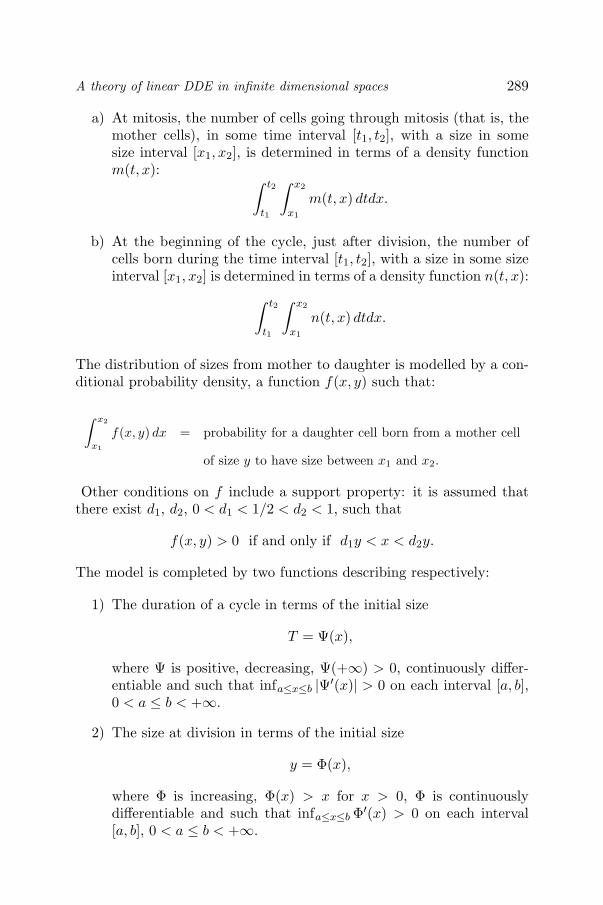
A theory of linear DDE in infinite dimensional spaces
a) At mitosis, the number of cells going through mitosis (that is, themother cells), in some time interval [t1, t2], with a size in somesize interval [x1, x2], is determined in terms of a density functionm(t, x): ∫ t2
t1
∫ x2
x1
m(t, x) dtdx.
b) At the beginning of the cycle, just after division, the number ofcells born during the time interval [t1, t2], with a size in some sizeinterval [x1, x2] is determined in terms of a density function n(t, x):
∫ t2
t1
∫ x2
x1
n(t, x) dtdx.
The distribution of sizes from mother to daughter is modelled by a con-ditional probability density, a function f(x, y) such that:
∫ x2
x1
f(x, y) dx = probability for a daughter cell born from a mother cell
of size y to have size between x1 and x2.
Other conditions on f include a support property: it is assumed thatthere exist d1, d2, 0 < d1 < 1/2 < d2 < 1, such that
f(x, y) > 0 if and only if d1y < x < d2y.
The model is completed by two functions describing respectively:
1) The duration of a cycle in terms of the initial size
T = Ψ(x),
where Ψ is positive, decreasing, Ψ(+∞) > 0, continuously differ-entiable and such that infa≤x≤b |Ψ′(x)| > 0 on each interval [a, b],0 < a ≤ b < +∞.
2) The size at division in terms of the initial size
y = Φ(x),
where Φ is increasing, Φ(x) > x for x > 0, Φ is continuouslydifferentiable and such that infa≤x≤b Φ′(x) > 0 on each interval[a, b], 0 < a ≤ b < +∞.
289

DELAY DIFFERENTIAL EQUATIONS
From these basic assumptions, one can derive two fundamental equa-tions relating the state functions n and m (see [24]). Eliminating m fromthe two equations leads to
n(t, x) = 2∫ +∞
0f (x, Φ(y)) n (t−Ψ(y), y) dy. (1.3)
The assumption on the support of f induces a support property for n;that is, if we assume that n(s, x) = 0 for all x outside an interval [A1, A2],0 < A1 ≤ A2 < +∞, and s < t, then equation (1.3) yields:
n(t, x) = 0 for x < d1Φ(A1) or x > d2Φ(A2).
Assuming that
d1Φ′(0) > 1 and d2 lim supx→+∞
Φ(x)x
< 1,
we deduce from the above remark that for any A1 > 0 small enough,and A2 < +∞, large enough, the size interval [A1, A2] is invariant, thatis, all generations of cells born from cells with initial size in [A1, A2] willhave size at birth in the same interval. Note that for such cells the cellcycle length is bounded above by the number
r = Ψ(A1). (1.4)
Assuming all the above conditions hold, choosing A1, A2 as we just said,r being given by formula (1.4), it was proved in [24] that equation (1.3)yields a positive semigroup in the space
E = L1 ((−r, 0)× (A1, A2)) ,
that is, the one parameter family of maps which to any initial functionp ∈ E associates the function denoted nt, t ≥ 0:
nt(θ, x) := n(t + θ, x) , −r ≤ θ < 0 , x ∈ (A1, A2),
with n0 = p, where n verifies equation (1.3)) for all t ≥ 0, determines astrongly continuous semigroup of positive operators on E ([84]) which,moreover, are compact for t large enough.
As a brief comment on the original proof of this result, let us pointout that the right-hand side of (1.3) is explicitly determined in termsof the initial function p, for all 0 < t < Ψ(A2). So, the solution canbe computed on the set (0, Ψ(A2)) × (A1, A2) by a straight integrationof the initial function. Then, taking nψ(A2) as a new initial function,
290

A theory of linear DDE in infinite dimensional spaces
the solution can be computed on (Ψ(A2), 2Ψ(A2)) × (A1, A2); then, byinduction, it can be computed on each set (kΨ(A2), (k + 1)Ψ(A2)) ×(A1, A2) for each k ≥ 1.
Note that the principle of integration of such equations is the sameas in the case of difference equations. Thus, computing the solutions isalmost a trivial task, the only not completely obvious thing being thatthe function defined by putting end to end the pieces corresponding toeach set (kΨ(A2), (k + 1)Ψ(A2))× (A1, A2) verifies equation (1.3) for allt > 0.
In [3], [4], [5], nonlinear extensions of equation (1.3) were introduced.We will mention only one such model ([5]):
n(t, x) = 2λσ (N(t− τ))∫ +∞
0f (x, Φ(y)) n (t−Ψ(y), y) dy, (1.5)
where
N(t) =∫ +∞
0
(∫ t
t−Ψ(x)n(s, x) ds
)dx, (1.6)
N(t) represents the number of cells present at time t. The expressionλσ (N(t− τ)) models a control mechanism which can be interpreted as arate of defective division. This rate is shaped by the function σ, assumedto be C1, and decreasing, 0 < σ(x) < 1; λ is a coefficient of magnitude0 < λ < 1. As λ increases from 0 to 1, σ being unchanged, stabilityproperties of equilibria of equation (1.5) may change. In [3], the caseτ = 0 was studied. It was proved that for λ less than some value, thesolutions converge to zero, while, above this value, zero loses its stabilityand a new global equilibrium arises. In the case τ > 0, the problem isfar more complicated. In [5] some global results regarding the existenceof slowly oscillating periodic solutions were obtained, in very restrictedsituations.
A reasonable conjecture is that these large oscillations are precededby small periodic oscillations taking place in the vicinity of the nontrivialequilibrium, due to a local Hopf bifurcation.
One of the main motivations of our effort in the direction of abstractdelay equations lies in the fact that we aimed at investigating the aboveconjecture. For this purpose, the difference equation approach is notwell-suited.
291

DELAY DIFFERENTIAL EQUATIONS
1.3 From integro-difference to abstract delaydifferential equations ([8])
1.3.1 The linear equation. We will now derive two differ-ential equations from equation (1.3). The first one leads to a partialdifferential equation with retarded arguments, a retarded version of theLotka-Volterra equation of demography ([42]). The theory underlyingsuch an equation is the theory of abstract delay differential equationswith unbounded operators. Although it is probably the best frameworkin the sense that it leads to the same semigroup as equation (1.3), itinvolves a theory that is not available yet. The second one is a differ-ential equation with retarded arguments and a bounded operator. Itfits into the framework within which the extension of the theory of de-lay differential equations will be developed later ([58], [7]). The mainshortcoming of the second equation is that it leads to a dynamical sys-tem much bigger than the one under study, one in which the solutionsof interest determine a proper subset. However, some of the dynamicalproperties of the larger system also hold for the smaller one, for example,stability and bifurcation of equilibria in the larger system reflect similarproperties for the smaller one. This fact amply justifies in our view thestudy of this system which, on the other hand, is much simpler than thesmaller one.
Retarded partial differential equation formulation of equa-tion (1.3).– Consider a solution n of equation (1.3). Assume that n canbe differentiated with respect to time and size. We will use the notations∂1n (resp. ∂2n) to denote the function obtained by taking the partialderivative of n with respect to its first variable (resp. the second one).The computations we will perform are mostly formal. They could bejustified afterwards.
Taking the derivative with respect to t on both sides of equation (1.3),we arrive at
∂n
∂t= 2∫ +∞
0f (x,Φ(y)) (∂1n) (t−Ψ(y), y) dy.
We have
∂
∂y[n (t−Ψ(y), y)] = −Ψ′(y)∂1n (t−Ψ(y), y) + ∂2n (t−Ψ(y), y) ,
from which we deduce the following expression for ∂1n:
(∂1n) (t−Ψ(y), y) = − 1Ψ′(y)
[∂
∂y[n (t−Ψ(y), y)]− ∂2n (t−Ψ(y), y)
].
292

A theory of linear DDE in infinite dimensional spaces
Inserting the right-hand side of the above in the expression of ∂n/∂t, weobtain
∂n
∂t(t, x) = −2
∫ +∞
0
f (x,Φ(y))Ψ′(y)
∂
∂y[n (t−Ψ(y), y)] dy
+2∫ +∞
0
f (x,Φ(y))Ψ′(y)
∂2n (t−Ψ(y), y) dy.
At this point, we remind the reader that we work with functions n(t, x)whose support in x is contained in [A1, A2], that is, n(t, x) = 0 for x < A1
or x > A2.If we assume further that
∂
∂y
[f (x,Φ(y))
Ψ′(y)
]exists inL1
((A1, A2)2
), (1.7)
then we can use integration by parts on the first integral in the aboveexpression of ∂n/∂t, which yields the following
∂n
∂t(t, x) = 2
∫ +∞
0
∂
∂y
[f (x,Φ(y))
Ψ′(y)
]n (t−Ψ(y), y) dy
+2∫ +∞
0
f (x, Φ(y))Ψ′(y)
∂2n (t−Ψ(y), y) dy. (1.8)
If, conversely, we start from equation (1.7), and integrate it to get backto equation (1.3), then, in fact, we obtain:
n(t, x)− n(0, x) = 2∫ +∞
0f (x, Φ(y)) [n (t−Ψ(y), y)− n (−Ψ(y), y)] dy.
So, in order to come back to equation (1.3), it is necessary to complementthe partial differential equation with the boundary condition
n(0, x) = 2∫ +∞
0f (x,Φ(y)) n (−Ψ(y), y) dy. (1.9)
Equation (1.7) is a sort of functional transport equation, an extensionof the Lotka-von Foerster equation for age-dependent populations ([42]),or the Bell-Anderson equation ([13]) for size-dependent cell populations.The term
2∫ +∞
0
f (x, Φ(y))Ψ′(y)
∂2n (t−Ψ(y), y) dy
corresponds to ∂l/∂a(t, a) in the classical Sharpe-Lotka model of de-mography, or ∂/∂x (g(x)p(t, x)) in the cell population model ([13]). Thequantity
−2∫ +∞
0
∂
∂y
[f (x,Φ(y))|Ψ′(y)|
]n (t−Ψ(y), y) dy
293

DELAY DIFFERENTIAL EQUATIONS
accounts for the mortality term.We summarize the relationship between the integro-difference equa-
tion and the P.D.E. as follows:
Proposition 36 Assume all the above stated conditions on f , Φ andΨ, including condition given by formula ( 1.7). Then, equation ( 1.3) isequivalent to the system ( 1.7)-( 1.9).
Delay differential equation formulation of equation (1.3).– Ifin equation (1.3) we let t > r, we can express n (t−Ψ(y), y) in integralform. This leads to the equation
n(t, x) = 4∫ +∞
0
∫ +∞
0f (x,Φ(y)) f (y, Φ(z)) n (t−Ψ(y)−Ψ(z), z) dzdy.
(1.10)Assuming that n can be differentiated with respect to t, and taking thederivative of (1.10) on both sides, we arrive at
∂n
∂t= 4∫ +∞
0
∫ +∞
0f (x,Φ(y)) f (y, Φ(z)) ∂1n (t−Ψ(y)−Ψ(z), z) dzdy.
The quantity ∂1n (t−Ψ(y)−Ψ(z), z) can be interpreted as the deriva-tive with respect to y:
∂1n (t−Ψ(y)−Ψ(z), z) = − 1Ψ′(y)
∂
∂y[n (t−Ψ(y)−Ψ(z), z)] .
Once again, integration by parts using the fact that n(t, ·) has supportin [A1, A2], yields the desired equation:
∂n
∂t(t, x) = 4
∫ +∞
0
∫ +∞
0
∂
∂y
[f (x, Φ(y)) f (y, Φ(z))
Ψ′(y)
]n (t − Ψ(y) − Ψ(z), z) dzdy,
(1.11)
provided that we assume
∂
∂y
[f (x, Φ(y)) f (y, Φ(z))
Ψ′(y)
]exists in L1
((A1, A2)3
).
Denoting L the linear operator:
L : C([−2r, 0]; L1(A1, A2)
)−→ L1(A1, A2)
defined by the right-hand side of equation (1.11):
(Lp)(x) := 4
∫ +∞
0
∫ +∞
0
∂
∂y
[f (x, Φ(y)) f (y, Φ(z))
Ψ′(y)
]p (−Ψ(y) − Ψ(z), z) dzdy,
294

A theory of linear DDE in infinite dimensional spaces
equation (1.11) reads
∂n
∂t= L(nt). (1.12)
Equation (1.12) is an example of what we call abstract linear delay dif-ferential equations. If, conversely, n is a solution of (1.12), integratingthe equation on both sides from 0 to t we obtain, after integration byparts:
n(t, x) − n(0, x) = 4
∫ +∞
0
∫ +∞
0f (x, Φ(y)) f (y, Φ(z)) n (t − Ψ(y) − Ψ(z), z) dzdy
−4
∫ +∞
0
∫ +∞
0f (x, Φ(y)) f (y, Φ(z)) n (−Ψ(y) − Ψ(z), z) dzdy.
If we assume that
n(0, x) = 4∫ +∞
0
∫ +∞
0f (x, Φ(y)) f (y, Φ(z)) n (−Ψ(y)−Ψ(z), z) dzdy ,
(1.13)then the same equality holds for all t > 0, that is
n(t, x) = 4∫ +∞
0
∫ +∞
0f (x, Φ(y)) f (y, Φ(z)) n (t−Ψ(y)−Ψ(z), z) dzdy .
(1.14)Equation (1.14) is strictly more general, however, than equation (1.3),and leads to a much bigger set of solutions than the one determined by(1.3).
A very partial converse result in this respect is the following: if n is asolution of equation (1.14) and, for some t0, n satisfies (1.3) for all t in(t0, t0 + r), then n satisfies (1.3) for all t > t0.
1.3.2 Delay differential equation formulation of system (1.5)-(1.6) . Note that in the case of system (1.5)-(1.6), the maxi-mum delay is τ + r. If, in equation (1.5) we let t > r, we can expressn (t−Ψ(y), y) in integral form. This leads to the equation:
n(t, x) = 4λ2σ (N(t− τ))∫ +∞
0
∫ +∞
0f (x,Φ(y)) f (y, Φ(z))×
×σ (N (t−Ψ(y)− τ))n (t−Ψ(y)−Ψ(z), z) dzdy.(1.15)
295

DELAY DIFFERENTIAL EQUATIONS
Assuming that n can be differentiated with respect to t, and taking thederivative with respect to t on both sides of (1.14), we obtain:
∂n
∂t(t, x) = σ′ (N(t − τ)) N(t − τ)
n(t, x)
σ (N(t − τ))
+4λ2σ (N(t − τ))
∫ +∞
0
∫ +∞
0f (x, Φ(y)) f (y, Φ(z)) ×
× ∂
∂t[σ (N (t − Ψ(y) − τ)) n (t − Ψ(y) − Ψ(z), z)] dzdy. (1.16)
We point out the fact that N can indeed be differentiated, and:
N(t) =∫ +∞
0[n(t, x)− n (t−Ψ(x), x)] dx. (1.17)
We note the same property as in the previous computation:
∂
∂t[σ(N(t−Ψ(y)− τ))n(t−Ψ(y)−Ψ(z), z)]
= − 1Ψ′(y)
∂
∂y[σ (N (t−Ψ(y)− τ)) n (t−Ψ(y)−Ψ(z), z)] .
Integration by parts with respect to y of the last integral on the right-hand side of (1.15) transforms this integral into
4λ2σ (N(t− τ))∫ +∞
0
∫ +∞
0
∂
∂y
[f (x,Φ(y)) f (y, Φ(z))
Ψ′(y)
]×
×σ (N (t−Ψ(y)− τ))n (t−Ψ(y)−Ψ(z), z) dzdy.
Using the above expression and formula (1.17), equation (1.15) yieldsthe following
∂n
∂t(t, x) =
σ′ (N(t − τ))
σ (N(t − τ))n(t, x)
∫ +∞
0[n(t − τ, y) − n (t − τ − Ψ(y), y)] dy
+4λ2σ (N(t − τ))
∫ +∞
0
∫ +∞
0
∂
∂y
[f (x, Φ(y)) f (y, Φ(z))
Ψ′(y)
]×
×σ (N (t − Ψ(y) − τ)) n (t − Ψ(y) − Ψ(z), z) dzdy. (1.18)
Assume that n(t, ·) is defined on R (for example, n is a periodic solutionof (1.5)). In this case, n satisfies equation (1.14). Assuming f boundedon bounded rectangles, we conclude that n is bounded and continuouson each set [−T, T ] ×R+, (T > 0), which in particular implies that Nis locally Lipschitz continuous. Assuming moreover that f is C1, it ispossible to write the integral in equation (1.14) in the following way:∫ A2
A1
∫ t−Ψ(A1)
t−Ψ(A2)f(x,Φ
(Ψ−1(t− s)
))f(Ψ−1(t− s),Φ(z)
)×
296

A theory of linear DDE in infinite dimensional spaces
×σ (N(s− τ)) n (s−Ψ(z), z) |(Ψ−1)′(t− s)| dsdz ,
which implies that n is locally Lipschitz in t, uniformly in x, in otherwords, there exists N , a negligible set of t-values, such that n(t, x) isdifferentiable for all t not in N , and all x ∈ (A1, A2). In conclusion, wehave the following
Lemma 32 If n is a solution of ( 1.5), defined for every t in R, then nis differentiable in t with ∂n/∂t continuous in R×R, satisfying equation( 1.17).
Equation (1.17) is a nonlinear delay differential equation on the spaceL1(A1, A2), with maximum delay equal to 2r + τ . As in the linear case,it is obvious, by construction, that the solutions of the system (1.5)-(1.6)are solutions of equation (1.17), but equation (1.17) has a much biggerset of solutions than system (1.5)-(1.6). The motivation for embeddingthe latter system into a bigger one is that the framework of differentialequations seems to be more suited to the study of dynamical featuressuch as stability than the framework of integral equations.
1.4 The linearized equation of equation (1.17)near nontrivial steady-states
Equation (1.17) is the most complete of all the equations consideredhere. It can be reduced to equation (1.11) by assuming that 2λσ(N) =1. If the delay τ = 0, we obtain the equation studied in [3]. Ourprogram regarding equation (1.17) is to start from the steady-states andinvestigate their stability and the loss of stability in terms of λ. Whilewe already know from [3] that stability passes from a constant steady-state to another one when τ = 0, we expect that in the delay case stableoscillations may take place. This fact has been shown under severalrestrictions in [5]: existence of periodic slowly oscillating solutions hasbeen demonstrated for a range of values of the parameters. However, theresult is not explicitly related to any bifurcation of steady-state periodicsolution. We believe however that there is a strong possibility that sucha bifurcation occurs at these values of λ where some eigenvalues of thelinearized equation cross the imaginary axis (away from zero).
1.4.1 The steady-state equation. Note that any functionn(x) of x only verifies equation (1.17) trivially. If n = n, we have
N(t) = N =∫ +∞
0Ψ(x)n(x) dx.
297

DELAY DIFFERENTIAL EQUATIONS
From them we will only retain those which are non-negative solutions ofthe system (1.5)-(1.6). Equation (1.5) leads to
n(x) = 2λσ(N)∫ +∞
0f (x,Φ(y)) n(y) dy.
Integrating the above equation on both sides and using the fact thatf (·, Φ(y)) is a probability density, we obtain
2λσ(N) = 1
and
n(x) =∫ +∞
0f (x,Φ(y)) n(y) dy. (1.19)
Equation (1.19) is, notably, dealt with in detail in [2]. It is a typical ex-ample of application of the Perron-Frobenius theory of positive operatorson ordered Banach spaces.
Equation (1.19) has a unique positive solution n1 such that∫ +∞0 n1(x) dx = 1.
In terms of n1, n = kn1, where k is a constant. The constant k satisfiesthe relation
2λσ
(k
∫ +∞
0Ψ(x)n1(x) dx
)= 1. (1.20)
Assuming that
σ(0) >12
; σ(+∞) = 0,
equation (1.20) has, for each λ >1
2σ(0), one and only one root k = k(λ).
The function k is increasing.
1.4.2 Linearization of equation (1.17) near (n, N) . Thelinearization is obtained by formally differentiating equation (1.17) withrespect to every occurrence of n as if it were an independent variableand multiplying the result by the same occurrence of the variation ∆n.This yields the following:
∂
∂t(∆n)(t, x) =
σ′(N)
σ(N)n(x)
∫ +∞
0[(∆n)(t − τ, y) − (∆n)(t − τ − Ψ(y), y)] dy
+4λ2σ(N)
∫ +∞
0
∫ +∞
0
∂
∂y
[f (x, Φ(y)) f (y, Φ(z))
Ψ′(y)
]×
×[σ′(N)∆N(t − Ψ(y) − τ)n(z)
+σ(N)∆n (t − Ψ(y) − Ψ(z), z)]
dzdy.
298

A theory of linear DDE in infinite dimensional spaces
The equation can be simplified a little bit. In view of relation (1.19),we have
∫ +∞
0
∫ +∞
0
∂
∂y
[f (x, Φ(y)) f (y, Φ(z))
Ψ′(y)
]n(z)dzdy =
∫ +∞
0
∂
∂y
[f (x, Φ(y)) n(y)
Ψ′(y)
]dy.
This, in turn, leads to∫ +∞
0
∫ +∞
0
∂
∂y
[f (x, Φ(y)) f (y, Φ(z))
Ψ′(y)
]∆N (t − Ψ(y) − τ) n(z) dzdy
=
∫ +∞
0
∂
∂y
[f (x, Φ(y)) n(y)
Ψ′(y)
]∆N (t − Ψ(y) − τ) dy
=
∫ +∞
0
f (x, Φ(y)) n(y)∂1(∆N) (t − Ψ(y) − τ) dy
=
∫ +∞
0
f (x, Φ(y)) n(y) ×
×[∫ +∞
0
[(∆n) (t − Ψ(y) − τ, z) − (∆n) (t − Ψ(y) − Ψ(z) − τ, z)] dz
]dy.
We arrive at the following equation
∂
∂t(∆n)(t, x) =
σ′(N)
σ(N)n(x)
∫ +∞
0[(∆n)(t − τ, y) − (∆n) (t − τ − Ψ(y), y)] dy
+2λσ′(N)
∫ +∞
0f (x, Φ(y)) n(y) ×
×[∫ +∞
0[(∆n) (t − Ψ(y) − τ, z) − (∆n) (t − Ψ(y) − Ψ(z) − τ, z)] dz
]dy
+
∫ +∞
0
∫ +∞
0
∂
∂y
[f (x, Φ(y)) f (y, Φ(z))
Ψ′(y)
](∆n) (t − Ψ(y) − Ψ(z), z) dzdy.
(1.21)
1.4.3 Exponential solutions of (1.20) . The study of thestability of n as a solution of equation (1.17) amounts to the study ofthe growth rate of the semigroup associated to equation (1.20). In thecase of a compact or eventually compact semigroup, this amounts todetermining exponential solutions (exp zt)x. Then, the growth rate isnegative if sup Re z < 0, and it is positive if sup Re z > 0. Bifurcationof equilibria occurs at the values of parameters where the growth ratechanges signs. It can be shown that the semigroup associated to equation(1.20) is not eventually compact, but its restriction to the elements of
299

DELAY DIFFERENTIAL EQUATIONS
C ([−r, 0]; X) satisfying (1.13) is. This remark motivates the study ofexponential solutions of equation (1.20).
Let ν(t, x) = eztp(x) be a solution of equation (1.20). Substitutingeztp(x) for ∆n in (1.20) yields
zp(x) = e−zτ σ′(N)
σ(N)n(x)
∫ A2
A1
(1 − e−zΨ(y)
)p(y) dy
+2λσ′(N)
∫ A2
A1
f (x, Φ(y)) n(y) ×
×[∫ A2
A1
e−z(Ψ(y)+τ)(1 − e−zΨ(u)
)p(u) du
]dy
+
∫ A2
A1
∫ A2
A1
∂
∂y
[f (x, Φ(y)) f (y, Φ(u))
Ψ′(y)
]e−z(Ψ(y)+Ψ(u))p(u)dudy.
(1.22)
To abbreviate, we will call such an equation a spectral equation. Notethat the right-hand side of the above equation vanishes for z = 0. Forthis value of z, every function p satisfies the equation. Equation (1.21)is quite complicated. We will not study it directly. Instead, we willnow introduce the eigenvalue equation associated with the linearizationof equation (1.5). Then, we will show that both equations are partiallyequivalent to each other.
Ideally, one could expect that this part of the spectrum is the partbrought up by the passage from the integral to the differential formu-lation, and the remaining part of the spectrum reflects the spectrumof the integral equation only. The spectral equation associated to thelinearization of equation (1.5) near n is
p(x) = e−zτ2λσ′(N)
(∫ A2
A1
p(y)
(1− e−zΨ(y)
z
)dy
)n(x)
+∫ A2
A1
f (x, Φ(y)) e−zΨ(y)p(y) dy. (1.23)
One can easily verify that every solution of equation (1.22) is also asolution of equation (1.21). In the following Lemma, we state a partialconverse of this result.
Lemma 33 Denote σ1 (resp. σ2 ) the set of complex numbers z, z = 0,Re z ≥ 0, such that equation ( 1.21) (resp.) ( 1.22) ) has a nonzerosolution for the value z. Then, σ1 = σ2.
300

A theory of linear DDE in infinite dimensional spaces
Moreover, for each z ∈ σi, let N iz ( i = 1, 2) be the space of functions
p such that p is a solution of ( 1.21) (resp. ( 1.22) ) for the value z.Then, N 1
z = N 2z.
Proof.– For each z = 0, we introduce the operators
Bz(p) := 2λσ′(N)∫ A2
A1
p(y)
[1− e−zΨ(y)
z
]dy,
(Lzp) (x) :=∫ A2
A1
f (x,Φ(y)) e−zΨ(y)p(y) dy.
Then equation (1.22) is
p(x) = e−zτn(x)Bz(p) + (Lzp) (x),
and equation (1.21) reads
p(x) = e−zτn(x)Bz(p) + (Lzq) (x),
whereq(x) = e−zτn(x)Bz(p) + (Lzp) (x).
We need only prove that p, a solution of (1.21) for some z = 0, withRe z ≥ 0, satisfies (1.22) for the same value of z. But this is equivalentto proving p = q. Since we have
p(x)− q(x) = (Lz(p− q)) (x),
and the equationp(x) = (Lzp) (x)
can be satisfied with p = 0 only if Re z < 0, the Lemma follows.
We will now briefly discuss equation (1.22).For z = 0, equation (1.22) reduces to
p(x) = 2λσ′(N)(∫ A2
A1
p(y)Ψ(y) dy
)n(x)
+∫ A2
A1
f (x, Φ(y)) p(y) dy,
which has p = 0 as the only solution.In fact, integrating the above equation on both sides on (A1, A2), we
obtain
2λσ′(N)(∫ A2
A1
p(y)Ψ(y) dy
)= 0,
301

DELAY DIFFERENTIAL EQUATIONS
which implies that
p(x) =∫ A2
A1
f (x, Φ(y)) p(y) dy,
and therefore, in view of (1.19):
p(x) = kn(x).
So,
0 =∫ A2
A1
p(y)Ψ(y) dy = k
∫ A2
A1
n(y)Ψ(y) dy.
This, with the fact n > 0, implies that k = 0, that is p = 0.For z = 0, integrating equation (1.22) on both sides on (A1, A2), we
obtain[∫ A2
A1
p(y)(1− e−zΨ(y)
)dy
] [2λσ′(N)e−zτ
(∫ A2
A1
n(y) dy
)− z
]= 0.
(1.24)Equation (1.24) breaks down into two equations
∫ A2
A1
p(y)(1− e−zψ(y)
)dy = 0, (1.25)
zezτ = 2λσ′(N)∫ A2
A1
n(y) dy. (1.26)
Assuming (1.25) holds, equation (1.22) yields, with z = 0:
p(x) =∫ A2
A1
f (x,Φ(y)) e−zΨ(y)p(y) dy,
which can be satisfied with p = 0 only if Re z < 0.So, instability from nonzero roots crossing the imaginary axis can only
come from roots of equation (1.26). We have the following result:For each λ > 0, equation (1.24) has a pair of nonzero roots crossing
the imaginary axis at each value τ = τk, where
τk =π/2 + 2kπ
2λ|σ′(N)|∫ A2
A1n(y) dy
, k ∈ N.
Once equation (1.24) has been solved for z = 0, in order to have a fullsolution of equation (1.21), it remains to solve equation (1.22) for p.
The equation can be written in the form
(I −K)p = 0,
302

A theory of linear DDE in infinite dimensional spaces
where K is a compact operator. The fact that
∫ A2
A1
([I −K]p) (x) dx = 0
for every p ∈ X, implies that Im (I −K) is a proper subspace of X, andtherefore, by virtue of a well known property of compact operators, thenull set of I −K is not reduced to 0.
1.5 ConclusionThe construction of a theory of delay differential equations in infinite
dimensional spaces is motivated by the study of some integro-differenceequations arising in some models of cell population dynamics. The in-troduction of a nonlinearity in these models to account for possible self-regulating control mechanism of cell number suggested possible oscilla-tions. The integro-difference nature of the model did not allow the useof any known standard techniques to exhibit such oscillations.The ob-servation that was made that this system (and its solutions) can in factbe viewed as solutions of a larger system of delay differential equationsin an infinite dimensional space led to the idea to extend this frame themachinery for the study of stability that has been developed for delaydifferential equations in finite dimensional spaces.
Let us conclude with a few comments about oscillations. Oscillationwith respect to time of the number of cells is a recognized fact in severalexamples, among which is the production of red blood cells ([4], [17]).This phenomenon can also be observed in cultured cells. It used to be acommon belief that such oscillations reflect the role of delays at variousstages of the life of cells. A lot of efforts were made during the seventiesin the study of homogeneous nonstructured models with the goals offirst proving existence of periodic oscillations, after that counting themand looking at their stability and other properties. Amongst those whocontributed to these works let us mention [12], [22] and [41]. In contrastto this, very little has been done in the case of structured models. One ofthe reasons is that there is no general theory for the study of dynamicalproperties of such equations. The theory on abstract D.D.E. that wepresent here is a step in this direction.
2. The Cauchy Problem For An Abstract LinearDelay Differential Equation
Our interest in functional differential equations in infinite dimensionsstemmed from the study of the dynamical properties of such equations
303

DELAY DIFFERENTIAL EQUATIONS
and the remark we made at some point that it is possible to associateto any of them a delay differential equation on an infinite dimensionalvector space. We start with this theory for the linear and autonomouscase and this section is devoted to the resolution of the Cauchy problem.
We start setting up the general framework of the equations understudy. The notation C stands for the space C([−r, 0]; E) (r > 0) of thecontinuous functions from the interval [−r, 0] into E, E being a realBanach space, endowed with the sup norm
‖ϕ‖C := supθ∈[−r,0]
‖ϕ(θ)‖E .
Let L : C −→ E be a bounded linear operator. We are considering thefollowing Cauchy problem for the delay equation defined by the operatorL:
For each ϕ ∈ C, to find a function x ∈ C([−r, +∞[; E), x ∈ C1([0, +∞[; E) such that the following relations hold
(CP )
x′(t) = L(xt) , for all t > 0x0 = ϕ
As usual, xt denotes the section at t of the function x, namely xt(θ) :=x(t + θ), θ ∈ [−r, 0]. The Cauchy problem is well-posed if it has one andonly one solution for each initial value ϕ.
2.1 Resolution of the Cauchy problemThere are several ways to solve problem (CP). The most elementary
one is to write the equation in integral form
x(t) = x(0) +∫ t
0L(xs) ds , t > 0. (2.1)
Define the function ϕ0 : [−r, +∞[−→ E by
ϕ0(t) :=
ϕ(t) if t ∈ [−r, 0]ϕ(0) if t ≥ 0.
The change of x by the unknown function
y(t) := x(t)− ϕ0(t)
transforms equation (2.1) into
y(t) =∫ t
0L(ys) ds +
∫ t
0L(ϕ0
s) ds (2.2)
304

A theory of linear DDE in infinite dimensional spaces
which can be formulated as an abstract equation in a suitable framework.To this end, for each α > 0 let us define
Eα0 := y ∈ C([0, +∞); E) ; y(0) = 0 , ‖y‖α := sup
t≥0e−αt‖y(t)‖E < +∞
which is a Banach space with respect to the norm ‖ · ‖α.Let Q be the bounded linear operator defined by
Q : E0α −→ E0
α ; (Qy)(t) :=∫ t
0L(ys) ds
where y is the extension by zero of function y to [−r, 0]. In terms of thisoperator, equation (2.2) reads as:
(Id−Q)(y)(t) =∫ t
0L(ϕ0
s) ds.
The norm of Q on Eα0 satisfies the following estimate
‖Qy‖α ≤‖L‖α‖y‖α
so, for α > ‖L‖, Q is a strict contraction. This implies that equation(2.1) has one and only one solution defined on [−r, +∞[. This provesthat the Cauchy problem (CP) is well-posed.
As usual, bearing in mind that the initial state is the function ϕ andthe state at time t is the function xt, we introduce the solution operatorT (t) defined by
T (t)ϕ := xt , t > 0.
It is easy to check that the family T (t)t≥0 is a strongly continuoussemigroup of linear bounded operators on C. An obvious property ofthis semigroup is that
[T (t)ϕ] (θ) =
ϕ(t + θ) if t + θ ≤ 0[T (t + θ)ϕ] (0) if t + θ ≥ 0
that is, T (t)t≥0 is a translation semigroup.
Straightforward computation leads to the following operator as theinfinitesimal generator of the semigroup:
Aϕ := ϕ (2.3)
with domain
D(A) = ϕ ∈ C1([−r, 0]; E) ; ϕ(0) = L(ϕ). (2.4)
305

DELAY DIFFERENTIAL EQUATIONS
2.2 Semigroup approach to the problem (CP)Semigroups defined on some functional space of the type F(J ; E),
where J is an interval and F is some class of functions (continuousfunctions, Lp functions, etc) and with infinitesimal generator A definedby the derivative on J , have been investigated by several authors aftera pioneering work by A. Plant [34]. Extension of Plant’s results toabstract delay differential equations can be found in [16] and in [73].The following result is borrowed from [73].
Theorem 1 The operator A defined by ( 2.3) with domain given by( 2.4) is the infinitesimal generator of a strongly continuous semigroupS(t)t≥0 on C satisfying the translation property
(S(t)ϕ)(θ) =
ϕ(t + θ) if t + θ ≤ 0(S(t + θ)ϕ)(0) if t + θ > 0
t > 0, θ ∈ [−r, 0], ϕ ∈ C. Furthermore, for each ϕ ∈ C, define x :[−r, +∞) −→ E by
x(t) :=
ϕ(t) if t ∈ [−r, 0](S(t)ϕ)(0) if t > 0.
Then x is the unique solution of (CP) and S(t)ϕ = xt, t > 0.
Remark 1.– The last part of the theorem states that in fact S(t) =T (t), t ≥ 0, which we can assert as soon as we know that S(t)t≥0 andT (t)t≥0 are both associated with the same infinitesimal generator.
Proof.– In order to illustrate the type of computations and ideas in-volved in delay equations, we will briefly sketch the proof of the theorem.
First of all, we will check that A is the infinitesimal generator of astrongly continuous semigroup. Using the Lumer-Phillips version of theHille-Yosida theorem, we have to prove that:
i) A is a closed operator with a dense domain.
ii) The resolvent operator
R(λ, A) := (λI −A)−1
exists, for all real λ large enough and there exists a real constantω such that
‖(λI −A)−1‖ ≤ 1λ− ω
; λ > ω.
306

A theory of linear DDE in infinite dimensional spaces
We skip (i), which is obvious. In order to prove (ii), given f ∈ C we haveto solve
(λI −A)ϕ = f ; ϕ ∈ D(A). (2.5)
The resolution of (2.5), which is straightforward, leads to
ϕ(θ) = eλθϕ(0) +∫ 0
θeλ(θ−s)f(s) ds. (2.6)
In order to verify that ϕ ∈ D(A), we have to check the boundary condi-tion for ϕ:
λϕ(0)− f(0) = L
(eλ·ϕ(0) +
∫ 0
·eλ(·−s)f(s) ds
). (2.7)
Let us introduce the following bounded linear operators
Lλ : E −→ E ; Lλ(z) := L(ελ ⊗ z)
where ελ ⊗ z ∈ C([−r, 0]; E) is defined by
(ελ ⊗ z)(θ) := eλθz , θ ∈ [−r, 0]
and Sλ : C −→ E defined by
Sλ(f) = f(0) + L
(∫ 0
·eλ(·−s)f(s) ds
). (2.8)
Lemma 34 For each λ ∈ C, the operator Sλ is onto.
Proof.–Let us consider the family of bounded linear operators Σλ,kk=1,2,... ⊂ L(E)
defined byΣλ,k(z) := Sλ (χk ⊗ z)
where(χk ⊗ z)(θ) := χk(θ)z , θ ∈ [−r, 0]
and χkk=1,2,... is the family of real functions defined by
χk(θ) := max(
kθ
r+ 1 , 0
), θ ∈ [−r, 0].
It is easily seen that for each λ, the sequence of operators Σλ,k convergesin operator norm towards the identity. Therefore Σλ,k is invertible for klarge enough.
307

DELAY DIFFERENTIAL EQUATIONS
In terms of Σλ,k, we can build a right inverse of Sλ. To this end, letus define Υλ,k ∈ L(E, C) by
∀b ∈ E , Υλ,k(b) := χk ⊗ Σ−1λ,k(b). (2.9)
It holds thatSλ Υλ,k = IE
where IE is the identity operator on E. This proves our claim.
In terms of operators Lλ and Sλ, we have the following characteriza-tion for λ to belong in the resolvent set of the operator A:
Proposition 37 A necessary and sufficient condition for λ ∈ ρ(A) (re-solvent set of A) is that the operator ∆(λ) defined by
∆(λ) := λI − Lλ
be invertible. Assuming that λ ∈ ρ(A), it holds that
ϕ(0) = ∆(λ)−1Sλ(f)
and, for θ ∈ [−r, 0]:
R(λ, A)(f)(θ) = eλθ∆(λ)−1Sλ(f) +∫ 0
θeλ(θ−s)f(s) ds. (2.10)
To complete the proof of the first part of the theorem it only remainsto obtain a convenient estimate for the norm of R(λ, A).
Straightforward computation shows that the operator Lλ is uniformlybounded on each right half-plane of C (that is, on any set of the typeΩa := z ∈ C ; Re z ≥ a for some a). So, there exists a0 ∈ R such that∆(λ) is invertible all over regions of the complex plane Ωa with a ≥ a0.
Let us defineM := sup
Reλ≥a0
‖Lλ‖.
For any a ≥ a0, we have
Re λ ≥ a =⇒ ‖Lλ‖ ≤M.
So, if we take a > 0 and a ≥ a0 large enough, we will have
λ ≥ a =⇒ ‖Lλ‖λ
< 1
and then‖∆(λ)−1‖ ≤ 1
λ−M.
308

A theory of linear DDE in infinite dimensional spaces
We can also readily check the following estimate for Sλ(f)
‖Sλ(f)‖ ≤(
1 +‖L‖λ
)‖f‖C .
Combining these estimates in formula (2.10) we obtain, for θ ∈ [−r, 0]:
‖ [R(λ, A)f ] (θ)‖E ≤[eλθ
(1 +
‖L‖λ
)1
λ−M+(1− eλθ
) 1λ
]‖f‖C .
Since the quantity inside brackets is a convex combination of two fixedvalues, it is bounded by the maximum of both quantities, from whichwe deduce
‖R(λ, A)‖ ≤ max([
1 +‖L‖λ
]1
λ−M,
1λ
).
To conclude, if we choose ω so that
ω > max(a0 , ‖L‖+ M)
we will have the desired inequality:
‖R(λ, A)‖ ≤ 1λ− ω
for λ > ω.
Translation semigroup property.– It remains to check that thesemigroup S(t)t≥0 enjoys the translation property. To this end, foreach ϕ given in C, let us define the function
x(t) =
[S(t)ϕ] (0) if t ≥ 0ϕ(t) if t ∈ [−r, 0]
What we have to verify is that
S(t)ϕ = xt , t ≥ 0.
Note that the evaluation map ϕ → [S(t)ϕ] (0) is continuous and evenlocally uniformly continuous with respect to t, so the map ϕ → xt iscontinuous for each t ≥ 0, and in fact it is also locally uniformly contin-uous with respect to t. From this remark it follows that we only have toprove the property on a dense subset of initial values. It will extend bycontinuity to all initial values.
So, from this point on, we assume that ϕ ∈ D(A). Then, a basicsemigroup property ensures that S(t)ϕ ∈ D(A) for all t ≥ 0. Therefore
309

DELAY DIFFERENTIAL EQUATIONS
we have that both t → [S(t)ϕ] (θ) and θ → [S(t)ϕ] (θ) are differentiable.Given a pair (t, θ), t ≥ 0, θ ∈ [−r, 0], the function
h → [S(t + h)ϕ] (θ − h)
makes sense as long as t + h ≥ 0 and θ − h ≤ 0, that is, h ≥ max(−t, θ)and can be differentiated on this domain. The derivative is equal to[
d
dtS(t + h)ϕ
](θ − h)− d
dθ[S(t + h)ϕ] (θ − h) = 0.
This implies that [S(t + h)ϕ] (θ − h) is a constant for each fixed pair(t, θ) and h ≥ max(−t, θ).
We now consider two situations:
i) t + θ ≤ 0.In this case, max(−t, θ) = −t. Giving h the values −t and 0, weobtain
[S(t)ϕ] (θ) = ϕ(t + θ) for t + θ ≤ 0.
ii) t + θ ≥ 0.This time, we give h the values θ and 0, which leads to
[S(t)ϕ] (θ) = [S(t + θ)ϕ] (0) for t + θ ≥ 0.
In both cases, we have [S(t)ϕ] (θ) = x(t + θ), according to the definitionof x, therefore, S(t)ϕ = xt, as desired.
2.3 Some results about the range of λI − A
In line with Proposition 37, we have the following results.
Lemma 35 For any λ ∈ C, we have that f ∈ R (λI −A) if and only ifSλ(f) ∈ R (λI − Lλ).
Proof.– It follows immediately from (2.6) and (2.7) combined. For-mula (2.6) shows that the determination of ϕ such that (λI − A)ϕ = famounts to determining ϕ(0) and formula (2.7) gives a necessary andsufficient condition for existence of ϕ(0) which is precisely the conditionstated in the lemma.
Lemma 36 The subspace R (λI − A) is closed in C if and only if thesubspace R (λI − Lλ) is closed in E.
Proof.– First we suppose that R (λI − Lλ) is a closed subspace ofE and let ψnn=1,2,... ⊂ R (λI − A) be a convergent sequence withψ = limn→∞ ψn.
310

A theory of linear DDE in infinite dimensional spaces
From Lemma 35, we have that Sλ(ψn) ∈ R (λI−Lλ) and then Sλ(ψ) ∈R (λI−Lλ). Again Lemma 35 enables us to conclude that ψ ∈ R (λI−A)and so R(λI −A) is closed in C.
Now we are going to demonstrate the converse. We assume thatR (λI−A) is closed and we want to show that it implies that R (λI−Lλ)is closed.
To this end, we recall that Sλ is surjective and that in Lemma 34 wehave exhibited a family of right inverses. Select one such map Υλ,k asdefined by (2.9).
Let bnn=1,2,... be a sequence in E such that the sequence (λI −Lλ)(bn)n=1,2,... converges to some element e ∈ E. Define the sequence
fn := Υλ,k [(λI − Lλ)(bn)] , n = 1, 2, . . .
By construction, we have Sλ(fn) ∈ R (λI − Lλ). Therefore, in view ofLemma 35, we have fn ∈ R (λI − A) and Sλ(fn) = (λI − Lλ)(bn). Wehave also
limn→∞
Sλ(fn) = e ; limn→∞
fn = Υλ,k(e).
R (λI − A) being closed yields that Υλ,k(e) ∈ R (λI − A). Lemma 35again can be invoked to conclude that e = Sλ [Υλ,k(e)] ∈ R(λI − Lλ).The proof is complete.
3. Formal DualityIn this section we present an extension of the formal duality theory
to D.D.E. in infinite dimensional spaces. The presentation follows thework made in [58].
Let us consider the space C∗ := C([0, r]; E∗) where E∗ is the topolog-ical dual space of E. We are going to define a continuous bilinear formdenoted << α, ϕ >> on the product C([0, r]; E∗) × C([−r, 0]; E) whichwill be interpreted as a formal duality.
A function f : [0, r] −→ E∗ is called simple if there exist two finitecollections x∗
1, . . . , x∗p ∈ E∗ and A1, . . . , Ap ∈ Σ with
⋃pi=1 Ai = [0, r],
Ai⋂
Aj = ∅ such that
f =p∑
i=1
x∗i χAi
where χA is the characteristic function of A and Σ is the Borel algebraon [0, r]. Denote S([0, r]; E∗) the space of simple functions.
311

DELAY DIFFERENTIAL EQUATIONS
Definition 37 For any α ∈ S([0, r]; E∗) and ϕ ∈ C([0, r]; E) we definethe bilinear form
<< α, ϕ >>:=< α(0), ϕ(0) > +p∑
i=1
< x∗i , L
(∫ 0
θχAi(ξ − θ)ϕ(ξ) dξ
)>
where α =∑p
i=1 x∗i χAi and < ·, · > denote the usual duality between E∗
and E.
The value << α, ϕ >> is independent of the representation chosen forα as a linear combination of characteristic functions.
Since
| << α, ϕ >> | ≤ (1 + r‖L‖) ‖α‖‖ϕ‖
there exists a unique continuous extension of this bilinear form to thecompletion of S([0, r]; E∗)×C([−r, 0]; E) where both spaces are equippedwith the sup norm.
We restrict our extension to the product C([0, r] : E∗)×C([−r, 0]; E)and we call this the formal duality associated with the operator L.
It is interesting to specify the formal duality for α ∈ C([0, r])⊗ E∗.
Lemma 37 Let f ∈ C([0, r]) and u∗ ∈ E∗. We consider the functionf ⊗ u∗ ∈ C([0, r]; E∗) defined by (f ⊗ u∗) (s) := f(s)u∗, s ∈ [0, r]. Then
<< f⊗u∗, ϕ >>=< u∗, f(0)ϕ(0) > + < u∗, L
(∫ 0
θf(ξ − θ)ϕ(ξ) dξ
)> .
(3.1)
Proof.– The function f is representable as the limit of a uniformlyconvergent sequence of simple real functions defined in [0, r]:
f = limn→∞
pn∑i=1
βi(n)χAi
(n)
and therefore the sequence of functions in S([0, r]; E∗),
pn∑i=1
βi(n)u∗ ⊗ χAi
(n)
n=1,2,...
converges to f ⊗ u∗.
312

A theory of linear DDE in infinite dimensional spaces
By continuity of the formal duality, we obtain
<< f ⊗ u∗, ϕ >>
=< (f ⊗ u∗)(0), ϕ(0) > + limn→∞
pn∑i=1
< βi(n)u∗, L
(∫ 0
θχAi
(n)(ξ − θ)ϕ(ξ) dξ
)>
=< (f ⊗ u∗)(0), ϕ(0) > + limn→∞
pn∑i=1
< u∗, L
(∫ 0
θβi
(n)χAi(n)(ξ − θ)ϕ(ξ) dξ
)>
=< u∗, f(0)ϕ(0) > + < u∗, L
(∫ 0
θf(ξ − θ)ϕ(ξ) dξ
)> .
In particular, introducing the notation ελ(θ) := eλθ, we have
<< ελ ⊗ u∗, ϕ >>=< u∗, ϕ(0) > + < u∗, L
(∫ 0
θeλ(ξ−θ)ϕ(ξ) dξ
)> .
In terms of the operator Sλ defined in (2.8) the above formula reads as
<< ε−λ ⊗ u∗, ϕ >>=< u∗, Sλ(ϕ) > . (3.2)
3.1 The formal adjoint equationBefore proceeding to the construction of this equation let us remind
some well known results about the integral representation of boundedlinear operators defined on C([−r, 0]; E). We refer to [14] for the generaltheory.
Any bounded linear operator L : C([−r, 0]; E) −→ E determines aunique vector measure m : Σ −→ L(E; E∗∗) of bounded semivariationand such that for all f ∈ C([−r, 0]; E) we have
L(f) =∫
[−r,0]fd m
where L(E; E∗∗) is the space of the bounded linear operators definedon E with values in E∗∗, E∗∗ being the bidual of E, and Σ the Borelalgebra on [−r, 0].
For each x∗ ∈ E∗, there exists a vector measure mx∗ : Σ −→ E∗
defined by
< mx∗(A), x >:=< x∗, m(A)(x) > ; A ∈ Σ , x ∈ E
which satisfies∫[−r,0]
fd mx∗ =< x∗, L(f) > ; ∀x∗ ∈ E∗.
313

DELAY DIFFERENTIAL EQUATIONS
Next we define the linear operator L : S([0, r]; E∗) −→ E∗ for any f ∈S([0, r]; E∗), f =
∑pi=1 x∗
i χAi by
L(f) :=p∑
i=1
mx∗i(−Ai).
Lemma 38 If the vector measure m is of bounded variation, then L iscontinuous with respect to the sup norm in S([0, r]; E∗).
Proof.– Let f =∑p
i=1 x∗i χAi be a simple function with ‖x∗
i ‖ ≤ 1,i = 1, . . . , p. Then
‖L(f)‖ = ‖p∑
i=1
mx∗i(−Ai)‖ ≤
p∑i=1
‖mx∗i(−Ai)‖
≤p∑
i=1
‖m(−Ai)‖ ≤ v(m) ([−r, 0]) < +∞
where v(m) means the variation of m and we have used that
‖mx∗i(−Ai)‖ = sup
‖x‖≤1| < mx∗
i(−Ai), x > |
= sup‖x‖≤1
| < x∗i , m(−Ai)(x) > | ≤ ‖m(−Ai)‖.
Under this hypothesis, there exists a unique continuous extension ˜Lof the operator L to the completion of S([0, r]; E∗) equipped with thesup norm and we are able to define the formal adjoint operator of theoperator L.
Definition 38 The operator L∗ is the restriction to the space C∗ of theextension operator ˜L.
Just as we did in the case of the formal duality, it is convenient to ob-tain the expression of L∗ for the elements in C([0, r])⊗E∗. Calculationsvery similar to the ones above for Lemma 37 show that
Lemma 39 For each f ⊗ u∗ ∈ C([0, r]) ⊗ E∗, L∗(f ⊗ u∗) ∈ E∗ is thelinear form defined by
< L∗(f ⊗ u∗), u >:=< u∗, L(f ⊗ u) > ; u ∈ E (3.3)
where f(θ) := f(−θ).
314

A theory of linear DDE in infinite dimensional spaces
For each f ∈ C([−r, 0]), u ∈ E, we have denoted by f ⊗ u the elementof C([−r, 0]; E) defined by
(f ⊗ u)(θ) := f(θ)u , θ ∈ [−r, 0].
In particular, for the functions ε(j)λ defined by
ε(j)λ (θ) :=
θj
j!eλθ ; θ ∈ [−r, 0] , j = 1, 2, . . . (3.4)
we reach the result
< L∗(ε(j)λ ⊗ u∗), u > = < u∗, L(ε(j)
λ ⊗ u) >
:= < u∗, L(j)λ (u) >=< (L(j)
λ )∗(u∗), u > ; u ∈ E
and thenL∗(ε(j)
λ ⊗ u∗) = (L(j)λ )∗(u∗).
The existence of the operator L∗ allows us to define a new linearfunctional differential equation associated with problem (CP).
Definition 39 The formal adjoint equation associated to (CP) is
α(s) = −L∗(αs) ; s ≤ 0. (3.5)
A function α ∈ C(] − ∞, r]; E∗) is a solution to the formal adjointequation if α ∈ C1(]−∞, 0]; E∗) and satisfies (3.5) for all s ≤ 0.
It is easy to check that α(s) := e−λs ⊗ x∗, s ≤ 0 is a solution of (3.5)for all x∗ ∈ N (L∗
λ − λI). Suppose that α(t) := f(t)x∗ is a solution of(3.5) on ]−∞, b] and that x(t) is a solution of (CP) on [a,+∞[, a < b.Then << αt, xt >> is constant for all t ∈ [a, b].
Indeed
<< αt, xt >> = < αt(0), xt(0) > + < x∗, L
(∫ 0
θft(ξ − θ)xt(ξ) dξ
)>
= < α(t), x(t) > + < x∗, L
(∫ t
t+θf(ω − θ)x(ω) dω
)> .
Therefore
d
dt<< αt, xt >> = < α′(t), x(t) > + < α(t), x′(t) >
+ < x∗, L (f(t− θ)x(t)) > − < x∗, L (f(t)x(t + θ)) > .
But since
< α(t), x′(t) > − < x∗, L (f(t)x(t + θ)) >=< α(t), x′(t) > − < α(t), L(xt) >= 0
315

DELAY DIFFERENTIAL EQUATIONS
we have
d
dt<< αt, xt >> = < α′(t), x(t) > + < x∗, L (f(t− θ)x(t)) >
= < α′(t), x(t) > + < L∗(ft ⊗ x∗), x(t) >
= < α′(t), x(t) > + < L∗(αt), x(t) >= 0.
3.2 The operator A∗ formal adjoint of A
In the sequel we assume that the vector measure m associated to L isof bounded variation and L∗ has been defined.
Definition 40 We call the formal adjoint operator of A relative to theformal duality, the operator A∗ defined by
A∗(α) := −α
with domain
D(A∗) := α ∈ C1([0, r]; E∗) ; α(0) = −L∗(α).
A∗ is linear and closed, with a dense domain contained in C∗.From Lemma 37 and after an adequate integration by parts we obtain
for α := f ⊗ x∗ ∈ D(A∗):
<< α, Aϕ >>=<< A∗α, ϕ >> ; ∀ϕ ∈ D(A).
Proposition 38 The spectra σ(A) and σ(A∗) of operators A and A∗
satisfy the equalityσ(A) = σ(A∗).
Proof.– The solution of (λI −A∗)ϕ = ψ with ψ ∈C∗ is
ϕ(θ) = e−λθϕ(0) +∫ θ
0eλ(s−θ)ψ(s) ds ; θ ∈ [0, r]
where ϕ(0) is to be determined so that ϕ ∈ D(A∗). We get to
(λI − Lλ∗) (ϕ(0)) = ψ(0) + L∗
(∫ θ
0eλ(s−θ)ψ(s) ds
).
The right hand side of the above formula is similar to the operator Sλ
defined in (2.8), but let us notice that it is not the adjoint of Sλ. Wewill denote it Sλ, that is,
Sλ(ψ) = ψ(0) + L∗(∫ θ
0eλ(s−θ)ψ(s) ds
).
316

A theory of linear DDE in infinite dimensional spaces
Since Sλ is onto, we conclude that λ ∈ σ(A∗) if and only if λ ∈ σ(Lλ∗).
We have seen above that λ ∈ σ(A) if and only if λ ∈ σ(Lλ) and it iswell known that σ(Lλ) = σ(Lλ
∗) ([39]). Therefore the result follows.
Notice that
N (λI −A) = ελ ⊗ x ; x ∈ N (λI − Lλ)
N (µI −A∗) = ε−µ ⊗ x∗ ; x∗ ∈ N (µI − Lµ∗).
Also, let us mention that if λ, µ are eigenvalues of A, A∗ respectively,and λ = µ, then << α, ϕ >>= 0 for all α ∈ N (µI−A∗), ϕ ∈ N (λI−A).Indeed,
<< A∗α, ϕ >>= µ << α, ϕ >>=<< α, Aϕ >>= λ << α, ϕ >>
therefore the condition λ = µ implies that << α, ϕ >>= 0.
Proposition 39 The subspace R (λI − A∗) is closed in C∗ if and onlyif R (λI −A) is closed in C.
Proof.– Arguments similar to the ones used in the proofs of Lemmas35 and 36 lead to
a) For any λ ∈ C we have that α ∈ R (λI − A∗) if and only ifSλ(α) ∈ R (λI − Lλ
∗).
b) The subspace R (λI−A∗) is closed in C∗ if and only if R (λI−Lλ∗)
is closed in E∗.
The proof is concluded by recalling the known result that R (λI − Lλ)is a closed subspace in E if and only if R (λI − Lλ
∗) is closed in E∗.
3.3 Application to the model of cell populationdynamics
We will now see how the theory developped in this section applies toequation (1.20). To this end, it is convenient to express the equationin a more general setting. First of all, there is a support property forsolutions of (1.5), namely, both the functions n and ∆n(t, ·) have theirsupport contained in some compact interval [A1, A2]. Therefore, theintegrals on the right-hand side of (1.20) are restricted to this interval.
With the notations
r := 2Ψ(0) + τ ; E := L1(A1, A2)
317

DELAY DIFFERENTIAL EQUATIONS
equation (1.20) is of the form
∂ν
∂t(t, x) =
∫ A2
A1
b(x)ν(t− τ, y) dy +∫ A2
A1
c(x)ν(t− τ −Ψ(y), y) dy
+∫ 0
−r
∫ A2
A1
g(x, u, y)ν(t + u, y) dydu, (3.6)
where b and c belong to L1(A1, A2), g is in L1((A1, A2) × (−r, 0) ×(A1, A2)).
The assumptions on f yield the following for g:There exist 0 < r′ < r, M ≥ 0, such that
g(x, y, u) = 0, 0 < u < r′, for a.e. (x, y) ∈ (A1, A2)2,∫ A2
A1
∫ 0
−r|g(x, u, y)| dudx ≤M, for a.e. y ∈ (A1, A2).
The map L : C ([−r, 0]; E) −→ E associated with equation (3.5) is givenby
(Lϕ)(x) = b(x)∫ A2
A1
ϕ(−τ, y) dy + c(x)∫ A2
A1
ϕ(−τ −Ψ(y), y) dy
+∫ 0
−r
∫ A2
A1
g(x, u, y)ϕ(u, y) dydu.
Here, E∗ = L∞(A1, A2). L∗ is determined using formula (3.3). In fact,for ϕ ∈ C ([0, r]), v ∈ E, v∗ ∈ E∗, we have
< L∗(ϕ⊗ v∗), v >=< v∗, L(ϕ⊗ v) >,
with
(L(ϕ⊗ v)) (x) = b(x)ϕ(τ)∫ A2
A1
v(y) dy + c(x)∫ A2
A1
ϕ(τ + Ψ(y))v(y) dy
+∫ 0
−r
∫ A2
A1
g(x, u, y)ϕ(−u)v(y) dydu,
< v∗, L(ϕ⊗ v) > =∫ A2
A1
(∫ A2
A1
b(x)v∗(x) dx
)ϕ(τ)v(y) dy
+∫ A2
A1
(∫ A2
A1
c(x)v∗(x) dx
)ϕ(τ + Ψ(y))v(y) dy
+∫ A2
A1
[∫ A2
A1
∫ r
0g(x,−u, y)v∗(x)ϕ(u) dudx
]v(y) dy.
318

A theory of linear DDE in infinite dimensional spaces
Identifying the right hand side with the product of L∗(ϕ ⊗ v∗) and vyields
L∗(ϕ⊗ v∗)(y) = ϕ(τ)∫ A2
A1
b(x)v∗(x) dx + ϕ(τ + Ψ(y))∫ A2
A1
c(x)v∗(x) dx
+∫ A2
A1
∫ r
0g(x,−u, y)v∗(x)ϕ(u) dudx.
The above formula can be extended to the space C ([0, r]; E∗) as:
(L∗ϕ∗)(y) =∫ A2
A1
b(x)ϕ∗(τ, x) dx +∫ A2
A1
c(x)ϕ∗(τ + Ψ(y), x) dx
+∫ A2
A1
∫ r
0g(x,−u, y)ϕ∗(u, x) dudx.
We will now determine the formal dual product. Using formula (3.1),we have
<< ζ ⊗ v∗, ϕ >> = ζ(0)
∫ A2
A1
v∗(y)ϕ(0, y) dy +
∫ A2
A1
v∗(y)L
(∫ 0
θζ(ξ − θ)ϕ(ξ, ·) dξ
)(y) dy
+
∫ A2
A1
v∗(y)b(y)
(∫ A2
A1
(∫ 0
−τζ(ξ + τ)ϕ(ξ, x) dξ
)dx
)dy
=
∫ A2
A1
(ζ ⊗ v∗)(0, y)ϕ(0, y) dy
+
∫ A2
A1
v∗(y)c(y)
(∫ A2
A1
∫ 0
−Ψ(u)−τζ(ξ + τ + Ψ(u))ϕ(ξ, u) dξdu
)dy
+
∫ A2
A1
v∗(y)
[∫ 0
−r
∫ A2
A1
g(y, u, z)
(∫ 0
uζ(ξ − u)ϕ(ξ, z) dξ
)dzdu
]dy.
Here, the formula extends to C ([0, r]; E∗)× C ([−r, 0], E).Substituting ϕ∗ ∈ C ([0, r]; E∗) for ζ⊗v∗ in the above formula, we obtain
<< ϕ∗, ϕ >> =
∫ A2
A1
ϕ∗(0, y)ϕ(0, y) dy
+
∫ A2
A1
c(y)
[∫ A2
A1
∫ 0
−Ψ(u)−τ
ϕ∗ (ξ + Ψ(u) + τ, y) ϕ(ξ, u) dξdu
]dy
+
∫ A2
A1
∫ 0
−r
∫ A2
A1
g(y, u, z)
(∫ 0
u
ϕ∗(ξ − u, y)ϕ(ξ, z) dξ
)dzdudy
+
∫ A2
A1
b(y)
[∫ A2
A1
∫ 0
−τ
ϕ∗(ξ + τ, y)ϕ(ξ, x) dξdx
]dy.
319

DELAY DIFFERENTIAL EQUATIONS
3.4 ConclusionThe material presented in this section is mainly preparatory. We
have now a formal dual product as well as a formal adjoint equation. Inthe next section, we will use these notions in the study of the spectraldecomposition associated to abstract D.D.E. In as much as possible,we follow the method elaborated by J. Hale in [74], [75] and others forD.D.E. in finite dimensions. One of the problems when going from finiteto infinite dimensions is that the representation of a linear functionalin the infinite dimensional framework is not always possible, or at leastnot at all as easy to use as in finite dimensions. First of all, it is ingeneral necessary to embed the equation in a much larger space withno nice way to identify the original problem in the larger one. As aresult, it is in general impossible to describe the dual product to a largeextent. For most computations, however, it is sufficient to use it forspecial functions in the formal dual space for which such a descriptionis feasible. A second crucial difference which will appear when dealingwith spectral decomposition is the lack of compactness in general D.D.E.
4. Linear Theory Of Abstract FunctionalDifferential Equations Of Retarded Type
Let us recall that the subject of this section is the abstract D.D.E.:
x′(t) = L(xt) , t > 0 (4.1)
where L : C −→ E is a bounded linear operator and E is a Banach space.We know that the Cauchy problem for (4.1) is well posed and the
general solution gives rise to a strongly continuous semigroup of boundedlinear operators. We have associated to the problem a dual productbetween C and C∗ := C([0, r] , E∗) and an adjoint equation.
One way to look at the dual product is to consider that it providesa dynamic system of coordinates which allows, for example, to betterinvestigate the asymptotic behavior of solutions and the stability of thesystem. This goes through a decomposition of the state space C into thesum of a stable and an unstable part, or more generally, the sum of themost unstable and a more stable part.
Since we are in the infinite dimensional case, there is a basic feature ofthe semigroup in finite dimensions which will generally be lacking: theeventual compactness of the semigroup. Eventual compactness reducesthe problem to the study of the eigenvalues and eigenvectors of thegenerator, and in many situations all amounts to looking at the realpart of the roots of a characteristic equation. In the general situation,not much could be said. However, in the applications we have in view,
320

A theory of linear DDE in infinite dimensional spaces
it happens often that the most unstable part of the spectrum leads toa decomposition of the state space and allows the same study as inthe case of eventual compactness. This is when the most unstable partof the spectrum of the semigroup is non essential, a situation that hasbeen encountered by several authors in the study of population dynamicsmodels in the eighties ([42]).
The notion of essential/non essential spectrum however is a generalone which was introduced in the sixties in connection with the study ofpartial differential equations. The next section presents a short surveyof the subject. It is based on a review paper [1].
4.1 Some spectral properties of C0-semigroupsWe start considering a linear closed operator A with dense domain
D(A) ⊂ E, E being a Banach space. The spectrum of A, denoted σ(A),is the set of λ ∈ C, such that λI − A is not boundedly invertible. Thecomplementary set in C, ρ(A) := C/σ(A) is the resolvent set. We referthe reader to [15], [21], [77], [35], [37] for the general theory.
The spectrum of A can be subdivided into three disjoint subsets
σ(A) = σP (A) ∪ σC(A) ∪ σR(A)
where
i) σP (A) is the point spectrum, that is, the set of λ ∈ C such thatλI −A is not injective;
ii) σC(A) is the continuous spectrum, that is, the set of λ ∈ C suchthat λI − A is injective and the range of λI − A, denoted byR (λI −A), is not E, but is dense in E;
iii) σR(A) is the residual spectrum, that is, the set of λ ∈ C such thatλI −A is injective and R (λI −A) is not dense in E.
There are other ways to divide the spectrum. We will in fact consideranother one, in addition to the one we have just given ([10]):
The essential spectrum of A, σe(A), is the set of λ ∈ σ(A) such thatat least one of the following holds:
i) R (λI −A) is not closed.
ii) The generalized eigenspace associated to λ, N (λI−A) := ∪∞m=1Ker
(λI −A)m is infinite dimensional.
iii) λ is a limit point of σ(A).
321

DELAY DIFFERENTIAL EQUATIONS
The complementary set, (σ\σe) (A) is called the non-essential spec-trum.
There are relationships between the two partitions of σ(A). We referto Theorem 3 in [1] for some results on this issue.
Let B be a bounded linear operator on some Banach space E, i.e.E ∈ L(E) and let f : Ω ⊂ C −→ C be an holomorphic function withσ(B) ⊂ Ω.
The spectral theorem states that f(B) can be defined as a boundedlinear operator on E and also:
σ(f(B)) = f(σ(B)).
This theorem extends partially to the case of an unbounded linear op-erator. If A is the infinitesimal generator of a strongly continuous linearsemigroup T (t)t≥0 (that can be, with some abuse, viewed as a gen-eralized exponential operator exp(tA)), then the point spectrum, theresidual spectrum as well as the non essential spectrum of A and T (t)correspond to each other in the simplest way possible, namely,
σ∗J(T (t)) =
etλ ; λ ∈ σJ(A)
where J can be either P (the point spectrum) or R (the residual spec-trum) or NE (the non-essential spectrum), and the notation σ∗ indicatesthat we are not counting 0 which might be a spectral value of T (t) (andis indeed for t > 0 in the case of compact semigroups), while obviouslyit cannot arise from the spectrum of A.
But no such relationship can be asserted in general for the continuousspectrum or the essential spectrum. Examples of spectral values of thesemigroup (other than 0) which do not arise from the spectrum of thegenerator can be found in the literature ([21]). In this direction thefollowing partial result can be shown:
exp(tσe(A)) ⊂ σe(T (t)) , t > 0.
This fact can be used if some information about the essential spec-trum of the semigroup is avalaible. For example, if we know that itis contained in the interior of the unit disk, for some t > 0. In thiscase, either the whole spectrum of T (t) is located in the interior of theunit disk, which provides exponential stability of the semigroup, or thereare spectral values of T (t) which exceed in magnitude, the ones in theessential spectrum. These values are the ones which matter regardingthe stability issue: they are non essential and thus emanate from thegenerator.
322

A theory of linear DDE in infinite dimensional spaces
This result shows that it is important to have means to estimatethe essential spectrum of an operator and possibly also of a semigroupof operators. We will now quote the few results known on this issue.The crucial point here is that the generator does not help at all at thispoint. Then we will proceed to the next step, that is to say, the spectraldecomposition associated with the non essential spectrum. We will seethat it works much the same as in finite dimensions.
We will end this section providing some estimates of the essentialspectrum.
Let B be a linear bounded operator defined on the Banach space E.The spectral radius of B is the number
r(B) := supλ∈σ(B)
|λ|.
There is a formula for the computation of the spectral radius which doesnot use the spectrum:
r(B) = limn→∞
‖Bn‖1/n.
Accordingly, the essential spectral radius of B is defined by:
re(B) := supλ∈σe(B)
|λ|.
The computation of the essential spectral radius is a little more involved,it has in fact to do with the distance of the operator to the set of compactoperators. Notice that for compact operators, the essential spectrumreduces to 0, thus the essential spectral radius is equal to 0. Thefollowing formula was proved by R. Nussbaum ([32]). It uses the notionof measure of noncompactness for sets and operators, which we recall inthe following.
Let U be a bounded subset of E. The measure of noncompactness ofU is the number α(U) defined by:
α(U) := inf
ε > 0 ; U can be covered by a finite number ofsubsets of E of diameter less than ε.
In particular, the following is obvious: α(U) = 0 if and only if U has acompact closure.
The above definition of measure of noncompactness can be extendedto bounded operators B ∈ L(E):
α(B) := sup
α(B(U))α(U)
; U ⊂ E bounded and α(U) = 0
.
323

DELAY DIFFERENTIAL EQUATIONS
We can now state the formula for the essential spectral radius ([32]):
re(B) = limn→∞
α(Bn)1/n.
Finally, the following quantity may also be of interest. The spectralbound of a linear closed operator A, denoted s(A), is defined by:
s(A) := sup Re λ ; λ ∈ σ(A) .
Corresponding to the spectral radius of an operator is the growthbound of a semigroup T (t)t≥0. It is the quantity ω0 defined by:
ω0 := limt→+∞
log ‖T (t)‖.
The connection between the growth bound and the spectral radius iswhat the intuition suggests it should be, that is:
∀t > 0 , r(T (t)) = eω0t.
Accordingly we can define the essential growth bound of the semigroup.It is the quantity ω1 defined by:
ω1 := limt→+∞
log α [T (t)] .
We also have the expected relationship
re(T (t)) = eω1t.
The potential interest of the theory that will be presented next lies inthe following formula ([42]):
ω0 = max
(ω1 , sup
λ∈(σ\σe)(A)Re λ
).
If we can compute or at least estimate ω1 and show that ω1 < ω0 orω1 < s(A), then the growth bound will be determined by the non-essential spectrum of the generator.
4.2 Decomposition of the state spaceC([−r, 0]; E)
Let σ(A), σe(A) be the spectrum and the essential spectrum respec-tively of the infinitesimal generator A of the semigroup T (t)t≥0 de-fined by the solutions to (4.1). From the general theory about operatorreduction for isolated points of the spectrum ([77], [42]), we obtain thefollowing theorem which yields the decomposition of C into a direct sum:
324

A theory of linear DDE in infinite dimensional spaces
Theorem 2 Let λ ∈ (σ\σe) (A). Then λ is an eigenvalue of A and forsome positive integer m we have
C = N (λI −A)m ⊕R (λI −A)m
where N (λI − A)m is the generalized eigenspace of A with respect to λand dimN (λI −A)m = q < +∞.
Moreover A is completely reduced by this decomposition, A restrictedto N (λI−A)m is bounded with spectrum λ and the subspaces N (λI−A)m, R (λI −A)m are invariant under the semigroup T (t)t≥0.
The description of the fundamental solution matrix associated witha finite dimensional invariant subspace done in [74] for problem (4.1) infinite-dimensional spaces remains valid without essential modifications.Some of the properties owe to translation semigroup features enjoyed byabstract D.D.E. and are valid in a much more general context.
Let Φλ = (ϕ1, . . . , ϕq) be a basis for N (λI − A)m. There is a q × q
constant matrix Bλ such that Φλ = ΦλBλ and λ is the unique eigenvalueof Bλ. Therefore
Φλ(θ) = Φλ(0)eBλθ , θ ∈ [−r, 0]
and alsoT (t)Φλ = ΦλeBλt , t > 0.
Furthermore, if the initial value ϕ of (4.1) belongs to N (A − λI)m,we have ϕ = Φλa for some q-vector a and the solution is defined by
xt = T (t)ϕ = T (t)Φλa = ΦλeBλta , t > 0.
The same theory applies for a finite subset of (σ\σe) (A) and givesa very clear description of the geometric behaviour of the solutions of(4.1). We summarize these results in the following theorem.
Theorem 3 Suppose Λ = λ1 . . . λs is any finite subset of the non-essential spectrum of A, (σ\σe) (A), and let ΦΛ := (Φλ1 , . . . ,Φλs), BΛ :=diag (Bλ1 , . . . , Bλs), where Φλj is a basis of the generalized eigenspace
associated to λj, N (λjI − A)mj , with dimN (λjI − A)mj = qj < +∞,and Bλj is a constant matrix such that AΦλj = ΦλjBλj . The onlyeigenvalue of Bλj is λj, j = 1, . . . , s.
Moreover, let
PΛ := N (λ1I −A)m1 ⊕ · · · ⊕ N (λsI −A)ms .
Then there exists a subspace QΛ of C invariant under A and T (t)t≥0,such that
C = PΛ ⊕QΛ
325

DELAY DIFFERENTIAL EQUATIONS
and the operator A is completely reduced by this decomposition. Fur-thermore, for any initial value ϕ = ΦΛa where a is a constant vector ofdimension q1 + · · · + qs, the solution of the Cauchy problem associatedto ( 4.1) is defined by
xt = T (t)ϕ = T (t)ΦΛa = ΦΛeBΛta , t ≥ 0.
We say that A is reduced by Λ.
4.3 A Fredholm alternative principleWhat we want to do next is to use the formal duality presented in the
previous section to obtain an explicit characterization for the projectionoperator on the subspace QΛ. The first result is a Fredholm alternativeprinciple for the characterization of the range of λI −A.
Proposition 40 Let λ ∈ (σ\σe) (A). Then, f ∈ R (λI −A) if and onlyif << α, f >>= 0 for all α = ε−λ ⊗ x∗, with x∗ ∈ N (λI − (Lλ)∗) where(Lλ)∗ is the adjoint of operator Lλ.
Proof.– Since λ ∈ (σ\σe) (A), we have that R (λI − A) is closed,so Lemma 36 gives that R (λI − Lλ) is closed in E. Therefore we canidentify an element in the range of λI − Lλ in terms of the null spaceof the natural adjoint of this operator. Now, given f in C, Lemma 35tells us that f ∈ R (λI − A) if and only if Sλ(f) ∈ R (λI − Lλ), whichholds if and only if < x∗, Sλ(f) >= 0 for all x∗ ∈ N (λI − (Lλ)∗). But,according to formula (3.2), we have < x∗, Sλ(f) >=<< ε−λ ⊗ x∗, f >>,which completes the proof of the proposition.
We can state Proposition 40 in a Fredholm alternative principle form:
Let λ ∈ (σ\σe) (A). Then, the equation (λI −A)ψ = ϕ has a solutionif and only if << ελ ⊗ x∗, ϕ >>= 0 for all x∗ ∈ N (λI − (Lλ)∗).
4.4 Characterization of the subspaceR (λI − A)m for λ in (σ\σe) (A)
The fact that λ is non essential ensures thatR (λI−A)m is closed witha finite codimension, and there is an integer m0 such that R (λI −A)m
is the same for all m ≥ m0. The computations we are going to presentnow are similar to the ones performed in finite dimensions. In fact, thosecomputations are in some sense valid in general. But, in the case whenλ is an essential spectral value, the computation will not be conclusive.The main point is that the equation which is originally set up in C will
326

A theory of linear DDE in infinite dimensional spaces
reduce to an equation in the product space Em. In fact, the solution to(λI −A)mϕ = f is given by:
ϕ(θ) =m−1∑j=0
(θj
j!eλθ
)uj +
∫ 0
θeλ(θ−ξ) (ξ − θ)m−1
(m− 1)!f(ξ) dξ , θ ∈ [−r, 0]
(4.2)where u0, . . . , um−1 are arbitrary elements of E which must be deter-mined so that ϕ ∈ D ((λI −A)m).
Introducing the notation
ϕ(k)(θ) :=(
λI − d
dθ
)k
ϕ(θ) , θ ∈ [−r, 0]
we have that ϕ ∈ D ((λI −A)m) if and only if ϕ(k) ∈ D(A), k =0, . . . , m − 1, which, in view of the expression (4.2) amounts to prov-ing that each ϕ(k) satifies the boundary condition ϕ(k)(0) = L(ϕ(k)). Bydirect calculation, the problem reduces to an algebraic equation to besatisfied by the uk,
Lλ(m)(u0, . . . , um−1)T = Sλ
(m)(f)
where (...)T means the transpose vector and we have introduced theoperators Lλ
(m) ∈ L(Em) defined by:
Lλ(m) :=
λI − Lλ I − Lλ(1) . . . −Lλ
(m−2) −Lλ(m−1)
0 λI − Lλ . . . −Lλ(m−3) −Lλ
(m−2)
......
......
0 0 . . . λI − Lλ I − Lλ(1)
0 0 . . . 0 λI − Lλ
in which Lλ(j) ∈ L(E), Lλ
(j)(u) := L(ελ(j) ⊗ u), u ∈ E and ελ
(j) aredefined in (3.4). The operators Sλ
(m) : C −→ E are defined by
Sλ(m)(f) :=
L
(∫ 0
θeλ(θ−ξ) (ξ − θ)m−1
(m− 1)!f(ξ) dξ
)
L
(∫ 0
θeλ(θ−ξ) (ξ − θ)m−2
(m− 2)!f(ξ) dξ
)
...
L
(∫ 0
θeλ(θ−ξ)(ξ − θ)f(ξ) dξ
)
−ψ(0) + L
(∫ 0
θeλ(θ−ξ)f(ξ) dξ
)
.
327

DELAY DIFFERENTIAL EQUATIONS
One can check readily that
Lλ(j)(u) =
1j!
(d
dλ
)j
(Lλ) (u).
Therefore, we have proved the following result
Lemma 40 f ∈ R (λI −A)m if and only if Sλ(m)(f) ∈ R
(Lλ
(m)).
We wish to locateR(Lλ
(m))
by means of the adjoint operator(L(m)
λ
)∗.
In order to achieve this, we need to see that R(Lλ
(m))
is a closed sub-space of Em. No other result similar to the one stated in Lemma 35 isknown.
Since R (λI − A)m =(Sλ
(m))−1 (
R(Lλ
(m)))
, one obtains that if
R(Lλ
(m))
is a closed subspace in Em, then R (λI−A)m is closed in C.However, the converse statement is of a bigger interest to us. We beginits analysis proving the following proposition.
Proposition 41 Let λ ∈ (σ\σe) (A). Then Lλ(m) is a Fredholm opera-
tor for each m = 1, 2, . . .
The proof is an immediate consequence of the two next lemmas.
Lemma 41 If λ ∈ (σ\σe) (A), then λI − Lλ is a Fredholm operator.
Proof.– Since λ ∈ (σ\σe) (A), from Lemma 36 we infer that R (λI −Lλ) is a closed subspace in E. On the other hand, using Lemma 34and Lemma 35, we can see that Sλ (R (λI −A)) = R (λI − Lλ) andS−1
λ (R (λI − Lλ)) = R (λI −A). Select a finite dimension vector spaceM complementing R (λI−A) in C, which can be done since, by assump-tion, R (λI −A) has a finite codimension.
From what precedes we deduce that Sλ(M) ∩R (λI − Lλ) = 0 andSλ(M)+R (λI−Lλ) = E. So, we have proved that R (λI−Lλ) is closedwith a finite codimension.
Finally, N (λI − A) is spanned by the functions ελ ⊗ u with u ∈N (λI − Lλ), then dimN (λI − Lλ) < +∞.
Therefore, λI − Lλ is a Fredholm operator.
Lemma 42 Let A1 . . . Am be Fredholm operators on E. The operatorA(m) defined on the product space Em by
A(m) :=
A1 ∗. . .
0 Am
328

A theory of linear DDE in infinite dimensional spaces
where the operators ∗ are in L(E), is a Fredholm operator.
Proof.– Fredholm operators can be characterized as follows: let F ∈L(E). Then, F is Fredholm if and only there exist two operators D andG in L(E) such that F D = I + δ and G F = I + γ, where δ and γare finite rank operators.
Assuming that the Aj , 1 ≤ j ≤ m, are Fredholm operators, we candetermine Dj , δj (resp. Gj , γj) in L(E) such that Aj Dj = I +δj (resp.Gj Aj = I + γj), with the δj and the γj having a finite rank. Definethe following operator on Em:
D :=
D1 ∗. . .
0 Dm
.
Accordingly, we may define G. The product A(m)D can be decomposedas follows
A(m)D =
I ∗. . .
0 I
+
δ1 0. . .
0 δm
:= U + ∆.
The first matrix U in the right-hand side is invertible and the secondone, ·, is a finite rank operator. Multiplying the above expression onboth sides by U−1 leads to
A(m)DU−1 = I + ∆U−1.
Obviously, ∆U−1 has a finite rank. Proceeding exactly the same way onthe left, we can also determine an operator G in L(Em) such that
GA(m) = I + ∆
where ∆ is a finite rank operator.Therefore, A(m) is a Fredholm operator.
We return to the problem set before the statement of Proposition 41and we conclude that R
(Lλ
(m))
is closed, so Sλ(m)(f) ∈ R(
Lλ(m))
if and only if < X∗,Sλ(m)(f) >= 0 for all X∗ = (x∗
0, . . . , x∗m−1)
T ∈
N((Lλ
(m))∗)
.
Notice that
<< ε(j)λ ⊗ u∗, ϕ >>=< u∗, ελ
(j)(0)ϕ(0) > + < u∗, L
(∫ 0
θ
ελ(j)(θ − ξ)ϕ(ξ) dξ
)>
329

DELAY DIFFERENTIAL EQUATIONS
where the notation f stands, as usual, for f(−s). Therefore
< X∗,Rλ(m)(f) >=<<
m−1∑j=0
ε(j)λ ⊗ x∗
m−j−1, f >>= 0.
Let us consider the subspace
Kλ(m)∗ :=
α =
m−1∑j=0
ε(j)λ ⊗ x∗
m−j−1 ; (x∗0, . . . , x
∗m−1)
T ∈ N((
Lλ(m))∗)
.
Since Lλ(m) is a Fredholm operator, the same is true for its adjoint,
thus we have that dimN((Lλ
(m))∗)
= p for some p < +∞ and then,
dimKλ(m)∗ = p.
We summarize the results achieved up to now in the following propo-sition.
Proposition 42 Let λ ∈ (σ\σe) (A) and let m be a positive integer.Then f ∈ R (λI−A)m if and only if << α, f >>= 0 for each α ∈ Kλ
(m)∗.Moreover
N (λI − A)m =
ϕ =
m−1∑j=0
ελ(j) ⊗ uj ; (u0, . . . , um−1)
T ∈ N(Lλ
(m))
and then dimN (λI −A)m = dimN(Lλ
(m))
< +∞.
Notice that (x∗0, . . . , x
∗m−1)
T ∈ N((Lλ
(m))∗)
also implies that
(0, x∗0, . . . , x
∗m−2)
T ∈ N((Lλ
(m))∗)
and then it is easy to prove by
direct calculation that the subspace Kλ(m)∗ is differentiation invariant.
This fact implies that elements of this subspace are solutions of alinear O.D.E. In fact, choosing a basis Φ∗
λ := (ϕ∗1, . . . , ϕ
∗p)
T of Kλ(m)∗,
we have
Φ∗λ = (ϕ∗
1, . . . , ϕ∗p)
T = B∗λ(ϕ∗
1, . . . , ϕ∗p)
T = B∗λΦ∗
λ
where B∗λ is a constant p× p matrix and λ is the only eigenvalue of this
matrix. Therefore
Φ∗λ(θ) = eB∗
λθΦ∗λ(0) , θ ∈ [0, r].
330

A theory of linear DDE in infinite dimensional spaces
4.5 Characterization of the projection operatoronto the subspace QΛ
We recall the conclusion of Theorem 2, that is, for λ ∈ (σ\σe) (A),there exists a positive integer m for which a direct sum decompositionof the following type holds:
C = N (λI −A)m ⊕R (λI −A)m
with dimN (λI − A)m = q < +∞ and ϕ ∈ R (λI − A)m if and only if<< α, ϕ >>= 0 for all α ∈ Kλ
(m)∗. Also dimKλ(m)∗ = p < +∞.
We wish to find a suitable coordinate system which serves in char-acterizing the projection operator onto the subspace R (λI − A)m. Tothis end, it is first convenient to investigate the relationship between thenumbers p, q.
Recall that p = dimN((Lλ
(m))∗)
, q = dimN(Lλ
(m))
but in gen-eral, even for Fredholm operators, we have p = q. We now show thatq ≤ p and next we will obtain some sufficient conditions for p = q.
Let Ψλ = (ψ1, . . . , ψq) be a basis for the subspace N (λI − A)m andΨ∗
λ = (α∗1, . . . , α
∗p)
T a basis for Kλ(m)∗, and make up the constant p× q
matrix M :
M :=<< Ψ∗λ, Ψλ >>:= [<< α∗
i , ψj >>]i,j=1,...,p,q. (4.3)
If (λ1, . . . , λq)T ∈ N (M), then << α∗, λ1ψ1 + · · · + λqψq >>= 0 forall α∗ in Kλ
(m)∗ and Proposition 42 implies that λ1ψ1 + · · · + λqψq ∈R (λI − A)m. But we also have λ1ψ1 + · · · + λqψq ∈ N (λI − A)m andthen λ1ψ1+· · ·+λqψq = 0. Therefore λi = 0, i = 1, . . . , q, N (M) = 0.Thus we conclude that M has rank q, implying that q ≤ p.
In particular we can choose two new bases Φλ := (ϕ1, . . . , ϕq), Φ∗λ :=
(ϕ∗1, . . . , ϕ
∗p)
T such that the constant p× q matrix satisfies
<< Φ∗λ, Φλ >>= [δij ]i,j=1,...,p,q
where δij is the Kronecker symbol.We summarize all of this in a theorem:
Theorem 4 If λ ∈ (σ\σe) (A), then dimN (λI − A)m ≤ dimKλ(m)∗
and there exist two bases Φλ = (ϕ1, . . . , ϕq), Φ∗λ = (ϕ∗
1, . . . , ϕ∗p)
T of thesubspaces N (λI −A)m and Kλ
(m)∗ respectively such that
<< Φ∗λ, Φλ >>= [<< ϕ∗
i , ϕj >>]i,j=1...,p,q = [δij ]i,j=1,...,p,q.
331

DELAY DIFFERENTIAL EQUATIONS
Moreover, for each ϕ ∈ C([−r, 0]; E) we have a unique decompositionϕ = ϕK + ϕI with ϕK ∈ N (λI − A)m, ϕI ∈ R (λI − A)m and <<ϕ∗
j , ϕI >>= 0, j = 1, . . . , p.Also ϕK =
∑qi=1 λiϕi with << ϕ∗
i , ϕK >>= λi if i ≤ q and <<ϕ∗
i , ϕK >>= 0 if i > q.
Next we relate the matrices Bλ, B∗λ defined by Φλ = ΦλBλ, Φ∗
λ =B∗
λΦ∗λ.
It is easy to check that for α = f ⊗ u∗, f ∈ C1([0, r]), u∗ ∈ E∗ andfor all ϕ ∈ D(A), we have
<< α, ϕ >> + << α, ϕ >>=< u∗, L(f ⊗ ϕ(0)
)> + < u∗, f(0)ϕ(0) >
where f(θ) = f(−θ).Thus, for α ∈ Kλ
(m)∗ and ϕ ∈ D(A),
<< α, ϕ >> + << α, ϕ >>= 0.
Therefore
<< Φ∗λ, Φλ >> = B∗
λ << Φ∗λ, Φλ >>= − << Φ∗
λ, Φλ >>
= − << Φ∗λ, Φλ >> Bλ.
Since
<< Φ∗λ, Φλ >>=
[Iq
0
]
where Iq is the identity q × q matrix, we obtain
B∗λ =
[−Bλ N
0 P
]
where N and P are two matrices of the adequate dimensions and 0 is azero submatrix.
Notice that for p = q the last relation reduces to
B∗λ = −Bλ.
Next we state some sufficient conditions to have p = q.
Lemma 43 If the formal duality is non degenerate then p = q.
Proof.– As usual, we say that the formal duality is non degenerate ifthe equality << α, ϕ >>= 0, for all ϕ ∈ C, implies that α = 0.
332

A theory of linear DDE in infinite dimensional spaces
With the above notations, let (µ1, . . . , µp)T ∈ N(MT)
(M defined in(4.3) ). Then, << µ1α
∗1 + · · ·+ µpα
∗p, ϕ >>= 0 for all ϕ ∈ R (λI − A)m
and also for all ϕ ∈ C. Since the formal duality is non degenerate, wemust have µ1α
∗1 + · · ·+µpα
∗p = 0 and then N
(MT)
= 0. This impliesthat p ≤ q, so p = q.
The converse is not true in general. There are examples for finite di-mensional spaces E such that p = q and the formal duality is degenerate.
Finally we relate the equality p = q with some compactness propertieson the operator Lλ
(m). Introduce the operators
J (m) :=
0 I 0 . . . 0 00 0 I . . . 0 0...
......
......
0 0 0 . . . 0 I0 0 0 . . . 0 0
H(m)λ :=
Lλ L(1)λ . . . L
(m−2)λ L
(m−1)λ
0 Lλ . . . L(m−3)λ L
(m−2)λ
......
......
0 0 . . . Lλ L(1)λ
0 0 . . . 0 Lλ
.
If λ = 0, the operator λI + J (m) is invertible and then
Lλ(m) = λI + J (m) −H
(m)λ = (λI + J (m))
(I − (λI + J (m))−1H
(m)λ
).
The operators J (m) and H(m)λ conmute and from well known general
results about the spectrum of compact operators ([35], Th. 4.25) wehave
Lemma 44 Let λ ∈ (σ\σe) (A) be an eigenvalue of A, λ = 0. If theoperator H
(m)λ or some of its iterates is compact, then p = q.
Lemma 45 Let λ, µ be given in (σ\σe) (A), λ = µ. For any positiveintegers m, r and α ∈ Kλ
(m)∗, ϕ ∈ N (µI −A)r, it holds that << α, ϕ >>= 0.
Proof.– Given that the two polynomials in x, (x − λ)m and (x − µ)r
are relatively prime, the Bezout identity ensures the existence of two
333

DELAY DIFFERENTIAL EQUATIONS
polynomials P (x), Q(x) such that
I =(
λI − d
dθ
)m
P
(d
dθ
)+(
µI − d
dθ
)r
Q
(d
dθ
)
where d/dθ is the differentiation operator, so that
<< α, ϕ >> = << α, (λI − d/dθ)m P (d/dθ) ϕ >> + << α, (µI − d/dθ)r Q (d/dθ) ϕ >>
= << (d/dθ + λI)m α, P (d/dθ) ϕ >> + << α, Q (d/dθ) (µI − d/dθ)r ϕ >>
= 0.
Let Λ = λ1, . . . , λs be a finite subset of non essential points ofσ(A) and consider the decomposition of the space C([−r, 0]; E) statedin Theorem 3. We are now able to characterize the subspace QΛ by anorthogonality relation associated with the formal duality.
To this end, we define
P ∗Λ := Kλ1
(m1)∗ ⊕ · · · ⊕ Kλs(ms)∗.
Next, let Φj , Φ∗j be bases of the subspaces N (λjI − A)mj , Kλj
(mj)∗
respectively, j = 1, . . . , s. From the results stated above we know thateach constant pj × qj matrix Jj :=<< Φ∗
j , Φj >>, qj ≤ pj , has rankequal to qj and also the matrix << Φ∗
k, Φl >> is zero for k = l. Thenthe matrix J of order (p1 + · · ·+ ps)× (q1 + · · ·+ qs),
J :=[<< Φ∗
j , Φk >>]j,k=1,...,s
has rank equal to q1 + · · ·+ qs.Therefore there exist two bases ΦΛ, Φ∗
Λ of the subspaces PΛ, P ∗Λ re-
spectively such that the constant matrix << Φ∗Λ, ΦΛ > satisfies
<< Φ∗Λ, ΦΛ >>= [δij ]i,j=1,...,p1+···+ps,q1+···+qs .
Finally we have found a characterization of the projection onto the sub-space QΛ. Keeping all the above notations, we have proved the following:
Theorem 5 Consider the direct sum decomposition
C = PΛ ⊕QΛ.
Then,QΛ = ϕ ∈ C ; << Φ∗
Λ, ϕ >>= 0.Moreover, any ϕ ∈ C may be written as ϕ = ϕPΛ
+ ϕQΛwith <<
Φ∗Λ, ϕQΛ
>>= 0 and ϕPΛ= ΦΛa where a is a constant vector of di-
mension q1 + · · ·+ qs such that
<< Φ∗Λ, ϕ >>=<< Φ∗
Λ, ϕPΛ>>=<< Φ∗
Λ, ΦΛ > a =[
a0
]
334

A theory of linear DDE in infinite dimensional spaces
and 0 is the zero vector of dimension p1 + · · ·+ ps − (q1 + · · ·+ qs) .
Notice that if pj = qj , j = 1, . . . , s, then
ϕPΛ= ΦΛa = ΦΛ << Φ∗
Λ, ϕ >> .
4.6 ConclusionSeveral extensions of Hale’s theory of functional differential equations
to infinite dimensions exist in the literature, starting from the one givenby C.C. Travis and G.F. Webb [94]. The main motivation is the study ofpartial differential equations with finite or infinite delay. In most cases,the equation is of the form
x′(t) = Ax(t) +∫ 0
−rdη(s)x(t + s)
where A generates a C0-semigroup on a Banach space X and dη is asuitable restricted Stieltjes measure with values in L(X) (see [78], [79],[38], to quote a few). Another important motivation is related to controltheory. Increasingly elaborate extensions of earlier work by C. Bernierand A. Manitius, [9], [27], on attainability completeness or degeneracy,to the case of partial differential equations with delays have been givenby S. Nakagiri [29], [30], [31]. The work done by S. Nakagiri includesresults on the spectral theory of such equations and the characterizationof some generalized eigenspaces in terms of the solutions of an adjointequation. Many of the considerations of this author are similar to ours.The results differ in that some restrictions are imposed by Nakagiri onthe measure, which takes the form
∫ 0
−rdη(s)ϕ(s) =
∑Aiϕ(−τi) +
∫ 0
−rD(s)ϕ(s) ds
with Ai ∈ L(X), D ∈ L1 ((−r, 0);L(X)). Moreover, it is assumed thatthe space X is reflexive. In contrast, we make no hypotheses on thefunctional term or on the space.
5. A Variation Of Constants Formula For AnAbstract Functional Differential Equation OfRetarded Type
The aim of this section is to obtain a variation of constants formulafor an abstract linear nonhomogeneous retarded functional differentialequation. We will follow the work made in [7].
335

DELAY DIFFERENTIAL EQUATIONS
5.1 The nonhomogeneous problemLet us consider the Cauchy problem for the nonhomogeneous retarded
functional equation:
(NH)
x′(t) = L(xt) + f(t) , t ≥ 0x0 = ϕ
where L : C([−r, 0]; E) −→ E, (r > 0), is a bounded linear operator, Eis a Banach space, f : [0, τ∗[−→ E (τ∗ > 0) is a continuous function andϕ ∈ C := C([−r, 0]; E).
A solution of this problem is a function x ∈ C([−r, τ∗[; E), x ∈C1([0, τ∗[; E) which satisfies (NH) for t ≥ 0.
Uniqueness of solution for (NH) follows immediately from that of thehomogeneous problem. Regarding the existence we observe that if xH isa solution of (CP) and xP is a solution of the particular nonhomogeneousproblem
x′(t) = L(xt) + f(t) ; t ≥ 0x0 = 0 (5.1)
then x = xH + xP satisfies (NH). But we already know existence anduniqueness of xH for each initial value ϕ ∈ C([−r, 0]; E). Then it isenough to prove the existence of xP .
Proposition 43 Given f ∈ C([0, +∞[; E), there exists a unique func-tion xP ∈ C([−r, +∞[; E) ∩ C1([0, +∞[; E) which satisfies ( 5.1) on[0, +∞[.
Proof.– For each fixed T > 0, let us consider the space
C0([0, T ]; E) := ϕ ∈ C([0, T ]; E) ; ϕ(0) = 0
and the operator Π : [0, T ]× C0([0, T ]; E) −→ C([−r, 0]; E) defined by
Π(t, ϕ) :=
0 , if t + θ < 0ϕ(t + θ) , if t + θ ≥ 0.
If we extend ϕ by zero to the interval [−r, T ], it is easy to see thatΠ(t, ϕ) = ϕt and then (5.1) is equivalent to the integral problem
x(t) =∫ t
0L(Π(s, x)) ds +
∫ t
0f(s) ds ; t ≥ 0
and also
x(t) = Kx(t) +∫ t
0f(s) ds ; t ∈ [0, T ]
336

A theory of linear DDE in infinite dimensional spaces
where K is the bounded linear operator defined on C0([0, T ]; E) by
Ku(t) =∫ t
0L(Π(s, u)) ds.
It is enough to prove that I −K is invertible. Since
‖Ku‖C([0,T ];E) ≤ T‖L‖‖u‖C([0,T ];E)
we obtain the following estimations for the iterates of K:
‖Kn‖ ≤ ‖L‖nTn
n!; n = 1, 2, . . .
and the result follows easily.
5.2 Semigroup defined in L(E)
For each Φ ∈ C([−r, 0];L(E)), b ∈ E, let Φ⊗ b ∈ C([−r, 0]; E) be thefunction defined by
(Φ⊗ b) (θ) := Φ(θ)(b) ; θ ∈ [−r, 0]
and then consider the bounded linear operator
L : C([−r, 0];L(E)) −→ L(E) L(Φ)(b) := L(Φ⊗ b).
Theorem 1 can be used to conclude that the Cauchy problem
V ′(t) = L(Vt) ; t ≥ 0V0 = Φ
(5.2)
has a unique solution for each initial value Φ ∈ C([−r, 0];L(E)). Also,this solution defines on C([−r, 0];L(E)) a strongly continuous transla-tion semigroup T (t)t≥0 such that T (t)Φ = Vt, t ≥ 0.
The infinitesimal generator of this semigroup is
AΦ := Φ ; D(A) := Φ ∈ C([−r, 0];L(E)) ; Φ(0) = L(Φ).
Proposition 44 The semigroup T (t)t≥0 associated to the solution of(CP) is related to the semigroup T (t)t≥0 by
(T (t)Φ
)(θ)(b) = T (t) (Φ⊗ b) (θ) ; ∀b ∈ E ; θ ∈ [−r, 0].
Proof.– Let U(t)t≥0 be the family of bounded linear operators definedin E by:
U(t)(b) := T (t) (Φ⊗ b) (0) ; t ≥ 0.
337

DELAY DIFFERENTIAL EQUATIONS
Since T (t)t≥0 is a translation semigroup, for t > 0, θ ∈ [−r, 0], t+ θ ≥0, we have:
Ut(θ)(b) = T (t + θ) (Φ⊗ b) (0) = T (t) (Φ⊗ b) (θ)
and U = Φ in [−r, 0].Also, for t > 0, θ ∈ [−r, 0], t + θ ≤ 0,
Ut(θ)(b) = Φ(t + θ)(b) = (Φ⊗ b) (t + θ) = T (t) (Φ⊗ b) (θ).
Next, we look at the equation. We have
L(Ut)(b) = L(Ut ⊗ b) = L (T (t) (Φ⊗ b)) ; t ≥ 0.
Now, let Φ ∈ D(A) be the initial value in problem (5.2) . It is easy toprove that Φ⊗ b ∈ D(A) for all b ∈ E, and then
U ′(t)(b) = T (t)A (Φ ⊗ b) (0) = AT (t) (Φ ⊗ b) (0) = L (T (t) (Φ ⊗ b)) = L(Ut)(b).
That is, the function U ∈ C([0, +∞[;L(E)) satisfies (5.2). So, Ut =T (t)Φ, by definition of the semigroup T (t)t≥0 and uniqueness of the so-lution of equation (5.2). Finally, by density of D(A) in C([−r, 0];L(E)),equality extends to all Φ.
The proof of the proposition is complete.
5.3 The fundamental solutionLet e ∈ E be given. We denote by xe(t) the unique solution of the
problem x′(t) = L(yt) + e ; t ≥ 0
x0 = 0,
which, in integral form, reads as:
(xe)(t) =∫ t
0L(xe
s) ds + et , t ≥ 0. (5.3)
We now define the fundamental solution of (NH).
Definition 41 The fundamental solution of problem (NH) is the familyof operators U(t)t≥0, U(t) : E −→ E, defined by
U(t)e := (xe)′(t) ; t ≥ 0.
Observe that U(0) = I and U(t)e = L(xte) + e. Also, it is easy to prove
that for each e ∈ E fixed, the function t −→ U(t)e is continuous in R+.
338

A theory of linear DDE in infinite dimensional spaces
Lemma 46 For all t ≥ 0, we have U(t) ∈ L(E).
Proof.– Given e ∈ E, from (5.3) we have:
‖xte‖C ≤ sup
θ∈[−t,0]
(‖L‖
∫ t+θ
0‖xe
s‖C ds + (t + θ)‖e‖)
= ‖L‖∫ t
0‖xs
e‖C ds + t‖e‖.
This implies that ([74]):
‖xte‖C ≤ t‖e‖exp
(∫ t
0‖L‖ ds
)= t‖e‖et‖L‖.
Therefore
‖U(t)e‖ ≤ ‖L‖‖xte‖C + ‖e‖ ≤ ‖e‖
(1 + t‖L‖et‖L‖
).
We are now going to prove the continuity in R+ of the function t −→U(t) and to this end we need to introduce another family of operatorswhich is related to the fundamental solution by integration.
More precisely, let V(t)t≥0 be the family of operators defined by:
V(t) : E −→ E ; V(t)e := xe(t).
We have
V(t)e =∫ t
0(xe)′(s) ds =
∫ t
0U(s)e ds
and also
‖V(t)e‖ ≤ ‖e‖∫ t
0‖U(s)‖ ds ≤ ‖e‖
∫ t
0
(1 + s‖L‖es‖L‖
)ds
which proves that V(t) ∈ L(E) , t ≥ 0.
Proposition 45 The function t −→ V(t) is continuously differentiablefrom R+ into L(E).
Proof.– Let t1, t2 ∈ R+:
‖V(t1) − V(t2)‖ = sup‖e‖≤1
‖V(t1)e − V(t2)‖ = sup‖e‖≤1
∥∥∥∥∫ t2
t1
U(s)e ds
∥∥∥∥
≤ sup‖e‖≤1
‖e‖∫ t2
t1
‖U(s)‖ ds
≤∫ t2
t1
(1 + s‖L‖es‖L‖
)ds −→ 0 (|t1 − t2| → 0).
339

DELAY DIFFERENTIAL EQUATIONS
The above inequality yields local Lipschitz continuity.
We extend V to the interval [−r, 0] by 0. Since V(0) = 0, local Lip-schitz continuity is preserved. It also holds for the map t −→ Vt from R+
into C([−r, 0];L(E)). Therefore, the same holds for the map t −→ L(Vt).
Observe that
xes(θ) = xe(s + θ) = V(s + θ)(e) = Vs(θ)e = (Vs ⊗ e) (θ)
henceL(xe
s) = L (Vs ⊗ e) = L (Vs) (e).
Substituting the right-hand side of the above formula for L(xes) in (5.3),
we arrive at
V(t) =∫ t
0L(Vs) ds + tI ; t ≥ 0 (5.4)
from which, in view of local Lipschitz continuity of L(Vt), we can con-clude that V(t) is continuously differentiable for t ≥ 0 and it holds:
V ′(t) = L(Vt) + I ; t ≥ 0. (5.5)
An immediate consequence of Proposition 45 is the continuity of thefundamental solution:
Corollary 6 The function t −→ U(t) is continuous from R+ into L(E).
The fundamental solution satisfies a retarded equation which is for-mally similar to (5.2). To see this, we extend by zero the fundamentalsolution to the interval [−r, 0[. Since U(0) = I, the extension is notcontinuous but we can define the sections of U(t).
These sections are related to V(t) by:
Vt(θ) = V(t + θ) =
∫ t+θ
0U(s) ds =
0 , if t + θ < 0∫ t
−θUτ (θ) dτ , if t + θ ≥ 0
and therefore we can easily show:
Vt(θ) =∫ t
0Uτ (θ) dτ ; t ≥ 0 ; θ ∈ [−r, 0].
From (5.5) we conclude that the fundamental solution satisfies the Cauchyproblem:
U(t) = L
(∫ t
0Uτ dτ
)+ I ; t ≥ 0
U0 = X0
340

A theory of linear DDE in infinite dimensional spaces
where X0(θ) := 0 if θ ∈ [−r, 0[; X0(0) := I.This retarded functional equation can be written formally in the in-
tegral form:U(t) =
∫ t
0L(Uτ ) dτ + I ; t ≥ 0
U(0) = X0
and also formally in the differential form:U ′(t) = L(Ut) ; t > 0U0 = X0.
Using the semigroup T (t)t≥0 with some abuse, we may write formally:
Ut = T (t)X0 ; t ≥ 0.
5.4 The fundamental solution and thenonhomogeneous problem
We keep the above notations and we are going to express the solu-tion of the particular nonhomogeneous problem (5.1) in terms of thefundamental solution.
Theorem 7 Let xP be the solution of ( 5.1). Then we have:
xP (t) =∫ t
0U(t− s) (f(s)) ds ; t ≥ 0.
Proof.– By arguments similar to those employed in Lemma 46, we canprove the continuous dependence of xP upon the function f . Hence itis enough to choose f ∈ C1([0, T ]; E), T > 0.
In this case we have
d
ds[V(t− s) (f(s))] =
(d
dsV(t− s)
)(f(s)) + V(t− s)
(f ′(s)
).
We define
y(t) :=∫ t
0U(t− s) (f(s)) ds = −
∫ t
0
d
dsV(t− s) (f(s)) ds
= V(t) (f(0)) +∫ t
0V(t− s)
(f ′(s)
)ds ; t ≥ 0
and y(t) = 0 in [−r, 0].
341

DELAY DIFFERENTIAL EQUATIONS
Observe that y is continuous in [−r, +∞[, since y(0) = 0, but we donot assure the differentiability of y in t = 0.
We now prove that y satisfies the same equation as xP :
y′(t) = V ′(t) (f(0)) +∫ t
0V ′(t− s)
(f ′(s)
)ds
= L(Vt) (f(0)) +∫ t
0L (Vt−s)
(f ′(s)
)ds + f(t)
= L
(Vt ⊗ f(0) +
∫ t
0Vt−s ⊗ f ′(s) ds
)+ f(t).
On the other hand, from the definition of y for t ≥ 0 and the fact thatboth y and V are identically for t < 0, we can easily check that
Vt ⊗ f(0) +∫ t
0Vt−s ⊗ f ′(s) ds = yt.
Substituting yt for the left-hand side of the above expression in theformula of y′(t) we obtain:
y′(t) = L(yt) + f(t)
together with y(t) = 0 for t ≤ 0, so y(t) = xP (t), which completes theproof of the theorem.
Lemma 47 The sections of the solution xP are given in terms of thefundamental solution by
(xP )t =∫ t
0Ut−s ⊗ f(s) ds ; t ≥ 0.
Proof.– We do not carry out the details of the calculations which arebased on∫ t
t+θUt−s(θ) (f(s)) ds =
∫ t
t+θU(t + θ − s) (f(s)) ds = 0.
We recall that the solution of (NH) is x = xH +xP and so we obtain foreach initial value ϕ ∈ C([−r, 0]; E) the following formula:
x(t) = T (t)ϕ(0) +∫ t
0U(t− s) (f(s)) ds ; t ≥ 0
and also
xt = T (t)ϕ +∫ t
0Ut−s ⊗ f(s) ds ; t ≥ 0.
342

A theory of linear DDE in infinite dimensional spaces
Formally:
xt = T (t)ϕ +∫ t
0
(T (t− s)X0
)⊗ f(s) ds.
Finally, we can also express the solution of the homogeneous equation,xH , in terms of the fundamental solution U(t).
Given ϕ ∈ C([−r, 0]; E), let us define ϕ ∈ C([−r, +∞[; E):
ϕ(t) :=
ϕ(t) if t ∈ [−r, 0]ϕ(0) if t > 0.
Changing the unknown function x into y, defined by
x(t) = y(t) + ϕ(t)
we have that y satisfies the nonhomogeneous problem:
y′(t) = L(yt) + L(ϕt) , t > 0y0 = 0.
Theorem 7 applies and yields the following expression
y(t) =∫ t
0U(t− s) (L(ϕs)) ds , t > 0.
Coming back to the original unknown function x, we obtain:
x(t) = ϕ(0) +∫ t
0U(t− s) (Lϕs) ds , t > 0.
Rewriting ϕ in the form
ϕ(t) = ϕ(t) + ϕ(0) , −r ≤ t ≤ +∞
and using this expression in the quantity under the integral, we arriveat
x(t) = ϕ(0) +∫ t
0U(t− s) (Lϕ(0)) ds +
∫ min(t,r)
0U(t− s) (Lϕs) ds
where ϕ(0) after L in the first integral is to be considered as a constantfunction.
Finally we can write
x(t) =[I +∫ t
0U(s)L(I) ds
](ϕ(0)) +
∫ min(t,r)
0U(t− s) (Lϕs) ds
343

DELAY DIFFERENTIAL EQUATIONS
with I : [−r, 0] −→ L(E) defined by I(θ) := I.
Comparing this representation with the solution of the homogeneousCauchy problem associated with a constant initial data, we concludethat the first term is the restriction of the semigroup T (t)t≥0 to theconstant functions.
5.5 Decomposition of the nonhomogeneousproblemin C([−r, 0]; E)
We keep the notations of sections 3 and 4. In what follows we ac-cept that the measure m associated with the operator L is of boundedvariation and therefore the operator L∗, formally adjoint to L, is defined.
Lemma 48 Let x(t) be a solution to (NH) defined in [a,+∞[ and lety(t) = g(t)u∗ be a solution of the formally adjoint equation
y(t) = −L∗(yt) ; t ≤ 0
defined in ]−∞, b], with a < b. Then, for all t ∈ [a, b] we have:
<< yt, xt >>=<< y0, x0 >> +∫ t
0< y(s), f(s) > ds.
Proof.– This can be done by calculations quite similar to those employedfor the homogeneous problem. Hence we don’t carry out the details.
We have
<< yt, xt >>=< y(t), x(t) > + < u∗, L
(∫ 0
∗g(t + ξ − ∗)x(t + ξ) dξ
)>
and then
d
dt<< yt, xt >> = < y(t), x(t) > + < y(t), x(t) >
+ < u∗, L(gt ⊗ x(t)) > − < u∗, L(g(t)xt) >
= < y(t), f(t) > .
Integrating, the lemma follows.
Proposition 46 Let xt be the section of the solution to (NH) corre-sponding to the initial value ϕ ∈ C([−r, 0]; E). Then
<< Φ∗Λ, xt >>= e−B∗
Λt << Φ∗Λ, ϕ >> +
∫ t
0< eB∗
Λ(s−t)Φ∗Λ(0), f(s) > ds
344

A theory of linear DDE in infinite dimensional spaces
where B∗Λ := diag(B∗
λ1, . . . , B∗
λs).
Proof.– We apply Lemma 48 to yt = eB∗ΛtΦ∗
Λ and then
<< eB∗ΛtΦ∗
Λ, xt >>=<< Φ∗Λ, x0 >> +
∫ t
0< eB∗
ΛsΦ∗Λ(0), f(s) > ds.
Also, if we defineZ(t) =<< ΦΛ
∗, xt >>
by differentiation we obtain
Z(t) = −B∗ΛZ(t)+ < Φ∗
Λ(0), f(t) > .
Let us suppose that that pj = qj , j = 1, . . . , s and hence B∗Λ = −BΛ. We
apply the decomposition of the space C([−r, 0]; E) stated in theorems ofsection 4 and for xt, section of the solution of (NH), we have
xt = xtP + xt
Q ; xtP ∈ PΛ ; xt
Q ∈ QΛ
where xtP = ΦΛa and
a = << Φ∗Λ, xt >>= e−B∗
Λt << Φ∗Λ, ϕ >> +
∫ t
0< eB∗
Λ(s−t)Φ∗Λ(0), f(s) >ds
= eBΛt << Φ∗Λ, ϕ >> +
∫ t
0< eBΛ(t−s)Φ∗
Λ(0), f(s) > ds.
From this we can obtain the projection of the solution xt on the subspacePΛ in terms of the semigroup T (t)t≥0:
xtP = ΦΛeBΛt << Φ∗
Λ, ϕ >> +∫ t
0ΦΛeBΛ(t−s) < Φ∗
Λ(0), f(s) > ds
= T (t)ϕP +∫ t
0T (t− s)ΦΛ < Φ∗
Λ(0), f(s) > ds.
Let X0P ∈ C([−r, 0];L(E)) be the operator defined by
X0P := ΦΛ < Φ∗
Λ(0), · >
that is,
X0P (θ)(b) := ΦΛ(θ) < Φ∗
Λ(0), b > ; b ∈ E ; θ ∈ [−r, 0].
Since(T (t)X0
P)
(θ)(b) = T (t)(X0
P ⊗ b)(θ) = T (t)
(X0
P (θ)(b))
= T (t) (ΦΛ(θ) < Φ∗Λ(0), b >)
345

DELAY DIFFERENTIAL EQUATIONS
we finally obtain the characterization of the projection xtP in terms of
the semigroups T (t)t≥0, T (t)t≥0 and the operator X0P :
xtP = T (t)ϕP +
∫ t
0
(T (t− s)X0
P)⊗ f(s) ds.
Notice that if the measure m is not of bounded variation, the formaladjoint operator L∗ is not defined but the last decomposition formularemains still valid. In fact, Proposition 46 can be proved directly, sothat the last decomposition formulas are also valid.
346

Chapter 9
THE BASIC THEORY OF ABSTRACTSEMILINEAR FUNCTIONALDIFFERENTIAL EQUATIONS WITH NON-DENSE DOMAIN
K. EzzinbiUniversity Cadi Ayyad , Marrakech, [email protected]
M. AdimyDepartement de Mathematiques Appliquees,ERS 2055, Universite de Pau,Avenue de l’universite, 64000 Pau, [email protected]
1. IntroductionLet (X, |·|) be an infinite dimensional Banach space and L(X) be the
space of bounded linear operators from X into X. Suppose that r > 0is a given real number. C ([−r, 0] , X) denotes the space of continuousfunctions from [−r, 0] to X with the uniform convergence topology andwe will use simply CX for C ([−r, 0] , X). For u ∈ C ([−r, b] , X), b > 0and t ∈ [0, b], let ut denote the element of CX defined by ut(θ) = u(t +θ), −r ≤ θ ≤ 0.
By an abstract semilinear functional differential equation on the spaceX, we mean an evolution equation of the type
du
dt(t) = A0u(t) + F (t, ut), t ≥ 0,
u0 = ϕ,(1.1)
where A0 : D(A0) ⊆ X → X is a linear operator, F is a functionfrom [0, +∞) × CX into X and ϕ ∈ CX are given. The initial valueproblem associated with (1.1) is the following : given ϕ ∈ CX , to find a
© 2006 Springer.
347
O. Arino et al. (eds.), Delay Differential Equations and Applications, 347–407.

DELAY DIFFERENTIAL EQUATIONS
continuous function u : [−r, h) → X, h > 0, differentiable on [0, h) suchthat u(t) ∈ D(A0), for t ∈ [0, h) and u satisfies the evolution equationof (1.1) for t ∈ [0, h) and u0 = ϕ.
It is well-known (see for example [94] and [96]) that the classical semi-group theory ensures the well posedness of Problem (1.1) when A0 is theinfinitesimal generator of a C0-semigroup of bounded linear operators(T0(t))t≥0 in X or, equivalently when(i) D(A0) = X,(ii) there exist M0, ω0 ∈ IR such that if λ > ω0 (λI − A0)−1 ∈ L(X)and
∥∥(λ− ω0)n (λI −A0)
−n∥∥ ≤ M0, ∀n ∈ N.
In this case one can prove existence and uniqueness of a solution of (1.1),for example by using the variation-of-constants formula ([94], [96])
u(t) =
T0(t)ϕ(0) +∫ t0 T0(t− s)F (s, us)ds, if t ≥ 0,
ϕ(t), if t ∈ [−r, 0] ,
for every ϕ ∈ CX .For related results, see for example Travis and Webb [94], Webb [95],
Fitzgibbon [72], Kunish and Schappacher ([78], [79]), Memory ([82],[83]), Wu [96], and the references therein. In all of the quoted papers,A0 is an operator verifying (i) and (ii). In the applications, it is some-times convenient to take initial functions with more restrictions. Thereare many examples in concrete situations where evolution equations arenot densely defined. Only hypothesis (ii) holds. One can refer for thisto [64] for more details. Non-density occurs, in many situations, fromrestrictions made on the space where the equation is considered (for ex-ample, periodic continuous functions, Holder continuous functions) orfrom boundary conditions (e.g., the space C1 with null value on theboundary is non-dense in the space of continuous functions. Let us nowbriefly discuss the use of integrated semigroups. In the case where themapping F in Equation (1.1) is equal to zero, the problem can still behandled by using the classical semigroups theory because A0 generatesa strongly continuous semigroup in the space D(A0). But, if F = 0, itis necessary to impose additional restrictions. A case which is easilyhandled is when F takes their values in D(A0). On the other hand, theintegrated semigroups theory allows the range of the operators F to beany subset of X.
348

Basic theory of abstract DFE with non-dense domain
Example 3 Consider the model of population dynamics with delay de-scribed by
∂u
∂t(t, a) +
∂u
∂a(t, a) = f(t, a, ut(·, a)), (t, a) ∈ [0, T ] ,× [0, l] ,
u(t, 0) = 0, t ∈ [0, T ] ,u(θ, a) = ϕ(θ, a), (θ, a) ∈ [−r, 0]× [0, l] ,
(1.2)where ϕ is a given function on CX := C ([−r, 0] , X), with X = C ([0, l] , IR).By setting V (t) = u(t, ·), we can reformulate the partial differential prob-lem ( 1.2) as an abstract semilinear functional differential equation
V ′(t) = A0V (t) + F (t, Vt), t ∈ [0, T ] ,V0 = ϕ ∈ CX ,
(1.3)
where D(A0) =
u ∈ C1 ([0, l] , IR) ; u(0) = 0
,
A0u = −u′,
and F : [0, T ] × CX → X is defined by F (t, ϕ)(a) = f(t, a, ϕ(·, a)) fort ∈ [0, T ], ϕ ∈ CX and a ∈ [0, l].
Example 4 Consider the reaction-diffusion equation with delay describedby
∂u
∂t(t, x) = ∆u(t, x) + f(t, x, ut(·, x)), t ∈ [0, T ] , x ∈ Ω,
u(t, x) = 0, t ∈ [0, T ] , x ∈ ∂Ω,u(θ, x) = ϕ(θ, x), θ ∈ [−r, 0] , x ∈ Ω,
(1.4)where Ω ⊂ IRn is a bounded open set with regular boundary ∂Ω, ∆ isthe Laplace operator in the sense of distributions on Ω and ϕ is a givenfunction on CX :=C([−r, 0] , X), with X = C
(Ω, IR
).
The problem ( 1.4) can be reformulated as the abstract semilinear func-tional differential equation ( 1.3), with
D(A0) =u ∈ C
(Ω, IR
); ∆u ∈ C
(Ω, IR
)and u = 0 on ∂Ω
,
A0u = ∆u,
and F : [0, T ] × CX → X is defined by F (t, ϕ)(x) = f(t, x, ϕ(·, x)) fort ∈ [0, T ], ϕ ∈ CX and x ∈ Ω.
In the two examples given here, the operator A0 satisfies (ii) butthe domain D(A0) is not dense in X and so, A0 does not generate aC0−semigroup. Of course, there are many other examples encounteredin the applications in which the operator A0 satisfies only (ii) (see [64]).
349

DELAY DIFFERENTIAL EQUATIONS
We will study here the abstract semilinear functional differential equa-tion (1.1) in the case when the operator A0 satisfies only the Hille-Yosidacondition (ii). After providing some background materials in Section 2,we proceed to establish the main results. A natural generalized notionof solutions is provided in Section 3 by integral solutions. We derive avariation-of-constants formula which allows us to transform the integralsolutions of the general equation to solutions of an abstract Volterraintegral equation. We prove the existence, uniqueness, regularity andcontinuous dependence on the initial condition. These results give nat-ural generalizations of results in [94] and [96]. In Section 4, we considerthe autonomous case. We prove that the solutions generate a nonlinearstrongly continuous semigroup, which satisfies a compactness property.In the linear case, the solutions are shown to generate a locally Lipschitzcontinuous integrated semigroup. In Section 5, we use a principle of lin-earized stability for strongly continuous semigroups given by Desh andSchappacher [65] (see also [87], [88] and [90]) to study, in the nonlin-ear autonomous case, the stability of Equation (1.1). In Section 6, weshow in the linear autonomous case, the existence of a direct sum de-composition of a state space into three subspaces : stable, unstable andcenter, which are semigroup invariants. As a consequence of the resultsestablished in Section 6, the existence of bounded, periodic and almostperiodic solutions is established in the sections 7 and 8. In the end, wegive some examples.
2. Basic resultsIn this section, we give a short review of the theory of integrated
semigroups and differential operators with non-dense domain. We startwith a few definitions.
Definition 42 [56] Let X be a Banach space. A family (S(t))t≥0 ⊂L(X) is called an integrated semigroup if the following conditions aresatisfied :(i) S(0) = 0;(ii) for any x ∈ X, S(t)x is a continuous function of t ≥ 0 with valuesin X;
(iii) for any t, s ≥ 0 S(s)S(t) =∫ s
0(S(t + τ)− S(τ))dτ.
Definition 43 [56] An integrated semigroup (S(t))t≥0 is called expo-nentially bounded, if there exist constants M ≥ 0 and ω ∈ IR such that
‖S(t)‖ ≤ Meωt for t ≥ 0.
350

Basic theory of abstract DFE with non-dense domain
Moreover (S(t))t≥0 is called non-degenerate if S(t)x = 0, for all t ≥ 0,implies that x = 0.
If (S(t))t≥0 is an integrated semigroup, exponentially bounded, then
the Laplace transform R(λ) := λ
∫ +∞
0e−λtS(t)dt exists for all λ with
Re(λ) > ω. R(λ) is injective if and only if (S(t))t≥0 is non-degenerate.R(λ) satisfies the following expression
R(λ)−R(µ) = (µ− λ)R(λ)R(µ),
and in the case when (S(t))t≥0 is non-degenerate, there exists a uniqueoperator A satisfying (ω, +∞) ⊂ ρ(A) (the resolvent set of A) such that
R(λ) = (λI −A)−1, for all Re(λ) > ω.
This operator A is called the generator of (S(t))t≥0.We have the following definition.
Definition 44 [56] An operator A is called a generator of an inte-grated semigroup, if there exists ω ∈ IR such that (ω, +∞) ⊂ ρ(A), andthere exists a strongly continuous exponentially bounded family (S(t))t≥0
of linear bounded operators such that S(0) = 0 and (λI − A)−1 =
λ
∫ +∞
0e−λtS(t)dt, for all λ > ω.
remark 2 If an operator A is the generator of an integrated semigroup(S(t))t≥0, then ∀λ ∈ IR, A− λI is the generator of the integrated semi-group (Sλ(t))t≥0 given by
Sλ(t) = e−λtS(t) + λ
∫ t
0e−λsS(s) ds.
Proposition 47 [56] Let A be the generator of an integrated semigroup(S(t))t≥0. Then for all x ∈ X and t ≥ 0,
∫ t
0S(s)xds ∈ D(A) and S(t)x = A
(∫ t
0S(s)xds
)+ tx.
Moreover, for all x ∈ D(A), t ≥ 0
S(t)x ∈ D(A) and AS(t)x = S(t)Ax,
and
S(t)x = tx +∫ t
0S(s)Ax ds.
351

DELAY DIFFERENTIAL EQUATIONS
Corollary 1 [56] Let A be the generator of an integrated semigroup(S(t))t≥0. Then for all x ∈ X and t ≥ 0 one has S(t)x ∈ D(A).Moreover, for x ∈ X, S(·)x is right-sided differentiable in t ≥ 0 if andonly if S(t)x ∈ D(A). In that case
S′(t)x = AS(t)x + x.
An important special case is when the integrated semigroup is locallyLipschitz continuous (with respect to time).
Definition 45 [81] An integrated semigroup (S(t))t≥0 is called locallyLipschitz continuous, if for all τ > 0 there exists a constant k(τ) > 0such that
‖S(t)− S(s)‖ ≤ k(τ) |t− s| , for all t, s ∈ [0, τ ] .
In this case, we know from [81], that (S(t))t≥0 is exponentially bounded.
Definition 46 [81] We say that a linear operator A satisfies the Hille-Yosida condition (HY) if there exist M ≥ 0 and ω ∈ IR such that(ω, +∞) ⊂ ρ(A) and
sup(λ− ω)n
∥∥(λI −A)−n∥∥ , n ∈ N, λ > ω
≤M. (HY)
The following theorem shows that the Hille-Yosida condition charac-terizes generators of locally Lipschitz continuous integrated semigroups.
Theorem 2 [81] The following assertions are equivalent.(i) A is the generator of a locally Lipschitz continuous integrated semi-group,(ii) A satisfies the condition (HY).
In the sequel, we give some results for the existence of solutions of thefollowing Cauchy problem
du
dt(t) = Au(t) + f(t), t ≥ 0,
u(0) = x ∈ X,(2.1)
where A satisfies the condition (HY), without being densely defined.By a solution of Problem (2.1) on [0, T ] where T > 0, we understand
a function u ∈ C1 ([0, T ] , X) satisfying u(t) ∈ D(A) (t ∈ [0, T ]) such thatthe two relations in (2.1) hold.
The following result is due to Da Prato and Sinestrari.
352

Basic theory of abstract DFE with non-dense domain
Theorem 3 [64] Let A : D(A) ⊆ X → X be a linear operator, f :[0, T ] → X, x ∈ D(A) such that(a) A satisfies the condition (HY).(b) f(t) = f(0) +
∫ t0 g(s) ds for some Bochner-integrable function g.
(c) Ax + f(0) ∈ D(A).Then there exists a unique solution u of Problem ( 2.1) on the interval[0, T ], and for each t ∈ [0, T ]
|u(t)| ≤Meωt
(|x|+
∫ t
0e−ωs |f(s)| ds
).
In the case where x is not sufficiently regular (that is, x is just inD(A)) there may not exist a strong solution u(t) ∈ X but, following thework of Da Prato and Sinestrari [64], Problem (2.1) may still have anintegral solution.
Definition 47 [64] Given f ∈ L1loc(0, +∞; X) and x ∈ X, we say that
u : [0, +∞) → X is an integral solution of ( 2.1) if the following asser-tions are true(i) u ∈ C([0, +∞) ; X),
(ii)∫ t
0u(s)ds ∈ D(A), for t ≥ 0,
(iii) u(t) = x + A
∫ t
0u(s)ds +
∫ t
0f(s)ds, for t ≥ 0.
¿From this definition, we deduce that for an integral solution u, we
have u(t) ∈ D(A), for all t > 0, because u(t) = limh→0
1h
∫ t+h
tu(s)ds and
∫ t+h
tu(s)ds ∈ D(A). In particular, x ∈ D(A) is a necessary condition
for the existence of an integral solution of (2.1).
Theorem 4 [61] Suppose that A satisfies the condition (HY), x ∈D(A) and f : [0, +∞)→ X is a continuous function. Then the problem( 2.1) has a unique integral solution which is given by
u(t) = S′(t)x +d
dt
∫ t
0S(t− s)f(s)ds, pour t ≥ 0,
where S(t) is the integrated semigroup generated by A.Furthermore, the function u satisfies the inequality
|u(t)| ≤Meωt
(|x|+
∫ t
0e−ωs |f(s)| ds
), for t ≥ 0.
353

DELAY DIFFERENTIAL EQUATIONS
Note that Theorem 4 also says that∫ t0 S(t− s)f(s)ds is differentiable
with respect to t.
3. Existence, uniqueness and regularity ofsolutions
We restate the problem
du
dt(t) = A0u(t) + F (t, ut), t ≥ 0,
u0 = ϕ ∈ CX ,(1.1)
where F : [0, T ]× CX → X is a continuous function.Throughout this work, we assume that A0 satisfies the Hille-Yosida con-dition on X :(HY) there exist M0 ≥ 0 and ω0 ∈ IR such that (ω0, +∞) ⊂ ρ(A0) and
sup(λ− ω0)n
∥∥(λI −A0)−n∥∥ , n ∈ N, λ > ω0
≤M0.
We know from Theorem 2 that A0 is the generator of a locally Lip-schitz continuous integrated semigroup (S0 (t))t≥0 on X, (and (S0 (t))t≥0is exponentially bounded).
In view of the remark following Definition 44, we will sometimes as-sume without loss of generality that ω0 = 0.
Consider first the linear Cauchy problemu′(t) = A0u(t), t ≥ 0,u0 = ϕ ∈ CX .
This problem can be reformulated as a special case of an abstract semi-linear functional differential equation with delay. This is
u′(t) = (Aut) (0) , t ≥ 0,u0 = ϕ,
whereD(A) =
ϕ ∈ C1 ([−r, 0] , X) ; ϕ(0) ∈ D(A0), ϕ′(0) = A0ϕ(0)
,
Aϕ = ϕ′.
We can show, by using the next result and Theorem 2, that the op-erator A satisfies the condition (HY).
Proposition 48 The operator A is the generator of a locally Lipschitzcontinuous integrated semigroup on CX given by
(S(t)ϕ) (θ) =
∫ 0θ ϕ(s) ds + S0(t + θ)ϕ(0), t + θ ≥ 0,∫ t+θθ ϕ(s) ds, t + θ < 0.
354

Basic theory of abstract DFE with non-dense domain
for t ≥ 0, θ ∈ [−r, 0] and ϕ ∈CX .
Proof. It is easy to see that (S(t))t≥0 is an integrated semigroup onCX .
Consider τ > 0, t, s ∈ [0, τ ] and ϕ ∈CX .If t + θ ≥ 0 and s + θ ≥ 0, we have
(S (t)ϕ) (θ)− (S(s)ϕ)(θ) = S0(t + θ)ϕ(0)− S0(s + θ)ϕ(0).
It follows immediately that there exists a constant k := k(τ) > 0 suchthat
|(S (t)ϕ) (θ)− (S(s)ϕ) (θ)| ≤ k |t− s| |ϕ(0)| ,because (S0(t))t≥0 is Lipschitz continuous on [0, τ ].
If t + θ ≤ 0 and s + θ ≤ 0, we have
|(S (t) ϕ) (θ)− (S(s)ϕ) (θ)| = 0.
If t + θ ≥ 0 and s + θ ≤ 0, we obtain
(S (t) ϕ) (θ)− (S(s)ϕ) (θ) = S0(t + θ)ϕ(0) +∫ 0
s+θϕ(u)du,
then
|(S (t) ϕ) (θ)− (S(s)ϕ) (θ)| ≤ k (t + θ) |ϕ(0)| − (s + θ) ‖ϕ‖ ,
This implies that
‖S (t)− S(s)‖ ≤ (k + 1) |t− s| .
It may be concluded that (S(t))t≥0 is locally Lipschitz continuous.In order to prove that A is the generator of (S(t))t≥0, we calculate
the spectrum and the resolvent operator of A.Consider the equation
(λI −A) ϕ = ψ,
where ψ is given in CX , and we are looking for ϕ ∈ D(A). The aboveequation reads
λϕ(θ)− ϕ′(θ) = ψ(θ), θ ∈ [−r, 0] .
Whose solutions are such that
ϕ(θ) = eλθϕ(0) +∫ 0
θeλ(θ−s)ψ(s) ds, θ ∈ [−r, 0] .
355

DELAY DIFFERENTIAL EQUATIONS
ϕ is in D(A) if ϕ(0) ∈ D(A0) and ϕ′(0) = A0ϕ(0), that is
ϕ(0) ∈ D(A0) and (λI −A0)ϕ(0) = ψ(0).
By assumption on A0, we know that (0, +∞) ⊂ ρ(A0). So, for λ > 0,the above equation has a solution ϕ(0) = (λI −A0)
−1 ψ(0).Therefore, (0, +∞) ⊂ ρ(A) and
((λI −A)−1 ψ
)(θ) = eλθ (λI −A0)
−1 ψ(0) +∫ 0
θeλ(θ−s)ψ(s)ds,
for θ ∈ [−r, 0] and λ > 0.On the other hand, from the formula stated in Proposition 48, it is
clear that t → (S(t)ϕ) (θ) has at most exponential growth, not largerthan ω0 = 0. Therefore, one can defined its Laplace transform, for eachλ > 0. We obtain
∫ +∞0 e−λt (S (t) ϕ) (θ) dt =
∫ −θ0 e−λt ∫ t+θ
θ ϕ(s)ds dt +∫ +∞−θ e−λt ∫ 0
θ ϕ(s)ds dt
+∫ +∞−θ e−λtS0(t + θ)ϕ(0) dt.
Integrating by parts the first expression, it yields
∫ +∞0 e−λt (S (t) ϕ) (θ) dt = − eλθ
λ
∫ 0θ ϕ(s)ds + 1
λ
∫ 0θ eλ(θ−s)ϕ(s)ds
+ eλθ
λ
∫ 0θ ϕ(s)ds +
∫ +∞0 eλ(θ−s)S0(s)ϕ(0)ds,
= eλθ
λ
(∫ 0θ e−λsϕ(s)ds +
∫ +∞0 e−λsS0(s)ϕ(0)ds
),
= eλθ
λ
(∫ 0θ e−λsϕ(s)ds + (λI − A0)
−1 ϕ(0))
,
=1
λ
((λI − A)−1 ϕ
)(θ).
So, A is related to (S(t))t≥0 by the formula which characterizes the infin-itesimal generator of an integrated semigroup. The proof of Proposition48 is complete
Our next objective is to construct an integrated version of Problem(1.1) using integrated semigroups. We need to extend the integratedsemigroup (S(t))t≥0 to the space CX = CX ⊕ 〈X0〉, where〈X0〉 = X0c, c ∈ X and (X0c) (θ) = X0(θ)c and X0 denotes the func-tion defined by X0(θ) = 0 if θ < 0 and X0(0) = IdX . We shall provethat this extension determines a locally Lipschitz continuous integratedsemigroup on CX .
356

Basic theory of abstract DFE with non-dense domain
Proposition 49 The family of operators (S(t))t≥0 defined on CX by
S(t)ϕ = S(t)ϕ, for ϕ ∈ CX
and(S(t)X0c
)(θ) =
S0(t + θ)c, if t + θ ≥ 0,0, if t + θ ≤ 0, for c ∈ X,
is a locally Lipschitz continuous integrated semigroup on CX generatedby the operator A defined by
D(A) =
ϕ ∈ C1 ([−r, 0] , X) ; ϕ(0) ∈ D(A0)
,
Aϕ = ϕ′ + X0 (A0ϕ(0)− ϕ′(0)) .
Proof. Using the same reasoning as in the proof of Proposition 48,one can show that (S(t))t≥0 is a locally Lipschitz continuous integratedsemigroup on CX .
The proof will be completed by showing that
(0, +∞) ⊂ ρ(A) and(λI − A
)−1ϕ = λ
∫ +∞0 e−λtS(t)ϕ dt, for λ > 0 and ϕ ∈ CX .
For this, we need the following lemma.
Lemma 1 For λ > 0, one has
(i) D(A) = D(A) ⊕⟨eλ·⟩
, where⟨eλ·⟩
=
eλ·c; c ∈ D(A0), (eλ·c)(θ) = eλθc
,
(ii) (0, +∞) ⊂ ρ(A) and
(λI − A)−1(ϕ + X0c) = (λI − A)−1ϕ + eλ·(λI − A0)−1c,
for every (ϕ, c) ∈ CX × X .
Proof of the lemma. For the proof of (i), we consider the followingoperator
l : D(A) → Xϕ → l(ϕ) = A0ϕ(0)− ϕ′(0).
Let Ψ ∈ D(A) and λ > 0. Setting Ψ = Ψ−eλ·(λI−A0)−1l(Ψ), we deducethat Ψ ∈ Ker(l) = D(A), and the decomposition is clearly unique.
(ii) Consider the equation(λI − A
)(ϕ + eλ·c
)= ψ + X0a,
357

DELAY DIFFERENTIAL EQUATIONS
where (ψ, a) is given, ψ ∈ CX , a ∈ X, and we are looking for (ϕ, c) , ϕ ∈D(A), c ∈ D(A0).
This yields
(λI −A)ϕ + λeλ·c− λeλ·c−X0 (A0c− λc) = ψ + X0a,
which has the solution
ϕ = (λI −A)−1 ψ,
c = (λI −A0)−1 a.
Consequently,
(0, +∞) ⊂ ρ(A),(λI − A
)−1(ϕ + X0c) = (λI −A)−1 ϕ + eλ· (λI −A0)
−1 c.
This complete the proof of the lemmaWe now turn to the proof of the proposition. All we want to show
is that1λ
(λI − A
)−1ϕ can be expressed as the Laplace transform of
S(t)ϕ. In view of the decomposition and what has been already donefor A, we may restrict our attention to the case when ϕ = X0c. In thiscase, we have
((λI − A)−1X0c
)(θ) = eλθ (λI −A0)
−1 c,
= λeλθ∫ +∞0 e−λtS0(t)c dt,
= λ∫ +∞−θ e−λtS0(t + θ)c dt,
= λ∫ +∞0 e−λt
(S(t)X0c
)(θ) dt,
which completes the proof of the propositionWe will need also the following general lemma.
Lemma 2 Let (U(t))t≥0 be a locally Lipschitz continuous integrated semi-group on a Banach space (E, |·|) generated by (A, D(A)) and G : [0, T ] →E (0 < T ), a Bochner-integrable function. Then, the function K :[0, T ]→ E defined by
K(t) =∫ t
0U(t− s)G(s) ds
is continuously differentiable on [0, T ] and satisfies, for t ∈ [0, T ] ,
(i) K ′(t) = limh→0
1h
∫ t
0U ′(t−s)U(h)G(s) ds = lim
λ→+∞
∫ t
0U ′(t−s)(AλG(s)) ds,
358

Basic theory of abstract DFE with non-dense domain
with Aλ = λ (λI −A)−1 ,(ii) K(t) ∈ D(A),(iii) K ′(t) = AK(t) +
∫ t0 G(s) ds.
Proof. Theorem 4 implies that K is continuously differentiable on[0, T ], and for the prove of (ii) and (iii), see [61], [76] and [92]. On theother hand, we know by the definition of an integrated semigroup that
U(t)U(h)x =∫ t
0(U(s + h)x− U(s)x) ds,
for t, h ≥ 0 and x ∈ E. This yields that the function t → U(t)U(h)x iscontinuously differentiable on [0, T ] , for each h ≥ 0; x ∈ E, and satisfies
U ′(t)U(h)x = U(t + h)x− U(t)x.
Furthermore, we have
K ′(t) = limh→0
(1h
∫ t
0(U(t + h− s)− U(t− s)) G(s) ds
+1h
∫ t+h
tU(t + h− s)G(s) ds
).
If we put, in the second integral of the right-hand side, u = 1h(s− t), we
obtain
1h
∫ t+h
tU(t + h− s)G(s) ds =
∫ 1
0U(h(1− u))G(t + hu) du.
This implies that
limh→0
1h
∫ t+h
tU(t + h− s)G(s) ds = 0.
Hence
K ′(t) = limh→0
1h
∫ t
0(U(t + h− s)− U(t− s)) G(s) ds.
ButU(t + h− s)− U(t− s) = U ′(t− s)U(h).
It follows that, for t ∈ [0, T ]
K ′(t) = limh→0
∫ t
0U ′(t− s)
1h
U(h)G(s) ds.
359

DELAY DIFFERENTIAL EQUATIONS
For the prove of the last equality of (i), see [93]We are now able to state a first result of existence and uniqueness of
solutions.
Theorem 5 Let F : [0, T ] × CX → X be continuous and satisfy a Lip-schitz condition
|F (t, ϕ)− F (t, ψ)| ≤ L ‖ϕ− ψ‖ , t ∈ [0, T ] and ϕ, ψ ∈ CX ,
where L is a positive constant. Then, for given ϕ ∈ CX , such thatϕ(0) ∈ D(A0), there exists a unique function y : [0, T ] → CX whichsolves the following abstract integral equation
y(t) = S′(t)ϕ +d
dt
∫ t
0S(t− s)X0F (s, y(s)) ds, for t ∈ [0, T ] , (3.1)
with (S(t))t≥0 given in Proposition 48 and(S(t)
)t≥0
in Proposition 49.
Proof. Using the results of Theorem 4, the proof of this theorem isstandard.
Since ϕ(0) ∈ D(A0), we have ϕ ∈ D(A), where A is the generatorof the integrated semigroup (S(t))t≥0 on CX . Then, we deduce fromCorollary 1 that S(·)ϕ is differentiable and (S′(t))t≥0 can be defined tobe a C0-semigroup on D(A).
Let (yn)n∈N be a sequence of continuous functions defined by
y0(t) = S′(t)ϕ, t ∈ [0, T ]yn(t) = S′(t)ϕ + d
dt
∫ t0 S(t− s)X0F (s, yn−1(s)) ds, t ∈ [0, T ] , n ≥ 1.
By virtue of the continuity of F and S′(·)ϕ, there exists α ≥ 0 such that∣∣F (s, y0(s)∣∣ ≤ α, for s ∈ [0, T ] . Then, using Theorem 4, we obtain
∣∣y1(t)− y0(t)∣∣ ≤M0
∫ t
0
∣∣F (s, y0(s)∣∣ ds.
Hence ∣∣y1(t)− y0(t)∣∣ ≤ M0αt.
In general case we have
∣∣yn(t)− yn−1(t)∣∣ ≤M0L
∫ t
0
∣∣yn−1(s)− yn−2(s)∣∣ ds.
So, ∣∣yn(t)− yn−1(t)∣∣ ≤Mn
0 Ln−1αtn
n!.
360

Basic theory of abstract DFE with non-dense domain
Consequently, the limit y := limn→∞
yn(t) exists uniformly on [0, T ] and
y : [0, T ]→ CX is continuous.In order to prove that y is a solution of Equation (3.1), we introduce
the function v defined by
v(t) =∣∣∣∣y(t)− S′(t)ϕ− d
dt
∫ t
0S(t− s)X0F (s, y(s)) ds
∣∣∣∣ .We have
v(t) ≤∣∣y(t) − yn+1(t)
∣∣+∣∣∣yn+1(t) − S′(t)ϕ − d
dt
∫ t
0S(t − s)X0F (s, y(s)) ds
∣∣∣ ,≤
∣∣y(t) − yn+1(t)∣∣+∣∣∣ d
dt
∫ t
0S(t − s)X0 (F (s, y(s)) − F (s, yn(s))) ds
∣∣∣ ,≤
∣∣y(t) − yn+1(t)∣∣+ M0L
∫ t
0|y(t) − yn(t)| .
Moreover, we have
y(t)− yn(t) =∞∑
p=n
(yp+1(t)− yp(t)
).
This implies that
v(t) ≤ (1 + M0L) αL
∞∑p=n
(M0L)p+1 tp+1
(p + 1)!+
α
L(M0L)n+1 tn+1
(n + 1)!, for n ∈ N.
Consequently we obtain v = 0 on [0, T ].To show uniqueness, suppose that z(t) is also a solution of Equation
(3.1). Then
|y(t)− z(t)| ≤M0L
∫ t
0|y(s)− z(s)| ds.
By Gronwall’s inequality, z = y on [0, T ]
Corollary 6 Under the same assumptions as in Theorem 5, the solutiony : [0, T ] → CX of the abstract integral equation ( 3.1) is the uniqueintegral solution of the equation
y′(t) = Ay(t) + X0F (t, y(t)), t ≥ 0,y(0) = ϕ ∈ CX ,
i.e.(i) y ∈ C([0, T ] ; CX),
(ii)∫ t
0y(s)ds ∈ D(A), for t ∈ [0, T ] ,
(iii) y(t) = ϕ + A
∫ t
0y(s)ds + X0
∫ t
0F (s, y(s))ds, for t ∈ [0, T ] ,
361

DELAY DIFFERENTIAL EQUATIONS
where the operator A is given in Proposition 49.Furthermore, we have, for t ∈ [0, T ],
‖y(t)‖ ≤M0
(‖ϕ‖+
∫ t
0|F (s, y(s))| ds
).
Proof. If we define the function f : [0, T ] → CX by f(s) = X0F (s, y(s)),we can use Theorem 4 and Theorem 5 to prove this result
Corollary 7 Under the same assumptions as in Theorem 5, the solutiony of the integral equation ( 3.1) satisfies, for t ∈ [0, T ] and θ ∈ [−r, 0]the translation property
y(t)(θ) =
y(t + θ)(0) if t + θ ≥ 0,ϕ(t + θ) if t + θ ≤ 0.
Moreover, if we consider the function u : [−r, T ] → X defined by
u(t) =
y(t)(0) if t ≥ 0,ϕ(t) if t ≤ 0.
Then, u is the unique integral solution of the problem ( 1.1), i.e.
(i) u ∈ C([−r, T ] ; X),
(ii)∫ t
0u(s)ds ∈ D(A0), for t ∈ [0, T ] ,
(iii) u(t) =
ϕ(0) + A0
∫ t
0u(s)ds +
∫ t
0F (s, us)ds, for t ∈ [0, T ] ,
ϕ(t), for t ∈ [−r, 0] .(3.2)
The function u ∈ C([−r, T ] ; X) is also the unique solution of
u(t) =
S′0(t)ϕ(0) +
d
dt
∫ t
0S0(t− s)F (s, us)ds, for t ∈ [0, T ] ,
ϕ(t), for t ∈ [−r, 0] .(3.3)
Furthermore, we have for t ∈ [0, T ]
‖ut‖ ≤M0
(‖ϕ‖+
∫ t
0|F (s, us)| ds
).
Conversely, if u is an integral solution of Equation ( 1.1), then the func-tion t → ut is a solution of Equation ( 3.1).
362

Basic theory of abstract DFE with non-dense domain
Proof. ¿From Proposition 48 and Proposition 49, we have for t+θ ≥ 0
y(t)(θ) = S′0(t + θ)ϕ(0) +
d
dt
∫ t+θ
0S0(t + θ − s)F (s, y(s)) ds,
= y(t + θ)ϕ(0),
and for t + θ ≤ 0, we obtain∫ t0
(S(t− s)X0F (s, y(s))
)(θ) ds = 0 and
(S′(t)ϕ) (θ) = ϕ(t + θ). Hence
y(t)(θ) = ϕ(t + θ).
The second part of the corollary follows from Corollary 6
Remark 8 A continuous function u from [−r, T ] into X is called an in-tegral solution of Equation ( 1.1) if the function t → ut satisfies Equation( 3.1) or equivalently u satisfies ( 3.2) or equivalently u satisfies ( 3.3).
Corollary 9 Assume that the hypotheses of Theorem 5 are satisfied andlet u, u be the functions given by Corollary 7 for ϕ, ϕ ∈ CX , respectively.Then, for t ∈ [0, T ]
‖ut − ut‖ ≤M0eLt ‖ϕ− ϕ‖ .
Proof. This is just a consequence of the last inequality stated inCorollary 7. After the equation (3.1) has been centered near u, weobtain the equation
v(t) = S′(t) (ϕ− ϕ) +d
dt
∫ t
0S(t− s)X0 (F (s, us + v(s))− F (s, us) ) ds,
withv(t) = ut − ut.
This yields
‖v(t)‖ ≤ M0
(‖ϕ− ϕ‖+
∫ t
0|F (s, us)− F (s, us)| ds
),
this is
‖ut − ut‖ ≤M0
(‖ϕ− ϕ‖+ L
∫ t
0‖us − us‖ ds
).
By Gronwall’s inequality, we obtain
‖ut − ut‖ ≤M0eLt ‖ϕ− ϕ‖
We give now two results of regularity of the integral solutions of (1.1).
363

DELAY DIFFERENTIAL EQUATIONS
Theorem 10 Assume that F : [0, T ] × CX → X is continuously differ-entiable and there exist constants L, β, γ ≥ 0 such that
|F (t, ϕ)− F (t, ψ)| ≤ L ‖ϕ− ψ‖ ,|DtF (t, ϕ)−DtF (t, ψ)| ≤ β ‖ϕ− ψ‖ ,|DϕF (t, ϕ)−DϕF (t, ψ)| ≤ γ ‖ϕ− ψ‖ ,
for all t ∈ [0, T ] and ϕ, ψ ∈ CX , where DtF and DϕF denote the deriv-atives.Then, for given ϕ ∈ CX such that
ϕ(0) ∈ D(A0), ϕ′ ∈ CX , ϕ′(0) ∈ D(A0) and ϕ′(0) = A0ϕ(0) + F (0, ϕ),
let y : [0, T ] → CX be the solution of the abstract integral equation ( 3.1)such that y(0) = ϕ. Then, y is continuously differentiable on [0, T ] andsatisfies the Cauchy problem
y′(t) = Ay(t) + X0F (t, y(t)), t ∈ [0, T ] ,y(0) = ϕ.
Moreover, the function u defined on [−r, T ] by
u(t) =
y(t)(0) if t ≥ 0,ϕ(t) if t < 0,
is continuously differentiable on [−r, T ] and satisfies the Cauchy problem( 1.1).
Proof. Let y be the solution of Equation (3.1) on [0, T ] such thaty(0) = ϕ. We deduce from Theorem 5 that there exists a unique functionv : [0, T ] → CX which solves the following integral equation
v(t) = S′(t)ϕ′ +d
dt
∫ t
0S(t− s)X0 (DtF (s, y(s)) + DϕF (s, y(s))v(s)) ds,
such that v(0) = ϕ′.Let w : [0, T ] → CX be the function defined by
w(t) = ϕ +∫ t
0v(s) ds, for t ∈ [0, T ] .
We will show that w = y on [0, T ].Using the expression satisfied by v, we obtain
w(t) = ϕ +∫ t0 S′(s)ϕ′ ds
+∫ t0 S(t− s)X0 (DtF (s, y(s)) + DϕF (s, y(s))v(s)) ds,
= ϕ + S(t)ϕ′ +∫ t0 S(t− s)X0 (DtF (s, y(s)) + DϕF (s, y(s))v(s)) ds.
364

Basic theory of abstract DFE with non-dense domain
On the other hand, we have ϕ ∈ D(A) and ϕ′(0) = A0ϕ(0) + F (0, ϕ),then ϕ′ = Aϕ + X0F (0, ϕ). This implies that
S(t)ϕ′ = S(t)ϕ′ = S(t)Aϕ + S(t)X0F (0, ϕ).
Using Corollary 1, we deduce that
S(t)ϕ′ = S′(t)ϕ− ϕ + S(t)X0F (0, ϕ).
Furthermore, we have
ddt
∫ t0 S(t− s)X0F (s, w(s)) ds = d
dt
∫ t0 S(s)X0F (s, w(t− s)) ds
=∫ t0 S(t− s)X0 [DtF (s, w(s)) + DϕF (s, w(s))] v(s)ds + S(t)X0F (0, ϕ).
Then
w(t) = S′(t)ϕ + ddt
∫ t0 S(t− s)X0F (s, w(s))ds
−∫ t0 S(t− s)X0 (DtF (s, w(s)) + DϕF (s, w(s))v(s)) ds
+∫ t0 S(t− s)X0 (DtF (s, y(s)) + DϕF (s, y(s))v(s)) ds,
= S′(t)ϕ + ddt
∫ t0 S(t− s)X0F (s, w(s))ds
+∫ t0 S(t− s)X0 (DtF (s, y(s))−DtF (s, w(s))) ds
+∫ t0 S(t− s)X0 (DϕF (s, y(s))−DϕF (s, w(s))) v(s) ds.
We obtain
w(t)− y(t) = ddt
∫ t0 S(t− s)X0 (F (s, w(s))− F (s, y(s))) ds
+∫ t0 S(t− s)X0 (DtF (s, y(s))−DtF (s, w(s))) ds
+∫ t0 S(t− s)X0 (DϕF (s, y(s))−DϕF (s, w(s))) v(s) ds.
So, we deduce
|w(t)− y(t)| ≤M0
∫ t
0(L + β + γ |v(s)|) |w(s)− y(s)| ds.
By Gronwall’s inequality, we conclude that w = y on [0, T ]. This impliesthat y is continuously differentiable on [0, T ].
Consider now the function g : [0, T ] → CX defined by g(t) = X0F (t, y(t))and consider the Cauchy problem
z′(t) = Az(t) + g(t), t ∈ [0, T ] ,z(0) = ϕ.
(3.4)
The assumptions of Theorem 10 imply that ϕ ∈ D(A), Aϕ+g(0) ∈ D(A)and g is continuously differentiable on [0, T ]. Using Theorem 3, we
365

DELAY DIFFERENTIAL EQUATIONS
deduce that there exists a unique solution on [0, T ] of Equation (3.4).By Theorem 4, we know that this solution is given by
z(t) = S′(t)ϕ +d
dt
∫ t
0S(t− s)g(s)ds.
Theorem 5 implies that z = y on [0, T ].If we consider the function u defined on [−r, T ] by
u(t) =
y(t)(0) if t ≥ 0,ϕ(t) if t < 0.
By virtue of Corollary 7, we have∫ t0 u(s)ds ∈ D(A0) and
u(t) = ϕ(0) + A0
∫ t
0u(s)ds +
∫ t
0F (s, us)ds, for t ∈ [0, T ] .
We have also the existence of
limh→0
A0
(1h
∫ t+h
tu(s) ds
)= u′(t)− F (t, ut).
Furthermore, the operator A0 is closed. Then, we obtain u(t) ∈ D(A0)and
u′(t) = A0u(t) + F (t, ut), for t ∈ [0, T ] .
The second part of the theorem is a consequence of Corollary 6Assume that T > r and A0 : D(A0) ⊆ X → X satisfies (with not
necessarily dense domain) the condition
there exist β ∈]
π2 , π[
and M0 > 0 such that ifλ ∈ C− 0 and |arg λ| < β, then∥∥∥(λI −A0)
−1∥∥∥ ≤ M0
|λ| .(3.5)
The condition (3.5) is stronger than (HY).We have the following result.
Theorem 11 Suppose that A0 satisfies ( 3.5) (non-densely defined) onX and there exist a constant L > 0 and α ∈ ]0, 1[ such that
|F (t, ψ)− F (s, ϕ)| ≤ L (|t− s|α + ‖ψ − ϕ‖)
for t, s ∈ [0, T ] and ψ, ϕ ∈ CX .Then, for given ϕ ∈ CX , such that ϕ(0) ∈ D(A0), the integral solution
366

Basic theory of abstract DFE with non-dense domain
u of Equation (1) on [0, T ] is continuously differentiable on (r, T ] andsatisfies
u(t) ∈ D(A0), u′(t) ∈ D(A0) andu′(t) = A0u(t) + F (t, ut), for t ∈ (r, T ] .
Proof. We know, from ([77], p.487) that A0 is the generator of ananalytic semigroup (not necessarily C0−semigroup) defined by
eA0t =1
2πi
∫+C
eλt(λI −A0)−1dλ, t > 0
where +C is a suitable oriented path in the complex plan.Let u be the integral solution on [0, T ] of Equation (1), which exists
by virtu of Theorem 5, and consider the function g : [0, T ] → X definedby g(t) = F (t, ut). We deduce from ([89], p.106) that
u(t) = eA0tϕ(0) +∫ t
0eA0(t−s)g(s) ds, for t ∈ [0, T ] .
Using (Theorem 3.4, [91]), we obtain that the function u is γ−Holdercontinuous on [ε, T ] for each ε > 0 and γ ∈ ]0, 1[ . Hence, there existsL1 ≥ 0 such that
‖ut − us‖ ≤ L1 |t− s|γ , for t, s ∈ (r, T ] .
On the other hand, we have
|g(t)− g(s)| ≤ L(|t− s|α + ‖ut − us‖), for t, s ∈ [0, T ] .
Consequently, the function t ∈ (r, T ] → g(t) is locally Holder continuous.By virtue of (Theorem 4.4 and 4.5, [91]), we deduce that u is contin-
uously differentiable on (r, T ] and satisfies
u(t) ∈ D(A0), u′(t) ∈ D(A0) andu′(t) = A0u(t) + F (t, ut), for t ∈ (r, T ]
We prove now the local existence of integral solutions of Problem (1.1)under a locally Lipschitz condition on F .
Theorem 12 Suppose that F : [0, +∞) × CX → X is continuous andsatisfies the following locally Lipschitz condition : for each α > 0 thereexists a constant C0(α) > 0 such that if t ≥ 0, ϕ1, ϕ2 ∈ CX and‖ϕ1‖ , ‖ϕ2‖ ≤ α then
|F (t, ϕ1)− F (t, ϕ2)| ≤ C0(α) ‖ϕ1 − ϕ2‖ .
367

DELAY DIFFERENTIAL EQUATIONS
Let ϕ ∈ CX such that ϕ(0) ∈ D(A0). Then, there exists a maximalinterval of existence [−r, Tϕ[ , Tϕ > 0, and a unique integral solutionu(., ϕ) of Equation ( 1.1), defined on [−r, Tϕ[ and either
Tϕ = +∞ or limt→T−
ϕ
sup |u(t, ϕ)| = +∞.
Moreover, u(t, ϕ) is a continuous function of ϕ, in the sense that ifϕ ∈ CX , ϕ(0) ∈ D(A0) and t ∈ [0, Tϕ[ , then there exist positive constantsL and ε such that, for ψ ∈ CX , ψ(0) ∈ D(A0) and ‖ϕ− ψ‖ < ε, we have
t ∈ [0, Tψ[ and |u(s, ϕ)− u(s, ψ)| ≤ L ‖ϕ− ψ‖ , for all s ∈ [−r, t] .
Proof. Let T1 > 0. Note that the locally Lipschitz condition on Fimplies that, for each α > 0 there exists C0(α) > 0 such that for ϕ ∈ CX
and ‖ϕ‖ ≤ α, we have
|F (t, ϕ)| ≤ C0(α) ‖ϕ‖+ |F (t, 0)| ≤ αC0(α) + sups∈[0,T1]
|F (s, 0)| .
Let ϕ ∈ CX , ϕ(0) ∈ D(A0), α = ‖ϕ‖+1 and c1 = αC0(α)+ sups∈[0,T1]
|F (s, 0)| .
Consider the following set
Zϕ = u ∈ C ([−r, T1] , X) : u (s) = ϕ (s) if s ∈ [−r, 0]
and sups∈[0,T1]
|u(s)− ϕ(0)| ≤ 1
,
where C ([−r, T1] , X) is endowed with the uniform convergence topology.It’s clear that Zϕ is a closed set of C ([−r, T1] , X) . Consider the mapping
H : Zϕ → C ([−r, T1] , X)
defined by
H (u) (t) =
S′0(t)ϕ(0) +
d
dt
∫ t
0S0(t− s)F (s, us)ds, for t ∈ [0, T1] ,
ϕ(t), for t ∈ [−r, 0] .
We will show thatH (Zϕ) ⊆ Zϕ.
Let u ∈ Zϕ and t ∈ [0, T1], we have, for suitable constants M0 and ω0
|H (u) (t)− ϕ(0)| ≤ |S′0(t)ϕ(0)− ϕ(0)|+
∣∣∣∣ ddt
∫ t
0S0(t− s)F (s, us)ds
∣∣∣∣ ,≤ |S′
0(t)ϕ(0)− ϕ(0)|+ M0eω0t
∫ t
0e−ω0s |F (s, us)| ds.
368

Basic theory of abstract DFE with non-dense domain
We can assume, without loss of generality, that ω0 > 0. Then,
|H (u) (t)− ϕ(0)| ≤∣∣S′
0(t)ϕ(0)− ϕ(0)∣∣+ M0e
ω0t
∫ t
0|F (s, us)| ds.
Since |u(s)− ϕ(0)| ≤ 1, for s ∈ [0, T1] , and α = ‖ϕ‖ + 1, we obtain|u(s)| ≤ α, for s ∈ [−r, T1] . Then, ‖us‖ ≤ α, for s ∈ [0, T1] and
|F (s, us)| ≤ C0(α) ‖us‖+ |F (s, 0)| ,≤ c1.
Consider T1 > 0 sufficiently small such that
sups∈[0,T1]
∣∣S′0(s)ϕ(0)− ϕ(0)
∣∣+ M0eω0sc1s
< 1.
So, we deduce that
|H (u) (t)− ϕ(0)| ≤ |S′0(t)ϕ(0)− ϕ(0)|+ M0e
ω0tc1t< 1,
for t ∈ [0, T1]. Hence,H (Zϕ) ⊆ Zϕ.
On the other hand, let u, v ∈ Zϕ and t ∈ [0, T1], we have
|H (u) (t)−H (v) (t)| =∣∣∣∣ ddt
∫ t
0S0(t− s)(F (s, us)− F (s, vs))ds
∣∣∣∣ ,≤M0e
ω0t
∫ t
0|F (s, us)− F (s, vs)| ds,
≤M0eω0tC0 (α)
∫ t
0‖us − vs‖ ds,
≤M0eω0T1C0 (α) T1 ‖u− v‖C([−r,T1],X) .
Note that α ≥ 1, then
M0eω0T1C0(α)T1 ≤ M0e
ω0T1c1T1,≤ sup
s∈[0,T1]
∣∣S′0(s)ϕ(0)− ϕ(0)
∣∣+ M0eω0sc1s
,
< 1.
Then, H is a strict contraction in Zϕ. So, H has one and only one fixedpoint u in Zϕ. We conclude that Equation (1.1) has one and only oneintegral solution which is defined on the interval [−r, T1].
Let u(., ϕ) be the unique integral solution of Equation (1.1), definedon it’s maximal interval of existence [0, Tϕ[ , Tϕ > 0.
369
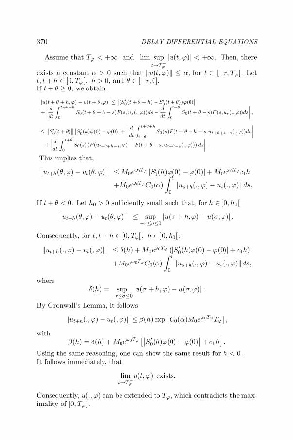
DELAY DIFFERENTIAL EQUATIONS
Assume that Tϕ < +∞ and lim supt→T−
ϕ
|u(t, ϕ)| < +∞. Then, there
exists a constant α > 0 such that ‖u(t, ϕ)‖ ≤ α, for t ∈ [−r, Tϕ[. Lett, t + h ∈ [0, Tϕ[ , h > 0, and θ ∈ [−r, 0].If t + θ ≥ 0, we obtain
|u(t + θ + h, ϕ) − u(t + θ, ϕ)| ≤∣∣(S′
0(t + θ + h) − S′0(t + θ))ϕ(0)
∣∣+
∣∣∣∣ d
dt
∫ t+θ+h
0S0(t + θ + h − s)F (s, us(., ϕ))ds − d
dt
∫ t+θ
0S0(t + θ − s)F (s, us(., ϕ))ds
∣∣∣∣ ,
≤∥∥S′
0(t + θ)∥∥ ∣∣S′
0(h)ϕ(0) − ϕ(0)∣∣ +∣∣∣∣ d
dt
∫ t+θ+h
t+θS0(s)F (t + θ + h − s, ut+θ+h−s(., ϕ))ds
∣∣∣∣+
∣∣∣∣ d
dt
∫ t+θ
0S0(s) (F (ut+θ+h−s, ϕ) − F (t + θ − s, ut+θ−s(., ϕ))) ds
∣∣∣∣ .This implies that,
|ut+h(θ, ϕ)− ut(θ, ϕ)| ≤M0eω0Tϕ |S′
0(h)ϕ(0)− ϕ(0)|+ M0eω0Tϕc1h
+M0eω0TϕC0(α)
∫ t
0‖us+h(., ϕ)− us(., ϕ)‖ ds.
If t + θ < 0. Let h0 > 0 sufficiently small such that, for h ∈ ]0, h0[
|ut+h(θ, ϕ)− ut(θ, ϕ)| ≤ sup−r≤σ≤0
|u(σ + h, ϕ)− u(σ, ϕ)| .
Consequently, for t, t + h ∈ [0, Tϕ[ , h ∈ ]0, h0[ ;
‖ut+h(., ϕ)− ut(, ϕ)‖ ≤ δ(h) + M0eω0Tϕ (|S′
0(h)ϕ(0)− ϕ(0)|+ c1h)
+M0eω0TϕC0(α)
∫ t
0‖us+h(., ϕ)− us(., ϕ)‖ ds,
whereδ(h) = sup
−r≤σ≤0|u(σ + h, ϕ)− u(σ, ϕ)| .
By Gronwall’s Lemma, it follows
‖ut+h(., ϕ)− ut(, ϕ)‖ ≤ β(h) exp[C0(α)M0e
ω0TϕTϕ
],
withβ(h) = δ(h) + M0e
ω0Tϕ[∣∣S′
0(h)ϕ(0)− ϕ(0)∣∣+ c1h
].
Using the same reasoning, one can show the same result for h < 0.It follows immediately, that
limt→T−
ϕ
u(t, ϕ) exists.
Consequently, u(., ϕ) can be extended to Tϕ, which contradicts the max-imality of [0, Tϕ[ .
370

Basic theory of abstract DFE with non-dense domain
We will prove now that the solution depends continuously on theinitial data. Let ϕ ∈ CX , ϕ(0) ∈ D(A0) and t ∈ [0, Tϕ[. We put
α = 1 + sup−r≤s≤t
|u(s, ϕ)|
andc(t) = M0e
ω0t exp(M0e
ω0tC0(α)t).
Let ε ∈ ]0, 1[ such that c(t)ε < 1 and ψ ∈ CX , ψ(0) ∈ D(A0) such that
‖ϕ− ψ‖ < ε.
We have‖ψ‖ ≤ ‖ϕ‖+ ε < α.
LetT0 = sup s > 0 : ‖uσ(., ψ)‖ ≤ α for σ ∈ [0, s] .
If we suppose that T0 < t, we obtain for s ∈ [0, T0] ,
‖us(., ϕ) − us(., ψ)‖ ≤ M0eω0t ‖ϕ − ψ‖ + M0eω0tC0(α)
∫ s
0‖uσ(., ϕ) − uσ(., ψ)‖ dσ.
By Gronwall’s Lemma, we deduce that
‖us(, ϕ)− us(, ψ)‖ ≤ c(t) ‖ϕ− ψ‖ . (3.6)
This implies that
‖us(., ψ)‖ ≤ c(t)ε + α− 1 < α, for all s ∈ [0, T0] .
It follows that T0 cannot be the largest number s > 0 such that ‖uσ(., ψ)‖ ≤α, for σ ∈ [0, s] . Thus, T0 ≥ t and t < Tψ. Furthermore, ‖us(., ψ)‖ ≤ α,for s ∈ [0, t], then using the inequality (3.6) we deduce the dependencecontinuous with the initial data. This completes the proof of Theorem
Theorem 13 Assume that F is continuously differentiable and satisfiesthe following locally Lipschitz condition: for each α > 0 there exists aconstant C1(α) > 0 such that if ϕ1, ϕ2 ∈ CX and ‖ϕ1‖ , ‖ϕ2‖ ≤ α then
|F (t, ϕ1)− F (t, ϕ2)| ≤ C1(α) ‖ϕ1 − ϕ2‖ ,|DtF (t, ϕ1)−DtF (t, ϕ2)| ≤ C1(α) ‖ϕ1 − ϕ2‖ ,|DϕF (t, ϕ1)−DϕF (t, ϕ2)| ≤ C1(α) ‖ϕ1 − ϕ2‖ .
Then, for given ϕ ∈ C1X := C1 ([−r, 0] , X) such that
ϕ(0) ∈ D(A0), ϕ′(0) ∈ D(A0) and ϕ′(0) = Aϕ(0) + F (ϕ),
let u(., ϕ) : [−r, Tϕ[ → X be the unique integral solution of Equation( 1.1). Then, u(., ϕ) is continuously differentiable on [−r, Tϕ[ and satis-fies Equation ( 1.1).
Proof. The proof is similar to the proof of Theorem 10
371

DELAY DIFFERENTIAL EQUATIONS
4. The semigroup and the integrated semigroupin the autonomous case
Let E be defined by
E := D(A)CX =
ϕ ∈ CX : ϕ(0) ∈ D(A0)
.
Throughout this section we will suppose the hypothesis of Theorem 5except that we require F to be autonomous, that is, F : CX → X. Byvirtue of Theorem 5, there exists for each ϕ ∈ E a unique continuousfunction y(., ϕ) : [0, +∞) → X satisfying the following equation
y(t) = S′(t)ϕ +d
dt
∫ t
0S(t− s)X0F (y(s)) ds, for t ≥ 0. (4.1)
Let us consider the operator T (t) : E → E defined, for t ≥ 0 and ϕ ∈ E,by
T (t)(ϕ) = y(t, ϕ).
Then, we have the following result.
Proposition 50 Under the same assumptions as in Theorem 5, thefamily (T (t))t≥0 is a nonlinear strongly continuous semigroup of contin-uous operators on E, that isi) T (0) = Id,ii) T (t + s) = T (t)T (s), for all t, s ≥ 0,iii) for all ϕ ∈ E, T (t)(ϕ) is a continuous function of t ≥ 0 with valuesin E,iv) for all t ≥ 0, T (t) is continuous from E into E.Moreover,v) (T (t))t≥0 satisfies, for t ≥ 0, θ ∈ [−r, 0] and ϕ ∈ E, the translationproperty
(T (t)(ϕ))(θ) =
(T (t + θ)(ϕ))(0), if t + θ ≥ 0,ϕ(t + θ), if t + θ ≤ 0,
(4.2)
andvi) there exists γ > 0 and M ≥ 0 such that,
‖T (t)(ϕ1)− T (t)(ϕ2)‖ ≤ Meγt ‖ϕ1 − ϕ2‖ , for all ϕ1, ϕ2 ∈ E.
Proof. The proof of this proposition is standard.We recall the following definition.
Definition 48 A C0−semigroup (T (t))t≥0 on a Banach space (X, |·|) iscalled compact if all operators T (t) are compact on X for t > 0.
372

Basic theory of abstract DFE with non-dense domain
Lemma 49 Let (S(t))t≥0 a locally Lipschitz continuous integrated semi-group on a Banach space (X, |·|), (A, D(A)) its generator, B a boundedsubset of X, Gλ, λ ∈ Λ a set of continuous functions from the finiteinterval [0, T ] into B, c > 0 a constant and
Pλ(t) =d
dt
∫ t−c
0S(t− s)Gλ(s) ds, for c < t ≤ T + c and λ ∈ Λ.
Assume that S′(t) : (D(A), |·|) → (D(A), |·|) is compact for each t > 0.Then, for each t ∈ (c, T + c], Pλ(t), λ ∈ Λ is a precompact subset of(D(A), |·|).
Proof. The proof is similar to the proof of a fundamental result ofTravis and Webb [94]. Let H = S′(t)x; t ∈ [c, T + c] , x ∈ D(A), |x|≤ kN, where k is the Lipschitz constant of S(·) on [0, T ] and N is abound of B. Using the same reasoning as in the proof of Lemma 2.5 [94],one can prove that H is precompact in (D(A), |·|). Hence, the convexhull of H is precompact. On the other hand, we have, from Lemma 2
Pλ(t) = limh0
1h
∫ t−c
0S′(t− s)S(h)Gλ(s) ds,
and, for each h > 0 small enough and t ∈ (c, T + c] fixed, the set
S′(s)1h
S(h)Gλ(t− s), s ∈ [c, t] , λ ∈ Λ
is contained in H. Then, the set
1h
∫ t
cS′(s)S(h)Gλ(t− s) ds, λ ∈ Λ
is contained in the closed convex hull of (t−c)H. Letting h tend to zero,the set
Pλ(t), λ ∈ Λis still a precompact set of D(A). Hence the proof is complete
Theorem 14 Assume that S′0(t) : (D(A0), |·|) → (D(A0), |·|) is compact
for each t > 0 and the assumptions of Theorem 5 are satisfied. Then, thenonlinear semigroup (T (t))t≥0 is compact on (E, ‖.‖CX
) for every t > r.
Proof. Let ϕλ, λ ∈ Λ be a bounded subset of E and let t > r. Forθ ∈ [−r, 0], we have t + θ > 0. For each λ ∈ Λ, define yλ by
yλ(t)(θ) = y(t, ϕλ)(θ).
373

DELAY DIFFERENTIAL EQUATIONS
Then, we obtain
yλ(t)(θ) = S′0(t + θ)ϕλ(0) + d
dt
∫ t+θ0 S0(t + θ − s)F (yλ(s)) ds,
= S′0(t + θ)ϕλ(0) + lim
h0
1h
∫ t+θ
0S′
0(t + θ − s)S0(h)F (yλ(s)) ds.
First, we show that the family yλ(t), λ ∈ Λ is equicontinuous, for eacht > r. Using the Lipschitz condition on F , one shows thatF (yλ(s)), s ∈ [0, t] and λ ∈ Λ is bounded by a constant, say K.
Let λ ∈ Λ, 0 < c < t− r and −r ≤ θ < θ ≤ 0. Observe that∣∣∣yλ(t)(θ) − yλ(t)(θ)
∣∣∣ ≤∣∣∣S′
0(t + θ)ϕλ(0) − S′0(t + θ)ϕλ(0)
∣∣∣+ lim
h0
1
h
∣∣∣∣∣∫ t+θ
t+θS′
0(t + θ − s)S0(h)F (yλ(s)) ds
∣∣∣∣∣+ lim
h0
1
h
∣∣∣∣∣∫ t+θ
t+θ−c
(S′
0(t + θ − s) − S′0(t + θ − s)
)S0(h)F (yλ(s)) ds
∣∣∣∣∣+ lim
h0
1
h
∣∣∣∣∣∫ t+θ−c
0
(S′
0(t + θ − s) − S′0(t + θ − s)
)S0(h)F (yλ(s)) ds
∣∣∣∣∣ ,
≤∥∥∥S′
0(t + θ)− S′0(t + θ)
∥∥∥ |ϕλ(0)|+ M0eω0tkK
∣∣∣θ − θ∣∣∣+ c2M0e
ω0tkK
+ t sups∈[0,t+θ−c]
∥∥∥S′0(t + θ − s)− S′
0(t + θ − s)∥∥∥ kK.
If we take∣∣∣θ − θ
∣∣∣ small enough, it follows from the uniform continuity
of S′0(.) : [a, t] → L(D(A0)) for 0 < a < t, the claimed equicontinuity of
yλ(t), λ ∈ Λ.On the other hand, the family S′
0(t + θ)ϕλ(0); λ ∈ Λ is precompact,for each t > r and θ ∈ [−r, 0]. We will show that, for each t > r andθ ∈ [−r, 0].
d
dt
∫ t+θ
0S0(t + θ − s)F (yλ(s)) ds; λ ∈ Λ
is precompact.Observe that for 0 < c < t + θ and λ ∈ Λ
1h
∣∣∣∣∫ t+θ
t+θ−cS′
0(t + θ − s)S0(h)F (yλ(s)) ds
∣∣∣∣ ≤ cM0eω0tkK.
Then, if h tends to zero we obtain∣∣∣∣ ddt
∫ t+θ
t+θ−cS0(t + θ − s)F (yλ(s)) ds
∣∣∣∣ ≤ cM0eω0tkK. (4.3)
374

Basic theory of abstract DFE with non-dense domain
For 0 < c < t + θ and λ ∈ Λ,∫ t+θ−c
0S0(t + θ − s)F (yλ(s)) ds =
∫ t+θ
cS0(s)F (yλ(t + θ − s)) ds.
By Lemma 49, if 0 < c < t + θ and λ ∈ Λ, then
d
dt
∫ t+θ−c
0S0(t + θ − s)F (yλ(s)) ds, λ ∈ Λ
is precompact in X, for each t > r and θ ∈ [−r, 0]. This fact togetherwith (4.3) yields the precompactness of the set
d
dt
∫ t+θ
0S0(t + θ − s)F (yλ(s)) ds, λ ∈ Λ
.
Using the Arzela-Ascoli theorem, we obtain the result of Theorem 14Consider now the linear autonomous functional differential equation
u′(t) = A0u(t) + L(ut), t ≥ 0,u0 = ϕ,
(4.4)
where L is a continuous linear functional from CX into X.Given ϕ ∈ CX . It is clear that there exists a unique function
z := z(., ϕ) : [0, +∞) → CX which solves the following abstract integralequation
z(t) = S(t)ϕ +d
dt
(∫ t
0S(t− s)X0L(z(s)) ds
), for t ≥ 0. (4.5)
Theorem 15 The family of operators (U(t))t≥0 defined on CX by
U(t)ϕ = z(t, ϕ),
is a locally Lipschitz continuous integrated semigroup on CX generatedby the operator P defined by
D(P) =ϕ ∈ C1 ([−r, 0] , X) ; ϕ(0) ∈ D(A0),
ϕ′(0) = A0ϕ(0) + L (ϕ) ,Pϕ = ϕ′.
Proof. Consider the operator
L : CX → CX
defined byL (ϕ) = X0L(ϕ).
375

DELAY DIFFERENTIAL EQUATIONS
Using a result of Kellermann [80], one can prove that the operator G
defined in CX by D(G) = D(A),G = A + L,
where A is defined in Proposition 49, is the generator of a locally Lip-schitz continuous integrated semigroup on CX , because A satisfies (HY)and L ∈ L(CX , CX).
Let us introduce the part G of G in CX , which is defined by :
D(G) =
ϕ ∈ D(G); Gϕ ∈ CX
,
G (ϕ) = G (ϕ) .
It is easy to see thatG = P.
Then, P is the generator of a locally Lipschitz continuous integratedsemigroup (V (t))t≥0 on CX .
On the other hand, if we consider, for each ϕ ∈ CX , the nonhomoge-neous Cauchy problem
dz
dt(t) = Az(t) + h(t), for t ≥ 0,
z(0) = 0,(4.6)
where h : [0, +∞[→ CX is given by
h(t) = ϕ + L(V (t)ϕ).
By Theorem 4, the nonhomogeneous Cauchy problem (4.6) has a uniqueintegral solution z given by
z(t) =d
dt
(∫ t
0S(t− s)h(s) ds
),
=d
dt
(∫ t
0S(t− s)ϕ ds
)+
d
dt
(∫ t
0S(t− s)X0L (V (s)ϕ) ds
).
Then,
z(t) = S(t)ϕ +d
dt
(∫ t
0S(t− s)X0L (V (s)ϕ) ds
).
On the other hand, Proposition 47 gives
V (t)ϕ = P(∫ t
0V (s)ϕ ds
)+ tϕ.
376

Basic theory of abstract DFE with non-dense domain
Moreover, for ψ ∈ D(P), we have
Pψ = Aψ + X0L (ψ) .
Then, we obtain
V (t)ϕ = A
(∫ t
0V (s)ϕ ds
)+ X0L
(∫ t
0V (s)ϕ ds
)+ tϕ.
So,
V (t)ϕ = A
(∫ t
0V (s)ϕ ds
)+∫ t
0h(s) ds.
Hence, the function t → V (t)ϕ is an integral solution of Equation (4.6).By uniqueness, we conclude that V (t)ϕ = z(t), for all t ≥ 0. Then wehave U(t) = V (t) on CX . Thus the proof of Theorem 15
Let B be the part of the operator P on E. Then,
D(B) =
ϕ ∈ C1 ([−r, 0] , X) ; ϕ(0) ∈ D(A0), ϕ′(0) ∈ D(A0)ϕ′(0) = A0ϕ(0) + L (ϕ) ,
Bϕ = ϕ′.
Corollary 16 B is the infinitesimal generator of the C0−semigroup(U ′(t))t≥0 on E.
Proof. See [93]
Corollary 17 Under the same assumptions as in Theorem 14, the lin-ear C0−semigroup (U ′(t))t≥0 is compact on E, for every t > r.
To define a fundamental integral solution Z(t) associated to Equation(4.4), we consider, for ϕ ∈ CX , the integral equation
z(t) = S(t)ϕ +d
dt
(∫ t
0S(t− s)X0L(z(s)) ds
), for t ≥ 0. (4.7)
One can show the following result.
Proposition 51 Given ϕ ∈ CX , the abstract integral equation ( 4.7)has a unique solution z := z(., ϕ) which is a continuous mapping from[0, +∞) → CX . Moreover, the family of operators
(U(t)
)t≥0
defined on
CX byU(t)ϕ = z(t, ϕ)
377

DELAY DIFFERENTIAL EQUATIONS
is a locally Lipschitz continuous integrated semigroup on CX generatedby the operator G defined by
D(G) = D(A),Gϕ = A + X0L(ϕ).
For each complex number λ, we define the linear operator
∆(λ) : D(A0) → X
by∆(λ)x := λx−A0x− L
(eλ·x
), x ∈ D(A0).
where eλ·x : [−r, 0]→ CX , is defined for x ∈ X by (note that we considerhere the comlexification of CX)
(eλ·x
)(θ) = eλθx, θ ∈ [−r, 0] .
We will call λ a characteristic value of Equation (4.4) if there existsx ∈ D(A0)\0 solving the characteristic equation ∆(λ)x = 0. Themultiplicity of a characteristic value λ of Equation (4.4) is defined asdim Ker∆(λ).
We have the following result.
Corollary 18 There exits ω ∈ IR, such that for λ > ω and c ∈ X, onehas
(λI − G)−1(X0c) = eλ·∆(λ)−1c.
Proof. We have, for λ > ω0
∆(λ) = (λI −A0)(I − (λI −A0)
−1 L(eλ·I))
.
Let ω > max(0, ω0 + M0 ‖L‖) and
Kλ = (λI −A0)−1 L(eλ·I).
Then,
‖Kλ‖ ≤M0 ‖L‖λ− ω0
< 1, for λ > ω.
Hence the operator ∆(λ) is invertible for λ > ω.Consider the equation
(λI − G)(eλ·a) = X0c,
where c ∈ X is given and we are looking for a ∈ D(A0). This yields
378

Basic theory of abstract DFE with non-dense domain
λeλ·c− λeλ·c + X0
(λc−A0c− L
(eλ·c))
= X0a.
Then, for λ > ωc = ∆(λ)−1a.
Consequently,(λI − G
)−1(X0c) = eλ·∆(λ)−1c
Corollary 19 For each c ∈ X, the function U(.)(X0c) satisfies, fort ≥ 0 and θ ∈ [−r, 0], the following translation property
(U(t)(X0c)
)(θ) =
(U(t + θ)(X0c)
)(0), t + θ ≥ 0,
0, t + θ ≤ 0.
We can consider the following linear operator
Z(t) : X → X
defined, for t ≥ 0 and c ∈ X, by
Z(t)c = U(t)(X0c)(0)
Corollary 20 Z(t) is the fundamental integral solution of Equation( 4.4); that is
∆(λ)−1 = λ
∫ +∞
0e−λtZ(t) dt, for λ > ω.
Proof. We have, for c ∈ X
(λI − G
)−1(X0c) = eλ·∆(λ)−1c.
Then
eλθ∆(λ)−1c = λ
∫ +∞
0e−λs
(U(s)(X0c)
)(θ) ds = λ
∫ +∞
−θe−λsZ(s+θ)c ds.
So,
∆(λ)−1c = λ
∫ +∞
0e−λtZ(t)c dt
It is easy to prove the following result.
Corollary 21 If c ∈ D(A0) then the function
t → Z(t)c
379

DELAY DIFFERENTIAL EQUATIONS
is differentiable for all t > 0 and we have
∆(λ)−1c =∫ +∞
0e−λtZ ′(t)c dt.
Hence the name of fundamental integral solution.
The fundamental solution Z ′(t) is defined only for c ∈ D(A0) and isdiscontinuous at zero. For these reasons we use the fundamental integralsolution Z(t) or equivalently U(.)(X0).
We construct now a variation-of-constants formula for the linear non-homogeneous system
u′(t) = A0u(t) + L(ut) + f(t), t ≥ 0, (4.8)
or its integrated form
y(t) = S′(t)ϕ +d
dt
(∫ t
0S(t− s)X0L [(y(s)) + f(s)] ds
), for t ≥ 0,
(4.9)where f : [0, +∞)→ X is a continuous function.
Theorem 22 For any ϕ ∈ CX , such that ϕ(0) ∈ D(A0), the functiony : [0, +∞) → X defined by
y(t) = U ′(t)ϕ +d
dt
∫ t
0U(t− s)X0f(s) ds, (4.10)
satisfies Equation ( 4.9).
Proof. It follows immediately from Theorem 5 and Corollary 6 that,for ϕ ∈ CX and ϕ(0) ∈ D(A0), Equation (4.9) has a unique solution ywhich is the integral solution of the equation
y′(t) = Ay(t) + X0 [L(y(t)) + f(t)] , t ≥ 0,y(0) = ϕ.
On the other hand, D(A) = D(G) and G = A + X0L. Then, y is theintegral solution of the equation
y′(t) = Gy(t) + X0f(t), t ≥ 0,y(0) = ϕ.
Moreover, we have
D(G) = D(P) =
ϕ ∈ CX , ϕ(0) ∈ D(A0)
= E,
380

Basic theory of abstract DFE with non-dense domain
and the part of G in CX is the operator P. Then t → U(.)ϕ is differen-tiable in t ≥ 0 and Theorem 4 implies
y(t) = U ′(t)ϕ +d
dt
∫ t
0U(t− s)X0f(s) ds
5. Principle of linearized stabilityIn this section, we give a result of linearized stability near an equilib-
rium point of Equation (1.1) in the autonomous case, that is
du
dt(t) = A0u(t) + F (ut), t ≥ 0,
u0 = ϕ.(5.1)
We make the following hypothesis :F is continuously differentiable, F (0) = 0 and F is satisfies the Lipschitzcondition
|F (ϕ1)− F (ϕ2)| ≤ L ‖ϕ1 − ϕ2‖ , for all ϕ1, ϕ2 ∈ CX ,
where L is a positive constant.Let T (t) : E → E, for t ≥ 0, be defined by
T (t)(ϕ) = ut(., ϕ),
where u(., ϕ) is the unique integral solution of Equation (5.1) and
E =
ϕ ∈ CX , ϕ(0) ∈ D(A0)
.
We know that the family (T (t))t≥0 is a nonlinear strongly continuoussemigroups of continuous operators on E.
Consider the linearized equation of (5.1) corresponding to the Frechet-derivative DϕF (0) = F ′(0) at 0 :
du
dt(t) = A0u(t) + F ′(0)ut, t ≥ 0,
u0 = ϕ ∈ CX ,(5.2)
and let (U ′(t))t≥0 be the corresponding linear C0−semigroup on E.
Proposition 52 The Frechet-derivative at zero of the nonlinear semi-group T (t), t ≥ 0, associated to Equation ( 5.1), is the linear semigroupU ′(t), t ≥ 0, associated to Equation ( 5.2).
Proof. It suffices to show that, for each ε > 0, there exists δ > 0such that ∥∥T (t)(ϕ)− U ′(t)ϕ
∥∥ ≤ ε ‖ϕ‖ , for ‖ϕ‖ ≤ δ.
381

DELAY DIFFERENTIAL EQUATIONS
We have
‖T (t)(ϕ)− U ′(t)ϕ‖ = supθ∈[−r,0]
∣∣(T (t)(ϕ)) (θ)−(U ′(t)ϕ
)(θ)∣∣ ,
= supt+θ≥0θ∈[−r,0]
∣∣(T (t)(ϕ)) (θ)−(U ′(t)ϕ
)(θ)∣∣ ,
and, for t + θ ≥ 0
(T (t)(ϕ)) (θ)−(U ′(t)ϕ
)(θ) =
d
dt
∫ t+θ
0S0(t+θ−s)
(F (T (s)(ϕ)) − F ′(0)(U ′(s)ϕ)
)ds.
It follows that
∥∥T (t)(ϕ)− U ′(t)ϕ∥∥ ≤M0e
ω0t
∫ t
0e−ω0s
∣∣F (T (s)(ϕ))− F ′(0)(U ′(s)ϕ)∣∣ ds
and
‖T (t)(ϕ)− U ′(t)ϕ‖ ≤ M0eω0t
(∫ t
0e−ω0s
∣∣F (T (s)(ϕ))− F (U ′(s)ϕ))∣∣ ds
+∫ t
0e−ω0s
∣∣F (U ′(s)ϕ)− F ′(0)(U ′(s)ϕ)∣∣ ds
).
By virtue of the continuous differentiability of F at 0, we deduce thatfor ε > 0, there exists δ > 0 such that∫ t
0e−ω0s
∣∣F (U ′(s)ϕ)− F ′(0)(U ′(s)ϕ)∣∣ ds ≤ ε ‖ϕ‖ , for ‖ϕ‖ ≤ δ.
On the other hand, we obtain∫ t
0e−ω0s ∣∣F (T (s)(ϕ)) − F (U ′(s)ϕ)
∣∣ ds ≤ L
∫ t
0e−ω0s ∥∥T (s)(ϕ) − U ′(s)ϕ
∥∥ ds.
Consequently,
∥∥T (t)(ϕ) − U ′(t)ϕ∥∥ ≤ M0eω0t
(ε ‖ϕ‖ + L
∫ t
0e−ω0s ∥∥T (s)(ϕ) − U ′(s)ϕ
∥∥ ds
).
By Gronwall’s Lemma, we obtain∥∥T (t)(ϕ)− U ′(t)ϕ
∥∥ ≤ M0ε ‖ϕ‖ e(LM0+ω0)t.
We conclude that T (t) is differentiable at 0 and DϕT (t)(0) = U ′(t), foreach t ≥ 0
Definition 49 Let Y be a Banach space, (V (t))t≥0 a strongly continu-ous semigroup of operators V (t) : W ⊆ Y → W, t ≥ 0, and x0 ∈ W
382

Basic theory of abstract DFE with non-dense domain
an equilibrium of (V (t))t≥0 (i.e., V (t)x0 = x0, for all t ≥ 0). Theequilibrium x0 is called exponentially asymptotically stable if there ex-ist δ > 0, µ > 0, k ≥ 1 such that
‖V (t)x − x0‖ ≤ ke−µt ‖x − x0‖ for all x ∈ W with ‖x − x0‖ ≤ δ and all t ≥ 0.
We have the following result.
Theorem 23 Suppose that the zero equilibrium of (U ′(t))t≥0 is expo-nentially asymptotically stable, then zero is exponentially asymptoticallystable equilibrium of (T (t))t≥0 .
The proof of this theorem is based on the following result.
Theorem 24 (Desh and Schappacher [65]) Let (V (t))t≥0 be a nonlinearstrongly continuous semigroup of type γ on a subset W of a Banach spaceY , i.e.
‖V (t)x1 − V (t)x2‖ ≤ M ′eγt ‖x1 − x2‖ , for all x1, x2 ∈ W
and assume that x0 ∈ W is an equilibrium of (V (t))t≥0 such that V (t)is Frechet-differentiable at x0 for each t ≥ 0, with Y (t) the Frechet-derivative at x0 of V (t), t ≥ 0. Then, (Y (t))t≥0 is a strongly continuoussemigroup of bounded linear operators on Y. If the zero equilibrium of(Y (t))t≥0 is exponentially asymptotically stable, then x0 is an exponen-tially asymptotically stable equilibrium of (V (t))t≥0.
6. Spectral DecompositionIn this part, we show in the linear autonomous case (Equation (4.4)),
the existence of a direct sum decomposition of the state space
E =
ϕ ∈ CX , ϕ(0) ∈ D(A0)
into three subspaces : stable, unstable and center, which are semigroupinvariants. We assume that the semigroup (T0(t))t≥0 on D(A0) is com-pact. It follows from the compactness property of the semigroup U ′(t),for t > r, on E, the following results.
Corollary 25 [89] For each t > r, the spectrum σ(U ′(t)) is a countableset and is compact with the only possible accumulation point 0 and ifµ = 0 ∈ σ(U ′(t)) then µ ∈ Pσ(U ′(t)), (where Pσ(U ′(t)) denotes thepoint spectrum).
383

DELAY DIFFERENTIAL EQUATIONS
Corollary 26 [89] There exists a real number δ such that eλ ≤ δ forall λ ∈ σ(B). Moreover, if β is a given real number then there exists onlya finite number of λ ∈ Pσ(B) such that eλ > β.
We can give now an exponential estimate for the semigroup solution.
Proposition 53 Assume that δ is a real number such that eλ ≤ δ forall characteristic values of Equation ( 4.4). Then, for γ > 0 there existsa constant k(γ) ≥ 1 such that
∥∥U ′(t)ϕ∥∥ ≤ k(γ)e(δ+γ)t ‖ϕ‖ , for all t ≥ 0, ϕ ∈ E.
Proof. Let ω1 be defined by
ω1 := inf
ω ∈ lR : supt≥0
(e−ωt
∥∥U ′(t)∥∥) < +∞
.
The compactness property of the semigroup (see [84]) implies that
ω1 = s1(B) := sup eλ : λ ∈ Pσ(B) .
On the other hand, if λ ∈ Pσ(B) then there exists ϕ = 0 ∈ D(B) suchthat Bϕ = λϕ. This implies that
ϕ(θ) = eλtϕ(0) and ϕ′(0) = A0ϕ(0)− L(ϕ) with ϕ(0) = 0.
Then, ∆(λ)ϕ(0) = 0. We deduce that λ is a characteristic value ofEquation (4.4).
We will prove now the existence of λ ∈ Pσ(B) such that eλ = s1(B).Let (λn)n be a sequence in Pσ(B) such that eλn → s1(B) as n → +∞.Then, there exists β such that eλn > β for n ≥ n0 with n0 largeenough. From Corollary 26, we deduce that λn : eλn > β is finite.So, the sequence (eλn)n is stationary. Consequently, there exists nsuch that eλn = s1(B). This completes the proof of Proposition 53
The asymptotic behavior of solutions can be now completely obtainedby the characteristic equation.
Theorem 27 Let δ be the smallest real number such that if λ is a char-acteristic value of Equation ( 4.4), then eλ ≤ δ. If δ < 0, then for allϕ ∈ E, ‖U ′(t)ϕ‖ → 0 as t → +∞. If δ = 0 then there exists ϕ ∈ E\0such that ‖U ′(t)ϕ‖ = ‖ϕ‖ for all t ≥ 0. If δ > 0, then there exists ϕ ∈ Esuch that ‖U ′(t)ϕ‖ → +∞ as t → +∞.
Proof. Assume that δ < 0, then we have ω1 = s1(B) < 0 and thestability holds. If δ = 0, then there exists x = 0 and a complex λ such
384

Basic theory of abstract DFE with non-dense domain
that eλ = 0 and ∆(λ)x = 0. Then, λ ∈ Pσ(B) and eλt ∈ Pσ(U ′(t)).Consequently, there exists ϕ = 0 such that
U ′(t)ϕ = eλtϕ.
This implies that ‖U ′(t)ϕ‖ =∥∥eλtϕ
∥∥ = ‖ϕ‖ . Assume now that δ > 0.Then, there exists x = 0 and a complex λ such that eλ = δ and∆(λ)x = 0. Then, there exists ϕ = 0 such that ‖U ′(t)ϕ‖ = eδt ‖ϕ‖ →+∞, as t → +∞. This completes the proof of Theorem 27
Using the same argument as in [96], [section 3.3, Theorem 3.1], weobtain the following result.
Theorem 28 Suppose that X is complex. Then, there exist three linearsubspaces of E denoted by S, US and CN , respectively, such that
E = S ⊕ US ⊕ CN
and(i) B(S) ⊂ S, B(US) ⊂ US and B(CN) ⊂ CN ;(ii) US and CN are finite dimensional;(iii) Pσ(B |US) = λ ∈ Pσ(B) : eλ > 0 , Pσ(B |CN ) =λ ∈ Pσ(B) : eλ = 0 ;(iv) U ′(t) (US) ⊂ US, U ′(t) (CN) ⊂ CN, for t ∈ lR, U ′(t) (S) ⊂ S, fort ≥ 0;(v) for any 0 < γ < α := inf |eλ| : λ ∈ Pσ(B) and eλ = 0 , thereexists M = M(γ) > 0 such that
‖U ′(t)PUSϕ‖ ≤Meγt ‖PUSϕ‖ , t ≤ 0,
‖U ′(t)PCNϕ‖ ≤Meγ3t ‖PCNϕ‖ , t ∈ lR,
‖U ′(t)PSϕ‖ ≤Me−γt ‖PSϕ‖ , t ≥ 0,
where PS , PUS and PCN are projections of E into S, US and CN re-spectively. S, US and CN are called stale, unstable and center subspacesof the semigroup (U ′(t))t≥0.
7. Existence of bounded solutionsWe reconsider now the equation (4.8) mentioned in the introduction.
For the convenience of the reader, we restate this equationdu
dt(t) = A0u(t) + L(ut) + f(t), t ≥ 0,
u0 = ϕ ∈ CX ,
and its integrated form
ut = U ′(t)ϕ +d
dt
∫ t
0U(t− s)X0f(s)ds, for t ≥ 0. (7.1)
385

DELAY DIFFERENTIAL EQUATIONS
where f is a continuous function form lR into X.Thanks to Lemma 2, we will use the following integrated form of
Equation (4.8), which is equivalent to (7.1) :
ut = U ′(t)ϕ + limλ→+∞
∫ t
0U ′(t− s)BλX0f(s)ds, for t ≥ 0, (7.2)
where the operator Bλ : 〈X0〉 → CX is defined by
BλX0c = λ(λI − G
)−1(X0c) = λeλ·∆(λ)−1c, c ∈ X.
We need the following definition.
Definition 50 We say that the semigroup (U ′(t))t≥0 is hyperbolic if
σ(B) ∩ ilR = ∅.Theorem 28 implies that, in the hyperbolic case the center subspace
CN is reduced to zero. Thus, we have the following result.
Corollary 29 If the semigroup (U ′(t))t≥0 is hyperbolic, then the spaceE is decomposed as
E = S ⊕ US
and there exist positive constants M and γ such that
‖U ′(t)ϕ‖ ≤ Me−γt ‖ϕ‖ , t ≥ 0, ϕ ∈ S,‖U ′(t)ϕ‖ ≤ Meγt ‖ϕ‖ , t ≤ 0, ϕ ∈ US.
We give now the first main result of this section.
Theorem 30 Assume that the semigroup (U ′(t))t≥0 is hyperbolic. LetB represent B(lR−), B(lR+) or B(lR), the set of bounded continuousfunctions from lR−, lR+ or lR respectively to X. Let π : B → B be aprojection onto the integral solutions of Equation ( 4.4) (for any ϕ ∈ E)which are in B. Then, for any f ∈ B, there is a unique solution Kf ∈ Bof Equation ( 7.2) (for some ϕ ∈ E) such that πKf = 0 and K : B → Bis a continuous linear operator. Moreover,(i) for B = B(lR−), we have
π(B) =x : lR− → X, there exists ϕ ∈ US
such that x(t) = (U ′(t)ϕ) (0), t ≤ 0and
(Kf)t = lims→−∞
limλ→+∞
∫ t
sU ′(t− τ)
(BλX0f(τ)
)Sdτ+
limλ→+∞
∫ t
0U ′(t− τ)
(BλX0f(τ)
)USdτ.
386

Basic theory of abstract DFE with non-dense domain
(ii) For B = B(lR+), we have
π(B) =x : lR+ → X, there exists ϕ ∈ S
such that x(t) = (U ′(t)ϕ) (0), t ≥ 0
and
(Kf)t = limλ→+∞
∫ t
0U ′(t− τ)
(BλX0f(τ)
)Sdτ+
lims→+∞
limλ→+∞
∫ t
sU ′(t− τ)
(BλX0f(τ)
)USdτ.
(iii) For B = B(lR), we have
π(B) = 0
and
(Kf)t = lims→−∞
limλ→+∞
∫ t
sU ′(t− τ)
(BλX0f(τ)
)Sdτ+
lims→+∞
limλ→+∞
∫ t
sU ′(t− τ)
(BλX0f(τ)
)USdτ.
Proof. Theorem 28 implies that the space US is finite dimensionaland U ′(t) (US) ⊆ US. Then,x : lR− → X, there exists ϕ ∈ US such that x(t) = (U ′(t)ϕ) (0), t ≤ 0
⊆ π(B(lR−)). Conversely, let ϕ ∈ S and u(., ϕ) be the integral solutionof Equation (4.4) in S, which is bounded on lR−. Assume that there isa t ∈ (−∞, 0] such that ut(., ϕ) = 0. Then, for any s ∈ (−∞, t), we have
ut(., ϕ) = U ′(t− s)us(., ϕ).
Thanks to Corollary 29 we have
‖ut(., ϕ)‖ ≤Me−γ(t−s) ‖us(., ϕ)‖ , s ≤ t.
Since us(., ϕ) is bounded, we deduce that us(., ϕ) = 0. Therefore,
π(B(lR−)) ⊆x : lR− → X, there exists ϕ ∈ US
such that x(t) = (U ′(t)ϕ) (0), t ≤ 0 .
In the same manner, one can prove the same relations for B(lR+) andB(lR).
Let f ∈ B(lR−) and u = u(., ϕ, f) be a solution of Equation (7.2) inB(lR−), with initial value ϕ ∈ E. Then, the function u can be decom-posed as
ut = uUSt + uS
t ,
387
DELAY DIFFERENTIAL EQUATIONS
where uUSt ∈ US and uS
t ∈ S are given by
uUSt = U ′(t−s)uUS
s + limλ→+∞
∫ t
sU ′(t−τ)
(BλX0f(τ)
)USdτ, for t, s ∈ lR,
(7.3)
uSt = U ′(t− s)uS
s + limλ→+∞
∫ t
sU ′(t− τ)
(BλX0f(τ)
)Sdτ, for s ≤ t ≤ 0,
(7.4)since U ′(t) is defined on US for all t ∈ lR. By Corollary 29, we deducethat
uSt = lim
s→−∞lim
λ→+∞
∫ t
sU ′(t− τ)
(BλX0f(τ)
)Sdτ, for t ≤ 0. (7.5)
By Lemma 1, we get BλX0 = λeλ·∆−1(λ). Thus,∥∥∥∥U ′(t− τ)(BλX0f(τ)
)S∥∥∥∥ ≤Me−γ(t−τ) Mλ
λ− ω1sup
τ∈(−∞,0]‖f(τ)‖ .
Consequently, we get
∥∥uSt
∥∥ ≤ MM
γsup
τ∈(−∞,0]‖f(τ)‖ , t ≤ 0. (7.6)
We have proved that
ut = U ′(t)ϕUS + limλ→+∞
∫ t
0U ′(t− τ)
(BλX0f(τ)
)USdτ+
lims→−∞
limλ→+∞
∫ t
sU ′(t− τ)
(BλX0f(τ)
)Sdτ, for t ≤ 0.
(7.7)We obtain also, for t ≤ 0, the following estimate∥∥∥∥U ′(t)ϕUS + lim
λ→+∞
∫ t
0U ′(t− τ)
(BλX0f(τ)
)USdτ
∥∥∥∥ ≤Meγt
∥∥ϕUS∥∥+ MM
γ supτ∈(−∞,0]
‖f(τ)‖ .(7.8)
Conversely, we can verify that the expression (7.7) is a solution of Equa-tion (7.2) in B(lR−) satisfying the estimates (7.6) and (7.8) for everyϕ ∈ E.
Let u = u(., ϕUS , f) be defined by (7.7) and let K : B(lR−) → B(lR−)be defined by Kf = (I − π) u(., 0, f). We can easily verify that
ut(., ϕUS , 0) = U ′(t)ϕUS ,(I − π) u(., ϕUS , 0) = 0,u(., ϕUS , f) = u(., ϕUS , 0) + u(., 0, f).
388

Basic theory of abstract DFE with non-dense domain
Therefore, K is a continuous linear operator on B(lR−), Kf satisfiesEquation (7.2) for every f ∈ B(lR−), πK = 0 and K is explicitly givenby Theorem 30.
For B(lR+) and B(lR) the proofs are similar. This completes the proofof Theorem 30
We consider now the nonlinear equation
du
dt(t) = A0u(t) + L(ut) + g(t, ut), (7.9)
and its integrated form
ut = U ′(t)ϕ + limλ→+∞
∫ t
0U ′(t− s)BλX0g(s, us)ds, (7.10)
where g is continuous from lR× CX into X. We will assume that(H1) g(t, 0) = 0 for t ∈ lR and there exists a nondecreasing functionα : [0, +∞)→ [0, +∞) with lim
h→0α(h) = 0 and
‖g(t, ϕ1)− g(t, ϕ2)‖ ≤ α(h) ‖ϕ1 − ϕ2‖ forϕ1, ϕ2 ∈ E, ‖ϕ1‖ , ‖ϕ2‖ ≤ hand t ∈ lR.
Proposition 54 Assume that the semigroup (U ′(t))t≥0 is hyperbolic andthe assumption (H1) holds. Then, there exists h > 0 and ε ∈ ]0, h[ suchthat for any ϕ ∈ S with ‖ϕ‖ ≤ ε, Equation ( 7.10) has a unique boundedsolution u : [−r, +∞) → X with ‖ut‖ ≤ h for t ≥ 0 and uS
0 = ϕ.
Proof. Let ϕ ∈ S. By Theorem 30, it suffices to establish the exis-tence of a bounded solution u : [−r, +∞) → X of the following equation
ut = U ′(t)ϕ + limλ→+∞
∫ t
0U ′(t− τ)
(BλX0g(τ, uτ )
)Sdτ+
lims→+∞
limλ→+∞
∫ t
sU ′(t− τ)
(BλX0g(τ, uτ )
)USdτ.
Let (u(n))n∈N be a sequence of continuous functions from [−r, +∞) toX, defined by
u(0)t = U ′(t)ϕ
u(n+1)t = U ′(t)ϕ + lim
λ→+∞
∫ t
0U ′(t− τ)
(BλX0g(τ, u(n)
τ ))S
dτ+
lims→+∞
limλ→+∞
∫ t
sU ′(t− τ)
(BλX0g(τ, u(n)
τ ))US
dτ.
It is clear that(u
(n)0
)S= ϕ. Moreover, we can choose h > 0 and ε ∈ ]0, h[
small enough such that, if ‖ϕ‖ ≤ ε then∥∥∥u(n)
t
∥∥∥ < h for t ≥ 0.
389

DELAY DIFFERENTIAL EQUATIONS
On the other hand, we have∥∥∥u(n+1)
t − u(n)t
∥∥∥ ≤∫ t0 MMe−γ(t−τ)α(h)
∥∥∥u(n)τ − u
(n−1)τ
∥∥∥ dτ+∫ +∞t MMeγ(t−τ)α(h)
∥∥∥u(n)τ − u
(n−1)τ
∥∥∥ dτ.
So, by induction we get
∥∥∥u(n+1)t − u
(n)t
∥∥∥ ≤ 2h
(2MMα(h)
γ
)n
, t ≥ 0.
We choose h > 0 such that
2MMα(h)γ
<12.
Consequently, the limit u := limn→+∞
u(n) exists uniformly on [−r, +∞)
and u is continuous on [−r, +∞). Moreover, ‖ut‖ < h for t ≥ 0 anduS
0 = ϕ.In order to prove that u is a solution of Equation (7.10), we introduce
the following notation
v(t) =∥∥∥∥ut − U ′(t)ϕ− lim
λ→+∞
∫ t
0U ′(t− τ)
(BλX0g(τ, uτ )
)Sdτ
− lims→+∞
limλ→+∞
∫ t
sU ′(t− τ)
(BλX0g(τ, uτ )
)USdτ
∥∥∥∥ .
We obtain
v(t) ≤∥∥∥ut − u
(n+1)t
∥∥∥+
∥∥∥∥ limλ→+∞
∫ t
0U ′(t − τ)
((BλX0g(τ, uτ )
)S−(BλX0g(τ, u
(n)τ )
)S)
dτ
∥∥∥∥+
∥∥∥∥ lims→+∞
limλ→+∞
∫ t
sU ′(t − τ)
((BλX0g(τ, uτ )
)US−(BλX0g(τ, u
(n)τ )
)US)
dτ
∥∥∥∥ .
Moreover, we have
ut − u(n+1)t =
+∞∑k=n+1
(u
(k+1)t − u
(k)t
).
It follows that
v(t) ≤ 2h
[1 +
2MMα(h)γ
] +∞∑k=n+1
(2MMα(h)
γ
)k
.
Consequently, v = 0 on [0, +∞).
390

Basic theory of abstract DFE with non-dense domain
To show the uniqueness suppose that w is also a solution of Equation(7.10) with ‖wt‖ < h for t ≥ 0. Then,
∥∥∥wt − u(n+1)t
∥∥∥ ≤∥∥∥∥ limλ→+∞
∫ t
0
U ′(t − τ)
((BλX0g(τ, wτ )
)S
−(BλX0g(τ, u(n)
τ ))S)
dτ
∥∥∥∥+
∥∥∥∥ lims→+∞
limλ→+∞
∫ t
s
U ′(t − τ)
((BλX0g(τ, wτ )
)US
−(BλX0g(τ, u(n)
τ ))US
)dτ
∥∥∥∥ .
This implies
∥∥∥wt − u(n+1)t
∥∥∥ ≤ 2h
(2MMα(h)
γ
)n
→ 0, as n → +∞.
This proves the uniqueness and completes the proof
8. Existence of periodic or almost periodicsolutions
In this section, we are concerned with the existence of periodic (oralmost periodic) solutions of Equations (7.2) and (7.10).
As a consequence of the existence of a bounded solution we obtainthe following result.
Corollary 31 Assume that the semigroup (U ′(t))t≥0 is hyperbolic. Ifthe function f is ω−periodic, then the bounded solution of Equation ( 7.2)given by Theorem 30 is also ω−periodic.
Proof. Let u be the unique bounded solution of Equation (7.2). Thefunction u(. + ω) is also a bounded solution of Equation (7.2). Theuniqueness property implies that u = u(.+ω). This completes the proofof the corollary
We are concerned now with the existence of almost periodic solutionof Equation (7.2). We first recall a definition.
Definition 51 A function g ∈ B(lR) is said to be almost periodic if andonly if the set
gσ : σ ∈ lR ,
where gσ is defined by gσ(t) = g(t + σ), for t ∈ lR, is relatively compactin B(lR).
Theorem 32 Assume that the semigroup (U ′(t))t≥0 is hyperbolic. Ifthe function f is almost periodic, then the bounded solution of Equation( 7.2) is also almost periodic.
391

DELAY DIFFERENTIAL EQUATIONS
Proof. Let AP (lR) be the Banach space of almost periodic functionsfrom lR to X endowed with the uniform norm topology. Define theoperator Q by
(Qf) (t) = lims→−∞
limλ→+∞
∫ t
sU ′(t− τ)
(BλX0f(τ)
)S(0) dτ
+ lims→+∞
limλ→+∞
∫ t
sU ′(t− τ)
(BλX0f(τ)
)US(0) dτ , for t ∈ lR.
Then, Q is a bounded linear operator from AP (lR) into B(lR). By asample computation, we obtain
(Qf)σ = Q (fσ) , for σ ∈ lR.
By the continuity of the operator Q, we deduce that Q(fσ : σ ∈ lR)is relatively compact in B(lR). This implies that if the function f isalmost periodic, then the bounded solution of Equation (7.2) is alsoalmost periodic. This completes the proof of the theorem.
We are concerned now with the existence of almost periodic solutionsof Equation (7.10). We will assume the followings.(H2) g is almost periodic in t uniformly in any compact set of CX . Thismeans that for each ε > 0 and any compact set K of CX there existslε > 0 such that every interval of length lε contains a number τ with theproperty that
supt∈R,ϕ∈K
‖g(t + τ, ϕ)− g(t, ϕ)‖ < ε.
We know from [63] that if the function g is almost periodic in t uniformlyin any compact set of CX and if v is an almost periodic function, thenthe function t → g(t, vt) is also almost periodic.(H3) ‖g(t, ϕ1)− g(t, ϕ2)‖ ≤ K1 ‖ϕ1 − ϕ2‖ , t ∈ lR, ϕ1, ϕ2 ∈ CX .
We have the following result.
Proposition 55 Assume that the semigroup (U ′(t))t≥0 is hyperbolic and(H2), (H3) hold. Then, if in the assumption (H3) K1 is chosen smallenough, Equation ( 7.10) has a unique almost periodic solution.
Proof. Consider the operator H defined on AP (lR) by
Hv = u,
where u is the unique almost periodic solution of Equation (7.2) withf = g(., v.). We can see that there exists a positive constant K2 suchthat
‖Hv1 −Hv2‖ ≤ K1K2 ‖v1 − v2‖ , v1, v2 ∈ AP (lR).
392

Basic theory of abstract DFE with non-dense domain
If K1 is chosen such that K1K2 < 1, then the map H is a strict contrac-tion in AP (lR). So, H has a unique fixed point in AP (lR). This gives analmost periodic solution of Equation (7.10). This completes the proof ofthe proposition
9. ApplicationsWe now consider the two examples mentioned in the introduction.
For the convenience of the reader, we restate the equations.Example 1
∂u
∂t(t, a) +
∂u
∂a(t, a) = f(t, a, ut(·, a)), t ∈ [0, T ] , a ∈ [0, l] ,
u(t, 0) = 0, t ∈ [0, T ] ,u(θ, a) = ϕ(θ, a), θ ∈ [−r, 0] , a ∈ [0, l] .
(9.1)
where T, l > 0, ϕ ∈ CX := C ([−r, 0] , X) and X = C ([0, l] , IR) .By setting U(t) = u(t, ·), Equation (9.1) reads
V ′(t) = A0V (t) + F (t, Vt), t ∈ [0, T ] ,V (0) = ϕ,
where A0 : D(A0) ⊆ X → X is the linear operator defined by
D(A0) =u ∈ C1 ([0, l] , IR) ; u(0) = 0
,
A0u = −u′,
and F : [0, T ]× CX → X is the function defined by
F (t, ϕ)(a) = f(t, a, ϕ(·, a)), for t ∈ [0, T ] , ϕ ∈ CX and a ∈ [0, l] .
We have D(A0) = u ∈ C([0, l] , IR); u(0) = 0 = X. Moreover,
ρ(A0) = C,∥∥∥(λI −A0)−1∥∥∥ ≤ 1
λ , for λ > 0,
this implies that A0 satisfies (HY) on X (with M0 = 1 and ω0 = 0).We have the following result.
Theorem 33 Assume that F is continuous on [0, T ]×CX and satisfiesa Lipschitz condition
|F (t, ϕ)− F (t, ψ)| ≤ L ‖ϕ− ψ‖ , t ∈ [0, T ] and ϕ, ψ ∈ CX ,
with L ≥ 0 constant. Then, for a given ϕ ∈ CX , such that
ϕ(0, 0) = 0,
393

DELAY DIFFERENTIAL EQUATIONS
there exists a unique function u : [0, T ] → X solution of the followinginitial value problem
u(t, a) =
∫ a0 f(τ − a + t , τ , uτ−a+t(·, τ)) dτ, if a ≤ t,
ϕ(0, a − t) +∫ aa−t f(τ − a + t , τ , uτ−a+t(·, τ)) dτ, if a ≥ t ≥ 0,
ϕ(t, a), if t ≤ 0.
(9.2)
Furthermore, u is the unique integral solution of the partial differentialequation ( 9.1), i.e.(i) u ∈ CX ,
∫ t0 u(s, ·)ds ∈ C1 ([0, l] , IR) and
∫ t0 u(s, 0)ds = 0, for t ∈
[0, T ] ,(ii)
u(t, a) =
ϕ(0, a) +∂
∂a
∫ t
0u(s, a) ds +
∫ t
0f(s, a, ut(·, a) ds, if t ∈ [0, T ] ,
ϕ(t, a), if t ∈ [−r, 0] .
Proof. The assumptions of Theorem 33 imply that ϕ ∈ CX andϕ(0, ·) ∈ D(A0). Consequently, from Theorem 5, we deduce that thereexists a unique function v : [0, T ] → CX which solves the integral equa-tion (3.1). It suffices to calculate each term of the integral equation(3.1).
Let (S0(t))t≥0 be the integrated semigroup on X generated by A0. Inview of the definition of (S0(t))t≥0, we have
((λI −A0)
−1 x)
(a) = λ
∫ +∞
0e−λt(S0(t)x)(a) dt.
On the other hand, solving the equation
(λI −A0) y = x, where λ > 0, y ∈ D(A0) and x ∈ X,
we obtain((λI −A0)
−1 x)
(a) = y(a) =∫ a
0e−λtx(a− t) dt.
Integrating by parts one obtains((λI −A0)
−1 x)
(a) = e−λa
∫ a
0x(t)dt +
∫ a
0e−λt
(∫ a
a−tx(s)ds
)dt.
By uniqueness of Laplace transform, we obtain
(S0(t)x) (a) = ∫ a
0 x(s) ds, if a ≤ t,∫ aa−t x(s) ds, if a ≥ t.
394

Basic theory of abstract DFE with non-dense domain
Using Proposition 48, we obtain
(S(t)ϕ) (θ, a) =
∫ 0θ ϕ(s, a) ds +
∫ a0 ϕ(0, τ) dτ, if a ≤ t + θ,∫ 0
θ ϕ(s, a) ds +∫ aa−t−θ ϕ(0, τ) dτ, if a ≥ t + θ ≥ 0,∫ t+θ
θ ϕ(s, a) ds, if t + θ ≤ 0.
The assumption ϕ(0, 0) = 0 implies that S(·)ϕ ∈ C1 ([0, T ] , CX) and wehave
d
dt(S(t)ϕ) (θ, a) =
0, if a ≤ t + θ,ϕ(0, a− t− θ), if a ≥ t + θ ≥ 0,ϕ(t + θ, a), if t + θ ≤ 0.
Remark that the condition ϕ(0, 0) = 0 is necessary to have S(·)ϕ ∈C1 ([0, T ] , CX).
Let G : [0, T ] → X (T > 0) be a Bochner-integrable function andconsider the function K : [0, T ] → CX defined by
K(t) =∫ t
0S0(t− s)X0G(s) ds.
For a ≤ t + θ, we have
K(t)(θ, a) =∫ t+θ0 (S0 (t + θ − s) G (s)) (a) ds,
=∫ t+θ−a0
(∫ a0 G (s) (τ) dτ
)ds +
∫ t+θt+θ−a
(∫ aa−t−θ+s G (s) (τ) dτ
)ds.
For a ≥ t + θ ≥ 0, we obtain
K(t)(θ, a) =∫ t+θ
0
(∫ a
a−t−θ+sG (s) (τ) dτ
)ds,
and for t + θ ≤ 0, we have K(t)(θ, a) = 0.The derivation of K is easily obtained
dK
dt(t)(θ, a) =
∫ a0 G(τ − a + t + θ)(τ) dτ, a ≤ t + θ,∫ aa−t−θ G(τ − a + t + θ)(τ) dτ, a ≥ t + θ ≥ 0,
0, t + θ ≤ 0.
If we consider the function u : [−r, T ] → X defined by
u(t, ·) =
v(t)(0, ·), if t ≥ 0,ϕ(t, ·), if t ≤ 0.
Corollary 7 implies that ut = v(t). Hence, u is the unique solution of(9.2).
395

DELAY DIFFERENTIAL EQUATIONS
The second part of Theorem 33 follows from Corollary 7
Theorem 34 Assume that F is continuously differentiable and thereexist constants L, β, γ ≥ 0 such that
|F (t, ϕ)− F (t, ψ)| ≤ L ‖ϕ− ψ‖ ,|DtF (t, ϕ)−DtF (t, ψ)| ≤ β ‖ϕ− ψ‖ ,|DϕF (t, ϕ)−DϕF (t, ψ)| ≤ γ ‖ϕ− ψ‖ .
Then, for given ϕ ∈ CX such that
∂ϕ
∂t∈ CX , ϕ(0, ·) ∈ C1 ([0, l] , IR) ,
ϕ(0, 0) =∂ϕ
∂t(0, 0) = 0 and
∂ϕ
∂t(0, a) +
∂ϕ
∂a(0, a) = f(0, a, ϕ(·, a)), for a ∈ [0, l] ,
the solution u of Equation ( 9.2) is continuously differentiable on [0, T ]×[0, l] and is equal to the unique solution of Problem ( 9.1).
Proof. One can use Theorem 10 (all the assumptions of this theoremare satisfied).Example 2
∂u
∂t(t, x) = ∆u(t, x) + f(t, x, ut(·, x)), t ∈ [0, T ] , x ∈ Ω,
u(t, x) = 0, t ∈ [0, T ] , x ∈ ∂Ω,u(θ, x) = ϕ(θ, x), θ ∈ [−r, 0] , x ∈ Ω,
(9.3)where Ω ⊂ IRn is a bounded open set with regular boundary ∂Ω, ∆ isthe Laplace operator in the sense of distributions on Ω and ϕ is a givenfunction on CX := C([−r, 0] , X), with X = C
(Ω, IR
).
Problem (9.3) can be reformulated as an abstract semilinear functionaldifferential equation
V ′(t) = A0V (t) + F (t, Vt), t ∈ [0, T ] ,V (0) = ϕ,
with
D(A0) =u ∈ C
(Ω, IR
); ∆u ∈ C
(Ω, IR
)and u = 0 on ∂Ω
,
A0u = ∆u,
and F : [0, T ]× CX → X is defined by
F (t, ϕ)(x) = f(t, x, ϕ(·, x)) for t ∈ [0, T ] , ϕ ∈ CX and x ∈ Ω.
396

Basic theory of abstract DFE with non-dense domain
We have D(A0) =u ∈ C
(Ω, IR
); u = 0 on ∂Ω
, = X.
Moreover ρ(A0)⊂ (0, +∞)∥∥∥(λI −A0)
−1∥∥∥ ≤ 1
λ , for λ > 0,
this implies that A0 satisfies (HY) on X (with M0 = 1 and ω0 = 0).Using the results of Section 3, we obtain the following theorems (the
all assumptions are satisfied).
Theorem 35 Assume that F is continuous on [0, T ]×CX and satisfiesa Lipschitz condition
|F (t, ϕ)− F (t, ψ)| ≤ L ‖ϕ− ψ‖ , t ∈ [0, T ] and ϕ, ψ ∈ CX ,
with L ≥ 0 constant. Then, for a given ϕ ∈ CX , such that
∆ϕ(0, ·) = 0, on ∂Ω,
there exists a unique integral solution u : [0, T ] → X of the partialdifferential equation ( 9.3), i.e.(i) u ∈ CX , ∆
(∫ t0 u(s, ·)ds
)∈ C(Ω, IR
)and
∫ t0 u(s, ·)ds = 0, on ∂Ω,
(ii)
u(t, x) =
ϕ(0, x) + ∆(∫ t
0 u(s, x) ds)
+∫ t0 f(s, x, ut(·, x) ds,
if t ∈ [0, T ] ,
and x ∈ Ω
ϕ(t, x),if t ∈ [−r, 0] ,
and x ∈ Ω.
Theorem 36 Assume that F is continuously differentiable and thereexist constants L, β, γ ≥ 0 such that
|F (t, ϕ)− F (t, ψ)| ≤ L ‖ϕ− ψ‖ ,|DtF (t, ϕ)−DtF (t, ψ)| ≤ β ‖ϕ− ψ‖ ,|DϕF (t, ϕ)−DϕF (t, ψ)| ≤ γ ‖ϕ− ψ‖ .
Then, for given ϕ ∈ CX such that
∂ϕ
∂t∈ CX , ∆ϕ(0, ·) ∈ C
(Ω, IR
),
ϕ(0, ·) = ∂ϕ∂t (0, ·) = 0 on ∂Ω and
∂ϕ
∂t(0, x) = ∆ϕ(0, x) + f(0, x, ϕ(·, x)), for x ∈ Ω.
There is a unique function x defined on [−r, T ]×Ω, such that x = ϕ on[−r, 0]× Ω and satisfies Equation ( 9.3) on [0, T ]× Ω.
397

References
[1] O. Arino (1992) Some spectral properties for the asymptotic be-havior of semigroups connected to population dynamics. SIAMRev. Vol.34, N.4: 445-476.
[2] O. Arino and M. Kimmel (1987) Asymptotic analysis of a cell cyclemodel based on unequal division. SIAM J. Appl. Math. Vol. 47,N.1: 128-145.
[3] O. Arino and M. Kimmel (1989) Asymptotic behavior of a nonlin-ear functional-integral equation of cell kinetics with unequal divi-sion. J. Math. Biol. 27: 341-354.
[4] O. Arino and M. Kimmel (1991) Asymptotic behaviour of nonlin-ear semigroup describing a model of selective cell growth regula-tion. J. Math. Biol. 29: 289-314.
[5] O. Arino and A. Mortabit (1992) A periodicity result for a non-linear functional integral equation. J. Math. Biol. 30: 437-456.
[6] O. Arino and E. Sanchez (1995) Linear Theory of Abstract Func-tional Differential Equations of Retarded Type. J. Math. Anal.and Appl. 191: 547-571.
[7] O. Arino and E. Sanchez (1996) A variation of constants formulafor an abstract functional differential equation of retarded type.Diff. and Int. Equat. Vol.9, N.6: 1305-1320.
[8] O. Arino and E. Sanchez (1998) An integral equation of cell pop-ulation dynamics formulated as an abstract delay equation. Someconsequences. Math. Models and Methods in Applied Sci. Vol.8,N.4: 713-735.
[9] C. Bernier and A. Manitius (1978) On semigroups in Rn × Lp
corresponding to differential equations with delay. Canad. J. Math.30: 897-914.
401

DELAY DIFFERENTIAL EQUATIONS
[10] F.E. Browder (1961) On the spectral theory of elliptic differentialoperators. Math.Ann. 142: 22-130.
[11] A. Calsina and O. El Idrissi (1999) Asymptotic behaviour of anage-structured population model and optimal maturation age. J.Math. Anal. and Appl. 223: 808-826.
[12] S.N. Chow and J. Mallet-Paret (1977) Integral averaging and bi-furcation. J. Diff. Equat. 26: 112-159.
[13] O. Diekmann, H.J. Heijmans and H.R. Thieme (1984) On the sta-bility of the cell size distribution. J. Math. Biol. 19: 227-248.
[14] J. Diestel and J.J. Uhl (1977) Vector Measures. Am. Math. Soc.Mathematical Surveys N.15.
[15] N. Dunford and J. Schwartz (1958) Linear Operators. Part I: Gen-eral Theory. Interscience.
[16] A. Grabosch (1989) Translation semigroups and their lineariza-tions on spaces of integrable functions. Trans. Amer. Math. Soc.311: 357-390.
[17] A. Grabosch and H.J. Heijmans (1991) Production, developmentand maturation of red blood cells: a mathematical model. Math-ematical Population Dynamics. Lect. Notes in Pure and AppliedMathematics. Vol. 131. Marcel Dekker: 189-210.
[18] A. Grabosch and U. Moustakas (1986) A semigroup approach toretarded differential equations. One-Parameter Semigroups of Pos-itive Operators. R. Nagel Ed. Lect. Notes in Math. 1184 (219-232).Springer-Verlag.
[19] J. Hale (1977) Functional Differential Equations. Springer.
[20] J. Hale and S.M. Verduin Lunel (1993) Introduction to FunctionalDifferential Equations. Springer.
[21] E. Hille (1948) Functional analysis and semigroups. Amer. Math.Soc. Colloq. Pub. XXXI. A.M.S. Providence, RI.
[22] G.S. Jones (1962) The existence of periodic solutions off ′(x) = −αf(x − 1)1 + f(x). J. Math. Anal. and Applications.5: 435-450.
[23] T. Kato (1966) Perturbation Theory for Linear Operators.Springer-Verlag.
400

REFERENCES
[24] M. Kimmel, Z. Darzynkiewicz, O. Arino and F. Traganos (1984)Analysis of a cell cycle model based on unequal division ofmetabolic constituents to daughter cells during cytokinesis. J.Theor. Biol. 110: 637-664.
[25] K. Kunish and W. Schappacher (1981) Variation of Constants For-mula for Partial Differential Equations with Delay. Nonlinear Anal.TMA. 5: 123-142.
[26] K. Kunish and W. Schappacher (1983) Necessary conditions forpartial differential equations with delay to generate C0-semigroups.J. Diff. Equations. 50: 49-79.
[27] A. Manitius (1980) Completeness and F-completeness of eigen-functions associated with retarded functional differential equa-tions. J. Diff. Equations. 35: 1-29.
[28] R. Nagel (Ed.) (1986) One-Parameter Semigroups of Positive Op-erators. Lect. Notes Math. 1184. Springer-Verlag.
[29] S. Nakagiri (1981) On the Fundamental Solution of Delay-Differential Equations in Banach Spaces. J. Diff. Equations. 41:349-368.
[30] S. Nakagiri (1987) Pointwise completeness and degeneracy of func-tional differential equations in Banach spaces I: General time de-lays. J. Math. Anal. Appl. 127: 492-529.
[31] S. Nakagiri (1988) Structural properties of functional differentialequations in Banach spaces. Osaka J. Math. 25: 353-398.
[32] R. Nussbaum (1970) The radius of the essential spectrum. DukeMath. J. 37: 473-478.
[33] A. Pazy (1983) Semigroups of linear operators and applications topartial differential equations. Springer Verlag, N.Y.
[34] A.T. Plant (1977) Nonlinear semigroups of translations in Banachspace generated by functional differential equations. J. Math. Anal.Appl. 60: 67-74.
[35] W. Rudin (1973) Functional Analysis. McGraw-Hill.
[36] E. Sanchez, O. Arino and M. Kimmel (1991) Noncompact semi-groups of operators generated by cell kinetics models. Differentialand Integral Equations. Vol.4, N.6: 1233-1249.
401

DELAY DIFFERENTIAL EQUATIONS
[37] H.H. Schaefer (1971) Topological Vector Spaces. Springer Verlag.
[38] K. Shumacher (1985) On the resolvent of linear nonautonomouspartial differential equations. J. Diff. Equations. 59: 355-387.
[39] A. Taylor (1967) Introduction to Functional Analysis. John Wiley.
[40] C.C. Travis and G.F. Webb (1974) Existence and Stability forPartial Functional Differential Equations. Trans. Amer. Math. Soc.200: 395-418.
[41] H.O. Walther (1975) Existence of a nonconstant periodic solutionof a nonlinear nonautonomous functional differential equation rep-resenting the growth of a single species population. J. Math. Biol.1: 227-240.
[42] G.F. Webb (1985) Theory of Nonlinear Age-Dependent PopulationDynamics. Marcel Dekker Inc.
[43] M.Adimy, Integrated semigroups and delay differential equations,Journal of .Mathematical Analysis and .Applications, 177, (1993),125-134.
[44] M. Adimy et K. Ezzinbi, Semi-groupes integres et equationsdifferentielles a retard en dimension infinie, C. R. Acad. Sci. Paris,t.323, Serie I, (1996), 481-486.
[45] M. Adimy et K. Ezzinbi, Local existence and linearized stabilityfor partial functional differential equations, Dynamic Systems andapplications, 7, (1998), 389-404.
[46] M Adimy and K. Ezzinbi, A class of linear partial neutral func-tional differential equations with non-dense domain, Journal ofDifferential Equations, 147, (1998), 285-332.
[47] M Adimy and K. Ezzinbi, Existence and linearized stability forpartial neutral functional differential equations, Journal of Differ-ential Equations and Dynamical Systems Vol. 7, Number 4, Octo-ber, (1999), 371-417.
[48] M. Adimy and K. Ezzinbi, Some results on existence, asymptoticbehavior and stability of solutions for a class of partial neutralfunctional differential equations, Hiroshima Mathematical Journal,(to appear 2004).
402

REFERENCES
[49] M Adimy, K. Ezzinbi and M. Laklach, Local existence and globalcontinuation for a class of partial neutral functional differentialequations, C.R.Acad. Sci. Paris, t.330, Serie I, (2000), 957-962.
[50] M Adimy, H.Bouzahir and K. Ezzinbi, Existence for a class ofpartial functional differential equations with infinite delay, Journalof Nonlinear Analysis, Theory, Methods and Applications, Vol 46,No. 1, (2001), 91-112.
[51] M Adimy, H. Bouzahir and K. Ezzinbi, Local existence and sta-bility for a class of partial functional differential equations withinfinite delay, Journal of Nonlinear Analysis, Theory, Methods andApplications, 48, (2002), 323-348.
[52] M. Adimy, H. Bouzahir and K. Ezzinbi, Local existence for a classof partial neutral functional differential equations with infinite de-lay, Journal of Differential Equations and Dynamical Systems, (toappear 2004).
[53] M. Adimy, H. Bouzahir and K. Ezzinbi, Existence and stability forsome partial neutral functional differential equations with infinitedelay, Journal of Mathematical Analysis and Applications, Vol.294, Issue 2, (2004), 438-461.
[54] M. Adimy, K.Ezzinbi and M. Laklach, Spectral decompostion forsome neutral partial functional differential equations, CanadianApplied Mathematics Quarterly, Vol. 9, No.4, Winter (2001), 1-34.
[55] E. Ait Dads and K. Ezzinbi, Boundedness and almost peri-odicity for some state-dependent delay differential equations,Electronic Journal of Differential Equations, Vol. 2002, No. 67,http://ejde.math.swt.edu , (2002), 1-13.
[56] W.Arendt, Resolvant positive operators and integrated semigroup,Proc. London Math. Soc., 3, vol.54, (1987), 321-349.
[57] W.Arendt, Vector valued Laplace transforms and Cauchy prob-lems, Israel J.Math., 59, (1987), 327-352.
403

DELAY DIFFERENTIAL EQUATIONS
[58] O.Arino et E.Sanchez, Linear theory of abstract functional differ-ential equations of retarded type, Journal of .Mathematical Analy-sis and Applications, 191, (1995), 547-571.
[59] R. Benkhalti and K. Ezzinbi, Existence and stability for some par-tial neutral functional differential equations, Differential and In-tegral Equations, (to appear 2004).
[60] K. Ezzinbi and R. Benkhalti, Periodic solutions for some partialfunctional differential equations, Journal of Applied Mathematicsand Stochastic Analysis, (to appear 2004).
[61] S.Busenberg and B.Wu, Convergence theorems for integrated semi-group, Diff. Int. Eq. 5, vol. 3, May, (1992), 509-520.
[62] P.Clement, O.Diekmann, M.Gyllenberg, H.J.A.M. Heijmans andH.R.Thieme, Perturbation theory for dual semigroups. I. the sun-reflexive case, Math. Ann., 277, (1987), 709-725.
[63] C. Corduneanu, Almost Periodic Functions, 2nd edition, Chelsea, New York (1989).
[64] G.Da Prato and E.Sinestrari, Differential operators with non-densedomains, Ann., Scuola, Norm.,Sup. Pisa Cl. Sci., 14, (1987), 285-344.
[65] W. Desch and W. Schappacher, Linearized stability for nonlin-ear semigroups, in “Differential Equations in Banach Spaces”(A.Favini and E.Obrecht, Eds.) pp. 61-73, Lecture Notes in Math.,Vol. 1223, Springer-Verlag, New York / Berlin (1986).
[66] O. Diekmann, S. A. Van Gils, S. M. Verduyn Lunel and H. O.Walther, Delay Equations, Functional, Complex and NonlinearAnalysis, Springer-Verlag, (1995).
[67] K. Ezzinbi, Existence and stability for some partial functrional dif-ferential equations with infinite delay, Electronic Journal of Dif-ferential Equations, Vol. 2003, No. 116, http://ejde.math.swt.edu,(2003), 1-13.
[68] K. Ezzinbi and M. Jazar, New criteria for the existence of pe-riodic and almost periodic solutions for some evolution equa-tions in Banach spaces, Electronic Journal of Qualitative The-ory of Differential Equations, No.6, (2004), http://www.math.u-szeged.hu/ejqtde/, 1-12.
404

REFERENCES
[69] K. Ezzinbi and S.L.Rhali, Positivity and stability for some partialfunctional differential equations, Nonlinear Differential Equationsand Applications, Vol. 10, No. 1, (2003), 1-13.
[70] K. Ezzinbi and J. H. Liu, Periodic solutions of Non-Densely defineddelay evolution equations, Journal of Applied Mathematics andStochastic Analysis, , Vol. 15, No. 2, (2002), 113-123.
[71] K.Ezzinbi anf J.H. Liu, Non-densely defined evolution equationswith non local conditions, Mathematical and Computer Modeling,36, (2002), 1027-1038.
[72] W.E.Fitzgibbon, Semilinear functional differential equations inBanach space, J. Differential Equ. 29, (1978), 1-14.
[73] A.Grabosch and U.Moustakas, A semigroup approach to retardeddifferential equations, in ” One-Parameter Semigroups of PositiveOperators (R.Nagel, ed.), p 219-232, Lecture Notes in Mathemat-ics, Vol. 1184, Springer-Verlag, Berlin/New York, (1986).
[74] J.K.Hale, Theory of functional differential equations Springer-Verlag, New York, (1977).
[75] J.K.Hale and S.Lunel, Introduction to functional differential equa-tions, Springer-Verlag, New York (1993).
[76] M.Hieber, Integrated semigroups and diff. operators on Lp, Dis-sertation, (1989).
[77] T.Kato, Perturbation theory for linear operators, Springer, Berlin(1966).
[78] K.Kunish and W.Schappacher, Variation-of-constants formula forpartial differential equations with delay, Nonlinear Anal. TMA 5,(1981), 123-142.
[79] K.Kunish and W.Schappacher, Necessary conditions for partial dif-ferential equations with delay to generate a C0−semigroups, J.D.E50, (1983), 49-79.
[80] H. Kellermann, Integrated Semigroups, Dissertation, Tubingen,(1986).
[81] H.Kellermann and M.Hieber, Integrated semigroup, J.Fun.Anal.,15, (1989), 160-180.
405

DELAY DIFFERENTIAL EQUATIONS
[82] M.Memory, Stable and unstable manifolds for partial functionaldifferential equations, Nonlinear Analysis, Theory, Methods andApplications, 16, (1991), 131-142.
[83] M.Memory, Invariant manifolds for partial functional differentialequations, In Mathematical Population Dynamics (Eds. O.Arino,D.E.Axelrod and M.Kimmel) (1991), 223-232, Marcel-Dekker.
[84] R. Nagel, One-parameter Semigroups of Positive Operators, Lect.Notes in Mathematics, Springer-Verlag, 1184, (1986).
[85] R. Nagel and E. Sinestrari, Nonlinear hyperbolic Volterra integrod-ifferential equations, Nonlinear Anal. TMA, Vol.27, No.2, (1996),167-186.
[86] F.Neubrander, Integrated semigroups and their applications to theabstract Cauchy problems, Pacific, J. Math., 135, (1988), 111-155.
[87] M.E. Parrrot, Positivity and a principle of linearized stability fordelay differential equations, J. Diff. and Integ. Equa., 2, (1989),170-182.
[88] M.E. Parrrot, Linearized stability and irreducibility for a func-tional differential equation, SIAM J. Math. Anal., 23, (1992), 649-661.
[89] A.Pazy, Semigroups of linear operators and applications to partialdifferential equations, Springer, Berlin (1983).
[90] W.M. Ruess and W. H. Summers, Linearized stability for abstractdifferential equations with delay, Journal of Mathematical Analysisand Applications, 198, (1996), 310-336.
[91] E.Sinestrari, On the abstract Cauchy problem of parabolic type inspaces of continuous functions; Journal of .Mathematical .Analysisand .Applications, 107 (1985), 16-66.
[92] H.Thieme, Integrated semigroups and integrated solutions to ab-stract Cauchy problems, Journal of .Mathematical .Analysis and.Applications, 152, (1990), 416-447.
[93] H.Thieme, Semiflows generated by Lipschitz perturbations of non-densely defined operators, Diff. Integr. Equations 3, No.6, (1990),1035-1066.
406

REFERENCES
[94] C.C.Travis and G.F.Webb, Existence and stability for partial func-tional differential equations, Trans. Amer. Math. Soc. 200, (1974),395-418.
[95] G.F.Webb, Asymptotic stability for abstract functional differentialequations, Proc. Amer. Math.Soc. 54 (1976), 225-230.
[96] J. Wu, Theory and Applications of Partial Functional DifferentialEquations, Springer-Verlag, (1996).
407

Chapter 10
DYNAMICS OF DELAY DIFFERENTIALEQUATIONS
H.O. WaltherMathematisches InstitutUniversitat GiessenArndtstr. 2D 35392 [email protected]
1. Basic theory and some results for examplesProofs for most of the basic results presented in this part are found inthe monograph [57]. See also [105].
1.1 Semiflows of retarded functional differentialequations
Let h > 0, n ∈ N. Let C denote the Banach space C([−h, 0], Rn), with‖φ‖ = max−h≤s≤0 |φ(s)|. The space C will serve as state space. For x :R ⊃ I → R
n and t ∈ R with [t− h, t] ⊂ I, the segment xt : [−h, 0]→ Rn
is the shifted restriction of x to the initial interval [−h, 0],
xt(s) = x(t + s) for s ∈ [−h, 0].
Autonomous retarded functional differential equations on C (RFDEs)are equations of the form
x(t) = f(xt),
for a given map f : C ⊃ U → Rn. In the sequel we shall assume that
U ⊂ C is open and that f is locally Lipschitz continuous. Some resultsrequire that f is continuously differentiable. Solutions x : [t0 − h, te) →R
n, −∞ < t0 < te ≤ ∞, of the previous RFDE are continuous, differ-entiable on (t0, te), and satisfy the RFDE for t0 < t < te. This implies
© 2006 Springer.
411
O. Arino et al. (eds.), Delay Differential Equations and Applications, 411–476.

DELAY DIFFERENTIAL EQUATIONS
that their right derivative at t0 exists and equals f(xt0). Solutions on(−∞, te) (including on R) are differentiable and satisfy the RFDE every-where.
A maximal solution xφ : [t0 − h, te(φ)) → Rn of the initial value
problem (IVP)x(t) = f(xt), x0 = φ ∈ U,
is a solution of the RFDE which satisfies the initial condition and hasthe property that any other solution of the same IVP is a restriction ofxφ.
Example. Let µ ∈ R and a continuously differentiable function g :R → R be given. The equation
x(t) = −µx(t) + g(x(t− 1)) (1.1)
is an RFDE, with h = 1, n = 1, and f(φ) = −µφ(0) + g(φ(−1)) for allφ ∈ C. Solutions are easily found via the method of steps: For φ ∈ Cgiven, evaluate successively the variation-of-constants formulae
x(t) = e−µ(t−n)x(n) +∫ t
ne−µ(t−s)f(x(s− 1))ds,
for nonnegative integers n and n ≤ t ≤ n + 1, with x0 = φ. This yieldsthe maximal solution xφ : [−1,∞) → R of the IVP for eq. (1.1). - Ifg(0) = 0 then x : R t → 0 ∈ R is a constant solution (equilibriumsolution). For µ > 0 and
ξ g(ξ) < 0 for all ξ = 0
eq. (1.1) models a combination of delayed negative feedback and in-stantaneous negative feedback with respect to the zero solution. Thecondition
ξ g(ξ) > 0 for all ξ = 0
corresponds to delayed positive (and instantaneous negative) feedback.
In case of negative feedback and µ ≥ 0, initial data with at most onezero define slowly oscillating solutions, which have any two zeros spacedat a distance larger than the delay h = 1.
How is slowly oscillating behaviour reflected in the state space C ? Seg-ments xt of slowly oscillating solutions belong to the set S ⊂ C \ 0 of
412

Dynamics of Delay Differential Equations
Figure 10.1.
Figure 10.2.
initial data with at most one change of sign. More precisely, φ = 0, and0 ≤ φ, or φ ≤ 0, or there are j ∈ 0, 1 and a ∈ [−1, 0] so that
0 ≤ (−1)jφ(t) on [−1, a], (−1)jφ(t) ≤ 0 on [a, 0].
The set S is positively invariant, i.e., for all φ ∈ S and all t ≥ 0, xφt ∈ S.
We havecl S = S ∪ 0,
and(0,∞) · S ⊂ S
which says that S is a wedge. It can be shown that S is homotopyequivalent to the circle; S is not convex. See [240].
Let us call a solution eventually slowly oscillating if for some t its zerosz ≥ t are spaced at distances larger than the delay h = 1. The mainresult of [177] establishes that in case µ ≥ 0, g bounded from below orfrom above, and
g′(ξ) < 0 for all ξ ∈ R
almost every initial function φ ∈ C defines a solution which is eventuallyslowly oscillating. More precisely, the set R of data whose maximal
413

DELAY DIFFERENTIAL EQUATIONS
solutions are not eventually slowly oscillating is closed and a graph
T ⊃ dom→ Q
with respect to a decomposition of C into a closed subspace T of codi-mension 2 and a 2-dimensional complementary subspace Q. This showsthat the set C \R of initial data of eventually slowly oscillating solutionsis open and dense in C.
Remark. For certain bounded but non-monotone functions g and forcertain µ > 0 there exist rapidly oscillating periodic solutions with at-tracting orbits [116]. This means that for such g and µ the previousstatement is false.
Problem. Does the density result hold in case µ = 0 for all g whichsatisfy the negative feedback condition ?
We shall see that in case of negative feedback slowly oscillating pe-riodic solutions play a prominent role in the dynamics generated byeq.(1.1). In a simple case, which was excluded from the considerationsup to here, they are easily found.
Exercises. Define and compute a ‘slowly oscillating periodic solution’of eq. (1.1) for µ = 0 and the step function g = −sign. Then com-pute a slowly oscillating periodic solution for a suitable smooth functiong which is positive and constant on some interval (−∞,−a] and linearand decreasing on some interval [−b,∞), 0 < b < a.
In case of positive feedback, the convex cones of nonnegative and non-positive data are positively invariant. See [137].
Back to the general case. The maximal solutions of the IVP witht0 = 0 define a continuous semiflow
F : Ω → U,
F (t, φ) = xφt
andΩ = (t, φ) ∈ [0,∞)× U : t < te(φ).
The domain Ω is open in [0,∞) × U . Recall the algebraic semiflowproperties
F (0, φ) = φ and
414

Dynamics of Delay Differential Equations
F (t, F (s, φ)) = F (t+s, φ) whenever φ ∈ U, 0 ≤ s < te(φ), 0 ≤ t < te(F (s, φ)).
The solution maps Ft = F (t, ·), t ≥ 0, are defined on the open setsΩt = φ ∈ U : (t, φ) ∈ Ω. For certain t > 0, Ωt may be empty.
Remark. A flow does not exist in general, as there are no backwardsolutions for nondifferentiable initial data. Also, initially different solu-tions may become identical on some ray [t,∞). Therefore solutions ofthe backward IVP are in general not uniquely determined.
Example. Eq. (1.1) with g constant on a nontrivial interval I, initialdata φ = ψ with range in I and φ(0) = ψ(0).
Before discussing differentiability with respect to initial data a lookat nonautonomous linear delay differential equations is convenient: LetL : [t0, te)× C → R
n, t0 < te ≤ ∞, be continuous and assume all mapsL(t, ·) are linear. Solutions of the equation
y(t) = L(t, yt)
are defined as before. Maximal solutions exist and are defined on [t0 −h, te).
Suppose f is continuously differentiable. For a given maximal so-lution x = xφ : [t0 − h, te(φ)) → R
n of an IVP associated with thenonlinear RFDE above the variational equation along x is the previouslinear equation with
L(t, ψ) = Df(xt)ψ for t0 ≤ t < te(φ), ψ ∈ C.
Example. Let g(0) = 0. The variational equation along the zerosolution of eq. (1.1), or linearization at 0, is
v(t) = −µ v(t) + α v(t− 1) (1.2)
with α = g′(0).
In case f is continuously differentiable all solution operators Ft on non-empty domains are continuously differentiable, and for all φ ∈ Ωt, χ ∈ C,
DFt(φ)χ = vφ,χt
with the maximal solution vφ,χ : [−h, te(φ)) → Rn of the IVP
v(s) = Df(F (s, φ))vs, v0 = χ.
415

DELAY DIFFERENTIAL EQUATIONS
On the open subset of Ω given by t > h the semiflow F is continuouslydifferentiable, with
D1F (t, φ)1 = xφt .
I.e., for t > h the tangent vectors of the flowline
[0, te(φ)) t → F (t, φ) ∈ U
exist and are given by the derivatives of the solution segments. Noticethat for 0 ≤ t < h the solution segments are in general only continuousand not differentiable.
1.2 Periodic orbits and Poincare return mapsLet a periodic solution x : R → R
n of the RFDE be given. Assume f iscontinuously differentiable. Let p > h be a period of x, not necessarilyminimal. A transversal to the periodic orbit
o = xt : t ∈ [0, p] ⊂ U
at x0 = xp is a hyperplane H = x0 + L, with a closed subspace L ofcodimension 1, so that
D1F (p, x0)1 /∈ L = Tx0H.
Recall that L is the kernel of a continuous linear functional φ∗. Therelation F (t, φ) ∈ H is equivalent to the equation
φ∗(F (t, φ)− x0) = 0.
An application of the Implicit Function Theorem close to the solution(p, x0) yields an open neighbourhood N of x0 in C and a continuouslydifferentiable intersection map
τ : N → R
so that τ(x0) = p and
F (τ(φ), φ) ∈ H for all φ ∈ N.
The Poincare return map
P : H ∩N φ → F (τ(φ), φ) ∈ H
is continuously differentiable (with respect to the C1-submanifold struc-tures on H ∩N and H).
416

Dynamics of Delay Differential Equations
Figure 10.3.
The derivatives DP (φ)χ, φ ∈ H ∩N and χ ∈ TφH = L, are given by
prφ DFτ(φ)(φ)χ
where prφ : C → L is the projection along the (tangent) vector
η = D1F (τ(φ), φ)1 = xφτ(φ) /∈ L.
We haveprφψ = ψ − φ∗ψ
φ∗ηη.
Figure 10.4.
In particular,DP (x0)χ = prx0DFp(x0)χ.
417

DELAY DIFFERENTIAL EQUATIONS
1.3 CompactnessOften the solution maps Ft, t ≥ h, are compact in the sense that theymap bounded sets into sets with compact closure. (F0 = idU is notcompact, due to dim C = ∞).
Example. Eq. (1.1) with g bounded from above or from below. Com-pactness follows by means of the Ascoli-Arzela Theorem from simplea-priori bounds on solutions and their derivatives.
Also Poincare maps are often compact. It follows that all these mapsare not diffeomorphisms. Therefore standard tools of dynamical systemstheory on finite-dimensional manifolds, which had originally been devel-opped for diffeomorphisms only, e.g., local invariant manifolds, inclina-tion lemmas, and the shadowing lemma associated with a hyperbolic set,had to be generalized in a suitable way for differentiable, not necessarilyinvertible maps in Banach spaces.
1.4 Global attractorsConsider a semiflow F : [0,∞) ×M → M on a complete metric spaceM . A complete flowline is a curve u : R → M so that
F (t, u(s)) = u(t + s) for all t ≥ 0, s ∈ R.
A set I ⊂ M is invariant if each x ∈ I is a value of a complete flowlineu with u(R) ⊂ I. This is equivalent to
Ft(I) = I for all t > 0.
A (compact) global attractor A for F is a compact invariant set A ⊂ Mwhich attracts bounded sets in the sense that for every bounded setB ⊂ M and for every open set V ⊃ A there exists t ≥ 0 such thatF (s, B) ⊂ V for all s ≥ t.
Exercise. A global attractor contains each bounded set B ⊂M whichsatisfies B ⊂ F (t, B) for all t > 0.
It follows from the exercise that a global attractor A contains everycompact invariant set, and that it is uniquely determined. Furthermore,A coincides with the set of all values of all bounded complete flowlines.
Existence of global attractors is in some cases easy to verify. Considerfor example eq. (1) with µ > 0 and g : R → R injective and bounded.
418

Dynamics of Delay Differential Equations
Then all solution maps are injective, and F1 is compact. For r > 1 +(sup |g|)/µ the open ball Cr in C with radius r > 0 and center 0 ispositively invariant under the semiflow and absorbs every flowline in thesense that for every φ ∈ C there exists t ≥ 0 with F (s, φ) ∈ Cr for alls ≥ t. The set
A =⋂t≥0
F (t, Cr)
is the global attractor [137].
1.5 Linear autonomous equations and spectraldecomposition
For L : C → Rn linear continuous, consider the RFDE
y(t) = Lyt.
The semiflow is now given by the C0-semigroup of solution operatorsTt : C φ → yφ
t ∈ C, t ≥ 0. The domain of its generator G : DG → C is
DG = φ ∈ C : φ continuously differentiable, φ(0) = Lφ,
and Gφ = φ. The solution behaviour is determined by the spectrumof the generator. The solution operators are compact for t ≥ h, andthe complexification of G has compact resolvents. So the spectrum σof G consists of a countable number of isolated eigenvalues of finitemultiplicities, which are real or occur in complex conjugate pairs. TheAnsatz y(t) = eλt c for a solution leads to a characteristic equation forthe eigenvalues. Example: For eq. (1.2),
λ + µ− α e−λ = 0.
An important property is that any halfplane given by an equation
Reλ > β
for β ∈ R contains at most a finite number of eigenvalues.
Examples. For eq. (1.2) with µ = 0, α < −π2 (negative feedback),
there exist pairs of complex conjugate eigenvalues with positive real part,and there are no real eigenvalues. In case µ > 0 and α > 0 (positivefeedback) the eigenvalue with largest real part is positive and all othereigenvalues form complex conjugate pairs.
419

DELAY DIFFERENTIAL EQUATIONS
Figure 10.5.
420

Dynamics of Delay Differential Equations
Rapid growth of the imaginary parts of the eigenvalues as Reλ → −∞shows that G is not sectorial, and that the semigroup is not analytic.
The realified generalized eigenspaces associated with a real eigenvalueor a pair of complex conjugate eigenvalues are positively invariant underthe semigroup, as well as generalized eigenspaces C<β associated withall eigenvalues in a left halfplane given by an equation
Reλ < β,
with β ∈ R. On the finite-dimensional generalized eigenspace C≥β givenby the set σ≥β of all eigenvalues satisfying
Reλ ≥ β
the semigroup induces a group of isomorphisms Tt,β = eBt, t ∈ R, with alinear vectorfield B : C≥β → C≥β . The spectrum of B is σ≥β; generalizedeigenspaces of an eigenvalue with respect to G and B coincide. On thecomplementary subspace C<β ,
‖Ttφ‖ ≤ k eβ t‖φ‖, t ≥ 0,
with k = k(L, β) ≥ 0.
The unstable, center, and stable subspaces Cu, Cc, Cs of G are therealified generalized eigenspaces given by the sets σ>0, σ0, σ<0 of theeigenvalues with positive, zero, and negative real part, respectively. Cu
consists of segments of solutions on the line which decay to 0 exponen-tially as t → −∞ and whose segments grow exponentially as t → ∞.Cc consists of segments of solutions with polynomial growth. Solutionsstarting in Cs decay exponentially to 0 as t →∞. We have
C = Cu ⊕ Cc ⊕ Cs.
The semigroup is called hyperbolic is there are no eigenvalues on theimaginary axis.
Examples of other spectral decompositions of C. Consider eq. (1.2).In the case µ ≥ 0 and α < 0 (negative feedback), there is a leading pair ofeigenvalues, i.e., there exists β ∈ R so that the sum of the multiplicitiesof the eigenvalues with Reλ > β is 2. For convenience we choose β sothat there are no eigenvalues on β + iR. For the leading eigenvalues,
|Imλ| < π,
421

DELAY DIFFERENTIAL EQUATIONS
and all solutions with segments in the 2-dimensional space
C2 = C>β
are slowly oscillating. Solutions on the line with segments in realifiedgeneralized eigenspaces associated with other complex conjugate pairsof eigenvalues are not slowly oscillating. Later we shall consider thedecomposition
C = C2 ⊕ C2<
where C2< = C<β . We have
C2 ⊂ S ∪ 0
andS ∩ C2< = ∅.
See [240].
Figure 10.6.
In the result from [177] on density of initial data for eventually slowlyoscillating solutions of the nonlinear eq. (1.2), we actually have T = C2<
and Q = C2, for the space T containing the domain dom of the map rep-resenting the thin set R of segments of rapidly oscillating solutions andfor the target space Q of this map. Of course, C2< and C2 are heredefined by the variational equation (1.2) along the zero solution of eq.(1.1).
422

Dynamics of Delay Differential Equations
In the positive feedback case µ ≥ 0 and α > 0, with α sufficientlylarge, there are at least 3 eigenvalues in the open right halfplane. Chooseβ > 0 so that the 3 eigenvalues with largest real parts satisfy β < Reλ,and there are no eigenvalues on β + iR. The solutions on the line withsegments in
C3 = C>β
have at most 2 zeros in any interval of length h = 1, and they decayto 0 as t → −∞ faster than t → eβ t. Later we shall consider thedecomposition
C = C3 ⊕ C3<
where C3< = C<β . See [137].
Figure 10.7.
1.6 Local invariant manifolds for nonlinearRFDEs
Assume f is continuously differentiable, and f(φ0) = 0. For simplicity,φ0 = 0. Then the zero function on the line is a solution, and 0 ∈ U isa stationary point of the semiflow: F (t, 0) = 0 for all t ≥ 0. The linearvariational equation along the zero solution is given by
L = Df(0).
There exist open neighbourhoods Nu, N c, N s of 0 in the spaces Cu, Cc, Cs,respectively, and continuously differentiable maps
wu : Nu → Cc ⊕ Cs, wc : N c → Cu ⊕ Cs, ws : N s → Cu ⊕ Cc
with fixed point 0 and zero derivatives at 0 whose graphs
W ∗ = χ + w∗(χ) : χ ∈ N∗
423

DELAY DIFFERENTIAL EQUATIONS
are locally positively invariant under the semiflow F . This means thatthere is a neighbourhood N of 0 so that flowlines starting in N ∩W ∗
remain in W ∗ as long as they stay in N . The local unstable manifold W u
consists of segments of solutions x : (−∞, te) → Rn which decay to 0 ex-
ponentially as t → −∞. Conversely, all such solutions with all segmentsin a neighbourhood of 0 in C have their segments in W u. All boundedsolutions on the line which remain sufficiently small have all their seg-ments in W c. All solutions which start in W s decay to 0 exponentially ast →∞, and the segments of all solutions on [−h,∞) which remain in aneighbourhood of 0 and tend to 0 exponentially as t →∞ belong to W s.
Figure 10.8.
In case all eigenvalues have negative real part, one obtains the Prin-ciple of Linearized Stability, i.e., asymptotic stability of the linearizedequation implies the same for the equilibrium of the original nonlinearequation.
The local unstable and stable manifolds are unique (in a certain sense)while local center manifolds are not.
It is also possible to begin with a splitting of σ not at β = 0. Con-sider again eq. (1.1) with µ > 0 and α > 0 sufficiently large (positivefeedback), so that there are at least 3 eigenvalues in the open right half-plane. Then there exists a 3-dimensional leading local unstable manifoldW3, i.e., a locally positively invariant C1-submanifold of C with
T0W3 = C3
which consists of segments of solutions on intervals (−∞, 0] which tendto 0 as t → −∞ faster than t → eβ t. See [137].
424

Dynamics of Delay Differential Equations
Figure 10.9.
Remark: If a global attractor exists then local unstable manifolds andtheir forward extensions by the semiflow belong to the global attractor.
1.7 Floquet multipliers of periodic orbitsAssume f is continuously differentiable, and let a periodic solution x :R → R
n and a period p > h of x be given. The associated Floquet mul-tipliers are the nonzero points in the spectrum (of the complexification)of the monodromy operator
M = D2F (p, x0).
They can be used to describe the behaviour of flowlines close to theperiodic orbit
o = xt : 0 ≤ t ≤ p.The number 1 is a Floquet multiplier; an eigenvector in C is
x0 = xp = D1F (p, x0)1.
The periodic orbit is called hyperbolic if 1 is an eigenvalue with 1-dimensional generalized eigenspace, and if there are no other Floquetmultipliers on the unit circle. In case of hyperbolicity and if there areno Floquet multipliers outside the unit circle, the periodic orbit o is ex-ponentially stable with asymptotic phase, which means in particular thatthere are a neighbourhood N ⊂ U of o, constants k ≥ 0, γ > 0, and afunction θ : N → R so that for all φ ∈ N and all t ≥ 0,
‖F (t, φ)− xt+θ(φ)‖ ≤ k e−γ t.
If there are Floquet multipliers outside the unit circle then the periodicorbit is unstable.
425

DELAY DIFFERENTIAL EQUATIONS
If P is a Poincare return map on a transversal H = x0 +L and if x0 isa fixed point of P then the spectral properties of DP (x0) : L → L andthose of the monodromy operator are closely related, due to the formula
DP (x0) = prx0 M |L.
The simplest case is that M is compact and hyperbolicity holds. Thenthe Floquet multipliers λ = 1 and their multiplicities coincide with theeigenvalues of DP (x0) and their multiplicities. Without hyperbolicity, 1becomes an eigenvalue of DP (x0) with a realified generalized eigenspaceof reduced dimension.
The compactness assumption can be relaxed. In the most generalcase, however, several natural questions concerning monodromy opera-tors and Poincare maps seem not yet discussed in the literature, to thebest of my knowledge.
How can one obtain results about Floquet multipliers ? If µ = 0 andif g is odd and bounded with |g′(0)| sufficiently large then eq. (1.1) hasperiodic solutions with rational periods [120]. In the negative feedbackcase, one finds, among others, slowly oscillating periodic solutions ofminimal period 4, with the additional symmetry
x(t) = −x(t− 2).
It follows that the associated monodromy operator has
V = D2F (2, x0)
as a root; the Floquet multipliers are squares of the eigenvalues of V .For the latter, a characteristic equation is found in the following way:Suppose
V φ = λφ, φ = 0.
Then the segments v0, v1, v2 of the solution v = vx0,φ of the variationalequation along x satisfy
v2 = g′(x(1 + t))v1, v1 = g′(t)v0
andv2 = λ v0.
Substitute v0 = λ−1v2 in the last differential equation. Then (v2, v1)satisfies
v2 = g′(x(1 + t))v1, v1 = λ−1g′(x(t))v2
426

Dynamics of Delay Differential Equations
Figure 10.10.
and the nonlocal boundary conditions
v2(−1) = v1(0), v1(−1) = (v0(0) =)λ−1v2(0).
Using a fundamental matrix solution of the ODE system one finds thata certain determinant, which depends on the parameter λ through thefundamental matrix solution and through the boundary conditions, mustvanish. This is the desired characteristic equation. Though there is noexplicit formula and the dependence on the underlying periodic solutionx seems rather involved it was possible to make use of the characteristicequation, first in a proof of bifurcation from a continuum of period-4-solutions of a one-parameter family of delay differential equations [238],and later in the search for hyperbolic stable [43] and unstable [115]period-4-solutions. The latter were used in the first proof that chaoticbehaviour of slowly oscillating solution exists for certain smooth nonlin-earities g of negative feedback type [153, 154]. See also [59, 60].
In recent work, more general characteristic equations for periodic so-lutions with arbitrary rational periods were developped. A first appli-cation was to show that for certain µ > 0 and special nonlinearities gof negative feedback type the orbits of some slowly oscillating periodicsolutions with minimal period 3 are hyperbolic and stable [211]. It isplanned to extend the method in order to establish that certain unsta-ble rapidly oscillating periodic solutions of eq. (1.1) with µ > 0 and grepresenting positive feedback are hyperbolic; the period in this case is5/4.
In cases where period and delay are incommensurable characteristicequations for Floquet multipliers seem unknown.
427

DELAY DIFFERENTIAL EQUATIONS
Local invariant manifolds of continuously differentiable
maps in Banach spaces
We also need local invariant manifolds for continuously differentiablemaps f : E ⊃ U → E on open subsets of Banach spaces (over R).Suppose for simplicity that f(0) = 0, and that the (compact) spectrumof the derivative Df(0) is the disjoint union of its compact parts outside,on, and inside the unit circle. Then E is the direct sum of the associatedrealified generalized eigenspaces Eu, Ec, Es, i.e., of the unstable, center,and stable linear spaces, respectively. Assume
dim Eu < ∞, dim Ec <∞.
The derivative Df(0) induces isomorphisms of the unstable and centerspaces and an endomorphism of the stable space. With respect to anequivalent norm on E the isomorphism on the unstable space is an ex-pansion and the map on the stable space is a contraction. There areopen neighbourhoods Nu, Nc, Ns of 0 in Eu, Ec, Es, respectively, andcontinuously differentiable maps
wu : Nu → Ec ⊕ Es, wc : Nc → Eu ⊕ Es, ws : Ns → Eu ⊕ Ec,
with w∗(0) = 0 and Dw∗(0) = 0, so that the local unstable, center, andstable manifolds
W∗ = x + w∗(x) : x ∈ N∗
are locally positively invariant with respect to f and have further prop-erties analogous to the locally invariant manifolds for the semiflow in-troduced above.
Figure 10.11.
428

Dynamics of Delay Differential Equations
For example, Wu consists of endpoints of trajectories (xj)0−∞ of f whichtend to 0 as j → −∞, and there exist k ≥ 0 and q ∈ (0, 1) so that
‖xj‖ ≤ k q−j‖x0‖
along all such trajectories. Conversely, any trajectory (xj)0−∞ in someneighbourhood of 0 in E which for j → −∞ converges to 0 at a certainrate belongs to Wu.
Using the equivalent norm one can construct Wu and Ws in such a waythat f induces a diffeomorphism from a convex open neighbourhood of0 in Wu onto Wu and maps Ws into Ws. With respect to the new normthe inverse diffeomorphism and the map induced on Ws are contractions.
See [103] for local unstable and stable manifolds, and compare theresults in the appendices in [137]. The latter contain a proof of thefollowing natural result on local center-stable manifolds, which to myknowledge and surprise was not available elsewhere in the literature.
Theorem. There exist convex open bounded neighbourhoods Nsc of 0in Ec⊕Es, Nu of 0 in Eu, N of 0 in U , and a continuously differentiablemap wsc : Nsc → Eu with wsc(0) = 0, Dwsc(0) = 0, and wsc(Nsc) ⊂ Nu
so that the setWsc = z + wsc(z) : z ∈ Nsc
satisfiesf(Wsc ∩N) ⊂ Wsc
and ∞⋂n=0
f−n(Nsc + Nu) ⊂Wsc.
The proof employs a method due to Vanderbauwhede and van Gils[231].
The fixed point 0 - and the linear map Df(0) - are called hyperbolicif there is no spectrum on the unit circle. Then Ec = 0.
In case of a semiflow F as before and a stationary point, say φ0 = 0for simplicity, we have local invariant manifolds for the solution maps Ft
at the fixed point 0 as well as for the semiflow.
Exercise. Show that local unstable and stable manifolds of solutionoperators coincide with local unstable and stable manifolds for the semi-
429

DELAY DIFFERENTIAL EQUATIONS
flow, respectively.
The situation for center manifolds is more subtle. There exist centermanifolds Wc for solution maps which are not locally positively invariantunder the semiflow [133].
Hyperbolic sets, shadowing, and chaotic trajectories of
continuously differentiable maps in Banach spaces
Let E denote a real Banach space. Consider an open set U ⊂ E and acontinuously differentiable map f : U → E. A hyperbolic set H of f isa positively invariant subset of U together with a uniformly continuousand bounded projection-valued map pr : H → Lc(E, E) and constantsk ≥ 1, q ∈ (0, 1) so that the unstable spaces Ex
u = pr(x) and the stablespaces Ex
s = (id− pr)(x), x ∈ H have the following properties:
Df(x)Exs ⊂ Ef(x)
s ,
E = Df(x)Exu + Ef(x)
s ,
‖pr(fn(x)) Dfn(x)v‖ ≥ k−1q−n‖v‖ for all n ∈ N, v ∈ Exu ,
‖Dfn(x)v‖ ≤ k qn‖v‖ for all n ∈ N, v ∈ Exs .
Figure 10.12.
See [219, 220] and [149]. So the derivative maps stable spaces into stablespaces, but not necessarily unstable spaces into unstable spaces. Con-cerning subsequent unstable spaces it is only required that the projec-tions of transported vectors grow, not the iterated vectors themselves.This is weaker than in the classical definition for diffeomorphisms infinite-dimensional spaces, and can be verified for certain Poincare re-turn maps which do not have hyperbolic sets in the classical sense.
The triple (pr, k, q) is called hyperbolic structure.
430

Dynamics of Delay Differential Equations
For our hyperbolic sets the Shadowing Lemma remains valid in fullgenerality. It asserts that under a weak additional smoothness conditionon the map f , for a given hyperbolic set H and for every sufficientlysmall ε > 0 there exists δ > 0 so that each δ-pseudotrajectory (yn)∞−∞ inH,
‖yn+1 − f(yn)‖ < δ for all integers,
is accompanied by a unique trajectory (wn)∞−∞ of f ,
‖wn − yn‖ ≤ ε for all integers.
See [219, 149]. The shadowing trajectory does in general not belong toH.
Figure 10.13.
Very roughly, the Shadowing Lemma makes it possible to establish com-plicated trajectory behaviour by prescribing complicated pseudotrajec-tories, provided the hyperbolic set H is rich enough for this.
A fundamental scenario going back to Poincare (1899, in the diffeo-morphism case) for which one can find a hyperbolic structure is thefollowing. Suppose f has a hyperbolic fixed point p with local unstablemanifold Wu and local stable manifold Ws, and there is a homoclinictrajectory (xn)∞−∞, i.e.,
xn → p as |n| → ∞,
x0 = p. Assume also the transversality condition that there exists n0 ∈ N
so that for all integers m < −n0 and n > n0, we have xm ∈ Wu, xn ∈ Ws,and
Dfn−m(xm)TxmWu is a closed complement of TxmWs.
431

DELAY DIFFERENTIAL EQUATIONS
Figure 10.14.
Under these conditions the homoclinic loop
HL = p ∪ xn : n ∈ Zis a hyperbolic set [220].
By the way, it is not excluded that eventually xn = p. This occurs,e.g., for chaotic interval maps.
Figure 10.15.
By means of shadowing one can then prove that chaotic trajectoriesclose to the homoclinic loop HL exist. The precise statement of theresult requires preparations, including elementary facts from symbolicdynamics. Let J ∈ N. Consider the space of symbols ΣJ = 1, . . . , Jwith the discrete topology. The product space
SJ = (ΣJ)Z
432

Dynamics of Delay Differential Equations
of bi-infinite sequences in the symbol space is compact, and the Bernoullishift σJ : SJ → SJ given by
σJ((an)n∈Z) = (an+1)n∈Z
is a homeomorphism with dense trajectories and infinitely many periodicorbits. This is a prototype of chaotic behaviour.
Let M ∈ N be given and consider the compact subset SJM ⊂ SJ
which consists of all symbol sequences composed of pieces of at least Mconsecutive symbols 0, alternating with pieces of the form 12 . . . J . OnSJM , the Bernoulli shift induces a homeomorphism which still has densetrajectories and infinitely many periodic orbits.
As f may not be invertible, it can not be expected that on givensubsets V ⊂ U the map f itself is conjugate to the homeomorphism σJM .This difficulty is circumvented by the following construction. Considerthe set TfV of complete trajectories (wn)n∈Z ∈ V Z of f in a given opensubset V ⊂ U , equipped with the product topology from V Z. TfV is aclosed subset of V Z. The shift induced by f on its bi-infinite trajectoriesin V , i.e., the map
σfV : TfV (wn)n∈Z → (wn+1)n∈Z ∈ TfV
is a homeomorphism.
Theorem [220]. There exist positive integers J and M ≥ 2 and mutu-ally disjoint open subsets V0, . . . , VJ of U with the following properties:p ∈ V0, HL ⊂
⋃J0 Vj = V , and for every (wn)n∈Z ∈ TfV ,
wn ∈ V0 and wn+1 /∈ V0 imply wn+1 ∈ V1,
wn ∈ Vj and j ∈ 1, . . . , J − 1 imply wn+1 ∈ Vj+1,
wn ∈ VJ implies wn+µ ∈ V0 for all µ ∈ 1, . . . , M.
The map α : TfV → SJM given by
α((wn)n∈Z) = (an)n∈Z, an = j if and only if wn ∈ Vj ,
is a homeomorphism which conjugates the shifts σfV and σJM :
α σfV = σJM α.
433

DELAY DIFFERENTIAL EQUATIONS
Figure 10.16.
434

Dynamics of Delay Differential Equations
1.8 Differential equations with state-dependentdelays
Modelling sometimes leads to equations of the form
x(t) = g(x(t− r(xt)))
with a map g : Rn ⊃ dom→ R
n and a delay functional r which is definedon some set of functions φ : [−h, 0] → R
n and has values in [0, h], forsome h > 0. Of course, more complicated versions occur also. E.g., theright hand side may also depend on x(t) and on further delayed valuesof x. - Let us see why the associated IVP does not fit into the frameworkpresented before.
The differential equation with state-dependent delay rewritten as aRFDE is
x(t) = f(xt)
withf = g ev (id× (−r)),
wherer : U → [0, h]
is assumed to be defined on a subset U ⊂ C, and
ev : C × [−h, 0]→ Rn
is the evaluation map given by
ev(φ, s) = φ(s).
The problem is that such f in general does not satisfy the previoussmoothness hypotheses, no matter how smooth g and r are. A ’reason’for this may be seen in the fact that the middle composite ev is notsmooth: Lipschitz continuity of ev would imply Lipschitz continuity ofelements φ ∈ C. Differentiability would imply that
D2ev(φ, s)1 = φ
exists.
Therefore the existence and smoothness results designed for IVPs ofRFDEs on C are not applicable. If C is replaced with the smaller Banachspace C1 = C1([−h, 0], Rn) of continuously differentiable functions φ :[−h, 0]→ R
n, with the usual norm given by
‖φ‖1 = ‖φ‖+ ‖φ‖,
435

DELAY DIFFERENTIAL EQUATIONS
then the smoothness problem disappears since the restricted evaluationmap
Ev : C1 × [−h, 0]→ Rn
is continuously differentiable, with
D1Ev(φ, s)χ = Ev(χ, s) and D2Ev(φ, s)1 = φ(s).
So, for g and r : U → [0, h], U ⊂ C1 open, both continuously differen-tiable, the resulting map f : U → R
n is continuously differentiable.
However, if we now look for solutions of the IVP with initial valuesin the open subset U ⊂ C1, a new difficulty arises. Suppose this IVPis well-posed. The maximal solution xφ : [−h, te(φ)) → R
n would havecontinuously differentiable segments. Hence xφ itself would be continu-ously differentiable, and the flowline [0, te(φ)) t → xφ
t ∈ C1 would becontinuous. At t = 0 we get
φ(0) = x(0) = f(x0) = f(φ),
which in general is not satisfied on open subsets of the space C1. (Noticehowever that for f = p, p : C1 φ → φ(0) ∈ R
n the equation is triviallysatisfied on C1.)
In order to obtain a continuous semiflow - and differentiable solutionoperators - for a reasonable class of RFDEs covering differential equa-tions with state-dependent delays, it seems necessary to restrict the statespace further [247, 249]. What to do and what can be achieved will bethe topic of the last of these lectures.
2. Monotone feedback: The structure ofinvariant sets and attractors
Consider eq. (1.1),
x(t) = −µx(t) + g(x(t− 1)),
with µ ≥ 0 and with a continuously differentiable function g : R → R
which satisfiesg(0) = 0,
and eitherg′(ξ) < 0 for all ξ ∈ R
(negative feedback) or
g′(ξ) > 0 for all ξ ∈ R
436

Dynamics of Delay Differential Equations
(positive feedback). The strict monotonicity properties are essential forall results explained in this part. Assume also that g is bounded frombelow or from above. Equations of this type arise in various applica-tions, e.g., in neural network theory.
2.1 Negative feedback
Recall the positively invariant wedge
S = S ∪ 0 ⊂ C
of data with at most one change of sign, which contains all segmentsof slowly oscillating solutions and absorbs the flowlines of eventuallyslowly oscillating solutions. Recall also that S contains the 2-dimensionalleading realified generalized eigenspace C2 of the linearization at 0, while
S ∩ C2< = ∅.
Soon we shall use the decomposition
C = C2 ⊕ C2<
as a co-ordinate system.
The semiflow F : [0,∞) × C → C induces a continuous semiflow FS
on the complete metric space S, which has a compact global attractorAS ⊂ S. A compact global attractor A of F exists as well; in general, AS
is a proper subset of A. It may happen that AS = 0. Example: µ = 0and −1 < g′. If however µ ≥ 0 and −g′(0) is sufficiently large then theleading pair of eigenvalues is in the open right halfplane, and there existsa leading 2-dimensional local unstable manifold W2 of the nonlinear eq.(1.1) which is tangent to C2 at 0. W2 consists of segments of boundedslowly oscillating solutions on the line, and is therefore contained in AS .
In the nontrivial case AS = 0 the attractor AS has the followingproperties [240, 250]. There exists a map
a : C2 ⊃ DS → C2<
so thatAS = φ + a(φ) : φ ∈ DS.
437

DELAY DIFFERENTIAL EQUATIONS
DS ⊂ C2 is an open subset of C2 containing 0, and its boundary inC2 is the trace of a simple closed continuously differentiable curve; theclosure DS is homeomorphic to the compact unit disk in the Euclideanplane. The map a : DS → C2< is continuously differentiable. I.e., therestriction to the interior is continuously differentiable, and each bound-ary point has an open neighbourhood N in C2 so that the restrictionto N ∩ intDS extends to a continuously differentiable map on N . Themanifold boundary
bd AS = AS \ φ + a(φ) : φ ∈ DS = φ + a(φ) : φ ∈ ∂DS
of AS is the orbit of a slowly oscillating periodic solution. The semiflowFS induces a flow on AS , with solution maps continuously differentiableon the interior part
φ + a(φ) : φ ∈ DSof AS . All flowlines of the flow except the trivial one are given by slowlyoscillating solutions on the line. The periodic orbits are nested, withthe stationary point 0 in the interior of each periodic orbit. The zerosof the underlying periodic solutions are simple, and the minimal periodsare given by 3 successive zeros. The aperiodic orbits in AS \ 0 windaround the stationary point 0 and are heteroclinic from one periodicorbit to another, or are heteroclinic from 0 to a periodic orbit, or viceversa.
Figure 10.17.
A tiny but basic ingredient of the proof is the following consideration.The fact that AS is a graph with respect the decomposition of C abovemeans that the spectral projection p2 : C → C2 along C2< is injective onAS . I.e., one needs
0 = p2(φ− ψ) for φ = ψ in AS .
438

Dynamics of Delay Differential Equations
As S does not intersect the nullspace C2< of p2, it is sufficient to have
AS −AS ⊂ S ∪ 0 = S.
The result in [177] yields that all flowlines of F starting in the opendense set C \R converge to the disk AS as t →∞.
In [239] explicit conditions on µ and g are given so that the manifoldboundary is the only periodic orbit in AS , and
AS = A.
Graph representations of stable manifolds associated with periodic orbitsin AS have been obtained in [241].
2.2 Positive feedbackLet us describe in greater detail the results obtained in [137, 136, 242].A first remark is that all solution maps Ft are injective. The semiflowis monotone with respect to the ordering on C given by the cone K ofnonnegative initial data. The positively invariant set
Σ = φ ∈ C : (xφ)−1(0) is unbounded
separates the domain of absorption into the interior of the positivelyinvariant cone K from the domain of absorption into the interior of −K.One of the first results in [137] is that the separatrix Σ is a Lipschitzgraph over a closed hyperplane in C. So, we can speak of the parts ofC above and below Σ.
Figure 10.18.
It is not difficult to show that in case µ > 0 and g bounded thesemiflow has a global attractor. However, in case µ = 0 every maximal
439

DELAY DIFFERENTIAL EQUATIONS
solution which starts in in the interior of K ∪ (−K) is unbounded, andthus a global attractor does not exist. So it is natural to look for sub-stitutes of a global attractor which are present in all cases of interest.These are the closure of the unstable set WU of all segments of solutionson the line which decay to the stationary point 0 as t → −∞, and sub-sets thereof.
Notice that in case a global attractor A exists, necessarily WU ⊂ Asince for every ball B and for every t ≥ 0, WU ⊂ F ([t,∞)× (WU ∩B)),which implies that WU is contained in every neighbourhood of the com-pact set A, yielding WU ⊂ A = A and WU ⊂ A.
If µ and g′(0) are such that only one eigenvalue of the generator ofthe semigroup given by the variational equation along the zero solu-tion has positive real part, and all other eigenvalues have negative realpart, then WU consists of 0 and of the segments of two solutions on theline, one being positive and one negative. More structure appears whenthe 3 leading eigenvalues have positive real part. This situation can becharacterized by an explicit inequality which involves µ, g′(0), and ele-mentary functions only. Assume that this inequality holds. Considerthe decomposition
C = C3 ⊕ C3<
and the associated leading 3-dimensional local unstable manifold W3 at0. W3 is tangent to C3 at 0 and contained in WU . The forward extension
W = F ([0,∞)×W3)
of W3 is an invariant subset of WU . What can be said about the struc-ture of the closed invariant set W?
In case µ > 0 two mild additional assumptions are needed. They arerelated to the fact that the hypothesis about the eigenvalues implies
g′(0) > µ.
The first additional assumption is
g(ξ)ξ
< µ for ξ outside a bounded neighbourhood of 0.
This statement and the inequality before combined show that there exista smallest positive argument ξ+ where g and µ id intersect, and a largestnegative argument ξ− where g and µ id intersect. The second additionalassumption then is
g′(ξ−) < µ and g′(ξ+) < µ.
440

Dynamics of Delay Differential Equations
It follows that the variational equations along the constant solutionsgiven by ξ−, ξ+ define hyperbolic semigroups, with all associated eigen-values in the open left halfplane.
Figure 10.19.
About the shape of W and the dynamics in W the following has beenproved. The set W is invariant, and the semiflow defines a continuousflow FW : R×W → W . For W and for the part W ∩Σ of the separatrixΣ in W there are graph representations: There exist subspaces G2 ⊂ G3
of C of dimensions 2 and 3, respectively, a complementary space G1
of G2 in G3, a closed complementary space E of G3 in C, a compactset DΣ ⊂ G2 and a closed set DW ⊂ G3, and continuous mappingsw : DW → E and wΣ : DΣ → G1 ⊕ E such that
W = χ + w(χ) : χ ∈ DW , W ∩ Σ = χ + wΣ(χ) : χ ∈ DΣ.Also,
DW = ∂DW ∪ intDW , W = χ + w(χ) : χ ∈ intDW ,and the restriction of w to intDW is continuously differentiable. Therestriction of FW to R ×W is continuously differentiable. The domainDΣ is homeomorphic to the closed unit disk in the Euclidean plane, andconsists of the trace of a simple closed continuously differentiable curveand its interior. The map wΣ is continuously differentiable (in the senseexplained above for the map a).
The set
o = (W ∩ Σ) \ (W ∩ Σ) = χ + wΣ(χ) : χ ∈ ∂DΣis a periodic orbit, and there is no other periodic orbit in W . The openannulus (W ∩ Σ) \ 0 consists of heteroclinic connections from 0 to o.
441

DELAY DIFFERENTIAL EQUATIONS
For every φ ∈ W , FW (t, φ) → 0 as t → −∞.
The further properties of W and the flow FW are different in the casesµ > 0 and µ = 0.
For µ > 0, W is compact and contains the stationary points ξ− andξ+ in C given by the values ξ− and ξ+, respectively. For every φ ∈ W ,
ξ− ≤ φ ≤ ξ+.
There exist homeomorphisms from W and from DW onto the closed unitball in R
3, which send the manifold boundary
bd W = W \W = χ + w(χ) : χ ∈ ∂DW
and ∂DW onto the unit sphere S2 ⊂ R3. Consider χ− and χ+ given by
ξ− = χ− + w(χ−) and ξ+ = χ+ + w(χ+). The set ∂DW \ χ−, χ+ isa 2-dimensional continuously differentiable submanifold of G3, and therestriction of w to DW \ χ−, χ+ is continuously differentiable. Thismeans that the restriction to intDW is continuously differentiable, andthat each boundary point except χ−, χ+ has an open neighbourhoodN in G3 so that the restriction of w to N ∩ intDW extends to a con-tinuously differentiable map on N . The points φ ∈ W \ Σ above theseparatrix Σ form a connected set and satisfy FW (t, φ) → ξ+ as t →∞,and all φ ∈ W \ Σ below the separatrix Σ form a connected set andsatisfy FW (t, φ) → ξ− as t → ∞. Finally, for every φ ∈ bd W differentfrom ξ− and ξ+, FW (t, φ) → o as t → −∞.
Combining some of the results stated above, one obtains for µ > 0the following picture: W is a smooth solid spindle which is split by aninvariant disk in Σ into the basins of attraction towards the tips ξ− andξ+.
Figure 10.20.
442

Dynamics of Delay Differential Equations
In case µ = 0 the sets W and DW are unbounded. There exist home-omorphisms from W and from DW onto the solid cylinder z ∈ R
3 : z21 +
z22 ≤ 1 which send bd W and ∂DW onto the cylinder S1×R ⊂ R
3. Theboundary ∂DW is a 2-dimensional continuously differentiable submani-fold of G3, and w is continuously differentiable. The points φ ∈ W \ Σabove the separatrix Σ form a connected set and satisfy xφ(t) → ∞ ast →∞, and the points φ ∈ W \Σ below Σ form a connected set and sat-isfy xφ(t) → −∞ as t → ∞. Finally, for every φ ∈ bd W , FW (t, φ) → oas t → −∞.
Figure 10.21.
We turn to aspects of the proof. The first steps exploit the monotonic-ity of the semiflow. Among others we obtain that in case µ > 0 the setW is contained in the order interval between the stationary points ξ−and ξ+, and that there are heteroclinic connections from 0 to ξ− and ξ+,given by monotone solutions x : R → R.
A powerful tool for the investigation of finer structures is a versionof the discrete Lyapunov functional V : C \ 0 → N0 ∪ ∞ countingsign changes of data φ ∈ C, which was introduced by Mallet-Paret [171].Related are a-priori estimates for the growth and decay of solutions withsegments in level sets and sublevel sets of V , which go back to [171] andin a special case to [236, 237]. These tools are used to characterize
443

DELAY DIFFERENTIAL EQUATIONS
the invariant sets W \ 0 and (W ∩ Σ) \ 0 as the sets of segmentsxt of solutions x : R → R which decay to 0 as t → −∞ and satisfyV (xt) ≤ 2 for all t ∈ R and V (xt) = 2 for all t ∈ R, respectively.Moreover, nontrivial differences of segments in W and W ∩Σ belong toV −1(0, 2) and V −1(2), respectively. The last facts make it possible tointroduce global coordinates on W and W ∩Σ. It is not difficult to showinjectivity for the continuous linear evaluation map
Π2 : C φ → (φ(0), φ(−1))tr ∈ R2
on W ∩ Σ, and injectivity on W for a continuous linear evaluation mapΠ3 : C → R
3. The map Π3 is given by
Π3φ = (φ(0), φ(−1), c(φ))tr
and(p1φ)(t) =
11 + g′(0)e−λ
c(φ)eλ t,
where p1 is the spectral projection onto the realified one-dimensionalgeneralized eigenspace C1 of the leading eigenvalue λ associated withthe linearization at 0. The inverse maps of the restrictions of Π2 and Π3
to W∩Σ and W , respectively, turn out to be locally Lipschitz continuous.
The next step leads to the desired graph representation. Guided bythe results on negative feedback equations it seems natural to expect thatthere exists a map from a subset of C3 = T0W3 into C3< which representsW , and a map from a subset of the realified 2-dimensional generalizedeigenspace L of the complex conjugate pair of eigenvalues next to λ intothe complementary space C1 ⊕ C3< which represents W ∩ Σ. A map ofthe first kind had been constructed for W by Ammar in case µ = 0 [11].Our attempts to obtain the second map failed, however. Therefore weabandoned the decomposition
C = C3 ⊕ C3<, C3 = C1 ⊕ L
as a framework for graph representations. Instead, R3 ⊃ Π3W and
R2 ⊃ Π2(W ∩ Σ) are embedded in a simple way as subspaces G3 ⊃ G2
into C, so that representations by maps w and wΣ with domains in G3
and G2 and ranges in complements E of G3 in C and E ⊕ G1 of G2
in C, G1 ⊂ G3, become obvious. It is not hard to deduce that W isgiven by the restriction of w to an open set, and that this restrictionis continuously differentiable. On W , the semiflow extends to a flowFW : R ×W → W , and FW is continuously differentiable on the mani-fold R×W .
444

Dynamics of Delay Differential Equations
Phase plane techniques apply to the coordinate curves in R2 (or G2)
which correspond to flowlines of FW in the invariant set W ∩ Σ, andyield the periodic orbit
o = (W ∩ Σ) \ (W ∩ Σ),
as well as the identification of Π2(W ∩ Σ) with the interior of the traceΠ2o. It follows that W ∩ Σ is given by the restriction of wΣ to an opensubset of G2.
The investigation of the smoothness of the part W ∩Σ of the separa-trix Σ in W and of the manifold boundary bd W = W \W begins with astudy of the stability of the periodic orbit o. We use the fact that thereis a heteroclinic flowline in W ∩ Σ from the stationary point 0 to theorbit o, i.e., in the level set V −1(2), in order to show that precisely oneFloquet multiplier lies outside the unit circle. It also follows that thecenter space of the monodromy operator M = D2F (ω, p0), p0 ∈ o andω > 0 the minimal period, is at most 2-dimensional. The study of thelinearized stability of the periodic orbit o is closely related to earlier workin [153] and to a-priori results on Floquet multipliers and eigenspacesfor general monotone cyclic feedback systems with delay which are dueto Mallet-Paret and Sell [176].
A first idea how to show that the graph W ∩Σ ⊂ V −1(2)∪0 is con-tinuously differentiable might be to consider the family of 2-dimensionallocal invariant submanifolds with tangent space L at the stationary point0 ∈ C, and to look for a member formed by heteroclinics connecting 0with the periodic orbit o. The approach in [137] is quite different. Weconsider a transversal Y of o at some point p0 ∈ o and a Poincare returnmap with domain in Y and fixed point p0. It is shown that pieces ofW ∩ Σ in Y are open sets in the transversal intersection of W with alocal center-stable manifold of the Poincare return map.
Figure 10.22.
Then we use the flow FW to obtain continuous differentiability of theset (W ∩Σ) \ 0. Differentiability and continuity of the derivative at 0
445
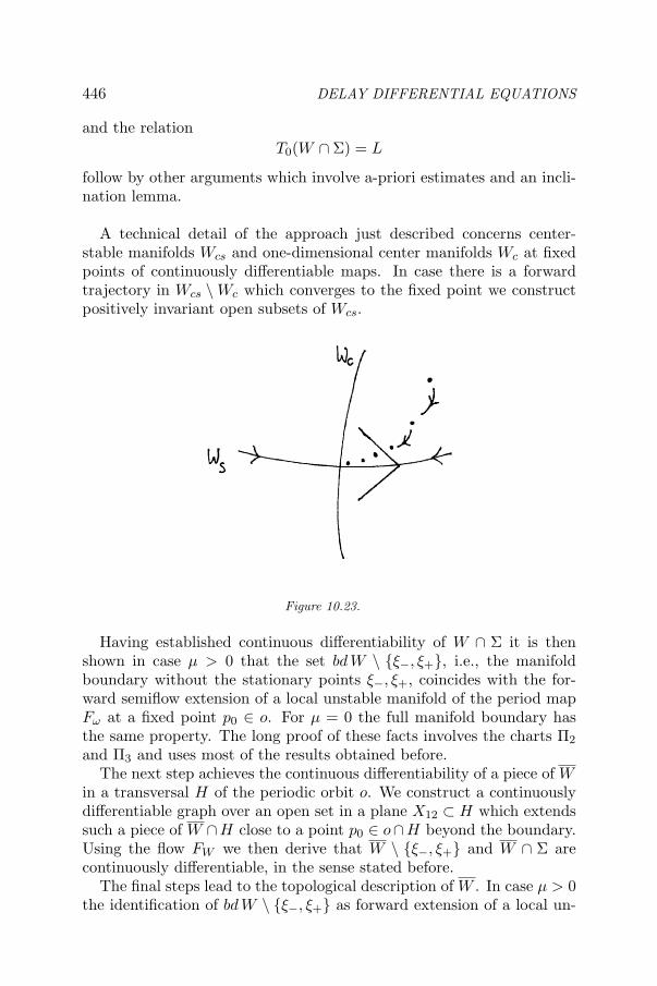
DELAY DIFFERENTIAL EQUATIONS
and the relationT0(W ∩ Σ) = L
follow by other arguments which involve a-priori estimates and an incli-nation lemma.
A technical detail of the approach just described concerns center-stable manifolds Wcs and one-dimensional center manifolds Wc at fixedpoints of continuously differentiable maps. In case there is a forwardtrajectory in Wcs \Wc which converges to the fixed point we constructpositively invariant open subsets of Wcs.
Figure 10.23.
Having established continuous differentiability of W ∩ Σ it is thenshown in case µ > 0 that the set bd W \ ξ−, ξ+, i.e., the manifoldboundary without the stationary points ξ−, ξ+, coincides with the for-ward semiflow extension of a local unstable manifold of the period mapFω at a fixed point p0 ∈ o. For µ = 0 the full manifold boundary hasthe same property. The long proof of these facts involves the charts Π2
and Π3 and uses most of the results obtained before.The next step achieves the continuous differentiability of a piece of W
in a transversal H of the periodic orbit o. We construct a continuouslydifferentiable graph over an open set in a plane X12 ⊂ H which extendssuch a piece of W ∩H close to a point p0 ∈ o∩H beyond the boundary.Using the flow FW we then derive that W \ ξ−, ξ+ and W ∩ Σ arecontinuously differentiable, in the sense stated before.
The final steps lead to the topological description of W . In case µ > 0the identification of bd W \ ξ−, ξ+ as forward extension of a local un-
446

Dynamics of Delay Differential Equations
Figure 10.24.
Figure 10.25.
447

DELAY DIFFERENTIAL EQUATIONS
stable manifold is used to define homeomorphisms from bd W onto theunit sphere S2 ⊂ R
3. Then a generalization due to Bing [29] of theSchoenfliess theorem [210] from planar topology is employed to obtainhomeomorphisms from W onto the closed unit ball in R
3. The applica-tion of Bing’s theorem requires to identify the bounded component ofthe complement of the set
Π3(bd W ) ∼= S2
in R3 as the set Π3W , and to verify that Π3W is uniformly locally 1-
connected. This means that for every ε > 0 there exists δ > 0 so thatevery closed curve in a subset of Π3W with diameter less than δ canbe continuously deformed to a point in a subset of Π3W with diameterless than ε. We point out that the proof of this topological propertyrelies on the smoothness of the set W \ ξ−, ξ+, and involves subsetsof boundaries of neighbourhoods of 0, ξ−, ξ+ in W which are transver-sal to the flow FW . In order to construct these smooth boundaries wehave to go back to the variation-of-constants formula for RFDEs in theframework of sun-dual and sun-star dual semigroups [57]. In case µ = 0the construction of the desired homeomorphism from W onto the solidcylinder is different but uses Bing’s theorem as well.
What can be said about W close to the attracting stationary pointsξ−, ξ+? Consider ξ+. The inclusion
W ⊂ ξ+ −K
implies that the tangent cone T0W is the singleton 0; therefore W andbd W are not smooth at ξ+.
Let C1+ denote the leading realified one-dimensional generalizedeigenspace associated with the variational equation along the solutionR t → ξ+ ∈ R. Analogously L+ is the realified 2-dimensional gener-alized eigenspace of the next pair of eigenvalues, and C3<+ is given bythe remaining eigenvalues. We have
C1+ = R · η+
with η+ ∈ C a segment of the associated positive decreasing exponentialsolution of the variational equation.
In [242] the singularity ξ+ is described in terms of the outward tangentcone T+bd W , defined as the set of tangent vectors c′(0) ∈ C of continu-ously differentiable curves c : (−ε, 0] → C, ε > 0, in bd W ending at ξ+,
448

Dynamics of Delay Differential Equations
and in terms of the set LTP of limit points of tangent planes Tφbd W ,φ = ξ+, as φ tends to ξ+. We prove
T+bd W = [0,∞) · η+
and show that LTP coincides with the set of planes in C1+ ⊕ L+ con-taining C1+.
Figure 10.26.
Convergence of finite-dimensional subspaces of C is here defined bythe gap topology, which is given by the Hausdorff distance of the com-pact intersections of two such spaces with the unit sphere. The proofsemploy a-priori estimates and inclination lemmas.
For narrower classes of nonlinearities g and for the parameters µ > 0and g′(0) > 0 in a certain smaller range than before, the periodic orbito is the only one of the semiflow, and the set W is in fact the globalattractor of F [136]. The first and basic ingredient of the proof is theuniqueness result. The equations covered include examples from neuralnetwork theory.
Let us state some open problems.
Recall the question whether W ∩Σ can be represented by a smoothmap from a subset of L into the complementary space C1 ⊕ C3<.
One may ask for diffeomorphisms instead of homeomorphisms fromDW onto the solid cylinder in case µ = 0, and from DW \χ−, χ+onto the unit ball without its north and south poles in case µ > 0.
The assumption g′(ξ−) < µ, g′(ξ+) < µ, which makes the semi-groups associated with the stationary points ξ−, ξ+ hyperbolic,might be relaxed.
449

DELAY DIFFERENTIAL EQUATIONS
How is the global attractor organized in case W is a proper subset?
We add a few remarks about the last question. Let us first consider sit-uations where A is a subset of the order interval φ ∈ C : ξ− ≤ φ ≤ ξ+.The segments of the solutions x : R → R with V (xt) = 2 for all t ∈ R
may form, together with the stationary point 0, a smooth disk-like sub-manifold A2 in A which extends W ∩ Σ beyond o and contains at leastone additional periodic orbit, forming the manifold boundary of A2.In this case, the unstable sets of the periodic orbits in A2 should beanalogues of bd W \ ξ−, ξ+, namely 2-dimensional invariant submani-folds given by heteroclinic connections from the periodic orbit to ξ− andξ+. These submanifolds should subdivide the 3-dimensional subset A≤2
of A formed by 0 and the segments of all solutions x : R → R withξ− ≤ x(t) ≤ ξ+ and V (xt) ≤ 2 for all t ∈ R into invariant layers; asection of A≤2 containing ξ− and ξ+ might have the structure shown bya sliced onion.
Figure 10.27.
It may be the case that A = A≤2. If A is strictly larger than A≤2 thenwe have to expect a finite number of analogues of the smooth disk A2,given by higher even values of V , and a more complicated variety ofheteroclinic connections, between periodic orbits in the same disk, be-tween periodic orbits in different disks, from periodic orbits and 0 to ξ−and ξ+, from 0 to periodic orbits and to ξ− and ξ+. Also connectionsfrom periodic orbits to 0 become possible. A Morse decomposition of Asimilar to the one constructed by Mallet-Paret [171] should be useful todescribe a part of these heteroclinic connections.
Suppose now that A is not confined to the order interval φ ∈ C : ξ− ≤φ ≤ ξ+, and there are zeros ξ∗ of g − µ id below ξ− and above ξ+ with
450

Dynamics of Delay Differential Equations
g′(ξ∗) > µ. One out of many possibilities is that the part of A in a certainneighbourhood of a stationary point ξ∗ ∈ C given by such a value ξ∗ looksjust as we began to sketch it for the case A ⊂ φ ∈ C : ξ− ≤ φ ≤ ξ+.
Figure 10.28.
3. Chaotic motionThis part describes steps of the proof in [153, 154], which yields existenceof chaotic solution behaviour for eq. (1.1) with µ = 0,
x(t) = g(x(t− 1)),
for functions g which satisfy the negative feedback condition. The resultin [154] was not the first one about existence of chaotic solutions of delaydifferential equations, but the first concerning slowly oscillating solutionsof equations with smooth nonlinearities. The nonlinearities consideredhave extrema. Recall that monotonicity implies that the attractor AS ofalmost all solutions is a disk, which excludes complicated behaviour ofslowly oscillating solutions.
Nevertheless the proof begins with odd functions g which satisfyg′(ξ) < 0 for all ξ ∈ R. For a function of this type there is a slowlyoscillating periodic solution y : R → R with the symmetry
y(t) = −y(t− 2)
and minimal period 4, whose orbit o ⊂ C is unstable and hyperbolic,with exactly one Floquet multiplier λ outside the unit circle [115]. Thismultiplier is real and simple. It follows that the period map F4 has one-dimensional local center and unstable manifolds at its fixed point y0 = η.We may assume y(−1) = 0 < y(−1). The linear hyperplane
H = φ ∈ C : φ(−1) = 0
451

DELAY DIFFERENTIAL EQUATIONS
is transversal to o at η. For an associated Poincare return map the fixedpoint η is hyperbolic with one-dimensional local unstable manifold Wu
and local stable manifold Ws of codimension 1 in H. Recall the abstractresult for maps in Banach spaces which guarantees chaotic trajectories ina neighbourhood of a homoclinic loop. The plan is to verify the hypothe-ses of this result for a modification of the map P , whose trajectories alltranslate into slowly oscillating solutions of a delay differential equationas before, with a nonlinearity g∗ of negative feedback type which coin-cides with g in a neighbourhood of the interval y(R). The first majorstep is to find such functions g∗ so that there is a solution z : R → R
which is homoclinic with respect to o, i.e.,with
zt → o as |t| → ∞, z0 /∈ o.
This is done as follows.
y is increasing on the initial interval, and
y(0) = ‖η‖ = max y.
Information about the eigenspace of the Floquet multiplier λ revealsthat Wu contains the segment z0 of a solution z : R → R of the originalequation with
z(0) > y(0)
so that for some ε > 0 and δ > 0,
z(t) > y(0) + ε on (−δ, 0], z(t) < y(0) + ε on (−∞,−δ).
The key to all is now a simple observation: Any modification g∗ of gin the interval (y(0) + ε,∞) preserves y and the restriction of z to theinterval
(−∞,−δ + 1]
as solutions, but affects the forward continuation of z|(−∞,−δ +1] as asolution z∗ : R → R of the new equation. Modifications g∗ are designedin such a way that the curves t → z∗t intersect the hyperplane H close toη at some t∗ > −δ +1. These modifications look rather complicated andhave several extrema: 3 local maxima and 4 local minima. Intersectionscan be achieved above and below the local stable manifold Ws, in acarefully chosen convex open neighbourhood N ⊂ H of η on which theoriginal map P is also a Poincare return map with respect to the modifieddelay differential equation, and
P (N ∩Ws) ⊂ N ∩Ws.
452

Dynamics of Delay Differential Equations
Figure 10.29.
Two such modifications g∗ are connected by a one-parameter-family.Continuity yields a member so that the intersection of the curve t → z∗twith H is on Ws, and the desired nonlinearity and homoclinic solutionare found.
Figure 10.30.
Now the map P is modified. The neighbourhood N has the prop-erty that it contains a backward trajectory (z∗tj )
0−∞ ∈ Wu of P so that
P (z∗t0) /∈ N ; z∗(t) = z(t) on (−∞, t0]. Choose a small closed ball B∗ ⊂ Ncentered at z∗t0 = zt0 = ζ, with z∗tj /∈ B∗ for j < 0 and so that one has anintersection map on B∗ which has the value t∗ − t0 at ζ. Redefine P onintB∗ using the previous intersection map, and keep P on N \ B∗ un-
453

DELAY DIFFERENTIAL EQUATIONS
changed. Then the fixed point η and the points z∗tj , j ≤ 0, z∗t∗ , P j(z∗t∗),j ∈ N, form a homoclinic loop of the new map P ∗.
Figure 10.31.
The previous construction is in fact carried out for families of one-parameter-families of nonlinearities. This freedom is needed for the re-maining part of the proof, which is to verify the transversality condition,namely, that there exists n0 ∈ N so that for all integers m < −n0 andn > n0, the points φm and φn of the homoclinic trajectory of P ∗ belongto Wu and Ws, respectively, with
D(P ∗)n−m(φm)TφmWu ⊕ TφmWs = H.
In our situation, codim Ws = 1. In order to verify the direct sumdecomposition of H we therefore need a suitable criterion for a vectorin H not to be tangent to the local stable manifold Ws. ’Suitable’means that the criterion should be sufficiently explicit in terms of thenonlinearity g∗ and the periodic solution y so that it can actually beapplied. The first step towards the transversality criterion concerns thevariational equation along y,
v(t) = g′(y(t− 1))v(t− 1)
and the monodromy operator M = DF4(η), η = y0. The monotonicityof g on the range of y implies that the set S of data with at mostone change of sign is again positively invariant, and that solutions v :[−1,∞)→ R starting in S are eventually slowly oscillating. The realifiedgeneralized eigenspace C≥ of the 2 leading Floquet multipliers on and
454

Dynamics of Delay Differential Equations
outside the unit circle is contained in S; dim C≥ = 2. Let Z denotethe complementary subspace given by the remaining spectrum of M ,i.e., the linear stable space of M . Recall that the local stable manifoldWs(η) of the period map F4 at η satisfies
TηWs(η) = Z.
Initial data in Z define solutions v : [−1,∞) → R with segments in C\S.So,
Z ∩ S = ∅,and if a solution v is eventually slowly oscillating then χ = v0 ∈ C \ Z;in other words, the initial value is transversal to Z. Here we have a firstsufficient condition for transversality, but not yet for the right map andonly at a particular point of the local stable manifold. In a next step itis shown that for any φ ∈Ws(η) and χ ∈ C,
χ ∈ C \ TφWs(η) if and only if vφ,χ is eventually slowly oscillating.
With regard to the proof, notice that for φ close to η the spaces TφWs(η)and Z are close. Flowlines starting in Ws(η) converge to o as t → ∞with asymptotic phase. This yields that the coefficient function in thevariational equation along xφ : [−1,∞) → R, which is satisfied by vφ,χ,approaches a shifted copy of the coefficient function in the variationalequation along the periodic solution y. - The main tool used in the proofis an inclination lemma in a non-hyperbolic situation.
The final form of the criterion, for the Poincare map P , is that forany φ ∈Ws and any χ ∈ H,
χ ∈ H \ TφWs
if and only if
for every pair of reals (a, b) = (0, 0), the function
(0,∞) t → a xφ(t) + b vφ,χ(t) ∈ R is eventually slowly oscillating.
Notice that for t > 1 the function considered here satisfies the variationalequation along the solution xφ : [−1,∞) → R. - The proof exploits therelation between derivatives of the Poincare map and the period map,and the asymptotic phase for flowlines starting in Ws.
The last part of the proof that chaotic motion exists is the search fora subclass of nonlinearities g∗ so that for all nonzero
χ ∈ D(P ∗)n(ζ)TζWu
455

DELAY DIFFERENTIAL EQUATIONS
and for all sufficiently large integers n the sufficient condition in the pre-vious ’transversality-by-oscillation’ criterion is fulfilled.
The nonlinearities for which the proof just described works look muchmore complicated than the unimodal functions in versions of eq. (1.1)with µ > 0 which are known from applications. A reason for this is thatg∗ was chosen in such a way that the curve t → z∗t through a point in Wu
close to η is driven far away from o and then returns to Ws within a shortinterval of length approximately 3. In a more recent paper Lani-Waydawas able to modify the method and obtain a result for nicer-looking uni-modal nonlinearities [150].
Let us mention some open problems.
It has not yet been proved that the Mackey-Glass and Lasota-Wazewska-Czyzewska equations generate chaotic flowlines. Theseare equations of the form (1.1) with µ > 0 and unimodal analyticnonlinearities.
The result presented here establishes chaotic dynamics only in asmall, thin set in state space, in a ’Cantor dust’, whereas numeri-cal experiments indicate that many if not almost all solutions arecomplicated for a variety of nonlinearities.
Other recent results on chaotic solutions of delay differential equationsare due to Lani-Wayda [151] and Lani-Wayda and Szrednicki [152].
4. Stable periodic orbitsIn many cases the dynamics of nonlinear autonomous delay differentialequations is structured by periodic orbits. Existence of periodic orbitshas been shown by several methods, notably by means of the ejectivefixed point principle, by Schauder’s theorem directly, by related indexand continuation arguments, and by more geometric arguments (planardynamics in the attractor of almost all solutions, Poincare-Bendixsontheorems). Much less could be achieved concerning stability and unique-ness of periodic orbits.
Consider eq. (1.1),
x(t) = −µx(t) + g(x(t− 1)),
for µ ≥ 0 and nonlinearities g : R → R of negative feedback type whichare continuous or better. As in part 1, the method of steps yields max-imal solutions x : [−1,∞) → R of the associated IVP and a continuous
456

Dynamics of Delay Differential Equations
semiflow F .
Recall that, in some contrast to the preceding remarks, there arespecial equations for which it is extremely easy to find slowly oscillatingperiodic solutions whose orbits in C seem very stable and attractive.The underlying observation for this is the following. If g is constanton some ray [β,∞), β > 0 and if initial data φj ∈ C, j = 1, 2, withφj(t) ≥ β coincide at t = 0 then the method of steps shows immediatelythat the corresponding solutions coincide on [0, 1], and consequently forall t ≥ 0. They depend only on the values g(β) and φ(0). It is then easyto design nonlinearities g as above so that all segments xt of solutionsx = xφ starting at φ ≥ β with φ(0) = β return after some time p > 0,i.e., xp ≥ β and x(p) = β. The segment xp is a fixed point of the solutionmap Fp and defines a periodic solution which has period p and is slowlyoscillating.
Figure 10.32.
Moreover, for every ψ ∈ C close to φ = xp the solution xψ has segmentswhich after some time merge into the periodic orbit
o = xt : t ∈ R.
457

DELAY DIFFERENTIAL EQUATIONS
This expresses extremely strong attraction towards the periodic orbit.Poincare return maps on transversals to o are locally constant, the deriv-ative at the fixed point on o is zero, its spectrum is the singleton 0and the periodic orbit is hyperbolic.
What has just been said is strictly limited to equations where the non-linearity g is constant on some interval. What happens if g is only closeto such a function but not constant on any nontrivial interval? The ap-proach sketched above fails. The general results on existence mentionedat the beginning may give existence, but nothing beyond. In the sequela rather elementary method from [243] is presented which in a sense fillsthe gap between the easily accessible, detailed results in special casesas before, and the little information for nonlinearities which are closeto these but not necessarily constant on any interval. The importantproperty is Lipschitz continuity, which in earlier work on eq. (1.1) hasnot been exploited. (In case of related equations with state-dependentdelay, however, Lipschitz continuity always played a role.).
Fix µ > 0, b > a > 0. For β > 0 and ε > 0 consider nonlinearities inthe set N(β, ε) of continuous odd functions g : R → [−b, b] which satisfy
−a− ε < g(ξ) < −a + ε for all ξ ≥ β.
For β and ε small, g ∈ N(β, ε) is steep on (0, β), and close to −a sign on[β,∞).
When convenient the associated semiflow will be denoted by Fg.
Initial data will be taken from the closed convex sets
A(β) = φ ∈ C : φ(t) ≥ β on [−1, 0], φ(0) = β.
On A(β) a return map can be found for β and ε sufficiently small.
Proposition. There exists w ∈ (0, 1) such that for β, ε small and forg ∈ N(β, ε), φ ∈ A(β) the solution xφ,g = xφ of eq. (1) is strictly below−β on [w,w + 1]. Furthermore, there exists q = qg(φ) > w + 1 so thatxφ,g increases on (w + 1, q) and reaches the level −β at t = q.
The proof relies on the fact that on [β,∞) and on (−∞, β] the func-tion g is close to −a sign and a sign, respectively. Using this and thevariation-of-constants formula one sees that on (0, 1] solutions startingin A(β) lie in a narrow tongue between 2 decreasing exponentials. Themethod of steps yields sharp estimates of the solutions also on the nextintervals of unit length. Moreover, derivatives can be estimated with
458

Dynamics of Delay Differential Equations
Figure 10.33.
Figure 10.34.
459

DELAY DIFFERENTIAL EQUATIONS
sufficient accuracy.
The return map R = Rg : A(β) → A(β) is then given by
R(φ) = −Fg(qg(φ), φ).
Notice that g being odd any fixed point φ of Rg defines a slowly oscil-lating periodic solution x : R → R of eq. (1) with the symmetry
x(t) = −x(t + qg(φ)) for all t ∈ R,
and minimal period p = 2q. Fixed points exist, due to Schauder’s the-orem. However, our objective is more than mere existence. Notice thatup to here only continuity of the nonlinearities in eq. (1) has been used.The next objective is to find an upper estimate of the Lipschitz constant
L(R) = supφ=ψ
‖R(φ)−R(ψ)‖‖φ− ψ‖ ≤ ∞
of R. This is facilitated by a decomposition of R = Rg into the restrictionof Fg,1 to A(β), followed by the restriction of Fg,w to Fg,1(A(β)), andfinally followed by the map
Fg,1+w(A(β)) ψ → −Fg(sg(ψ), ψ) ∈ A(β)
where s = sg(ψ) is defined by the equation
w + 1 + s = qg(φ) for all φ ∈ A(β) with ψ = Fg,1+w(φ).
(Observe that for all φ ∈ A(β) whose solutions coincide on [w,w+1] theargument qg(φ) is the same - it depends only on the behaviour of thesolutions on [w,w + 1].)
The Lipschitz constant L(Rg) will be estimated by an expressionwhich involves the Lipschitz constant L(g) of g and the Lipschitz con-stant
Lβ(g) = L(g|[β,∞)).
Notice that for each g ∈ N(β, ε), L(g) ≥ a−εβ is large for β > 0 small.
On the other hand, each N(β, ε) contains Lipschitz continuous functionsg so that Lβ(g) is arbitrarily small. This will be exploited later.
We derive Lipschitz estimates of the composites of the return map Rg
for g ∈ N(β, ε), with β and ε sufficiently small.
460

Dynamics of Delay Differential Equations
Proposition. L(Fg,1|A(β)) ≤ Lβ(g).
The proof is almost obvious from the facts that for φ, ψ in A(β) thevariation-of-constants formula says
Fg,1(φ)(t)− Fg,1(ψ)(t) = xφ,g(1 + t)− xψ,g(1 + t)
= 0− 0 +∫ 1+t
0e−µ(1+t−s)(g(φ(s− 1))− g(ψ(s− 1)))ds,
and that the arguments of g belong to [β,∞). In the same way one findsthe next result.
Proposition. L(Fg,w|Fg,1(A(β))) ≤ 1 + w L(g).
The difference to the previous proposition is due to the fact thatarguments of Fg,w may differ at t = 0, and traverse the interval [−β, β]where g is steep. One time unit later large deviations of one solutionfrom another become possible.
Next we need an estimate of the Lipschitz constant of the intersectionmap sg.
Proposition.
L(sg) ≤1 + eµ Lβ(g)a− ε− β µ eµ
The proof begins with the fact that for ψ = Fg,w+1(φ) with φ ∈ A(β)there is an equation defining qg(φ) and sg(ψ),
β = xφ,g(qg(φ)) = xφ,g(1 + w + sg(ψ)).
The last term is evaluated by the variation-of-constants formula on[1 + w, 1 + w + sg(ψ)]. The resulting equation for sg(ψ) and for somesg(ψ), ψ = Fg,1+w(φ), φ ∈ A(β), are subtracted from each other. Furtherelementary manipulations lead to the desired estimate.
Proposition.
L(Fg(sg(·), ·)|Fg,1+w(A(β))) ≤
L(sg) · [µ (1− a
µ(1− e−µ)) + maxb, a + ε] + 1 + Lβ(g).
The proof uses the triangle inequality, the preceding proposition, andarguments as in the proof of the estimate of L(Fg,w|Fg,1(A(β)).
461

DELAY DIFFERENTIAL EQUATIONS
Notice that L(Fg(sg(·), ·)| . . .) is bounded in terms of Lβ(g) and con-stants for β, ε small. So this term does not become large for suitableg ∈ N(β, ε).
The resulting estimate for the Lipschitz constant of the return map is
L(Rg) ≤ Lβ(g) (1 + w L(g))L(Fg(sg(·), ·)|Fg,1+w(A(β))).
A consequence is that there exist g ∈ N(β, ε) so that Rg is a contraction.Examples are found as follows. First fix β and ε so that the smallnesshypothesis for the previous estimate of L(Rg) holds for all g ∈ N(β, ε).Then choose a Lipschitz continuous odd function g : [−β, β] → [−b, b]which satisfies −a − ε < g(β) < −a + ε. Continue this function to anodd map on R with values in (−a − ε,−a + ε) on (β,∞) and Lβ(g) sosmall that the bound for L(Rg) is less than 1.
Remarks. The small constant Lβ(g) compensates diverging solutionbehaviour allowed by the factor 1+w L(g), on the way of flowlines backto −A(β). The nonlinearities g for which Rg is a contraction are notnecessarily constant on any interval, not necessarily monotone, may nothave limits at infinity, and may not be differentiable everywhere. Thenegative feedback condition may be violated in (−β, β). The orbits ofthe periodic solutions obtained from the fixed points of the contractingreturn maps attract all flowlines starting in A(β); one can show that incase g is continuously differentiable the periodic orbits are hyperbolicand stable.
A disadvantage of the previous Lipschitz estimate of L(Rg) is that itis not easy to verify for given analytic nonlinearities, which are steepclose to 0 and flat away from 0, and which arise in applications, like,e.g., the function
g = − tanh(γ·), γ > 0 large,
used in neural network theory. In [244] the approach described aboveis refined for nonlinearities g ∈ N(β, ε) which are monotone close to0. This involves sharp estimates of the divergent behaviour of flowlinesone time unit after the underlying solutions traverse the interval [−β, β]where g is monotone and steep. The improved Lipschitz estimates yieldcontracting return maps (and hyperbolic stable periodic orbits) for thescaled hyperbolic tangens above, for
g = − arctan(γ·), γ > 0 large,
and for other nonlinearities.
462

Dynamics of Delay Differential Equations
The sharpened estimates are obtained as follows. Let g ∈ N(β, ε) begiven. The tongue containing xφ,g, φ ∈ A(β), on [0, 1] is formed by thesolutions y> = y>,β,ε and y< = y<,β,ε of the IVPs
y = −µ y − a± ε, y(0) = β.
Define w = w(β, ε) to be the argument where y> reaches the level y =−β. For β not too large,
0 < w < 1.
Obviously,xφ,g(t) ≤ −β on [w, 1].
Let z< = z<,β,ε and z> = z>,β,ε denote the zeros of y< and y>, respec-tively, and let
β− = β−,β,ε = y<(w) < −β.
Figure 10.35.
For β and ε small and g ∈ N(β, ε) consider the return map Rg : A(β) →A(β) and decompose it as before. The objective is to find a better esti-mate for the middle composite Fg,w|Fg,1(A(β)). Recall that a Lipschitzcontinuous function g ∈ N(β, ε) is almost everywhere differentiable. Weneed the hypothesis that there is a set D ⊂ R whose complement hasLebesgue measure 0, with
g′(ξ) < 0 on D ∩ (β−, β),
g′ decreasing on D ∩ (β−, 0) and increasing on D ∩ (0, β).
Proposition.
L(Fg,w)|...) ≤ 4 + L(g)1µ
log(a + ε)(µβ + a− ε)(a− ε)(µβ + a + ε)
.
463

DELAY DIFFERENTIAL EQUATIONS
Figure 10.36.
Remark. The factors following L(g) replace the constant w in theformer estimate of L(Fg,w)|...). Notice that they vanish for ε = 0 ! Thisindicates that L(Fg,w|...) may not be too large even if L(g) is large, forβ and ε small.
The proof of the proposition begins with the extension of g′ to afunction on (β−, β) which is decreasing on (β−, 0) and increasing on(0, β). Let φ and ψ in Fg,1(A(β)) be given. For −1 ≤ t ≤ 0 and0 < w + t,
(Fg,w(φ)− Fg,w(ψ))(t) = xφ,gw (t)− xψ,g
w (t) =
(φ(0)− ψ(0))e−µ(w+t) +∫ w+t
0e−µ(w+t−s)(g(φ(s− 1))− g(ψ(s− 1)))ds,
|...| ≤ ‖φ− ψ‖+∫ w
0|g(φ(s− 1))− g(ψ(s− 1)))|ds.
In the last integral we have φ = x1 and ψ = z1 with solutions x :[−1,∞)→ R and z : [−1,∞)→ R which start in A(β),
∫ w
0|...|ds =
∫ w
0|g(x(s))− g(z(s))|ds.
In order to estimate the integrand, consider the interval Is with end-points x(s) and z(s), 0 ≤ s ≤ w. Obviously,
|g(x(s))− g(z(s))| = |∫
Is
g′|
≤ supIs
|g′| · |x(s)− z(s)| ≤ sup...
. . . ‖φ− ψ‖
464

Dynamics of Delay Differential Equations
and
β− ≤ y<(s) ≤ minx(s), z(s) ≤ maxx(s), z(s) ≤ y>(s) ≤ β,
orIs ⊂ [y<(s), y>(s)] ⊂ [β−, β].
The last relation shows that in case 0 < y<(s) (i.e., s < z<) themonotonicity property of g′ is applicable. We find
supIs
|g′| ≤ −g′(y<(s)).
In case 0 ∈ Is,supIs
|g′| = −g′(0).
In case y>(s) < 0 (i.e., z> < s),
supIs
|g′| ≤ −g′(y>(s)).
Figure 10.37.
Now the last integrals can be estimated as follows. We have∫ w
0|...| ≤ ‖φ− ψ‖ · (
∫ z<
0|g′ y<|+ |g′(0)|
∫ z>
z<
1 +∫ w
z>
|g′ y>|).
The substitution s = y−1< (ξ) in the first integral leads to the upper bound
1 for this integral. The substitution s = y−1> (ξ) in the third integral leads
to the upper bound 2 for it. The endpoints z< and z> of the range inthe second integral can be computed as functions of β, ε, µ, a.
In the remaining case w + t ≤ 0, clearly
|(Fg,w(φ)−Fg,w(ψ))(t)| = |xφ,gw (t)−xψ,g
w (t)| = |φ(w+t)−ψ(w+t)| ≤ ‖φ−ψ‖.
465

DELAY DIFFERENTIAL EQUATIONS
Remark. It can be shown that the Lipschitz estimate of the proposi-tion is optimal in the limit (β, ε) → (0, 0).
Continuing as in [243] one finds that for (β, ε) small and g ∈ N(β, ε),
L(Rg) ≤ Lβ(g) [4 + L(g)β ε3µ
a2]
·[ 1 + eµ Lβ(g)a− ε− µβ eµ
· [µ (1− a
µ(1− e−µ)) + maxb, a + ε] + 1 + Lβ(g)].
The middle factor comes from the estimate of the middle compositeFg,w|.... Recall that for suitable g ∈ N(β, ε), Lβ(g) is small.
How can one verify for given nonlinearities g that the upper boundfor L(Rg) is less than 1? Let µ > 0 and an odd bounded Lipschitzcontinuous function g : R → R be given so that g′ is negative andincreasing on the complement of a set of measure 0 in [0,∞). Then ghas a limit −a ≤ 0 at +∞. Suppose a > 0, and consider the family offunctions
gγ = g(γ·), γ > 0.
Figure 10.38.
How can β = β(γ) and ε = ε(γ) be chosen so that gγ ∈ N(β, ε) andL(Rgγ ) < 1, at least for large γ? We have Lβ(gγ) = γ Lγβ(g).
Proposition. Suppose there exists a function
β∗ : (0,∞) → (0,∞)
so that for γ →∞,
β∗(γ) → 0,
466

Dynamics of Delay Differential Equations
γ β∗(γ) →∞,
γ Lγβ∗(γ)(g) → 0,
γ Lγβ∗(γ)(g) γ β∗(γ) [a + g(γ β∗(γ))] → 0.
Then there exists γ∗ > 0 so that for all γ > γ∗, Rgγ is a contraction.
In order to prove this one sets b = 2a. For every γ > 0, β > 0, andε = a + g(γ β), we have
gγ ∈ N(β, ε).
The function gγ is Lipschitz continuous and satisfies the monotonicityhypothesis required for the last proposition. Then the estimate of L(Rgγ )has to be used.
Examples. Consider µ > 0 and g as before. Suppose in addition thatfor some r > 3
2 ,
D ∩ (0,∞) ξ → |ξrg′(ξ)| is bounded.
Choose s ∈ (−1, 0) with 11+s < r and 1 + 1
2+2s < r. Then the map
β∗ : γ → γs
satisfies the hypotheses of the last proposition.
Special cases are given by g = − tanh, g = − arctan.
Remarks. A somewhat stronger result for one-parameter-families ofnonlinearities gγ which are at least continuously differentiable was ob-tained earlier by Xie [255]. He proved that for γ large the orbits of givenperiodic solutions are hyperbolic and stable. The proof is a study ofthe leading Floquet multipliers and relies on very careful a-priori esti-mates of periodic solutions. The hypotheses needed in [255] are that thesmooth function g has limits at infinity, that g′ is Lebesgue integrable,and that ξ g′(ξ) → 0 as |ξ| → ∞. I.e., no monotonicity properties of g′
are required, and the behaviour of g′ at infinity is less restricted than inthe examples mentioned above.
In the approach described here the condition that the nonlinearities gare odd is not essential. Variants of the method have also been appliedto systems of delay differential equations [246, 96] and to an equationwith state-dependent delay [245]. For the latter, no other method toobtain stable periodic motion seems presently available.
467

DELAY DIFFERENTIAL EQUATIONS
5. State-dependent delays
Differential equations with state-dependent delay can often be writtenin the form
x(t) = f(xt) (5.1)
with a continuously differentiable map f : C1 ⊃ U → Rn, U open. The
associated IVP is not well-posed on U , however. Continuous flowlinesmay in general only be expected for data in the subset
X = Xf = φ ∈ U : φ(0) = f(φ) ⊂ C1.
Notice that X is a nonlinear version of the positively invariant domain
φ ∈ C1 : φ(0) = Lφ
of the generator G of the semigroup defined by the linear autonomousRFDE
y(t) = Lyt
on the larger space C, for L : C → Rn linear continuous. Notice also
that in case of a locally Lipschitz continuous map f∗ : U∗ → Rn, U∗ ⊂ C
open, all solutions x : [−h, b) → Rn, h < b, of the RFDE
x(t) = f∗(xt)
satisfy
xt ∈ Xf∗ = φ ∈ U∗ ∩ C1 : φ(0) = f∗(φ) for h ≤ t < b.
I.e., the set Xf∗ absorbs all flowlines on intervals [−h, b) which are longenough. In particular, Xf∗ contains all segments of solutions on intervals(−∞, b), b ≤ ∞ - equilibria, periodic orbits, local unstable manifolds,and the global attractor if the latter is present.
In order to have a semiflow on X with differentiability properties weneed that X is smooth. This requires an additional condition on f .
Proposition. Suppose X = ∅ and(P1) each derivative Df(φ), φ ∈ U, has a continuous linear extension
Def(φ) : C → Rn.
Then X is a continuously differentiable submanifold of C1 with codi-mension n.
468

Dynamics of Delay Differential Equations
The proof is easy. Consider the continuous linear map
p : C1 φ → φ(0) ∈ Rn.
ThenX = (p− f)−1(0).
It is enough to show that all derivatives D(p− f)(φ), φ ∈ X, are surjec-tive.Proof of this for n = 1: By (P1), for some δ > 0,
Def(φ)Cδ ⊂ (−1, 1).
There exists χ ∈ C1 ∩ Cδ with χ(0) = 1. Hence
0 < χ(0)−Df(φ)χ = D(p− f)(φ)χ,
R ⊂ D(p− f)(φ)C1.
(The Implicit Function Theorem then yields that close to φ the set X isgiven by a map from a subset of the nullspace N of D(p− f)(φ) into acomplement of N in C1.)
A solution of eq. (5.1) is defined to be a continuously differentiablemap x : [t0 − h, te) → R
n, with t0 ∈ R and t0 < te ≤ ∞, so that fort0 ≤ t < te, xt ∈ U , and eq. (5.1) is satisfied. We also consider solutionson unbounded intervals (−∞, te). Maximal solutions of IVPs are definedas in part I.
Theorem. Suppose (P1) holds, X = ∅, and(P2) for each φ ∈ U there exist a neighbourhood V (in C1) and L ≥ 0so that
|f(ψ)− f(χ)| ≤ L‖ψ − χ‖ for all ψ ∈ V, χ ∈ V.
Then the maximal solutions xφ : [−h, te(φ)) → Rn of eq. (5.1) which
start at points φ ∈ X define a continuous semiflow
F : Ω (t, φ) → xφt ∈ X, Ω =
⋃φ∈X
[0, te(φ))× φ,
and all solution maps
Ft : Ωt φ → F (t, φ) ∈ X, ∅ = Ωt = φ ∈ X : (t, φ) ∈ Ω,
are continuously differentiable. For all φ ∈ X, t ∈ [0, te(φ)), and χ ∈TφX,
DFt(φ)χ = vφ,χt
469

DELAY DIFFERENTIAL EQUATIONS
with a continuously differentiable solution vφ,χ : [−h, te(φ)) → Rn of the
IVPv(t) = Df(Ft(φ))vt,
v0 = χ.
Comments.
Notice that the Lipschitz estimate in (P2) involves the smallernorm ‖ · ‖ ≤ ‖ · ‖1 on the larger space C ⊃ C1. Property (P2)was used in [245] in a proof that for certain differential equationswith state-dependent delay stable periodic orbits exist. It is closelyrelated to the earlier idea of being locally almost Lipschitzian inwork of Mallet-Paret, Nussbaum, and Paraskevopoulos [175].
Property (P1) is a special case of a condition used in Krisztin’swork on smooth unstable manifolds [132]. Almost the same prop-erty occurred earlier [175], under the name almost Frechet differ-entiability.
Louihi, Hbid, and Arino [164] identified the set X as the domainof a generator in the context of nonlinear semigroup theory, fora class of differential equations with state-dependent delay. It ismentioned in [164] that X is a Lipschitz manifold. In [139] acomplete metric space analogous to X serves as a state space forneutral functional differential equations.
Former results about solutions close to an equilibrium, like theprinciple of linearized stability for differential equations with state-dependent delay due to Cooke and Huang [48], or results on localunstable manifolds [131, 132], had to be proven without knowledgeof linearizations at the equilibrium. The difficulty was circum-vented by means of an associated linear autonomous RFDE (a) onthe large space C. Eq. (a) is obtained heuristically, for certainclasses of differential equations with state-dependent delay: Firstthe delays are frozen at the given equilibrium φ, then the resultingRFDE with constant delays is linearized. Examples show how eq.(a) is related to the actual variational equation
v(t) = Df(φ)vt
for data in TφX ⊂ C1: Eq. (a) is simply
v(t) = Def(φ)vt.
470

Dynamics of Delay Differential Equations
Also, for the semigroup (T (t))t≥0 on C associated with the lastRFDE and for its generator G,
TφX = dom(G)
andDFt(φ)χ = T (t)χ on TφX.
The theorem yields continuously differentiable local invariant man-ifolds
Wu, Wc, Ws
of the solution maps Ft at fixed points; in particular, at stationarypoints φ of the semiflow. In the last case the tangent spaces ofthe local invariant manifolds at φ are the unstable, center, andrestricted stable spaces
Cu, Cc, and Cs ∩ TφX
of the generator G, respectively. At a stationary point φ the localunstable and stable manifolds Wu, Ws coincide with local unstableand stable manifolds W u, W s of the semiflow F . An analogousresult for - suitable - center manifolds seems unknown.
Local unstable manifolds at stationary points of differential equa-tions with state-dependent delay were found earlier by H. Krishnan[131] and T. Krisztin [132], under the hypothesis that the associ-ated linear autonomous RFDE (a) is hyperbolic. Hyperbolicity isalso necessary for a recent result of Arino and Sanchez [16] whichcaptures saddle point behaviour of solutions close to equilibriumfor a class of differential equations with state-dependent delay.
The essential part of the proof of our theorem is to solve the equation
x(t) = φ(0) +∫ t
0f(xs)ds, 0 ≤ t ≤ T,
x0 = φ ∈ X,
by a continuously differentiable map
x : [−h, T ] → Rn,
for φ ∈ X given; x should also be continuously differentiable with respectto φ. Is the Contraction Mapping Principle with parameters applicable?How does the operator given by the fixed point equation depend on φ?We first rewrite the fixed point equation so that the dependence of the
471

DELAY DIFFERENTIAL EQUATIONS
integral on φ becomes explicit. For φ ∈ C1 let φ denote the continuouslydifferentiable extension to [−h, T ] given by
φ(t) = φ(0) + φ(0)t on [0, T ].
Set u = x− φ. Then u belongs to the Banach space C10T of continuously
differentiable maps y : [−h, T ]→ Rn with
y(t) = 0 on [−h, 0];
the norm on C10T is given by
‖y‖C10T
= max−h≤t≤T
|y(t)|+ max−h≤t≤T
|y(t)|.
u and φ satisfy
u(t) + φ(t) = φ(0) +∫ t
0f(us + φs)ds
andφ(t) = φ(0) + φ(0)t = φ(0) + t f(φ)
(since φ ∈ X)
= φ(0) +∫ t
0f(φ)ds.
For u ∈ C10T this yields the fixed point equation
u(t) =∫ t
0(f(us + φs)− f(φ))ds, 0 ≤ t ≤ T,
with parameter φ ∈ X.
Now let some φ0 ∈ X be given. For φ ∈ X close to φ0, u ∈ C10T small,
and 0 ≤ t ≤ T with T > 0 small, define
A(φ, u)(t)
by the right hand side of the last equation. The property (P2) is used toshow that the maps A(φ, ·) are contractions with respect to the norm onC1
0T , with a contraction factor independent of φ: Let v = A(φ, u), v =A(φ, u). For 0 ≤ t ≤ T ,
|v(t)− v(t)| = |f(ut + φt)− f(ut + φt)| ≤ L‖ut − ut‖
(due to (P2); L may be large!)
≤ L max0≤s≤T
|u(s)− u(s)|.
472

Dynamics of Delay Differential Equations
We exploit the fact that the last term does not contain derivatives: For0 ≤ s ≤ T ,
|u(s)− u(s)| = |0− 0 +∫ s
0(u(r)− u(r))dr| ≤ T‖u− u‖C1
0T.
Hence|v(t)− v(t)| ≤ L T ‖u− u‖C1
0T.
Also,
|v(t)− v(t)| = |∫ t
0(f(us + φs)− f(us + φs))ds| ≤ L T max
0≤s≤t‖us − us‖
≤ L T ‖u− u‖C10T
.
(Property (P2) is not necessary here. Alternatively the local Lipschitzcontinuity of f with respect to the norm on C1 can be used to find asuitable upper estimate.)
For 2 L T < 1 the map A(φ, ·) becomes a contraction. One finds aclosed ball which is mapped into itself by each map A(φ, ·). The formuladefining A shows that A is continuously differentiable. It follows that foreach φ the ball contains a fixed point uφ of A(φ, ·) which is continuouslydifferentiable with respect to φ. This completes the essential step in theproof of the theorem.
We give an example which is based on elementary physics. Consideran object on a line which attempts to regulate its position x(t) by echo.The object emits a signal which is then reflected by an obstacle. The re-flected signal is detected and the signal running time is measured. Fromthis a position is computed (which is not necessarily the true position).The computed position is followed by an acceleration towards a pre-ferred position (e.g., an equilibrium position in a certain distance fromthe obstacle).
Let c > 0 denote the speed of the signals, −w < 0 the position of theobstacle, and µ > 0 a friction constant. The acceleration is given by afunction a : R → R; one may think of negative feedback:
a(0) = 0 and ξ a(ξ) < 0 for ξ = 0.
Let x(t) denote the position of the object at time t, v(t) its velocity, p(t)the computed position, and s(t) the running time of the signal which has
473

DELAY DIFFERENTIAL EQUATIONS
been emitted at time t− s(t) and whose reflection is detected at time t.The model equations then are
x(t) = v(t)
v(t) = −µv(t) + a(p(t))
p(t) =c
2s(t)− w
c s(t) = x(t− s(t)) + x(t) + 2w
Here only solutions with−w < x(t)
are considered. The formula defining p(t) yields the true position if
x(t) = x(t− s(t)),
which holds at least at equilibria.
Let w+ > 0. Restrict attention further to bounded solutions with
−w < x(t) < w+ and |x(t)| < c.
Then necessarily
0 < s(t) ≤ 2w + 2w+
c= h.
The model has not yet the form (3) considered in the theorem. Inorder to reformulate the model, take h as just defined, consider thespace
C1 = C1([−h, 0], R2),
and the open convex subset
U = φ = (φ1, φ2) ∈ C1 : −w < φ1(t) < w+, |φ1(t)| < c for −h ≤ t ≤ 0.
Each φ ∈ U determines a unique solution s = σ(φ) of
s =1c(φ1(−s) + φ1(0) + 2w),
as the right hand side of this fixed point equation defines a contractionon [0, h]. The Implicit Function Theorem shows that the resulting map
σ : U → [0, h]
is continuously differentiable. Elementary estimates imply that it is alsoLipschitz continuous with respect to the norm on C = C([−h, 0], R2).
474

Dynamics of Delay Differential Equations
I.e., an analogue of property (P2) holds.
Assume the response function a : R → R is continuously differentiable.Then the map
f : U → R2
given byf1(φ) = φ2(0),
and
f2(φ) = −µφ2(0) + a(c
2σ(φ)− w) = −µφ2(0) + a
(φ1(−σ(φ)) + φ1(0)
2
)
is continuously differentiable and has property (P2), and for boundedsolutions as above the model can be rewritten in the form of eq. (5.1).
Verification of property (P1). For each φ ∈ U and all χ ∈ C1,
Dσ(φ)χ =Ev1(χ1,−σ(φ)) + Ev1(χ1, 0)
Ev1(φ1,−σ(φ))− c=
χ1(−σ(φ)) + χ1(0)φ1(−σ(φ))− c
,
with the evaluation map
Ev1 : C1([−h, 0], R)× [−h, 0] (ψ, t) → ψ(t) ∈ R.
Each Ev1(·, t), t ∈ [−h, 0], is the restriction of a continuous linear evalua-tion functional on the space C([−h, 0], R). It follows that Dσ(φ) : C1 →R has a continuous linear extension Deσ(φ) : C → R. The formula
Df2(φ)χ = −µEv1(χ2, 0) + Da(c
2σ(φ)− w)
c
2Dσ(φ)χ
finally shows that f has property (P1).
Supposea(0) = 0.
Then φ = 0 is a stationary point, and
σ(0) =2w
c.
The previous calculations show that the variational equation from thetheorem is the system
v1(t) = v2(t)
v2(t) = −µv2(t) + a′(0)v1(t− 2w/c) + v1(t)
2.
475
DELAY DIFFERENTIAL EQUATIONS
Notice that the heuristic approach (freeze the delay, then linearize) yieldsthe very same system.
Back to general results. The semiflow F from the theorem is continu-ously differentiable for t > h provided f satisfies (P1) and the conditionthat(P1∗) the map U × C (φ, χ) → Def(φ)χ ∈ R
n is continuous.
Remarks.
Notice that continuous differentiability of the semiflow (for t > h)is needed in order to have Poincare return maps for periodic orbits,among others.
(P1) and (P1∗) imply (P2).
(P1∗) holds for the example.
The stronger condition that the map
U φ → Def(φ) ∈ L(C, Rn)
be continuous is not satisfied by the example.
The solution maps Ft are compact for t ≥ h under certain otherhypotheses on f . The latter are satisfied by the example for suitablefunctions a.
Further work, Open Problems.
For continuously differentiable center manifolds of the semiflow,see the forthcoming survey article [107] and [134]. A first Hopfbifurcation theorem for differential equations with state-dependentdelay is due to M. Eichmann [62].
Can the approach be generalized so that one obtains higher orderderivatives for semiflows given by differential equations with state-dependent delay?
For suitable parameters stable periodic motion far away from equi-librium was established in [248].
A related but in several respects more complicated problem is thedescription of the motion of two charged particles, which was ini-tiated by R.D. Driver [61].
476

Chapter 11
DELAY DIFFERENTIAL EQUATIONS INSINGLE SPECIES DYNAMICS
S. Ruan∗
Department of MathematicsUniversity of MiamiPO Box 249085Coral Gables, FL [email protected]
1. IntroductionTime delays of one type or another have been incorporated into biolog-
ical models to represent resource regeneration times, maturation periods,feeding times, reaction times, etc. by many researchers. We refer to themonographs of Cushing (1977a), Gopalsamy (1992), Kuang (1993) andMacDonald (1978) for discussions of general delayed biological systems.In general, delay differential equations exhibit much more complicateddynamics than ordinary differential equations since a time delay couldcause a stable equilibrium to become unstable and cause the populationsto fluctuate. In this survey, we shall review various delay differentialequations models arising from studying single species dynamics.
Let x(t) denote the population size at time t; let b and d denote thebirth rate and death rate, respectively, on the time interval [t, t + ∆t],where ∆t > 0. Then
x(t + ∆t) − x(t) = bx(t)∆t − dx(t)∆t.
Dividing by ∆t and letting ∆t approach zero, we obtain
∗Research was partially supported by NSF grant DMS-0412047 and a Small Grant Awardfrom the University of Miami.
© 2006 Springer.
477
O. Arino et al. (eds.), Delay Differential Equations and Applications, 477–517.

478 DELAY DIFFERENTIAL EQUATIONS
dx
dt= bx − dx = rx, (1.1)
where r = b − d is the intrinsic growth rate of the population. Thesolution of equation (1.1) with an initial population x(0) = x0 is givenby
x(t) = x0ert. (1.2)
The function (1.2) represents the traditional exponential growth if r > 0or decay if r < 0 of a population. Such a population growth, due toMalthus (1798), may be valid for a short period, but it cannot go onforever. Taking the fact that resources are limited into account, Verhulst(1836) proposed the logistic equation
dx
dt= rx
(1 − x
K
), (1.3)
where r(> 0) is the intrinsic growth rate and K(> 0) is the carrying ca-pacity of the population. In model (1.3), when x is small the populationgrows as in the Malthusian model (1.1); when x is large the members ofthe species compete with each other for the limited resources. Solving(1.3) by separating the variables, we obtain (x(0) = x0)
x(t) =x0K
x0 − (x0 − K)e−rt. (1.4)
If x0 < K, the population grows, approaching K asymptotically ast → ∞. If x0 > K, the population decreases, again approaching Kasymptotically as t → ∞. If x0 = K, the population remains in time atx = K. In fact, x = K is called an equilibrium of equation (1.3). Thus,the positive equilibrium x = K of the logistic equation (1.3) is globallystable; that is, lim
t→∞x(t) = K for solution x(t) of (1.3) with any initial
value x(0) = x0.
2. Hutchinson’s EquationIn the above logistic model it is assumed that the growth rate of a
population at any time t depends on the relative number of individualsat that time. In practice, the process of reproduction is not instanta-neous. For example, in Daphnia a large clutch presumably is determinednot by the concentration of unconsumed food available when the eggshatch, but by the amount of food available when the eggs were forming,some time before they pass into the broad pouch. Between this timeof determination and the time of hatching many newly hatched animalsmay have been liberated from the brood pouches of other Daphnia in

DDE in Single Species Dynamics 479
the culture, so increasing the population. In fact, in an extreme case allthe vacant spaces K −x might have been filled well before reproductionstops. Hutchinson (1948) assumed egg formation to occur τ units oftime before hatching and proposed the following more realistic logisticequation
dx
dt= rx(t)
[1 − x(t − τ)
K
], (2.1)
where r and K have the same meaning as in the logistic equation (1.3),τ > 0 is a constant. Equation (2.1) is often referred to as the Hutchin-son’s equation or delayed logistic equation.
2.1 Stability and BifurcationThe initial value of equation (2.1) is given by
x(θ) = φ(θ) > 0, θ ∈ [−τ, 0],
where φ is continuous on [−τ, 0]. An equilibrium x = x∗ of (2.1) is stableif for any given ε > 0 there is a δ > 0 such that |φ(t)−x∗| ≤ δ on [−τ, 0]implies that all solutions x(t) of (2.1) with initial value φ on [−τ, 0]satisfy |x(t) − x∗| < ε for all t ≥ 0. If in addition there is a δ0 > 0 suchthat |φ(t) − x∗| ≤ δ0 on [−τ, 0] implies lim
t→∞x(t) = x∗, then x∗ is called
asymptotically stable.Notice that equation (2.1) has equilibria x = 0 and x = K. Small
perturbations from x = 0 satisfy the linear equation dxdt = rx, which
shows that x = 0 is unstable with exponential growth. We thus onlyneed to consider the stability of the positive equilibrium x = K. LetX = x − K. Then,
dX
dt= −rX(t − τ) − r
KX(t)X(t − τ).
Thus, the linearized equation is
dX
dt= −rX(t − τ). (2.2)
We look for solutions of the form X(t) = ceλt, where c is a constant andthe eigenvalues λ are solutions of the characteristic equation
λ + re−λτ = 0, (2.3)
which is a transcendental equation. By the linearization theory, x = K isasymptotically stable if all eigenvalues of (2.3) have negative real parts.

480 DELAY DIFFERENTIAL EQUATIONS
Set λ = µ + iν. Separating the real and imaginary parts of the char-acteristic equation (2.3), we obtain
µ + re−µτ cos ντ = 0,ν − re−µτ sin ντ = 0.
(2.4)
Notice that when τ = 0, the characteristic equation (2.3) becomes λ+r =0 and the eigenvalue λ = −r < 0 is a negative real number. We seekconditions on τ such that Reλ changes from negative to positive. By thecontinuity, if λ changes from −r to a value such that Reλ = µ > 0 whenτ increases, there must be some value of τ, say τ0, at which Reλ(τ0) =µ(τ0) = 0. In other words, the characteristic equation (2.3) must havea pair of purely imaginary roots ±iν0, ν0 = ν(τ0). Suppose such is thecase. Then we have
cos ν0τ = 0,
which implies that
νoτk =π
2+ 2kπ, k = 0, 1, 2, . . . .
Noting that νo = r, we have
τk =π
2r+
2kπ
r, k = 0, 1, 2, . . .
Therefore, whenτ = τ0 =
π
2r,
equation (2.3) has a pair of purely imaginary roots ±ir, which are simpleand all other roots have negative real parts. When 0 < τ < π
2r , all rootsof (2.3) have strictly negative real parts.
Denote λ(τ) = µ(τ) + iν(τ) the root of equation (2.3) satisfyingµ(τk) = 0, ν(τk) = ν0, k = 0, 1, 2, . . . We have the transversality con-dition
dµ
dτ
∣∣∣∣τ=τk
= r2 > 0, k = 0, 1, 2, . . .
We have just shown the following conclusions.
Theorem 1 (i) If 0 ≤ rτ < π2 , then the positive equilibrium x = K
of equation ( 2.1) is asymptotically stable.
(ii) If rτ > π2 , then x = K is unstable.
(iii) When rτ = π2 , a Hopf bifurcation occurs at x = K; that is, periodic
solutions bifurcate from x = K. The periodic solutions exist forrτ > π
2 and are stable.

DDE in Single Species Dynamics 481
K
/2r0
x
τπ
Figure 11.1. The bifurcation diagram for equation (2.1).
K
x
0t t 11 t 1+τ t 1+2τ t 111
+3τ t 1+4τ
Figure 11.2. The periodic solution of the Hutchinson’s equation (2.1).
The above theorem can be illustrated by Fig. 11.1, where the solidcurves represent stability while the dashed lines indicate instability.
By (iii), the Hutchinson’s equation (2.1) can have periodic solutionsfor a large range of values of rτ , the product of the birth rate r andthe delay τ . If T is the period then x(t + T ) = x(t) for all t. Roughlyspeaking, the stability of a periodic solution means that if a perturbationis imposed the solution returns to the original periodic solution as t → ∞with possibly a phase shift. The period of the solution at the criticaldelay value is 2π
ν0(Hassard et al. (1981)), thus, it is 4τ (see Fig. 11.2).
Numerical simulations are given in Fig. 11.3.
2.2 Wright ConjectureThe Hutchinson’s equation (2.1) can be written as
dy
dt= −ry(t − τ)[1 + y(t)]

482 DELAY DIFFERENTIAL EQUATIONS
0.4
0.6
0.8
1
1.2
1.4
1.6
1.8
x(t)
0 50 100 150 200 250 300t - time
tau=8
tau=11
Figure 11.3. Numerical simulations for the Hutchinson’s equation (2.1). Here r =0.15, K = 1.00. (i) When τ = 8, the steady state x∗ = 1 is stable; (ii) When τ = 11,a periodic solution bifurcated from x∗ = 1.
by assuming y(t) = −1 + x(t)/K. Letting t = τt, y(t) = y(τ t), we have
d
dty(t) = −rτy(t − 1)[1 + y(t)].
Denoting α = rτ and dropping the bars, we obtain
dy
dt= −αy(t − 1)[1 + y(t)]. (2.5)
By Theorem 1, we know that the zero solution of (2.5) is asymptoticallystable if α < π/2 and unstable if α > π/2. Wright (1955) showed thatthe zero solution of (2.5) is globally stable if α < 3/2. Wright thenconjectured that the zero solution of (2.5) is globally stable if α < π/2,which is still open.
Kakutani and Markus (1958) proved that all solutions of (2.5) oscil-late if α > 1/e and do not oscillate if α < 1/e. Jones (1962a, 1962b)studied the global existence of periodic solutions for α > π/2. For fur-ther research on existence of non-constant periodic solutions, see Hadelerand Tomiuk (1977), Hale and Verduyn Lunel (1993), Kaplan and York(1975), Naussbaum (1974), Walther (1975), etc. See also Kuang (1993)for further results and more references.
Recently, some attention has been paid to the study of equation (2.5)when α = α(t) is a positive continuous function. For example, Sugie(1992) showed that the zero solution of (2.5) with α = α(t) is uniformlystable if there is a constant α0 > 0 such that
α(t) ≤ α0 <32
for all t ≥ 0. (2.6)

DDE in Single Species Dynamics 483
Chen et al. (1995) improved condition (2.6) to the following:∫ t
t−1α(s)ds ≤ α0 <
32
for t ≥ 1. (2.7)
Stability conditions such as (2.6) and (2.7) are called 32−stability criteria.
For further related work, we refer to Kuang (1993), Yu (1996) and thereferences therein.
2.3 Instantaneous DominanceConsider a logistic equation with a discrete delay of the form
dx
dt= rx(t)[1 − a1x(t) − a2x(t − τ)], (2.8)
where a1 and a2 are positive constants. There is a positive equilibriumx∗ = 1
a1+a2, which is stable when there is no delay. Employing similar
arguments, one can prove the following results.
Theorem 2 (i) If a1 ≥ a2, then the steady state x∗ = 1a1+a2
is as-ymptotically stable for all delay τ ≥ 0.
(ii) If a1 < a2, then there is a critical value τ0 given by
τ0 =a1 + a2
r√
a22 − a2
1
arcsin
√a2
2 − a21
a2,
such that x∗ = 1a1+a2
is asymptotically stable when τ ∈ [0, τ0) andunstable when τ > τ0. A Hopf bifurcation occurs at x∗ when τpasses through τ0.
The above result indicates that if a1 ≥ a2, that is, if the instantaneousterm is dominant, then the steady state x∗ = 1
a1+a2is asymptotically
stable for all delay τ ≥ 0. In fact, we can show that it is asymptoticallystable for any initial value, that is, globally stable.
Theorem 3 If a1 > a2, then the steady state x∗ = 1a1+a2
of ( 2.8) isglobally stable.
Proof. Suppose x is a continuous function from [−τ, r) to R anddenote xt(θ) = x(t + θ), θ ∈ [−τ, 0]. Choose a Lyapunov function of theform
V (x(t), xt(θ)) = x − x∗ − x∗ lnx
x∗ + ξ
∫ 0
−τ[xt(θ)]2dθ, (2.9)

484 DELAY DIFFERENTIAL EQUATIONS
where ξ > 0 is a constant to be determined. Rewrite equation (2.8) asfollows:
dx
dt= rx(t)[−a1(x(t) − x∗) − a2(x(t − τ) − x∗)]. (2.10)
Then we havedV
dt
∣∣∣∣(2.10)
=dx
dt
x − x∗
x+ ξ[(x(t) − x∗)2 − (x(t − τ) − x∗)2]
= −(ra1 − ξ)[x(t) − x∗]2 + ra2[x(t) − x∗][x(t − τ) − x∗]+ξ[x(t − τ) − x∗]2.
If a1 > a2, choose ξ = 12ra1, so dV
dt |(2.10) is negatively definite and theresult follows.
3. Recruitment Models
3.1 Nicholson’s Blowflies ModelThe Hutchinson’s equation (2.1) can be used to explain several ex-
perimental situations, including Nicholson’s (1954) careful experimentaldata of the Australian sheep-blowfly (Lucila cuprina). Over a period ofnearly two years Nicholson recorded the population of flies and observeda regular basic periodic oscillation of about 35-40 days. To apply theHutchinson’s equation (2.1), K is set by the food level available, τ isapproximately the time for a larva to mature into an adult. The onlyunknown parameter is r, the intrinsic growth rate of the population. Ifwe take the observed period as 40 days, then the delay is about 9 days:the actual delay is about 15 days.
To overcome the discrepancy in estimating the delay value, Gurneyet al. (1980) tried to modify Hutchinson’s equation. Notice that Nichol-son’s data on blowflies consist primarily of observations of the time vari-ation of adult population. Let x(t) denote the population of sexuallymature adults. Then the rate of change of x(t) is the instantaneous rateof recruitment to the adult population R(t) minus the instantaneoustotal death rate D(t) :
dx
dt= R(t) − D(t).
To express R(t) we have to consider the populations of all the variousstages in the life-history of the species concerned and make the followingassumptions:
(i) all eggs take exactly τ time units to develop into sexually matureadults;

DDE in Single Species Dynamics 485
(ii) the rate at which the adult population produces eggs depends onlyon its current size;
(iii) the probability of a given egg maturing into a viable adult dependsonly on the number of competitors of the same age.
These imply that the rate of recruitment at time t + τ is a functiononly of the instantaneous size of the adult population at time t. Assumethat the average per capita fecundity drops exponentially with increasingpopulation, thus
R(t + τ) = θ(x(t)) = Px(t) exp[−x(t)/x0],
where P is the maximum per capita daily egg production rate, x0 is thesize at which the blowflies population reproduces at its maximum rate,and δ is the per capita daily adult death rate.
Assume that the per capita adult death rate has a time and densityindependent value δ. The additional assumption that the total death rateD(t) is a function only of the instantaneous size of the adult population
D(t) = φ(x(t)) = δx(t)
enables the entire population dynamics to be expressed in the delaydifferential equation
dx
dt= Px(t − τ) exp
[−x(t − τ)
x0
]− δx(t). (3.1)
There is a positive equilibrium
x∗ = x0 ln(P/δ)
if the maximum possible per capita reproduction rate is greater than theper capita death rate, that is, if P > δ. As in the Hutchinson’s equation,there is a critical value of the time delay. The positive equilibrium isstable when the delay is less the critical value, becomes unstable whenit is greater the value, and there are oscillations. Testing Nicholson’sdata, equation (3.1) not only provides self-sustaining limit cycles as theHutchinson’s equation did, but also gives an accurate measurement ofthe delay value as 15 days. Gurney et al. (1980) showed that the fluc-tuations observed by Nicholson are quite clear, of limit-cycle type (seeFig. 11.4). The period of the cycles is set mainly by the delay and adultdeath rate. High values of Pτ and δτ will give large amplitude cycles.Moving deeper into instability produces a number of successive dou-blings of the repeated time until a region is reached where the solutionbecomes aperiodic (chaotic). See Fig. 11.5.

486 DELAY DIFFERENTIAL EQUATIONS
0
10
20
30
40
50
60
x(t)
0 50 100 150 200 250 300 350 400t - time
Figure 11.4. Oscillations in the Nicholson’s blowflies equation (3.1). Here P =8, x0 = 4, δ = 0.175, and τ = 15.
0
5
10
15
20
25
x(t)
0 50 100 150 200 250 300 350 400t - time
Figure 11.5. Aperiodic oscillations in the Nicholson’s blowflies equation (3.1). HereP = 8, x0 = 4, δ = 0.475, and τ = 15.
Equation (3.1) is now refereed to as the Nicholson’s blowflies equation,see Nisbet and Gurney (1982), Kulenovic et al. (1992), So and Yu (1994),Smith (1995), Gyori and Trofimchuk(2002), etc.
3.2 Houseflies ModelTo describe the oscillations of the adult numbers in laboratory popu-
lations of houseflies Musca domestica, Taylor and Sokal (1976) proposedthe delay equation
dx
dt= −dx(t) + bx(t − τ)[k − bzx(t − τ)], (3.2)

DDE in Single Species Dynamics 487
0
200
400
600
800
1000
1200
1400
x(t)
0 50 100 150 200 250 300t - time
Figure 11.6. Numerical simulations in the houseflies model (3.2). Here the parametervalues b = 1.81, k = 0.5107, d = 0.147, z = 0.000226, τ = 5 were reported in Taylorand Sokal (1976).
where x(t) is the number of adults, d > 0 denotes the death rate ofadults, the time delay τ > 0 is the length of the developmental periodbetween oviposition and eclosion of adults. The number of eggs laid isassumed to be proportional to the number of adults, so at time t− τ thenumber of new eggs would be bx(t − τ), where b > 0 is the number ofeggs laid par adult. k − bzx(t − τ) represents the egg-to-adult survivalrate, where k > 0 is the maximum egg-adult survival rate, and z is thereduction in survival produced by each additional egg. Notice that whenthere is no time delay, i.e., τ = 0, then the equation becomes the familiarlogistic equation.
Though analytical analysis of equation (3.2) has never been carriedout, numerical simulations indicate that its dynamics are very similarto that of the Nicholson’s blowflies equation (see Fig. 11.6). However,unlike the Nicholson’s model, aperiodic oscillations have not been ob-served.
3.3 Recruitment ModelsBlythe et al. (1982) proposed a general single species population
model with a time delay
dx
dt= R(x(t − τ)) − Dx(t), (3.3)
where R and D represent the rates of recruitment to, and death ratefrom, an adult population of size x, and τ > 0 is the maturation period.For a linear analysis of the model, see Brauer and Castillo-Chavez (2001).

488 DELAY DIFFERENTIAL EQUATIONS
This equation could exhibit very complex dynamic behavior for somefunctions R, such as R(x(t − τ)) = Px(t − τ) exp[−x(t − τ)/x0] in theNicholson’s blowflies equation. However, for some other functions, forexample
R(x(t − τ)) =bx2(t − τ)
x(t − τ) + x0
[1 − x(t − τ)
K
]
as in Beddington and May (1975), the time delay is not necessarilydestabilizing (see also Rodrıguez (1998)).
Freedman and Gopalsamy (1986) studied three classes of general sin-gle species models with a single delay and established criteria for thepositive equilibrium to be globally stable independent of the length ofdelay. See also Cao and Gard (1995), Karakostas et al. (1992).
4. The Allee EffectThe logistic equation was based on the assumption that the density
has a negative effect on the per-capita growth rate. However, somespecies often cooperate among themselves in their search for food andto escape from their predators. For example some species form hunt-ing groups (packs, prides, etc.) to enable them to capture large prey.Fish and birds often form schools and flocks as a defense against theirpredators. Some parasitic insects aggregate so that they can overcomethe defense mechanism of a host. A number of social species such asants, termites, bees, etc., have developed complex cooperative behaviorinvolving division of labor, altruism, etc. Such cooperative processeshave a positive feedback influence since individuals have been provideda greater chance to survive and reproduce as density increase. Aggrega-tion and associated cooperative and social characteristics among mem-bers of a species were extensively studied in animal populations by Allee(1931), the phenomenon in which reproduction rates of individuals de-crease when density drops below a certain critical level is now known asthe Allee effect.
Gopalsamy and Ladas (1990) proposed a single species populationmodel exhibiting the Allee effect in which the per capita growth rate isa quadratic function of the density and is subject to time delays:
dx
dt= x(t)[a + bx(t − τ) − cx2(t − τ)], (4.1)
where a > 0, c > 0, τ ≥ 0, and b are real constants. In the model, whenthe density of the population is not small, the positive feedback effects ofaggregation and cooperation are dominated by density-dependent stabi-lizing negative feedback effects due to intraspecific competition. In other

DDE in Single Species Dynamics 489
1.6
1.8
2
2.2
2.4
2.6
2.8
3
3.2
3.4
x(t)
0 20 40 60 80 100t - time
Figure 11.7. The steady state of the delay model (4.1) is attractive. Here a = 1, b =1, c = 0.5, τ = 0.2.
words, intraspecific mutualism dominates at low densities and intraspe-cific competition dominates at higher densities.
Equation (4.1) has a positive equilibrium
x∗ =b +
√b2 + 4ac
2c.
Gopalsamy and Ladas (1990) showed that under some restrictive as-sumptions, the positive equilibrium is globally attractive (see Fig. 11.7).If the delay is sufficiently large, solutions of equation (4.1) oscillate aboutthe positive equilibrium. See also Cao and Gard (1995). The followingresult is a corollary of the main results of Liz et al. (2003).
Theorem 4 If
τx∗(2cx∗ − b) ≤ 32,
then the equilibrium x∗ attracts all positive solutions of ( 4.1).
Ladas and Qian (1994) generalized (4.1) to the form
dx
dt= x(t)[a + bxp(t − τ) − cxq(t − τ)], (4.2)
where p, q are positive constants, and discussed oscillation and globalattractivity in the solutions.
5. Food-Limited ModelsRewriting the logistic equation (2.1) as
1x(t)
dx
dt= r
(1 − x
K
),

490 DELAY DIFFERENTIAL EQUATIONS
we can see that the average growth rate of a population is a linearfunction of its density. In experiments of bacteria cultures Daphniamagna Smith (1963) found that the average growth rate (1/x)(dx/dt) isnot a linear function of the density. Smith argued that the per capitagrowth rate of a population is proportional to the rate of food supplynot momentarily being used. This results in the model:
1x
dx
dt= r
(1 − F
T
), (5.1)
where F is the rate at which a population of biomass x consumes re-sources, and T is the rate at which the population uses food when it isat the equilibrium K. Note that F/T is not usually equal to x/K. It isassumed that F depends on the density x (that is being maintained) anddx/dt (the rate of change of the density) and takes the following form:
F = c1x + c2dx
dt, c1 > 0, c2 ≥ 0.
When saturation is attained, dx/dt = 0, x = K and T = F. Thus,T = c1K and equation (5.1) becomes
1x
dx
dt= r
[1 − c1x + c2
dxdt
c1K
].
If we let c = c2/c1 ≥ 0, the above equation can be simplified to the form
1x(t)
dx(t)dt
= r
[K − x(t)
K + rcx(t)
], (5.2)
which is referee to as the food-limited population model. Equation (5.2)has also been discussed by Hallam and DeLuna (1984) in studying theeffects of environmental toxicants on populations.
Gopalsamy et al. (1988) introduced a time delay τ > 0 into (5.2) andobtained the delayed food-limited model
dx
dt= rx(t)
[K − x(t − τ)
K + rcx(t − τ)
]. (5.3)
They studied global attractivity of the positive equilibrium x∗ = K andoscillation of solutions about x∗ = K (see Fig. 11.8). The dynamics arevery similar to the Hutchinson’s model.
For other related work on equation (5.3) and its generalizations, seeGopalsamy et al. (1990a), Grove et al. (1993), So and Yu (1995), Qian(1996), etc.

DDE in Single Species Dynamics 491
0.2
0.4
0.6
0.8
1
1.2
1.4
1.6
1.8
2
x(t)
0 50 100 150 200t - time
tau=8
tau=12.8
Figure 11.8. The steady state of the delay food-limited model (5.3) is stable for smalldelay (τ = 8) and unstable for large delay (τ = 12.8). Here r = 0.15, K = 1.00, c = 1.
6. Regulation of HaematopoiesisHaematopoiesis is the process by which primitive stem cells proliferate
and differentiate to produce mature blood cells. It is driven by highlycoordinated patterns of gene expression under the influence of growthfactors and hormones. The regulation of haematopoiesis is about theformation of blood cell elements in the body. White and red bloodcells are produced in the bone marrow from where they enter the bloodstream. The principal factor stimulating red blood cell product is thehormone produced in the kidney, called erythropoiesis. About 90% ofthe erythropoiesis is secreted by renal tubular epithelial cells when bloodis unable to deliver sufficient oxygen. When the level of oxygen in theblood decreases this leads to a release of a substance, which in turncauses an increase in the release of the blood elements from the marrow.There is a feedback from the blood to the bone marrow. Abnormalitiesin the feedback are considered as major suspects in causing periodichaematopological disease.
6.1 Mackey-Glass ModelsLet c(t) be the concentration of cells (the population species) in the
circulating blood with units cells/mm3. Assume that the cells are lost ata rate proportional to their concentration, say, gc, where g has dimension(day−1). After the reduction in cells in the blood stream there is abouta 6-day delay before the marrow releases further cells to replenish thedeficiency. Assume the flux of cells into the blood stream depends onthe cell concentration at an earlier time, c(t − τ), where τ is the delay.
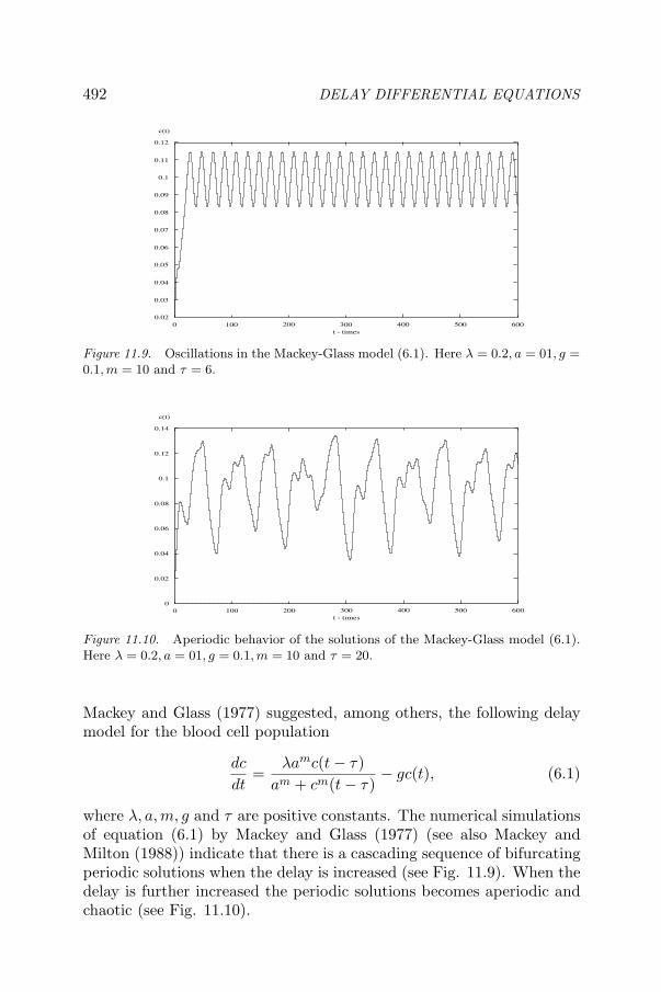
492 DELAY DIFFERENTIAL EQUATIONS
0.02
0.03
0.04
0.05
0.06
0.07
0.08
0.09
0.1
0.11
0.12
c(t)
0 100 200 300 400 500 600t - times
Figure 11.9. Oscillations in the Mackey-Glass model (6.1). Here λ = 0.2, a = 01, g =0.1, m = 10 and τ = 6.
0
0.02
0.04
0.06
0.08
0.1
0.12
0.14
c(t)
0 100 200 300 400 500 600t - times
Figure 11.10. Aperiodic behavior of the solutions of the Mackey-Glass model (6.1).Here λ = 0.2, a = 01, g = 0.1, m = 10 and τ = 20.
Mackey and Glass (1977) suggested, among others, the following delaymodel for the blood cell population
dc
dt=
λamc(t − τ)am + cm(t − τ)
− gc(t), (6.1)
where λ, a, m, g and τ are positive constants. The numerical simulationsof equation (6.1) by Mackey and Glass (1977) (see also Mackey andMilton (1988)) indicate that there is a cascading sequence of bifurcatingperiodic solutions when the delay is increased (see Fig. 11.9). When thedelay is further increased the periodic solutions becomes aperiodic andchaotic (see Fig. 11.10).

DDE in Single Species Dynamics 493
6.2 Wazewska-Czyzewska and Lasota ModelAnother well-known model belongs to Wazewska-Czyzewska and La-
sota (1976) which takes the form
dN
dt= −µN(t) + pe−γN(t−τ), (6.2)
where N(t) denotes the number of red-blood cells at time t, µ is theprobability of death of a red-blood cell, p and γ are positive constantsrelated to the production of red-blood cells per unit time and τ is thetime required to produce a red-blood cells. See also Arino and Kimmel(1986).
Global attractivity in the Mackey-Glass model (6.1) and the Lasota-Wazewska model (6.2) has been studied by Gopalsamy et al. (1990b),Karakostas et al. (1992), Kuang (1992) and Gyori and Trofimchuk(1999). Liz et al. (2002) study these models when the delay is infi-nite.
Other types of delay physiological models can be found in Mackeyand Milton (1988,1990) and Fowler and Mackey (2002).
7. A Vector Disease ModelLet y(t) denote the infected host population and x(t) be the popu-
lation of uninfected human. Assume that the total host population isconstant and is scaled so that
x(t) + y(t) = 1.
The disease is transmitted to the host by an insect vector, assumed tohave a large and constant population, and by the host to that vector.Within the vector there is an incubation period τ before the diseaseagent can infect a host. So the population of vectors capable of infectingthe host is
z(t) = dy(t − τ).where d is the infective rate of the vectors. Infection of the host isassumed to proceed at a rate (e) proportional to encounters betweenuninfected host and vectors capable of transmitting the disease,
ex(t) · dy(t − τ) = by(t − τ)[1 − y(t)],
and recovery to proceed exponentially at a rate c. Thus, b is the contactrate. Infection leads neither to death, immunity or isolation. Based onthese assumptions, Cooke (1978) proposed a delay model
dy
dt= by(t − τ)[1 − y(t)] − ay(t), (7.1)
where a > 0 is the cure rate.

494 DELAY DIFFERENTIAL EQUATIONS
0
0.05
0.1
0.15
0.2
0.25
0.3
0.35
0.4
0.45
0.5
u(t)
0 10 20 30 40 50 60t - time
a>b
a<b
Figure 11.11. Numerical simulations for the vector disease equation (7.1). Whena = 5.8, b = 4.8(a > b), the zero steady state u = 0 is asymptotically stable; Whena = 3.8, b = 4.8(a < b), the positive steady state u∗ is asymptotically stable for alldelay values; here for both cases τ = 5.
Using the Liapunov functional method, he obtained the following re-sults on global stability of the steady states.
Theorem 5 For the vector disease model ( 7.1), we have the following:
(i) If 0 < b ≤ a, then the steady state solution u0 = 0 is asymptoticallystable and the set φ ∈ ([−τ, 0], R) : 0 ≤ φ(θ) ≤ 1 for − τ ≤ θ ≤0 is a region of attraction.
(ii) If 0 ≤ a < b, then the steady state solution u1 = (b − a)/b isasymptotically stable and the set φ ∈ ([−τ, 0], R) : 0 < φ(θ) ≤1 for − τ ≤ θ ≤ 0 is a region of attraction.
The stability results indicate that there is a threshold at b = a. Ifb ≤ a, then the proportion u of infectious individuals tends to zero ast becomes large and the disease dies out. If b > a, the proportion ofinfectious individuals tends to an endemic level u1 = (b − a)/b as tbecomes large. There is no non-constant periodic solutions in the region0 ≤ u ≤ 1. Numerical simulations are given in Fig. 11.11.
Busenberg and Cooke (1978) studied the existence of periodic solu-tions in the vector-host model (7.1) when b = b(t) is a positive periodicfunction.

DDE in Single Species Dynamics 495
8. Multiple DelaysKitching (1977) pointed out that the life cycle of the Australian
blowfly Lucila cuprina has multiple time delay features which need tobe considered in modelling its population. Based on this observation,Braddock and van den Driessche (1983) proposed the two delay logisticequation (see also Gopalsamy (1990))
dx
dt= rx(t)[1 − a1x(t − τ1) − a2x(t − τ2)], (8.1)
where r, a1, a2, τ1 and τ2 are positive constants. Other equations withtwo delays appear in neurological models (Belair and Campbell (1994)),physiological models (Beuter et al. (1993)), medical models (Belair etal. (1995)), epidemiological models (Cooke and Yorke (1973)), etc. Veryrich dynamics have been observed in such equations (Hale and Huang(1993), Mahaffy et al. (1995)).
Equation (8.1) has a positive equilibrium x∗ = 1/(a1 +a2). Let x(t) =x∗(1 + X(t)). Then (8.1) becomes
X(t) = −(1 + X(t))[A1X(t − τ1) + A2X(t − τ2)], (8.2)
where A1 = ra1x∗, A2 = ra2x
∗. The linearized equation of (8.2) at X = 0is
X(t) = −A1X(t − τ1) − A2X(t − τ2).
Braddock and van den Driessche (1983) described some linear stabilityregions for equation (8.1) and observed stable limit cycles when τ2/τ1 islarge. Gopalsamy (1990) obtained stability conditions for the positiveequilibrium. Using the results in Li et al. (1999), we can obtain thefollowing theorem on the stability and bifurcation of equation (8.1).
Theorem 6 If one of the following conditions is satisfied:
(i) A1 < A2 and τ1 > 0 such that π2τ1
<√
A22 − A2
1 < 3π2τ1
;
(ii) A2 < A1 and τ1 > π2(A1+A2) such that τ1 ∈ [ π
2(A1+A2) , τ1], where
τ1 = (A21 − A2
2)− 1
2 arcsin√
(A21 − A2
2)/A21;
(iii) A1 = A2 and τ1 > 12A1
;
then there is a τ02 > 0, such that when τ2 = τ0
2 the two-delay equation( 8.1) undergoes a Hopf bifurcation at x∗ = 1/(a1 + a2).

496 DELAY DIFFERENTIAL EQUATIONS
0.6
0.8
1
1.2
1.4
1.6
x(t)
0 50 100 150 200t - time
(a)
(b)
Figure 11.12. For the two delay logistic model (8.1), choose r = 0.15, a1 = 0.25, a2 =0.75. (a) The steady state (a) is stable when τ1 = 15 and τ2 = 5 and (b) becomesunstable when τ1 = 15 and τ2 = 10, a Hopf bifurcation occurs.
Lenhart and Travis (1986) studied the global stability of the multipledelay population model
dx
dt= x(t)
[r + ax(t) +
n∑i=1
bix(t − τi)
]. (8.3)
Their global stability conditions very much depend on the negative, in-stantaneously dominated constant a. It would be interesting to deter-mine the dynamics of the multiple-delay logistic equation without thenegative instantaneously dominated term (see Kuang (1993))
dx
dt= rx(t)
[1 −
n∑i=1
x(t − τi)Ki
]. (8.4)
9. Volterra Integrodifferential EquationsThe Hutchinson’s equation (2.1) means that the regulatory effect de-
pends on the population at a fixed earlier time t − τ , rather than atthe present time t. In a more realistic model the delay effect shouldbe an average over past populations. This results in an equation witha distributed delay or an infinite delay. The first work using a logisticequation with distributed delay was by Volterra (1934) with extensionsby Kostitzin (1939). In the 1930’s, many experiments were performedwith laboratory populations of some species of small organisms withshort generation time. Attempts to apply logistic models to these ex-periments were often unsuccessful because populations died out. One of

DDE in Single Species Dynamics 497
the causes was the pollution of the closed environment by waste prod-ucts and dead organisms. Volterra (1934) used an integral term or adistributed delay term to examine a cumulative effect in the death rateof a species, depending on the population at all times from the start ofthe experiment. The model is an integro-differential equation
dx
dt= rx
[1 − 1
K
∫ t
−∞G(t − s)x(s)dx
], (9.1)
where G(t), called the delay kernel, is a weighting factor which indi-cates how much emphasis should be given to the size of the populationat earlier times to determine the present effect on resource availability.Usually the delay kernel is normalized so that
∫ ∞
0G(u)du = 1.
In this way we ensure that for equation (9.1) the equilibrium of theinstantaneous logistic equation (1.3) remains an equilibrium in the pres-ence of time delay. If G(u) is the Dirac function δ(τ − t), where
∫ ∞
−∞δ(τ − s)f(s)ds = f(τ),
then equation (9.1) reduces to the discrete delay logistic equation
dx
dt= rx(t)
[1 − 1
K
∫ t
−∞δ(t − τ − s)x(s)dx
]= rx(t)
[1 − x(t − τ)
K
].
The average delay for the kernel is defined as
T =∫ ∞
0uG(u)du.
It follows that if G(u) = δ(u − τ), then T = τ , the discrete delay. Weusually use the Gamma distribution delay kernel
G(u) =αnun−1e−αu
(n − 1)!, n = 1, 2, . . . (9.2)
where α > 0 is a constant, n an integer, with the average delay T = n/α.Two special cases,
G(u) = αe−αu (n = 1), G(u) = α2ue−αu; (n = 2),
are called weak delay kernel and strong delay kernel, respectively. Theweak kernel qualitatively indicates that the maximum weighted response
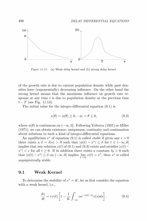
498 DELAY DIFFERENTIAL EQUATIONS
Figure 11.13. (a) Weak delay kernel and (b) strong delay kernel.
of the growth rate is due to current population density while past den-sities have (exponentially) decreasing influence. On the other hand thestrong kernel means that the maximum influence on growth rate re-sponse at any time t is due to population density at the previous timet − T (see Fig. 11.13).
The initial value for the integro-differential equation (9.1) is
x(θ) = φ(θ) ≥ 0,−∞ < θ ≤ 0, (9.3)
where φ(θ) is continuous on (−∞, 0]. Following Volterra (1931) or Miller(1971), we can obtain existence, uniqueness, continuity and continuationabout solutions to such a kind of integro-differential equations.
An equilibrium x∗ of equation (9.1) is called stable if given any ε > 0there exists a δ = δ(ε) > 0 such that |φ(t) − x∗| ≤ δ for t ∈ (−∞, 0]implies that any solution x(t) of (9.1) and (9.3) exists and satisfies |x(t)−x∗| < ε for all t ≥ 0. If in addition there exists a constant δ0 > 0 suchthat |φ(t) − x∗| ≤ δ on (−∞, 0] implies lim
t→∞x(t) = x∗, then x∗ is called
asymptotically stable.
9.1 Weak Kernel
To determine the stability of x∗ = K, let us first consider the equationwith a weak kernel, i.e.,
dx
dt= rx(t)
[1 − 1
K
∫ t
−∞αe−α(t−s)x(s)ds
]. (9.4)
T u
α
0
(a) (b)
0u

DDE in Single Species Dynamics 499
Using the linear chain trick (Fargue (1973) and MacDonald (1978)),define
y(t) =∫ t
−∞αe−α(t−s)x(s)ds. (9.5)
Then the scalar integro-differential equation (9.4) is equivalent to thefollowing system of two ordinary differential equations
dxdt
= rx(t)[1 − 1
K y(t)],
dydt
= αx(t) − αy(t).(9.6)
Notice that the positive equilibrium of system (9.6) is (x∗, y∗) = (K, K).To determine the stability of (x∗, y∗), let X = x − x∗, Y = y − y∗. Thecharacteristic equation of the linearized system is given by
λ2 + αλ + αr = 0, (9.7)
which has rootsλ1,2 = −α
2± 1
2
√α2 − 4αr.
Therefore, Reλ1,2 < 0, which implies that x∗ = K is locally asymptoti-cally stable.
In fact, x∗ = K is globally stable. Rewrite (9.1) as follows:
dxdt
= − rK x(t)(y(t) − y∗),
dydt
= α(x(t) − x∗) − α(y(t) − y∗).(9.8)
Choose a Liapunov function as follows
V (x, y) = x − x∗ − x∗ lnx
x∗ +r
2αK(y − y∗)2. (9.9)
Along the solutions of (9.8), we have
dV
dt=
dx
dt
x − x∗
x+
r
αK(y − y∗)
dy
dt= − r
K(y − y∗)2 < 0.
Since the positive quadrant is invariant, it follows that solutions of sys-tem (9.8), and hence of (9.1), approach (x∗, y∗) as t → ∞. Therefore,x(t) → x∗ as t → ∞.
The above analysis can be summarized as the following theorem.
Theorem 7 The positive equilibrium x∗ = K of the logistic equation( 9.1) with a weak kernel is globally stable (see Fig. 11.14).

500 DELAY DIFFERENTIAL EQUATIONS
0.2
0.4
0.6
0.8
1
1.2
x(t)
0 50 100 150 200t - time
alpha=0.125
alpha=1.25
Figure 11.14. The steady state of the integrodifferential equation (9.1) is globallystable. Here r = 0.15, K = 1.00.
The result indicates that if the delay kernel is a weak kernel, the logis-tic equation with distributed delay has properties similar to the instan-taneous logistic equation. We shall see that the logistic equation witha strong kernel exhibits richer dynamics similar to the logistic equationwith a constant delay.
9.2 Strong KernelConsider the logistic equation (9.1) with a strong kernel, i.e.,
dx
dt= rx(t)
[1 − 1
K
∫ t
−∞α2(t − s)e−α(t−s)x(t − s)ds
]. (9.10)
To use the linear chain trick, define
y(t) =∫ t
−∞αe−α(t−s)x(s)dx, z(t) =
∫ t
−∞α2(t − s)e−α(t−s)x(s)ds.
Then equation (9.10) is equivalent to the system
dxdt
= rx(t)(1 − 1
K z(t)),
dydt
= αx(t) − αy(t),
dzdt
= αy(t) − αz(t),
(9.11)
which has a positive equilibrium (x∗, y∗, ε∗) = (K, K, K). Consideringthe linearization of (9.11) at (x∗, y∗, z∗), we obtain the characteristicequation
λ3 + a1λ2 + a2λ + a3 = 0, (9.12)

DDE in Single Species Dynamics 501
wherea1 = 2α, a2 = α2, a3 = rα2.
The Routh-Hurwitz criterion says that all roots of the equation (9.12)have negative real parts if and only if the following inequalities hold:
a1 > 0, a3 > 0, a1a2 − a3 > 0. (9.13)
Clearly, a1 = 2α > 0, a3 = rα2 > 0. The last inequality becomes
α >r
2. (9.14)
Thus, the equilibrium x∗ = K is stable if α > r/2 and unstable ifα < r/2. Note that the average delay of the strong kernel is defined asT = 2/α. Inequality (9.14) then becomes
T <4r. (9.15)
Therefore, the equilibrium x∗ = K is stable for “short delays” (T < 4/r)and is unstable for “long delays” (T > 4/r).
When T = T0 = 4/r, (9.12) has a negative real root λ1 = −r and apair of purely imaginary roots λ2,3 = ±i r
2 . Denote by
λ(T ) = µ(T ) + iν(T )
the complex eigenvalue of (9.12) such that u(T0) = 0, ν(T0) = r/2. Wecan verify that
dµ
dT
∣∣∣∣∣T= 4
r
=85r2 > 0. (9.16)
The transversality condition (9.16) thus implies that system (9.11) andhence equation (9.10) exhibits a Hopf bifurcation as the average delayT passes through the critical value T0 = 4/r (Marsden and McKraeken(1976)).
We thus have the following theorem regarding equation (9.10).
Theorem 8 The positive equilibrium x∗ = K of equation ( 9.10) is as-ymptotically stable if the average delay T = 2/α < 4/r and unstable ifT > 4/r. When T = 4/r, a Hopf bifurcation occurs at x∗ = K and afamily of periodic solutions bifurcates from x∗ = K, the period of thebifurcating solutions is π
ν0= 2π
r , and the periodic solutions exist forT > 4/r and are orbitally stable.
Thus, the logistic equation with a strong delay kernel, just like thelogistic equation with a discrete delay, exhibits a typical bifurcationphenomenon. As the (average) delay is increased through a critical valuethe positive equilibrium passes from stability to instability, accompaniedby the appearance of stable periodic solutions (see Fig. 11.15).

502 DELAY DIFFERENTIAL EQUATIONS
0
0.5
1
1.5
2
2.5
3
3.5
4
4.5
x(t)
0 50 100 150 200 250 300 350 400 450 500t - time
alpha=0.065
alpha=0.65
Figure 11.15. The steady state x∗ = K of the integrodifferential equation (9.10)losses stability and a Hopf bifurcation occurs when α changes from 0.65 to 0.065.Here r = 0.15, K = 1.00.
9.3 General KernelNow consider the stability of the equilibrium x∗ = K for the integrod-
ifferential equation (9.1) with a general kernel. Let X = x − K. Then(9.1) can be written as
dX
dt= −r
∫ t
−∞G(t − s)X(s)ds + rX(t)
∫ t
−∞G(t − s)X(s)ds.
The linearized equation about x = K is given by
dX
dt= −r
∫ t
−∞G(t − s)X(s)ds (9.17)
and the characteristic equation takes the form
λ + r
∫ ∞
0G(s)e−λsds = 0. (9.18)
If all eigenvalues of the characteristic equation (9.18) have negative realparts, then the solution X = 0 of (9.17), that is, the equilibrium x∗ = Kof (9.1), is asymptotically stable.
Theorem 9 If ∫ ∞
0sG(s)ds <
1r,
then x∗ = K of ( 9.1) is asymptotically stable.

DDE in Single Species Dynamics 503
Proof. Since the roots of (9.18) coincide with the zeros of the function
g(λ) = λ + r
∫ ∞
0G(s)e−λsds,
we may apply the argument principle to g(λ) along the contour Γ =Γ(a, ε) that constitutes the boundary of the region
λ| ε ≤ Reλ ≤ a, −a ≤ Im ≤ a, 0 < ε < a.
Since the zeros of g(λ) are isolated, we may choose a and ε so thatno zeros of g(λ) lie on Γ. The argument principle now states that thenumber of zeros of g(λ) contained in the region bounded by Γ is equal tothe number of times g(λ) wraps Γ around the origin as λ traverses Γ. (Azero of g(λ) of multiplicity m is counted m times.) Thus, it suffices toshow for all small ε > 0 and all large a > r, that g(λ) does not encircle0 as λ traverses Γ(a, ε).
Along the segment of Γ given by λ = a + iν, −a ≤ µ ≤ a, we have
g(a + iν) = a + iν + r
∫ ∞
0G(s)e−(a+iν)sds.
Since a > 0, it follows that
∣∣∣∣∫ ∞
0G(s)e−(a+iν)sds
∣∣∣∣ ≤∫ ∞
0G(s)ds = 1.
Because a > r, we may conclude that every real value assumed by g(λ)along this segment must be positive. Along the segment of Γ given byλ = µ + ia, ε ≤ µ ≤ a, we have
g(µ + ia) = µ + ia + r
∫ ∞
0G(s)e−(µ+ia)sds.
A similar argument shows g(λ) to assume no real value along this path.In fact, Img(µ + ia) is always positive here. Similarly, one can showthat Img(µ − ia) is negative along the segment λ = µ − ia, ε ≤ µ ≤ a.By continuity, g(λ) must assume at least one positive real value (and nonegative values) as λ travels clockwise from ε + ia to ε − ia along Γ.
Finally, consider the path traced out as λ = ε + iν increases fromε − ia to ε + ia. Under the assumption, Img(ε + iν) is seen to increase

504 DELAY DIFFERENTIAL EQUATIONS
monotonically with ν. In fact,
d
dνImg(ε + iν) =
d
dν
[ν + r
∫ ∞
0G(s)e−εs sin(νs)ds
]
= 1 + r
∫ ∞
0sG(s)e−εs cos(νs)ds
≥ 1 − r
∫ ∞
0sG(s)ds
> 0.
It follows immediately that g(λ) assumes precisely one real value alongthis last segment of Γ. Since no zero of g(λ) lies on Γ, that real value isnon-zero. Assuming it to be negative, g(λ) would have wrapped Γ onceabout the origin, predicting exactly one zero λ0 of g(λ) inside the regionbounded by Γ. Since α and G are real, the zeros of g(λ) occur in complexconjugate pairs, forcing λ0 to be real. This, however, is a contradictionsince the positivity of α shows g(λ) to have no real positive zeros. Thus,the real value assumed by g(λ) along this last segment must be posi-tive. Therefore, g(λ) does not encircle the origin. This completes theproof.
9.4 RemarksIn studying the local stability of equation (9.1) with weak and strong
kernels, we applied the so-called linear chain trick to transform the scalarintergrodifferential equation into equivalent a system of first order or-dinary differential equations and obtained the characteristic equations(9.7) and (9.12). It should be pointed out that these characteristic equa-tions can be derived directly from the characteristic equation (9.18). IfG is a weak kernel, then (9.18) becomes
λ + r
∫ ∞
0αe−(λ+α)sds = λ +
αr
λ + α= 0,
which is equation (9.7). If G is a strong kernel, then (9.18) becomes
λ + r
∫ ∞
0α2se−(λ+α)sds = λ +
α2r
(λ + α)2= 0,
which is equation (9.12).One of the varieties of equation (9.1) is the following equation
dx
dt= x(t)
[a − bx(t) − c
∫ t
−∞G(t − s)x(s)ds
], (9.19)

DDE in Single Species Dynamics 505
where a > 0, b ≥ 0, c ≥ 0, b+c = 0. Stability and bifurcation of equation(9.19) have been studied by many researchers. We refer to Miller (1966),Cushing (1977a), MacDonald (1978) and references cited therein. SeeCorollary 13.
It should be pointed out that bifurcations can occur in equation (9.19)when other coefficients (not necessarily the average delay) are chosen asbifurcation parameters. For example, Landman (1980) showed that theexists a positive a∗ such that for a = a∗, a steady state becomes unstableand oscillatory solutions bifurcate for a near a∗. See also Simpson (1980).
10. PeriodicityIf the environment is not temporally constant (e.g., seasonal effects of
weather, food supplies, mating habits, etc.), then the parameters becometime dependent. It has been suggested by Nicholson (1933) that anyperiodic change of climate tends to impose its period upon oscillationsof internal origin or to cause such oscillations to have a harmonic relationto periodic climatic changes. Pianka (1974) discussed the relevance ofperiodic environment to evolutionary theory.
10.1 Periodic Delay ModelsNisbet and Gurney (1976) considered a periodic delay logistic equa-
tion and carried out a numerical study of the influence of the periodicityin r and K on the intrinsic oscillations of the equation such as thosecaused by the time delay. Rosen (1987) noted the existence of a relationbetween the period of the periodic carrying capacity and the delay ofthe logistic equation. Zhang and Gopalsamy (1990) assumed that theintrinsic growth rate and the carrying capacity are periodic functionsof a period ω and that the delay is an integer multiple of the period ofthe environment. Namely, they considered the periodic delay differentialequation of the form
dx
dt= r(t)x(t)
[1 − x(t − nω)
K(t)
], (10.1)
where r(t + ω) = r(t), K(t + ω) = K(t) for all t ≥ 0. They proved thefollowing result on the existence of a unique positive periodic solutionof equation (10.1) which is globally attractive with respect to all otherpositive solutions.
Theorem 10 Suppose that∫ nω
0r(s)ds ≤ 3
2. (10.2)

506 DELAY DIFFERENTIAL EQUATIONS
Then the periodic delay logistic equation ( 10.1) has a unique positivesolution x∗(t) and all other solutions of ( 10.1) corresponding to initialconditions of the form
x(θ) = φ(θ) ≥ 0, φ(0) > 0; φ ∈ C[−nω, 0]
satisfylimt→∞
|x(t) − x∗(t)| = 0. (10.3)
Following the techniques of Zhang and Gopalsamy (1990), quite a fewpapers have been produced by re-considering the delayed models whichappeared in the previous sections with the assumption that the coeffi-cients are periodic. See, for example, the periodic Nicholson’s blowfliesmodel (3.1) (Saker and Agarwal (2002)), the periodic Allee effect models(4.1)(Lalli and Zhang (1994)) and (4.2) (Yan and Feng (2003)), the pe-riodic food-limited model (5.3) (Gopalsamy et al. (1990a)), the periodicWazewska-Czyzewska and Lasota model (6.2) (Greaf et al. (1996)), etc.In all these papers, the delays are assumed to be integral multiples ofperiods of the environment. The coincidence degree theory (Gaines andMawhin (1977)) has also been used to establish the existence of peri-odic solutions in periodic models with general periodic delays. Howeveruniqueness is not guaranteed and stability can be obtained only whenthe delays are constant (Li (1998)).
Freedman and Wu (1992) considered the following single-species modelwith a general periodic delay
dx
dt= x(t)[a(t) − b(t)x(t) + c(t)x(t − τ(t))], (10.4)
where the net birth rate a(t) > 0, the self-inhibition rate b(t) > 0, thereproduction rate c(t) ≥ 0, and the delay τ(t) ≥ 0 are continuouslydifferentiable, ω-periodic functions on (−∞,∞). This model representsthe case that when the population size is small, growth is proportionalto the size, and when the population size is not so small, the positivefeedback is a(t) + c(t)x(t− τ(t)) while the negative feedback is b(t)x(t).Such circumstance could arise when the resources are plentiful and thereproduction at time t is by individuals of at least age τ(t) units of time.Using fixed point theorem and Razuminkin technique, they proved thefollowing theorem.
Theorem 11 Suppose that the equation
a(t) − b(t)K(t) + c(t)K(t − τ(t)) = 0
has a positive, ω-periodic, continuously differentiable solution K(t). Thenequation ( 10.4) has a positive ω-periodic solution Q(t). Moreover, if

DDE in Single Species Dynamics 507
b(t) > c(t)Q(t − τ(t))/Q(t) for all t ∈ [0, ω], then Q(t) is globally as-ymptotically stable with respect to positive solutions of ( 10.4).
Notice that in equation (10.4), b(t) has to be greater than zero. SoTheorem 11 does not apply to the periodic delay logistic equation
dx
dt= r(t)x(t)
[1 − x(t − τ(t))
K(t)
](10.5)
where τ(t) a positive periodic function. As Schley and Gourley (2000)showed, the periodic delays can have either a stabilizing effect or a desta-bilizing one, depending on the frequency of the periodic perturbation.It is still an open problem to study the dynamics, such as existence,uniqueness and stability of periodic solutions and bifurcations, for theperiodic delay logistic equation (10.5).
10.2 Integrodifferential EquationsPeriodic logistic equations with distributed delay have been systemati-
cally studied in Cushing (1977a). Bardi and Schiaffino (1982) consideredthe integrodifferential equation (9.1) when the coefficients are periodic,that is,
dx
dt= x(t)
[a(t) − b(t)x(t) − c(t)
∫ t
−∞G(t − s)x(s)ds
]. (10.6)
where a > 0, b > 0, c ≥ 0 are ω-periodic continuous functions on Rand G ≥ 0 is a normalized kernel. Let Cω = Cω(R, R) denote theBanach space of all ω-periodic continuous functions endowed with theusual supremum norm ‖x‖ = sup |x(t)|. For a ∈ Cω, define the averageof a as
〈a〉 =1ω
∫ ω
0a(s)ds.
The convolution of the kernel G and a bounded function f is defined by
(G ∗ f)(t) =∫ t
−∞G(t − s)f(s)ds.
Observe that an ω-periodic solution of (10.6) is a fixed point of theoperator B : Γ → Cω defined by
(Bx)(t) = u(t), t ∈ R,
where Γ = x ∈ Cω : 〈a − c(G ∗ x)〉 > 0. Since 〈a〉 > 0, x(t) ≡ 0belongs to Γ, that is, Γ is not empty. Define
u0(t) = (B0)(t).

508 DELAY DIFFERENTIAL EQUATIONS
Claim I. If x1 and x2 belong to Γ with x1 ≤ x2, then Bx2 ≤ Bx1.In fact, let αi(t) = a(t) − c(t)(G ∗ xi)(t) and ui(t) = (Bxi)(t) for
t ∈ R(i = 1, 2). Then α1(t) ≥ α2(t). Since αi(t) = ui(t)/ui(t)+ b(t)ui(t),we have 〈αi〉 = 〈bui〉 because ui(t)(i = 1, 2) are periodic. Thus, wededuce that 〈bu1〉 ≥ 〈bu2〉 and for some t0 ∈ R, u2(t0) ≤ u1(t0). Settingv(t) = u1(t) − u2(t), we have
v(t) ≥ (α1(t) − b(t)(u1(t) + u2(t)))v(t),
which implies that v(t) ≥ 0 for all t ≥ t0. By the periodicity of v(t), wehave Bx2 ≤ Bx1.
Claim II. If v and c belong to Cω, then 〈c(G ∗ v)〉 = 〈v(G ∗ c)〉.In fact, if we define G(t) = 0 for t < 0, we have
〈c(G ∗ v)〉 =+∞∑
j=−∞
∫ ω
0c(t)
∫ (j+1)ω
jωG(t − s)v(s)dsdt
=+∞∑
j=−∞
∫ ω
0c(t)
∫ ω
0G(t − s − jω)v(s)dsdt
=+∞∑
j=−∞
∫ ω
0v(t)
∫ (1−j)ω
−jωG(t − s)c(s)dsdt
= 〈v(G ∗ c)〉.
Claim III. Let z be a bounded continuous function on R. Then
lim inft→∞
(G ∗ z)(t) ≥ lim inft→∞
z(t); lim supt→∞
(G ∗ z)(t) ≤ lim supt→∞
z(t).
We only prove the first inequality. Let l = lim inft→∞ z(t). Chooseε > 0 and pick tε such that z(t) > l − ε for any t > tε. If t > tε, we have
(G ∗ z)(t) =∫ tε
−∞G(t − s)z(s)ds +
∫ t
tε
G(t − s)z(s)ds
≥ inft
z(t)∫ tε
−∞G(t − s)ds + (l − ε)
∫ t
tε
G(t − s)ds.
Hence,lim inft→∞
(G ∗ z)(t) ≥ l − ε,
which implies the first inequality.
Claim IV. Let u ∈ Γ and let v(t) > 0 be the solution of (10.6). Then
lim inft→∞
(v(t) − u(t)) > 0 implies lim inft→∞
((Bu)(t) − v(t)) > 0,
lim supt→∞
(v(t) − u(t)) < 0 implies lim supt→∞
(Bu)(t) − v(t)) < 0.

DDE in Single Species Dynamics 509
We prove the first statement. Let w(t) = (Bu)(t), t ∈ R. Then w(t)is a solution of
w(t) = a(t)w(t) − b(t)w(t)2 − c(t)w(t)(G ∗ u)(t)
whilev(t) = a(t)v(t) − b(t)v(t)2 − c(t)v(t)(G ∗ v)(t).
Define z(t) = w(t) − v(t). Then
z(t) = (a(t) − b(t)w(t) − c(t)(G ∗ u))z(t) + c(t)v(t)(G ∗ (v − u))(t)= (w(t)/w(t) − b(t)v(t))z(t) + c(t)v(t)(G ∗ (v − u))(t).
Let l = lim inft→∞(v(t) − u(t)). Because of Claim III, there exists at0 ∈ R, such that
z(t) > (w(t)/w(t) − b(t)v(t))z(t) + lc(t)v(t)/2
for all t > t0, that is,
z(t) > z(t0) exp∫ t
t0
β(s)ds +12
∫ t
t0
exp∫ t
sβ(θ)dθc(s)v(s)ds,
where β = w(t)/w(t) − b(t)v(t). Because w(t)/w(t) is periodic andits average is zero, b(t)v(t) is positive and bounded, we can see that∫ tt0
β(s)ds > γ1 − tγ2, where γ1 and γ2 > 0 are constants. Thus,
z(t) > γ3
∫ t
t0
exp((s − t)γ)ds = (γ3/γ)(1 − exp((t0 − t)γ2)),
where γ3 > 0 is a suitable constant. Then lim inft→∞ z(t) ≥ γ3/γ whichimplies the first statement.
Theorem 12 Suppose 〈a〉 > 0. If
b(t) > (G ∗ c)(t) (10.7)
for any t ∈ [0, ω], then equation ( 10.6) has a unique positive ω-periodicsolution x∗(t) which is globally asymptotically stable with respect to allsolutions of equation ( 10.6) under initial condition x(θ) = φ(θ), θ ∈(−∞, 0], φ(0) > 0.
Proof. Sinceu0(t)/u0(t) = a(t) − b(t)u0(t),
the periodicity of u0(t) and Claim II imply that 〈a〉 = 〈bu0〉 > 〈c(G∗u0)〉.As u0 > 0, we have Bu0 ≤ u0. Therefore, for any v ∈ Cω satisfying

510 DELAY DIFFERENTIAL EQUATIONS
0 < v ≤ u0, we have 0 < Bu0 ≤ Bv ≤ u0. Hence, the set Γ0 = v ∈ Cω :0 < v ≤ u0 ⊂ Γ is invariant under B. Moreover,
Bu0 ≤ Bv ≤ u0 ⇒ Bu0 ≤ B2v ≤ B2u0 ⇒ B3u0 ≤ B3v ≤ B2u0
and by induction
B2n+1u0 ≤ B2n+1v ≤ B2nu0, B2n+1u0 ≤ B2n+2v ≤ B2n+2u0, n = 0, 1, 2, ...
Since 0 < B20 = Bu0, by Claim I, we know that B2n+1u0 is in-creasing and B2nu0 is decreasing. Define
un(t) = (Bnu0)(t) = (Bun−1)(t).
Thenu−(t) = lim
n→∞u2n+1(t) and u+(t) = lim
n→∞u2n(t)
exist with 0 < u−(t) ≤ u+(t). If we can show that u−(t) = u+(t) = u∗(t),it is easy to see that u∗(t) is the unique fixed point of B. By the definition,we have
un(t) = (a(t) − c(t)(G ∗ un−1)(t))un(t) − b(t)un(t)2.
By the monotonicity and uniform boundedness of un we have theL2−convergence of both u2n+1 and u2n and their derivatives. Takingthe limits, we have
u−(t) = (a(t) − c(t)(G ∗ u+)(t))u−(t) − b(t)u−(t)2,u+(t) = (a(t) − c(t)(G ∗ u−)(t))u+(t) − b(t)u+(t)2.
Dividing them by u−(t) and u+(t) respectively, we have
〈a − c(G ∗ u+) − bu−〉 = 〈a − c(G ∗ u−) − bu+〉
followed by the fact that lnu+ and lnu− are periodic. Let v(t) = u+(t)−u−(t). Then we have 〈c(G ∗ v)〉 = 〈bv〉. Now by Claim II we have 〈c(G ∗v)〉 = 〈v(G ∗ c)〉. Hence, 〈v(b − G ∗ c)〉 = 0, which implies that v ≡ 0 bythe assumption (10.7). Therefore, u∗(t) is a unique periodic solution ofthe equation (10.6).
To prove the global stability, first we show that any solution v(t) ofequation (10.6) satisfies lim inft→∞ v(t) > 0. In fact, we have
v(t) < a(t)v(t) − b(t)v(t)2
andlim sup
t→∞(v(t) − (Bu)(t)) ≤ 0.

DDE in Single Species Dynamics 511
Choose ε > 0 so that u(t) = u0(t) + ε ∈ Γ. By Claim IV we have
lim inft→∞
(v(t) − (Bu)(t)) ≥ ε.
Since (Bu)(t) is strictly positive and periodic, we have lim inft→∞ v(t) >0. Thus, by Claim III, lim inft→∞(u0(t) − v(t)) > 0 and by induction,
lim inft→∞
(v(t) − (B2n+1u0)(t)) > 0, lim supt→∞
(v(t) − (B2nu0)(t)) < 0.
Given ε > 0, choose n such that
u∗(t) − ε < (B2n+1u0)(t) < (B2nu0)(t) < u∗(t) + ε.
Since (B2n+1u0)(t) < v(t) < (B2nu0)(t) for large t, it follows that thesequence Bju tends to u∗ uniformly as j → ∞.
If a, b and c are real positive constants, then condition (10.7) becomesb > c. This is the main result in Miller (1966).
Corollary 13 If b > c and G satisfies the above assumptions, then thepositive equilibrium x∗ = a/(b + c) of equation ( 9.19) (with constantcoefficient) is globally stable with respect to positive solutions of ( 9.19).
For other related work on periodic logistic equations with distributeddelay, we refer to Bardi (1983), Cohen and Rosenblat (1982), Cushing(1977a), Karakostas (1982) and the references therein.
11. State-Dependent DelaysLet x(t) denote the size of a population at time t. Assume that the
number of births is a function of the population size only. The birthrate is thus density dependent but not age dependent. Assume that thelifespan L of individuals in the population is variable and is a function ofthe current population size. If we take into account the crowding effects,then L(·) is a decreasing function of the population size.
Since the population size x(t) is equal to the total number of livingindividuals, we have (Belair (1991))
x(t) =∫ t
t−L[x(t)]b(x(s))ds. (11.1)
Differentiating with respect to the time t on both sides of equation(11.1) leads to a state-dependent delay model of the form
dx
dt=
b(x(t)) − b(x(t − L[x(t)])1 − L′[x(t)] b(x(t − L[x(t)])
. (11.2)

512 DELAY DIFFERENTIAL EQUATIONS
0.6
0.8
1
1.2
1.4
1.6
1.8
x(t)
0 50 100 150 200 250 300t - time
a=5
a=9.1541
Figure 11.16. Numerical simulations for the state-dependent delay model (11.3) withr = 0.15, K = 1.00 and τ(x) = a + bx2. (i) a = 5, b = 1.1; and (ii) a = 9.1541, b = 1.1.
Note that state-dependent delay equation (11.2) is not equivalent tothe integral equation (11.1). It is clear that every solution of (11.1) isa solution of (11.2) but the reverse is not true. In fact, any constantfunction is a solution of (11.2) but clearly it may not necessarily be asolution of (11.1). The asymptotic behavior of the solutions of (11.2)has been studied by Belair (1991). See also Cooke and Huang (1996).
State-dependent delay models have also been introduced by Kirk etal. (1970) to model the control of the bone marrow stem cell populationwhich supplies the circulating red blood cell population. See also Mackeyand Milton (1990).
Numerical simulations (see Fig. 11.16) show that the logistic modelwith a state-dependent delay
x′(t) = rx(t)[1 − x(t − τ(x(t))
K
], (11.3)
has similar dynamics to the Hutchinson’s model (2.1). Choose r =0.15, K = 1.00 as in Fig. 11.3 for the Hutchinson’s model (2.1) andτ(x) = a + bx2. We observe stability of the equilibrium x = K = 1 forsmall amplitude of τ(x) and oscillations about the equilibrium for largeamplitude of τ(x) (see Fig. 11.16).
Recently, great attention has been paid on the study of state-dependentdelay equations. Consider
εx′(t) = −x(t) + f(x(t − r(x(t)))) (11.4)
and assume that

DDE in Single Species Dynamics 513
(H1) A and B are given positive real numbers and f : [−B, A] →[−B, A] is a Lipschitz map with xf(x) < 0 for all x ∈ [−B, A], x =0;
(H2) For A and B in (H1), r : [−B, A] → R is a Lipschitz map withr(0) = 1 and r(u) ≥ 0 for all u ∈ [−B, A];
(H1′) B is a positive real number and r : [−B,∞) → R is a locally Lip-schitz map with r(0) = 1, r(u) ≥ 0 for all u ≥ −B and r(−B) = 0;
(H2′) f : R → R is a locally Lipschitz map, and if B is as in (H1′)and A = sup|f(u)| : −B ≤ u ≤ 0, then uf(u) < 0 for allu ∈ [−B, A], u = 0.
A periodic solution x(t) of (11.4) is called an slowly oscillating periodic(SOP) solution if there exist numbers q1 > 1 and q2 > q1 + 1 such that
x(t)
= 0, t = 0,< 0, 0 < t < q1,= 0, t = q1,> 0, q1 < t < q2,= 0, t = q2
and x(t+ q2) = x(t) for all t. Mallet-Paret and Nussbaum (1992) provedthe following theorem.
Theorem 14 Assume that f and r satisfy (H1)-(H2) or (H1′)-(H2′).Suppose that f is in C1 near 0 and f ′(0) = −k < −1. Let ν0, π/2 < ν0 <π, be the unique solution of cos ν0 = −1/k and define λ0 = ν0/
√k2 − 1.
Then for each λ > λ0 the equation
x′(t) = −λx(t) + λf(x(t − r(x(t))))
has an SOP solution xλ(t) such that −B < xλ(t) < A for all t.
Mallet-Paret and Nussbaum (1996, 2003) studied the shape of generalperiodic solutions of the equation (11.4) and their limiting profile asε → 0+. We refer to Arino et al. (1998), Bartha (2003), Kuang andSmith (1992a, 1992b), Mallet-Paret et al. (1994), Magal and Arino(2000), Walther (2002) for existence of periodic solutions; to Krisztinand Arino (2001) for the existence of two dimensional attractors; toLouihi et al. (2002) for semigroup property of the solutions; to Bartha(2001) and Chen (2003) for convergence of solutions, and to Ait Dadsand Ezzinbi (2002) and Li and Kuang (2001) for almost periodic andperiodic solutions to state-dependent delay equations. See also Arino etal. (2001) for a brief review on state-dependent delay models.

514 DELAY DIFFERENTIAL EQUATIONS
12. Diffusive Models with DelayDiffusion is a phenomenon by which a group of particles, for example
animals, bacteria, cells, chemicals and so on, spreads as a whole ac-cording to the irregular motion of each particle. When this microscopicirregular movement results in some macroscopic regular motion of thegroup, the phenomenon is a diffusion process. In terms of randomness,diffusion is defined to be a basically irreversible phenomenon by whichparticles spread out within a given space according to individual randommotion.
12.1 Fisher EquationLet u(x, t) represent the population density at location x and time t
and the source term f represents the birth-death process. With the logis-tic population growth f = ru(1−u/K) where r is the linear reproductionrate and K the carrying capacity of the population, the one-dimensionalscalar reaction-diffusion equation takes the form (Fisher (1937) and Kol-mogorov et al. (1937))
∂u
∂t= D
∂2u
∂x2+ ru
(1 − u
K
), a < x < b, 0 ≤ t < ∞, (12.1)
which is called the Fisher equation or diffusive logistic equation. Fisher(1937) proposed the model to investigate the spread of an advantageousgene in a population.
Recall that for the spatially uniform logistic equation
∂u
∂t= ru
(1 − u
K
),
the equilibrium u = 0 is unstable while the positive equilibrium u = K isglobally stable. How does the introduction of the diffusion affect theseconclusions? The answer depends on the domain and the boundaryconditions. (a) In a finite domain with zero-flux (Neumann) boundaryconditions, the conclusions still hold (Fife (1979) and Britton (1986)).(b) Under the Dirichlet conditions, u = K is no longer a solution to theproblem. In this case the behaviour of solutions depends on the size ofthe domain. When the domain is small, u = 0 is asymptotically stable,but it losses its stability when the domain exceeds a certain size and anon-trivial steady-state solution becomes asymptotically stable. (c) Inan infinite domain the Fisher equation has travelling wave solutions (seeFigure 11.17).

DDE in Single Species Dynamics 515
0
0.2
0.4
0.6
0.8
1
u(x,t)
0 5 10 15 20z=x-ct
Figure 11.17. The traveling front profiles for the Fisher equation (12.1). Here D =r = K = 1, c = 2.4 − 3.0
12.2 Diffusive Equations with DelayIn the last two decades, diffusive biological models with delays have
been studied extensively and many significant results have been estab-lished. For instance, the diffusive logistic equations with a discrete delayof the form
∂u(x, t)∂t
= D∂2u(x, t)
∂x2+ ru(x, t)
(1 − u(x, t − τ)
K
)(12.2)
with either Neumann or Dirichlet boundary conditions have been investi-gated by Green and Stech (1981), Lin and Khan (1982), Yoshida (1982),Morita (1984), Luckhaus (1986), Busenberg and Huang (1996), Feng andLu (1996), Huang (1998), Freedman and Zhao (1997), Faria and Huang(2002), etc. The diffusive logistic equations with a distributed delay ofthe form
∂u(x, t)∂t
= D∂2u(x, t)
∂x2+ ru(x, t)
[1 − 1
K
∫ t
−∞G(t − s)u(x, t − s)ds
]
(12.3)have been studied by Schiaffino (1979), Simpson (1980), Tesei (1980),Gopalsamy and Aggarwala (1981), Schiaffino and A. Tesei (1981), Ya-mada (1993), Bonilla and Linan (1984), Redlinger (1985), Britton (1990),Gourley and Britton (1993), Pao (1997), etc.
Recently, researchers have studied the combined effects of diffusionand various delays on the dynamics of the models mentioned in previoussections. For example, for the food-limited model (5.3) with diffusion,Gourley and Chaplain (2002) considered the case when the delay is finite.

516 DELAY DIFFERENTIAL EQUATIONS
Feng and Lu (2003) assumed that the time delay in an integral multipleof the period of the environment and considered the existence of periodicsolutions. Davidson and Gourley (2001) studied the model with infinitedelay, and Gourley and So (2002) investigated the dynamics when thedelay is nonlocal.
The diffusive Nicholson’s blowflies equation
∂u
∂t= d∆u − τu(x, t) + βτu(x, t − 1) exp[−u(x, t − 1)] (12.4)
with Dirichlet boundary conditions has been investigated by So and Yang(1998). They studied the global attractivity of the positive steady stateof the equation. Some numerical and bifurcation analysis of this modelhas been carried out by So, Wu and Yang (1999) and So and Zou (2001).
Gourley and Ruan (2000) studied various local and global aspects ofNicholson’s blowflies equation with infinite delay
∂u
∂t= d∆u−τu(x, t)+βτ
(∫ t
−∞F (t − s)u(x, s) ds
)exp
(−∫ t
−∞F (t − s)u(x, s) ds
)
(12.5)
for (x, t) ∈ Ω× [0,∞), where Ω is either all of Rn or some finite domain,and the kernel satisfies F (t) ≥ 0 and the conditions
∫ ∞
0F (t) dt = 1 and
∫ ∞
0t F (t) dt = 1. (12.6)
Gourley (2000) discussed the existence of travelling waves in equation(12.5).
Ruan and Xiao (2004) considered the diffusive integro-differentialequation modeling the host-vector interaction
∂u
∂t(t, x) = d∆u(t, x)−au(t, x)+b[1−u(t, x)]
∫ t
−∞
∫
ΩF (t−s, x, y)u(s, y)dyds, (12.7)
where u(t, x) is the normalized spatial density of infectious host at timet ∈ R+ in location x ∈ Ω, Ω is an open bounded set in RN (N ≤ 3), andthe convolution kernel F (t, s, x, y) is a positive continuous function inits variables t ∈ R, s ∈ R+, x, y ∈ Ω, which is normalized so that
∫ ∞
0
∫
ΩF (t, s, x, y)dyds = 1.
Ruan and Xiao (2004) studied the stability of the steady states andproved the following results.
DDE in Single Species Dynamics 517
Theorem 15 The following statements hold
(i) If 0 < b ≤ a, then u0 = 0 is the unique steady state solution of( 12.7) in
M = u ∈ E : 0 ≤ u(x) ≤ 1, x ∈ Ωand it is globally asymptotically stable in C((−∞, 0]; M).
(ii) If 0 ≤ a < b, then there are two steady state solutions in M :u0 = 0 and u1 = (b − a)/b, where u0 is unstable and u1 is globallyasymptotically stable in C((−∞, 0]; M).
Notice that when F (t, s, x, y) = δ(x− y)δ(t− s− τ), where τ > 0 is aconstant, and u does not depend on the spatial variable, then equation(12.7) becomes the vector disease model (7.1) and Theorem 15 reducesto Theorem 5 obtained by Cooke (1978).
When x ∈ (−∞,∞) and the kernel is a local strong kernel, i.e.
∂u
∂t= d∆u(t, x) − au(t, x) + b[1 − u(t, x)]
∫ t
−∞
t − s
τ2e−
t−sτ u(s, x)ds,
(12.8)where (t, x) ∈ R+ × Ω, the existence of traveling waves has been estab-lished.
Theorem 16 For any τ > 0 sufficiently small there exist speeds c suchthat the system ( 12.8) has a traveling wave solution connecting u0 = 0and u1 = (b − a)/b.
The existence of traveling front solutions show that there is a movingzone of transition from the disease-free state to the infective state.
We refer to the monograph by Wu (1996) for a systematic treatmentof partial differential equations with delay.
Acknowledgements. The author would like to thank StephenCantrell for comments and corrections on an earlier version of the pa-per.

Chapter 12
WELL-POSEDNESS, REGULARITY ANDASYMPTOTIC BEHAVIOUR OFRETARDED DIFFERENTIAL EQUATIONSBY EXTRAPOLATION THEORY
L. ManiarDepartment of Mathematics,Faculty of Sciences Semlalia,B.P. 2390, Marrakesh 40000, [email protected]
1. IntroductionConsider the following inhomogeneous non-autonomous retarded dif-
ferential equation
(IRDE)
x′(t) = Ax(t) + L(t)xt + f(t), t ≥ s,x(τ) = ϕ(τ − s), τ ∈ [s − r, s],
where A is a linear (unbounded) operator on a Banach space E, (L(t))t≥0is a family of bounded linear operators from the space C([−r, 0], E)into E, f : IR+ −→ E, and xt is the function defined on [−r, 0] byxt(θ) = x(t + θ), θ ∈ [−r, 0].
The equation (IRDE) has attracted many authors, and has beentreated by using different techniques and methods, we cite, for instance,[1, 3, 44, 63, 64, 105, 226, 227, 253]. In these papers, it has been stud-ied the well-posedness of the inhomogeneous autonomous retarded dif-ferential equations (IRDE) (L(t) ≡ L). It has been also studied theasymptotic behaviour and the regularity properties of the solutions ofhomogeneous retarded equations (HRDE) (f ≡ 0) as well as the asymp-totic behaviour of the solutions of the inhomogeneous equations withrespect to the inhomogeneous term f .
To profit from the big development of the semigroup theory and itstools (as the perturbation technique), many authors thought to trans-form the retarded equation (IRDE) to an abstract Cauchy problem (un-
© 2006 Springer.
519
O. Arino et al. (eds.), Delay Differential Equations and Applications, 519–538.

520 DELAY DIFFERENTIAL EQUATIONS
retarded equation) in a product Banach space X := E×C([−r, 0], E) asfollows
(CP )f
U ′(t) = AU(t) + B(t)U(t) +(
f(t)0
), t ≥ s,
U(s) =(
0ϕ
),
where,
A :=(
0 Aδ0 − δ′00 d
dτ
),
D(A) := 0 ×φ ∈ C1([−r, 0], E) : φ(0) ∈ D(A)
,
and
B(t) :=(
0 L(t)0 0
), t ≥ 0.
The first remark that one can do is that X0 := D(A) = 0×C([−r, 0], E)= X , which means that the operator A is not densely defined. One re-marks also that the ranges of the perturbation operators B(t), t ≥ 0,
and the values of the inhomogeneous term(
f(t)0
), t ≥ 0, are not in
X0. Hence, one cannot use the standard theory of semigroups to solveneither the perturbation problem (CP)0 nor the inhomogeneous Cauchyproblem (CP)f .
H. R. Thieme [224], has showed the existence of mild solutions of theinhomogeneous autonomous Cauchy problem (CP)f , and then the onesof the inhomogeneous autonomous retarded equations, by the introduc-tion of a new variation of constants formula.
To study the well-posedness of the homogeneous non-autonomous re-tarded differential equations (HRDE), A. Rhandi [199] has proposed theuse of the so-called extrapolation theory, introduced by R. Nagel [63].Using the extrapolation theory, we have also treated, with A. Rhandi,[178] the well-posedness of the inhomogeneous autonomous retardedequations and, together with A. Batkai, [17], we studied the regular-ity of the solutions to the homogeneous autonomous equations. With B.Amir [8, 9, 10], also using the extrapolation theory, we have studied theasymptotic behaviour of solutions to the inhomogeneous autonomousretarded equations. Usually by the extrapolation theory, G. Guhring,F. Rabiger and R. Schnaubelt have studied [55, 92, 94, 93] the well-posedness and the asymptotic behaviour of the general inhomogeneousnon-autonomous retarded equations (IRDE).
Our contribution in this book consists in the study of the well-posedeness, the regularity and the asymptotic behaviour of the solu-

Extrapolation theory for DDE 521
tions of the homogeneous non-autonomous retarded differential equa-tions (HRDE), using the extrapolation theory. Our document is orga-nized as follows:
In section 2, we recall some definitions and important results from theextrapolation theory. More precisely, we define the extrapolation spacesand the extrapolated semigroups for Hille-Yosida operators, introducedby R. Nagel [63], and present some of their important properties. Atthe end, we present a perturbation of Hille-Yosida operators result, theresult is shown in [187, 199].
Section 3 is devoted to the application of the above abstract results, tostudy the homogeneous non-autonomous retarded differential equations(HRDE). We study the existence of solutions, and that these solutionsare given by Dyson-Phillips expansions and satisfy variation of constantsformulas. These last results will be crucial to study the regularity andthe asymptotic properties of these solutions.
2. PreliminariesIn this section we introduce the extrapolation spaces and extrapolated
semigroups and give all needed abstract results of the extrapolation the-ory, e.g., perturbation results. For more details we refer to the book[63] and [17, 186]. The extrapolation theory was introduced by R. Nagel[63, 186], and was successfully used in these last years for many purposes,see e.g., [6], [8], [92], [178], [186], [190], [199], [200] and [201].
We recall that a linear operator (A, D(A)) on a Banach space X iscalled a Hille-Yosida operator if there are constants M ≥ 1 and w ∈ R
such that
(w,∞) ⊂ ρ(A) and ‖(λ−w)nR(λ, A)n‖ ≤ M for all λ > w and n ∈ N.(2.1)
From the Hille-Yosida theorem, we have (cf. [109, Thm. 12.2.4]) the fol-lowing result.
Proposition 1 Let (A, D(A)) be a Hille-Yosida operator on a Banachspace X. Then, the part (A0, D(A0)) of A in X0 := (D(A), ‖ · ‖) given
The regularity results, presented in this section, have been also shownby many authors, using alternative different techniques, see, e.g., [1],[105], [226], [227] and [253], but the results concerning the asymptoticbehaviour are in our knowledge new.

522 DELAY DIFFERENTIAL EQUATIONS
by
D(A0) := x ∈ D(A) : Ax ∈ X0A0x := Ax for x ∈ D(A0)
generates a C0-semigroup (T0(t))t≥0 on X0. Moreover, we have ρ(A) =ρ(A0) and (λ−A0)−1 is the restriction of (λ−A)−1 to X0 for λ ∈ ρ(A).
Notice that Hille-Yosida operators on reflexive Banach spaces aredensely defined.
Proposition 2 Let (A, D(A)) be a Hille-Yosida operator on a reflexiveBanach space X. Then D(A) is dense in X and hence A generates aC0-semigroup .
As an immediate consequence of Proposition 2, we have
Corollary 3 Let (A, D(A)) be the generator of a C0-semigroup (T (t))t≥0
on a reflexive Banach space X. Then (A∗, D(A∗)) generates the C0-semigroup (T ∗(t))t≥0 on X∗.
From now on, (A, D(A)) will be a Hille-Yosida operator on a Banachspace X. We define on X0 the norm
‖x‖−1 := ‖R(λ0, A0)x‖, x ∈ X0,
for a fixed λ0 > ω. From the resolvent equation it is easy to see thatdifferent λ ∈ ρ(A) yield equivalent norms. The completion X−1 of X0
with respect to ‖ · ‖−1 is called the extrapolation space. The extrapolatedsemigroup (T−1(t))t≥0 is the unique continuous extension of (T0(t))t≥0
to X−1, since
‖T0(t)x‖−1 = ‖T0(t)R(λ0, A0)x‖ ≤ Meωt‖x‖−1, t ≥ 0, x ∈ X0.
It is strongly continuous and we denote by (A−1, D(A−1)) its generator.We have the following properties (see [186, Prop. 1.3, Thm. 1.4]).
Theorem 4 We have the following:
(a) ‖T−1(t)‖L(X−1) = ‖T0(t)‖L(X0), t ≥ 0.
(b) D(A−1) = X0.
(c) A−1 : X0 → X−1 is the unique continuous extension of A0.
(d) X is continuously embedded in X−1 and R(λ, A−1) is an extensionof R(λ, A) for λ ∈ ρ(A−1) = ρ(A).

Extrapolation theory for DDE 523
(e) A0 and A are the parts of A−1 in X0 and X, respectively.
(f) R(λ0, A−1)X0 = D(A0).
The following result, concerning the convolutions of (T−1(t))t≥0 andX-valued locally integrable functions, is one of the fundamental resultsof the extrapolation theory, and is the key to show the next theorem.For the proof, see [63].
Proposition 5 Let f ∈ L1loc(R+, X). Then,
(i) for all t ≥ s ≥ 0,∫ t
sT−1(t − r)f(r) dr ∈ X0 and
‖∫ t
sT−1(t − r)f(r) dr‖ ≤ M1
∫ t
seω(t−r)‖f(r)‖ dr, (2.2)
M1 is a constant independent of t and f . For contraction semigroups(T0(t))t≥0, M1 = 1 and ω = 0.
(ii) The function [0, +∞) t −→∫ t
0T−1(t − s)f(s)ds ∈ X0 is
continuous.
We end this section by a non-autonomous perturbation result of Hille-Yosida operators, due to A. Rhandi [199]. For the aim of this document,we need only a particular version of this result.
First, recall that a family (U(t, s))t≥s≥0 of bounded linear operatorson X is called evolution family if
(a) U(t, r)U(r, s) = U(t, s) and U(s, s) = Id for t ≥ r ≥ s ≥ 0 and
(b) (t, s) : t ≥ s ≥ 0 (t, s) → U(t, s)x is continuous for all x ∈ X.
Consider now a perturbation family B(·) ∈ Cb(R+,Ls(X0, X)), i.e.,B(t) ∈ L(X0, X) for all t ≥ 0, and t −→ B(t)x is a bounded continuousfunction on IR+ for all x ∈ X0.
For all t ≥ 0, let C(t) denote the part of the perturbed operatorA + B(t) in X0. By definition, the operator C(t) is defined by
C(t) = A + B(t), D(C(t)) = x ∈ D(A) : Ax + B(t)x ∈ X0.
The proof of the following perturbation result relies on the fundamen-tal Proposition 5.
Theorem 6 The expansion
U(t, s) =∞∑
n=0
Un(t, s), (2.3)

524 DELAY DIFFERENTIAL EQUATIONS
where
U0(t, s) := T0(t−s) and Un+1(t, s) :=∫ t
sT−1(t−σ)B(σ)Un(σ, s)dσ, n ≥ 0,
(2.4)converges in the uniform operator topology of L(X0) uniformly on com-pact subsets of (t, s) : t ≥ s ≥ 0 and defines an evolution family onX0, satisfying
‖U(t, s)‖ ≤ Me(ω+Mc)(t−s) (2.5)
for t ≥ s ≥ 0 and c := supτ≥0 ‖B(τ)‖L(X0,X).In addition, (U(t, s))t≥s≥0 satisfies the variation of constants formula
U(t, s)x = T0(t−s)x+∫ t
sT−1(t−σ)B(σ)U(σ, s)x dσ, x ∈ X0, t ≥ s ≥ 0.
(2.6)Moreover, if t −→ B(t)x is differentiable on IR+ for all x ∈ X0 then,for all x ∈ D(C(s)), t −→ U(t, s)x is differentiable on [s,∞), U(t, s)x ∈D(C(t)) and
d
dtU(t, s)x = (A + B(t))U(t, s)x
for all t ≥ s.In this case we say that the evolution family is generated by the family(C(t), D(C(t)))t≥0.
In the autonomous case, B(t) ≡ B, the operator
C = A + B, D(C) = x ∈ D(A) : Ax + Bx ∈ X0 (2.7)
generates a C0-semigroup (S(t))t≥0, see [187, Thm. 4.1.5]. From Theo-rem 6, the semigroup (S(t))t≥0 is given by the Dyson-Phillips expansion
S(t) =∞∑
n=0
Sn(t), (2.8)
S0(t) := T0(t) and Sn+1(t) :=∫ t
0T−1(t − σ)BSn(σ)dσ, t ≥ 0, n ≥ 0,
(2.9)and satisfies the variation of constants formula
S(t)x = T0(t)x +∫ t
0T−1(t − σ)BS(σ)xdσ, t ≥ 0, x ∈ X0. (2.10)

Extrapolation theory for DDE 525
3. Homogeneous Retarded DifferentialEquations
In this section we apply the extrapolation results from the previoussection to solve the homogeneous retarded differential equations
(HRDE)
x′(t) = Ax(t) + L(t)xt, t ≥ s,
xs = ϕ,
and study the regularity and the asymptotic behaviour of their solutions.Here, A is a Hille-Yosida operator on a Banach space E. Let S :=(S0(t))t≥0 the C0-semigroup generated by the part of A in E0 := D(A),and (S−1(t))t≥0 its extrapolated semigroup. (L(t))t≥0 is a family ofbounded linear operators from Cr := C([−r, 0], E0) to E.
By a (classical) solution of (HRDE), we design a continuously dif-ferentiable function x : [−r, +∞) −→ E0, which satisfies the equation(HRDE), and by a mild solution a continuous function x : [−r, +∞) −→E0, satisfying
x(t) =
S0(t − s)ϕ(0) +
∫ ts S−1(t − σ)L(σ)xσdσ, t ≥ s,
ϕ(t − s), s − r ≤ t ≤ s.
(3.1)To get the purpose of this section, we associate to the equation (HRDE)
an equivalent Cauchy problem on the product Banach space X := E×Cr
(CP )0
U ′(t) = A(t)U(t), t ≥ s,
U(s) =(
0ϕ
),
where, for every t ≥ 0,
A(t) :=(
0 Aδ0 − δ′0 + L(t)0 d
dτ
),
D(A(t)) := 0 ×φ ∈ C1([−r, 0], E0) : φ(0) ∈ D(A)
,
with δ0 is the mass of Dirac concentrated at 0, δ′0ϕ := ϕ
′(0) for all
ϕ ∈ C1([−r, 0] , E0).Before showing the equivalence of (HRDE) and (CP)0, we study the
well-posedness of the last Cauchy problem (CP)0. To do this, we writethe operator A(t) as the sum of the operator
A :=(
0 Aδ0 − δ′00 d
dτ
),

526 DELAY DIFFERENTIAL EQUATIONS
D(A) := 0 ×φ ∈ C1([−r, 0], E0) : φ(0) ∈ D(A)
,
and the operator
B(t) :=(
0 L(t)0 0
), t ≥ 0.
As we have remarked at the introduction, X0 := D(A) = 0×Cr whichmeans that the operator A is not densely defined. For this reason, wepropose to use the extrapolation theory to study the well-posedness ofthe Cauchy problem (CP)0.
To this purpose, we need to show that the operator A is of Hille-Yosida. This result has been shown in [199] when A generates a C0-semigroup.
Lemma 7 The operator A is of Hille-Yosida and
R (λ,A)n ( yg ) = ( 0
ϕn),
with
ϕn(τ) =
n−1∑i=0
eλτ (−τ)i
i!R(λ, A)n−i[y + g(0)] +
1
(n − 1)!
∫ 0
τ(σ − τ)n−1eλ(τ−σ)g(σ) dσ
(3.2)
for all τ ∈ [−r, 0], y ∈ E, g ∈ Cr and n ≥ 1.
Proof. From the equation (λ − A)( 0ϕ1
) = ( yg ) on the space X , we
have
ϕ1(τ) = eλτϕ1(0) +∫ 0
τeλ(τ−σ)g(σ) dσ, τ ∈ [−r, 0],
andAϕ1(0) − ϕ′
1(0) = y.
We conclude that
ϕ1(τ) = eλτR(λ, A)[y + g(0)] +∫ 0
τeλ(τ−σ)g(σ) dσ, τ ∈ [−r, 0].
It is clear that the function ϕ1 belongs to Cr, and the relation (3.2) issatisfied for n = 1. By induction, we obtain
ϕn(τ) =n−1∑i=0
eλτ (−τ)i
i!R(λ, A)n−i[y + g(0)] +
1(n − 1)!
∫ 0
τ(σ − τ)n−1eλ(τ−σ)g(σ) dσ, τ ∈ [−r, 0].
Since A is a Hille-Yosida operator, it follows that

Extrapolation theory for DDE 527
‖ϕn(τ)‖ ≤ M
(λ − ω)n‖y‖eλτ
n−1∑i=0
[(−λ + ω)τ ]i
i!+
‖g‖[ M
(λ − ω)neλτ
n−1∑i=0
[(−λ + ω)τ ]i
i!+
M
(n − 1)!∫ 0
τ(−σ)n−1eσ(λ−ω) dσ]
≤ M
(λ − ω)n[‖y‖ + ‖g‖].
The last inequality comes from
M
(λ − ω)n
n−1∑i=0
eλτ [(−λ + ω)τ ]i
i!+
M
(n − 1)!
∫ 0
τ(σ − τ)n−1e(λ−ω)(τ−σ) dσ =
M
(λ − ω)n
for τ ∈ [−r, 0]. Therefore,
‖R(λ,A)n‖ ≤ M
(λ − ω)nfor all λ > ω, n ≥ 1,
and this achieve the proof.The part of A in X0 is the operator
A0 =(
0 00 d
dτ
), D(A0) = 0 ×
φ ∈ C1([−r, 0], E0) : φ(0)
∈ D(A);ϕ′(0) = Aϕ(0)
,
and it generates a C0-semigroup (T0(t))t≥0, by Proposition 1. It is clearthen that the operator
A0 :=d
dτ, D(A0) :=
φ ∈ C1([−r, 0], E0) : φ(0) ∈ D(A);ϕ′(0) = Aϕ(0)
generates also a C0-semigroup (T0(t))t≥0, and one can easily show thatit is given by
(T0(t)ϕ) (θ) =
ϕ(t + θ), t + θ ≤ 0,
S0(t + θ)ϕ(0), t + θ > 0.(3.3)
Hence as A0 is a diagonal matrix operator, we have
T0(t) =(
I 00 T0(t)
), t ≥ 0.

528 DELAY DIFFERENTIAL EQUATIONS
To study now the existence of classical solution of (HRDE), we assume:(H) For all ϕ ∈ Cr, the function t −→ L(t)ϕ is continuously differen-
tiable.The linear operators B(t), t ≥ 0, are bounded from X0 into X and
from (H), the functions t −→ B(t)(
0ϕ
), ϕ ∈ Cr, are continuously dif-
ferentiable. Thus, by the perturbation result, Theorem 6, the family ofthe parts of operators (A + B(t)) in X0 generates an evolution family(U(t, s))t≥s≥0 on X0 given by the Dyson-Phillips expansion
U(t, s) =∞∑
n=0
Un(t, s), (3.4)
where
U0(t, s) := T0(t−s) and Un+1(t, s) :=∫ t
sT−1(t−σ)B(σ)Un(σ, s)dσ, n ≥ 0,
(3.5)and which satisfies the variation of constants formula
U(t, s)(
0ϕ
)=(
0T0(t−s)ϕ
)+∫ t
sT−1(t − σ)B(σ)U(σ, s)
(0ϕ
)dσ (3.6)
for all t ≥ s and ϕ ∈ Cr.One can see also that, for each t ≥ 0, the part of the operator
(A + B(t)) in X0 is the operator
(A + B(t))/X0=(
0 00 d
dτ
),
with the domain
D((A + B(t))/X0) = 0 ×
φ ∈ C1([−r, 0], E0) : φ(0) ∈ D(A);ϕ′(0)
= Aϕ(0) + L(t)ϕ .
Therefore, by identification of the elements of X0 and those of Cr, we getthe following result.
Proposition 8 Assume that (H) hold. The family (AL(t), D(AL(t)))t≥0of operators defined by
AL(t) :=d
dτ, D(AL(t)) : =
φ ∈ C1([−r, 0], E0) : φ(0) ∈ D(A);ϕ′(0)
= Aϕ(0) + L(t)ϕgenerates an evolution family (U(t, s))t≥s≥0 on the space , which sat-isfies the variation of constants formula
U(t, s)ϕ = T0(t−s)ϕ+ limλ→∞
∫ t
sT0(t − σ)eλ·λR(λ, A)L(σ)U(σ, s)ϕ dσ, t ≥ s, (3.7)
Cr

Extrapolation theory for DDE 529
and is given by the Dyson-Phillips series
U(t, s) =∞∑
n=0
Un(t, s), (3.8)
where
U0(t, s) = T0(t − s) and Un+1(t, s)
= limλ→∞
∫ t
s
T0(t − σ)eλ·λR(λ, A)L(σ)Un(σ, s)dσ, n ≥ 0, t ≥ s.(3.9)
Proof. As the operators (A + B(t))/X0, t ≥ 0, are diagonal matrix
operators on X0 = 0 × Cr, we can show that
U(t, s)(
0ϕ
)=(
0U(t,s)ϕ
)for all t ≥ s anϕ ∈ Cr,
and (U(t, s))t≥s≥0 is an evolution family on the space generated by(AL(t), D(AL(t)))t≥0.
By the variation of constants formula (3.6) and extrapolation results,we obtain that(
0U(t,s)ϕ
)=
(0
T0(t−s)ϕ
)+ lim
λ→∞λR (λ,A)
∫ t
sT−1(t − σ)B(σ)U(σ, s)
(0ϕ
)dσ
=(
0T0(t−s)ϕ
)+ lim
λ→∞
∫ t
sT0(t − σ)λR (λ,A)
(L(σ)U(σ,s)ϕ
0
)dσ.
Hence, by Lemma 7 we obtain the variation of constants formula (3.7).Also by the same argument, from the relations (3.4)-(3.5), we obtain
(3.8)-(3.8).
In the following proposition, we give the correspondence between themild solutions of the retarded equation (HRDE) and those of the Cauchyproblem (CP)0.
Proposition 9 Let ϕ ∈ Cr and s ≥ 0, we have:(i) The function defined by
x(t, s, ϕ) :=
ϕ(t − s), s − r ≤ t ≤ s,
U(t, s)ϕ(0), t > s,(3.10)
is the mild solution of (HRDE), i.e., x satisfies (3.1). Moreover, itsatisfies
U(t, s)ϕ = xt(·, s, ϕ), t ≥ s. (3.11)
Cr

530 DELAY DIFFERENTIAL EQUATIONS
(ii) If x(·, s, ϕ) is the mild solution of (HRDE) then t −→(
0xt(·,s,ϕ)
)
is the mild solution of the Cauchy problem (CP)0, and
xt(·, s, ϕ) = T0(t − s)ϕ + limλ→∞
∫ t
sT0(t − σ)eλ·λR(λ, A)L(σ)xσ(·, s, ϕ) dσ, t ≥ s.
Proof. Let τ ∈ [−r, 0] and ϕ ∈ Cr. From the extrapolation results, thevariation of constants formula (3.7) and the definition of (T0(t))t≥0, wehave
U(t, s)ϕ(τ) = T0(t − s)ϕ(τ) + limλ→∞
∫ t
sT0(t − σ)eλ·λR(λ, A)L(σ)U(σ, s)ϕ dσ(τ)
=
S0(t − s + τ)ϕ(0) + limλ→∞
∫ t+τ
sS0(t + τ − σ)λR(λ, A)L(σ)U(σ, s)ϕdσ+
+ limλ→∞
∫ t
t+τeλ(t+τ−s)λR(λ, A)L(σ)U(σ, s)ϕdσ if t − s + τ > 0,
ϕ(t − s + τ) + limλ→∞
∫ t
seλ(t+τ−s)λR(λ, A)L(σ)U(σ, s)ϕds if t − s + τ ≤ 0,
=
S0(t − s + τ)ϕ(0) +
∫ t+τ
sS−1(t + τ − σ)L(σ)U(σ, s)ϕdσ if t − s + τ > 0,
ϕ(t − s + τ) if t − s + τ ≤ 0
(3.12)
for all τ ∈ [−r, 0] and 0 ≤ s ≤ t. Let the function
x(t, s, ϕ) :=
ϕ(t − s), s − r ≤ t ≤ s,
U(t, s)ϕ(0), t > s.
Hence,
x(t, s, ϕ) = S0(t − s)ϕ(0) +∫ t−s
sS−1(t − σ)L(σ)U(σ, s)ϕdσ.
From the equality (3.12), one can obtain easily the relation (3.11).Thus, this implies that x(·, s, ϕ) satisfies (3.1), and the assertion (i) isproved. The assertion (ii) can also be deduced from the above relations.
In the particular case of autonomous retarded differential equations,i.e. L(t) = L for all t ≥ 0, we have the following theorem. The part (a)has been obtained also by many authors, e.g., [1], [63], [105] and [253].
Theorem 10 (a) The operator
AL :=d
dτ, D(AL) :=
ϕ ∈ C1([−r, 0], E0) : ϕ(0) ∈ D(A); ϕ′(0) = Aϕ(0) + Lϕ

Extrapolation theory for DDE 531
generates a strongly continuous C0-semigroup T := (T (t))t≥0 on thespace Cr.
Moreover, one has:(i) the solution x of (HRDE) is given by
x(t) :=
ϕ(t), −r ≤ t ≤ 0,
T (t)ϕ(0), t ≥ 0.(3.13)
(ii) If x is the solution of (HRDE), the semigroup T is given by
T (t)ϕ = xt for all ϕ ∈ Cr and t ≥ 0.
(b) The semigroup T is also given by the Dyson-Phillips series
T (t) =∞∑
n=0
Tn(t), t ≥ 0,
where
Tn(t)ϕ := limλ→∞
∫ t
0T0(t − s)eλ·λR(λ, A)LTn−1(s)ϕds,
or
Tn(t)ϕ(τ) =
∫ t+τ
0S−1(t + τ − s)LTn−1(s)ϕds if t + τ > 0,
0 if t + τ ≤ 0(3.14)
for all ϕ ∈ Cr and n ≥ 1, t ≥ 0.
Proof. The part of A + B in X0 = 0 × Cr is the operator given by
(A + B)/X0=
(0 0
0 ddτ
),
D((A + B)/X0) = 0 ×
φ ∈ C1([−r, 0], E0) : φ(0) ∈ D(A); ϕ′(0) = Aϕ(0) + Lϕ
.
From Section 2, the operator (A + B)/X0generates a C0-semigroup T :=
(T (t))t≥0. Hence, from the form of (A + B)/X0, one can see that the
operator (AL, D(AL)) generates also a C0-semigroup T := (T (t))t≥0 onCr, and
T (t) =(
I 00 T (t)
), t ≥ 0.
Moreover, T is given by the Dyson-Phillips series
T (t) =∞∑
n=0
Tn(t), t ≥ 0,

532 DELAY DIFFERENTIAL EQUATIONS
where
Tn(t)( 0ϕ ) := ( 0
Tn(t)ϕ ) :=∫ t
0T−1(t − s)BTn−1(s)( 0
ϕ ) ds, t ≥ 0.
From this and Lemma 7, one can see easily as in the non-autonomouscase that
Tn(t)ϕ = limλ→∞
∫ t
0T0(t − s)eλ·λR(λ, A)LTn−1(s)ϕds,
and from (3.3), for τ ∈ [−r, 0], we have
Tn(t)ϕ(τ) =
limλ→∞
∫ t+τ
0S0(t + τ − s)λR(λ, A)LTn−1(s)ϕds+
+ limλ→∞
∫ t
t+τeλ(t+τ−s)λR(λ, A)LTn−1(s)ϕds if t + τ > 0,
limλ→∞
∫ t
0eλ(t+τ−s)λR(λ, A)LTn−1(s)ϕds if t + τ ≤ 0.
Thus, we obtain the relation (3.14). The assertions (i)-(ii) are particularcases of Proposition 9.
The Dyson-Phillips series obtained in the above theorem will be nowused to study the regularity properties of the semigroup T solution of theretarded equation (HRDE). As, the terms Tn of the series, see (3.14),are convolutions between the extrapolated semigroup (S−1(t))t≥0 andE-valued functions, to get our aim, we need the following results.
Lemma 11 [17] Let G ∈ C(IR+,Ls(Cr)). Then,(i) If t : t > 0 t → S0(t) ∈ L(E0) is continuous (or S is
immediately norm continuous) then t : t > 0 t −→∫ t0 S−1(t −
s)LG(s) ds ∈ L(Cr, E0) is continuous.(ii) If the operator S0(t) is compact for all t > 0 (or S is immediately
compact) then the operator∫ t
0S−1(t − s)LG(s) ds
defined from Cr to E0 is compact for all t ≥ 0.
Now, we can announce the following regularity results, showed also,for instance, in [1], [63] and [253].
Theorem 12 (i) If S is immediately norm continuous then t : t >r t → T (t) ∈ L(Cr) is also a continuous function.(ii) If S is immediately compact then T (t) is also compact for all t > r.

Extrapolation theory for DDE 533
Proof. By the definition of the semigroup (T0(t))t≥0 it is easy toshow that t → T0(t) is norm continuous for t > r if we consider (i), andthat the operator T0(t) is compact for all t > r in the case of (ii).
Assume that S is immediately norm continuous. From the relations(3.14) and Lemma 11 (i), the function IR+ t → Tn(t) ∈ L(Cr) iscontinuous for all n ≥ 1. We have seen in Theorem 10 that
T (t) =∞∑
n=0
Tn(t) = T0(t) +∞∑
n=1
Tn(t), t ≥ 0, (3.15)
and that this series converge in L(Cr) uniformly in compact intervals ofIR+. Hence, the assertion (i) is obtained.
Treat now the assertion (ii). Let t > 0 and n ≥ 1. From Lemma 11,we have that ∫ t+θ
0S−1(t + θ − s)LTn−1(s) ds
is a compact operator from Cr to E0 for all t + θ ≥ 0, and then Tn(t)(θ)is also a compact operator from Cr to E0 for all θ ∈ [−r, 0].
By [63, Theorem II.4.29], we have also that S is immediately normcontinuous. Hence, by Lemma 11 (i), the set of functions θ →
∫ t+θ0 S−1(t+
θ−s)LTn−1(s)ϕds ϕ in some bounded set of Cr is equicontinuous, andthen the subset θ → Tn(t)(θ) ϕ in some bounded set of Cr of Cr isequicontinuous. The compactness of Tn(t) for all t > 0 and n ≥ 1follows finally from Arzela-Ascoli theorem. Consequently, as the series(3.15) converges in the uniform operator topology of Cr, we obtain thesecond assertion.
We end this section by studying the robustness of the asymptotic be-haviour of the solutions to non-autonomous retarded equation (HRDE)with respect to the term retard. More precisely, we show that thesolution of (HRDE) IR+ t −→ x(t) has the same asymptotic be-haviour, e.g., boundedness, asymptotic almost periodicity, as the mapIR+ t −→ S0(t)ϕ(0).
First, let us recall the following definitions:For a function f ∈ BUC(IR+, X0), the space of bounded and uni-
formly continuous functions from IR+ into X0, the set of all translates,called the hull of f , is H(f) := f(· + t) : t ∈ IR+.
The function f is said to be asymptotically almost periodic if H(f) isrelatively compact in BUC(IR+, X0), and Eberlein weakly asymptoticallyalmost periodic if H(f) is weakly relatively compact in BUC(IR+, X0),see [129] for more details.

534 DELAY DIFFERENTIAL EQUATIONS
A closed subspace E of BUC(IR+, X0) is said to be translation bi-invariant if for all t ≥ 0
f ∈ E ⇐⇒ f(· + t) ∈ E ,
and operator invariant if M f ∈ E for every f ∈ E and M ∈ L(X0),where M f is defined by (M f)(t) = M(f(t)), t ≥ 0.
The closed subspace E is said to be homogeneous if it is translationbi-invariant and operator invariant.
For our purpose, we assume that:(H1) the C0-semigroup (S0(t))t≥0 is of contraction,(H2) there exist s0 ≥ 0 and a constant 0 ≤ q < 1 such that
∫ ∞
0||L(s + t)T0(t)ϕ||dt ≤ q||ϕ|| for all ϕ ∈ Cr and s ≥ s0. (3.16)
Under the above hypotheses, we have the following results.
Proposition 13 (i) For all ϕ ∈ Cr, n ∈ N and t ≥ s ≥ s0
∫ +∞
s‖L(σ)Un(σ, s)ϕ‖dσ ≤ qn+1‖ϕ‖ (3.17)
and
‖Un(t, s)ϕ‖ ≤ qn‖ϕ‖. (3.18)
(ii) The series (3.8) converges uniformly on all the set (t, s) : t ≥ s ≥s0. Moreover, the evolution family (U(t, s))t≥s≥0 is uniformly boundedand
||U(t, s)|| ≤ 11 − q
for all t ≥ s ≥ s0.
Proof.Let ϕ ∈ Cr and t ≥ s ≥ s0. For n = 0, the estimate (3.17) is only
our assumption (3.16). Suppose now that the estimate holds for n − 1.From the relation (3.8), by using Fubini’s theorem we have

Extrapolation theory for DDE 535
∫ t
s||L(σ)Un(σ, s)ϕ||dσ
=∫ t
s||L(σ) lim
λ→∞
∫ σ
sT0(σ − τ)eλ·λR(λ, A)L(τ)Un−1(τ, s)ϕdτ‖ dσ
≤ limλ→∞
∫ t
s||∫ σ
sL(σ)T0(σ − τ)eλ·λR(λ, A)L(τ)Un−1(τ, s)ϕ‖dτ dσ
= limλ→∞
∫ t
s
∫ t−τ
0||L(σ + τ)T0(σ)eλ·λR(λ, A)L(τ)Un−1(τ, s)ϕ||dσdτ.
Hence, from (H1), the inequality (3.16) and the induction hypothesis∫ t
s||L(σ)Un(σ, s)ϕ||dσ ≤ q
∫ t
s‖L(τ)Un−1(τ, s)ϕ||dτ
≤ qn+1||ϕ||,
and this gives the estimate (3.17).The inequality (3.18) follows also from (H1), the relation (3.8) and
the first estimate (3.17).The assertion (ii) follows then by this estimate (3.18).
In the above proposition we obtain the boundedness of the evolutionfamily (U(t, s))t≥s≥0, and thus from (3.13), the boundedness of the mildsolution of (HRDE) is also obtained. To obtain the asymptotic almostperiodicity, and other asymptotic properties of this mild solution weneed the following Lemma.
Lemma 14 Let g ∈ L1(IR+, E). If t −→ T0(t)ϕ belongs to E for allϕ ∈ Cr then the function
IR+ t −→ T0 ∗ g(t) := limλ→∞
∫ t
0T0(t − τ)eλ·λR(λ, A)g(τ)dτ
belongs to E.
Proof. For g ∈ L1(IR+, E), since (T0(t))t≥0 is bounded, it is clear that∥∥∥∥ lim
λ→∞
∫ t
0T0(t − τ)eλ·λR(λ, A)g(τ)dτ
∥∥∥∥ ≤ C‖g‖L1 ,

536 DELAY DIFFERENTIAL EQUATIONS
which implies that for every g ∈ L1(IR+, E), T0∗g ∈ BC(IR+, Cr) and thelinear operator g −→ T0∗g is bounded from L1(IR+, E) into BC(IR+, Cr),the space of all bounded continuous functions. By this boundedness, thelinearity and the density, it is sufficient to show this result for simplefunctions. Let g := 1(a,b) ⊗ x, b ≥ a ≥ 0, x ∈ E and t ≥ 0. We have,
T0 ∗ g(t + b) = limλ→∞
∫ b
aT0(t + b − τ)eλ·λR(λ, A)x dτ
= T0(t) limλ→∞
∫ b
aT0(b − τ)eλ·λR(λ, A)x dτ.
Hence, since E is translation bi-invariant and t −→ T0(t)ϕ belongs toE for every ϕ ∈ Cr, we conclude that T0 ∗ g(·) ∈ E , and this achieve theproof.
We can now state the following main asymptotic behaviour result.
Theorem 15 Assume that (H1) and (H2) hold. If t −→ T0(t)ϕ be-longs to E for all ϕ ∈ Cr, and the condition ( 3.16) is satisfied then, theCr-valued function IR+ t −→ xt+s(·, s, ϕ) is also in E for all ϕ ∈ Cr
and s ≥ 0, where x(·, s, ϕ) is the mild solution of (HRDE).
Proof. From Proposition 9 and the relation (3.11), we have
xt+s(·, s, ϕ) = T0(t)ϕ+ limλ→∞
∫ t
0
T0(t − σ)eλ·λR(λ, A)L(s + σ)U(s + σ, s)ϕ dσ, t ≥ 0.
(3.19)
As t −→ T0(t)ϕ belongs to E , it is sufficient to that the function f fromIR+ to Cr
f(t) := limλ→∞
∫ t
0T0(t − σ)eλ·λR(λ, A)L(s + σ)U(s + σ, s)ϕdσ, t ≥ 0
belongs to E as well. Furthermore, by Lemma 14, it is sufficient to showthat the function g(·) := L(·+ s)U(·+ s, s)ϕ belongs to L1(IR+, E), andthis follows from (3.8) and the estimate (3.17) for all s ≥ s0. Hence,the function IR+ t −→ xt+s(·, s, ϕ) = U(t + s, s)ϕ belongs to E for alls ≥ s0 and ϕ ∈ Cr.
For all s ≥ 0 and t ≥ 0, one can write
U(t + s0 + s, s)ϕ = U(t + s + s0, s + s0)U(s + s0, s)ϕ.
As s + s0 ≥ s0, then as shown above t −→ U(t + s0 + s, s + s0)ϕ belongsto E and by the translation bi-invariance of E , t −→ xt+s(·, s, ϕ) =U(t + s, s)ϕ belongs to E . This achieves the proof.

Extrapolation theory for DDE 537
The C0-semigroup (T0(t))t≥0 is given in terms of the C0-semigroup(S0(t))t≥0, then we can hope that they have the same asymptotic be-haviour. In the following lemma, we present some particular communeasymptotic behaviours to these two semigroups.
Lemma 16 Let ϕ ∈ Cr. Assume that the map IR+ t −→ S0(t)ϕ(0) is(1) vanishing at infinity, or(2) asymptotically almost periodic, or
(3) uniformly ergodic, i.e., the limit limα→0+
α
∫ ∞
0e−αsS0(·+s)ϕ(0) ds ex-
ists and defines an element of BUC(IR+, E0), or
(4) totally uniformly ergodic, i.e., the Cesaro limit limt→+∞
1t
∫ t
0eiθsS0(·+
s)ϕ(0) ds exists in BUC(IR+, E0) for all θ ∈ IR.Then, the function IR+ t −→ T0(t)ϕ has the same property inBUC(IR+, Cr).
Proof.As (S0(t))t≥0 is a contraction semigroup, we have for all t > r and
θ ∈ [−r, 0]
‖(T0(t)ϕ)(θ)‖ = ‖S0(t + θ)ϕ(0)‖ = ‖S0(r + θ)S0(t − r)ϕ(0)‖≤ ‖S0(t − r)ϕ(0)‖.
If one has (1), then ‖T0(t)ϕ‖ −→ 0, when t → ∞.Assume now that we have (2). By the definition of asymptotic almost
periodicity, see [7], for every ε > 0 there is l(ε) > 0 and K ≥ 0 such thateach interval of length l(ε) contains a τ for which this inequality
||S0(t + τ)ϕ(0) − S0(t)ϕ(0)|| ≤ ε
holds for all t, t + τ ≥ K. Let now t > K + r. Then, one has
‖(T0(t + τ)ϕ)(θ) − (T0(t)ϕ)(θ)‖ = ‖S0(t + θ + τ)ϕ(0) − S0(t + θ)ϕ(0)‖≤ ‖S0(t − r + τ)ϕ(0) − S0(t − r)ϕ(0)‖< ε for all θ ∈ [−r, 0],
and this means that T0(·)ϕ is asymptotically almost periodic.The assertions (3) and (4) can be showed by the same technique.
As the classes of functions (1)-(4) are particular homogeneous closedsubspaces of BUC(IR+, Cr), see [22], by Theorem 15 and Lemma 16, wehave the following corollary.
Corollary 17 Assume that (H1) and (H2) hold and that for all ϕ ∈ Cr
the function

538 DELAY DIFFERENTIAL EQUATIONS
IR+ t −→ S0(t)ϕ(0) belongs to one of the classes (1)-(4) of Lemma16. Then, for all ϕ ∈ Cr, the mild solution x(·, 0, ϕ) of (HRDE) belongsto the same class.
Example 5 Consider the retarded partial differential equation
u′(t, x) = − ∂∂xu(t, x) − αu(t, x) +
∫ 0−1 K(t, σ, x)u(t + σ, x) dσ, t ≥ 0, x ≥ 0,
u(t, 0) = 0, t ≥ 0,
u(t, x) = ϕ(t, x), −1 ≤ t ≤ 0, x ≥ 0,
(3.20)
where K ∈ L∞(IR+ × [−1, 0] × (0,∞)) and α > 0. If we set E :=L1(0,∞), the operators
L(t)f :=∫ 0
−1k(t, σ)f(σ) dσ, t ≥ 0,
are bounded from C([−1, 0], E) to E. Assume moreover that∫ ∞
0‖K(t)
‖∞ < ∞, then L(·) is integrable on IR+, and then the condition (3.16)is satisfied for a large s0.
For this example, the operator A is defined on E by
Af = − ∂
∂xf − αf, D(A) = g ∈ W 1,1(0,∞) : g(0) = 0,
and it generates the exponentially stable semigroup
(T0(t)f) (a) :=
e−αtf(a − t), a − t ≥ 0,
0, otherwise.
By the above corollary, the solutions of the partial retarded differentialequation (3.20) are asymptotically stable.

Index
C1-submanifold, 416ω−limit set, 83-asymptotically stable, 1803-completely-unstable, 180
abscissaof absolute convergence, 127of convergence, 127
abstract semilinear, 347, 349adjoint theory, 255, 263approximations, 146asymptotic stability, 424asymptotically stable, 180, 246attractor, 162
Banach space, 14, 33, 146, 175, 233behavior, 31behaviour, 229bidual, 144bifurcation, 162, 243Bochner-integrable, 353Bogdanov-Takens, 243, 244Bogdanov-Takens singularity, 243bounded linear operators, 347bounded operators, 145bounded variation, 232boundedness, 38
Cauchy problem, 156centre manifold, 166, 229, 242, 244, 246,
257, 261, 268, 271centre space, 230, 234, 255, 268characteristic
function, 53matrix, 53
characteristic equation, 255, 263characteristic operator, 254, 263characteristic roots, 247compact operator, 266compact operators, 264compact resolvent, 12compact resolvents, 419compact semigroup, 265complete flowline, 418
completely continuous, 17completeness
of generalized eigenfunctions, 109complex inversion formula
for Laplace transforms, 129complex plane, 13complexification, 419convolution, 47, 128cyclic subspace, 84
decomposition theory, 12degeneracy time, 111degenerate system, 110degenerate with respect to a vector, 110difference equation, 18differentiable, 8differential difference equations, 31diffusion, 260disease, 539, 541divisor
determinantal, 77elementary, 77
dual Banach space, 159dual semigroups, 144dual space, 145dynamical systems, 162Dyson-Phillips series, 529
eigenvalue, 12ejective fixed point theorems, 12entire function
of exponential type, 129epidemic model, 539equilibrium point, 3exponential dichotomy, 175exponential distribution, 540, 543exponential growth, 356exponential type
of an entire function, 129of an equation, 64of an solution, 64
exponentially bounded, 151, 351extrapolated semigroup, 532extrapolation, 529
579

580 DELAY DIFFERENTIAL EQUATIONS
fixed point, 12Floquet multiplier, 451formal dual product, 175Fredholm alternative, 264, 266, 267Fredholm operators, 263fundamental matrix, 53fundamental solution, 144
generalized eigenfunction, 72generalized eigenfunctions
completeness, 109generalized eigenspace, 13, 72, 232, 234,
264generator, 151, 351global attractor, 418Gronwall, 4Gronwall’s lemma, 39
h-asymptotic stability, 166Hartman-Grobman, 227Hilbert space, 253Hille-Yosida, 152, 350, 354homoclinic, 452homoclinic bifurcation, 246homoclinic loop, 452homotopy, 413Hopf, 247, 261, 271Hopf bifurcation, 162, 166, 246, 251Hutchinson equation, 253Hutchinson’s equation, 481hyperbolic equilibrium, 227
imaginary, 11immediately compact, 532Implicit Function Theorem, 416indicator function, 130infective, 546infective state, 543infinite dimensional Banach space, 347infinite dimensional spaces, 159infinite-dimensional space, 230infinitesimal generator, 12, 55, 68, 146,
233, 263, 348, 356initial value problem, 150integrated semigroup, 150, 352, 355integrated semigroups, 14, 144intraspecific competition, 488invariant C1-submanifold, 424invariant manifold, 234, 262invariant set, 8
Laplace integral, 127Laplace transform, 127, 151, 351, 356Laplace-transform
of a solution, 47LaSalle invariance principle, 8Liapunov, 227
linear autonomous equations, 12linear bounded operator, 153linear operator, 40linearization, 11, 230, 234Lipschitz, 352Lipschitz , 152logistic model, 478Lyapunov function, 180, 183, 483
Malthus, 478manifold, 234maximal invariant set, 8module, 132
free, 132monodromy operator, 454
negative feedback, 451negative orbit, 8neighborhood, 3Neutral functional differential equations,
16Nicholson’s model, 487nonhomogeneous, 155nonlinear, 4nonlinear equation, 12nonlocal term, 31nonresonance, 242, 259normal form, 227, 232, 262
periodic orbit, 416periodic orbits, 251periodic solution, 9, 416, 481periodic solutions, 179, 539phase space, 230, 234, 256, 267Poincare procedure, 166population biology, 539Population dynamics, 260population dynamics, 349population size, 477positive feedback, 423positive orbit, 8
quadratic form, 7qualitative, 15qualitative behaviour, 227
random variable, 540Razumikhin functions, 7reflexive, 145resolvent, 355resolvent set
of an equation, 60Retarded Functional Differential Equa-
tions, 32
saddle point, 15Schauder’s fixed point theorem, 12semiflow, 255, 418, 424, 471

INDEX 581
semigroup, 12, 18, 143, 147, 348, 468semilinear, 354single species dynamics, 477slowly oscillating, 414small solution, 105solution semigroup, 55spectral, 266spectrum, 12, 355
of an equation, 60stability, 162stable, 103
asymptotically, 103exponentially, 103
stable manifold, 452state, 540state-dependent delay, 468, 470strong topology, 145strongly continuous, 348submanifold, 468
submodule, 133sun-reflexive, 145, 147susceptible, 546
Taylor expansions, 244translation semigroup, 150transversality condition, 480trivial equation, 147, 157
uniform convergence, 33uniform convergence topology, 347unstable manifold, 12
variation of constants formula, 4, 56, 144,149, 529
variational equation, 12, 40Verhulst, 478Volterra, 1, 350