DEFAULT RISK AND DERIVATIVES: AN EMPIRICAL ANALYSIS OFBILATERAL NETTING

Marianne Gizycki and Brian Gray

Research Discussion Paper9409

December 1994

Bank Supervision Department

Reserve Bank of Australia

We are grateful to the banks that participated in this study, and to Palle Andersenfor helpful comments. Any errors are ours alone. The views expressed in this paperare those of the authors and do not necessarily reflect the views of the Reserve Bankof Australia.

i

ABSTRACT

This paper discusses the determination of a capital charge to cover default risk on anetted derivatives portfolio. Different methods of setting a capital charge areinvestigated. Their ability to track a more sophisticated measure of credit risk istested for Australian banks' portfolios. The effect on the level of credit risk ofmoving from an environment without bilateral netting, to one where netting has firmlegal basis, is examined. We find that, while there are theoretical grounds forarguing that more sophisticated measures would track exposures more closely thanthe approach currently used in capital adequacy requirements, as an empiricalmatter, no single formulation clearly outranked any other.

ii

TABLE OF CONTENTS

1. INTRODUCTION 1

2. INTEREST RATE SWAPS 4

3. CREDIT EXPOSURE 53.1 Credit Exposure at a Point in Time 63.2 Credit Exposure Over Time 83.3 Counterparty Exposure 9

4. THE EFFECTS OF NETTING ON CREDIT EXPOSURE 104.1 Worst Case Scenarios 114.2 Changes in the Value of a Portfolio 13

5. CAPITAL STANDARDS 175.1 The Current Capital Requirements 175.2 The Basle Committee's Proposal on Netting 185.3 Formulating a Capital Charge 18

5.3.1 Why Have Add-Ons? 185.3.2 Total Credit Exposure 195.3.3 Add-Ons 21

6. RESULTS 286.1 Data 286.2 Add-Ons 296.3 Total Capital Charge 366.4 Offsetting Contracts 376.5 A Different Yield Curve 39

7. COVERAGE 41

8. CONCLUSION 43

APPENDIX 1 44

APPENDIX 2 48

REFERENCES 50

DEFAULT RISK AND DERIVATIVES: AN EMPIRICAL ANALYSIS OFBILATERAL NETTING

Marianne Gizycki and Brian Gray

1. INTRODUCTION

Bilateral netting is an arrangement that allows amounts owing between twocounterparties to be combined into a single net figure payable from one to the other.Of greatest interest to supervisors is the potential offered by bilateral netting toreduce credit risk arising from banks' derivative transactions.

In the absence of a netting arrangement, a bank would examine each single contractwith a counterparty and measure its credit exposure as the sum of the figures owingto it. That amount would represent the maximum loss that would be incurred shouldthe counterparty fail. The alternative is where a bank nets the results of itsindividual transactions with a counterparty, setting off its obligations to itscounterparty against sums owing to it. In theory, once an appropriate nettingagreement is in place, the total amount owed by the bank, and owed to it in relationto a single counterparty, could be represented as a single figure which, in the eventof failure by either party, becomes the amount due and payable.

The current capital adequacy standards applying to banks set out a method ofcalculating the minimum amount of capital that must be held to cover the risk ofcounterparty default on both on and off balance sheet activities of banks (includingtheir derivative transactions). In determining that minimum capital level, a fairlyrestrictive form of netting is recognised - netting by novation.1 Under thatarrangement, only contracts between counterparties that are settled in the samecurrency and on the same date can be netted. The effect is to reduce exposure tocredit loss and thus reduce required capital.

1 Netting by novation commonly refers to a master contract between two counterparties under

which any obligation between the parties to deliver a given currency on a given date isautomatically amalgamated with all other obligations under the agreement for the samecurrency and value date. The result is to legally substitute a single net amount for the previousgross obligations.

2

In line with the rapid growth in banks' derivative and market-related transactionsover the late 1980s, interest of both market practitioners and of supervisors hasturned to ways in which expanded and more effective netting agreements can bedevised to reduce banks' credit exposure to counterparties by amounts greater thancan be achieved through existing methods. The particular focus has been "close-out" netting. Such an arrangement typically involves the use of a master agreementin which all contracts with a single counterparty, covering all maturity dates, areincluded. The market value of the portfolio can be calculated by evaluating thepresent value of positive and negative cash flows associated with all contracts andthe net result becomes the amount which, in the event of counterparty default, wouldbe owed by one to the other. Because of the range of potential contracts capturedunder such an arrangement, the reduction in capital arising from close-out nettingcould be considerable compared with current practice.

The inclusion of extended netting arrangements into capital adequacy calculationshinges on two factors, one legal, one technical:

• the legal issue is the extent to which such close-out netting contracts areenforceable at law. In some countries Corporations or Bankruptcy lawseffectively prevent such arrangements by including provisions which giveliquidators of failed companies the right to "walk-away" from particular contracts(typically those which involve payments to counterparties). Where such lawsexist, close-out netting would have little meaning since, for the failed company,only favourable contracts would be recognised. A great deal of effort has beendevoted, in a number of countries, to clarifying the law relating to netting;2 and

• the second, and more technical question, comes after the legal issues have beenresolved. It has to do with the method used to calculate the capital charge on anetted derivative portfolio.

This paper focuses on the second of those issues.

The starting point is a proposal issued by the Basle Committee on BankingSupervision in April 1993 which envisages an extension of current netting

2 In the US, for example, special legislation has been enacted to give broad legal effect to netting

arrangements.

3

arrangements to capture close-out netting. It sets out a particular method forcalculating a capital charge on a netted derivative portfolio. The charge is based ona measure of total credit exposure of a portfolio calculated as the sum of the netmark-to-market value of the portfolio and an "add-on", or additional capital charge,to account for potential or future credit exposure. In its present form, the add-oncomponent is measured as a proportion of the total notional value of eachtransaction. Some market participants have argued that the approach, particularly inregard to the calculation of the add-on, is excessively conservative and leads to acapital charge that is too high relative to the true risks faced by banks.

The difficulty is that the appropriate methodology for setting a capital charge cannotbe determined solely on intuitive grounds. Current credit exposure should fall as aresult of netting, so long as a counterparty's contracts are not all on one side of themarket (the magnitude of any reduction being dependent upon the extent to whichnegatively valued contracts are out-of-the-money).3 However, the effect of movingfrom a non-netting to a netting environment on potential exposure is less clear. Tothe extent that the market values of contracts within a portfolio are negativelycorrelated, movements in those values will tend to be offsetting, thus reducing thepotential for the portfolio to increase in value and thus reducing future exposure.On that basis, it would seem appropriate to adopt an add-on formulation whichreflects that fact.

It is possible, however, that in moving from a non-netting to a netting environment,total credit exposure (current plus potential) may fall by less than the reduction incurrent exposure. There is nothing which strictly links the current value of aportfolio and the variability of that portfolio. The gap between current exposure andtotal exposure, which must be covered by the potential exposure add-on may,therefore, increase.

In seeking to cover the exposure associated with any portfolio, it would be possibleto base a capital charge on any variable, provided the multiplier is high enough.Determining an appropriate base for a capital charge, however, is about more thanabsolute coverage. It is a matter of specifying a charge which covers exposure

3 A bank holding a contract with a positive mark-to-market value is "in-the-money", that is, it

would have the right to receive payment from the counterparty if the contract were terminated.A bank holding a contract with negative mark-to-market value is "out-of-the-money" on thatcontract, that is, the bank is under an obligation to pay the counterparty.

4

under all likely circumstances and does so with an efficient allocation of capital.The search, then, is for a base that is reasonably strongly correlated with aportfolio's exposure.

In this paper, the efficiency and coverage of alternative capital charges are tested byregressing them against a more sophisticated measure of credit risk. The tests areperformed using portfolios of interest rate swaps and forward rate agreementsobtained from Australian banks.

The next section describes interest rate swaps - the financial product on which ourempirical results are based. Section 3 sets out a method for determining creditexposure employing interest rate simulations. It is this measure of credit exposurewhich is used as a benchmark against which the performance of the various capitalcharges is compared. Section 4 discusses, from an intuitive perspective, the impactof moving from a non-netting to a netting environment on the credit risk of a bank'sswap portfolio. Section 5 provides a description of the current capital adequacyarrangements and a number of approaches that have been put forward as possiblealternatives. The results of testing the performance of the current calculationmethod and the alternative methods are presented in Section 6. Section 7 presentsevidence on the rescaling of capital charge add-ons required to reflect the change inpotential exposure resulting from a move to a netting environment. Concludingcomments are in Section 8.

2. INTEREST RATE SWAPS

An interest rate swap is an agreement to exchange (swap) interest payment streamsof differing characteristics denominated in the same currency. The interestpayments are calculated by reference to an agreed amount of notional principal,although at no time is this amount exchanged between the counterparties.

By way of example, consider a company which has an existing borrowing of$10 million where the interest rate payable is set at the bank bill rate at thebeginning of each quarter. The company would prefer a fixed rate loan. Byentering into a fixed-for-floating swap with a bank, the company can effectively seta fixed rate on its loan. Under the swap agreement the company will pay a fixed12 per cent and receive the bank bill rate each calculated on a nominal principal of

5

$10 million. The fixed rate is termed the "swap rate". The combination of the loanand the swap results in the company paying 12 per cent and receiving the bank billrate on the swap, and paying the bank bill rate on the loan, thereby giving a12 per cent fixed rate. Figure 1 illustrates the company's interest payments, thebroken line representing the original loan and the solid lines the swap cash flows.

Figure 1: A Fixed-for-Floating Swap

Company

Bank

Lender

90-day bank bill rate90-day bank bill rate

12%

The portfolios on which our results are based include both interest rate swaps andforward rate agreements (FRA). FRAs are cash-settled forward contracts oninterest rates. On the settlement date of an FRA the difference between two interestpayments is exchanged between the FRA counterparties. The first interest paymentis determined by a fixed interest rate agreed between the two parties at the inceptionof the FRA. The second payment is set with reference to a floating rate observed inthe market on the FRA's settlement date. An FRA can be treated as a one periodswap. Hence the discussion of the credit risk on swap contracts in subsequentsections applies equally to FRAs.

3. CREDIT EXPOSURE

The credit risk of swaps relates only to the cash flows exchanged by thecounterparties and does not involve the underlying notional principal. Credit risk onthese instruments arises only when a counterparty defaults and interest rates have

6

changed such that the bank can arrange a new swap only at inferior terms. Defaultalone, therefore, does not expose the bank to loss. In the absence of a change ininterest rates the bank could negotiate a new swap on the same terms as the oldswap. If interest rates do change, however, it may not be possible to replace theswap on comparable terms. In such cases, the bank may experience a loss relativeto its position had the counterparty not defaulted. The size of this loss will dependon the interest rate environment at the time of default and cannot be perfectlyforeseen.

3.1 Credit Exposure at a Point in Time

The basic concept used in this study to measure credit exposure, for a single swap,is replacement cost. This method estimates the economic impact on the bank fromdefault of a counterparty as a function of the original contract fixed rate and themarket rate that would be used when finding a substitute counterparty.Replacement cost is calculated as the difference between the fixed rate of interest ofthe swap and the market rate, discounted back from each settlement date to therevaluation date. This approach assumes that the bank closes out its exposurearising from a defaulting swap by writing a replacement swap (the approach, whichfocuses on the fixed rate side of swap transactions, assumes that the loss inreplacing the floating rate side of a swap will be minimal).

To value a swap a standard zero coupon methodology is used. Zero coupon ratesare pure discount interest rates for securities with no intermediate coupons (that isthey repay interest and principal in one payment at maturity). This methodovercomes the weakness of traditional internal rate of return calculations in whichcash flows of varying maturities are revalued using a single interest rate. Par yieldstructures implicitly assume that all coupons or intermediate cash flows are investedat the same yield to maturity.4 In contrast zero coupon rates do not involvereinvestment risk. Zero coupon methodology allows the identification of a discountrate appropriate to the timing of each cash flow.5

4 Most traded securities are not zero coupon securities but rather involve both a final principal

payment and regular coupon payments. The par yield is that yield for such securitiescommonly observed in the market.

5 For a full exposition of the zero coupon methodology see Das (1994).

7

By way of example, consider a 4-year swap which was entered into on30 September 1990 with a fixed rate of 14 per cent per annum payable semi-annually. The bank receives the fixed rate from its counterparty in exchange forpaying some floating rate. The transaction is for a notional principal of $20 million.Assuming that on 30 September 1992 the market swap rate (that is, the fixed ratethe bank would receive if it entered into a swap on 30 September 1992) has movedto 10 per cent and that the zero yield curve is as shown in Table 1, the bank'sexposure to its counterparty on that date may be calculated as follows:

Table 1: Exposure to a Swap Counterparty

Date Paymentdue to bank

Payment bankreceives under

replacement swap

Difference Zerorate

Presentvalue

30 Sep 92 1,400,000 1,000,000 400,000 -- 400,000

30 Mar 93 1,400,000 1,000,000 400,000 5.00 390,438

30 Sep 93 1,400,000 1,000,000 400,000 5.50 379,147

30 Mar 94 1,400,000 1,000,000 400,000 5.85 367,388

30 Sep 94 1,400,000 1,000,000 400,000 6.25 354,325

Total: 1,891,299

The first column in Table 1 sets out the remaining coupon payment dates on theoriginal swap. The payment due to the bank each six months on that swap is0.14 x $20 million / 2 = $1,400,000. Similarly the payment receivable under thereplacement swap is 0.10 x $20 million / 2 = $1 million. Hence, in the event thatthe counterparty defaults, the bank would, at each coupon payment date, receive$400,000 less than if the counterparty continued to meet its obligations. Assuming azero yield curve as shown in Table 1 the present value of this lost income stream is$1,891,299.

Note that credit risk is not symmetric. If the counterparty defaulted when interestrates had risen to, say 16 per cent, then the bank would be able to replace thecontract at a profit. In such a case the credit exposure on the contract is nil.

8

3.2 Credit Exposure Over Time

Calculating the current credit exposure on an interest rate swap or an FRA isrelatively straightforward. Complexity arises in the calculation of future or potentialexposure, however, because the value at risk changes over time as interest rateschange. Frye (1992) and Simons (1993) set out a methodology for the estimation offuture exposure. This begins with an interest rate model which is used to predictfuture interest rate paths. From the interest rate model, a confidence interval (say95 per cent) is taken to yield the "worst case" upward and downward movements ininterest rates. Figure Error! Bookmark not defined. provides an illustration of theprojections from a simple model. The interest rate model used for the simulationspresented in this paper is set out in Appendix 1.

Figure 2: Simple Model

Time

i95th percentile

5th percentile

Mean

Figure 3: Potential Exposure

Time

$

9

The swap is then revalued from the current date forward, through to its maturityusing the projected worst case interest rates. This gives the potential exposure forany future date. Figure Error! Bookmark not defined. shows the theoretical timepath of potential exposure for a standard swap. Two factors affect the potentialexposure. Firstly, the potential in-the-money amount which moves directly withinterest rates. And secondly, the total coupon amount outstanding which declineseach time a coupon payment is made.

3.3 Counterparty Exposure

Once the credit exposure for individual contracts has been calculated, the next stepis to calculate the exposure to a counterparty that has several swaps and FRAs inforce. This is a three-step process:

1. Calculate the potential exposure time path for each contract.

2. Combine the potential exposures of all contracts, at each point in time, to arriveat the total exposure to the counterparty over time. The way in which thecontracts are combined depends upon whether the contracts can be netted. Inthe case that netting is applicable, the contract values, at each date, can simplybe summed. In the absence of netting, exposure to a counterparty is assessed asthe sum of the replacement cost of all contracts that are in the money (that is, allcontracts wherein the counterparty owes the bank money, or those contracts thatwould be replaced in the market at a cost to the bank). The exposure on out-of-the-money contracts is zero.

3. Credit exposure at each point in time is taken to be equal to the maximumexposure obtained under each of the various interest rate scenarios to obtain atime path for worst case losses.6 To collapse these time paths into a single creditexposure number the maximum exposure is taken. Choosing the maximum

6 This eliminates one set of mutually exclusive events; reflecting the fact that interest rates

cannot be at both the upper and lower bounds of their confidence interval at the same time. Analternative approach would be to constrain the speed of shifts in the yield curve, for example,setting a rule that the 3-year rate cannot move by more than a set amount in two years, anddivide events accordingly. This can have the effect of reducing estimated counterpartyexposure, on a bank's total portfolio by as much as 40 per cent.

10

exposure assumes that the counterparty will default at the worst possible time.Alternatively, average exposure over time may be calculated. Use of the averagemeasure assumes that the counterparty is equally likely to default at any timebetween now and the maturity of the contract.7

In determining the exposure to a counterparty, assumptions must be made about thecomposition of the portfolio through time. The simplest approach (and the one usedin the calculations set out below) is to assume that the portfolio remains static. Thedifficulty with this is that as the portfolio ages, contracts mature and drop out of theportfolio. An alternative approach is to assume some pattern whereby the portfoliois replenished over time. Not allowing for new contracts to be entered into over thelife of the portfolio, means that exposure to many counterparties is underestimated.However, imposing arbitrary assumptions about the evolution of the portfolio is alsoproblematical and can lead to errors in estimating exposure.

4. THE EFFECTS OF NETTING ON CREDIT EXPOSURE

This section aims to provide some intuitive understanding of the impact on the creditrisk of a swaps portfolio in moving from a non-netting to a netting environment.

It is clear that current credit exposure is reduced by netting, so long as the portfoliois not comprised of contracts that are all on one side of the market; the magnitudeof the reduction in credit exposure depending upon the value of the out-of-the-money contracts.

7 In theory it is possible to specify the expected probability that a counterparty will fail at any

given time (for example, it may be unlikely that the counterparty will default in the next year,but more likely that it will fail in two year's time) and so calculate a probability weightedexpected exposure.

11

Consider the following portfolio of four swaps:

Table 2: Sample Portfolio

Swap Counterparty Market value ($)

1 A +102 A -103 B +104 B -10

In the absence of netting, the current credit exposure of the portfolio is equal to $20(the sum of swaps with a positive replacement cost, there is no credit risk in swapswith a negative value). If netting is applied, then the credit exposure of the portfoliois reduced to zero (the positive and negative exposures to each counterparty offseteach other).

The effect of netting on potential exposure is less clear, as it depends on thecomposition of the portfolio. There are two simple ways to look at the behaviour ofpotential exposure: firstly, through the use of projections of the value of a portfolioover some worst case interest rate scenario, as discussed in Section 3.3 above; andsecondly by looking at the statistical behaviour of changes in the value of aportfolio.

4.1 Worst Case Scenarios

The following two figures present the worst case time paths of credit exposure fortwo FRAs (the solid lines) and the worst case time path for the net exposure on thetwo contracts (the broken line). Maximum potential credit exposure is equal to themaximum exposure obtained over the life of the contracts.

12

Figure 4: No Reduction in Maximum ExposureMark to market

Time

A

Figure 5: Closely Matched FRA's

Time

Mark to market

It is possible to envisage situations where a portfolio is comprised of contracts onopposite sides of the market, but maximum exposure is not reduced because thatoccurs after the maturity of the contracts that are out-of-the-money. Figure Error!Bookmark not defined. illustrates this. In the absence of netting, total creditexposure is equal to the exposure on the positively valued contract (the upper solidline). Once the two contracts are netted, credit exposure (the broken line) on theportfolio is reduced over the life of the negatively valued contract. But, the portfolio

13

exposure reaches the same maximum (point A) irrespective of whether or not theportfolio is netted. Average exposure, however, is reduced.

If deals between a bank and its counterparty are perfectly offsetting, nettingeliminates current and potential exposure. Figure Error! Bookmark not defined.shows the credit exposure on closely matched FRAs with the same maturity date.In this case, both the maximum and average potential exposure are greatly reducedwhen the contracts are netted. The more strongly correlated the two contracts, thegreater the reduction in credit exposure. Table 3 contains the correlationcoefficients between monthly changes in Australian interest rate swap rates andgovernment bonds of varying maturities between February 1990 and September1993. It can be seen that, over this period at least, swap rates across differentmaturities are, in fact, quite highly correlated.

Table 3: Interest Rate Correlations

Swaps Bonds

6M 1Y 2Y 3Y 4Y 5Y 7Y 10Y 1Y 5Y 10Y

Swaps 6M 11Y 0.874 12Y 0.821 0.981 13Y 0.811 0.968 0.995 14Y 0.817 0.956 0.985 0.994 15Y 0.808 0.945 0.975 0.986 0.996 17Y 0.756 0.895 0.931 0.942 0.964 0.970 1

10Y 0.682 0.812 0.856 0.871 0.905 0.920 0.976 1Bonds 1Y 0.949 0.957 0.922 0.909 0.903 0.892 0.849 0.775 1

5Y 0.806 0.943 0.971 0.979 0.988 0.986 0.967 0.925 0.902 110Y 0.618 0.750 0.794 0.806 0.839 0.853 0.931 0.967 0.726 0.877 1

4.2 Changes in the Value of a Portfolio

The second way of looking at potential exposure follows from the observation thatpotential exposure can be closely linked to the market risk facing the portfolio.Consider a bank that has contracted, as the result of an interest rate swap, to receive

14

fixed rate payments in exchange for floating rate cash flows. If the swap rate fallsthe bank profits - it could enter into an offsetting swap at the lower rate and lock ina profit equal to the difference between the initial swap rate and the current marketrate. The bank has gained from the movement in market rates. However, if thecounterparty defaults the bank loses those profits. This is credit risk. When theswap rate rises the bank incurs a loss - if it were to enter into an offsetting swap itcould only do so at a loss. This is market risk. This paper is concerned only withcredit risk. However, the analytical tools developed for evaluating market risk areuseful in investigating the behaviour of potential credit exposure.

Hence, another way of looking at potential exposure is to consider changes in netreplacement cost.8 The more volatile the change in net replacement cost the greaterthe potential credit risk. While netting may, therefore, reduce the level of thecurrent credit risk of a swap portfolio, that fact says little about potential exposuresince it is determined by changes in net replacement cost. This volatility isdetermined by the volatility of the contract rates and the correlation between thoserates.

Under a netting agreement the changes in the values of swaps, both in and out-of-the-money, are summed. In the absence of netting, current net replacement cost iscalculated by summing all positive swap values and ignoring all negative swapvalues (that is, those that are out-of-the-money). Without netting, the change in netreplacement cost is approximately the sum of changes in the values of in-the-moneyswaps. There is no reason to believe that the volatility of positive valued swaps isany larger, on average, than the volatility of all swaps (which determines potentialexposure in the presence of netting). This suggests that the adoption of netting willnot necessarily lower potential exposure.

Consider again the portfolio of swaps presented above in Table 2. Suppose thateach of the swaps has the same variance so that its value can be expected to moveup or down in value by $4 in the next year. Assuming that the movements in thevalue of each swap are independent, then there are sixteen possible outcomes at theend of the year. These are shown in Table 4. In the absence of a netting agreement,there are four cases when the credit exposure of the portfolio rises by $8 and four

8 This section draws heavily from Hendricks (1992).

15

when it falls. With netting there are four cases where credit exposure rises by $8and one case where credit exposure rises by $16. In no single case does it fall.

Using this simple example, we see that the change in credit risk on a nettedportfolio is at least as large as the non-netted case in all but one of the sixteen cases.This is in spite of the fact that the level of exposure with netting is less than the levelwithout netting in every instance.

More generally, Estrella and Hendricks (1993) demonstrate that, in the case wherethe swaps making up a portfolio are uncorrelated, then the variance of the portfolio'svalue does not change when moving from a non-netting to a netting environment.

16

Table 4: Netting When Movements in the Value of Each Swap are Independent

Counterparty A Counterparty B Without netting With netting

Swap 1 Swap 2 Swap 3 Swap 4 Portfoliocredit

exposure

Change Portfoliocredit

exposure

Change

Initial swapvalue 10 -10 10 -10 20 - 0 -

Case Possible swap values

1 6 -14 6 -14 12 -8 0 02 14 -14 6 -14 20 0 0 03 6 -6 6 -14 12 -8 0 04 14 -6 6 -14 20 0 0 05 6 -14 14 -14 20 0 0 06 14 -14 14 -14 28 8 0 07 6 -6 14 -14 20 0 0 08 14 -6 14 -14 28 8 8 89 6 -14 6 -6 12 -8 0 010 14 -14 6 -6 20 0 0 011 6 -6 6 -6 12 -8 0 012 14 -6 6 -6 20 0 8 813 6 -14 14 -6 20 0 0 014 14 -14 14 -6 28 8 8 815 6 -6 14 -6 20 0 8 816 14 -6 14 -6 28 8 16 16

An important caveat is that, rather than being independent, changes in swap valuestend to be positively correlated. The greater the correlation between swap pricesthe greater the reduction in the variability (and hence potential exposure) of theswaps portfolio under netting. As shown in Table 3 above, swap rates do tend to bequite highly correlated.

17

5. CAPITAL STANDARDS

5.1 The Current Capital Requirements

For the purposes of capital adequacy the credit risk of financial derivativetransactions is divided into two parts.9 Firstly current exposure, which captures theloss that would result if a counterparty were to default today. This is measured asthe mark-to-market valuation of all contracts with a positive replacement cost.Secondly, since the value at risk from counterparty default changes over time, anallowance for changes in the value at risk, in the event of default, is calculated forall contracts.

The add-on for potential exposure is calculated as a percentage of the nominalprincipal amount of each contract. The factors to be applied are set out in Table 5.

Table 5: Add-On Factors

Remaining term to maturity Interest rate contracts%

Exchange rate contracts%

Less than one year nil 1.0One year or longer 0.5 5.0

Counterparty weights (10 per cent for State and Commonwealth Governments,20 per cent for Australian and OECD public sector entities and banks, and 50 percent otherwise) and the 8 per cent capital charge are then applied to the value at riskto determine the level of capital to be held against derivative transactions. Forfurther details see Reserve Bank of Australia (1990).

9 The following discussion summarises the current exposure method of determining credit risk.

A simpler approach, the original exposure method, is available to banks which simply sets totalcredit exposure equal to a proportion of notional face value according to whether the contractis an interest rate of foreign exchange derivative and the total term to maturity of the contract.As at December 1993, all Australian banks, except two, employed the current exposuremethod. Both banks using the original exposure method were moving towards adopting thecurrent exposure method.

18

5.2 The Basle Committee's Proposal on Netting

The proposal on netting sets out the minimum legal requirements for netting to berecognised for the purpose of capital adequacy and the calculation of credit risk forthose jurisdictions where netting is legally enforceable. Current exposure will becalculated on a net basis to produce a single credit or debit position for eachcounterparty. With regard to the add-ons for potential exposure, however, theproposal recommends the maintenance of the existing calculation method.

5.3 Formulating a Capital Charge

While it is important to maintain a suitably conservative and easy-to-understandcapital standard, it is possible there may be more efficient methods of capturingcredit exposure than the proposed method. Determining an appropriate approachrequires choosing a method which covers exposure under all likely circumstancesand one that does so with an efficient allocation of capital. That is, the capitalcharge should be based on a variable that is reasonably strongly correlated with aportfolio's exposure.

Three issues arise in formulating a more efficient capital charge:

• whether only current exposure needs to be covered, or add-ons should also beapplied to allow for potential exposure;

• how to better express total credit exposure as a function of the gross and/or netmarket values; and

• how to calculate the add-on itself.

5.3.1 Why Have Add-Ons?

The need for add-ons flows directly from the fact that the value of derivativeportfolios is volatile. The mark-to-market value of a portfolio only captures currentexposure. The net market value of contracts can change significantly over arelatively short time. A capital charge must provide a margin of safety to ensurethat sufficient capital is held not only to cover current exposure but also to coverpotential exposure.

In general, the probabilities of credit exposure either increasing or decreasing areabout equal. Thus the average change in credit exposure will be small. However,

19

this does not imply that there is no need for add-ons. Without an add-on the capitalcharge will cover actual exposure only in those cases where net replacement costdoes not increase. A capital charge that provides adequate coverage only half of thetime is not providing a very good margin of safety. To provide better coverage anadd-on is required.

5.3.2 Total Credit Exposure

The Basle Committee's proposed method calculates credit exposure as being equalto the sum of net mark-to-market, if positive, plus the add-on. That is:

Credit exposure = max(net mark-to-market, 0) + add-on (1)

There is a difficulty, however, with this construct. Regardless of how negative thenet mark-to-market value of the portfolio, a bank is still required to hold capitalagainst the full amount of the add-on. Thus, for two otherwise identical portfolios,one which has a positive current net replacement value must have a higher potentialfuture replacement value than one with a negative current value.

Figure 2: Combining Current and Potential Exposure

Contract 1 Contract 2 Contract 3

Time

A

B

C

D

E

F

Market Value

+

0

-

20

By way of example, consider the three hypothetical contracts depicted in Figure 2.The figure shows the current value of the three contacts and the values thesecontracts would take over time under worst case interest rate movements.

For contract 1, which currently has positive value (and hence, positive credit risk)the maximum loss is equal to B. Assuming the add-on covered the increase in valueover the life of the contract (B - A) then the current netting proposal calculatescredit exposure as A + (B - A) = B, which is the correct amount. In the case ofcontract 2, however, the maximum loss in the event of counterparty default is equalto D. The Basle proposal would calculate credit exposure as being equal to thedistance between C and D, since current exposure is set equal to zero. Thisoverstates total credit exposure by the amount C. In the most extreme case, contract3, the contract is so far out-of-the-money that it is not expected ever to take on apositive value. In this case there is no credit risk, but the bank would still berequired to hold capital against the amount (F - E).

One option, presented in Gumerlock (1993) which would correct this distortionwould be to recast the measure of credit exposure along the following lines:

Credit exposure = max[(net mark-to-market + add-on), 0] (2)

That is, credit exposure for each counterparty is calculated as the sum of the netmark-to-market and the add-on, if this sum is positive, and zero otherwise. Usingthis formula would ensure that capital is not required to be held against contractsthat would not be subject to credit risk even under the worst-case movement inunderlying interest rates.

A quite different approach to estimating total exposure, which also makes anallowance for the volatility in the value of swap contracts as market rates change, isto adopt a form of scenario analysis. Under such an approach, total credit exposure,for each counterparty, could be calculated as the maximum, if positive, value of allcontracts under various interest rate scenarios. For example:

• current rates;

• interest rates rise by a given amount; and

• interest rates fall by a given amount.

21

For the purposes of this exercise, upward and downward shifts in the yield curve ofone per cent have been applied and tested.

5.3.3 Add-Ons

There have been a range of suggestions as to how, in a netting environment, anadd-on for potential exposure could be formulated.

Market participants argued, initially, for an add-on calculated as a proportion of thenet replacement cost of the portfolio where net replacement cost is defined as themarket value of the portfolio if positive and zero otherwise. There is, however, onefundamental shortcoming in using the net mark-to-market value as a base for anadd-on. Where the net mark-to-market value was zero, there would, by definition,be no add-on and thus no coverage for potential exposure. There is no reason toexpect that portfolios with a zero net mark-to-market do not have the potential toincrease in value, though, across a total portfolio containing a reasonably largenumber of counterparties this effect may not be empirically important.

Hendricks (1992) and Estrella (1992) investigate the performance of netreplacement cost as a base for a capital charge, in comparison with notionalprincipal. As stated previously, the potential credit exposure of a derivativeinstrument is a function of the variance of the net replacement cost of thatinstrument. Hence, some insight may be gained into the appropriate base byinvestigating the relationship between the variance of the market value of swapcontracts and the notional principal and between the variance and the netreplacement cost.

Estrella (1992) sets out the mathematical functional form for the potential exposureof an interest rate swap by defining potential exposure as being directly proportionalto the standard deviation of the market value of a swap. Estrella substitutes ageneral model of interest rates into an equation specifying the value of a swap (asimplified version of equation (A5) discussed in Appendix 1). This enables changesin the value of the swap to be decomposed into a deterministic and a randomcomponent, from which, an expression for the standard deviation, and therefore, thepotential exposure of the swap value is obtained.

22

The functional form of the expression for potential exposure obtained by Estrellademonstrates that potential exposure is a rising function of notional principal.However, the relation between potential exposure and net replacement cost may bepositive or negative, and therefore, of itself the relation is not informative.

Further simulation work conducted by Hendricks (1992) tested how well add-onsbased on notional principal and net replacement value covered potential exposure asthe proportion of the portfolio being netted increases. An add-on calculated as35 per cent of net replacement cost provided adequate cover both in the absence ofnetting and when a small proportion of the portfolio is netted. As the proportion ofthe portfolio being netted increased the coverage afforded by the add-on based onnet replacement cost fell significantly. If the weight applied to net mark-to-marketwas set so as to provide adequate coverage in all cases it would be quite high (forHendricks' portfolio the figure of 35 per cent increased to around 900 per cent of thenet mark-to-market value). The add-on based on gross notional principal provided alevel of cover which varied much less as the proportion of the portfolio being nettedchanges. It provided adequate cover independent of the extent of netting.

An alternative to an add-on set as a simple proportion of net mark-to-market is toexpress potential exposure as a more complex function of gross and net values. Forinstance, the International Swap Dealers' Association (ISDA) has suggested scalingthe existing add-ons by the ratio of net to gross market values. Here, net is definedas the higher of the difference between the positive market values minus thenegative market values and zero. Gross is set equal to the sum of the market valuesof all positive valued contracts. The net to gross ratio is one measure of the extentof offsetting contracts within a portfolio. So long as the values of the contracts in aportfolio exhibit some degree of correlation, netting can be expected to reducepotential exposure. The greater the number of offsetting contracts the greater thereduction in potential exposure. Thus an add-on can be cast in the form:

Add-on = Basle gross add-on x NGR (3)

where the Basle gross add-on is calculated as a proportion of the nominal principalamount (as set out in Section 5.1) and NGR is the ratio of the net mark-to-market togross mark-to-market. The difficulty with this construction, as in the more simpleadd-on based solely on the net mark-to-market value, is that when the net mark-to-market is zero, no capital is held. Unless the contracts are perfectly correlated andperfectly offsetting, this will not be an adequate measure of potential exposure.

23

To retain the same general approach, but ensure a minimum level of capital is heldwhen the net mark-to-market is zero, the add-on can be expressed alternatively as:

Add-on = Basle gross add-on x [NGR + β(1 - NGR)] (4)

where β is a constant between 0 and 1. The level of minimum coverage, when thenet mark-to-market is zero, would be set by appropriate choice of β.

However, there are some difficulties with the conventional definition of the net-to-gross ratio as it appears in both equations (3) and (4).10 Consider the two portfolios presented in Table 6 (below). The first portfolio is out-of-the-money. The net togross ratio, therefore, is zero. For an add-on of the form (3) it is implicitly assumedthat portfolios that are out-of-the-money will not increase in value in the future.This is inappropriate. The object of calculating an add-on is to provide for potentialincreases in the value at risk and this should be done for all counterparties, not justthose with a net positive market value. The ISDA ratio is also inappropriate whenusing (4), as this would assume that all out-of-the-money portfolios could beexpected to increase in value by the same amount. Taking the absolute value of thenet mark-to-market when calculating the net to gross ratio is one method ofovercoming this problem.

Table 6: NGR Versus the Absolute Ratio

Portfolio 1 2

-15 -3-20 -5

Contract market values -2 -510 -718 -8

Net mark-to-market 0 0Gross value 28 0NGR 0 ?Absolute ratio 9/65 = 0.1385 1

10 Net here is defined as zero when the difference between the positive and negative market

values is zero.

24

For the second portfolio which contains only contracts that are out-of-the-money,the gross mark-to-market is equal to zero. Hence, the net-to-gross ratio isundefined. Since all the contracts are on one side of the market, intuitively, thenet-to-gross ratio should be set equal to one. Replacing the ISDA ratio with theratio of the absolute value of the net mark-to-market to the sum of the absolutemarket value of each contract, which we term the absolute ratio, achieves this.11

Another approach is one that relaxes the assumption, implicit in the BasleCommittee's proposed method of calculating add-ons, that at the time a counterpartydefaults there has been a worst case movement in the underlying rates of allcontracts. This approach begins with the observation that the contracts that makeup a portfolio can be divided into short and long contracts. Short contracts are thosethat increase in value as interest rates rise, while long contracts are those thatincrease in value as interest rates fall.

Consider a matched pair of offsetting contracts. At any point in time only one ofthese contracts, either the short or the long contract, will be in-the-money and hencecarrying credit risk. The Basle method requires that an add-on be charged againstboth contracts. For both contracts to be in-the-money would require the oneunderlying market rate to be at two different levels at the same time.

More generally, within any portfolio (whether perfectly matched or not) for anygiven shift in swap interest rates the credit risk on either the short or the longcontracts will increase. Thus potential exposure is limited to the maximum ofpotential exposure on the short contracts and the potential exposure on the longcontracts. This could be reflected by setting a capital charge which takes themaximum of the add-ons on all short contracts and the add-ons on all longcontracts.12

11 Moving from the conventional definition of the net-to-gross ratio to the absolute ratio leads to

a slight increase in the amount of capital required. However, this can be offset by anadjustment of the weights set out in Table 5.

12 For more complex portfolios splitting the portfolio up into shorts and longs is not necessarilystraightforward. For example, a portfolio of foreign exchange swaps is exposed to movementsin, at least, three underlying markets, namely, interest rates in each currency and the exchangerate. Hence it is possible to describe short and long positions in each of those underlyingmarkets. The simplest solution is to treat the contract as though it is only exposed to the mostvariable factor (in this example, the exchange rate). It is then possible to take the maximum ofshort and longs in each product category (interest rate, foreign exchange, equity derivatives

25

The assumption implicit in the Basle add-ons of simultaneous worst casemovements in the underlying rates of all contracts is equivalent to assuming thatthere is no correlation between the prices of any contracts. Levonian (1994)demonstrates that taking the maximum of short and long add-ons represents ahalfway case which is appropriate when there is some correlation, but not perfectcorrelation between contracts.13 From Levonian (1994) it follows that the absolutevalue of the difference between the short and long add-ons (termed the net of shortand long add-ons) is appropriate in the case that there is perfect correlation betweencontract values. Levonian (1994) suggests a generalisation of the short/longapproach, namely taking a weighted average of the gross and net measures. Thehigher the correlation between contracts the greater the relative weight on the netamount.14 All three measures discussed here were tested.

An approximation of the short/long approach which requires slightly lessinformation is to split the portfolio between positively and negatively valuedcontracts. If the interest rate cycle is relatively smooth and the average maturity ofthe bank's portfolio is short then the positive/negative approach will provide areasonably close approximation of the short/long add-ons. As in the short/long casewe tested three means of combining the add-ons on positively and negatively valuedcontracts - the maximum, the absolute value of the difference between the add-onson positively and negatively valued contracts (that is the net add-on) and a weightedaverage of the gross (that is, the current Basle add-ons) and the net add-ons.

Yet another approach to the determination of a capital charge derives from the factthat two perfectly correlated contracts, on opposite sides of the market, will have azero potential exposure in a netting environment; as movements in the price of thepositively valued contract will always be offset by the negatively valued contract.

etc.) and sum the results across all product categories. However, this ignores any correlationbetween interest rates, exchange rates, equity prices and other asset prices.

13 Levonian (1994) analyses the market risk embodied in a foreign exchange portfolio. Thisanalysis can be applied here by noting that the short and long foreign exchange positions inLevonian's discussion are analogous to the add-ons on all short contracts and the add-ons onall long contracts in our credit risk analysis.

14 As a practical matter one difficulty with the weighted approach is that the optimal weights tendto vary over time. Hence the weights and banks' systems for monitoring capital adequacywould need to be updated frequently.

26

Thus, for contracts that are highly correlated, there may be a case for allowingadd-ons to be netted.

One means of doing this would be to apply a broader range of factors to calculateadd-ons than the four factors currently specified in the capital adequacyguidelines.15 For example, time bands could be established for both interest rateand exchange rate contracts of differing maturities. This would allow long and shortcontracts of like maturity, and similar pricing behaviour, to be grouped and nettedagainst each other.

To test that approach, interest rate contracts were divided up into the time bandsshown in Table 7. The bands were set to roughly correspond with the general riskweights specified in Basle's proposal covering market risk on traded debtinstruments.16

Table 7: Time Bands

Remaining term to maturity (years) Per centterm < 1 01 ≤ term < 2 0.22 ≤ term < 3 0.33 ≤ term < 4 0.44 ≤ term < 5 0.55 ≤ term < 7 0.67 ≤ term < 10 0.710 ≤ term < 15 0.815 ≤ term < 20 0.9term ≥ 20 1

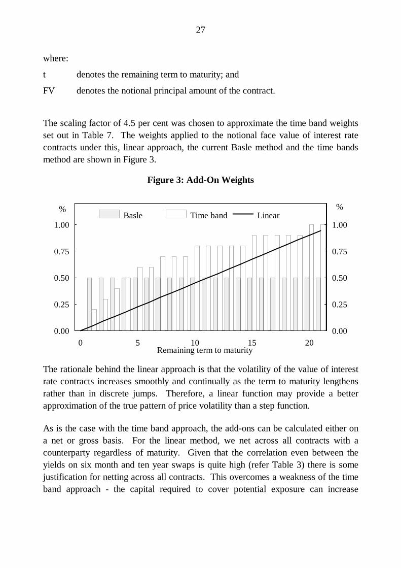
A final approach is one that extends the time bands approach. Rather thanincreasing the weight on notional principal in discrete steps, the potential exposureadd-on is specified as a smooth, linear function of the term to maturity.

That is the add-on can be expressed as:

Add-on = 0.045 x t x FV (5)

15 See Section 5.1.16 Basle Committee on Banking Supervision (1993), Annex 2.

27

where:

t denotes the remaining term to maturity; and

FV denotes the notional principal amount of the contract.

The scaling factor of 4.5 per cent was chosen to approximate the time band weightsset out in Table 7. The weights applied to the notional face value of interest ratecontracts under this, linear approach, the current Basle method and the time bandsmethod are shown in Figure 3.

Figure 3: Add-On Weights

0.00

0.25

0.50

0.75

1.00

0 5 10 15 200.00

0.25

0.50

0.75

1.00Basle Time band Linear

% %

Remaining term to maturity

The rationale behind the linear approach is that the volatility of the value of interestrate contracts increases smoothly and continually as the term to maturity lengthensrather than in discrete jumps. Therefore, a linear function may provide a betterapproximation of the true pattern of price volatility than a step function.

As is the case with the time band approach, the add-ons can be calculated either ona net or gross basis. For the linear method, we net across all contracts with acounterparty regardless of maturity. Given that the correlation even between theyields on six month and ten year swaps is quite high (refer Table 3) there is somejustification for netting across all contracts. This overcomes a weakness of the timeband approach - the capital required to cover potential exposure can increase

28

sharply when closely, but not perfectly, matched contracts fall into separate timebands.

In addition to looking at the gross and net add-ons under the linear approach wecombine the linear approach with the short/long approach. That is the maximumand a weighted average of the add-ons (calculated using equation (5)) on short andlong contracts are also tested in the following sections.

6. RESULTS

6.1 Data

The data used to test the various methods for setting a capital charge consists ofinterest rate swap and forward rate agreement portfolios obtained from a number ofAustralian banks. In some cases the portfolios are complete - covering allcounterparties. In other cases, those counterparties conducting the most businesswith the bank were selected. For the bulk of the portfolios, maximum creditexposure was calculated using the interest rate model and methods detailed inSection 3 and Appendix 1. However, in the case of five portfolios, credit exposurewas calculated by the banks themselves using their own interest rate models andaggregation methods. The number of contracts and counterparties in each portfolioare presented in Table 8.

29

Table 8: Bank Portfolios

Bank Counterparties Contracts

1 214 13022 270 16353 32 2834 43 7735 45 3166 22 937 255 1687Total - RBA model 8818 141 14909 262 162510 54 16411 248 158712 120 --Total - banks' own models 825Total 1706

6.2 Add-Ons

To test the alternative forms of add-ons, each was regressed against maximumpotential exposure. Maximum potential exposure was calculated as the differencebetween maximum credit risk and the current net mark-to-market if positive andzero otherwise. Here, we are testing the ability of the add-on to cover the worstcase increase in a portfolio's value.

For each bank's portfolio, the set of contracts with each counterparty are treated asseparate sub-portfolios. This paper focuses on the structure of the portfolios madeup of the contracts between a bank and one counterparty, rather than the portfolio ofcontracts across all counterparties. Traditionally credit risk analysis has looked at atotal portfolio and argued that since swap portfolios are generally built up so as toavoid any market risk, a swap portfolio can be approximated as a collection ofmatched pairs of the swaps.17 The difficulty with this when addressing the effect ofnetting is that, in most cases the set of contracts with each counterparty are not fullyoffsetting and the extent to which they are offsetting determines the impact ofnetting on both current and potential credit exposure. Hence, the capital charge iscalculated for each counterparty.

17 For example, Board of Governors of the Federal Reserve System and Bank of England (1987).

30

For each bank we regress (across counterparties) the capital charge againstmaximum potential exposure. That is, for each bank and each method of calculatingan add-on, we estimate the equation:

PEi = β Add-oni + εi (6)

where:

PE denotes the estimate of potential exposure obtained using the methods setout in Section 3 and Appendix 1;

Add-on is the capital charge for potential exposure; and

i indexes the bank's counterparties.

The R2 from these regressions are reported in Table 9. Note that the regressions areestimated without the inclusion of a constant, hence it is possible to obtain negativeR2 values. A common problem in cross sectional regression analysis isheteroscedasticity where the variance of the regression errors is not constant. Inmost cases it was found that the error variance increased with the size of thecounterparty portfolio. Hence, the heteroscedasticity was corrected for byperforming weighted least squares estimation using the sum of notional principal foreach counterparty as a scaling factor.

In total, twenty separate methods were tested as a capital charge for potentialexposure. They fall into seven broad groups.

1. The standard Basle add-on together with two different ways of calculating netmark-to-market. The first alternative calculates the net mark-to-market (NetRC) as the sum of the market value of all contracts in the portfolio if this sumis positive, and zero otherwise. This is the conventional way of calculating netcredit exposure. It can be seen that except for one bank the net replacementcost performs poorly compared to the Basle approach. The second 'net'calculation (ABS Net) is to take the absolute value of the sum of the marketvalue of the portfolio's contracts. This provides a much better measure ofpotential exposure, outperforming the conventional net measure in every case.It is more highly correlated with potential exposure than the Basle measure in anumber of cases, but overall fails to out-perform the Basle add-ons.

31

2. The second group of capital charges are those suggested by ISDA and aredenoted in Table 9 as ISDAC1, ISDAC2 and ISDAC3. They are calculatedfrom equations (3) and (4), using the conventional definition of net (the sum ofthe contracts' market values if positive and zero otherwise) and gross (the sumof the positive market values in a portfolio). ISDAC1 is calculated fromequation (3). ISDAC2 is calculated using equation (4) with β set equal to 0.25(the value suggested by ISDA as being appropriate). A grid search was usedto find an optimal value of β at 0.35. ISDAC3 is calculated using that value ofβ. For all banks, ISDAC2 and ISDAC3 are more highly correlated withpotential exposure than ISDAC1.

3. The third group of measures, comprising ISDA1 and ISDA2, are alsocalculated from equations (3) and (4), but are based on the absolute net-to-gross ratio (that is, the absolute value of the sum of all contracts' net marketvalue divided by the sum of the absolute market value of each contract). In thiscase, a grid search confirmed 0.25 as the appropriate value for β. Thesemeasures strongly out-rank those using the conventional net ratio in all casesexcept one. Because very few counterparties have a net market value of zerothere is little difference in the explanatory power of the two formulations(ISDA2 outranking ISDA1 in five of the nine banks).

32

Table 9: Correlation Between Maximum Potential Exposure and the Proposed Add-Ons (R2)

Bank 1a Bank 2 Bank 3a Bank 4a Bank 5a Bank 6 Bank 7a All - Fed modela Bank 8 Bank 9a Bank 10a Bank 11

Basle 0.0731 0.0540 0.3392 0.0087 0.1295 0.2142 0.3862 0.2165 0.1340 0.3087 0.1066 0.2830Net RC -0.3302 -0.2705 0.0590 0.1321 -1.1168 -0.2409 -0.2198 -0.4928 -0.2097 0.1535 -0.6911 0.0578ABS Net -0.1847 0.3556 0.4425 0.6087 -0.0226 0.0118 0.3086 -0.2524 0.2646 0.4033 -0.0658 0.4187

ISDAC1 -0.3615 -0.0770 0.0428 0.0805 -0.2305 0.0001 0.1999 -0.0835 -0.0148 -- -0.4616 -0.7735ISDAC2 -0.1735 -0.0156 0.2602 0.1489 0.0030 0.0714 0.3127 0.0636 0.1257 -- -0.1934 0.3587ISDAC3 -0.1132 0.0022 0.3050 0.1414 0.0546 0.0965 0.3406 0.1054 0.1455 -- -0.1152 0.3587

ISDA1 0.2871 0.1647 0.7340 0.3526 0.2276 0.2345 0.4829 0.3589 -0.0090 -- 0.1321 --ISDA2 0.2754 0.1505 0.6862 0.3141 0.3002 0.2387 0.4949 0.3573 0.1299 -- 0.2034 --

Short/Long:Maximum 0.1923 0.1320 0.5651 0.0599 0.2497 0.2382 0.5092 0.3309 0.0773 0.3246 0.1789 0.4169Net 0.2488 0.2015 0.5825 -0.0841 0.1617 0.1906 0.5328 0.3601 0.0062 0.2730 0.0460 0.5972Weighted 0.2502 0.1953 0.6223 -0.0213 0.2126 0.2066 0.5455 0.3701 0.0196 0.2894 0.0977 0.5760

+/- MTM:Maximum 0.1989 0.1318 0.5631 0.0559 0.2109 0.2382 0.4840 0.3202 0.1082 -- 0.1789 0.4371Net 0.2765 0.2027 0.5825 -0.0793 0.0780 0.1906 0.4733 0.3385 -0.0078 -- 0.0460 0.5593Weighted 0.2632 0.1850 0.6385 0.0185 0.1754 0.2193 0.5031 0.3537 0.0445 -- 0.1360 0.5603

Time band:Gross 0.2503 0.1825 0.5416 0.2831 0.3994 0.2139 0.3836 0.3535 0.1220 0.3138 0.1909 0.2639Net 0.4313 0.3331 -0.1443 0.5652 0.1912 0.3154 0.4315 0.4173 0.0700 0.2796 0.0620 --

Linear:Gross 0.2865 0.1802 0.5193 0.3089 0.4126 0.1580 0.3665 0.3562 0.1539 0.2842 0.1707 --Maximum 0.4185 0.3116 0.7743 0.4954 0.4827 0.2545 0.4701 0.4807 0.0874 0.2759 0.2748 --Net 0.4824 0.4590 0.8978 0.5210 0.3882 0.2227 0.4917 0.5241 0.0156 0.2170 0.0291 --Weighted 0.4802 0.4326 0.9114 0.5677 0.4334 0.2501 0.3020 0.5299 0.0322 0.2361 0.1402 --

Note: a Estimation by weighted least squares.

33

Table 10: Correlation Between Total Credit Exposure and the Proposed Capital Charges (R2)

Bank 1a Bank 2a Bank 3a Bank 4a Bank 5a Bank 6 Bank 7a All - Fed modela Bank 8 Bank 9a Bank 10 Bank 11 Bank 12

Basle 0.9954 0.7498 0.7186 0.2201 0.6264 0.9882 0.8016 0.9779 0.6706 0.6109 0.8644 0.9903 0.9998Basle alternative 0.9951 0.7248 0.6290 0.0884 0.5833 0.9862 0.7682 0.9757 0.6368 0.5964 0.8511 0.9887 --

Scenario 0.9956 0.7425 0.6329 0.1910 0.6196 0.9889 0.7827 0.9791 -- -- 0.8884 -- --

ABS Net 0.9959 0.8479 0.8504 0.3069 0.6501 0.9873 0.8403 0.9810 0.5456 0.5989 0.8111 0.9736 0.9991

ISDA1 0.9953 0.7471 0.6987 0.1253 0.5941 0.9881 0.7873 0.9768 0.5637 -- 0.8378 -- 0.9998ISDA2 0.9953 0.7479 0.7044 0.1518 0.6027 0.9881 0.7911 0.9771 0.6193 -- 0.8449 -- 0.9998

Short/Long:Maximum 0.9954 0.7492 0.7062 0.1812 0.6138 0.9881 0.7960 0.9775 0.6554 0.6079 0.8583 0.9896 0.9260Net 0.9953 0.7483 0.6912 0.1347 0.6000 0.9879 0.7898 0.9770 0.6329 0.6045 0.8507 0.9881 0.3690Weighted 0.9960 0.7818 0.7786 0.2728 0.6560 0.9898 0.8283 0.9806 0.4884 0.6192 0.8819 0.9874 --

Time band:Gross 0.9953 0.7492 0.6925 0.1891 0.6181 0.9872 0.7690 0.9772 0.6742 0.6074 0.8598 0.9896 0.9998Net 0.9952 0.7492 0.6522 0.1656 0.5964 0.9873 0.7843 0.9766 0.6557 0.6055 0.8597 -- 0.9998

Linear:Gross 0.9880 0.8481 0.3880 0.4401 0.8042 0.9593 0.8162 0.8974 0.1091 0.4402 0.5300 -- --Maximum 0.9935 0.9116 0.5884 0.6702 0.9215 0.9893 0.8904 0.9391 0.0643 0.5053 0.6463 -- --Net 0.9961 0.9251 0.7484 0.7019 0.9389 0.9892 0.8892 0.9606 0.0145 0.5362 0.6115 -- --Weighted 0.9485 0.8279 0.3700 0.5676 0.8891 0.9778 0.7581 0.7392 0.0019 0.4140 0.4346 -- --

Note: a Estimation by weighted least squares.

34

4. The fourth set of add-ons measure the capital charge as a function of short andlong positions. First, the maximum of the sum of the Basle add-ons on all shortand long contracts was taken. Second, the absolute difference between thetotal add-ons on short and long contracts was considered (this is denotedshort/long net in the table). Finally, a weighted sum of the Basle add-ons (thatis, the short/long gross add-on) and the short/long net position is calculated.The respective weights were determined by regressing the two components ofthe weighted sum against maximum potential exposure. The optimal weightsestimated were 23 per cent of the net add-ons and 2 per cent of gross add-ons.This reflects a strong correlation between the swap rates in the portfolios.Moving from the net short/long to the weighted short/long adds little to theexplanatory power of the capital charge. The net add-ons tend to performbetter than the maximum of the short and long add-ons.

5. The fifth group of add-ons approximate the short/long approach by splitting theportfolio between positively and negatively valued contracts. On the whole,these measures performed much like the short/long add-ons. The short/longapproach appears to be slightly better at tracking potential exposure. Thepositive/negative approach can be expected to be a reasonably good proxy forthe short/long add-ons given that swap rates have steadily declined for the fouryears prior to the date these portfolios were selected and that the averageremaining term to maturity of the contracts is quite short (three-quarters of thecontracts have a remaining term to maturity of less than three years). Furtherdetails of the maturity profile of the portfolios is presented in Table 11. Oncethe interest cycle moves beyond a turning point the performance of this set ofadd-ons can be expected to deteriorate. Moreover, while the interest rate cycleis fairly smooth, other asset prices such as foreign exchange rates tend not tofollow such smooth cycles and so this approach may not be appropriate forforeign exchange and derivatives written against other commodities.

6. The sixth group are those based on the time band approach, the first beingbased on the gross time band, the second, on net time bands. In all cases,except one, the gross time band out-performs the Basle add-ons. Overall, thenet time bands outperform the gross time band add-ons. However, the netadd-ons perform poorly for several banks.

35

Table 11: Maturity Breakdown(percentage of portfolio in each maturity band)

Years: <1 1-2 2-3 3-4 4-5 5-7 7-10 10-15 15-20

Bank1 42.78 30.26 15.90 6.53 2.76 1.38 0.38 0.00 0.002 45.44 23.73 11.80 7.40 4.04 4.95 2.51 0.06 0.063 30.39 26.50 21.91 12.72 4.24 2.83 1.41 0.00 0.004 39.97 24.45 17.46 7.24 2.85 4.27 3.75 0.00 0.005 22.78 24.05 14.87 11.08 7.59 10.44 8.86 0.32 0.006 29.03 45.16 15.05 5.38 4.30 0.00 1.08 0.00 0.007 29.16 26.08 18.44 7.71 5.99 8.42 4.03 0.18 0.008 35.17 24.70 16.11 7.79 5.70 6.31 3.76 0.47 0.009 45.17 23.88 11.88 7.38 4.06 4.98 2.52 0.06 0.0610 12.20 17.07 29.27 12.80 9.15 10.98 8.54 0.00 0.0011 -- -- -- -- -- -- -- -- --12 -- -- -- -- -- -- -- -- --

7. The final group of add-ons are based on the linear function, equation (5). Thegross measure (simply summing the add-ons for each contract) outperformsBasle and is on par with the detailed time bands gross result. The net measure,which nets the add-ons across all contracts for each counterparty doesparticularly well - overall outperforming the net time bands method. Aweighted sum of the gross linear add-ons and the net linear add-ons, withweights of 3 per cent and 22 per cent respectively, improved slightly on the netadd-on.

The results presented in Table 9 suggest that the Basle method outperforms theother measures in group 1 and those in group 2, but is itself outperformed, overall,by the measures shown under groups 3, 4, 5, 6 and 7. The one approach whichappears to correlate most closely with potential exposure is the weighted linear add-on. The net linear add-on also performs particularly well.

These overall results hold, broadly speaking, for individual bank portfolios. Therewere, however, exceptions. The weighted linear add-on, the best overall measure,performed very poorly in the case of one bank (bank 10). In contrast, despite the

36

inability of the ABS Net measure to track potential exposure across all banks, itgenerated relatively good results in the case of some individual banks (banks 4, 8and 9).

6.3 Total Capital Charge

To test whether a total capital charge should be based on equation (1) (Baslepreferred method) or equation (2), both measures were calculated using the Basleadd-ons and were regressed against the modelled total credit exposure. For eachbank and each method of setting a total capital charge, we estimate the equation

TEi = β Chargei + εi (7)

where:

TE denotes the estimate of total credit exposure obtained using the methods setout in Section 3 and Appendix 1;

Add-on is the total capital charge; and

i indexes the bank's counterparties.

The R2 from these regressions are reported in Table 10. From Table 10 it can beseen that while the two approaches have practically the same explanatory power,the current Basle approach consistently outperformed the alternative. Thiscomparison was performed using different methods of calculating the add-on, withthe same result. This seems to be due to the fact that the add-ons tend tounderestimate the increase in exposure and the standard, more conservative,approach to the calculation of the capital charge compensates for this.

The scenario approach, looking at the worst case credit exposure from current rates,and from up and down shifts in the yield curve, provides similar explanatory poweras the Basle approach.

In the light of the results of the add-on tests, the following add-ons were included ina test of the total capital charge:18

18 The current exposure and the add-on were combined using the method proposed by Basle, that

is using equation (4).

37

• the absolute value of net mark-to-market;

• the absolute net-to-gross ratios;

• the time band approach;

• the short/long approach; and

• the linear approach.

The results show that the variation in total exposure across counterparty portfolios isso dominated by current exposure that there is little to distinguish between thedifferent add-on approaches. Overall, none of the formulations dominate the currentBasle proposal by any significant margin.

These results are based on a comparison of the capital measures with the maximumpotential exposure and maximum total exposure. In other words, capital is held tocover the possibility of counterparty failure at the worst possible time. A lessstringent assumption is that a counterparty fails on any given day during the life ofits contracts. In this case, it is more appropriate to consider the capital coverage interms of average potential exposure and average total exposure. The results usingthese assumptions are presented in Appendix 2. The conclusions reached from thisare broadly consistent with the results obtained from the analysis of maximumexposure. However, the relative performance of the net linear method improvessomewhat.

6.4 Offsetting Contracts

The above results were obtained using static portfolios. One possibility is that therecognition of netting within the capital standards may provide an incentive forbanks to enter into a greater number of offsetting contracts.

To test the effect of banks taking on a higher proportion of offsetting business, onlythose counterparties with two-way deals with banks 1 to 7 were selected and thecapital charges were tested on this sub-sample. The results of this are presented inTable 12. Again, when considering the add-ons alone, the ISDA, the time band, theshort/long and the linear approaches outperform the current Basle add-ons. The netand weighted linear methods are most strongly correlated with potential exposure.In the test of the total capital charge, however, there is no great difference in

38

explanatory power between any of the proposed methods (the Basle methodincluded).

Table 12: Counterparties with Two-Way Contracts: R2 from Regressing theCapital Charge Against Modelled Exposurea

Add-ons Total capital charge

Basle 0.1977 Basle 0.9900Net RC -0.5415 Basle alternative 0.9887ABS Net -0.2998

Scenario 0.9906ISDAC1 0.2705ISDAC2 0.2977 ABS Net 0.9906ISDAC3 0.2927

ISDA1 0.9889ISDA1 0.2705 ISDA2 0.9892ISDA2 0.2977

Short/Long:Short/Long: Maximum 0.9895Maximum 0.2873 Net 0.9890Net 0.2709 Weighted 0.9909Weighted 0.2964

+/- MTM:+/- MTM: Maximum 0.9895Maximum 0.2650 Net 0.9889Net 0.2208 Weighted 0.9909Weighted 0.2686

Time band:Time band: Gross 0.9894Gross 0.2846 Net 0.9889Net 0.2896

Linear:Linear: Gross 0.9020Gross 0.2824 Maximum 0.9485Maximum 0.3792 Net 0.9734Net 0.3826 Weighted 0.8009Weighted 0.4042

Notes: a Estimation by weighted least squares.

39

6.5 A Different Yield Curve

All the preceding results obtained took the beginning of 1994 as the starting pointfor the interest rate simulations. This was, in all likelihood, close to the trough inthe Australian interest rate cycle. To test the sensitivity of the results to the level ofinterest rates the credit risk calculations were performed a second time using rates atthe beginning of 1992 (initial short rate 7.4 per cent and long rate 9.75 per cent) forone actual portfolio and one randomly generated portfolio.19 The results, for boththe 1994 and 1992 credit risk calculations are shown in Tables 13 and 14.

Table 13: Shifts in the Yield Curve: Correlation Between Maximum PotentialExposure and the Proposed Add-Ons (R2)

Actual 1994 Actual 1992 Random 1994 Random 1992

Basle 0.2760 0.2519 0.0072 0.0171Net RC -0.3526 -0.5376 -0.0854 -0.9098ABS Net 0.1562 -0.0356 0.2891 0.0199

ISDAC1 -0.1547 -0.7556 -0.7298 -1.2703ISDAC6a 0.2057 -0.1583 -0.2208 -0.4000

Short/Long:Maximum 0.3272 0.3686 0.0885 0.1258Net 0.2011 0.3391 -- --Weighted 0.2496 0.3706 -- --

Net time band 0.1606 0.4006 0.0833 0.1469

Linear:Gross 0.2955 0.4178 -- --Maximum 0.3780 0.5226 -- --Net 0.1959 0.3285 -- --Weighted 0.2865 0.4293 -- --

Note: a ISDAC6 is the conventional ISDA formulation calculated with b set equal to 0.6.

19 The size of the randomly generated portfolio was doubled by creating an exactly offsetting deal

for each initial deal. Hence the net market value of the total portfolio is zero.

40

Table 14: Shifts in the Yield Curve: Correlation between Total CreditExposure and the Proposed Total Capital Charge (R2)

Actual 1994 Actual 1992 Random 1994 Random 1992

Basle 0.8644 0.3202 0.9693 0.5185Basle alternative 0.8511 0.2371 0.9564 0.4106Scenario 0.8884 0.6000 0.9623 0.6099

ABS Net 0.8111 0.2373 0.9341 0.4925

ISDAC1 0.8377 0.1772 0.9532 0.3727ISDAC6a 0.8534 0.2636 0.9638 0.4619

Short/Long:Maximum 0.8583 0.3086 0.9653 0.4844Net 0.8507 0.2923 -- --Weighted 0.8819 0.4286 -- --

Net time band 0.8597 0.2590 0.9605 0.436

Linear:Gross 0.5300 0.4982 -- --Maximum 0.6463 0.6337 -- --Net 0.6115 0.5565 -- --Weighted 0.4346 0.5043 -- --

Note: a ISDAC6 is the conventional ISDA formulation calculated with β set equal to 0.6.

Turning first to the comparison of the add-ons with potential exposure, when the1992 interest rate scenario is adopted, the performance of the net time band, theshort/long and the linear add-ons improves. In the case of the total capital charge,however, the explanatory power of all formulations falls significantly, except thelinear approach. The linear and scenario approaches appear to be most robust to theshift in the yield curve, however the scenario approach clearly outranks the linearapproach under the 1994 interest rate scenarios.

This result introduces a note of caution in interpreting the results and in imposing acapital charge; the level of interest rates can have an effect on outcomes.

41

7. COVERAGE

This section presents some evidence on the extent to which credit exposure fallswhen moving from a non-netting to a netting environment.

The reduction in replacement cost (current exposure) depends upon the compositionof each bank's portfolio; in particular the value of out-of-the-money contracts. Forbanks 1 to 7, we estimate that moving from calculating current exposure on a grossbasis to a net basis, will reduce replacement cost by an average of 33 per cent (seeTable 15). This assumes that netting agreements are concluded with allcounterparties who conduct two-way business.

It is quite possible that, in a netting environment, the reduction in current exposuremay be larger (both in proportional and absolute terms) than the reduction inmaximum future exposure, which implies that potential exposure may in factincrease. Consider the case of a portfolio of contracts with negative market valueoverall, but which contains some positively valued contracts. The gross currentcredit exposure will have some positive value, while the net current exposure will bezero. Hence, adoption of netting will result in a 100 per cent reduction in currentcredit exposure. However, it is quite possible that in both the gross and netenvironments, future potential exposure will take on some positive value. While thegross potential exposure may be considerably higher than the net potential exposure,so long as net potential exposure is positive, the proportionate reduction in potentialexposure when moving from gross to net will be less than 100 per cent.

Table 15 shows that the average increase in the gap between maximum exposureand the capital held for current exposure is small, at just one per cent. However, forindividual banks the gap can increase by as much as 30 per cent. Reflecting this,Table 16 shows that the coverage of potential exposure by the Basle add-on is littledifferent, overall, between the netted and non-netted scenarios. Table 16 alsodemonstrates that while the Basle measure of credit exposure covers only aproportion of maximum credit exposure (a reflection, in part of the comparativelysevere assumptions behind this measure of exposure) it more than adequately coversaverage credit exposure.

42

Table 15: Percentage Change from Non-Netted to Netted Exposure

The gap between totalexposure and current

exposure:

Maximumexposure

Averageexposure

Capital forcurrent exposure

Maximumexposure

Averageexposure

Bank 1 -16.89 -39.42 -20.88 -6.53 2.15Bank 2 -18.66 -21.44 -25.13 -7.08 -31.89Bank 3 -36.11 -32.46 -14.61 -41.46 -49.10Bank 4 -35.12 -39.72 -70.04 31.17 -123.89Bank 5 -13.77 -19.49 -43.92 27.75 -200.28Bank 6 -8.34 -9.13 -7.78 -10.21 -6.45Bank 7 -21.55 -23.69 -37.59 8.77 -70.99

Total -20.98 -27.53 -33.13 1.02 -44.59

Table 16: Coverage

Percentage of potentialexposure covered by the

Basle add-ons

Percentage of total exposurecovered by the Basle

credit equivalent

Non-netted Netted Non-netted Netted

Maxexposure

Avgexposure

Maxexposure

Avgexposure

Maxexposure

Avgexposure

Maxexposure

Avgexposure

Bank 1 10.99 100.00 11.76 100.00 76.27 190.63 72.45 248.41Bank 2 10.98 100.00 11.82 100.00 65.39 157.44 63.92 159.33Bank 3 7.78 29.18 13.28 57.34 33.36 80.89 36.35 83.36Bank 4 18.17 100.00 13.85 111.18 68.73 163.99 39.91 102.49Bank 5 10.83 100.00 8.48 58.04 59.54 118.84 42.96 91.83Bank 6 20.78 100.00 23.14 100.00 145.02 380.73 82.69 219.00Bank 7 12.60 100.00 11.59 100.00 65.40 141.59 57.59 128.18

Total 11.98 100.00 11.86 100.00 64.43 148.81 59.93 150.90

43

8. CONCLUSION

There are strong theoretical arguments in favour of a more sophisticated approach tosetting a credit risk capital charge when obligations are netted. However, empiricalsupport for these arguments does not appear to be as strong. The work withAustralian banks' portfolios provides some evidence to suggest that a number ofapproaches to the calculation of the add-on provides a more efficient coverage ofpotential exposure than the current Basle formula, namely:

• the current Basle add-on scaled by the absolute ratio of net to gross market value;

• the short/long approach;

• a method which allows the add-ons for contracts within given time bands to benetted; and

• a smooth, rather than stepped, function of term to maturity.

The approach to the calculation of a total capital charge which appears most robustto interest rate movements over the cycle is the scenario approach. While severalapproaches are some improvement over the proposed method, no single formulationclearly outranks all others.

The better performance of these alternative approaches to capturing potentialexposure is not sufficient to outweigh the dominance of current exposure in thedetermination of the total capital charge. So long as the coverage of potentialexposure afforded by the add-ons remains low relative to that provided for currentexposure, and that is one conclusion of this work, then the capital charge willcontinue to be dominated by current exposure. That suggests that the case for amore complex formulation of the capital charge is not warranted.

The conclusions of the analysis are, nonetheless, tentative since the work coversonly portfolios comprising simple interest rate swaps and forward rate agreements.Exchange rate and other, more complex, derivatives have not been considered. Theadd-on factors for exchange rate contracts are considerably higher than those forinterest rate contracts. Hence, the add-ons for a portfolio made up of both interestrate and other contracts could represent a higher proportion of the total capitalcharge than for a portfolio of interest rate contracts alone. This remains anempirical question since current exposure on these contracts could also be higher.Whether the add-ons represent a higher or lower proportion of the total capitalcharge for more complex portfolios, will depend upon the composition of theportfolio and on market conditions.

44

APPENDIX 1

A1.1 Interest Rate Model

The model used to generate the time paths for interest rates is that used by theFederal Reserve Bank of New York (FRBNY) in some of its work on netting. Thismodel incorporates a simple curved and varying term structure.20 The two endpoints of the yield curve are allowed to vary stochastically over time and all pointsbetween these two are determined by an exponentially weighted average of thosetwo yields.

Movements in the short yield are assumed to be driven by two factors. Firstly, theshort yield is taken to drift towards the current long yield at a fixed speeddetermined by the parameter k. Secondly, a random shock, ε , is added to thisprocess. The standard deviation of this shock is taken to be proportional to theshort yield. The discrete approximation to this process is:

St+1 = St + k (Lt - St) ∆t + ε St ∆t (A1)

where:

t denotes time;

St is a short yield;

Lt is a long yield;

ε is a standard normal deviate; and

k is the rate of reversion of the short rate towards the long rate.

The long yield is modelled as geometric Brownian motion with no drift.

dL = σ L dz (A2)

where:

dz is a Wiener process.

20 The FRBNY has conducted work using this model and the more sophisticated model

developed by Longstaff and Schwartz (1992). While the simpler model we use lacks thetheoretical rigour of the latter model the FRBNY found that, for their work, the two modelsyielded similar results.

45

Hence the logarithm of the long rate can be taken to be distributed normally:

Mt ~ N(M0 - σ2t/2,σ2t) (A3)

where:

Mt = ln(Lt); and

M0 is the current value of M.

While the long rate is characterised as geometric Brownian motion with no drift,there is drift in the process determining the log of the long rate, Mt. This drift term,-σ2t, is reflected in the simulation process to prevent the simulated interest ratepaths from drifting upwards. The stochastic processes ε and dz are assumed to beindependent.

Given a short and long yield, yields for any maturity are derived using the followingequation:

y(τ) = L + (S - L) (1 - e-kτ)

kτ (A4)

where:

y(τ) denotes the yield for maturity to τ.21

Parameters for this model were obtained using weekly observations of the 90-daybank bill rate and the ten-year government bond rate over the period January 1984to August 1993. σ was estimated to be equal to 0.1, and k was estimated at 0.46.

21 Note that the model's long rate is in fact the rate on a security with infinite term to maturity,

that is, y(t) = Lt only when t → ∞ . Equation (3) can be modified so that y(10) = Lt by

replacing Lt with L*t where L*

t = Lt - fSt1 - f and f = (1 - e -10k)/10k. That is equation (3) is

rewritten as y(τ) = L* + (S - L*) (1 - e-kτ)

kτ . For our simulations we do not employ this

adjustment, but simply use equation (3) above.

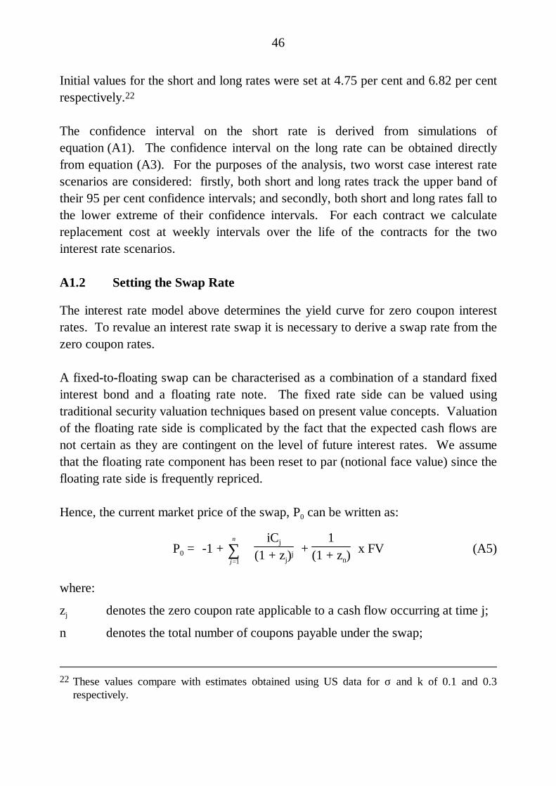
46

Initial values for the short and long rates were set at 4.75 per cent and 6.82 per centrespectively.22

The confidence interval on the short rate is derived from simulations ofequation (A1). The confidence interval on the long rate can be obtained directlyfrom equation (A3). For the purposes of the analysis, two worst case interest ratescenarios are considered: firstly, both short and long rates track the upper band oftheir 95 per cent confidence intervals; and secondly, both short and long rates fall tothe lower extreme of their confidence intervals. For each contract we calculatereplacement cost at weekly intervals over the life of the contracts for the twointerest rate scenarios.

A1.2 Setting the Swap Rate

The interest rate model above determines the yield curve for zero coupon interestrates. To revalue an interest rate swap it is necessary to derive a swap rate from thezero coupon rates.

A fixed-to-floating swap can be characterised as a combination of a standard fixedinterest bond and a floating rate note. The fixed rate side can be valued usingtraditional security valuation techniques based on present value concepts. Valuationof the floating rate side is complicated by the fact that the expected cash flows arenot certain as they are contingent on the level of future interest rates. We assumethat the floating rate component has been reset to par (notional face value) since thefloating rate side is frequently repriced.

Hence, the current market price of the swap, P0 can be written as:

P0 =

-1 +

j

n

=∑

1

iCj

(1 + zj)j + 1

(1 + zn) x FV (A5)

where:

zj denotes the zero coupon rate applicable to a cash flow occurring at time j;

n denotes the total number of coupons payable under the swap;

22 These values compare with estimates obtained using US data for σ and k of 0.1 and 0.3

respectively.

47

Cj is equal to the jth coupon period;

FV is the notional principal amount; and

i is the swap rate.23

To determine the swap rate, i, we assume that at the date the swap is written theswap rate is set such that the current market price of the swap is zero. That is,equation (A5) is solved for i setting P0 equal to zero. In theory competitive forceswithin the swap market should ensure that this condition holds.

For example, consider a 3-year swap, written on 20 September 1992 with fixed ratepayments payable semi-annually, and the following zero coupon rates substitutingthese values into equation (A5) and setting P0 equal to zero yields a swap rate of5.57 per cent.

Table A1: Zero Coupon Rates

Coupon dates Zero couponyield curve

zj

Coupon period(years)

Cj

20 Mar 92 4.96 0.498620 Sep 92 5.15 0.504120 Mar 93 5.30 0.495920 Sep 93 5.44 0.504120 Mar 94 5.56 0.495920 Sep 94 5.67 0.5041

To summarise the process for an individual contract: at each point in time, a worstcase zero coupon yield curve is observed. From that yield curve, a swap revaluationrate is calculated which is the market rate to replace the remaining cash flows of theswap. The present value of the difference between the swap's cash flows and thepayments made under the replacement swap is calculated to give the value at risk ifthe counterparty were to default. These steps are repeated at weekly intervals overthe life of the swap to generate a time path for the credit exposure of the contract.

23 This is an extension of the formula given in Das (1994) p. 192.

48

APPENDIX 2

Table A2: Correlation Between Average Potential Exposure and the ProposedAdd-Ons (R2)

Bank 1a Bank 2 Bank 3a Bank 4 Bank 5a Bank 6 Bank 7a All - Fedmodela

Basle -0.0314 -0.0788 0.3254 0.0709 0.0140 -0.2392 0.2410 0.1879Net RC -0.3519 0.0836 0.3375 0.5025 -0.2380 -0.2736 0.2065 -0.0110ABS Net -0.3517 0.0938 0.3401 0.6314 -0.0872 -0.2722 0.2202 -0.0071

ISDAC1 -0.3393 -0.1362 0.0512 0.2778 -0.3089 -0.2749 0.1325 0.2112ISDAC2 -0.2513 -0.1207 0.2392 0.2367 -0.1675 -0.2687 0.1950 0.2240ISDAC3 -0.2112 -0.1140 0.2798 0.2072 -0.1248 -0.2656 0.2109 0.2219

ISDA1 0.1308 -0.0418 0.6933 0.3615 -0.0151 -0.2420 0.3457 0.3293ISDA2 0.1059 -0.0500 0.6400 0.2836 0.0389 -0.2410 0.3352 0.2960

Short/Long:Maximum 0.0619 -0.0564 0.5263 0.1286 0.0332 -0.2358 0.3262 0.2822Net 0.1390 -0.0283 0.5634 0.1013 -0.0514 -0.2339 0.3680 0.3930Weighted 0.1308 -0.0333 0.5924 0.1346 -0.0215 -0.2341 0.3694 0.3823

+/- MTM:Maximum 0.0700 -0.0562 0.5263 0.1382 0.0129 -0.2358 0.3166 0.1825Net 0.1670 -0.0273 0.5634 0.1440 -0.0947 -0.2339 0.3460 0.2158Weighted 0.1381 -0.0371 0.6014 0.1717 -0.035 0.2343 0.3487 0.2152

Time band:Gross 0.1228 -0.0203 0.5157 0.1884 0.1335 -0.235 0.2263 0.1937Net 0.2638 0.0527 -0.0974 0.4199 0.0017 -0.2111 0.2711 0.2370

Linear:Gross 0.1604 -0.0133 0.481 0.1991 0.1358 -0.2385 0.2147 0.2054Maximum 0.2805 0.0454 0.7157 0.3199 0.1509 -0.2408 0.2855 0.2941Net 0.3744 0.1332 0.8587 0.3923 0.0918 -0.2484 0.3219 0.3458Weighted 0.3599 0.1127 0.8598 0.4216 0.1154 -0.2461 0.3211 0.3425

Notes: a Estimation by weighted least squares.

49

Table A3: Correlation Between Average Total Credit Exposure and theProposed Total Capital Charge (R2)

Bank 1a Bank 2a Bank 3a Bank 4a Bank 5a Bank 6a Bank 7a All - Fedmodela

Basle 0.9665 0.6054 0.8844 0.5155 0.5649 0.4979 0.7658 0.7304Baslealternative

0.9659 0.5874 0.8524 0.4785 0.5337 0.4799 0.7437 0.7244

Scenario 0.9681 0.6250 0.8415 0.5338 0.5681 0.5341 0.7673 0.7568

ABS Net 0.9671 0.6599 0.8982 0.4094 0.5687 0.4837 0.7785 0.7195

ISDA1 0.9662 0.6063 0.8813 0.4896 0.5413 0.4972 0.7564 0.7188ISDA2 0.9663 0.6062 0.8827 0.4979 0.5476 0.4974 0.7589 0.7218

Short/Long:Maximum 0.9663 0.6072 0.8833 0.5121 0.5561 0.4974 0.7629 0.7239Net 0.9662 0.6087 0.8798 0.5040 0.5463 0.4967 0.7594 0.7171Weighted 0.9678 0.6312 0.9091 0.5484 0.5909 0.5202 0.7895 0.7343

+/- MTM:Maximum 0.9663 0.6073 0.8833 0.5118 0.5544 0.4974 0.7618 0.7848Net 0.9662 0.6088 0.8798 0.5038 0.5429 0.4967 0.7572 0.7836Weighted 0.9677 0.6294 0.9085 0.5466 0.5858 0.5193 0.7853 0.7934

Time band:Gross 0.9662 0.6096 0.8771 0.5183 0.5613 0.4909 0.7580 0.7246Net 0.9661 0.6114 0.8615 0.5133 0.546 0.4923 0.7546 0.7169

Linear:Gross 0.9844 0.6529 0.2110 0.2087 0.6694 0.6128 0.6981 0.8910Maximum 0.9886 0.7340 0.3401 0.3617 0.7969 0.6848 0.7936 0.9184Net 0.9899 0.7815 0.4683 0.4665 0.8442 0.7025 0.8282 0.9224Weighted 0.9743 0.6957 0.1362 0.2927 0.7877 0.7258 0.6838 0.8499

Notes: a Estimation by weighted least squares.

50

REFERENCES

Bank for International Settlements (1990), Report of the Committee on InterbankNetting Schemes of the Central Banks of the Group of Ten Countries (also knownas the Lamfalussy Report), Basle, November.

Basle Committee on Banking Supervision (1993), The Supervisory Treatment ofMarket Risks, Basle, April.

Board of Governors of the Federal Reserve System and Bank of England(1987), 'Potential Credit Exposure on Interest Rate and Foreign Exchange RateRelated Instruments', unpublished technical paper.

Das, S. (1994), Swaps and Financial Derivatives, IFR Publishing Ltd, London.

Estrella, A. (1992), 'Gross Notional Principal, Net Replacement Cost, and thePotential Credit Exposure of Plain Vanilla Swaps', Federal Reserve Bank ofNew York, unpublished technical working paper.

Estrella, A. (1993), 'Netting and Potential Exposure: A Simple StatisticalIllustration', Federal Reserve Bank of New York, unpublished technical workingpaper.

Estrella, A. and D. Hendricks (1993), 'Netting and Potential Exposure: A SimpleStatistical Illustration', Federal Reserve Bank of New York, unpublished technicalworking paper.

Frye, J. (1992), 'Underexposed and Overanxious', Risk, 5(3), pp. 41-47.

Hendricks, D. (1992), 'Swap Credit Exposure Add-ons: Portfolio and NettingEffects', Federal Reserve Bank of New York, unpublished technical working paper.

Gumerlock, R. (1993), 'Double Trouble', Risk, 6(9), pp. 80-91.

Levonian, M. (1994), 'Bank Capital Standards for Foreign Exchange and OtherMarket Risks', Federal Reserve Bank of San Francisco, Economic Review, March,pp. 3-18.

51

Longstaff, F. and E. Schwartz (1992), 'Interest Rate Volatility and the TermStructure: A Two-Factor General Equilibrium Model', The Journal of Finance,47(4), pp. 1259-1282.

Reserve Bank of Australia (1990), Prudential Supervision of Banks, ReserveBank of Australia, Sydney.

Simons, K. (1993), 'Interest Rate Structure and the Credit Risk of Swaps', NewEngland Economic Review, July/August, pp. 23-34.