deep neural networks rival the representation of...

Deep Neural Networks Rival the Representation ofPrimate IT Cortex for Core Visual Object RecognitionCharles F. Cadieu1*, Ha Hong1,2, Daniel L. K. Yamins1, Nicolas Pinto1, Diego Ardila1, Ethan A. Solomon1,

Najib J. Majaj1, James J. DiCarlo1

1 Department of Brain and Cognitive Sciences and McGovern Institute for Brain Research, Massachusetts Institute of Technology, Cambridge, Massachusetts, United States

of America, 2 Harvard–MIT Division of Health Sciences and Technology, Institute for Medical Engineering and Science, Massachusetts Institute of Technology, Cambridge,

Massachusetts, United States of America

Abstract

The primate visual system achieves remarkable visual object recognition performance even in brief presentations, andunder changes to object exemplar, geometric transformations, and background variation (a.k.a. core visual objectrecognition). This remarkable performance is mediated by the representation formed in inferior temporal (IT) cortex. Inparallel, recent advances in machine learning have led to ever higher performing models of object recognition usingartificial deep neural networks (DNNs). It remains unclear, however, whether the representational performance of DNNsrivals that of the brain. To accurately produce such a comparison, a major difficulty has been a unifying metric that accountsfor experimental limitations, such as the amount of noise, the number of neural recording sites, and the number of trials,and computational limitations, such as the complexity of the decoding classifier and the number of classifier trainingexamples. In this work, we perform a direct comparison that corrects for these experimental limitations and computationalconsiderations. As part of our methodology, we propose an extension of ‘‘kernel analysis’’ that measures the generalizationaccuracy as a function of representational complexity. Our evaluations show that, unlike previous bio-inspired models, thelatest DNNs rival the representational performance of IT cortex on this visual object recognition task. Furthermore, we showthat models that perform well on measures of representational performance also perform well on measures ofrepresentational similarity to IT, and on measures of predicting individual IT multi-unit responses. Whether these DNNs relyon computational mechanisms similar to the primate visual system is yet to be determined, but, unlike all previous bio-inspired models, that possibility cannot be ruled out merely on representational performance grounds.

Citation: Cadieu CF, Hong H, Yamins DLK, Pinto N, Ardila D, et al. (2014) Deep Neural Networks Rival the Representation of Primate IT Cortex for Core VisualObject Recognition. PLoS Comput Biol 10(12): e1003963. doi:10.1371/journal.pcbi.1003963

Editor: Matthias Bethge, University of Tubingen and Max Planck Institute for Biologial Cybernetics, Germany

Received June 23, 2014; Accepted October 3, 2014; Published December 18, 2014

Copyright: ! 2014 Cadieu et al. This is an open-access article distributed under the terms of the Creative Commons Attribution License, which permitsunrestricted use, distribution, and reproduction in any medium, provided the original author and source are credited.

Data Availability: The authors confirm that all data underlying the findings are fully available without restriction. All relevant data are available from http://dicarlolab.mit.edu/.

Funding: This work was supported by the U.S. National Eye Institute (NIH NEI: 5R01EY014970-09), the National Science Foundation (NSF: 0964269), and theDefense Advanced Research Projects Agency (DARPA: HR0011-10-C-0032). CFC was supported by the U.S. National Eye Institute (NIH: F32 EY022845-01). Thefunders had no role in study design, data collection and analysis, decision to publish, or preparation of the manuscript.

Competing Interests: The authors have declared that no competing interests exist.

* Email: [email protected]

Introduction

Primate vision achieves a remarkable proficiency in objectrecognition, even in brief visual presentations and under changes toobject exemplar, geometric transformations, and backgroundvariation. Humans [1] and macaques [2] are known to solve thistask with high accuracy at low latency for presentation times shorterthan 100 ms [3,4]. This ability is likely related to the presence andrate of saccadic eye movements, which for natural viewing typicallyoccur at a rate of one saccade every 200–250 ms [5]. Therefore,when engaged in natural viewing the primate visual system isproficient at recognizing and making rapid and accurate judge-ments about the objects present within a single saccadic fixation.While not encompassing all of primate visual abilities, this ability isan important subproblem that we operationally define and refer toas ‘‘core visual object recognition’’ [6].

A key to this primate visual object recognition ability is therepresentation that the cortical ventral stream creates from visualsignals from the eye. The ventral stream is a series of cortical visual

areas extending from primary visual area V1, through visual areasV2 and V4, and culminating in inferior temporal (IT) cortex. Atthe end of the ventral stream, IT cortex creates a representation ofvisual stimuli that is selective for object identity and tolerant tonuisance parameters such as object position, scale, pose, andbackground [7–10]. The responses of IT neurons are remarkablebecause they indicate that the ventral stream has transformed thecomplicated, non-linear object recognition problem at the retinaeinto a new neural representation that separates objects based ontheir category [6,11]. Results using linear classifiers have shownthat the IT neural representation creates a simpler objectrecognition problem that can often be solved with a linearfunction predictive of object category [9,10]. It is thought that thistransformation is achieved through the ventral stream by a seriesof recapitulated modules that each produce a non-lineartransformation of their input that becomes selective for objectsand tolerant to nuisance variables unrelated to object identity [6].

A number of bio-inspired models have sought to replicate thephenomenology observed in the primate ventral stream (see e.g.

PLOS Computational Biology | www.ploscompbiol.org 1 December 2014 | Volume 10 | Issue 12 | e1003963

[12–16]) and recent, related models in the machine learningcommunity, generally referred to as ‘‘deep neural networks’’ sharemany properties with these bio-inspired models. The computa-tional concepts utilized in these models date back to early modelsof the primate visual system in the work of Hubel and Wiesel[17,18], who hypothesized that within primary visual cortex morecomplex functional responses (‘‘complex’’ cells) were constructedfrom more simplistic responses (‘‘simple’’ cells). Models ofbiological vision have extended this hypothesis by suggesting thathigher visual areas recapitulate this mechanism and form ahierarchy [12,13,19–22]. In the last few years, a series of visualobject recognition systems have been produced that utilize deepneural networks and have achieved state-of-the-art performanceon computer vision benchmarks (see e.g. [23–26]). These deepneural networks implement architectures containing successivelayers of operations that resemble the simple and complex cellhierarchy first described by Hubel and Wiesel. However, unlikeprevious bio-inspired models, these latest deep neural networkscontain many layers of computation (typically 7–9 layers, whileprevious models contained 3–4) and adapt the parameters of thelayers using supervised learning on millions of object-labeledimages (the parameters of previous models were either hand-tuned, adapted through unsupervised learning, or trained on justthousands of labeled images). Given the increased complexity ofthese deep neural networks and the dramatic increases inperformance over previous models, it is relevant to ask, ‘‘howclose are these models to achieving object recognition represen-tational performance that is similar to that observed in IT cortex?’’In this work we seek to address this question.

Our methodology directly compares the representationalperformance of IT cortex to deep neural networks and overcomesthe shortcoming of previous comparisons. There are four areaswhere our approach has advantages over previous attempts.Although previous attempts have addressed one or two of theseshortcomings, none has addressed all four. First, previous attemptshave not corrected for a number of experimental limitationsincluding the amount of experimental noise, the number of

recorded neural sites, or the number of recorded stimuluspresentations (see e.g. [9,10,27]). Our methodology makes explicitthese limitations by either correcting for, or modifying modelrepresentations to arrive at a fair comparison to neural represen-tation. We find that these corrections have a dramatic effect on ourresults and shed light on previous comparisons that we believe mayhave been misleading.

Second, previous attempts have utilized fixed complexityclassifiers and have not addressed the relationship betweenclassifier complexity and decision boundary accuracy (see e.g.[9,10,27]). In our methodology we utilize a novel extension of‘‘kernel analysis,’’ formulated in the works of [28–30], to measurethe accuracy of a representation as a function of the complexity ofthe task decision boundary. This allows us to identify represen-tations that achieve high accuracy for a given complexity andavoids a measurement confound that arises when using cross-validated accuracy: the decision boundary’s complexity and/orconstraints are dependent on the size and choice of the trainingdataset, factors that can strongly affect accuracy scores.

Third, previous attempts have not measured the variations inthe neural or model spaces that are relevant to class-level objectclassification [31]. For example the work in [31] examined thevariation present in neural populations to visual stimuli presen-tations and compared this variation to the variation produced inmodel feature spaces to the same stimuli. This methodology doesnot address representational performance and does not provide anaccuracy-complexity analysis (however, see [32] and [33], fordiscussion of methodologies to account for dissimilarity matricesby class-distance matrices). Our methodology of analyzingabsolute representational performance using kernel analysisprovides a novel and complementary finding to the results in[27,32,34]. Because of this complementarity, in this paper we alsodirectly measure the amount of IT neural variance captured bydeep neural networks as IT encoding models and by measuringrepresentational similarity.

Finally, our approach utilizes a dataset that is an order ofmagnitude larger than previous datasets, and captures a degree ofstimulus complexity that is critical for assessing IT representationalperformance. For example, the analysis in [10] utilized 150 imagesand the comparison in [31] utilized 96 images, while in this workwe utilize an image set of 1960 images. The larger number ofimages allows our dataset to span and sample a relatively highdegree of stimulus variation, which includes variation due to objectexemplar, geometric transformations (position, scale, and rota-tion/pose) and background. Importantly this variation is critical todistinguish between models based on object classification perfor-mance: only in the presence of high variation are modelsdistinguishable from each other [35,36] and from IT [27].

In this work, we propose an object categorization task andestablish measurements of human performance for brief visualpresentations. We then present our novel extension of kernelanalysis and show that the latest deep neural networks achievehigher representational performance on this visual task comparedto previous generation bio-inspired models. We next comparemodel representational performance to the IT cortex neuralrepresentation on the same task and images by matching thenumber of model features to the number of IT recordings and tothe amount of observed experimental noise for both multi-unitrecordings and single-unit recordings. We find that the latestDNNs match IT performance whereas previous models signifi-cantly lag the IT neural representation. In addition, we replicatethe findings using a linear classifier approach. Finally, we showthat the latest DNNs also provide compelling models of the actualIT neural response by measuring encoding model predictions and

Author Summary

Primates are remarkable at determining the category of avisually presented object even in brief presentations, andunder changes to object exemplar, position, pose, scale,and background. To date, this behavior has beenunmatched by artificial computational systems. However,the field of machine learning has made great strides inproducing artificial deep neural network systems thatperform highly on object recognition benchmarks. In thisstudy, we measured the responses of neural populations ininferior temporal (IT) cortex across thousands of imagesand compared the performance of neural features tofeatures derived from the latest deep neural networks.Remarkably, we found that the latest artificial deep neuralnetworks achieve performance equal to the performanceof IT cortex. Both deep neural networks and IT cortexcreate representational spaces in which images withobjects of the same category are close, and images withobjects of different categories are far apart, even in thepresence of large variations in object exemplar, position,pose, scale, and background. Furthermore, we show thatthe top-level features in these models exceed previousmodels in predicting the IT neural responses themselves.This result indicates that the latest deep neural networksmay provide insight into understanding primate visualprocessing.

DNNs Rival the Representation of IT Cortex for Core Object Recognition


performing a representational similarity analysis. We concludewith a discussion of the limitations of the current approach andfuture directions for studying models of visual recognition andprimate object recognition.

Results

To evaluate the question of representational performance wemust first make a choice about the task to be analyzed. The taskwe examine here is visual object category recognition in a naturalduration fixation. This task is a well studied subproblem in visualperception and tests a core problem of visual perception: contextindependent basic-level object recognition within brief visualpresentation. The task is to determine the category of an objectinstance that is presented under the effect of image variations dueto object exemplar, geometric transformations (position, scale, androtation/pose), and background. This task is well supported bybehavioral measurements: humans [1] and macaques [2] areknown to solve this task with high proficiency. It is well supportedby neural measurements: evidence from IT cortex indicates thatthe neural representation supports and performs highly on this task[37]. Furthermore, this task provides a computationally challeng-ing problem on which previous computational models have beenshown to severely underperform [35,36]. Therefore, this task isdifficult computationally and is performed at high proficiency byprimates, with evidence that the primate ventral visual streamproduces an effective representation in IT cortex.

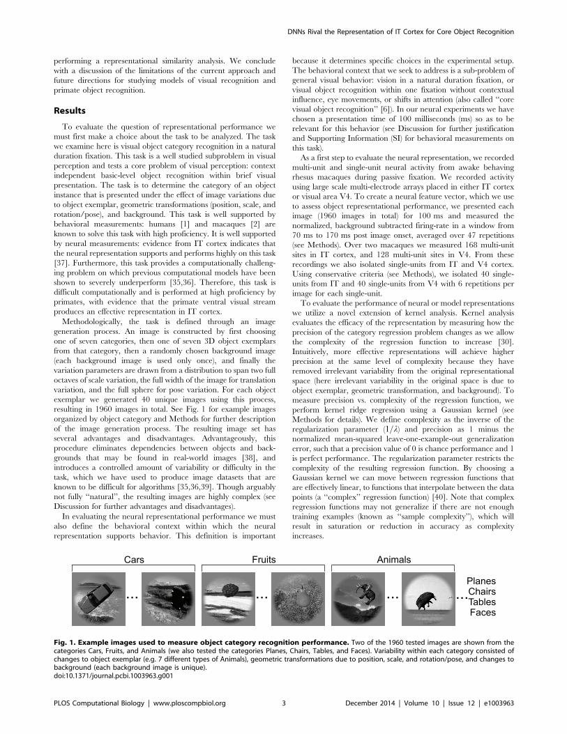
Methodologically, the task is defined through an imagegeneration process. An image is constructed by first choosingone of seven categories, then one of seven 3D object exemplarsfrom that category, then a randomly chosen background image(each background image is used only once), and finally thevariation parameters are drawn from a distribution to span two fulloctaves of scale variation, the full width of the image for translationvariation, and the full sphere for pose variation. For each objectexemplar we generated 40 unique images using this process,resulting in 1960 images in total. See Fig. 1 for example imagesorganized by object category and Methods for further descriptionof the image generation process. The resulting image set hasseveral advantages and disadvantages. Advantageously, thisprocedure eliminates dependencies between objects and back-grounds that may be found in real-world images [38], andintroduces a controlled amount of variability or difficulty in thetask, which we have used to produce image datasets that areknown to be difficult for algorithms [35,36,39]. Though arguablynot fully ‘‘natural’’, the resulting images are highly complex (seeDiscussion for further advantages and disadvantages).

In evaluating the neural representational performance we mustalso define the behavioral context within which the neuralrepresentation supports behavior. This definition is important

because it determines specific choices in the experimental setup.The behavioral context that we seek to address is a sub-problem ofgeneral visual behavior: vision in a natural duration fixation, orvisual object recognition within one fixation without contextualinfluence, eye movements, or shifts in attention (also called ‘‘corevisual object recognition’’ [6]). In our neural experiments we havechosen a presentation time of 100 milliseconds (ms) so as to berelevant for this behavior (see Discussion for further justificationand Supporting Information (SI) for behavioral measurements onthis task).

As a first step to evaluate the neural representation, we recordedmulti-unit and single-unit neural activity from awake behavingrhesus macaques during passive fixation. We recorded activityusing large scale multi-electrode arrays placed in either IT cortexor visual area V4. To create a neural feature vector, which we useto assess object representational performance, we presented eachimage (1960 images in total) for 100 ms and measured thenormalized, background subtracted firing-rate in a window from70 ms to 170 ms post image onset, averaged over 47 repetitions(see Methods). Over two macaques we measured 168 multi-unitsites in IT cortex, and 128 multi-unit sites in V4. From theserecordings we also isolated single-units from IT and V4 cortex.Using conservative criteria (see Methods), we isolated 40 single-units from IT and 40 single-units from V4 with 6 repetitions perimage for each single-unit.

To evaluate the performance of neural or model representationswe utilize a novel extension of kernel analysis. Kernel analysisevaluates the efficacy of the representation by measuring how theprecision of the category regression problem changes as we allowthe complexity of the regression function to increase [30].Intuitively, more effective representations will achieve higherprecision at the same level of complexity because they haveremoved irrelevant variability from the original representationalspace (here irrelevant variability in the original space is due toobject exemplar, geometric transformation, and background). Tomeasure precision vs. complexity of the regression function, weperform kernel ridge regression using a Gaussian kernel (seeMethods for details). We define complexity as the inverse of theregularization parameter (1=l) and precision as 1 minus thenormalized mean-squared leave-one-example-out generalizationerror, such that a precision value of 0 is chance performance and 1is perfect performance. The regularization parameter restricts thecomplexity of the resulting regression function. By choosing aGaussian kernel we can move between regression functions thatare effectively linear, to functions that interpolate between the datapoints (a ‘‘complex’’ regression function) [40]. Note that complexregression functions may not generalize if there are not enoughtraining examples (known as ‘‘sample complexity’’), which willresult in saturation or reduction in accuracy as complexityincreases.

Fig. 1. Example images used to measure object category recognition performance. Two of the 1960 tested images are shown from thecategories Cars, Fruits, and Animals (we also tested the categories Planes, Chairs, Tables, and Faces). Variability within each category consisted ofchanges to object exemplar (e.g. 7 different types of Animals), geometric transformations due to position, scale, and rotation/pose, and changes tobackground (each background image is unique).doi:10.1371/journal.pcbi.1003963.g001



We compared the neural representation to three convolutionalDNNs and three other biologically relevant representations. Notethat the development of these representations did not utilize the1960 images we use here for testing in any way. The three recentconvolutional DNNs we examine are described in Krizhevsky etal. 2012 [24], Zeiler & Fergus 2013 [25], and Yamins et al. 2014[27,34]. The Krizhevsky et al. 2012 and Zeiler & Fergus 2013DNNs are of note because they have each successively surpassedthe state-of-the-art performance on the ImageNet Large ScaleVisual Recognition Challenge (ILSVRC) datasets. Note thatresults have continued to improve on this challenge since we ranour analysis. See http://www.image-net.org/for the latest results.The DNN presented in Yamins et al. 2014 [27] is created using asupervised optimization procedure called hierarchical modularoptimization (we refer to this model by the abbreviation HMO).The HMO DNN has been shown to match closely representa-tional dissimilarity matrices of the ventral stream and to bepredictive of IT and V4 neural responses [27]. We also evaluatedan instantiation of the HMAX model of invariant objectrecognition that uses sparse localized features [41] and haspreviously been shown to be a relatively high performing modelamong artificial systems [16]. Finally, we also evaluated a V2-likemodel and a V1-like model that each attempt to capture a first-order account of secondary (V2) [42] and primary visual cortex(V1) [35], respectively.

Each of the three convolutional DNNs was developed,implemented, and trained by their respective researchers and forthose developed outside of our group we obtained features fromeach DNN computed on our test images. The convolutional DNNdescribed in Krizhevsky et al. 2012 [24] was trained by supervisedlearning on the ImageNet 2011 Fall release (,15 M images, 22Kcategories) with additional training on the LSVRC-2012 dataset(1000 categories). The authors computed the features in thepenultimate layer of their model (4096 features) on the 1960images we used to measure the neural representation. The similar8-layer deep neural network of Zeiler & Fergus 2013 [25] wastrained using supervised learning on the LSVRC-2012 datasetaugmented with random crops and left-right flips. This model tookadvantage of hyper-parameter tuning informed by visualizations ofthe intermediate network layers. The 4096 dimensional featurerepresentation was produced by taking the penultimate layerfeatures and averaging them over 10 image crops (the 4 corners,center, and horizontal flips for each). The model of Yamins et al.2014 [27] is an extension of the high-throughput optimizationstrategy described in [16] that produces a heterogeneouscombination of hierarchical convolutional models optimized ona supervised object recognition task through hyperparameteroptimization using boosting and error-based reweighing (see [27]for details). The total output feature space per image for the HMOmodel is 1250 dimensional.

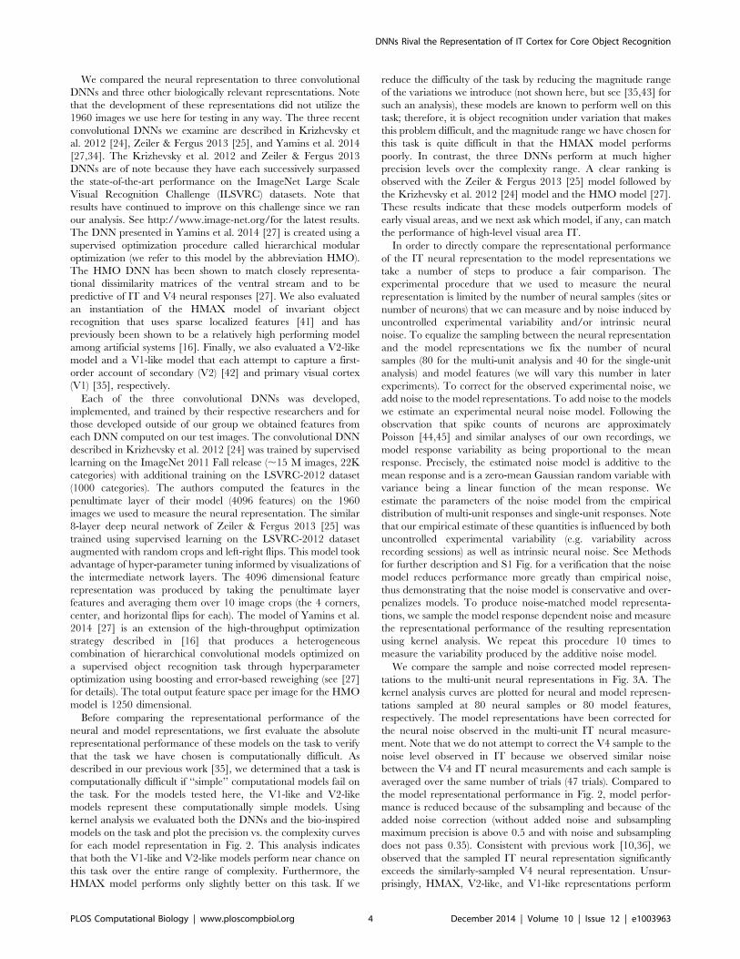
Before comparing the representational performance of theneural and model representations, we first evaluate the absoluterepresentational performance of these models on the task to verifythat the task we have chosen is computationally difficult. Asdescribed in our previous work [35], we determined that a task iscomputationally difficult if ‘‘simple’’ computational models fail onthe task. For the models tested here, the V1-like and V2-likemodels represent these computationally simple models. Usingkernel analysis we evaluated both the DNNs and the bio-inspiredmodels on the task and plot the precision vs. the complexity curvesfor each model representation in Fig. 2. This analysis indicatesthat both the V1-like and V2-like models perform near chance onthis task over the entire range of complexity. Furthermore, theHMAX model performs only slightly better on this task. If we

reduce the difficulty of the task by reducing the magnitude rangeof the variations we introduce (not shown here, but see [35,43] forsuch an analysis), these models are known to perform well on thistask; therefore, it is object recognition under variation that makesthis problem difficult, and the magnitude range we have chosen forthis task is quite difficult in that the HMAX model performspoorly. In contrast, the three DNNs perform at much higherprecision levels over the complexity range. A clear ranking isobserved with the Zeiler & Fergus 2013 [25] model followed bythe Krizhevsky et al. 2012 [24] model and the HMO model [27].These results indicate that these models outperform models ofearly visual areas, and we next ask which model, if any, can matchthe performance of high-level visual area IT.

In order to directly compare the representational performanceof the IT neural representation to the model representations wetake a number of steps to produce a fair comparison. Theexperimental procedure that we used to measure the neuralrepresentation is limited by the number of neural samples (sites ornumber of neurons) that we can measure and by noise induced byuncontrolled experimental variability and/or intrinsic neuralnoise. To equalize the sampling between the neural representationand the model representations we fix the number of neuralsamples (80 for the multi-unit analysis and 40 for the single-unitanalysis) and model features (we will vary this number in laterexperiments). To correct for the observed experimental noise, weadd noise to the model representations. To add noise to the modelswe estimate an experimental neural noise model. Following theobservation that spike counts of neurons are approximatelyPoisson [44,45] and similar analyses of our own recordings, wemodel response variability as being proportional to the meanresponse. Precisely, the estimated noise model is additive to themean response and is a zero-mean Gaussian random variable withvariance being a linear function of the mean response. Weestimate the parameters of the noise model from the empiricaldistribution of multi-unit responses and single-unit responses. Notethat our empirical estimate of these quantities is influenced by bothuncontrolled experimental variability (e.g. variability acrossrecording sessions) as well as intrinsic neural noise. See Methodsfor further description and S1 Fig. for a verification that the noisemodel reduces performance more greatly than empirical noise,thus demonstrating that the noise model is conservative and over-penalizes models. To produce noise-matched model representa-tions, we sample the model response dependent noise and measurethe representational performance of the resulting representationusing kernel analysis. We repeat this procedure 10 times tomeasure the variability produced by the additive noise model.

We compare the sample and noise corrected model represen-tations to the multi-unit neural representations in Fig. 3A. Thekernel analysis curves are plotted for neural and model represen-tations sampled at 80 neural samples or 80 model features,respectively. The model representations have been corrected forthe neural noise observed in the multi-unit IT neural measure-ment. Note that we do not attempt to correct the V4 sample to thenoise level observed in IT because we observed similar noisebetween the V4 and IT neural measurements and each sample isaveraged over the same number of trials (47 trials). Compared tothe model representational performance in Fig. 2, model perfor-mance is reduced because of the subsampling and because of theadded noise correction (without added noise and subsamplingmaximum precision is above 0.5 and with noise and subsamplingdoes not pass 0.35). Consistent with previous work [10,36], weobserved that the sampled IT neural representation significantlyexceeds the similarly-sampled V4 neural representation. Unsur-prisingly, HMAX, V2-like, and V1-like representations perform



near chance. All three recent DNNs perform better than the V4representation. The IT representation performs quite well,especially considering the sampling and noise limitations of ourrecordings and would be quite competitive if directly compared tothe model results in Fig. 2. After correcting for sampling andnoise, the IT representation is only matched by the top performingDNN of Zeiler & Fergus 2013. Interestingly, this relationship holdsfor the entire complexity range.

We present the equivalent representational comparison betweenmodels and neural representations for the single-unit neuralrecordings in Fig. 3B. Because of the increased noise and fewertrials collected for the single-unit measurements compared to ourmulti-unit measurements, the single-unit noise and samplecorrected model representations achieve lower precision vs.complexity curves than under the multi-unit noise and samplecorrection (compare to Fig. 3A). This analysis shows that thesingle-unit IT representation performs better than the HMOrepresentation, slightly worse than the Krizhevsky et al. 2012

representation, and is outperformed by the Zeiler & Fergus 2013[25] representation. Furthermore, a comparison of the relativeperformance of the multi-unit sample and the single-unit sampleindicates that the multi-unit sample outperforms the single-unitsample. See Discussion for elaboration of this finding and S4 Fig.for trial corrected performance comparison between single- andmulti-units.

In Figs. 4A and 4B we analyze the representational perfor-mance as a function of neural sites or model features for multi-unitand single-unit neural measurements. To achieve a summarynumber from the kernel analysis curves we compute the area-under-the-curve and we omit the HMAX, V2-like, and V1-likemodels because they are near zero performance in this regime. InFig. 4A we vary the number of multi-unit recording samples andthe number of features. Just as in Fig. 3A, we correct for neuralnoise by adding a matched neural noise level to the modelrepresentations. Fig. 4A indicates that the representationalperformance relationship we observed at 80 samples is robust

Fig. 2. Kernel analysis curves of model representations. Precision, one minus loss (1{looe(l)), is plotted against complexity, the inverse of theregularization parameter (1=l). Shaded regions indicate the standard deviation of the measurement over image set randomizations, which are oftensmaller than the line thickness. The Zeiler & Fergus 2013, Krizhevsky et al. 2012 and HMO models are all hierarchical deep neural networks. HMAX [41]is a model of the ventral visual stream and the V1-like [35] and V2-like [42] models attempt to replicate response properties of visual areas V1 and V2,respectively. These analyses indicate that the task we are measuring proves difficult for V1-like and V2-like models, with these models barely movingfrom 0.0 precision for all levels of complexity. Furthermore, the HMAX model, which has previously been shown to perform relatively well on objectrecognition tasks, performs only marginally better. Each of the remaining deep neural network models performs drastically better, with the Zeiler &Fergus 2013 model performing best for all levels of complexity. These results indicate that the visual object recognition task we evaluate iscomputationally challenging for all but the latest deep neural networks.doi:10.1371/journal.pcbi.1003963.g002



Fig. 3. Kernel analysis curves of sample and noise matched neural and model representations. Plotting conventions are the same as inFig. 2. Multi-unit analysis is presented in panel A and single-unit analysis in B. Note that the model representations have been modified such that theyare both subsampled and noisy versions of those analyzed in Fig. 2 and this modification is indicated by the { symbol for noise matched to the multi-unit IT cortex sample and by the { symbol for noise matched to the single-unit IT cortex sample. To correct for sampling bias, the multi-unit analysisuses 80 samples, either 80 neural multi-units from V4 or IT cortex, or 80 features from the model representations, and the single-unit analysis uses 40samples. To correct for experimental and intrinsic neural noise, we added noise to the subsampled model representation (no additional noise isadded to the neural representations) that is commensurate to the observed noise from the IT measurements. Note that we observed similar noisebetween the V4 and IT Cortex samples and we do not attempt to correct the V4 cortex sample of the noise observed in the IT cortex sample. Weobserved substantially higher noise levels in IT single-unit recordings than multi-unit recordings due to both higher trial-to-trial variability and moretrials for the multi-unit recordings. All model representations suffer decreases in accuracy after correcting for sampling and adding noise (compareabsolute precision values to Fig. 2). All three deep neural networks perform significantly better than the V4 cortex sample. For the multi-unit analysis(A), IT cortex sample achieves high precision and is only matched in performance by the Zeiler & Fergus 2013 representation. For the single-unitanalysis (B), both the Krizhevsky et al. 2012 and the Zeiler & Fergus 2013 representations surpass the IT representational performance.doi:10.1371/journal.pcbi.1003963.g003

Fig. 4. Effect of sampling the neural and noise-corrected model representations. We measure the area-under-the-curve of the kernelanalysis measurement as we change the number of neural sites (for neural representations), or the number of features (for model representations).Measured samples are indicated by filled symbols and measured standard deviations indicated by error bars. Multi-unit analysis is shown in panel Aand single-unit analysis in B. The model representations are noise corrected by adding noise that is matched to the IT multi-unit measurements (A, asindicated by the { symbol) or single-unit measurements (B, as indicated by the { symbol). For the multi-unit analysis, the Zeiler & Fergus 2013representation rivals the IT cortex representation over our measured sample. For the single-unit analysis, the Krizhevsky et al. 2012 representationrivals the IT cortex representation for low number of features and slightly surpasses it for higher number of features. The Zeiler & Fergus 2013representation surpasses the IT cortex representation over our measured sample.doi:10.1371/journal.pcbi.1003963.g004



between 10 samples and 160 samples. Fig. 4B indicates that theperformance of the IT single-unit representation is comparativelyworse than the multi-unit, with the single-unit representationfalling below the performance of the Krizhevsky et al. 2012representation for much of the range of our analysis.

These results indicate that after correcting for noise andsampling effects, the Zeiler & Fergus 2013 DNN rivals theperformance of the IT multi-unit representation and that both theKrizhevsky et al. 2012 and Zeiler & Fergus 2013 DNNs surpassesthe performance of the IT single-unit representation. Theperformance of these two DNNs in the low-complexity regime isespecially interesting because it indicates that they performcomparably to the IT representation in the low-sample regime(i.e. low number of training examples), where restricted represen-tational complexity is essential for generalization (e.g. [46]).

To verify the results of the kernel analysis procedure wemeasured linear-SVM generalization performance on the sametask for each neural and model representation (Fig. 5). We used across-validated procedure to train the linear-SVM on 80% of theimages and test on 20% (regularization parameters were estimatedfrom the training set). We repeated the procedure for 10randomizations of the training-testing split. The linear-SVMresults reveal a similar relationship to the results produced usingkernel analysis (Fig. 3A). This indicates that the Zeiler & Fergus2013 representation achieves generalization comparable to the ITmulti-unit neural sample for a simple linear decision boundary.We also found near identical results to kernel analysis for the

single-unit analyses and the analysis of performance as a functionof the number of neural sites or features (see S4 Fig.).

While the goal of our analysis has been to measure represen-tational performance of neural and machine representations it isalso informative to measure neural encoding metrics and measuresof representational similarity. Such analyses are complementarybecause representational performance relates to the task goals (inthis case category labels) and encoding models and representa-tional similarity metrics are informative about a model’s ability tocapture image-dependent neural variability, even if this variabilityis unrelated to task goals. We measured the performance of themodel representations as encoding models of the IT multi-unitresponses by estimating linear regression models from the modelrepresentations to the IT multi-unit responses. We estimatedmodels on 80% of the images and tested on 20%, repeating theprocedure 10 times (see Methods). The median predictionsaveraged over the 10 splits are presented in Fig. 6A. Forcomparison, we also estimated regression models using the V4multi-unit responses to predict IT multi-unit responses. The resultsshow that the Krizhevsky et al. 2012 and the Zeiler & Fergus 2013DNNs achieve higher prediction accuracies than the HMO model,which was previously shown to achieve high predictions on asimilar test [27]. These predictions are similar in explainedvariance to the predictions achieved by V4 multi-units. However,no model is able to fully account for the explainable variance inthe IT multi-unit responses. In Fig. 6B we show the meanexplained variance of each IT multi-unit site as predicted by the

Fig. 5. Linear-SVM generalization performance of neural and model representations. Testing set classification accuracy averaged over 10randomly-sampled test sets is plotted and error bars indicate standard deviation over the 10 random samples. Chance performance is ,14.3%. V4and IT Cortex Multi-Unit Sample are the values measured directly from the neural samples. Following the analysis in Fig. 3A, the modelrepresentations have been modified such that they are both subsampled and have noise added that is matched to the observed IT multi-unit noise.We indicate this modification by the { symbol. Both model and neural representations are subsampled to 80 multi-unit samples or 80 features.Mirroring the results using kernel analysis, the IT cortex multi-unit sample achieves high generalization accuracy and is only matched in performanceby the Zeiler & Fergus 2013 representation.doi:10.1371/journal.pcbi.1003963.g005



V4 cortex multi-unit sample and the Zeiler & Fergus 2013 DNN.There is a relatively weak relationship between the encodingperformance of the neural V4 and DNN representations (r = 0.48between V4 and Zeiler & Fergus 2013, compared to r = 0.96 andr = 0.74 for correlations between Krizhevsky et al. 2012 and Zeiler& Fergus 2013, and HMO and Zeiler & Fergus 2013,respectively), indicating that V4 and DNN representations mayaccount for different sources of variability in IT (see Discussion).

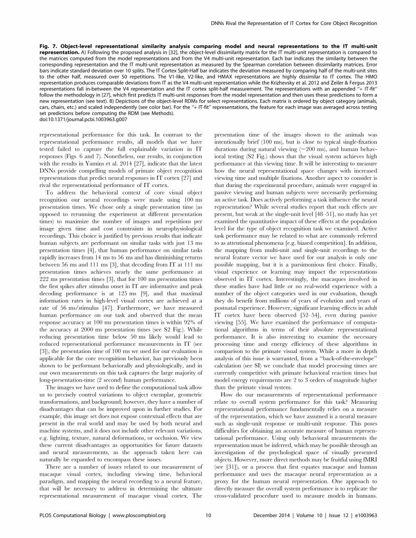
Finally, we measured representational similarity using theanalysis methodology proposed in [32]. This analysis methodologymeasures how similar two representations are and is robust toglobal scalings and rotations of the representational spaces. Tocompute the representational similarity between the IT multi-unitand model representations, we computed object-level representa-tional dissimilarity matrices (RDMs) for model and neuralrepresentations (matrices are 49x49 dimensional as there are 49total objects). We then measured the Spearman rank correlationsbetween the model derived RDM and the IT multi-unit RDM (seeMethods). In Fig. 7A we show the results of the representationalsimilarity measurements for the model representations and inFig. 7B we show depictions of the RDMs for select representa-tions. For comparison we present the result between the V4 multi-unit representation and the IT multi-unit representation. Todetermine the variability due to the IT neural sample, we alsopresent the similarity measurement between one-half of the ITmulti-units and the other half (IT Cortex Split-Half). In addition,we provide results following the methodology in [27], which firstpredicts the IT multi-unit site responses from the modelrepresentation and then uses these predictions to form a newrepresentation. We refer to these representations with anappended ‘‘+IT-fit’’. Our measurements of the HMO + IT-fitrepresentation are in general agreement with the results in [27] butvary slightly because of differences in the image set used toproduce these measurements and details of the methodology usedto produce the IT predictions. Interestingly, by fitting a lineartransform at the image-level to IT multi-units, the Krizhevsky etal. 2012 and Zeiler & Fergus 2013 DNNs fall within the noise limit

of the IT split-half object-level RDM measurement. However, theHMO, Krizhevsky et al. 2012, and Zeiler & Fergus 2013representations, without the added linear mapping, have devia-tions from the IT representation that are unexplained by noisevariation. While it is informative that a linear mapping canproduce RDMs in correspondence with the IT RDM, weconclude that there remains a gap between DNN models andIT representation when measured with object-level representa-tional similarity.

Discussion

In summary, our measurements indicate that the latest DNNsrival the representational performance of IT cortex on a rapidobject category recognition task. We evaluated representationalperformance using a novel kernel analysis methodology, whichmeasures precision as a function of classifier complexity. Kernelanalysis allows us to measure a desirable property of arepresentation: a good representation is highly performant with asimple classification function and can thus accurately predict classlabels from few examples, while a poor representation is onlyperformant with complex classification functions and thus requiresa large number of training examples to accurately predict (seeMethods for elaboration on this point). Importantly, we madecomparisons between models and neural measurements bycorrecting the models for experimental limitations due tosampling, noise, and trials. In this analysis we found that theZeiler & Fergus 2013 DNN achieved comparable representationalperformance to the IT cortex multi-unit representation and boththe Krizhevsky et al. 2012 and Zeiler & Fergus 2013 represen-tations surpassed the performance of the IT cortex single-unitrepresentation. These results reflect substantial progress ofcomputational object recognition systems since our previousevaluations of model representations using a similar objectrecognition task [35,36]. These results extend our understandingover recent, complimentary studies, which have examinedrepresentational similarity [27], by evaluating directly absolute

Fig. 6. Neural and model representation predictions of IT multi-unit responses. A) The median predictions of IT multi-unit responsesaveraged over 10 train/test splits is plotted for model representations and V4 multi-units. Error bars indicate standard deviation over the 10 train/testsplits. Predictions are normalized to correct for trial-to-trial variability of the IT multi-unit recording and calculated as percentage of explained,explainable variance. The HMO, Krizhevsky et al. 2012, and Zeiler & Fergus 2013 representations achieve IT multi-unit predictions that are comparableto the predictions produced by the V4 multi-unit representation. B) The mean predictions over the 10 train/test splits for the V4 cortex multi-unitsample and the Zeiler & Fergus 2013 DNN are plotted against each other for each IT multi-unit site.doi:10.1371/journal.pcbi.1003963.g006



representational performance for this task. In contrast to therepresentational performance results, all models that we havetested failed to capture the full explainable variation in ITresponses (Figs. 6 and 7). Nonetheless, our results, in conjunctionwith the results in Yamins et al. 2014 [27], indicate that the latestDNNs provide compelling models of primate object recognitionrepresentations that predict neural responses in IT cortex [27] andrival the representational performance of IT cortex.

To address the behavioral context of core visual objectrecognition our neural recordings were made using 100 mspresentation times. We chose only a single presentation time (asopposed to rerunning the experiment at different presentationtimes) to maximize the number of images and repetitions perimage given time and cost constraints in neurophysiologicalrecordings. This choice is justified by previous results that indicatehuman subjects are performant on similar tasks with just 13 mspresentation times [4], that human performance on similar tasksrapidly increases from 14 ms to 56 ms and has diminishing returnsbetween 56 ms and 111 ms [3], that decoding from IT at 111 mspresentation times achieves nearly the same performance at222 ms presentation times [3], that for 100 ms presentation timesthe first spikes after stimulus onset in IT are informative and peakdecoding performance is at 125 ms [9], and that maximalinformation rates in high-level visual cortex are achieved at arate of 56 ms/stimulus [47]. Furthermore, we have measuredhuman performance on our task and observed that the meanresponse accuracy at 100 ms presentation times is within 92% ofthe accuracy at 2000 ms presentation times (see S2 Fig.). Whilereducing presentation time below 50 ms likely would lead toreduced representational performance measurements in IT (see[3]), the presentation time of 100 ms we used for our evaluation isapplicable for the core recognition behavior, has previously beenshown to be performant behaviorally and physiologically, and inour own measurements on this task captures the large majority oflong-presentation-time (2 second) human performance.

The images we have used to define the computational task allowus to precisely control variations to object exemplar, geometrictransformations, and background; however, they have a number ofdisadvantages that can be improved upon in further studies. Forexample, this image set does not expose contextual effects that arepresent in the real world and may be used by both neural andmachine systems, and it does not include other relevant variations,e.g. lighting, texture, natural deformations, or occlusion. We viewthese current disadvantages as opportunities for future datasetsand neural measurements, as the approach taken here cannaturally be expanded to encompass these issues.

There are a number of issues related to our measurement ofmacaque visual cortex, including viewing time, behavioralparadigm, and mapping the neural recording to a neural feature,that will be necessary to address in determining the ultimaterepresentational measurement of macaque visual cortex. The

presentation time of the images shown to the animals wasintentionally brief (100 ms), but is close to typical single-fixationdurations during natural viewing (,200 ms), and human behav-ioral testing (S2 Fig.) shows that the visual system achieves highperformance at this viewing time. It will be interesting to measurehow the neural representational space changes with increasedviewing time and multiple fixations. Another aspect to consider isthat during the experimental procedure, animals were engaged inpassive viewing and human subjects were necessarily performingan active task. Does actively performing a task influence the neuralrepresentation? While several studies report that such effects arepresent, but weak at the single-unit level [48–51], no study has yetexamined the quantitative impact of these effects at the populationlevel for the type of object recognition task we examined. Activetask performance may be related to what are commonly referredto as attentional phenomena [e.g. biased competition]. In addition,the mapping from multi-unit and single-unit recordings to theneural feature vector we have used for our analysis is only onepossible mapping, but it is a parsimonious first choice. Finally,visual experience or learning may impact the representationsobserved in IT cortex. Interestingly, the macaques involved inthese studies have had little or no real-world experience with anumber of the object categories used in our evaluation, thoughthey do benefit from millions of years of evolution and years ofpostnatal experience. However, significant learning effects in adultIT cortex have been observed [52–54], even during passiveviewing [55]. We have examined the performance of computa-tional algorithms in terms of their absolute representationalperformance. It is also interesting to examine the necessaryprocessing time and energy efficiency of these algorithms incomparison to the primate visual system. While a more in depthanalysis of this issue is warranted, from a ‘‘back-of-the-envelope’’calculation (see SI) we conclude that model processing times arecurrently competitive with primate behavioral reaction times butmodel energy requirements are 2 to 3 orders of magnitude higherthan the primate visual system.

How do our measurements of representational performancerelate to overall system performance for this task? Measuringrepresentational performance fundamentally relies on a measureof the representation, which we have assumed is a neural measuresuch as single-unit response or multi-unit response. This posesdifficulties for obtaining an accurate measure of human represen-tational performance. Using only behavioral measurements therepresentation must be inferred, which may be possible through aninvestigation of the psychological space of visually presentedobjects. However, more direct methods may be fruitful using fMRI(see [31]), or a process that first equates macaque and humanperformance and uses the macaque neural representation as aproxy for the human neural representation. One approach todirectly measure the overall system performance is to replicate thecross-validated procedure used to measure models in humans.

Fig. 7. Object-level representational similarity analysis comparing model and neural representations to the IT multi-unitrepresentation. A) Following the proposed analysis in [32], the object-level dissimilarity matrix for the IT multi-unit representation is compared tothe matrices computed from the model representations and from the V4 multi-unit representation. Each bar indicates the similarity between thecorresponding representation and the IT multi-unit representation as measured by the Spearman correlation between dissimilarity matrices. Errorbars indicate standard deviation over 10 splits. The IT Cortex Split-Half bar indicates the deviation measured by comparing half of the multi-unit sitesto the other half, measured over 50 repetitions. The V1-like, V2-like, and HMAX representations are highly dissimilar to IT cortex. The HMOrepresentation produces comparable deviations from IT as the V4 multi-unit representation while the Krizhevsky et al. 2012 and Zeiler & Fergus 2013representations fall in-between the V4 representation and the IT cortex split-half measurement. The representations with an appended ‘‘+ IT-fit’’follow the methodology in [27], which first predicts IT multi-unit responses from the model representation and then uses these predictions to form anew representation (see text). B) Depictions of the object-level RDMs for select representations. Each matrix is ordered by object category (animals,cars, chairs, etc.) and scaled independently (see color bar). For the ‘‘+ IT-fit’’ representations, the feature for each image was averaged across testingset predictions before computing the RDM (see Methods).doi:10.1371/journal.pcbi.1003963.g007



Such a procedure should control the human exposure to thetraining set and provide the correct labels on the training set. Theprocedure for measuring human performance presented in the SIdoes not follow this procedure. However, a comparison betweenhuman performance at 100 ms presentation times (see S2 Fig.) andoverall DNN model performance on the test-set (see S3 Fig.)indicates that there is likely a gap between human performance(85% mean accuracy) and DNN performance (77% meanaccuracy) on this task because allowing the human subjectsexposure to 80% of the images with the correct labels is only likelyto increase the human performance number. Furthermore, there isindividual variability in the human performance with someindividuals performing well above the mean. Therefore, whilewe have not attempted to make a direct comparison betweenhuman performance and DNN performance, we infer that humanperformance exceeds current DNN performance.

Our methodology and approach relates to the encoding anddecoding approaches in systems neuroscience, which, in our view,provide complementary insights into neural visual processing. Thekernel analysis methodology we use here is a neural decodingapproach because it measures the relationship between the neural(or model) representation and unobserved characteristics of thestimuli (class labels). The linear-SVM methodology is also adecoding approach because it tests the generalization performanceof predicting the unobserved class label from the neural (or model)representation. The approaches of predicting IT multi-unitresponse (Fig. 6) and measuring representational similarity to ITrepresentation (Fig. 7) are encoding approaches because theymeasure the relationship between functions or measurementsderived from the stimuli (pixels in the images) and the neuralvariation present in IT. The complementary nature of theseapproaches is demonstrated in our results. For example, while theZeiler & Fergus 2013 DNN rivals the decoding performance of ITcortex, it fails to capture over 40% of the explainable variance inthe IT neural sample and therefore does not produce a completeneural encoding model. Conversely, the V4 multi-unit represen-tation severely underperforms the DNNs and IT cortex whenmeasured with decoding approaches but produces comparableresults to these representations when predicting IT multi-unitresponses with an encoding approach. It is currently unclear whatvariation in the IT cortex multi-unit representation is not capturedby DNNs or the V4 multi-unit representation. Furthermore, theIT variation that is captured by DNNs and V4 is, relative tocorrelations between DNN models, weakly correlated (Fig. 6B).Overall, the remaining unexplained IT variation may be exposedthrough a decoding approach (by, for example, exploringadditional task labels), through an encoding approach (byexploring additional stimulus transformations), or through ap-proaches that take into account intrinsic neural dynamics (e.g.[56]). The comparably high performance of the V4 multi-unitrepresentation at predicting IT multi-unit responses may be due toits ability to capture intrinsic neural dynamics present in IT thatare unrelated to stimulus derived variables.

We found that multi-units outperform single-units in ourevaluation, as evidenced in the relative performance increase ofDNNs over single-units in Figs. 3 and 4 and in a trial correctedcomparison between multi- and single-units in S4 Fig. It may besurprising that multi-units outperform single-units on this task. Apriori, we might assume that the averaging process introduced bythe multi-unit recording, which aggregates the spikes frommultiple spatially-localized single-units, would ‘‘wash-out’’ oraverage away neural selectivity for visual objects. However, whenconsidering generalization performance, it is possible that aver-aged single-units could outperform the original single-units by

removing noise or non-class specific signal variation. In this way,multi-units may provide a form of regularization that isappropriate for this task. This regularization may be due toaveraging out single-unit noise, and/or reducing variation in therepresentational space that is irrelevant, and therefore spurious, forthe task. Alternatively, the single-unit variation may be appropri-ate for different tasks that we have not measured, such as finedistinctions between objects or 3-dimensional object surfacerepresentation. The spatial arrangement of functional corticalresponses (topographic maps, and functional clustering) alsoindicates a current limitation of DNNs as models of high-levelvisual cortex. There is no notion of tissue or cortical space in theDNN layers that we utilize as features: the features correspond tofully connected layers which do not have convolutional topology,which may be trivially mapped to physical space, nor do they havelocalized operations, such as local divisive normalization. For thisreason, it is non-trivial to include a biologically realistic averagingprocess to the DNN representations.

Could the regularizing properties of multi-unit responses beindicative of broader regularization mechanisms related to spatialorganization in cortex (topographic maps, and functional cluster-ing)? Just as our multi-unit recordings average together a numberof single-units, neurons ‘‘reading-out’’ signals from IT cortex couldaverage over cortical topography and thus regularize theclassification decision boundary. This suggests the future goal offinding an appropriate mapping of biological phenomenology andphysical mechanism to the computational concepts of kernels,regularizers, and representational spaces. The overall performanceof learning algorithms strongly depends on the interconnectionsbetween the choice of kernel, regularizer, and representation. Inour current work (and the predominant mode in the field), we havemade specific choices on the kernel and regularizer and examinedaspects of the representational space. However, a full account ofbiological learning and decision making must determine accuratedescriptions for all three of these computational components inbiological systems.

Interestingly, many of the computational concepts utilized in thehigh performing DNNs that we have measured extend back toearly models of the primate visual system. All three DNNs weexamined [24,25,27] implement architectures containing succes-sive layers of operations that resemble the simple and complex cellhierarchy first described by Hubel and Wiesel [17,18]. Inparticular, max-pooling was proposed in [13] and is a prominentfeature of all three DNNs. Additional computational concepts areconvolution or weight sharing, which was introduced in [57] andutilized in [24,25], and backpropagation [58], which is utilized in[24,25].

The success of the Krizhevsky et al. 2012 and the Zeiler &Fergus 2013 DNNs raises a number of interesting questions. Thecategories we used for testing (the 7 classes used in the kernelanalysis measurements) are a small fraction of the 1000 classes thatthese models were trained on, and it is not clear if there is a directcorrespondence between the classes in the two image sets. At thispoint it is not clear how the non-relevant classes in the set used totrain the models affects our performance estimate. As moredetailed analyses are conducted it will be interesting to determinewhich categories are necessary to replicate ventral streamperformance and similarity. For example, there may be biases inthe necessary category distribution toward ecologically relevantcategories, such as faces. Of biological relevance, it is not clear ifnatural primate development is comparable to the 15M labeledimages used to train these DNNs and it seems likely that moreinnate knowledge of the visual world (acquired during evolution)and/or more unsupervised training (during development) are



utilized in biological systems. Finally, given their similar architec-tures, it is unclear why some DNNs perform well and others donot. However, our analyses provide cursory evidence that modelswith more layers perform better and models that effectively reducethe dimensionality of the original problem perform better. Morework is necessary to determine best practices using thesearchitectures and to determine the importance of hierarchicalrepresentations and representations that reduce dimensionality.The principled approach we have provided here allows forpractical evaluations between models and neurons, and mayprovide a tool in assessing progress in the development of DNNs.Going forward, we would ideally like a better theoreticalunderstanding of these architectures that would lead to moreconsistent implementations and would produce a detailed,mechanistic hypothesis for ventral stream processing (see [59] foran example of such an effort).

Methods

Ethics statementThis study was performed in strict accordance with the

recommendations in the Guide for the Care and Use ofLaboratory Animals of the National Institutes of Health. Allsurgical and experimental procedures were approved by theMassachusetts Institute of Technology Committee on AnimalCare (Animal protocol: 0111-003-014). All human behavioralmeasurements were approved by the Massachusetts Institute ofTechnology’s Committee on the Use of Humans as ExperimentalSubjects (number: 0812003043).

Image dataset generationSynthetic images of objects were generated using POV-Ray, a

free, high-quality ray tracing software package (http://www.povray.org). 3-d models (purchased from Dosch Design andTurboSquid) were converted to the POV-Ray format. Thisgeneral approach allowed us to generate image sets with arbitrarynumbers of different objects, undergoing controlled ranges ofidentity preserving object variation/transformation. The 2-dprojection of the 3-d model was then combined with a randomlychosen background. In our image set, no two images had the samebackground, in some cases the background was, by chance,correlated with the object (plane on a sky background, car on astreet) but more often they were uncorrelated, giving noinformation about the identity of the object. A circular aperturewith radial fall-off was applied to create each final image.

Neural data collectionWe collected neural data from V4 and IT across two adult male

rhesus monkeys (Macaca mulatta, 7 and 9 kg) by using a multi-electrode array recording system (BlackRock Microsystems,Cerebus System). We chronically implanted three arrays peranimal and recorded the 128 most visually driven neuralmeasurement sites (determined by separate pilot images) in oneanimal (58 IT, 70 V4) and 168 in another (110 IT, 58 V4). Duringimage presentation we recorded multi-unit neural responses to ourimages from the V4 and IT sites. Images were presented on anLCD screen (Samsung, SyncMaster 2233RZ at 120 Hz) one at atime. Each image was presented for 100 ms with a diameter of 8u(visual angle) at the center of the screen on top of the half-graybackground and was followed by a 100 ms half-gray ‘‘blank’’period. The animal’s eye position was monitored by a video eyetracking system (SR Research, EyeLink II), and the animal wasrewarded upon the successful completion of 6–8 image presenta-tions while maintaining good eye fixation (within 62u) at the

center of the screen, indicated by a small (0.25u) red dot.Presentations with larger eye movements were discarded. In eachexperimental block, we recorded responses to all images. Withinone block each image was repeated once. Over all recordingsessions, this resulted in the collection of 47 image repetitions,collected over multiple days. All surgical and experimentalprocedures were done in accordance with the National Instituteof Health guidelines and the Massachusetts Institute of Technol-ogy Committee on Animal Care.

To arrive at the multi-unit neural representation, we convertedthe raw multi-unit neural responses to a neural representationthrough the following normalization process. For each image in ablock, we compute the vector of raw firing rates acrossmeasurement sites by counting the number of spikes between70 ms and 170 ms after the onset of the image for each site. Wethen subtracted the background firing rate, which is the averagefiring rate during presentation of a gray background (‘‘blank’’image), from the evoked response. In order to minimize the effectof variable external noise, we normalize each site by the standarddeviation of each site’s response to a block of images. Finally, theneural representation is calculated by taking the mean across therepetitions for each image and for each site, producing a scalarvalued matrix of neural sites by images. This post-processingprocedure is only our current best-guess at a neural code, whichhas been shown to quantitatively account for human performance[60]. Therefore, it may be possible to develop a more effectiveneural decoding for example influenced by intrinsic corticalvariability [56], or dynamics [61,62].

To arrive at the single-unit neural representation, we followed asimilar normalization process as the multi-unit representation, butfirst conducted spike-sorting on the multi-unit recordings. Wesorted single-units from the multi-unit IT and V4 data by usingaffinity propagation [63] together with the method described in[64]. Using a conservative criteria we isolated 160 single-unitsfrom the IT recordings and 95 single-units from the V4 recordingswith 6 repetitions per image for each single-unit. Given thesesingle-unit responses for each image we followed a processingprocedure identical to the multi-unit procedure, which includedcounting the number of spikes between 70 ms and 170 ms afterthe onset of the image, subtracting the background firing rate, andnormalizing by the standard deviation of the site’s response to ablock of images. Finally, we selected from these single-units the top40 based on response consistency over trials on a separate imageset (units with high SNR). Specifically, we measured theresponse to 280 images not included in our evaluations ofperformance but drawn from a similar stimulus distribution.These images contained 7 unique objects not contained in theoriginal set with 1 object from each of the 7 categories. For eachobject there are 40 images, each with a unique background andwith the object position, scale, and pose randomly sampled. Foreach single-unit, we separated the responses over trials into twogroups, averaged across trials, and measured the correlation ofthese response vectors. We then sorted the single-units based onthis correlation and selected the 40 with highest correlation andtherefore most consistent single-units. We repeated this proce-dure separately for V4 and IT. The resulting consistencymeasurement for the IT single-units was comparable to othermeasurements using single-unit electrophysiology [10]. Theconsistency of the 40 IT single-units was higher than the 15thpercentile of single-units measured in [10]. In other words, theleast consistent IT single-unit in the group of 40 was moreconsistent than the bottom 15% of single-units analyzed in [10].Unless otherwise noted, all analyses of single-units use these 40high-SNR single-units.



Kernel analysis methodologyWe would also like to measure accuracy as we change the

complexity of the prediction function. To accomplish this, we usean extension of the work presented in [30], which is based ontheory presented in [28], and [29], and we refer to as kernelanalysis. We provide a brief description of this measure and referthe reader to those references for additional details andjustification on measuring precision against complexity. Thisprocedure is a derivative of regularized least squares [65], whicharrises as a Tikhonov minimization problem [46], and can beviewed as a form of Gaussian process regression [66]. We do notelaborate on the relationships between these views, but each is avalid interpretation on the procedure.

The measurement procedure, which we refer to here as kernelanalysis, utilizes regularized kernel ridge regression to determinehow well a task in question can be solved by a regularized kernel.A highly regularized kernel will allow only a simple predictionfunction in the feature space, and a weakly regularized kernel willallow a complex prediction function in the feature space. A goodrepresentation will have high variability in relation to the task inquestion and can effectively perform the task even under highregularization. Therefore, if the eigenvectors of the kernel with thelargest eigenvectors are effective at predicting the categories, ahighly regularized kernel will still be effective for that task. Incontrast, an ineffective representation will have very little variationrelevant for the task in question and variation relevant for the taskis only contained in the eigenvectors corresponding to the smallesteigenvalues of the kernel and only a weakly regularized kernel willbe capable of performing the task efficiently. Changing theamount of regularization changes the complexity of the resultingdecision function: highly regularized kernels allow for only simpledecision functions in the feature space and weakly regularizedkernels allow for complex decision functions. Intuitively, a goodrepresentation is one that learns a simple boundary (highlyregularized) from a small number of randomly-chosen examples,while a poor representation makes a more complicated boundary(weakly regularized), requiring many examples to do so.

In our formulation, kernel analysis consists of solving aregularized least squares or equivalently a kernel regressionproblem over a range of regularization [65]. The regularizationparameter l controls the complexity of the function and theprecision or performance is measured as the leave-one-outgeneralization error (looe). We refer to the inverse of theregularization parameter (1=l) as the complexity and 1{looe(l)as the precision. Thus, the curve 1{looe(l) provides us with ameasurement of the precision as a function of the modelcomplexity for the given representational space. The curvesproduced by different representational spaces will inform us aboutthe simplicity of the task in that representational space, with highercurves indicating that the problem is simpler for the representa-tion.

One of the advantages of kernel analysis is that the kernel PCAmethod converges favorably from a limited number of samples.[29] shows that the kernel PCA projections obtained with a finiteand typically small number of samples n (images in our context)are close with multiplicative errors to those that would be obtainedin the asymptotic case where n.?. This result is especiallyimportant in our setting as the number of images we canreasonably obtain from the neural measurements is comparativelylow. Therefore, kernel analysis provides us with a methodology forassessing representational effectiveness that has favorable proper-ties in the low image sample regime, here thousands of images.

We next present the specific computational procedure forcomputing kernel analysis. Given the learning problem p(x,y) and

a set of n data points f(x1,y1),:::,(xn,yn)g drawn independentlyfrom p(x,y) we evaluate a representation defined as a mappingx.w(x). For our case, the inputs x are images, the y arenormalized category labels, and the w denotes a feature extractionprocess.

As suggested by [30], we utilize the Gaussian kernel because thiskernel implies a smoothness of the task of interest in the inputspace [67] and does not bias against representations that may bemore adapted to non-linear regression functions. We compute thekernel matrix Ks associated to the data set as

Ks~

ks(w(x1),w(x1)) ::: ks(w(x1),w(xn))

..

. ...

ks(w(xn),w(x1)) ::: ks(w(xn),w(xn))

0

BBBB@

1

CCCCA, ð1Þ

where the standard Gaussian kernel is defined as

ks(x,x’)~ exp ({DDx{x’DD2=2s2) with scale parameter s.The regularized kernel regression problem is

minH[Rn1

2

Xn

i~1

EY{KsHE22z

l

2HtKsH, ð2Þ

where Y are the normalized vector of category labels, H is thevector of regression parameters and l is the regularization scalar.The solution to the regularized regression problem for a fixed sand l is denoted as Hs(l) and is given as

H#s(l)~(KszlI){1Y , ð3Þ

where I is the identity matrix.The leave-one-out error can be calculated as

LOOEs(l)~H#s(l)

diag((KszlI){1), ð4Þ

where diag(M) denotes the column vector satisfyingdiag(M)i~Mii and the division is elementwise. Note thatLOOEs(l) is a vector of errors for each example and wecompute the mean squared error over the examples as

looes(l)~1

n

Xi(LOOEs(l)i)

2, which is considered a good

empirical proxy for the error on future examples (generalizationerror). We note that the leave-one-out error can be computedefficiently given an eigendecomposition of the kernel matrix. Werefer to [65] for derivation and details on this computation.

To remove the dependence of the kernel on s we find the valuethat minimizes looes(l) at that value of l: looe(l)~minslooes(l).Finally, for convenience we plot precision (1{looe(l)) againstcomplexity (1=l). Note that because we optimize the value of s foreach value of complexity, s (the width of the Gaussian kernel) willregularize the feature space when l does not provide sufficientregularization. Because of this effect, the precision-complexitycurves in Fig. 2 plateau at high values of complexity because theoptimal value of s increases in the high complexity regime (lowvalues of l). We would otherwise expect that at high complexity,the regression would over fit and produce poor generalization (low1{looe(l) or high error). At low values of complexity (l) weobserve that there is an optimal value for s, which is dependent onthe representation, and is robust over image splits. Therefore, it isnot possible to achieve high precision at low complexity simply by



reducing s; the variation in the representational space must bealigned with the task in order to achieve high precision at lowcomplexity.

Note that we have chosen to use a squared error loss function forour multi-way classification problem. While it might be moreappropriate to evaluate a multi-way logistic loss function, we havechosen to use the least-squares loss because it provides a strongerrequirement on the representational space to reduce variance withincategory and to increase variance between categories, and it allowsus to distinguish representations that may be identical in terms ofseparability for a certain complexity but still have differences in theirfeature mappings. The kernel analysis of deep Boltzmann machinesin [68] also uses a mean squared loss function in the classificationproblem setting and is widely used in machine learning.

In the discussion above, Y~(y1, . . . ,yn) represents the vector oftask labels for the images (x1, . . . ,xn). In our specific case, the yi

are normalized category identity values (normalized such thatpredicting 0 will result in a precision equal to 0 and perfectprediction will result in a precision equal to 1). To generalize to thecase of multiway categorization, we use a version of the commonone-versus-all strategy. Assuming k distinct categories, for each

category j we compute the per-class leave-one-out error looes(l)j

by replacing Y in equations 2 and 3 with Yj . The overall leave-

one-out error is then the average over categories of the per-category leave-one-out error. Minimization over s then proceedsas in the single category case.

To evaluate both neural representations and machine repre-sentations using kernel analysis we measure the 1{looe(l) curve.The image dataset consists of 1960 images containing seven objectcategories with seven instances per object category. The categoriesare Animals, Cars, Chairs, Faces, Fruits, Planes and Tables. Tomeasure statistical variation due to subsampling of image variationparameters we compute the 1{looe(l) curve ten times, each timesampling 80% of the images with replacement. The ten samplesare fixed for all representations and within each subset we equalizethe number of images from each category. For each representa-tion, we maximize over the values of the Gaussian kernel sparameter as follows. We evaluate the Gaussian kernel scaleparameter s for each representation at a range of values centeredon the median distance over the distribution of distances for thatrepresentation. With sm denoting the value equal to the mediandistance, we evaluated kernels with s~asm for 32 values of a inthe range of 0:1 to 10 with logarithmic spacing. We found that inpractice the values of s that minimized the leave-one-out errorwere close to sm and well within this range. To span a large range

of complexity we evaluate looe(l) at 56 values of l from 10{4 to

103 with logarithmic spacing. For each representation, thisprocedure produces a curve for each of the subsets, where themean and spread (range of the values over the 10 subsets for eachvalue of l) are shown in Fig. 2. As a summary value, we alsocompute the area under the curve (KA-AUC) for each of theimage set randomizations and report the mean and standarddeviation. We use these mean KA-AUC values for the measure-ments in Figs. 4A and 4B.

Machine representationsWe evaluate a number of model representations from the

literature, including several recent best of breed representationallearning algorithms and visual representation models. In particularwe examine three recent convolutional DNNs [24,25] + Yamins.The DNNs in [24,25] are of note because they have eachsuccessively surpassed the state-of-the-art performance on theImageNet Large Scale Visual Recognition Challenge (ILSVRC).

Note that results have continued to improve on this challenge sincewe ran our analysis. See http://www.image-net.org/for the latestresults.

Given the similarity of these DNNs to models of biologicalvision and our particular interest in the primate visual system, wealso tested two representations that attempt to capture ventralstream processing. The ‘‘V1-like’’ model attempts to replicatefunctional responses in the primary visual area, the ‘‘V2-like’’model similarly replicates response properties of the secondaryvisual area, and the HMAX instantiation is a model of ventralvisual processing that implements the simple and complex cellhierarchy proposed in [13].

V1-like [35]. We evaluate the V1-like representation fromPinto et al.’s V1S+ [35]. This model attempts to capture a first-order account of primary visual cortex (V1). It computes acollection of locally-normalized, thresholded Gabor waveletfunctions spanning orientation and frequency. This model is asimple, baseline biologically-plausible representation, againstwhich more sophisticated representations can be compared. Thismodel has 86400 dimensions.

V2-like [42]. We evaluated a recent proposal for thefunctional role of visual area V2 [42]. This model constructs arepresentation from conjunctions of Gabor outputs, which issimilar to the V1-like model. The Gabor outputs are combinednon-linearly and averaged within receptive field windows. Therepresentation formed by this model has been shown tocorrespond to visual area V2 and explains visual crowding [42].The output representation for the V2-like model has 24316dimensions.

HMAX instantiation [41]. We evaluate the model in [41],which is a biologically inspired hierarchical model utilizing sparselocalized features. This model has been shown to performrelatively well on previous measures of invariant object recognition[16], and to explain some aspects of ventral stream responses[13,22]. This representation has 4096 dimensions. Counting thesimple-complex module as a single layer, this model has two layers.

HMO, Yamins et al. 2014 [27]. The model uses hierarchi-cal modular optimization (HMO) to develop a large, deep networkthat is a combination of convolutional neural networks and isdescribed in [27]. The HMO algorithm is an adaptive boostingprocedure that interleaves hyper-parameter optimization (see [27]and references therein). The specific model we examine here isidentical to the one in Yamins et al. 2014 [27]. This model isdeveloped on a screening task that contains images of objectsplaced on randomly selected backgrounds. This task is similar in itsconstruction to the task we use here to evaluate representationalperformance, however, it contains entirely different objects intotally non overlapping semantic categories, with none of the samebackgrounds and widely divergent lighting conditions and noiselevels. The specific model we examine was produced by the HMOoptimization procedure on this screening task and is a convolu-tional neural network with 1250 top-level outputs. Therefore, thetotal dimensionality of the HMO representation is 1250 and themodel is composed of four layers. The model is identical to the onepresented in Yamins et al. 2014 [27]. However, the analysismethodology in [27] has a number of important differences to theanalyses presented in this paper. The following differences arenoteworthy: in this paper we examine only the high variation taskand a subset of the images in the high variation task (7 categorieswith 7 objects per category in this paper vs. 8 categories with 8objects per category in [27]), and in this paper we computerepresentational similarity on the raw HMO features, while in [27]representational similarity is calculated on the HMO-based ITmodel population.



Krizhevsky et al. 2012 [24] (SuperVision). We evaluatethe deep convolutional neural network model ‘‘SuperVision’’‘‘described in [24], which is trained by supervised learning on theImageNet 2011 Fall release (,15M images, 22K categories)with additional training on the LSVRC-2012 dataset (1000categories). The authors computed the features of the penulti-mate layer of their model (4096 features) on the testing imagesby cropping out the center 224 by 224 pixels (this is the inputsize to their model). This mimics the procedure described in[24], in which this feature is fed into logistic regression topredict category labels. This model has seven layers as tested(counting a layer for each linear-convolution or fully connecteddot-product).

Zeiler and Fergus 2013 [25]. The model is a very largeconvolutional network with 8 layers [25] trained using supervisedlearning on the LSVRC-2012 dataset to predict 1000 outputcategories. The training data is augmented by taking randomcrops and flips out of the 256 by 256 pixel images as in [24] toprevent overfitting. Additionally, visualization experiments explor-ing what deep models learn lead to hyperparameter choices whichyield better performance. The feature representation is the 4096features input to the softmax classifier averaged over crops fromthe 4 corners, center, and horizontal flips (producing ten 4096dimensional vectors that are averaged to produce the 4096dimensional representation used here). This model also has sevenlayers.

Experimental noise matched modelIn our evaluation of representational performance we are

limited by the observed noise in the neural representation. Toproduce a fair comparison we alter the model representationalmeasurements by adding a level of noise that is matched to thatobserved in the neural representation. Note that we are unable tofully remove noise from the neural representation, and thereforewe add noise to the model representations. The sources of theobserved neural noise are various and we do not make an attemptto distinguish the sources of noise. Broadly, these noise sources areexperimental in nature (e.g. physical electrode movement overtime) or are intrinsic to the system. Examples of noise variationthat are intrinsic to the system include the arousal state of theanimal, trial-to-trial variability of neural responses, and correlatedneural activity that is intrinsic to the system and not related to thestimulus condition.

We estimate a rate-dependent additive noise model from eitherthe multi-unit or single-unit neural responses. The neuralresponses entering this noise model estimation follow the sameaveraging and background subtraction step as described previous-ly. The rate-dependent additive noise model follows the commonobservation that spike counts of neurons are approximatelyPoisson [44,45]. We first normalize the variance of the neuralresponse to 1,

1

NMT

X

ijk

(rijk{m)2~1, ð5Þ

where rijk indicates the neural response with indices i over Nneural sites, j over M images, and k over T trials, and m is themean over sites, images and trials. For each neural site we estimatea linear fit of the relationship between the mean response overtrials (mij ) and the variance over trials (sij ) as,

aimijzbi~sij ð6Þ

with coefficients ai and bi. We then average these coefficients overthe sites to produce a single relationship between mean rate andvariance. For the multi-unit sites we estimate a~0:14 and b~0:92and for the single-unit sites we estimate a~0:76 and b~0:71.

The noise model assumes that the empirically observed responsevariation is due to an underlying and unobserved signalcontribution and a noise contribution. We can estimate the total

variance of the empirical response (s2signalznoise) as,

s2signalznoise ~

1

NM

X

ij

1

T

X

k

rijk

!

{m

" #2

,

s2signalznoise ~s2

signalzs2noise:

ð7Þ

Note that we cannot observe s2signal and we use the subscript

‘‘noise’’ to denote the standard error of the mean of the signalestimate and not ordinary trial to trial variability. Therefore, theestimate of the standard error of the signal is given as,

s2noise~

1

NM

X

ij

(amijzb)2

!

=T : ð8Þ

Note that we estimate the standard error of the mean using thenoise model, which has the benefit of being jointly estimated fromthe population of neural responses. In other words, if differentneural sites share a similar noise model our estimate of that noisemodel is improved by estimating its parameters from all of the sitesjointly. However, we have verified that using the empirical

estimate of s2noise gives nearly identical results.

To add noise to the model representations we first scale the totalvariance of the representation such that the variance after addingnoise will be approximately equal to the variance observed in theneural sample. To do this we scale the model representation suchthat:

1

LM

X

lj

(slj{n)2~s2signalznoise{s2

noise, ð9Þ

where slj indicates the model representation value with index lover L feature dimensions and n is the mean over image andfeatures for the model representation. Finally we add signaldependent noise to the model representation:

sslj~sljzN (0,(asljzb)2=T), ð10Þ

where N (m,s2) indicates a sample from the normal distribution

with mean m and variance s2 and ss indicates the noise corruptedmodel representation. We verified empirically that the resultingvariance of the noise corrupted model representation was close tothe empirical neural signal variance. We repeat this procedure forthe multi-units and single-units to arrive at model representationsthat are corrected for the observers noise in the respective neuralmeasurement.

See S1 Fig. for a validation of the experimental noise matchedmodel.

Linear-SVM methodologySee Supporting Information.



Predicting IT multi-unit sites from model representationsWe performed generalized linear model analysis using ridge

regression to predict the IT multi-unit responses from the modelrepresentations [69]. We utilized the same cross-validationprocedure as the linear-SVM analysis, estimating encoding modelson 80% of the data and evaluating the performance on theremaining 20% and repeating this for 10 randomizations. Foreach IT multi-unit we estimated an encoding model, predicted thetesting responses, and determined the explained explainablevariance for that multi-unit. To measure explainable variancewe measured for each multi-unit site and each training set, theSpearman-Brown corrected split-half self-consistency over imagepresentations (trials). To arrive at a summary statistics we took themedian explained explainable variance over the multi-units foreach model representation. We also used the V4 multi-unitresponses to produce encoding models of the IT multi-unitresponse. The results of this analysis are presented in Fig. 6. Notethat the predictions produced by the V2-like representationproved to be unstable and produced high variance compared tothe other representations.

Representational similarity analysisTo measure representational similarity we followed the analysis

methodology in [32]. We first computed a feature vector perobject for each representation by averaging the representationalvectors over image variations. The representational dissimilaritymatrix (RDM) is defined as

RDM(w(x))ij~1{cov(w(xi),w(xj))ffiffiffiffiffiffiffiffiffiffiffiffiffiffiffiffiffiffiffiffiffiffiffiffiffiffiffiffiffiffiffiffiffiffiffiffiffiffiffiffi

var(w(xi)):var(w(xj))p , ð11Þ

where w(x) indicates the representation averaged for each object, iand j index the objects, cov indicates the covariance between thevectors and var the variance of the vector. Because we have 49unique objects in our task the resulting RDM is a 49x49 matrix.To measure the relationship between two RDMs we measured theSpearman rank correlation between the upper-triangular, non-diagonal elements of the RDMs. We computed the RDM on 20%of the images and repeated the analysis 10 times. To computenoise due to the neural sample, we computed the split-halfconsistency between one half of the IT multi-units and the otherhalf. We repeated this measurement over 50 random groupingsand over the 10 image splits. Following the methodology in [27],we also predicted IT multi-unit responses to form a newrepresentation, which we measured using representational simi-larity analysis. To produce IT multi-unit predictions for eachmodel representation, we followed the same methodology asdescribed previously (Predicting IT multi-unit sites from modelrepresentations). For each image split, we estimated encodingmodels on 80% of the images for each of the 168 IT multi-unitsand produced predictions for each multi-unit on the remaining20% of the images. We then used these predictions as a newrepresentation and computed the object-level RDM for the 20%of held-out images. We repeated the procedure 10 times. Note thatthe 20% of images used for each split was identical for all RDMcalculations and that the images used to estimate multi-unitencoding models did not overlap with the images used to calculatethe RDM. The analysis of the representations with the additionalIT multi-unit fit can be seen as a different evaluation metric to theresults of predicting IT multi-units. In other words, in Fig. 6 weevaluate the IT multi-unit predictions using explained variance atthe image-level, and in Fig. 7 for the ‘‘+ IT-fit’’ representations we

evaluate the IT multi-unit predictions using an object-levelrepresentational similarity analysis.

Supporting Information

S1 Fig Effects on kernel analysis performance ofempirical noise vs. induced noise model. In the top leftpanel we show the performance measurements, as measured bykernel analysis area-under-the-curve, of the IT cortex multi-unitsample and of the IT cortex multi-unit sample with trial dependentadded noise as we vary the number of experimental trials(repetitions per image) or the trials in the noise model (T in Eq.10). In all plots error bars indicate standard deviations of themeasure over 10 repetitions of the analysis. Results are replottedand divided by the maximum performance (Relative Performance)in the lower left panel. The same analysis is performed for the ITcortex single-unit sample in the right panels. These results indicatethat the noise model reduces our performance measurement overthe empirically observed noise and is therefore a conservativemodel for inducing noise in model representations. In other words,these results indicate that the model representations with neuralmatched noise are likely overly penalized.(PDF)

S2 Fig Human performance on the visual recognitiontask as a function of presentation time. We plot the meanblock-accuracy for different stimulates presentation durations fromresponses measured using Amazon Mechanical Turk. The meanaccuracy is plotted as diamond markers and the error bars indicatethe 95% confidence interval of the standard error of the mean overblock-accuracies. Chance performance is ,14% for this task. Theaccuracy quickly increases such that at 100 ms stimulus duration itis within 92% of the performance at 2 seconds. This indicates thaton this task, human subjects are able to perform relatively highlyeven during brief presentations of 100 ms. We refer to this abilityas ‘‘core visual object recognition’’ [6] and we seek to measure theneural representational performance that subserves this ability.(PDF)

S3 Fig Linear-SVM performance of model representa-tions without sample or noise correction. Testing setclassification accuracy averaged over 10 randomly-sampled testsets is plotted and error bars indicate standard deviation over the10 random samples. Chance performance is ,14.3%. Unlike inFig. 5, the model representations in this figure has not beenmodified to correct for sampling or noise.(PDF)

S4 Fig Effect of sampling the neural and noise-correct-ed model representations for the linear-SVM analysis.We measure the mean testing-set linear-SVM generalizationperformance as we change the number of neural sites (for neuralrepresentations), or the number of features (for model represen-tations). Measured samples are indicated by filled symbols andmeasured standard deviations indicated by error bars. Multi-unitanalysis is shown in panel A and single-unit analysis in B. Themodel representations are noise corrected by adding noise that ismatched to the IT multi-unit measurements (A, as indicated by the{ symbol) or single-unit measurements (B, as indicated by the {symbol). This analysis reveals a similar relationship to that foundusing the kernel analysis methodology (compare to Fig. 5).(PDF)

S5 Fig Comparison of IT multi-unit and single-unitrepresentations. In the left panel we plot the kernel analysisAUC as a function of the number of single- or multi-unit sites. We



plot results for two single-unit samples. ‘‘IT Cortex Single-UnitAll-SNR Sample’’ uses all 160 isolated single-units and ‘‘IT CortexSingle-Unit High-SNR Sample’’ uses the 40 most consistent (leastnoisy) single-units. In the right panel we show the same data, butcorrect the number of multi-units to reflect an estimate of thenumber of single-units contributing to each multi-unit recording,thus plotting against the number of estimated neurons. Unlikeprevious figures, these estimates have a fixed number of trials (6)for both single- and multi-unit samples. Surprisingly, multi-unitrecordings surpass single-unit recordings in performance (left) andare five times better per unit in performance to the all SNR single-unit sample (right).(PDF)

S1 Text Supporting Information for Methods andDiscussion. Validation of the experimental noise matchedmodel; Human performance on our task as a function of

presentation time; Linear-SVM methodology; Comparing ITmulti-unit and single-unit representations; Processing time andenergy consumption of computational models.(PDF)

Acknowledgments

We thank Alex Krizhevsky, Matt Zeiler, Quoc Le, and Adam Coates fortheir help in evaluating their models and comments on the paper. We alsothank Tomaso Poggio, Elias Issa, Christopher K.I. Williams, LorenzoRosasco, and Rob Fergus for their helpful feedback and comments.

Author Contributions

Conceived and designed the experiments: CFC HH NP NJM JJD.Performed the experiments: CFC HH DLKY DA EAS NJM. Analyzed thedata: CFC HH DLKY DA EAS. Contributed reagents/materials/analysistools: CFC HH DLKY NP DA EAS. Wrote the paper: CFC HH JJD.

References

1. Thorpe S, Fize D, Marlot C (1996) Speed of processing in the human visualsystem. Nature 381: 520–522.

2. Fabre-Thorpe M, Richard G, Thorpe SJ (1998) Rapid categorization of naturalimages by rhesus monkeys. Neuroreport 9: 303–308.

3. Keysers C, Xiao D, F 246 ldi 225 k P, Perrett D (2001) The Speed of Sight.Journal of Cognitive Neuroscience 13: 90–101.

4. Potter MC, Wyble B, Hagmann CE, McCourt ES (2013) Detecting meaning inRSVP at 13 ms per picture. Attention, Perception, & Psychophysics 76: 270–279.

5. Andrews TJ, Coppola DM (1999) Idiosyncratic characteristics of saccadic eyemovements when viewing different visual environments. Vision Research 39:2947–2953.

6. DiCarlo JJ, Zoccolan D, Rust NC (2012) How Does the Brain Solve VisualObject Recognition? Neuron 73: 415–434.

7. Desimone R, Albright TD, Gross CG, Bruce C (1984) Stimulus-selectiveproperties of inferior temporal neurons in the macaque. Journal of Neuroscience4: 2051–2062.

8. Kobatake E, Tanaka K (1994) Neuronal selectivities to complex object featuresin the ventral visual pathway of the macaque cerebral cortex. Journal ofNeurophysiology 71: 856–867.

9. Hung CP, Kreiman G, Poggio T, DiCarlo JJ (2005) Fast readout of objectidentity from macaque inferior temporal cortex. Science 310: 863–866.

10. Rust NC, DiCarlo JJ (2010) Selectivity and tolerance (‘‘invariance’’) bothincrease as visual information propagates from cortical area V4 to IT. Journal ofNeuroscience 30: 12978–12995.

11. DiCarlo JJ, Cox DD (2007) Untangling invariant object recognition. Trends inCognitive Sciences 11: 333–341.

12. Fukushima K (1980) Neocognitron: A self-organizing neural network model fora mechanism of pattern recognition unaffected by shift in position. BiologicalCybernetics 36: 193–202.

13. Riesenhuber M, Poggio T (1999) Hierarchical models of object recognition incortex. Nature Neuroscience 2: 1019–1025.

14. Stringer SM, Rolls ET (2002) Invariant Object Recognition in the Visual Systemwith Novel Views of 3D Objects. Neural Computation 14: 2585–2596.

15. Serre T, Wolf L, Bileschi S, Riesenhuber M, Poggio T (2007) Robust ObjectRecognition with Cortex-Like Mechanisms. IEEE Transactions on PatternAnalysis and Machine Intelligence: 411–426.

16. Pinto N, Doukhan D, DiCarlo JJ, Cox DD (2009) A High-ThroughputScreening Approach to Discovering Good Forms of Biologically Inspired VisualRepresentation. PLoS Computational Biology 5: e1000579.

17. Hubel DH, Wiesel TN (1962) Receptive fields, binocular interaction andfunctional architecture in the cat’s visual cortex. The Journal of Physiology 160:106–154.

18. Hubel DH, Wiesel TN (1968) Receptive fields and functional architecture ofmonkey striate cortex. The Journal of Physiology 195: 215–243.

19. Perrett DI, Oram MW (1993) Neurophysiology of shape processing. Image andVision Computing 11: 317–333.

20. Mel BW (1997) SEEMORE: Combining Color, Shape, and TextureHistogramming in a Neurally Inspired Approach to Visual Object Recognition.Neural Computation 9: 777–804.

21. Wallis G, Rolls ET (1997) Invariant Face and Object Recognition in the VisualSystem. Progress in Neurobiology 51: 167–194.

22. Serre T, Kreiman G, Kouh M, Cadieu C, Knoblich U, et al. (2007) Aquantitative theory of immediate visual recognition. In: Progress in BrainResearch, Elsevier. pp.33–56.

23. Le QV, Monga R, Devin M, Chen K, Corrado GS, et al. (2012) Building high-level features using large scale unsupervised learning. In: ICML 2012: 29thInternational Conference on Machine Learning. pp.1–11.

24. Krizhevsky A, Sutskever I, Hinton G (2012) ImageNet classification with deepconvolutional neural networks. In: Advances in Neural Information ProcessingSystems 25. pp.1106–1114.

25. Zeiler MD, Fergus R (2013) Visualizing and Understanding ConvolutionalNetworks. ArXiv.org, arXiv: 1311.2901[cs.CV]

26. Sermanet P, Eigen D, Zhang X, Mathieu M, Fergus R, et al. (2014) OverFeat:Integrated Recognition, Localization and Detection using ConvolutionalNetworks. In: International Conference on Learning Representations. pp.1–16.

27. Yamins DLK, Hong H, Cadieu CF, Solomon EA, Seibert D, et al. (2014)Performance-optimized hierarchical models predict neural responses in highervisual cortex. Proceedings of the National Academy of Sciences 111: 8619–8624.

28. Braun ML (2006) Accurate Error Bounds for the Eigenvalues of the KernelMatrix. The Journal of Machine Learning Research 7: 2303–2328.

29. Braun ML, Buhmann JM, Muller KR (2008) On relevant dimensions in kernelfeature spaces. The Journal of Machine Learning Research 9: 1875–1908.

30. Montavon G, Braun ML, Muller KR (2011) Kernel Analysis of Deep Networks.The Journal of Machine Learning Research 12: 2563–2581.

31. Kriegeskorte N, Mur M, Ruff DA, Kiani R, Bodurka J, et al. (2008) MatchingCategorical Object Representations in Inferior Temporal Cortex of Man andMonkey. Neuron 60: 1126–1141.

32. Kriegeskorte N, Mur M, Bandettini P (2008) Representational SimilarityAnalysis – Connecting the Branches of Systems Neuroscience. Frontiers inSystems Neuroscience 2.

33. Mur M, Ruff DA, Bodurka J, De Weerd P, Bandettini PA, et al. (2012)Categorical, yet graded–single-image activation profiles of human category-selective cortical regions. The Journal of Neuroscience 32: 8649–8662.

34. Yamins D, Hong H, Cadieu CF, DiCarlo JJ (2013) Hierarchical ModularOptimization of Convolutional Networks Achieves Representations Similar toMacaque IT and Human Ventral Stream. Advances in Neural InformationProcessing Systems0020: 3093–3101.

35. Pinto N, Cox DD, DiCarlo JJ (2008) Why is Real-World Visual ObjectRecognition Hard? PLoS Computational Biology 4: e27.

36. Pinto N, Barhomi Y, Cox DD, DiCarlo JJ (2011) Comparing state-of-the-artvisual features on invariant object recognition tasks. IEEE Workshop onApplications of Computer Vision (WACV 2011): 463–470.

37. Weiskrantz L, Saunders RC (1984) Impairments of Visual Object Transforms inMonkeys. Brain 107: 1033–1072.

38. Oliva A, Torralba A (2007) The role of context in object recognition. Trends inCognitive Sciences 11: 520–527.

39. Pinto N, Majaj N, Barhomi Y, Solomon E, DiCarlo JJ (2010) Human versusmachine: comparing visual object recognition systems on a level playing field.Cosyne Abstracts 2010, Salt Lake City USA.

40. Keerthi SS, Lin CJ (2003) Asymptotic behaviors of support vector machines withGaussian kernel. Neural Computation 15: 1667–1689.

41. Mutch J, Lowe DG (2008) Object Class Recognition and Localization UsingSparse Features with Limited Receptive Fields. International Journal ofComputer Vision 80: 45–57.

42. Freeman J, Simoncelli EP (2011) Metamers of the ventral stream. NatureNeuroscience 14: 1195–1201.

43. Cadieu CF, Hong H, Yamins D, Pinto N, Majaj NJ, et al. (2013) The NeuralRepresentation Benchmark and its Evaluation on Brain and Machine. In:International Conference on Learning Representations. pp.1–16.

44. Tolhurst DJ, Movshon JA, Dean AF (1983) The statistical reliability of signals insingle neurons in cat and monkey visual cortex. Vision research.

45. Shadlen MN, Newsome WT (1998) The Variable Discharge of CorticalNeurons: Implications for Connectivity, Computation, and Information Coding.Journal of Neuroscience: 3870–3896.

46. Evgeniou T, Pontil M, Poggio T (2000) Regularization Networks and SupportVector Machines. Advances in Computational Mathematics 13: 1–50.



47. Endres D, Foldiak P (2007) Bayesian binning for maximising information rate ofrapid serial presentation for sensory neurons. BMC Neuroscience 8: P151.

48. Vogels R, Sary G, Orban GA (1995) How task-related are the responses ofinferior temporal neurons? Visual Neuroscience 12: 207–214.

49. Koida K, Komatsu H (2006) Effects of task demands on the responses of color-selective neurons in the inferior temporal cortex. Nature Neuroscience 10: 108–116.

50. Suzuki W, Matsumoto K, Tanaka K (2006) Neuronal Responses to ObjectImages in the Macaque Inferotemporal Cortex at Different StimulusDiscrimination Levels. Journal of Neuroscience 26: 10524–10535.

51. Op de Beeck HP, Baker CI (2010) Informativeness and learning: Response toGauthier and colleagues. Trends in Cognitive Sciences 14: 236–237.

52. Kobatake E, Wang G, Tanaka K (1998) Effects of shape-discrimination trainingon the selectivity of inferotemporal cells in adult monkeys. Journal ofNeurophysiology 80: 324–330.

53. Baker CI, Behrmann M, Olson CR (2002) Impact of learning on representationof parts and wholes in monkey inferotemporal cortex. Nature Neuroscience 5:1210–1216.

54. Sigala N, Logothetis NK (2002) Visual categorization shapes feature selectivityin the primate temporal cortex. Nature 415: 318–320.

55. Li N, DiCarlo JJ (2010) Unsupervised Natural Visual Experience RapidlyReshapes Size-Invariant Object Representation in Inferior Temporal Cortex.Neuron 67: 1062–1075.

56. Stevenson IH, London BM, Oby ER, Sachs NA (2012) Functional Connectivityand Tuning Curves in Populations of Simultaneously Recorded Neurons. PLoSComputational Biology 8: e1002775.

57. LeCun Y, Bottou L, Bengio Y, Haffner P (1998) Gradient-based learningapplied to document recognition. Proceedings of the IEEE 86: 2278–2324.

58. Rumelhart DE, Hinton GE, Williams RJ (1986) Learning representations byback-propagating errors. Nature 323: 533–536.

59. Mallat S (2012) Group Invariant Scattering. Communications on Pure andApplied Mathematics 65: 1331–1398.

60. Majaj N, Hong H, Solomon E, DiCarlo JJ (2012) A unified neuronal populationcode fully explains human object recognition. Cosyne Abstracts 2012, Salt LakeCity USA.

61. Churchland MM, Cunningham JP, Kaufman MT, Foster JD, Nuyujukian P,et al. (2012) Neural population dynamics during reaching. Nature 487: 51–56.

62. Canolty RT, Ganguly K, Kennerley SW, Cadieu CF, Koepsell K, et al. (2010)Oscillatory phase coupling coordinates anatomically dispersed functional cellassemblies. Proceedings of the National Academy of Sciences 107: 17356–17361.

63. Frey BJ, Dueck D (2007) Clustering by Passing Messages Between Data Points.Science 315: 972–976.

64. Quiroga RQ, Nadasdy Z, Ben-Shaul Y (2004) Unsupervised Spike Detectionand Sorting with Wavelets and Superparamagnetic Clustering. NeuralComputation 16: 1661–1687.

65. Rifkin RM, Lippert RA (2007) Notes on Regularized Least Squares. MIT-CSAIL Technical Report 2007-025: 1–8.

66. Rasmussen CE, Williams CKI (2006) Gaussian Processes for Machine Learning.MIT Press.

67. Smola AJ, Scholkopf B, Muller KR (1998) The connection betweenregularization operators and support vector kernels. Neural Networks 11:637–649.

68. Montavon G, Muller KR (2012) Deep Boltzmann Machines and the CenteringTrick. Neural Networks: Tricks of the Trade: 621–637.

69. Wu MC, David SV, Gallant JL (2006) Complete functional characterization ofsensory neurons by system identification. Annual review of neuroscience 29: 477.



deep neural networks rival the representation of...

Documents