Neural Discrete Representation Learning

Aaron van den OordDeepMind

avdnoord@google.com

Oriol VinyalsDeepMind

vinyals@google.com

Koray KavukcuogluDeepMind

korayk@google.com

Abstract

Learning useful representations without supervision remains a key challenge inmachine learning. In this paper, we propose a simple yet powerful generativemodel that learns such discrete representations. Our model, the Vector Quantised-Variational AutoEncoder (VQ-VAE), differs from VAEs in two key ways: theencoder network outputs discrete, rather than continuous, codes; and the prioris learnt rather than static. In order to learn a discrete latent representation, weincorporate ideas from vector quantisation (VQ). Using the VQ method allows themodel to circumvent issues of “posterior collapse” -— where the latents are ignoredwhen they are paired with a powerful autoregressive decoder -— typically observedin the VAE framework. Pairing these representations with an autoregressive prior,the model can generate high quality images, videos, and speech as well as doinghigh quality speaker conversion and unsupervised learning of phonemes, providingfurther evidence of the utility of the learnt representations.

1 Introduction

Recent advances in generative modelling of images [38, 12, 13, 22, 10], audio [37, 26] and videos[20, 11] have yielded impressive samples and applications [24, 18]. At the same time, challengingtasks such as few-shot learning [34], domain adaptation [17], or reinforcement learning [35] heavilyrely on learnt representations from raw data, but the usefulness of generic representations trained inan unsupervised fashion is still far from being the dominant approach.

Maximum likelihood and reconstruction error are two common objectives used to train unsupervisedmodels in the pixel domain, however their usefulness depends on the particular application thefeatures are used in. Our goal is to achieve a model that conserves the important features of thedata in its latent space while optimising for maximum likelihood. As the work in [7] suggests, thebest generative models (as measured by log-likelihood) will be those without latents but a powerfuldecoder (such as PixelCNN). However, in this paper, we argue for learning discrete and useful latentvariables, which we demonstrate on a variety of domains.

Learning representations with continuous features have been the focus of many previous work[16, 39, 6, 9] however we concentrate on discrete representations [27, 33, 8, 28] which are potentiallya more natural fit for many of the modalities we are interested in. Language is inherently discrete,similarly speech is typically represented as a sequence of symbols. Images can often be describedconcisely by language [40]. Furthermore, discrete representations are a natural fit for complexreasoning, planning and predictive learning (e.g., if it rains, I will use an umbrella). While usingdiscrete latent variables in deep learning has proven challenging, powerful autoregressive modelshave been developed for modelling distributions over discrete variables [37].

In our work, we introduce a new family of generative models succesfully combining the variationalautoencoder (VAE) framework with discrete latent representations through a novel parameterisationof the posterior distribution of (discrete) latents given an observation. Our model, which relies onvector quantization (VQ), is simple to train, does not suffer from large variance, and avoids the

31st Conference on Neural Information Processing Systems (NIPS 2017), Long Beach, CA, USA.

arX

iv:1

711.

0093

7v2

[cs

.LG

] 3

0 M

ay 2

018

“posterior collapse” issue which has been problematic with many VAE models that have a powerfuldecoder, often caused by latents being ignored. Additionally, it is the first discrete latent VAE modelthat get similar performance as its continuous counterparts, while offering the flexibility of discretedistributions. We term our model the VQ-VAE.

Since VQ-VAE can make effective use of the latent space, it can successfully model importantfeatures that usually span many dimensions in data space (for example objects span many pixels inimages, phonemes in speech, the message in a text fragment, etc.) as opposed to focusing or spendingcapacity on noise and imperceptible details which are often local.

Lastly, once a good discrete latent structure of a modality is discovered by the VQ-VAE, we traina powerful prior over these discrete random variables, yielding interesting samples and usefulapplications. For instance, when trained on speech we discover the latent structure of languagewithout any supervision or prior knowledge about phonemes or words. Furthermore, we can equipour decoder with the speaker identity, which allows for speaker conversion, i.e., transferring thevoice from one speaker to another without changing the contents. We also show promising results onlearning long term structure of environments for RL.

Our contributions can thus be summarised as:

• Introducing the VQ-VAE model, which is simple, uses discrete latents, does not suffer from“posterior collapse” and has no variance issues.• We show that a discrete latent model (VQ-VAE) perform as well as its continuous model

counterparts in log-likelihood.• When paired with a powerful prior, our samples are coherent and high quality on a wide

variety of applications such as speech and video generation.• We show evidence of learning language through raw speech, without any supervision, and

show applications of unsupervised speaker conversion.

2 Related Work

In this work we present a new way of training variational autoencoders [23, 32] with discrete latentvariables [27]. Using discrete variables in deep learning has proven challenging, as suggested bythe dominance of continuous latent variables in most of current work – even when the underlyingmodality is inherently discrete.

There exist many alternatives for training discrete VAEs. The NVIL [27] estimator use a single-sampleobjective to optimise the variational lower bound, and uses various variance-reduction techniques tospeed up training. VIMCO [28] optimises a multi-sample objective [5], which speeds up convergencefurther by using multiple samples from the inference network.

Recently a few authors have suggested the use of a new continuous reparemetrisation based on theso-called Concrete [25] or Gumbel-softmax [19] distribution, which is a continuous distribution andhas a temperature constant that can be annealed during training to converge to a discrete distributionin the limit. In the beginning of training the variance of the gradients is low but biased, and towardsthe end of training the variance becomes high but unbiased.

None of the above methods, however, close the performance gap of VAEs with continuous latentvariables where one can use the Gaussian reparameterisation trick which benefits from much lowervariance in the gradients. Furthermore, most of these techniques are typically evaluated on relativelysmall datasets such as MNIST, and the dimensionality of the latent distributions is small (e.g., below8). In our work, we use three complex image datasets (CIFAR10, ImageNet, and DeepMind Lab) anda raw speech dataset (VCTK).

Our work also extends the line of research where autoregressive distributions are used in the decoderof VAEs and/or in the prior [14]. This has been done for language modelling with LSTM decoders [4],and more recently with dilated convolutional decoders [42]. PixelCNNs [29, 38] are convolutionalautoregressive models which have also been used as distribution in the decoder of VAEs [15, 7].

Finally, our approach also relates to work in image compression with neural networks. Theis et. al.[36] use scalar quantisation to compress activations for lossy image compression before arithmeticencoding. Other authors [1] propose a method for similar compression model with vector quantisation.

2

The authors propose a continuous relaxation of vector quantisation which is annealed over timeto obtain a hard clustering. In their experiments they first train an autoencoder, afterwards vectorquantisation is applied to the activations of the encoder, and finally the whole network is fine tunedusing the soft-to-hard relaxation with a small learning rate. In our experiments we were unable totrain using the soft-to-hard relaxation approach from scratch as the decoder was always able to invertthe continuous relaxation during training, so that no actual quantisation took place.

3 VQ-VAE

Perhaps the work most related to our approach are VAEs. VAEs consist of the following parts:an encoder network which parameterises a posterior distribution q(z|x) of discrete latent randomvariables z given the input data x, a prior distribution p(z), and a decoder with a distribution p(x|z)over input data.

Typically, the posteriors and priors in VAEs are assumed normally distributed with diagonal covari-ance, which allows for the Gaussian reparametrisation trick to be used [32, 23]. Extensions includeautoregressive prior and posterior models [14], normalising flows [31, 10], and inverse autoregressiveposteriors [22].

In this work we introduce the VQ-VAE where we use discrete latent variables with a new way oftraining, inspired by vector quantisation (VQ). The posterior and prior distributions are categorical,and the samples drawn from these distributions index an embedding table. These embeddings arethen used as input into the decoder network.

3.1 Discrete Latent variables

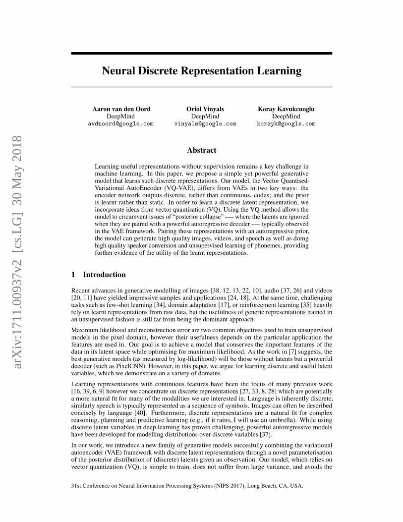
We define a latent embedding space e ∈ RK×D where K is the size of the discrete latent space (i.e.,a K-way categorical), and D is the dimensionality of each latent embedding vector ei. Note thatthere are K embedding vectors ei ∈ RD, i ∈ 1, 2, ...,K. As shown in Figure 1, the model takes aninput x, that is passed through an encoder producing output ze(x). The discrete latent variables zare then calculated by a nearest neighbour look-up using the shared embedding space e as shown inequation 1. The input to the decoder is the corresponding embedding vector ek as given in equation 2.One can see this forward computation pipeline as a regular autoencoder with a particular non-linearitythat maps the latents to 1-of-K embedding vectors. The complete set of parameters for the model areunion of parameters of the encoder, decoder, and the embedding space e. For sake of simplicity weuse a single random variable z to represent the discrete latent variables in this Section, however forspeech, image and videos we actually extract a 1D, 2D and 3D latent feature spaces respectively.

The posterior categorical distribution q(z|x) probabilities are defined as one-hot as follows:

q(z = k|x) ={1 for k = argminj‖ze(x)− ej‖2,0 otherwise

, (1)

where ze(x) is the output of the encoder network. We view this model as a VAE in which wecan bound log p(x) with the ELBO. Our proposal distribution q(z = k|x) is deterministic, and bydefining a simple uniform prior over z we obtain a KL divergence constant and equal to logK.

The representation ze(x) is passed through the discretisation bottleneck followed by mapping ontothe nearest element of embedding e as given in equations 1 and 2.

zq(x) = ek, where k = argminj‖ze(x)− ej‖2 (2)

3.2 Learning

Note that there is no real gradient defined for equation 2, however we approximate the gradientsimilar to the straight-through estimator [3] and just copy gradients from decoder input zq(x) toencoder output ze(x). One could also use the subgradient through the quantisation operation, but thissimple estimator worked well for the initial experiments in this paper.

3

Figure 1: Left: A figure describing the VQ-VAE. Right: Visualisation of the embedding space. Theoutput of the encoder z(x) is mapped to the nearest point e2. The gradient∇zL (in red) will push theencoder to change its output, which could alter the configuration in the next forward pass.

During forward computation the nearest embedding zq(x) (equation 2) is passed to the decoder, andduring the backwards pass the gradient ∇zL is passed unaltered to the encoder. Since the outputrepresentation of the encoder and the input to the decoder share the same D dimensional space,the gradients contain useful information for how the encoder has to change its output to lower thereconstruction loss.

As seen on Figure 1 (right), the gradient can push the encoder’s output to be discretised differently inthe next forward pass, because the assignment in equation 1 will be different.

Equation 3 specifies the overall loss function. It is has three components that are used to traindifferent parts of VQ-VAE. The first term is the reconstruction loss (or the data term) which optimizesthe decoder and the encoder (through the estimator explained above). Due to the straight-throughgradient estimation of mapping from ze(x) to zq(x), the embeddings ei receive no gradients fromthe reconstruction loss log p(z|zq(x)). Therefore, in order to learn the embedding space, we use oneof the simplest dictionary learning algorithms, Vector Quantisation (VQ). The VQ objective usesthe l2 error to move the embedding vectors ei towards the encoder outputs ze(x) as shown in thesecond term of equation 3. Because this loss term is only used for updating the dictionary, one canalternatively also update the dictionary items as function of moving averages of ze(x) (not used forthe experiments in this work). For more details see Appendix A.1.

Finally, since the volume of the embedding space is dimensionless, it can grow arbitrarily if theembeddings ei do not train as fast as the encoder parameters. To make sure the encoder commits toan embedding and its output does not grow, we add a commitment loss, the third term in equation 3.Thus, the total training objective becomes:

L = log p(x|zq(x)) + ‖sg[ze(x)]− e‖22 + β‖ze(x)− sg[e]‖22, (3)

where sg stands for the stopgradient operator that is defined as identity at forward computation timeand has zero partial derivatives, thus effectively constraining its operand to be a non-updated constant.The decoder optimises the first loss term only, the encoder optimises the first and the last loss terms,and the embeddings are optimised by the middle loss term. We found the resulting algorithm to bequite robust to β, as the results did not vary for values of β ranging from 0.1 to 2.0. We use β = 0.25in all our experiments, although in general this would depend on the scale of reconstruction loss.Since we assume a uniform prior for z, the KL term that usually appears in the ELBO is constantw.r.t. the encoder parameters and can thus be ignored for training.

In our experiments we define N discrete latents (e.g., we use a field of 32 x 32 latents for ImageNet,or 8 x 8 x 10 for CIFAR10). The resulting loss L is identical, except that we get an average over Nterms for k-means and commitment loss – one for each latent.

The log-likelihood of the complete model log p(x) can be evaluated as follows:

log p(x) = log∑k

p(x|zk)p(zk),

Because the decoder p(x|z) is trained with z = zq(x) from MAP-inference, the decoder should notallocate any probability mass to p(x|z) for z 6= zq(x) once it has fully converged. Thus, we can write

4

log p(x) ≈ log p(x|zq(x))p(zq(x)). We empirically evaluate this approximation in section 4. FromJensen’s inequality, we also can write log p(x) ≥ log p(x|zq(x))p(zq(x)).

3.3 Prior

The prior distribution over the discrete latents p(z) is a categorical distribution, and can be madeautoregressive by depending on other z in the feature map. Whilst training the VQ-VAE, the prior iskept constant and uniform. After training, we fit an autoregressive distribution over z, p(z), so thatwe can generate x via ancestral sampling. We use a PixelCNN over the discrete latents for images,and a WaveNet for raw audio. Training the prior and the VQ-VAE jointly, which could strengthen ourresults, is left as future research.

4 Experiments

4.1 Comparison with continuous variables

As a first experiment we compare VQ-VAE with normal VAEs (with continuous variables), as well asVIMCO [28] with independent Gaussian or categorical priors. We train these models using the samestandard VAE architecture on CIFAR10, while varying the latent capacity (number of continuous ordiscrete latent variables, as well as the dimensionality of the discrete space K). The encoder consistsof 2 strided convolutional layers with stride 2 and window size 4 × 4, followed by two residual3× 3 blocks (implemented as ReLU, 3x3 conv, ReLU, 1x1 conv), all having 256 hidden units. Thedecoder similarly has two residual 3× 3 blocks, followed by two transposed convolutions with stride2 and window size 4 × 4. We use the ADAM optimiser [21] with learning rate 2e-4 and evaluatethe performance after 250,000 steps with batch-size 128. For VIMCO we use 50 samples in themulti-sample training objective.

The VAE, VQ-VAE and VIMCO models obtain 4.51 bits/dim, 4.67 bits/dim and 5.14 respectively.All reported likelihoods are lower bounds. Our numbers for the continuous VAE are comparable tothose reported for a Deep convolutional VAE: 4.54 bits/dim [13] on this dataset.

Our model is the first among those using discrete latent variables which challenges the performanceof continuous VAEs. Thus, we get very good reconstructions like regular VAEs provide, with thecompressed representation that symbolic representations provide. A few interesting characteristics,implications and applications of the VQ-VAEs that we train is shown in the next subsections.

4.2 Images

Images contain a lot of redundant information as most of the pixels are correlated and noisy, thereforelearning models at the pixel level could be wasteful.

In this experiment we show that we can model x = 128× 128× 3 images by compressing them to az = 32× 32× 1 discrete space (with K=512) via a purely deconvolutional p(x|z). So a reduction of128×128×3×8

32×32×9 ≈ 42.6 in bits. We model images by learning a powerful prior (PixelCNN) over z. Thisallows to not only greatly speed up training and sampling, but also to use the PixelCNNs capacity tocapture the global structure instead of the low-level statistics of images.

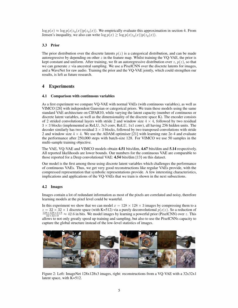
Figure 2: Left: ImageNet 128x128x3 images, right: reconstructions from a VQ-VAE with a 32x32x1latent space, with K=512.

5

Reconstructions from the 32x32x1 space with discrete latents are shown in Figure 2. Even consideringthat we greatly reduce the dimensionality with discrete encoding, the reconstructions look only slightlyblurrier than the originals. It would be possible to use a more perceptual loss function than MSE overpixels here (e.g., a GAN [12]), but we leave that as future work.

Next, we train a PixelCNN prior on the discretised 32x32x1 latent space. As we only have 1 channel(not 3 as with colours), we only have to use spatial masking in the PixelCNN. The capacity of thePixelCNN we used was similar to those used by the authors of the PixelCNN paper [38].

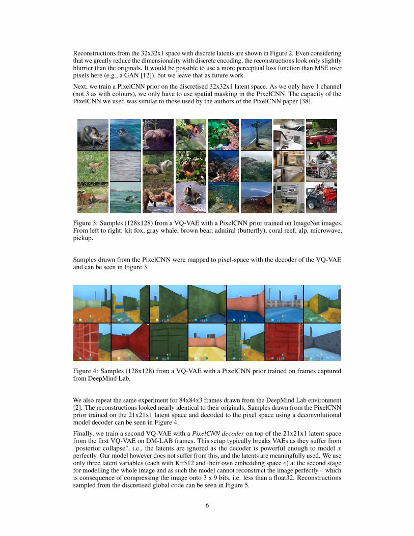
Figure 3: Samples (128x128) from a VQ-VAE with a PixelCNN prior trained on ImageNet images.From left to right: kit fox, gray whale, brown bear, admiral (butterfly), coral reef, alp, microwave,pickup.

Samples drawn from the PixelCNN were mapped to pixel-space with the decoder of the VQ-VAEand can be seen in Figure 3.

Figure 4: Samples (128x128) from a VQ-VAE with a PixelCNN prior trained on frames capturedfrom DeepMind Lab.

We also repeat the same experiment for 84x84x3 frames drawn from the DeepMind Lab environment[2]. The reconstructions looked nearly identical to their originals. Samples drawn from the PixelCNNprior trained on the 21x21x1 latent space and decoded to the pixel space using a deconvolutionalmodel decoder can be seen in Figure 4.

Finally, we train a second VQ-VAE with a PixelCNN decoder on top of the 21x21x1 latent spacefrom the first VQ-VAE on DM-LAB frames. This setup typically breaks VAEs as they suffer from"posterior collapse", i.e., the latents are ignored as the decoder is powerful enough to model xperfectly. Our model however does not suffer from this, and the latents are meaningfully used. We useonly three latent variables (each with K=512 and their own embedding space e) at the second stagefor modelling the whole image and as such the model cannot reconstruct the image perfectly – whichis consequence of compressing the image onto 3 x 9 bits, i.e. less than a float32. Reconstructionssampled from the discretised global code can be seen in Figure 5.

6

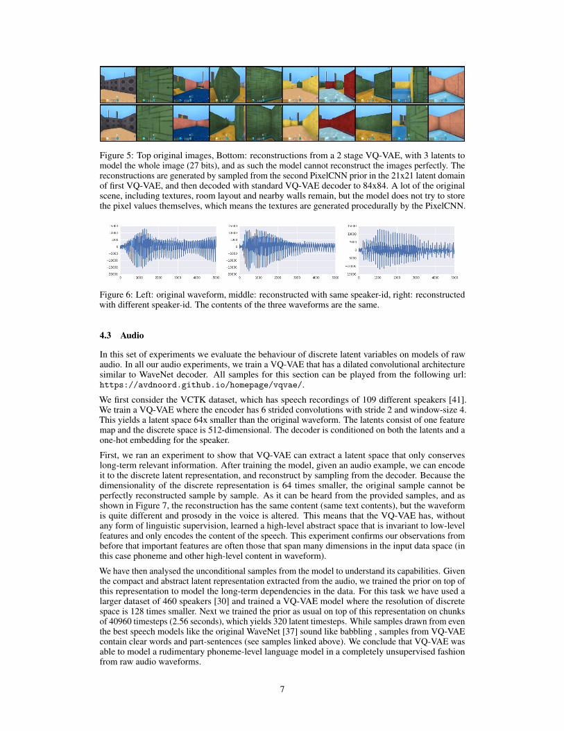
Figure 5: Top original images, Bottom: reconstructions from a 2 stage VQ-VAE, with 3 latents tomodel the whole image (27 bits), and as such the model cannot reconstruct the images perfectly. Thereconstructions are generated by sampled from the second PixelCNN prior in the 21x21 latent domainof first VQ-VAE, and then decoded with standard VQ-VAE decoder to 84x84. A lot of the originalscene, including textures, room layout and nearby walls remain, but the model does not try to storethe pixel values themselves, which means the textures are generated procedurally by the PixelCNN.

Figure 6: Left: original waveform, middle: reconstructed with same speaker-id, right: reconstructedwith different speaker-id. The contents of the three waveforms are the same.

4.3 Audio

In this set of experiments we evaluate the behaviour of discrete latent variables on models of rawaudio. In all our audio experiments, we train a VQ-VAE that has a dilated convolutional architecturesimilar to WaveNet decoder. All samples for this section can be played from the following url:https://avdnoord.github.io/homepage/vqvae/.

We first consider the VCTK dataset, which has speech recordings of 109 different speakers [41].We train a VQ-VAE where the encoder has 6 strided convolutions with stride 2 and window-size 4.This yields a latent space 64x smaller than the original waveform. The latents consist of one featuremap and the discrete space is 512-dimensional. The decoder is conditioned on both the latents and aone-hot embedding for the speaker.

First, we ran an experiment to show that VQ-VAE can extract a latent space that only conserveslong-term relevant information. After training the model, given an audio example, we can encodeit to the discrete latent representation, and reconstruct by sampling from the decoder. Because thedimensionality of the discrete representation is 64 times smaller, the original sample cannot beperfectly reconstructed sample by sample. As it can be heard from the provided samples, and asshown in Figure 7, the reconstruction has the same content (same text contents), but the waveformis quite different and prosody in the voice is altered. This means that the VQ-VAE has, withoutany form of linguistic supervision, learned a high-level abstract space that is invariant to low-levelfeatures and only encodes the content of the speech. This experiment confirms our observations frombefore that important features are often those that span many dimensions in the input data space (inthis case phoneme and other high-level content in waveform).

We have then analysed the unconditional samples from the model to understand its capabilities. Giventhe compact and abstract latent representation extracted from the audio, we trained the prior on top ofthis representation to model the long-term dependencies in the data. For this task we have used alarger dataset of 460 speakers [30] and trained a VQ-VAE model where the resolution of discretespace is 128 times smaller. Next we trained the prior as usual on top of this representation on chunksof 40960 timesteps (2.56 seconds), which yields 320 latent timesteps. While samples drawn from eventhe best speech models like the original WaveNet [37] sound like babbling , samples from VQ-VAEcontain clear words and part-sentences (see samples linked above). We conclude that VQ-VAE wasable to model a rudimentary phoneme-level language model in a completely unsupervised fashionfrom raw audio waveforms.

7

Next, we attempted the speaker conversion where the latents are extracted from one speaker and thenreconstructed through the decoder using a separate speaker id. As can be heard from the samples,the synthesised speech has the same content as the original sample, but with the voice from thesecond speaker. This experiment again demonstrates that the encoded representation has factored outspeaker-specific information: the embeddings not only have the same meaning regardless of detailsin the waveform, but also across different voice-characteristics.

Finally, in an attempt to better understand the content of the discrete codes we have compared thelatents one-to-one with the ground-truth phoneme-sequence (which was not used any way to train theVQ-VAE). With a 128-dimensional discrete space that runs at 25 Hz (encoder downsampling factorof 640), we mapped every of the 128 possible latent values to one of the 41 possible phoneme values1

(by taking the conditionally most likely phoneme). The accuracy of this 41-way classification was49.3%, while a random latent space would result in an accuracy of 7.2% (prior most likely phoneme).It is clear that these discrete latent codes obtained in a fully unsupervised way are high-level speechdescriptors that are closely related to phonemes.

4.4 Video

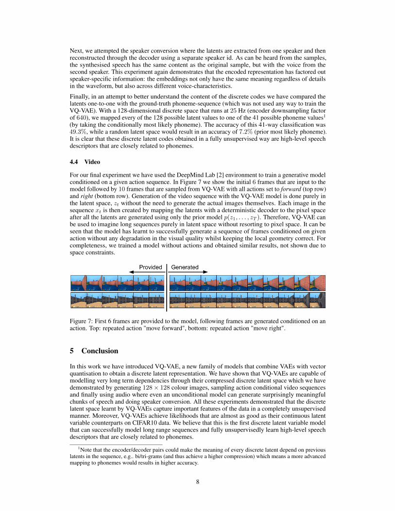
For our final experiment we have used the DeepMind Lab [2] environment to train a generative modelconditioned on a given action sequence. In Figure 7 we show the initial 6 frames that are input to themodel followed by 10 frames that are sampled from VQ-VAE with all actions set to forward (top row)and right (bottom row). Generation of the video sequence with the VQ-VAE model is done purely inthe latent space, zt without the need to generate the actual images themselves. Each image in thesequence xt is then created by mapping the latents with a deterministic decoder to the pixel spaceafter all the latents are generated using only the prior model p(z1, . . . , zT ). Therefore, VQ-VAE canbe used to imagine long sequences purely in latent space without resorting to pixel space. It can beseen that the model has learnt to successfully generate a sequence of frames conditioned on givenaction without any degradation in the visual quality whilst keeping the local geometry correct. Forcompleteness, we trained a model without actions and obtained similar results, not shown due tospace constraints.

Figure 7: First 6 frames are provided to the model, following frames are generated conditioned on anaction. Top: repeated action "move forward", bottom: repeated action "move right".

5 Conclusion

In this work we have introduced VQ-VAE, a new family of models that combine VAEs with vectorquantisation to obtain a discrete latent representation. We have shown that VQ-VAEs are capable ofmodelling very long term dependencies through their compressed discrete latent space which we havedemonstrated by generating 128× 128 colour images, sampling action conditional video sequencesand finally using audio where even an unconditional model can generate surprisingly meaningfulchunks of speech and doing speaker conversion. All these experiments demonstrated that the discretelatent space learnt by VQ-VAEs capture important features of the data in a completely unsupervisedmanner. Moreover, VQ-VAEs achieve likelihoods that are almost as good as their continuous latentvariable counterparts on CIFAR10 data. We believe that this is the first discrete latent variable modelthat can successfully model long range sequences and fully unsupervisedly learn high-level speechdescriptors that are closely related to phonemes.

1Note that the encoder/decoder pairs could make the meaning of every discrete latent depend on previouslatents in the sequence, e.g.. bi/tri-grams (and thus achieve a higher compression) which means a more advancedmapping to phonemes would results in higher accuracy.

8

References[1] Eirikur Agustsson, Fabian Mentzer, Michael Tschannen, Lukas Cavigelli, Radu Timofte, Luca Benini, and

Luc Van Gool. Soft-to-hard vector quantization for end-to-end learned compression of images and neuralnetworks. arXiv preprint arXiv:1704.00648, 2017.

[2] Charles Beattie, Joel Z Leibo, Denis Teplyashin, Tom Ward, Marcus Wainwright, Heinrich Küttler, AndrewLefrancq, Simon Green, Víctor Valdés, Amir Sadik, et al. Deepmind lab. arXiv preprint arXiv:1612.03801,2016.

[3] Yoshua Bengio, Nicholas Léonard, and Aaron Courville. Estimating or propagating gradients throughstochastic neurons for conditional computation. arXiv preprint arXiv:1308.3432, 2013.

[4] Samuel R Bowman, Luke Vilnis, Oriol Vinyals, Andrew M Dai, Rafal Jozefowicz, and Samy Bengio.Generating sentences from a continuous space. arXiv preprint arXiv:1511.06349, 2015.

[5] Yuri Burda, Roger Grosse, and Ruslan Salakhutdinov. Importance weighted autoencoders. arXiv preprintarXiv:1509.00519, 2015.

[6] Xi Chen, Yan Duan, Rein Houthooft, John Schulman, Ilya Sutskever, and Pieter Abbeel. Infogan:Interpretable representation learning by information maximizing generative adversarial nets. CoRR,abs/1606.03657, 2016.

[7] Xi Chen, Diederik P Kingma, Tim Salimans, Yan Duan, Prafulla Dhariwal, John Schulman, Ilya Sutskever,and Pieter Abbeel. Variational lossy autoencoder. arXiv preprint arXiv:1611.02731, 2016.

[8] Aaron Courville, James Bergstra, and Yoshua Bengio. A spike and slab restricted boltzmann machine. InProceedings of the Fourteenth International Conference on Artificial Intelligence and Statistics, pages233–241, 2011.

[9] Emily Denton, Sam Gross, and Rob Fergus. Semi-supervised learning with context-conditional generativeadversarial networks. arXiv preprint arXiv:1611.06430, 2016.

[10] Laurent Dinh, Jascha Sohl-Dickstein, and Samy Bengio. Density estimation using real nvp. arXiv preprintarXiv:1605.08803, 2016.

[11] Chelsea Finn, Ian Goodfellow, and Sergey Levine. Unsupervised learning for physical interaction throughvideo prediction. In Advances in Neural Information Processing Systems, pages 64–72, 2016.

[12] Ian Goodfellow, Jean Pouget-Abadie, Mehdi Mirza, Bing Xu, David Warde-Farley, Sherjil Ozair, AaronCourville, and Yoshua Bengio. Generative adversarial nets. In Advances in neural information processingsystems, pages 2672–2680, 2014.

[13] Karol Gregor, Frederic Besse, Danilo Jimenez Rezende, Ivo Danihelka, and Daan Wierstra. Towardsconceptual compression. In Advances In Neural Information Processing Systems, pages 3549–3557, 2016.

[14] Karol Gregor, Ivo Danihelka, Andriy Mnih, Charles Blundell, and Daan Wierstra. Deep autoregressivenetworks. arXiv preprint arXiv:1310.8499, 2013.

[15] Ishaan Gulrajani, Kundan Kumar, Faruk Ahmed, Adrien Ali Taiga, Francesco Visin, David Vázquez, andAaron C. Courville. Pixelvae: A latent variable model for natural images. CoRR, abs/1611.05013, 2016.

[16] Geoffrey E Hinton and Ruslan R Salakhutdinov. Reducing the dimensionality of data with neural networks.science, 313(5786):504–507, 2006.

[17] Judy Hoffman, Erik Rodner, Jeff Donahue, Trevor Darrell, and Kate Saenko. Efficient learning ofdomain-invariant image representations. arXiv preprint arXiv:1301.3224, 2013.

[18] Phillip Isola, Jun-Yan Zhu, Tinghui Zhou, and Alexei A Efros. Image-to-image translation with conditionaladversarial networks. arXiv preprint arXiv:1611.07004, 2016.

[19] Eric Jang, Shixiang Gu, and Ben Poole. Categorical reparameterization with gumbel-softmax. arXivpreprint arXiv:1611.01144, 2016.

[20] Nal Kalchbrenner, Aaron van den Oord, Karen Simonyan, Ivo Danihelka, Oriol Vinyals, Alex Graves, andKoray Kavukcuoglu. Video pixel networks. arXiv preprint arXiv:1610.00527, 2016.

[21] Diederik Kingma and Jimmy Ba. Adam: A method for stochastic optimization. arXiv preprintarXiv:1412.6980, 2014.

[22] Diederik P Kingma, Tim Salimans, Rafal Jozefowicz, Xi Chen, Ilya Sutskever, and Max Welling. Improvedvariational inference with inverse autoregressive flow. NIPS 2016, 2016.

[23] Diederik P Kingma and Max Welling. Auto-encoding variational bayes. arXiv preprint arXiv:1312.6114,2013.

[24] Christian Ledig, Lucas Theis, Ferenc Huszár, Jose Caballero, Andrew Cunningham, Alejandro Acosta,Andrew Aitken, Alykhan Tejani, Johannes Totz, Zehan Wang, et al. Photo-realistic single image super-resolution using a generative adversarial network. arXiv preprint arXiv:1609.04802, 2016.

9

[25] Chris J Maddison, Andriy Mnih, and Yee Whye Teh. The concrete distribution: A continuous relaxation ofdiscrete random variables. arXiv preprint arXiv:1611.00712, 2016.

[26] Soroush Mehri, Kundan Kumar, Ishaan Gulrajani, Rithesh Kumar, Shubham Jain, Jose Sotelo, AaronCourville, and Yoshua Bengio. Samplernn: An unconditional end-to-end neural audio generation model.arXiv preprint arXiv:1612.07837, 2016.

[27] Andriy Mnih and Karol Gregor. Neural variational inference and learning in belief networks. arXivpreprint arXiv:1402.0030, 2014.

[28] Andriy Mnih and Danilo Jimenez Rezende. Variational inference for monte carlo objectives. CoRR,abs/1602.06725, 2016.

[29] Aaron van den Oord, Nal Kalchbrenner, and Koray Kavukcuoglu. Pixel recurrent neural networks. arXivpreprint arXiv:1601.06759, 2016.

[30] Vassil Panayotov, Guoguo Chen, Daniel Povey, and Sanjeev Khudanpur. Librispeech: an asr corpusbased on public domain audio books. In Acoustics, Speech and Signal Processing (ICASSP), 2015 IEEEInternational Conference on, pages 5206–5210. IEEE, 2015.

[31] Danilo Jimenez Rezende and Shakir Mohamed. Variational inference with normalizing flows. arXivpreprint arXiv:1505.05770, 2015.

[32] Danilo Jimenez Rezende, Shakir Mohamed, and Daan Wierstra. Stochastic backpropagation and approxi-mate inference in deep generative models. arXiv preprint arXiv:1401.4082, 2014.

[33] Ruslan Salakhutdinov and Geoffrey Hinton. Deep boltzmann machines. In Artificial Intelligence andStatistics, pages 448–455, 2009.

[34] Adam Santoro, Sergey Bartunov, Matthew Botvinick, Daan Wierstra, and Timothy Lillicrap. One-shotlearning with memory-augmented neural networks. arXiv preprint arXiv:1605.06065, 2016.

[35] Richard S Sutton and Andrew G Barto. Reinforcement learning: An introduction, volume 1. MIT pressCambridge, 1998.

[36] Lucas Theis, Wenzhe Shi, Andrew Cunningham, and Ferenc Huszár. Lossy image compression withcompressive autoencoders. arXiv preprint arXiv:1703.00395, 2017.

[37] Aäron van den Oord, Sander Dieleman, Heiga Zen, Karen Simonyan, Oriol Vinyals, Alex Graves, NalKalchbrenner, Andrew Senior, and Koray Kavukcuoglu. Wavenet: A generative model for raw audio.CoRR abs/1609.03499, 2016.

[38] Aaron van den Oord, Nal Kalchbrenner, Lasse Espeholt, Oriol Vinyals, Alex Graves, et al. Conditionalimage generation with pixelcnn decoders. In Advances in Neural Information Processing Systems, pages4790–4798, 2016.

[39] Pascal Vincent, Hugo Larochelle, Isabelle Lajoie, Yoshua Bengio, and Pierre-Antoine Manzagol. Stackeddenoising autoencoders: Learning useful representations in a deep network with a local denoising criterion.Journal of Machine Learning Research, 11(Dec):3371–3408, 2010.

[40] Oriol Vinyals, Alexander Toshev, Samy Bengio, and Dumitru Erhan. Show and tell: A neural imagecaption generator. In Proceedings of the IEEE Conference on Computer Vision and Pattern Recognition,pages 3156–3164, 2015.

[41] Junichi Yamagishi. English multi-speaker corpus for cstr voice cloning toolkit. URL http://homepages. inf.ed. ac. uk/jyamagis/page3/page58/page58. html, 2012.

[42] Zichao Yang, Zhiting Hu, Ruslan Salakhutdinov, and Taylor Berg-Kirkpatrick. Improved variationalautoencoders for text modeling using dilated convolutions. CoRR, abs/1702.08139, 2017.

10

A Appendix

A.1 VQ-VAE dictionary updates with Exponential Moving Averages

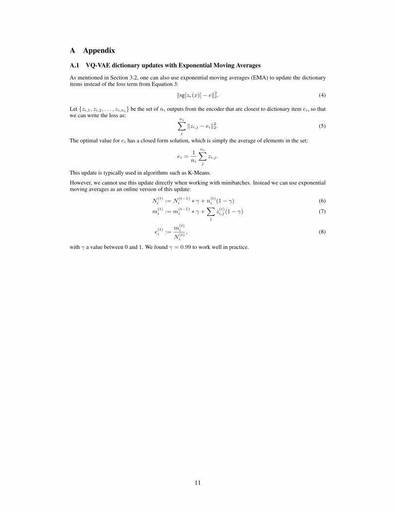
As mentioned in Section 3.2, one can also use exponential moving averages (EMA) to update the dictionaryitems instead of the loss term from Equation 3:

‖sg[ze(x)]− e‖22. (4)

Let {zi,1, zi,2, . . . , zi,ni} be the set of ni outputs from the encoder that are closest to dictionary item ei, so thatwe can write the loss as:

ni∑j

‖zi,j − ei‖22. (5)

The optimal value for ei has a closed form solution, which is simply the average of elements in the set:

ei =1

ni

ni∑j

zi,j .

This update is typically used in algorithms such as K-Means.

However, we cannot use this update directly when working with minibatches. Instead we can use exponentialmoving averages as an online version of this update:

N(t)i := N

(t−1)i ∗ γ + n

(t)i (1− γ) (6)

m(t)i := m

(t−1)i ∗ γ +

∑j

z(t)i,j (1− γ) (7)

e(t)i :=

m(t)i

N(t)i

, (8)

with γ a value between 0 and 1. We found γ = 0.99 to work well in practice.

11