deep learning for audio - university of...

Deep Learning for AudioYUCHEN FAN, MATT POTOK, CHRISTOPHER SHROBA

MotivationText-to-Speech

◦ Accessibility features for people with little to no vision, or people in situations where they cannot look at a screen or other textual source

◦ Natural language interfaces for a more fluid and natural way to interact with computers

◦ Voice Assistants (Siri, etc.), GPS, Screen Readers, Automated telephony systems

Automatic Speech Recognition◦ Again, natural language interfaces

◦ Alternative input medium for accessibility purposes

◦ Voice Assistants (Siri, etc.), Automated telephony systems, Hands-free phone control in the car

Music Generation◦ Mostly for fun

◦ Possible applications in music production software

OutlineAutomatic Speech Recognition (ASR)

◦ Deep models with HMMs

◦ Connectionist Temporal Classification (CTC)

◦ Attention based models

Text to Speech (TTS)◦ WaveNet

◦ DeepVoice

◦ Tacotron

Bonus: Music Generation

Automatic Speech Recognition (ASR)

OutlineHistory of Automatic Speech Recognition

Hidden Markov Model (HMM) based Automatic Speech Recognition◦ Gaussian mixture models with HMMs


End-to-End Deep Models based Automatic Speech Recognition◦ Connectionist Temporal Classification (CTC)


History of Automatic Speech RecognitionEarly 1970s: Dynamic Time Warping (DTW) to handle time variability

◦ Distance measure for spectral variability

http://publications.csail.mit.edu/abstracts/abstracts06/malex/seg_dtw.jpg

History of Automatic Speech RecognitionMid-Late 1970s: Hidden Markov Models (HMMs) – statistical models of spectral variations, for discrete speech.

Mid 1980s: HMMs become the dominant technique for all ASR

01

23

45

(kH

z)

a i silsil

http://hts.sp.nitech.ac.jp/archives/2.3/HTS_Slides.zip

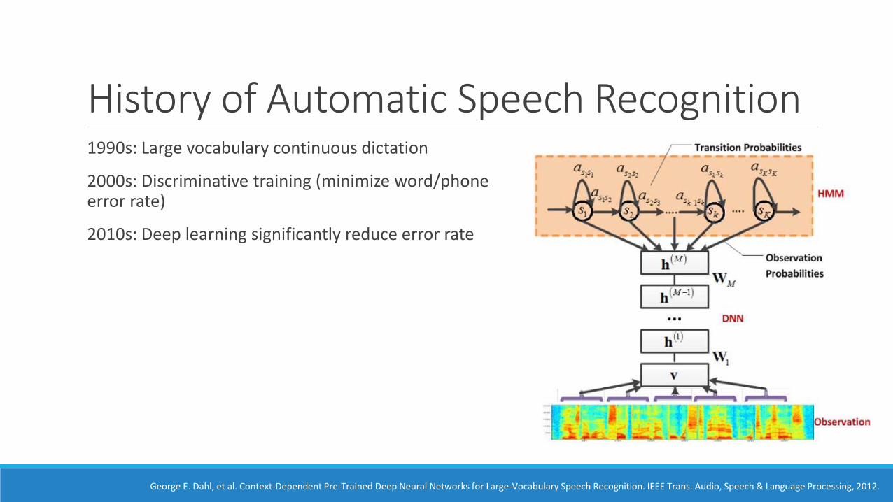
History of Automatic Speech Recognition1990s: Large vocabulary continuous dictation

2000s: Discriminative training (minimize word/phone error rate)

2010s: Deep learning significantly reduce error rate

George E. Dahl, et al. Context-Dependent Pre-Trained Deep Neural Networks for Large-Vocabulary Speech Recognition. IEEE Trans. Audio, Speech & Language Processing, 2012.

Aim of Automatic Speech RecognitionFind the most likely sentence (word sequence) 𝑾, which transcribes the speech audio 𝑨:

𝑾 = argmax𝑾

𝑃 𝑾 𝑨 = argmax𝑾

𝑃 𝑨 𝑾 𝑃(𝑾)

◦ Acoustic model 𝑃 𝑨 𝑾

◦ Language model 𝑃(𝑾)

Training: find parameters for acoustic and language model separately◦ Speech Corpus: speech waveform and human-annotated transcriptions

◦ Language model: with extra data (prefer daily expressions corpus for spontaneous speech)

Language modelLanguage model is a probabilistic model used to

◦ Guide the search algorithm (predict next word given history)

◦ Disambiguate between phrases which are acoustically similar◦ Great wine vs Grey twine

It assigns probability to a sequence of tokens to be finally recognized

N-gram model 𝑃 𝑤𝑁 𝑤1, 𝑤2, ⋯ , 𝑤𝑁−1

Recurrent neural network

http://torch.ch/blog/2016/07/25/nce.html

Recurrent neural network based Language model

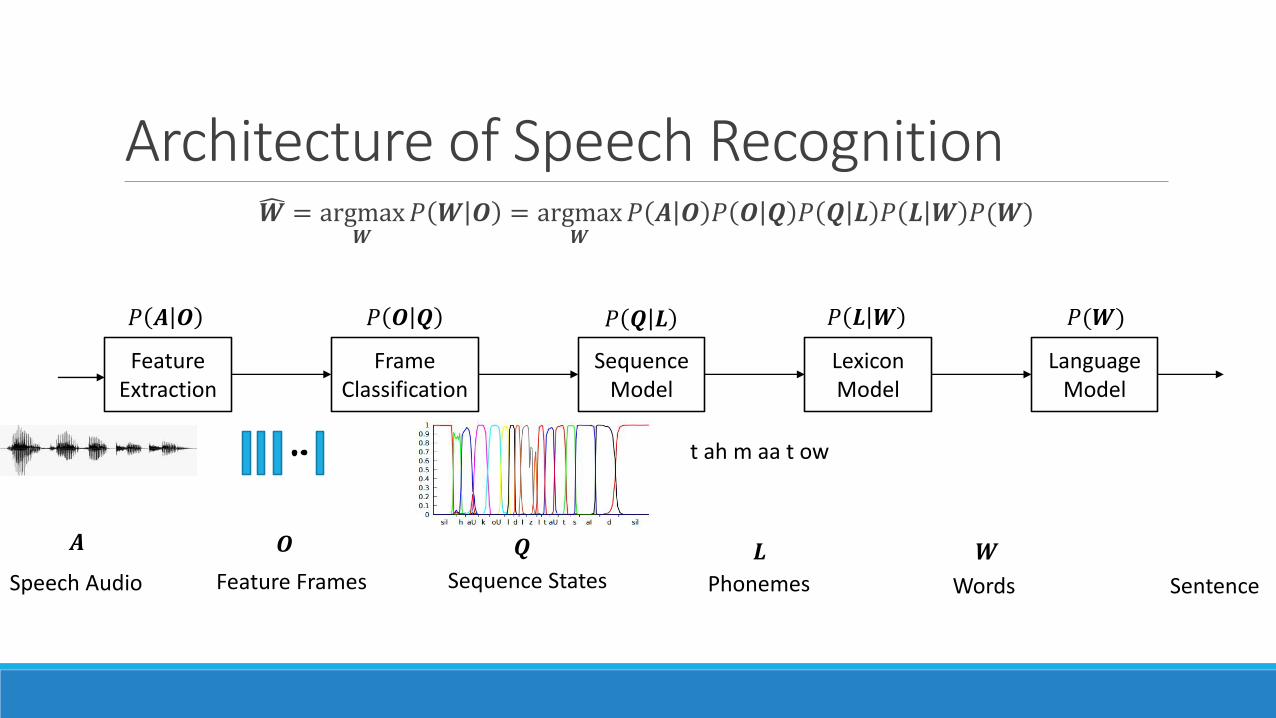
Architecture of Speech Recognition𝑾 = argmax

𝑾𝑃 𝑾 𝑶 = argmax

𝑾𝑃 𝑨 𝑶 𝑃 𝑶 𝑸 𝑃 𝑸 𝑳 𝑃 𝑳 𝑾 𝑃(𝑾)

𝑨

FeatureExtraction

FrameClassification

SequenceModel

LexiconModel

LanguageModel

Speech Audio Feature Frames

𝑶

𝑃 𝑨 𝑶 𝑃 𝑶 𝑸 𝑃 𝑸 𝑳

𝑸

Sequence States

t ah m aa t ow

𝑃 𝑳 𝑾 𝑃(𝑾)

𝑳

Phonemes

𝑾

Words Sentence

Decoding in Speech RecognitionFind most likely word sequence of audio input

Without language models With language models

https://www.inf.ed.ac.uk/teaching/courses/asr/2011-12/asr-search-nup4.pdf




𝑨

FeatureExtraction

FrameClassification

SequenceModel

LexiconModel

LanguageModel


𝑶


𝑸

Sequence States

t ah m aa t ow


𝑳

Phonemes

𝑾

Words Sentence

deterministic




𝑨

FeatureExtraction

FrameClassification

SequenceModel

LexiconModel

LanguageModel


𝑶


𝑸

Sequence States

t ah m aa t ow


𝑳

Phonemes

𝑾

Words Sentence

Feature ExtractionRaw waveforms are transformed into a sequence of feature vectors using signal processing approaches

Time domain to frequency domain

Feature extraction is a deterministic process𝑃 𝑨 𝑶 = 𝛿(𝐴, መ𝐴(𝑂))

Reduce information rate but keep useful information◦ Remove noise and other irrelevant information

Extracted in 25ms windows and shifted with 10ms

Still useful for deep models

http://www2.cmpe.boun.edu.tr/courses/cmpe362/spring2014/files/projects/MFCC%20Feature%20Extraction.pdf

Different Level Features

http://music.ece.drexel.edu/research/voiceID/researchday2007

Better for shallow models

Better for deep models




𝑨

FeatureExtraction

FrameClassification

SequenceModel

LexiconModel

LanguageModel


𝑶


𝑸

Sequence States

t ah m aa t ow


𝑳

Phonemes

𝑾

Words Sentence

Lexical modelLexical modelling forms the bridge between the acoustic and language models

Prior knowledge of language

Mapping between words and the acoustic units (phoneme is most common)Deterministic Probabilistic

Word Pronunciation

TOMATOt ah m aa t ow

t ah m ey t ow

COVERAGEk ah v er ah jh

k ah v r ah jh

Word Pronunciation Probability

TOMATOt ah m aa t ow 0.45

t ah m ey t ow 0.55

COVERAGEk ah v er ah jh 0.65

k ah v r ah jh 0.35

GMM-HMM in Speech RecognitionGMMs: Gaussian Mixture Models

HMMs: Hidden Markov Models

𝑨

FeatureExtraction

FrameClassification

SequenceModel

LexiconModel

LanguageModel


𝑶

GMMs HMMs

𝑸

Sequence States

t ah m aa t ow

𝑳

Phonemes

𝑾

Words Sentence

Hidden Markov ModelsThe Markov chain whose state sequence is unknown

11a 22a 33a

12a 23a

)(1 tb o )(2 tb o )(3 tb o

1o 2o 3o 4o 5oTo ・・

1 2 3

1 1 1 1 2 2 3 3

o

q

Observation

sequence

State sequence

ija

)( tqb o

: State transition probability

: Output probability


Context Dependent ModelWe were away with William in Sea World

Realization of w varies but similar patterns occur in the similar context

Context Dependent ModelIn English

#Monophone : 46

#Biphone: 2116

#Triphone: 97336

s a cl p a r i w a k a r a n a iPhoneme

sequence

s-a-cl p-a-r n-a-i

Context-dependent HMMs


Decision Tree-based State ClusteringEach state separated automatically by the optimum question

k-a+b

t-a+h

…

…

…

yes

yes

yesyes

yes no

no

no

no

no

R=silence?

L=“gy”?

L=voice?

L=“w”?

R=silence?

C=unvoice?C=vowel?R=silence?R=“cl”?L=“gy”?L=voice?… Sharing the parameter of HMMs in same leaf node

s-i+n




𝑨

FeatureExtraction

FrameClassification

SequenceModel

LexiconModel

LanguageModel


𝑶

GMMs HMMs

𝑸

Sequence States

t ah m aa t ow

𝑳

Phonemes

𝑾

Words Sentence

Gaussian Mixture ModelsOutput probability is modeled by Gaussian mixture models

𝑏𝒒 𝒐𝑡 = 𝑏 𝒐𝑡 𝒒𝑡

=

𝑚=1

𝑀

𝑤𝒒𝑡,𝑚𝑁 𝒐𝑡 𝝁𝑚, 𝚺𝑚2,1w 2,2w

2,3w2

2

nR

)(12 xN )(22 xN )(32 xN

Mw ,1 Mw ,2 Mw ,3Mn

M R

)(1 xMN )(2 xMN )(3 xMN

1 2 3

1,1w 1,2w1,3w

1

1

nR

)(11 xN )(21 xN )(31 xN




𝑨

FeatureExtraction

FrameClassification

SequenceModel

LexiconModel

LanguageModel


𝑶

GMMs HMMs

𝑸

Sequence States

t ah m aa t ow

𝑳

Phonemes

𝑾

Words Sentence

DNN-HMM in Speech RecognitionDNN: Deep Neural Networks


𝑨

FeatureExtraction

FrameClassification

SequenceModel

LexiconModel

LanguageModel


𝑶

DNNs HMMs

𝑸

Sequence States

t ah m aa t ow

𝑳

Phonemes

𝑾

Words Sentence

Ingredients for Deep LearningAcoustic features

◦ Frequency domain features extracted from waveform

◦ 10ms interval between frames

◦ ~40 dimensions for each frame

State alignments◦ Tied-state of context-dependent HMMs

◦ Mapping between acoustic features and states



𝑨

FeatureExtraction

FrameClassification

SequenceModel

LexiconModel

LanguageModel


𝑶

DNNs HMMs

𝑸

Sequence States

t ah m aa t ow

𝑳

Phonemes

𝑾

Words Sentence

Deep Models in HMM-based ASRClassify acoustic features for state labels

Take softmax output as a posterior 𝑃 𝑠𝑡𝑎𝑡𝑒 𝒐𝑡 = 𝑃 𝒒𝑡 𝒐𝑡

Work as output probability in HMM

𝑏𝒒 𝒐𝑡 = 𝑏 𝒐𝑡 𝒒𝑡 =𝑃 𝒒𝑡 𝒐𝑡 𝑃(𝒐𝑡)

𝑃(𝒒𝑡)

where 𝑃(𝒒𝑡) is the prior probability for states

Fully Connected NetworksFeatures including 2 X 5 neighboring frames

◦ 1D convolution with kernel size 11

Classify 9,304 tied states

7 hidden layers X 2048 units with sigmoid activation

G. Hinton, et al. Deep Neural Networks for Acoustic Modeling in Speech Recognition. Signal Processing Magazine (2012).

Fully Connected NetworksPre-training

◦ Unsupervised: stacked restricted Boltzmann machine (RBM)

◦ Supervised: iteratively adding layers from shallow model

Training◦ Maximum cross entropy for frames

Fine-tuning◦ Maximum mutual information for sequences


Fully Connected NetworksComparison on different large datasets


DNN-HMM vs. GMM-HMMDeep models are more powerful

◦ GMM assumes data is generated from single component of mixture model

◦ GMM with diagonal variance matrix ignores correlation between dimensions

Deep models take data more efficiently◦ GMM consists with many components and each learns from a small fraction of data

Deep models can be further improved by recent advances in deep learning

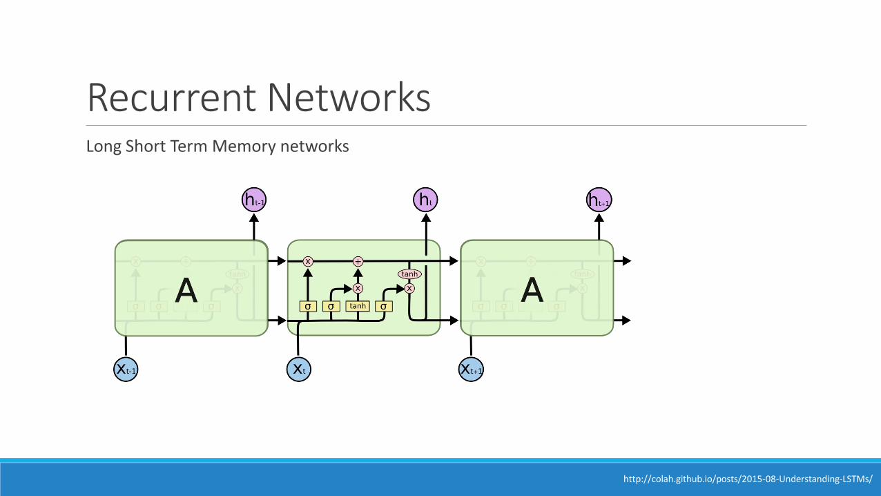
Recurrent NetworksLong Short Term Memory networks

http://colah.github.io/posts/2015-08-Understanding-LSTMs/

Recurrent Networks

H. Sak, A. Senior, and F. Beaufays. Long Short-Term Memory Recurrent Neural Network Architectures for Large Scale Acoustic Modeling. arXiv preprint arXiv:1402.1128v1 (2014).

Very Deep Networks

W. Xiong, et al. Achieving Human Parity in Conversational Speech Recognition. arXiv preprint arXiv:1610.05256 (2016).

LACE

Very Deep NetworksSpeaker adaptive training

◦ Addition speaker id embedded vector as input

Language model with LSTM

System combination◦ Greedy-searched weight to combine multiple model system

Reuslts on the test set: CH and SWB Exceed human accuracy

Word error rates CH SWB

ResNet 14.8 8.6

VGG 15.7 9.1

LACE 15.0 8.4

Limitations of DNN-HMMMarkov models only depend one previous states

History is discretely represented by 10k states

Decoding is slow to keep all 10k state in dynamic programing

Decoding with dynamic programing



𝑨

FeatureExtraction

FrameClassification

SequenceModel

LexiconModel

LanguageModel


𝑶

DNNs HMMs

𝑸

Sequence States

t ah m aa t ow

𝑳

Phonemes

𝑾

Words Sentence

End-to-End Deep Models based Automatic Speech RecognitionConnectionist Temporal Classification (CTC) based models

◦ LSTM CTC models

◦ Deep speech 2

Attention based models

CTC in Speech RecognitionRNN: Recurrent Neural Networks

CTC: Connectionist Temporal Classification

𝑨

FeatureExtraction

FrameClassification

SequenceModel

LexiconModel

LanguageModel


𝑶

RNNs CTC

𝑸

Sequence States

t ah m aa t ow

𝑳

Phonemes

𝑾

Words Sentence

Connectionist Temporal Classification (CTC)

https://gab41.lab41.org/speech-recognition-you-down-with-ctc-8d3b558943f0, ftp://ftp.idsia.ch/pub/juergen/icml2006.pdf

Method for labeling unsegmented data sequences◦ Raw waveforms and text transcription

Differentiable objective function◦ Gradient based training

◦ 𝑂𝑀𝐿 𝑆,𝒩𝑤 = −σ 𝑥,𝑧 ∈𝑆 ln 𝑝 𝑧 𝑥

Used in various ASR and TTS architectures◦ DeepSpeech (ASR)

◦ DeepVoice(TTS)

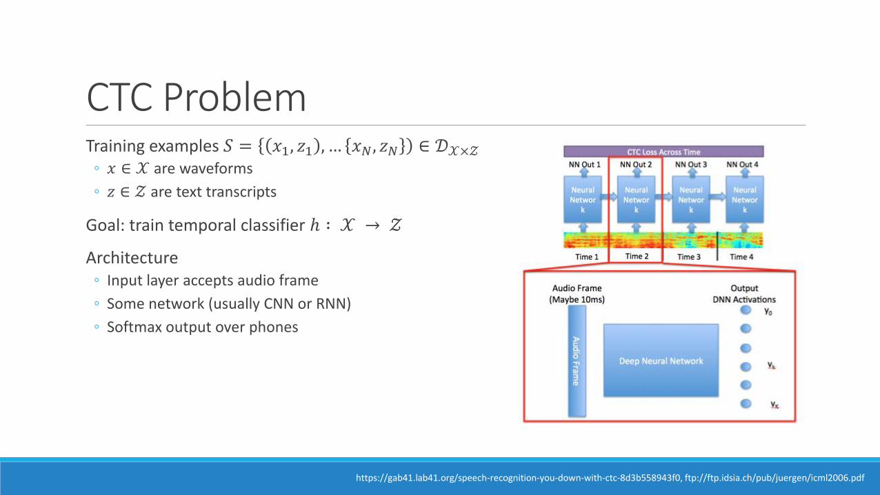
CTC ProblemTraining examples 𝑆 = 𝑥1, 𝑧1 , … 𝑥𝑁, 𝑧𝑁 ∈ 𝒟𝒳×𝒵

◦ 𝑥 ∈ 𝒳 are waveforms

◦ 𝑧 ∈ 𝒵 are text transcripts

Goal: train temporal classifier ℎ ∶ 𝒳 → 𝒵

Architecture◦ Input layer accepts audio frame

◦ Some network (usually CNN or RNN)

◦ Softmax output over phones


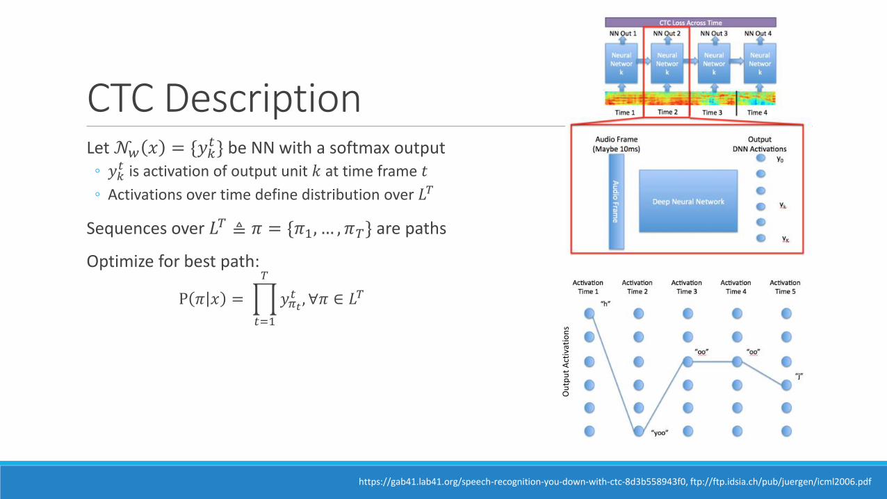
CTC DescriptionLet 𝒩𝑤 𝑥 = {𝑦𝑘

𝑡} be NN with a softmax output◦ 𝑦𝑘

𝑡 is activation of output unit 𝑘 at time frame 𝑡

◦ Activations over time define distribution over 𝐿𝑇

Sequences over 𝐿𝑇 ≜ 𝜋 = {𝜋1, … , 𝜋𝑇} are paths

Optimize for best path:

P 𝜋 𝑥 = ෑ

𝑡=1

𝑇

𝑦𝜋𝑡𝑡 , ∀𝜋 ∈ 𝐿𝑇

Ou

tpu

t A

ctiv

atio

ns


CTC ObjectivePaths are not equivalent to the label, 𝜋 ≠ 𝑙

Optimize for best label:

𝑃 𝑙 𝑥 =

𝜋

𝑃 𝑙 𝜋 𝑃 𝜋 𝑥

Solve objective above with dynamic time warping◦ Forward-backward algorithm

◦ Forward variables 𝛼

◦ Backward variables 𝛽

𝑃 𝑙 𝑥 =

𝑠=1

|𝑙|𝛼𝑡 𝑠 𝛽𝑡 𝑠

𝑦𝑙𝑠𝑡

◦ Maps and searches only paths that correspond to target label

𝑙 = {𝑎} 𝑙 = {𝑏𝑒𝑒}

https://github.com/yiwangbaidu/notes/blob/master/CTC/CTC.pdf, ftp://ftp.idsia.ch/pub/juergen/icml2006.pdf

CTC Objective and GradientObjective function:

𝑂𝑀𝐿 𝑆,𝒩𝑤 = −

𝑥,𝑧 ∈𝑆

ln 𝑝 𝑧 𝑥

Gradient:𝜕𝑂𝑀𝐿 { 𝑥, 𝑧 },𝒩𝑤

𝜕𝑢𝑘𝑡 = 𝑦𝑘

𝑡 −1

𝑦𝑘𝑡𝑍𝑡

𝑠∈𝑙𝑎𝑏 𝑧,𝑘

ො𝛼𝑡 𝑠 መ𝛽𝑡 𝑠

where 𝑍𝑡 ≜

𝑠=1

|𝑙′|𝛼𝑡 𝑠 𝛽𝑡 𝑠

𝑦𝑙𝑠′𝑡

ftp://ftp.idsia.ch/pub/juergen/icml2006.pdf

LSTM CTC ModelsWord error rate compared with HMM based models

Bi-direction LSTM is more essential for CTC

Context Error Rate (%)

LSTM-HMM Uni 8.9

Bi 9.1

LSTM-CTC Uni 9.4

Bi 8.5

Sak, Haşim, et al. "Learning acoustic frame labeling for speech recognition with recurrent neural networks." ICASSP, 2015.

CTC vs HMMOutput probability of LSTM

HMM CTC

CTC embeds history in continuous hidden space, more capable than HMM

CTC has spiky predictions, more discriminable between states than HMM

CTC with less states (40) is significantly faster for decoding than HMM (10k states)

Sak, Haşim, et al. "Learning acoustic frame labeling for speech recognition with recurrent neural networks." ICASSP, 2015.

Deep Speech 23 layers of 2D-invariant convolution

7 layers of bidirectional simple recurrence

100M parameters

Word error rates

Test set Deep speech 2 Human

WSJ eval’92 3.60 5.03

WSJ eval’93 4.98 8.08

LibriSpeech test-clean

5.33 5.83

LibriSpeech test-other

13.25 12.69

Amodei, Dario, et al. "Deep speech 2: End-to-end speech recognition in english and mandarin." arXiv preprint arXiv:1512.02595 (2015).

CTC in Speech RecognitionRNN: Recurrent Neural Networks

CTC: Connectionist Temporal Classification

𝑨

FeatureExtraction

FrameClassification

SequenceModel

LexiconModel

LanguageModel


𝑶

RNNs CTC

𝑸

Sequence States

t ah m aa t ow

𝑳

Phonemes

𝑾

Words Sentence

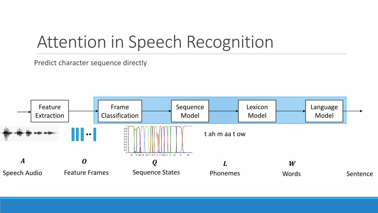
Attention in Speech RecognitionPredict character sequence directly

𝑨

FeatureExtraction

FrameClassification

SequenceModel

LexiconModel

LanguageModel


𝑶 𝑸

Sequence States

t ah m aa t ow

𝑳

Phonemes

𝑾

Words Sentence

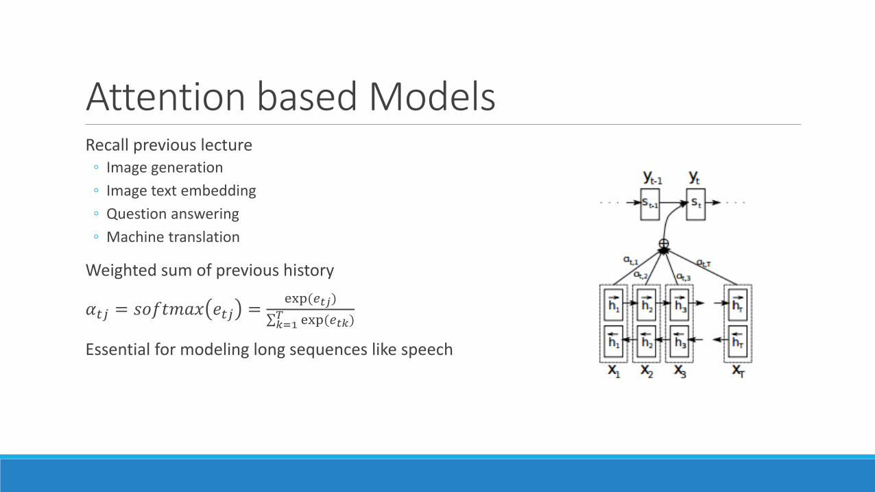
Attention based Models Recall previous lecture

◦ Image generation

◦ Image text embedding

◦ Question answering

◦ Machine translation

Weighted sum of previous history

𝛼𝑡𝑗 = 𝑠𝑜𝑓𝑡𝑚𝑎𝑥 𝑒𝑡𝑗 =exp(𝑒𝑡𝑗)

σ𝑘=1𝑇 exp(𝑒𝑡𝑘)

Essential for modeling long sequences like speech

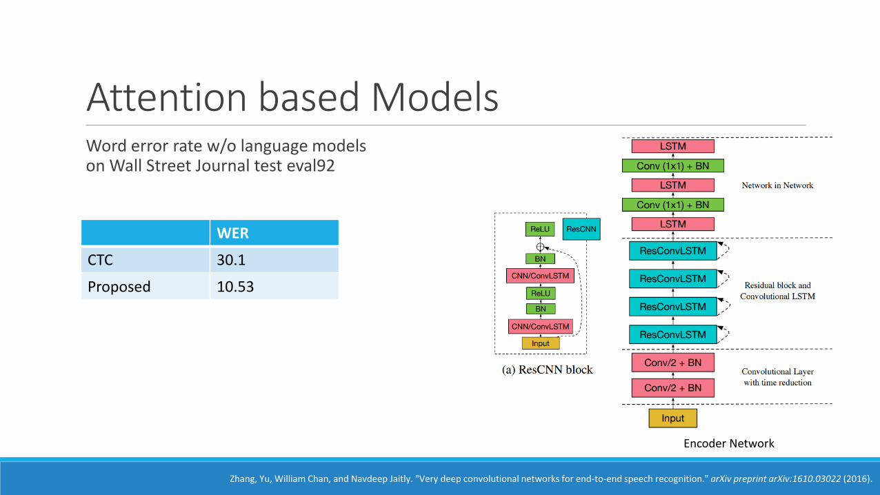
Attention based Models Word error rate w/o language modelson Wall Street Journal test eval92

Zhang, Yu, William Chan, and Navdeep Jaitly. "Very deep convolutional networks for end-to-end speech recognition." arXiv preprint arXiv:1610.03022 (2016).

WER

CTC 30.1

Proposed 10.53

Encoder Network

Deep learning in Speech Recognition

𝑨

FeatureExtraction

FrameClassification

SequenceModel

LexiconModel

LanguageModel


𝑶

GMMs HMMs

𝑸

Sequence States

t ah m aa t ow

𝑳

Phonemes

𝑾

Words Sentence

DNN-HMMsRNN-CTC

Attention

Deep learning in Speech RecognitionTop systems on dataset Switchboard

HMM based system still performs better than End-to-End system on large scale dataset

https://github.com/syhw/wer_are_we

Text to Speech (TTS)

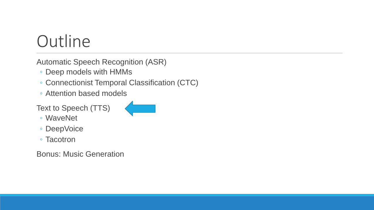
OutlineAutomatic Speech Recognition (ASR)


◦ Connectionist Temporal Classification (CTC)


Text to Speech (TTS)

◦ WaveNet

◦ DeepVoice

◦ Tacotron


Traditional MethodsConcatenative approaches vs. Statistical Parametric approach

◦ Concatenative: More natural sounding, Less flexible, Take up more space

◦ Statistical Parametric: Muffled, more flexible, Smaller models

Traditionally, two stages: frontend and backend

◦ Frontend analyzes text and determines phonemes, stresses, pitch, etc.

◦ Backend generates the audio

Moving towards models which can convert directly from text to audio, with the model itself learning any intermediate representations necessary

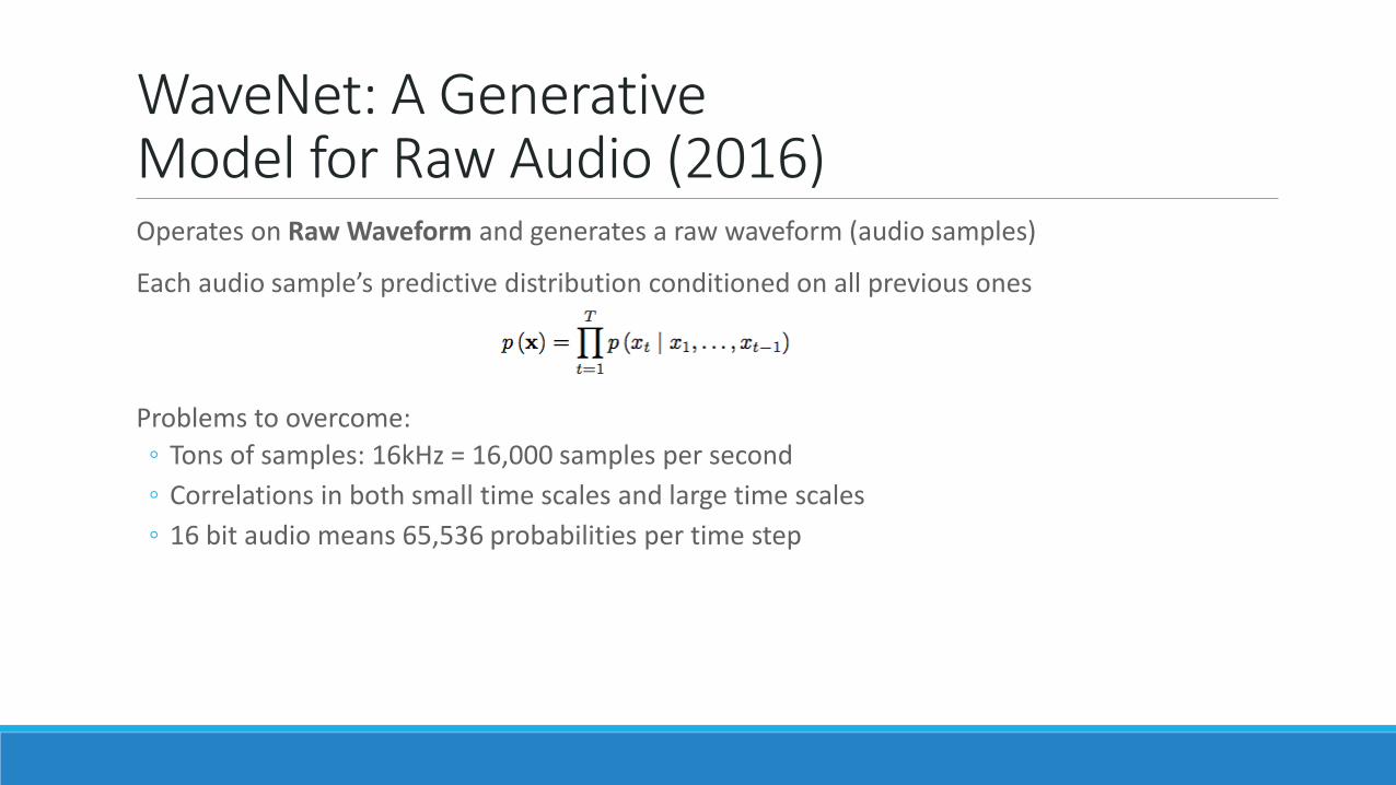
WaveNet: A Generative Model for Raw Audio (2016)Operates on Raw Waveform and generates a raw waveform (audio samples)

Each audio sample’s predictive distribution conditioned on all previous ones

Problems to overcome:

◦ Tons of samples: 16kHz = 16,000 samples per second

◦ Correlations in both small time scales and large time scales

◦ 16 bit audio means 65,536 probabilities per time step

Problem: Too many samples, and different time scales of correlationSolution: Causal Convolutions

https://arxiv.org/pdf/1609.03499.pdf

Causal ConvolutionsPrediction of an audio sample can only depend on timestamps before it (nothing from the future)

No recurrent connections (Not an RNN) => Faster to train than RNN’s

◦ Especially with very long sequences

Glaring problem: Requires many layers to increase the receptive field


Dilated Causal Convolutions


Dilated Causal ConvolutionsFilter is applied to area much larger than its length by skipping inputs at each layer: Large receptive field

Allows information to be gleaned from both temporally close and far samples


Skip connections are used throughout the network

Speeds up convergence

Enables training of deeper models


Where are we now?No input => Generic framework

https://deepmind.com/blog/wavenet-generative-model-raw-audio/


Add in other inputGeneric enough to allow for both universal and local input

◦ Universal: Speaker Identity

◦ Local: Phonemes, inflection, stress

Resultshttps://deepmind.com/blog/wavenet-generative-model-raw-audio/


SampleRNNHow to deal with different time scales? Modularize.

Use different modules operating at different clock rates to deal with varying levels of abstraction

Sample-Level Modules and Frame-Level Modules

https://arxiv.org/abs/1612.07837

Frame-Level Modules“Each frame-level module is a deep RNN which summarizes the history of its inputs into a conditioning vector for the next module downward.”

Each module takes as input its corresponding frame, as well as the conditioning vector of the layer above it.

Sample Level ModulesConditioned on the conditioning vector from the frame above it, and on some number of preceding samples.

Since this number is generally small, they use a multilayer perceptron here instead of an RNN, to speed up training

“When processing an audio sequence, the MLP is convolved over the sequence, processing each window of samples and predicting the next sample.”

“At generation time, the MLP is run repeatedly to generate one sample at a time.”

Other aspects of SampleRNNLinear Quantization with q=256

RNN’s (not used in WaveNet) are powerful if they can be trained efficiently

Truncated Back Propagation Through Time (BPTT)

◦ Split sequence into subsequences and only propagate gradient to beginning of subsequence

◦ Interestingly, able to train well on subsequences of only 32ms

Resultshttps://soundcloud.com/samplernn

https://soundcloud.com/samplernn

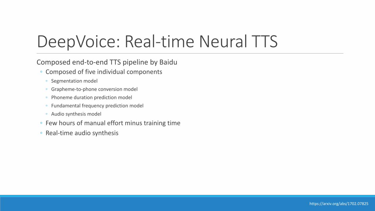
DeepVoice: Real-time Neural TTSComposed end-to-end TTS pipeline by Baidu

◦ Composed of five individual components◦ Segmentation model

◦ Grapheme-to-phone conversion model

◦ Phoneme duration prediction model

◦ Fundamental frequency prediction model

◦ Audio synthesis model

◦ Few hours of manual effort minus training time

◦ Real-time audio synthesis


DeepVoice Grapheme-to-Phoneme ModelEncoder-decoder architecture from “Sequence-to-Sequence Neural Net Models for Grapheme-to-Phoneme Conversion”

Architecture◦ Trained with teacher forcing

◦ Decode phonemes with beam search of width 5

10

24

GR

U U

nit

s

10

24

GR

U U

nit

s

10

24

GR

U U

nit

s

Text

Inp

ut

10

24

GR

U U

nit

s

10

24

GR

U U

nit

s

10

24

GR

U U

nit

s

Ph

on

em

es

Bidirectional encoder

Unidirectional decoder


DeepVoice Segmentation ModelConvolutional recurrent neural network architecture from “DeepSpeech 2: End-to-End Speech Recognition in English and Mandarin”

Architecture◦ 2D convolutions in time and frequency

◦ Softmax layer uses CTC to predict phoneme pairs◦ Output spikes from CTC close to phoneme

boundaries

◦ Decode phoneme boundaries with beam search of width 50

Bidirectional RNN layers

51

2 G

RU

Un

its

51

2 G

RU

Un

its

Soft

max

ou

tpu

t w

/ C

TC

Ph

on

em

e D

ura

tio

ns

Convolutional layers

Featurized Audio

10 ms

20

MFC

C


DeepVoice Phoneme Duration and Fundamental Frequency ModelOutputs

◦ Phoneme duration

◦ Probability phoneme is voiced (has F0)

◦ 20 time-dependent F0 values

Loss

𝐿𝑛 = Ƹ𝑡𝑛 − 𝑡𝑛 + 𝜆1CE ො𝑝𝑛, 𝑝𝑛 + 𝜆2

𝑡=0

𝑇−1

𝐹0𝑛,𝑡 − 𝐹0𝑛,𝑡

+𝜆3

𝑡=0

𝑇−2

|𝐹0𝑛,𝑡+1 − 𝐹0𝑛,𝑡|

◦ 𝜆𝑖 are tradeoff constants

◦ Ƹ𝑡𝑛, 𝑡𝑛 are durations of 𝑛𝑡ℎ phoneme

◦ ො𝑝𝑛, 𝑝𝑛 are probabilities 𝑛𝑡ℎ phoneme is voiced

◦ 𝐹0𝑛,𝑡, 𝐹0𝑛,𝑡 are fundamental frequency of 𝑛𝑡ℎ phoneme

25

6 U

nit

s

25

6 U

nit

s

On

e-h

ot

ph

on

eme

w/

stre

ss v

ecto

r

12

8 G

RU

Un

its

FC O

utp

uts

Fully connected layers

Unidirectional layers

12

8 G

RU

Un

its


DeepVoice Audio Synthesis ModelArchitecture

◦ Red WaveNet◦ Same structure, different 𝑙, 𝑟, 𝑠 values

◦ Blue Conditioning network◦ Two bidirectional QRNN layers

◦ Interleave channels

◦ Upsample to 16kHZ


DeepVoice Training

Grapheme-to-Phoneme model used as backup to phoneme dictionary (CMUdict)


DeepVoice Inference

Segmentation model only annotates data in training and not used in inference


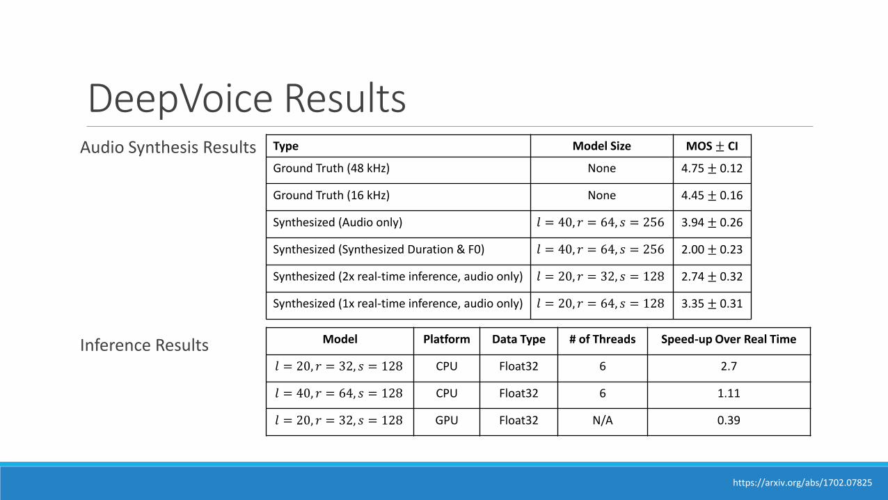
DeepVoice ResultsAudio Synthesis Results

Inference Results

Type Model Size MOS ± CI

Ground Truth (48 kHz) None 4.75 ± 0.12


Synthesized (Audio only) 𝑙 = 40, 𝑟 = 64, 𝑠 = 256 3.94 ± 0.26

Synthesized (Synthesized Duration & F0) 𝑙 = 40, 𝑟 = 64, 𝑠 = 256 2.00 ± 0.23

Synthesized (2x real-time inference, audio only) 𝑙 = 20, 𝑟 = 32, 𝑠 = 128 2.74 ± 0.32


Model Platform Data Type # of Threads Speed-up Over Real Time

𝑙 = 20, 𝑟 = 32, 𝑠 = 128 CPU Float32 6 2.7

𝑙 = 40, 𝑟 = 64, 𝑠 = 128 CPU Float32 6 1.11

𝑙 = 20, 𝑟 = 32, 𝑠 = 128 GPU Float32 N/A 0.39


DeepVoice Implementation DetailsCPU implementation

◦ Parallelizing work via multithreading

◦ Pinning threads to physical cores (or disabling hyperthreading)

◦ Replacing nonlinearities with high-accuracy approximations (only during inference)

tanh 𝑥 ≈ sign 𝑥ǁ𝑒 𝑥 −

1ǁ𝑒 𝑥

ǁ𝑒 𝑥 +1ǁ𝑒 𝑥

and 𝜎 𝑥 ≈

ǁ𝑒 𝑥

1 + ǁ𝑒 𝑥𝑥 ≥ 0

1

1 + ǁ𝑒 𝑥𝑥 ≤ 0

where 𝑒 𝑥 ≈ ǁ𝑒 𝑥 = 1 + 𝑥 + 0.5658𝑥2 + 0.143𝑥4

◦ Weight matrices quantized to int16

◦ Custom AVX assembly kernels for matrix-vector multiplication

GPU implementation◦ Persistant RNNs to generate all samples in one kernel launch

◦ Split model across register file of SMs

◦ Round robin execution of kernels


Tacotron: Towards End-to-End Speech SynthesisTruly end-to-end TTS pipeline by Google

◦ Reduces feature engineering

◦ Allows conditioning on various attributes

Architecture◦ One network based on the sequence-to-

sequence with attention paradigm

◦ Red Encoder

◦ Blue Decoder

◦ Green Post-processing net


Tacotron CBHG Module1D Convolutional Bank + highway network + bidirectional GRU (CBHG)

◦ Module for extracting representations from sequences

◦ Inspired by work from “Fully Character-Level Neural Machine Translation without Explicit Segmentation”

Architecture◦ Bank of 1D convolutional filters

◦ Highway networks◦ Gating unit learn to regulate flow of information through network

◦ Bidirectional GRU RNN


Tacotron EncoderExtracts robust sequential representation of text

Architecture◦ Input: one-hot vector of characters

embedded into a continuous sequence

◦ Pre-Net, a set of on non-linear transformations

◦ CBHG module


Tacotron DecoderTarget is 80-band mel-scale spectrogram rather than raw waveform

◦ Waveform is highly redundant representation

Architecture◦ Attention RNN: 1 layer 256 GRU cells

◦ Decoder RNN: 2 layer residual 256 GRU cells

◦ Fully connected output layer


Tacotron Post-Processing NetworkConvert sequence-to-sequence target to waveform though can be used to predict alternative targets

Architecture◦ CBHG

◦ Griffin-Lim algorithm◦ Estimates waveform from spectrogram

◦ Uses an iterative algorithm to decrease MSE

◦ Used for simplicity


Tacotron ResultsTacotron results

DeepVoice resultsType Model Size MOS ± CI



Synthesized (Audio only) 𝑙 = 40, 𝑟 = 64, 𝑠 = 256 3.94 ± 0.26

Synthesized (Synthesized Duration & F0) 𝑙 = 40, 𝑟 = 64, 𝑠 = 256 2.00 ± 0.23



Model MOS ± CI

Tacotron 3.82 ± 0.085

Parametric 3.69 ± 0.109

Concatenative 4.09 ± 0.119

The quick brown fox jumps over the lazy dog

Generative adversarial network or variational autoencoder

Either way you should shoot very slowly

She set out to change the world and to change us

She set out to change the world and to change us

3)

3)

2)

2)

1)

1)

https://arxiv.org/abs/1702.0782, https://arxiv.org/abs/1703.10135

SummaryAutomatic Speech Recognition (ASR)


◦ Connectionist Temporal Classification (CTC)◦ Method for labeling unsegmented data


Text to Speech (TTS)◦ WaveNet

◦ Audio synthesis network with intermediate representation

◦ DeepVoice◦ Composed end-to-end learning

◦ Tacotron◦ Truly end-to-end learning

Thank you! Questions?

WaveNet, revisitedTrain on 60 hours of Solo YouTube Piano music in one experiment

Train on MagnaTagATune dataset: 29 second clips, 188 tags. No published results unfortunately.



“Deep Learning for Music"Aims to create pleasant music with deep neural nets alone

Questions:

◦ “Is there a meaningful way to represent notes in music as a vector?” (like word2vec)

◦ “Can we build interesting generative neural network architectures that effectively express the

◦ notions of harmony and melody?”

Input

◦ Midi Data

◦ Piano Roll data (which notes are on?)

The Network2 Layer LSTM

Map tokens (either MIDI messages or note combinations) to a learned vector respresentation

Feed output into softmax layer

Allows user to adjust hyperparamters including number of layers, hidden unit size, sequence length, batch size, and learning rate.

Input a “seed” sequence

Two approaches to generation:

◦ Choose maximum from softmax

◦ Choose anything from the softmax distribution

ResultsMusic trained solely on Bach was better than a mix of classical pianists

Music trained using the Piano Roll format was better than that of the MIDI messages

No published audio, unfortunately

ReferencesText to Speech (TTS)

◦ A. van den Oord, S. Dieleman, H. Zen, K. Simonyan, O. Vinyals, A. Graves, N. Kalchbrenner, A. Senior, and K. Kavukcuoglu. WaveNet: A Generative Model for Raw Audio. arXiv preprint arXiv:1609.03499 (2016).

◦ S. Mehri, K. Kumar, I. Gulrajani, R. Kumar, S. Jain, J. Sotelo, A. Courville, and Y. Bengio. SampleRNN: An Unconditional End-to-End Neural Audio Generation Model. arXiv preprint arXiv:1612.07837v2 (2017).

◦ J. Sotelo, S. Mehri, K. Kumar, J. Santos, K. Kastner, A. Courville, and Y. Bengio. Char2Wav: End-to-End Speech Synthesis. ICLR (2017).

◦ S. Arik, M. Chrzanowski, A. Coates, G. Diamos, A. Gibiansky, Y. Kang, X. Li, J. Miller, A. Ng, J. Raiman, S. Sengupta, and M. Shoeybi. Deep Voice: Real-time Neural Text-to-Speech. arXiv preprint arXiv:1702.07825v2 (2017).

◦ Y. Wang, and et al. Tacotron: A Fully End-to-End Text-to-Speech Synthesis Model. arXiv preprint arXiv:1703.10135v1 (2017).



https://mila.umontreal.ca/en/publication/char2wav-end-to-end-speech-synthesis/



ReferencesAutomatic Speech Recognition (ASR)

◦ A. Graves, S. Fernandez, F. Gomez, and J. Schmidhuber. Connectionist Temporal Classification: Labelling Unsegmented Sequence Data with Recurrent Neural Networks. ICML (2006).

◦ G. Hinton, et al. Deep Neural Networks for Acoustic Modeling in Speech Recognition. Signal Processing Magazine (2012).◦ A. Graves, A. Mohamed, and G. Hinton. Speech Recognition with Deep Recurrent Neural Networks. arXiv preprint

arXiv:1303.5778v1 (2013).◦ H. Sak, A. Senior, and F. Beaufays. Long Short-Term Memory Recurrent Neural Network Architectures for Large Scale Acoustic

Modeling.. rXiv preprint arXiv:1402.1128v1 (2014).◦ O.Abdel-Hamid, et al. Convolutional Neural Networks for Speech Recognition. IEEE/ACM Transactions on Audio, Speech, and

Language Processing (2014).◦ A. Hannun, C. Case, J. Casper, B. Catanzaro, G. Diamos, E. Elsen, R. Prenger, S. Satheesh, S. Sengupta, A. Coates, and A.

Ng. Deep Speech: Scaling up end-to-end speech recognition. arXiv preprint arXiv:1412.5567v2 (2014).◦ D. Amodei, et al. Deep Speech 2: End-to-End Speech Recognition in English and Mandarin. arXiv preprint arXiv:1512.02595v1

(2015).◦ Y. Wang. Connectionist Temporal Classification: A Tutorial with Gritty Details. Github (2015).◦ D. Bahdanau, et al. End-to-End Attention-based Large Vocabulary Speech Recognition. arXiv preprint arXiv:1508.04395

(2015).◦ W. Xiong, et al. Achieving Human Parity in Conversational Speech Recognition. arXiv preprint arXiv:1610.05256 (2016).

ftp://ftp.idsia.ch/pub/juergen/icml2006.pdf

https://www.microsoft.com/en-us/research/wp-content/uploads/2016/02/HintonDengYuEtAl-SPM2012.pdf



http://ieeexplore.ieee.org/document/6857341/



https://github.com/yiwangbaidu/notes/blob/master/CTC/CTC.pdf

https://arxiv.org/pdf/1508.04395


ReferencesMusic Generation

◦ A. Huang, and R. Wu. Deep Learning for Music. arXiv preprint arXiv:1606.04930v1 (2016).

◦ V. Kaligeri, and S. Grandhe. Music Generation Using Deep Learning. arXiv:1612.04928v1 (2016).



deep learning for audio - university of...

Documents