decrease and conquer - funny funny algorithm...
TRANSCRIPT


Decrease and Conquer
1. Reduce a problem instance to a smaller instance of the same problem and extend solution
2. Solve the smaller instance
3. Extend solution of smaller instance to obtain solution to original problem
• Also referred to as inductive, incremental approach or chip and conquer
3 / 82

Examples of Decrease & Conquer
• Decrease by one: – Insertion sort – Graph search algorithms:
• DFS • BFS • Topological sorting
– Algorithms for generating permutations, subsets
• Decrease by a constant factor – Binary search – Fake-coin problems – multiplication à la russe – Josephus problem
• Variable-size decrease – Euclid’s algorithm – Selection by partition
4 / 82
What’s the difference?
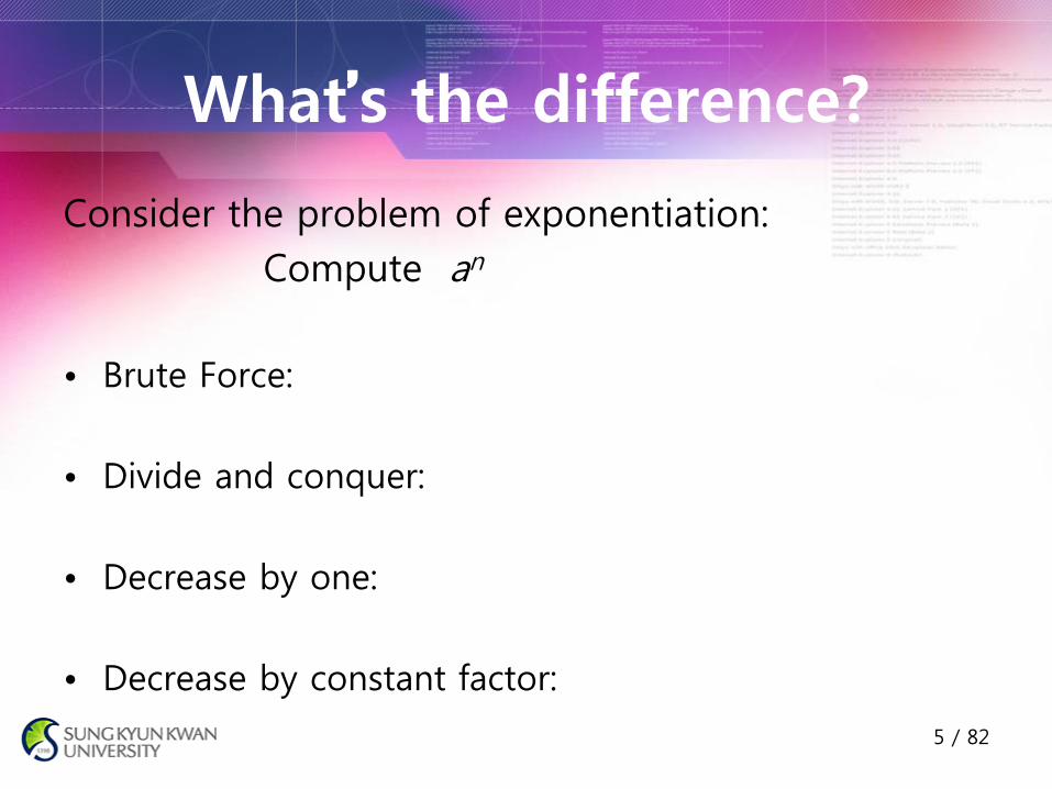
Consider the problem of exponentiation:
Compute an
• Brute Force:
• Divide and conquer:
• Decrease by one:
• Decrease by constant factor:
5 / 82

What’s the difference?
Consider the problem of exponentiation:
Compute an
• Brute Force: an= a*a*a*a*...*a
• Divide and conquer: an= an/2 * an/2
• Decrease by one: an= an-1* a
• Decrease by constant factor: an= (an/2)2
6 / 82

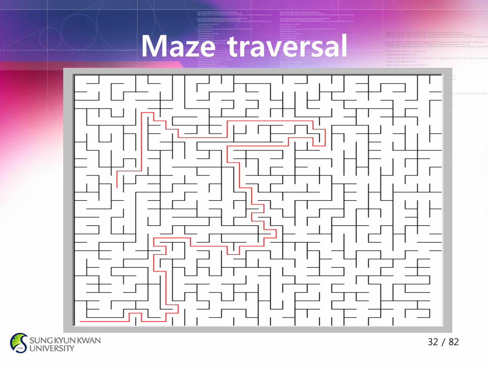
Graph Traversal
• Many problems require processing all graph vertices in systematic fashion
• Graph traversal algorithms:
– Depth-first search
– Breadth-first search
• First, some definitions!
8 / 82

Graphs • A (simple) graph G = (V, E) consists of
– V, a nonempty set of vertices
– E, a set of unordered pairs of distinct vertices called edges.
• Examples:
9 / 82

Directed Graphs • A directed graph (digraph) G = (V, E) consists of
– V, a nonempty set of vertices
– E, a set of ordered pairs of distinct vertices called edges.
• Examples:
10 / 82

Weighted Graph • A weighted graph is a triple G = (V, E, W)
– where (V, E) is a graph (or a digraph) and
– W is a function from E into R, the reals (integer or rationals).
– For an edge e, W(e) is called the weight of e.
• A weighted digraph is often called a network.
• Examples
11 / 82

Graph Terminology • Let u and v be vertices, and let e = (u,v) be an
edge in an undirected graph G. – The vertices u and v are adjacent.
– The edge e is incident with both vertices u and v.
– The edge e connects u and v.
– The vertices u and v are the endpoints of edge e.
– The degree of a vertex, denoted deg(v), in an undirected graph is the number of edges incident with it (where self-loops are counted twice).
12 / 82


More Graph Terminology • A subgraph of a graph G = (V, E) is a graph
G = (V, E) such that V V and E E.
(a simple path)
A path is a sequence of vertices v1, v2, v3, …, vk such that consecutive vertices vi and vi+1 are adjacent.
15 / 82

Graph Representations using Data Structures
• Adjacency Matrix Representation – Let G = (V, E), n = |V|, m = |E|, V = {v1, v2, …, vn)
– G can be represented by an n n matrix C
16 / 82


More Definitions • Subgraph • Symmetric digraph • Complete graph • Adjacency relation • Path, simple path, reachable • Connected, Strongly Connected • Cycle, simple cycle • Acyclic • Undirected forest • Free tree, undirected tree • Rooted tree • Connected component
20 / 82

Traversing Graphs • Most algorithms for solving problems on a
graph examine or process each vertex and each edge.
• Depth-First Search (DFS) and Breadth-First Search (BFS) – Two elementary traversal strategies that provide an
efficient way to “visit” each vertex and edge exactly once.
– Both work on directed or undirected graphs.
– Many advanced graph algorithms are based on the concepts of DFS or BFS.
– The difference between the two algorithms is in the order in which each “visits” vertices.
21 / 82


Depth-first search • Explore graph always moving away from last visited
vertex
• Pseudocode for Depth-first-search of graph G=(V,E)
dfs(v)
count := count + 1
mark v with count
for each vertex w adjacent to v do
if w is marked with 0
dfs(w)
DFS(G)
count :=0
mark each vertex with 0 (unvisited)
for each vertex v V do
if v is marked with 0
dfs(v)
23 / 82
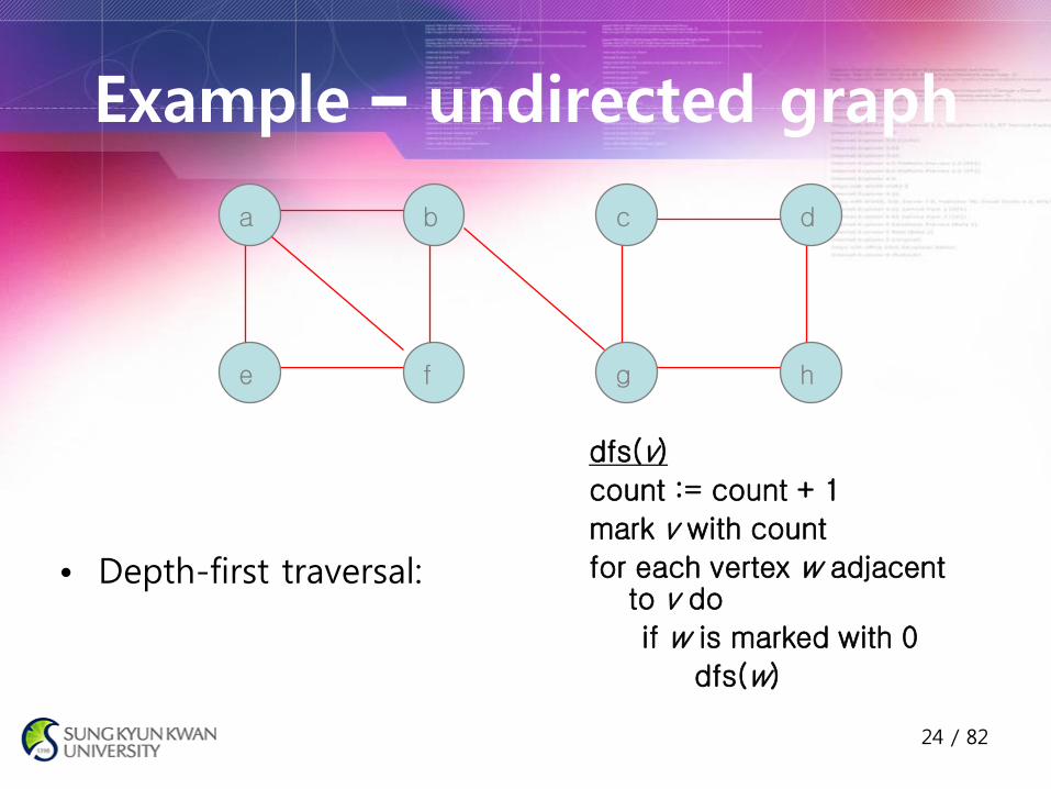
Example – undirected graph
• Depth-first traversal:
a b
e f
c d
g h
dfs(v)
count := count + 1
mark v with count
for each vertex w adjacent to v do
if w is marked with 0
dfs(w)
24 / 82


Types of edges
• Tree edges: edges comprising forest
• Back edges: edges to ancestor nodes
26 / 82

Question
• How to rewrite the procedure dfs(v), using a stack to eliminate recursion
dfs(v)
count := count + 1
mark v with count
for each vertex w adjacent to v do
if w is marked with 0
dfs(w)
27 / 82

Non-recursive version of DFS algorithm
Algorithm dfs(v)
s.createStack(); s.push(v); count := count + 1 mark v with count while (!s.isEmpty()) { let x be the node on the top of the stack s; if (no unvisited nodes are adjacent to x) s.pop(); // backtrack else { select an unvisited node u adjacent to x; s.push(u); count := count + 1 mark u with count } }
28 / 82

DFS stack and forest
a1,8 b2,7 f3,2 e4,1
g5,6 c6,5 d7,4 h8,3
preorder: a b f e g c d h
postorder: e f h d c g b a
a b
e f
c d
g h
a
b
e
f c
d
g
h 29 / 82

Depth-first search: Notes
• Yields two distinct ordering of vertices: – preorder: as vertices are first encountered (pushed onto stack)
– postorder: as vertices become dead-ends (popped off stack)
• Applications: – checking connectivity, finding connected components
– checking acyclicity
– searching state-space of problems for solution (AI)
30 / 82

In-class Exercise • Consider the graph
a. Write down the adjacency matrix and adjacency lists specifying this
graph. (Assume that the matrix rows and columns and vertices in the
adjacency lists follow in the alphabetical order of the vertex labels.)
b. Starting at vertex A and resolving ties by the vertex alphabetical order,
traverse the graph by depth-first search and construct the corresponding
depth-first search tree. Give the order in which the vertices were reached
for the first time (pushed onto the traversal stack) and the order in which
the vertices became dead ends (popped off the stack).
31 / 82


Breadth-first search
• Explore graph moving across to all the neighbors of last visited vertex
• Similar to level-by-level tree traversals
• Instead of a stack, breadth-first uses queue
• Applications: same as DFS, but can also find paths from a vertex to all other vertices with the smallest number of edges
35 / 82
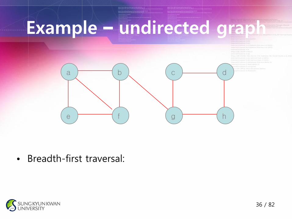
Example – undirected graph
• Breadth-first traversal:
a b
e f
c d
g h
36 / 82

BFS queue and forest
• a b e f g c h d
a b
e f
c d
g h
a
b e f
c
d
g
h
37 / 82

Breadth-first search algorithm bfs(v)
count := count + 1
mark v with count
initialize queue with v
while queue is not empty do
a := front of queue
for each vertex w adjacent to a do
if w is marked with 0
count := count + 1
mark w with count
add w to the end of the queue
remove a from the front of the queue
BFS(G) count :=0 mark each vertex with 0
for each vertex v V do if v is marked with 0
bfs(v)
38 / 82
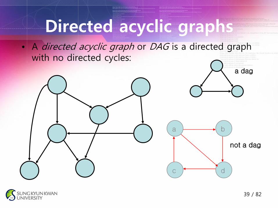
Directed acyclic graphs • A directed acyclic graph or DAG is a directed graph
with no directed cycles:
a b
c d
not a dag
a dag
39 / 82
Directed acyclic graphs (DAG)
• Arise in many modeling problems, e.g.:
– course prerequisite structure
– food chains
• Imply partial ordering on the domain
40 / 82

Topological Sort
• Topological sort of a DAG: – Linear ordering of all vertices in graph G
such that for every edge (u, v) G, the vertex, u, where the edge starts is listed before the vertex, v, where the edge ends.
cs101
cs203
math101
cs310
cs401
cs825
cs525
cs990
41 / 82

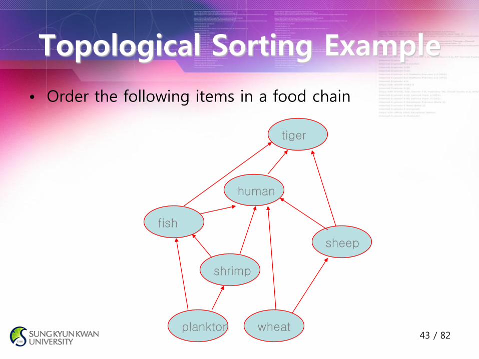
Topological Sorting Example
• Order the following items in a food chain
fish
human
shrimp
sheep
wheat plankton
tiger
43 / 82

Topological sorting Algorithms
1. DFS-based algorithm: – DFS traversal noting order vertices are popped off stack
– Reverse order solves topological sorting
– Back edges encountered?→ NOT a dag!
2. Source removal algorithm – Repeatedly identify and remove a source vertex, ie, a vertex
that has no incoming edges
44 / 82

Question
• How would you find a source (or determine that such a vertex does not exist) in a digraph
– represented by adjacency matrix?
– represented by adjacency linked list?
45 / 82


Decrease by a constant factor - Examples
• Fake-coin problem
• Multiplication à la russe (Russian peasant method)
• Josephus problem
47 / 82

Fake-Coin Puzzle (simpler version)
There are n identically looking coins one of which is fake. There is a balance scale but there are no weights; the scale can tell whether two sets of coins weigh the same and, if not, which of the two sets is heavier (but not by how much). Design an efficient algorithm for detecting the fake coin. Assume that the fake coin is known to be lighter than the genuine ones.
Decrease by factor 2 algorithm
Decrease by factor 3 algorithm

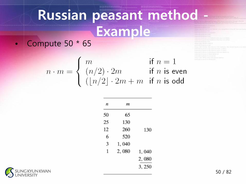
Russian peasant method
• n*m
• If n is even, n*m = (n/2)*(2m)
• If n is odd, n*m = ((n-1)/2)*(2m)+m
• Repeat the above process until we have the trivial case of 1*x = x
• Only simple operations: halving, doubling, and adding, no need to memorize the table of multiplications
49 / 82

Josephus problem
• Josephus Flavius Game – Josephus Flavius was a famous Jewish historian of the first
century at the time of the Second Temple destruction. During the Jewish-Roman war he got trapped in a cave with a group of 40 soldiers surrounded by romans. The legend has it that preferring suicide to capture, the Jews decided to form a circle and, proceeding around it, to kill every third remaining person until no one was left. Josephus, not keen to die, quickly found the safe spot in the circle and thus stayed alive.
51 / 82

Decrease by a variable size - Examples
• Euclid’s algorithm for greatest common divisor
• Selection problem
• Binary search tree
53 / 82

Euclid’s algorithm for greatest common divisor
• 50 : 1, 2, 5, 10, 25, 50
20 : 1, 2, 4, 5, 10, 20
• GCD(x, y) = GCD(x-y, y)
GCD(x,y) = GCD(y,x)
Ex) GCD(50,20) = GCD(30,20) = GCD(10,20) = GCD(20,10) =
GCD(10,10) = GCD(0,10) = GCD(10,0)
• GCD(X,Y) = GCD(X%Y, Y)
Ex) GCD(50,20) = GCD(10,20) = GCD (20,10) = GCD(0,10)
54 / 82

Euclid’s algorithm for greatest common divisor
• Steps for 2 natural numbers n and m
– E1 : r ← m mod n;
– E2 : if ( r = 0 ) then return;
– E3 : m ← n; n ← r;
55 / 82
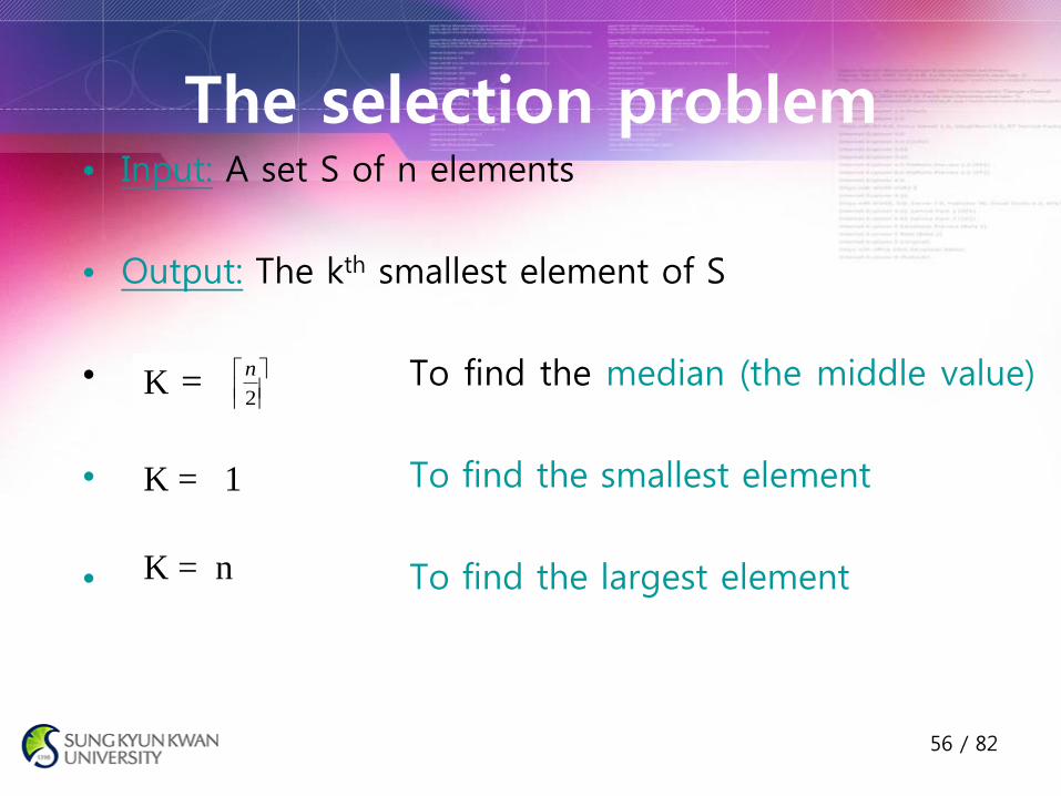
The selection problem • Input: A set S of n elements
• Output: The kth smallest element of S
• To find the median (the middle value)
• To find the smallest element
• To find the largest element
K = 1
K = n
K =
2
n
56 / 82

The selection problem
• Input: A set S of n elements
• Output: The kth smallest element of S
• The straightforward algorithm:
– step 1: Sort the n elements
– step 2: Locate the kth element in the sorted list.
This algorithm is overkill!
57 / 82

Search problem • Search a key in a sorted list
– Sequential search
– Binary search
• How do you search for a name in a telephone book?
– Using binary search
58 / 82
Binary Search Trees (BSTs)
• Binary Search Tree property – A binary tree in which the key of an internal node is greater
than the keys in its left subtree and less than or equal to the keys in its right subtree.
• An inorder traversal of a binary search tree produces a sorted list of keys.
59 / 82

Variable-size-decrease: Binary search trees
• Keys are arranged in a binary tree with the binary search tree property:
k
<k k
60 / 82

BST Examples • Binary Search trees with different degrees of balance
• Black dots denote empty trees
• Size of a search tree 61 / 82

Variable-size-decrease: Binary search trees
• Arrange keys in a binary tree with the binary search tree property:
k
<k k
Example 1: 5, 10, 3, 1, 7, 12, 9 Example 2: 4, 5, 7, 2, 1, 3, 6
62 / 82

BST Operations
• Find the min/max element ()
• Search for an element
• Find the successor/predecessor of an element
• Insert an element
• Delete an element
63 / 82

BST: Min/Max • The minimum element is the left-most node
x is a non-empty BST
The maximum element is the right-most node
64 / 82

BST Operations
• Find the min/max element
• Search for an element ()
• Find the successor/predecessor of an element
• Insert an element
• Delete an element
65 / 82

BST Search (Retrieval) Element bstSearch(BinTree bst, Key K)
1. Element found
2. if (bst == nil)
3. found = null;
4. else
5. Element root = root(bst);
6. if (K == root.key)
7. found = root;
8. else if (K < root.key)
9. found = bstSearch (leftSubtree(bst), K);
10. else
11. found = bstSearch(rightSubtree(bst), K);
12. return found;
66 / 82

BST Operations
• Find the min/max element
• Search for an element
• Find the successor/predecessor of an element ()
• Insert an element
• Delete an element
67 / 82

BST: Successor/Predecessor
• Finding the successor of a node x (if it exists): – If x has a nonempty right subtree, then successor(x) is the
smallest element in the tree root at rightSubtree(x)
68 / 82
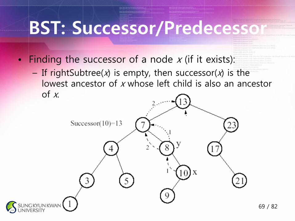
BST: Successor/Predecessor
• Finding the successor of a node x (if it exists):
– If rightSubtree(x) is empty, then successor(x) is the lowest ancestor of x whose left child is also an ancestor of x.
69 / 82

Why binary search tree?
Array: 1 3 4 5 7 8 9 10 13 17 21 23
BST:
70 / 82
BST: advantage
• The advantage to the binary search tree approach is that it combines the advantage of an array--the ability to do a binary search with the advantage of a linked list--its dynamic size.
71 / 82

BST Operations
• Find the min/max element
• Search for an element
• Find the successor/predecessor of an element
• Insert an element ()
• Delete an element
72 / 82

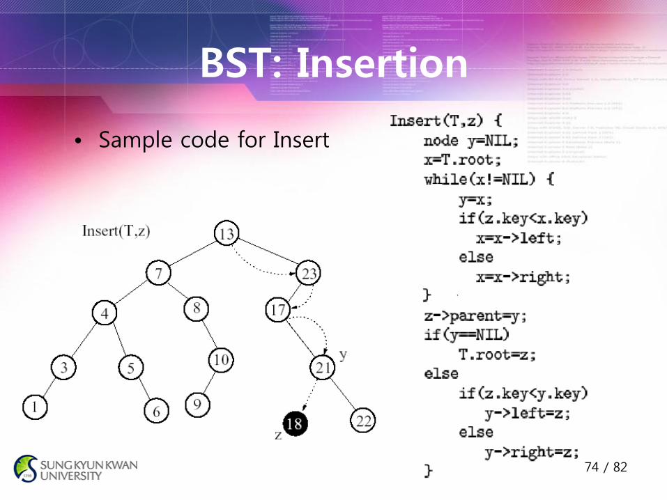
BST: Insertion
• To insert a node into a BST, we search the tree until we find a node whose appropriate subtree is empty, and insert the new node there.
73 / 82

BST Operations
• Find the min/max element
• Search for an element
• Find the successor/predecessor of an element
• Insert an element
• Delete an element ()
75 / 82

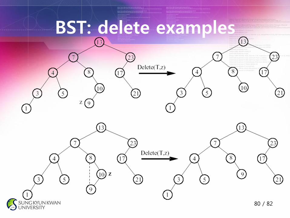
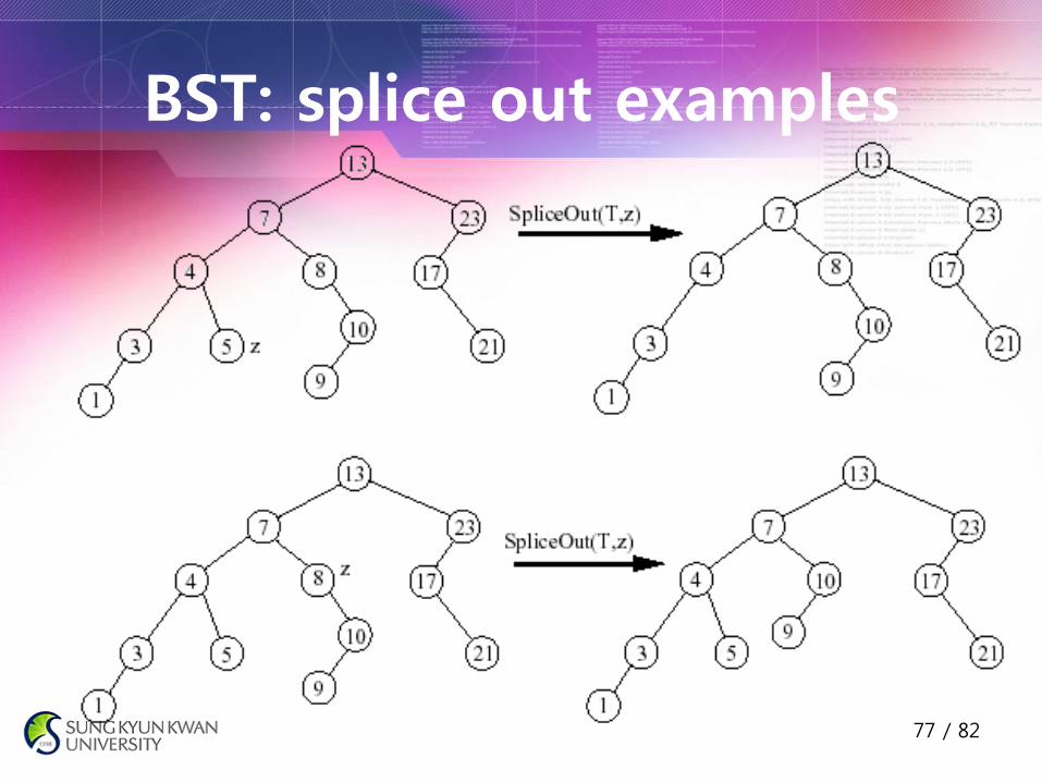
BST: Delete
• Deleting a node z is by far the most difficult BST operation.
• There are three cases to consider – If z has no children, just delete it.
– If z has one child, splice out z, That is, link z’s parent and child
– If z has two children, splice out z’s successor y, and replace the contents of z with the contents of y
• The last case works because if z has two children, then its successor has no left child
76 / 82
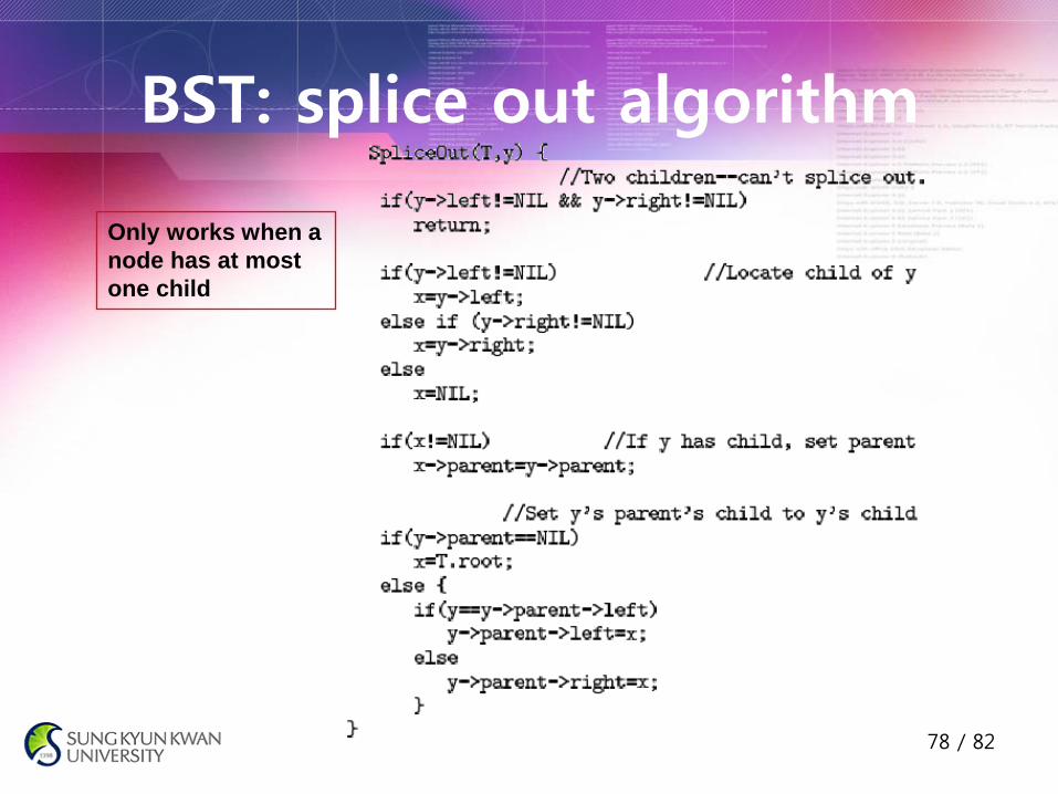
BST: splice out algorithm
Only works when a
node has at most
one child
78 / 82