Chair of Industrial Information Technology

Institute for Machine Tools and Factory Management (IWF)

Supervisors:

Prof. Dr.-Ing. R. Stark

Dip.–Ing. Anne Pförtner

Bachelor Thesis

Decision support for sustainable product design based on an automatized FEM

analysis

Martin Iradi, Bernardo Matriculation number: 369423 18.8.2015

1

2

Declaration

I hereby declare that I have developed and written the enclosed bachelor thesis by myself. The sources and aids I have used are indicated in the text. Bernardo Martin August 2015

3

Gratitudes

Personally, I would like to thank to the Dipl.-Ing. Anne Pförtner for accept being my

tuthor and giving me the opportunity of working inside this rich and interesting project.

Also, I would like to thank to the whole personnel of the Institut für

Werkzeugmaschinen und Fabrikbetrieb (IWF), specially, to Thomas Meischner and

Dipl.-Ing. Thomas Vorsatz for helping me solving different issues during the process.

4

Index 1. INTRODUCTION .................................................................................................................... 9

1.1. Motivation .................................................................................................................... 9

1.2. Research Method ....................................................................................................... 9

1.3. Thesis Structure ........................................................................................................ 10

2. FEM ANALYSIS ................................................................................................................... 11

2.1. Process of an FEA ................................................................................................... 11

2.1.1. Pre-process ....................................................................................................... 11

2.1.2. Analysis .............................................................................................................. 14

2.1.3. Post-process ..................................................................................................... 15

2.2. Examples of uses of FEA ........................................................................................ 15

2.3. Relevant parameters to set an FEM model .......................................................... 16

2.3.1. Geometry of the elements forming the mesh ............................................... 16

2.3.2. Type of solver .................................................................................................... 18

2.3.3. Analysis type ..................................................................................................... 19

2.3.4. Type of solution................................................................................................. 20

3. FUNCTIONS IN NX .......................................................................................................... 22

3.1. Functions and parameters to perform FEM analysis .......................................... 22

3.1.1. Modelling features ............................................................................................ 22

3.1.2. FEM and Simulation settings .......................................................................... 24

3.1.3. Meshing features .............................................................................................. 26

3.1.4. Different Constraints ........................................................................................ 29

3.1.5. Post processing features ................................................................................. 29

3.2. Material database ..................................................................................................... 30

3.2.1. Type of materials .............................................................................................. 31

3.2.2. Material categories ........................................................................................... 31

3.2.3. Non linearity of materials ................................................................................. 32

3.2.4. Material library in NX 9.0 ................................................................................. 32

4. IMPLEMENTATION OF AN AUTOMATIC FEM ANALYSIS ..................................... 34

4.1. Goals and concept of the implementation ............................................................ 34

4.1.1. Procedure of the implementation ................................................................... 34

4.1.2. Selection of materials ....................................................................................... 37

4.1.3. Geometrical restrictions and final model ....................................................... 40

4.1.4. Characteristics and restrictions of the FEM analysis .................................. 47

4.2. Calculus time of the results ..................................................................................... 54

5. CONCLUSION .................................................................................................................. 55

5

5.1. Interpretation and study of the obtained results. ................................................. 55

5.2. Outlook ....................................................................................................................... 58

REFERENCES ......................................................................................................................... 59

Bibliographic references ...................................................................................................... 59

Online resources .................................................................................................................. 59

APPENDIX ................................................................................................................................ 62

6

Figure Index

Figure 1. Diagram showing the different steps of a FEA analysis ............................................... 11

Figure 2. Refinement of a mesh following the Bias argument. ................................................... 13

Figure 3. The same model meshed with different sizes. ............................................................ 13

Figure 4. The three main axes and their rotations. ..................................................................... 14

Figure 5. FEM of an aircraft. ........................................................................................................ 16

Figure 6. FEM of a shovel. ........................................................................................................... 16

Figure 7. FEM of a race car against the wind. ............................................................................. 16

Figure 8. FEM of a car collision. .................................................................................................. 16

Figure 9. FEM of a local weather prediction. .............................................................................. 16

Figure 10. 1D elements. .............................................................................................................. 17

Figure 11. 2D triangular elements. ............................................................................................. 17

Figure 12. 2D rectangular elements. ........................................................................................... 17

Figure 13. 3D tetrahedral elements. ........................................................................................... 17

Figure 14. 3D cubic elements. ..................................................................................................... 18

Figure 15. Structural analysis example. ...................................................................................... 19

Figure 16. Thermal analysis example. ......................................................................................... 19

Figure 17. Example of nonlinear solution. .................................................................................. 20

Figure 18. Diagram strain-stress of a material behavior. ............................................................ 21

Figure 19. Sketch designing toolbar. ........................................................................................... 22

Figure 20. Geometry designing toolbar. ..................................................................................... 23

Figure 21. Geometry idealization possibilities. ........................................................................... 23

Figure 22. New FEM and simulation panel of NX 9.0. ................................................................. 24

Figure 23. Geometry options panel of NX 9.0. ............................................................................ 24

Figure 24. Solution settings panel of NX 9.0. .............................................................................. 25

Figure 25. Free mesh and Mapped mesh examples. .................................................................. 26

Figure 26. Different meshes available in NX 9.0. ........................................................................ 27

Figure 27. 1D Mesh panel of NX 9.0 ............................................................................................ 27

Figure 28. Load type panel of NX 9.0. ......................................................................................... 29

Figure 29. Constraint type panel of NX 9.0. ................................................................................ 29

Figure 30. Different results available in NX 9.0. .......................................................................... 30

Figure 31. Different behavior of materials depending on the direction. .................................... 31

Figure 32. Ceramic material (tile)................................................................................................ 31

Figure 33. Metalic objects ........................................................................................................... 32

7

Figure 34. A car tire. .................................................................................................................... 32

Figure 35. Plastic envases. .......................................................................................................... 32

Figure 36. Master model of the original Tripelec frame. ............................................................ 41

Figure 37. Variation of singularities. ........................................................................................... 42

Figure 38. Model of the central frame in 3D............................................................................... 43

Figure 39. Sketch of the central frame in 1D. ............................................................................. 44

Figure 40. Model of the whole final frame in 1D. ....................................................................... 44

Figure 41. Model of the final frame with the mesh applied. ...................................................... 45

Figure 42. First sketch. ................................................................................................................ 45

Figure 43. Second sketch. ........................................................................................................... 46

Figure 44. Third sketch. ............................................................................................................... 46

Figure 45. Fourth sketch. ............................................................................................................ 47

Figure 46. Result plot with 100 mm element size. ...................................................................... 48

Figure 47. Result plot with 50 mm element size. ........................................................................ 48

Figure 48. Result plot with 20 mm element size. ........................................................................ 49

Figure 49. Result plot with 10 mm element size. ........................................................................ 49

Figure 50. Result plot with 5 mm element size. .......................................................................... 50

Figure 51. Result plot with 2 mm element size. .......................................................................... 50

Figure 52. Master model. ............................................................................................................ 51

Figure 53. Solid mesh. ................................................................................................................. 51

Figure 54. Curves mesh. .............................................................................................................. 51

Figure 55. Master model. ............................................................................................................ 51

Figure 56. Solid mesh. ................................................................................................................. 51

Figure 57. Curves mesh. .............................................................................................................. 51

Figure 58. Master model. ............................................................................................................ 52

Figure 59. Solid mesh. ................................................................................................................. 52

Figure 60. Curves mesh. .............................................................................................................. 52

Figure 61. Final appearance of the applied loads. ...................................................................... 53

Figure 62. Fixed constraint of the front wheel. .......................................................................... 53

Figure 63. Fixed constraint of the bottom curve. ....................................................................... 54

Figure 64. Tungsten. .................................................................................................................... 56

Figure 65. Nodal deformation plot of the tungsten frame. ........................................................ 57

Figure 66. Stress result plot of the tungsten frame. ................................................................... 57

8

Table Index

Table 1. Different sections applicable in 1D Mesh...................................................................... 28

9

1. INTRODUCTION

Within this introduction, the main motivation of the thesis is explained, the research

method used is described and the structure of the thesis is displayed.

1.1. Motivation

The importance of sustainable product development increases due to depleting resources, climate change and increasing inequality among human beings.

Engineers need to be equipped with methods and tools to assess the sustainability of a product and to develop sustainable features directly into the product.

Within the course of the project SFB 1026- sustainable manufacturing and the subproject B1- virtual product creation in sustainable value creation modules a method “ontology based identification of sustainable option (OBISO)” was developed to identify suitable values for product parameters based on given targets. This thesis describes the implementation of one use case for this method. An automatic Finite Element Analysis (FEA) was implemented to identify suitable materials under stiffness and strength conditions. The use case will subsequently be extended to cover also CO2 requirements for wrought material production as well as many other parameters related to a sustainable manufacturing.

The materials will be selected automatically therefore, one of the main benefits this implementation carries is the reduction of time consume spent identifying suitable materials for a model.

In addition, the number of materials tested along the implementation will be adjustable, adding the possibility of testing recently created materials for further studies.

1.2. Research Method

The structure of the thesis follows an efficient organizing methods and is a result of a

deep research in the studied fields.

First of all, a general research about the Finite Element Method was done. This

provided the mathematical and theoretical concepts of the process, as well as

additional knowledge about the tasks that are done in each stage of the analysis.

Secondly, a deep inspection inside the software used during the automation has been

done, acquiring several programming abilities in Java language and identifying the

useful functions of the FEA software (Siemens NX in this case). For programming

knowledge, various help books have been consulted during the study case and for

knowing about the software, it provides itself with a giant platform full of helpful

resources.

Finally, adding all the different previous knowledge obtained, a practical case has been

implemented following a sustainable criteria. Later, its empiric results have been

analyzed, obtaining an overall and reliable conclusion that hopefully will be useful for

coming projects.

10

1.3. Thesis Structure

The structure of the thesis has been based following the standards of every scientific

work. First, the theoretical basis of the study field are explained in detail and

afterwards, they are used to implement a practical case. Therefore, the thesis is

divided into four main chapters:

1. The FEA process.

2. NX features for a FEA.

3. Implementation of the study case.

4. Interpretation of the results and final conclusions.

The first chapter introduces a general perspective of the Finite Element Analysis and

describes how the process takes place and what characterizes the different stages of

the process. Summarizing, is a theoretical approach to the bases of this thesis.

In the second chapter, it is learnt how the NX software is able to perform an FEM

analysis and which are the main functions that are used are explained in detail, as well

as the useful features included in it such as the material library which is used during the

study case.

The next chapter, third one, includes the complete explanation of the implemented use

case. Basically, all the development of the different parts of the automation is

explained. Inside this chapter it is possible to find also which restrictions have limited

the analysis and how the geometry has been adapted to the changing specifications as

well as the application of the constraints to the model and the respective followed

criteria.

Finally, in the last chapter, fourth one, the results are displayed and discussed. At the

end, an overall conclusion is formulated, evaluating the results achieved with the first

set aims and goals, summarizing the whole thesis and making a global balance of it.

11

2. FEM ANALYSIS

An FEM (Finite Element Method) Analysis is used to predict the behavior of structures

subjected to environmental factors such as forces, pressures, heat or vibrations. It

follows a numerical method that generates an approximated solution by differential

equations and it is frequently used in engineering and physics problems as a

computational tool.

When applying the FEA, the complex problem is usually a physical system with the

underlying physics (i.e. Navier-Stokes equations), while the small elements in which

the complex problem is divided represent different areas in the physical system.

2.1. Process of an FEA

The creation of FEM analysis is a process divided into three main steps (Fig.1). The

Pre-process, the Analysis (solver) and the Post-process.

Figure 1. Diagram showing the different steps of a FEA analysis [Peak, 1995].

First, the geometry is created. After it, the piece is divided in elements (mesh) and

applied the different requirements for the analysis (forces, pressures, boundary

conditions...). Finally, the problem is solved and the results are studied in accordance

to the case of study.

2.1.1. Pre-process

The pre-process consists, basically, in defining the geometry of the model, generating

the mesh, applying the boundary conditions and the material properties to it.

2.1.1.1. Geometry

First of all, it is mandatory to set the geometrical specifications and design of the

structure about to analyze. Depending on the type of analysis execution, it is possible

to define 0D (points), 1D (lines), 2D (surfaces) or 3D (volumes) geometries [Roensch,

2013].

-Points: From the FEM analysis point of view, it is useless to work only with them, but

often they help to complement other structures in 1, 2 or 3 dimensions.

12

-Lines: These geometries are more commonly used when analyzing simple objects

such as beams. Although the line is the only visually designed geometry, the type of

profile of the bar should be designed too. Therefore, geometries with constant sections

can be modeled using them, and, as it will be explained later, they can provide high

accurate results.

-Surfaces: Surfaces are more commonly used when the model to analyze has a

constant thickness along its body (i.e. a plastic bottle).

-Volumes: These types of geometries involve a big part of the FEM analysis models.

They are the most versatile ones and can provide with a huge amount of possibilities of

study. They are used to model complex bodies and nowadays, using the computer

software, it is possible to create almost every geometry.

In addition to that, the different dimensional geometries described before can be

combined forming what it is knows as assemblies. This allows connecting different sub

geometries forming a final main one.

2.1.1.2. The mesh

The next part is the generation of the mesh. Usually this is the most time consuming

task of the FEA and it consists in dividing the model into many finite elements that are

formed by points called nodes and it is also known as a form of domain discretization.

As it will be explained later, the elements forming the mesh could vary in geometry,

dimension and behavior depending on the purpose of the analysis.

As well as the geometry, it is possible to mesh 1D geometries (wireframe), with points

and curves representing edges; 2D geometries (surfaced), with surfaces defining

boundaries; or the most common ones, 3D geometries (solid), defining where the

material is.

Most of the FEA software mesh the geometry with a mapping algorithm or an automatic

free-meshing algorithm. The first, maps a rectangular grid onto a geometric region,

which should have the right number of sides. Mapped meshes are suitable for simple

3D solids (i.e. bricks) but often very time-consuming and usually impossible to apply to

complex geometries. Free meshing automatically divides meshing regions into

elements, with the advantage of fast meshing, easy mesh-size transitioning and

adaptive capabilities. However, disadvantages include generation of distorted elements

and huge models and, sometimes, the use of costly parabolic-tetrahedral elements.

Furthermore, once a base mesh is applied, it can be modified, improved or redone in a

variety of ways, but, specially, there is one modification that should be explained:

Refine Mesh.

Refine Mesh: Depending on the study, some parts of the geometry may need

to be analyzed in detail, therefore, with this tool, it is possible to refine the mesh

in selected areas creating smaller elements [Morris, 2008] and do not force to

use the same element-size on the whole geometry. The rate of element-size

can be measured with the “Bias” argument (Fig. 2). The mesh fineness and

stress results follow two rules:

1. With finer meshes, stress spikes are finer resolved. Therefore, the FE stress

results increase with smaller element sizes.

2. The stress values asymptotically approach the exact result. This effect is

named convergence.

13

Figure 2. Refinement of a mesh following the Bias argument [Morris, 2008].

Furthermore, it is important to decide the mesh type taking into account the purpose of

the analysis therefore, when selecting the right meshing type, a compensation should

be taken into account:

If a small size for the elements is selected, then the solution will approach more

accurately the ideal one but it will take much more longer to the solver to do its task

(high calculus time). Otherwise, if a big size of elements is selected, the solution will be

less accurate but the solver will take less calculus time to solve the problem.

In addition, the smaller the elements of the mesh are, the more it will approach to the

exact solution. As the software works with FEM, the solution obtained is only an

approximation and an infinite number of nodes is needed to reach the exact solution. In

Fig. 3, it is shown how the element size affects to the number of elements of the mesh.

Figure 3. The same model meshed with different sizes [Cyprien, 2013].

2.1.1.3. Boundary conditions and structural forces

Once the model is meshed, it is time to set the displacement and rotation restrictions to

the model.

14

These restrictions can be applied to a single node or the nodes forming a surface or an

edge. It is allowed to fix the displacement in the three axes as well as the rotation

(Fig.4).

Figure 4. The three main axes and their rotations [Martinez, 2009].

Moreover, depending on the decided case of study and in order to be able to fulfill a

most realistic study, the application of the correspondent forces, pressures, moments…

is crucial.

In order to fulfill an FEA it is mandatory to, at least, fix an element (i.e. node, surface,

edge…). If a fix constraint is not applied, the model cannot be solved because there is

a DOF (Degrees of Freedom) problem. A reference point is needed to make a correct

calculation possible and have a reference for the results. The DOF problem can also

occur when a simulation containing a bond or articulated union is done. To fix a

possible problem of degrees of freedom, the right constraints to the problematic bonds,

edges or faces should be applied. A good way of preventing the problem is to know

how the model will move and fix the not necessary rotations or translations.

2.1.2. Analysis

While the pre-process and post-processing are mostly interactive for the user and

consume the major part of the FEA, the solution is usually a fast process and basically,

demanding of computer resource.

In mathematics, the finite element method (FEM) is a numerical technique for finding

approximate solutions to boundary value problems for partial differential equations.

The mathematical algorithm of the FEM to solve a defined problem by differential

equations and boundary conditions follows four general steps:

1. The problem should be reformulated in a “weak formulation” way. The “weak

formulation” of a problem based in differential equations consists in writing

those equations in an integral form. This method allows the equations to be

solved by simple algebra methods in a finite vector space.

2. The main domain should be divided into subdomains (finite elements).

Therefore, a finite vector space is created allowing the combination of those

spaces to become the approximate numerical solution.

3. Once the method is exposed, a numerical system with a finite number of

equations is displayed. The equations have also a number of unknown

variables. The number of unknown variables is the same as the dimension of

the vector space, and generally, the bigger the dimension, the better the

numerical approximation would be.

4. The last step is the numerical calculation of the equation system.

15

The previous steps allow building a simple algebra problem. The problem is

contemplated in a non-finite space, but it can be solved approximately by subspaces of

finite dimension. When the number of subspaces is high and therefore also, the

number of equations, it is recommended to use computer software. The solvers

available nowadays, are able to solve thousands of equations in seconds and one

example of it is the NX Nastran solver.

2.1.3. Post-process

Once in the post-process, the solution is displayed and the procedure of analyzing the

results starts.

The solution, inside NX, is stored in the simulation file and contains loads, constraints

and simulation objects.

First part of the Post-process consists in checking for problems that may have occurred

during the solving. Usually, NX solvers, provide a log file where the warnings or errors

are shown. The errors may occur for several different reason and affect any fraction of

the solution.

Once the solution is verified to be free of numerical problems, the parameters of

interest can be examined. Depending on the type of analysis there are many

parameters evolution which final state can be shown.

The visualization of the results by dynamic plots provides the user with a better

interpretation of the results and eases the decisions to make afterwards. The results

can be shown both either in each axis (x,y or z) or the magnitude (overall value). In

addition, the before and after analysis can be compared superposing both states.

After studying the results, depends on the users criteria and goals to determine which

is the next step to make. There are some possibilities:

Conclude the study. The goals of aim of the study have been achieved and

there are not more analysis required.

Adaptive refinement. During the interpretation of the results critic points may

appear. These points show a main problem and it is that they not represent

realistically the value of the analysis. They can appear because of geometry

issues or because the mesh is not precise enough. One solution proposed to

avoid these points is to refine the mesh on those areas where more coherent

values are required. The NX tool Refine Mesh is the more adequate to fulfill this

duty. This step can be done as many times as possible but it is recommendable

to take into account that creating smaller elements in the mesh increases the

solver’s calculus time.

Optimization. Through iterative methods, the software modifies automatically

the model and tries to converge to an almost-ideal solution. This method is a

recent advancement from the FEA software.

2.2. Examples of uses of FEA

FEA (Finite Element Analysis) is a good choice for a wide range of engineering

problems and here are some examples:

Problems over complicated domains (vehicles, beams, pipes…). Fig. 5 and Fig.

6 show two examples, an aircraft and a shovel in this case.

16

Figure 5. FEM of an aircraft [Proto3000 Inc, 2013].

Figure 6. FEM of a shovel [Ascon, 2015].

Problems when the domain changes (solids in contact with moving boundary).

Fig. 7 and Fig. 8 show two examples, a race car in movement and a car

collision against a wall.

Figure 7. FEM of a race car against the wind

[Markowitz, 2012]

Figure 8. FEM of a car collision

[Wikipedia, 2006].

Problems when the target precision varies over the domain.

Problem where the solution do not precise of smoothness.

Problems for numerical weather prediction (Fig. 9).

Figure 9. FEM of a local weather prediction [Ward, 2012].

2.3. Relevant parameters to set an FEM model

The parameters that characterize an FEM model are many, however, some of them are

essential for a correct development. In the next subchapters, the more relevant ones

are explained.

2.3.1. Geometry of the elements forming the mesh

Depending on the type of mesh we execute and the complexity and detail of the

solution needed, the elements forming the mesh can vary in geometry, dimension and

number of nodes.

The nodes are the points that characterized the element. They determine how the

element can move and how it can change its state.

In the following illustrations, the different elements used in FEA are shown, classified

by dimension and number of nodes:

17

1D elements with different number of nodes per element (Fig. 10).

Figure 10. 1D elements [Allen, 2012].

2D triangular elements with different number of nodes per element (Fig. 11).

Figure 11. 2D triangular elements [Allen, 2012].

2D rectangular elements with different number of nodes per element (Fig. 12).

Figure 12. 2D rectangular elements [Allen, 2012].

3D tetrahedral elements with different number of nodes per element (Fig. 13).

Figure 13. 3D tetrahedral elements [Allen, 2012].

18

3D cubic elements with different number of nodes per element (Fig. 14).

Figure 14. 3D cubic elements [Allen, 2012].

2.3.2. Type of solver

The solvers are software programs designed in a specific code language that are

designed to calculate the solution of the settled study.

NX 9 provides a variety of different solvers. Each of them can be more useful

depending on the type of study required. The more commonly used solver by Siemens

PLM software users is NX Nastran and also is the one used to perform this study case.

NASTRAN is a finite element analysis program developed by the NASA in the late 60s.

At first it was a public code but now it belongs to MSC (The MacNeal-Schwendler

Corporation).It is written in Fortran programming language and its code is more than a

million lines long.

The solver NX Nastran is primarily a solver for finite element analysis. It does not have

functionality that allows for graphically building a model or meshing and all input and

output to the program is in the form of text files. However, multiple software vendors

(i.e. Siemens NX) market pre- and post-processors designed to simplify building a finite

element model and analyzing the results. These software tools include functionality to

import and simplify CAD geometry, mesh with finite elements, and apply loads and

constraints. The tools allow the user to submit an analysis to NASTRAN, and import

the results and show them graphically.

Moreover, using the common and most used Solvers (NX Nastran, Ansys and Abaqus)

helps the user interface by using words that are familiar in both the solver and the

solution such as Elements, Boundary conditions, Loads, etc.

Here, there is the list of provided solvers by NX in its 9.0 version:

NX NASTRAN

NX FLOW/THERMAL

NX SPACE SYSTEMS THERMAL

NX ELECTRONIC SYSTEMS COOLING

NX NASTRAN DESIGN

NX MULTIPHYSICS

MSC NASTRAN

ANSYS

ABACUS

19

LSDYNA

IDEAS UNV

MODAL TEST DATA

SC03

Attached in the Appendix it is possible to find the different solvers and their respective

analysis types and solutions (NX 5 version).

2.3.3. Analysis type

Referring to the different types of analysis available, they are two main types:

Structural analysis (Fig. 15) and thermal analysis (Fig. 16).

Figure 15. Structural analysis example

[Resolve Engineering Group, 2013].

Figure 16. Thermal analysis example

[CAE Associates, 2015].

On one side structural analysis is the determination of the effects of loads on physical

structures and their components. Structures subject to this type of analysis include all

that must withstand loads. These analysis incorporates the fields of applied mechanics,

materials science and applied mathematics to compute the deformations, internal

forces, stresses, support reactions, accelerations, and stability of a structure. The

results of the analysis are used to verify a structure's ability for use, often saving

physical tests and therefore, saving money. Structural analysis is a key part and a

fundamental instrument of the engineering design of structures.

On the other side, in some applications, the primary quantity of interest is the

temperature distribution in an assembly when it is subjected to a combination of

external heat sources and internal heat generation. For these types of design

challenges, thermal analysis provides detailed temperatures and heat flow paths [CAE

Associates, 2015].

Referring to the actual project, the structural analysis is the one it is used because the

model is a physic structure and the purpose of the analysis is to study the effects of

some loads on the model. In addition, the thermal analysis is refused because the

temperature of the model is relatively unimportant and there are not heat sources or

generations in contact with the model.

A structural analysis can be used with many purposes and the analysis can be execute

in different ways depending on the study case.

Linear analysis: This type of analysis is used when the materials are not

exposed to high efforts that make it exceed the linear limit and the deformations

remain small in relation to general dimensions.

20

Nonlinear analysis: When the behavior of the material becomes nonlinear

(exceeds the linear limit), a proper nonlinear analysis is appropriate. This

analysis can be executed either using explicit or implicit solvers.

Structural Dynamics: This analysis is useful when the problem faced is not

static.

Durability and Fatigue analysis: If the purpose of the analysis is determine

the integrity of the lifecycle of a product, this analysis helps to improve the

durability of it.

Noise, Vibration and Harshness (NVH) analysis: This analysis quantifies the

NVH characteristics of vehicles and it is used in large computational models.

Composite analysis: When working with laminate composite structures, this

analysis evaluates whether the material can make products lighter yet stronger.

Attached in the Appendix it is possible to find the different solvers and their respective

analysis types and solutions (NX 5 version).

2.3.4. Type of solution

The two principal solution types are the LINEAR and NON-LINEAR ones.

Linear solution: The linear solution is related, obviously, to a linear analysis.

When the material properties are constant (follow the Hooke’s Law) and

deformations are covered by small deflection theory, the linear solution is the

appropriate one. Inside NX, the Nastran solver provides with various linear

solutions, each one more suitable to a different analysis purpose.

Nonlinear solution: As mentioned before, the nonlinear solution comes from a

nonlinear analysis. In this case, there is a nonlinear stress-strain relationship

(i.e. beyond yield) and material properties can be temperature dependent. In

addition, non-linear solution fits when the large deformation that accurate

modeling of structures undergo is predictable. Referring to the NX software, the

Nastran solver allows to execute a range of nonlinear solutions, as well as most

of the other solvers. Shown in the figure below (Fig. 17), a non-linear

deformation is appreciated as a reason of an rupture.

Figure 17. Example of nonlinear solution [Broekaart, 2015].

As shown in the figure below (Fig. 18), a linear analysis can only act while the behavior

of the material is compressed in the green area. Outside the green area, the material

starts its plastic behavior and the properties of it do not follow a linearity anymore and,

in this case, a nonlinear solution should be studied.

21

Figure 18. Diagram strain-stress of a material behavior [Broekaart, 2015].

Attached in the Appendix it is possible to find the different solvers and their respective

analysis types and solutions (NX 5 version).

22

3. FUNCTIONS IN NX

The software chosen to perform the major part of our implementation is Siemens PLM

Software NX in its version 9.

3.1. Functions and parameters to perform FEM analysis

NX is a CAD/CAM/CAE software package developed by Siemens PLM Software

Company. The tasks associated to this package can be summarized in the following

points:

Design (parametric and direct solid/surface modelling)

Engineering analysis (static, dynamic, electro-magnetic, thermal, using the Finite

Element Method, and fluid using the finite volume method).

Manufacturing finished design by using included machining modules.

In the case of this study, the use of engineering analysis is mostly used although the design module is also used but minor time.

Inside the engineering analysis part, in order to follow the stages of a FEA mentioned before, NX provides the tools and functions to perform it. As before, the three processes are followed in the same order; first goes the preprocess, second, analysis and third, post-processing.

3.1.1. Modelling features

Inside the preprocessing the design module of NX is used to model the part which after is analyzed.

All kind of geometries can be designed, points (0D), lines (1D), surfaces (2D) and volumes (3D). Normally, to create 3D dimensional objects, first, a 2D sketch is designed that allows, after, creating the 3D volume by diverse tools. Once inside a new sketch it is possible to create many linear profiles and delimit them. The toolbar related to the sketch (Fig. 19) creation includes the following options:

Figure 19. Sketch designing toolbar of NX 9.0.

As it is observed, the tools make able to create, modify and erase profile lines.

Afterwards, from the previously created sketch the desired 3D geometry can be created. NX also includes many tools for making every complex geometry possible. Fig. 20 shows one of those tools.

23

Figure 20. Geometry designing toolbar of NX 9.0.

These tools can both create volume or eliminate it. The followings are the more used ones, although depending on the desired geometry every tool has its importance:

Extrude

Revolve

Trim

Sweep

Draft

Shell

3.1.1.1. Geometry Idealization

Sometimes, the study requires working with geometrically difficult structures. Meshing

and solving these geometries can slow in a wide range our study due to the amount of

data processing that they need. One of the possibilities of saving a large amount of

data is by idealizing the piece. Within the idealization of the piece, what is done is

simplifying the geometry of the piece by, for example, transforming rounded or

chamfered edges into normal sharp ones. These transformations affect minimally to the

result of the analysis and mean a great saving in data amount, making for the solver

easier to handle (less calculus time).

Furthermore, depending on what is important or not for the analysis the piece can be

simplified even more respect the master part. For example, if the piece is a

symmetrical object, analyzing half of it can be enough. Also, the idealization of the part

is useful for the “What if?” cases, it means when more than one analysis is wanted to

be done in order to test different variations. It is possible to configure different

idealization depending on the purpose of the analysis (Fig. 21) [Burhop, 2012].

Figure 21. Geometry idealization possibilities [UGS Corp, 2007].

Although it is not obligatory to idealize the part to proceed to its analysis it is

recommended to do it in some cases in order to simplify the effort of the solver. Adding

to this, all the idealization and simplification applied to the model does not modify

anything from the master part.

24

3.1.2. FEM and Simulation settings

After finishing modeling the body, the next step is to set the FEM and simulation settings.

In this section, is where all the specifications about how the model is analyzed are introduced and on the first window (Fig. 22), which geometries should be visible is chosen. For example, in the case of 1D analysis the Sketch Curves should be visible; otherwise they will not appear on the FEM and SIM parts. This change is available in the “Geometry options” button (Fig. 23).

Figure 22. New FEM and simulation panel of NX 9.0.

Figure 23. Geometry options panel of NX 9.0.

25

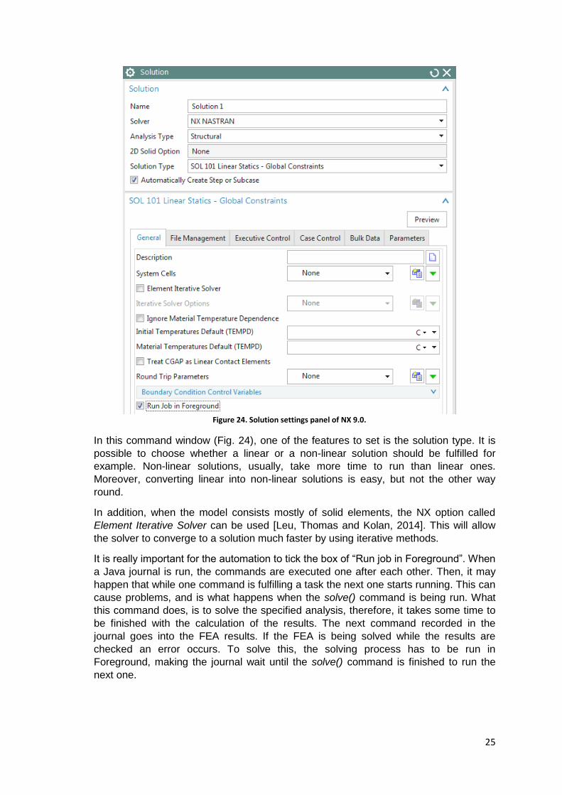
Figure 24. Solution settings panel of NX 9.0.

In this command window (Fig. 24), one of the features to set is the solution type. It is

possible to choose whether a linear or a non-linear solution should be fulfilled for

example. Non-linear solutions, usually, take more time to run than linear ones.

Moreover, converting linear into non-linear solutions is easy, but not the other way

round.

In addition, when the model consists mostly of solid elements, the NX option called

Element Iterative Solver can be used [Leu, Thomas and Kolan, 2014]. This will allow

the solver to converge to a solution much faster by using iterative methods.

It is really important for the automation to tick the box of “Run job in Foreground”. When

a Java journal is run, the commands are executed one after each other. Then, it may

happen that while one command is fulfilling a task the next one starts running. This can

cause problems, and is what happens when the solve() command is being run. What

this command does, is to solve the specified analysis, therefore, it takes some time to

be finished with the calculation of the results. The next command recorded in the

journal goes into the FEA results. If the FEA is being solved while the results are

checked an error occurs. To solve this, the solving process has to be run in

Foreground, making the journal wait until the solve() command is finished to run the

next one.

26

Finally, parameters that affect the solution convergence can be modified, as well as

other settings that are not explained in this thesis as they do not affect to the study

case.

3.1.3. Meshing features

After the geometry is created, comes the meshing part. There are different meshes for each dimensional element and the main tools can follow this classification:

Figure 25. Free mesh and Mapped mesh examples [Ansys, 1998].

Before meshing the model, and even before building the model, it is important to think about whether a free mesh or a mapped mesh (Fig. 25) is appropriate for the analysis. A free mesh has no restrictions in terms of element shapes, and has no specified pattern applied to it. Compared to a free mesh, a mapped mesh is restricted in terms of the element shape it contains and the pattern of the mesh. A mapped area mesh contains either only quadrilateral or only triangular elements, while a mapped volume mesh contains only hexahedron elements. In addition, a mapped mesh typically has a regular pattern, with obvious rows of elements. If you want this type of mesh, you must build the geometry as a series of fairly regular volumes and/or areas that can accept a mapped mesh. These Free and Mapped meshes are strictly related to 2D and 3D meshes and are meaningless for the 1D meshes.

27

Figure 26. Different meshes available in NX 9.0.

As it is shown in the figure above (Fig. 26), all the geometries can be meshed,

independently of their dimension. In the case of this thesis the 1D Mesh takes major

relevance.

Figure 27. 1D Mesh panel of NX 9.0

The panel displayed above (Fig. 27) shows the setting of the chosen 1D Mesh option. The objects of interest are chosen and the selected type of section is defined. There are multiple section types available (Table 1).

28

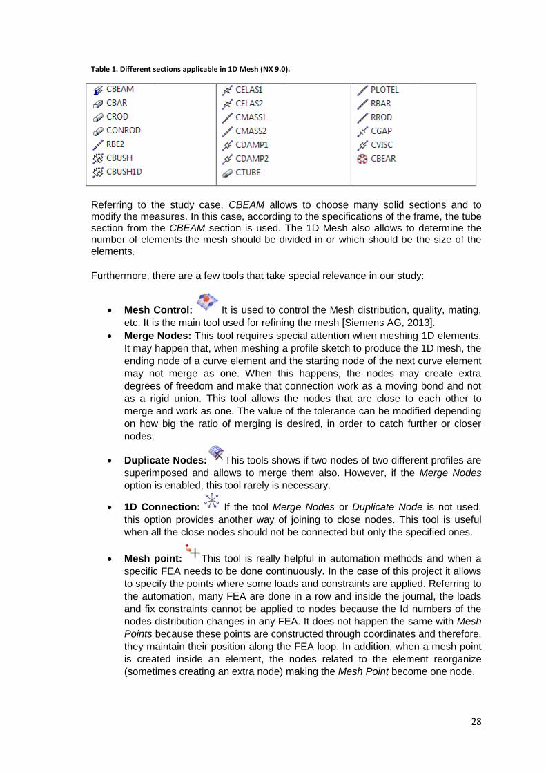
Table 1. Different sections applicable in 1D Mesh (NX 9.0).

Referring to the study case, CBEAM allows to choose many solid sections and to modify the measures. In this case, according to the specifications of the frame, the tube section from the CBEAM section is used. The 1D Mesh also allows to determine the number of elements the mesh should be divided in or which should be the size of the elements.

Furthermore, there are a few tools that take special relevance in our study:

Mesh Control: It is used to control the Mesh distribution, quality, mating,

etc. It is the main tool used for refining the mesh [Siemens AG, 2013].

Merge Nodes: This tool requires special attention when meshing 1D elements.

It may happen that, when meshing a profile sketch to produce the 1D mesh, the

ending node of a curve element and the starting node of the next curve element

may not merge as one. When this happens, the nodes may create extra

degrees of freedom and make that connection work as a moving bond and not

as a rigid union. This tool allows the nodes that are close to each other to

merge and work as one. The value of the tolerance can be modified depending

on how big the ratio of merging is desired, in order to catch further or closer

nodes.

Duplicate Nodes: This tools shows if two nodes of two different profiles are

superimposed and allows to merge them also. However, if the Merge Nodes

option is enabled, this tool rarely is necessary.

1D Connection: If the tool Merge Nodes or Duplicate Node is not used,

this option provides another way of joining to close nodes. This tool is useful

when all the close nodes should not be connected but only the specified ones.

Mesh point: This tool is really helpful in automation methods and when a

specific FEA needs to be done continuously. In the case of this project it allows

to specify the points where some loads and constraints are applied. Referring to

the automation, many FEA are done in a row and inside the journal, the loads

and fix constraints cannot be applied to nodes because the Id numbers of the

nodes distribution changes in any FEA. It does not happen the same with Mesh

Points because these points are constructed through coordinates and therefore,

they maintain their position along the FEA loop. In addition, when a mesh point

is created inside an element, the nodes related to the element reorganize

(sometimes creating an extra node) making the Mesh Point become one node.

29

3.1.4. Different Constraints

NX compresses many ways of applying the boundary conditions. On one side, there

are the Loads which can be used to express all the efforts or reactions the model

suffers (Fig. 28) and on the other side, there are the constraints that fix the different

degrees of freedom (Fig. 29).

From the different loads available the Force is the one used in the experimentation of

this thesis.

Figure 28. Load type panel of NX 9.0.

Figure 29. Constraint type panel of NX 9.0.

The requirements to set a force correctly are, the place where it is applied (i.e. mesh point, surface, edge…), the value of it coherent with the unit and the direction of the force.

Moreover, applying the fix constraints follows the similar method, except there is not a direction needed. There are six degrees of freedom (DOF) that can be fixed. Three that are related to the displacement along the main axes (X, Y, and Z) and other three related to their respective rotations. If the analysis requires not to fix all DOF it is possible to use the tool “User defined constraint”, where you can fix the desired DOF [Leu, Thomas and Kolan, 2014].

3.1.5. Post processing features

Once NX Nastran solves the solution, the results button become available.

Inside the different results are displayed. The results can be divided into two different

solution groups, displacement solutions and stress solution, as it is a structural

analysis.

30

Figure 30. Different results available in NX 9.0.

As shown in the figure above (Fig. 30), on one side, there are the displacement and

rotation solutions. They show how the frame has been deformed and in which direction.

The NX software is able to show the displacement and rotation along every axis, as

well as the whole magnitude.

On the other side, there are the solutions related to the stress that the part suffers.

Through these solutions it is possible to recognize the critical zone of the part and

whether it would break or not. Between the stress solutions available, there is the Von

Mises Stress one. It is useful to study this solution when the frame has a malleable

material applied.

One interesting option during the post-process is to create a report out of the results

obtained. This helps to organize and produce a summary of the whole study and

display all the properties and characteristics of it, as well as the maximum and

minimum values of the different solutions.

The report includes the following features of the FEA:

Introduction

Solution Summary

Materials

Sections

Modeling Objects

User Defined Groups

Meshes

Physical Property Tables

Solution Steps

Loads

Constraints

Solution Objects

Results

Images

3.2. Material database

Nowadays, the material selection takes a major importance in the world of

manufacturing and production. Therefore, FEA software provides a large material

database to study how the structures behave and be able to choose the more suitable

ones. Furthermore, the current technology in material science allows the creation of

new materials with extraordinary properties that create infinite possibilities of

improvement.

31

3.2.1. Type of materials

One of the main characteristic of materials is the different behavior they may have

depending on the direction in which they are tested (Fig. 31) and the physic state in

which they are. Basically, it is possible to divide the material into the four following

subclasses:

Isotropic materials: The properties of the material are independent of the

direction.

Orthotropic materials: The properties of the material are different in their

symmetry (90°) planes.

Anisotropic materials: The properties of the material depend on any direction

(i.e. wood)

Fluid materials: Commonly used in heat transfer and flow analyses. They can

be liquids or gases.

When talking about the properties of the materials, the reference is made for example,

to elasticity, temperature, conductivity, light speed…

Figure 31. Different behavior of materials depending on the direction [Mohite, 2006].

3.2.2. Material categories

The materials, due to its composition, can be classified in different categories:

Ceramic: They are good insulating material. Among their properties it is

appropriate to emphasize their high E-young modulus. Due to their fragility, they

take minor part in the analysis. Fig. 32 shows various examples of pieces of this

material.

Figure 32. Ceramic material (tile) [Montes, 2014].

Metal: Known for their high mechanical resistance (pulling, compression efforts)

and strength, they are really hard materials. They are commonly used in the

engineering industry. Famous examples are iron, steel, aluminum, brass,

copper and lead. Fig. 33 shows various examples of pieces of this material.

32

Figure 33. Metalic objects [WIS, 2014]

Plastic material: They are materials formed by a wide range of synthetic or

semi-synthetic organics that are malleable and can be molded into solid objects

of diverse shapes. The diversity is so high that plastic materials with almost all

ranges of properties can be found. A good example is rubber (Fig. 34).

Figure 34. A car tire [Michelin, 2015].

Polymer: Basically they are macromolecules. It is a material formed by the

union of monomers. As well as the ceramic materials, the polymers do not fit

well for the purpose of the study. Fig. 35 shows various examples.

Figure 35. Plastic envases [Wikipedia, 2015].

Other: Mainly fluid materials: gas, liquid, resins (i.e. epoxy).

3.2.3. Non linearity of materials

In studies such as the one of this thesis, the hypothesis of the limit of elasticity is not

always fulfilled. It can happen that sometimes, the material tested overcome its elastic

limit and breaks the linearity limit point. In order to analyze that large deformation it is

mandatory to know how the material behave in those situations and how it evolves [Gil

Espert, 2011].

This behavior of the material properties can affect enormously to the results of the

tests.

3.2.4. Material library in NX 9.0

33

The Siemens software provides us with a large library of different materials. All of them

are stored in the “UGII” folder of the NX 9.0 directory. In that folder all the properties

and constants related to each material are classified. The default “Physical Material

Library” of NX is formed by 86 materials. Attached in the Appendix can be found the

complete list of materials of the NX library.

In addition to the existing materials, new ones can be added. In order to create a new

material its relevant parameters and property values should be inserted. The main

properties that can define a mechanical material are the following ones:

Mass Density (ρ) (𝑘𝑔

𝑚3⁄ )

Young’s Modulus (E) (MPa)

Poisson’s Ratio (ν) (0..1)

Shear Modulus (G) (MPa)

Structural Damping Coefficient (GE) (optional)

Isotropic, linear and homogenous materials: 𝐺 = 𝐸

2(1+ν)

When the creation of a non-isotropic material is required, the “material property matrix”

should be inserted.

This matrix should be formed by the different expressions that set how the properties

are developed in the different directions.

34

4. IMPLEMENTATION OF AN AUTOMATIC FEM

ANALYSIS

This chapter includes all the explanation of the implementation of the practical case in

detail, taking into account the basic facts from the previous chapters.

4.1. Goals and concept of the implementation

A decision support assistant for sustainable product development is conceived and

implemented in the course of the project SFB 1026 sustainable manufacturing. One

use case for the assistant system is the automatic identification of sustainable options

for a given product under given restrictions.

This thesis will contribute to this solution by implementing an automatic FEM analysis

to verify that the frame met the strength requirements. The automatic analysis allows

for analyzing multiple options in a timely manner and it is based on NX Open. The

solution is designed and tested based on the example of a pedelec frame. The different

materials for the pedelec frame are tested and the suitable ones are automatically

identified. The thesis will further be a base for analyzing different parameters such as

the geometrical ones.

4.1.1. Procedure of the implementation

The automation is formed by different parts that, when they are together, make the

whole process possible and successful. Following, the different characteristics are

explained in detail and why their tasks are necessary.

4.1.1.1. External connection Eclipse-NX

One of the first conditions that the automation requires, is that it should be able to be

run from outside NX. The programming chosen language is Java and the surface used

to edit and test the Java files is Eclipse. Eclipse provides the essential tools to edit and

create any file from the Java environment.

The connection between the Session from NX and the Java files in Eclipse happen

thanks to the Licensing Example from the NX Open interface, included in the NX Java

Examples folder from UGII directory. The aim of this example is to show how to sign a

jar file and the caveats with running the jar file. Formed by four java files, it allows

running a recorded Java journal from Eclipse platform, outside of NX.

Before running the Licensing example, it is mandatory to save and compile all the files

related to the main one and start a session on NX. Once done these steps, it is allowed

to run the main java file which would run all the process.

This implementation of java files being run from outside NX works as a basis for the

correct development of the automation.

Sometimes, it may happen that the NX Open libraries are not related to the Java

workspace. That may happen if the workspace is changed of directory or if some

software is reinstalled. This easily fixable, adding to the environmental variable of the

system “PATH” the root to the missing library.

35

4.1.1.2. Inclusion of Journals

The Journals take a major importance in this project. The Journal capability of NX is an

automation tool that records, edits and replays the sessions performed by the user. Via

the session of NX, it produces a scripted file which can be run later to replay the

session. The produced file can be easily edited with simple programming constructs

and user interface components to create rapidly generated customized programs

[Siemens AG, 2010].

In the case of this project, the journal attached in the Framejournal.java file, contains all

the commands that would affect the frame automation. The journal target is, mainly,

fulfilling an FEM analysis with the frame applying each material and saving the

simulation file which also is analyzed and contains the solution values that are

compared to determine the optimum material according to the parameter of studying.

Finally, during the journal, it is set that the model is loaded, the FEM and simulation

files created and, at the end the simulation file is saved. However, when the automation

wants to be implemented in another workplace the directory should be changed. For an

easy fix of this issue, the code lines where the directories should be change, are

provided in the Appendix 3.

4.1.1.3. Access to the material library

In order to observe which method was used and how to assign the material to the

body, a Journal was recorded with the only proposal of assigning a single material to

the body. When checking the Journal, it shows that the material is load from the

material library and assigned to the bodies with the following method:

workFemPart.materialManager().physicalMaterials().loadFromNxmatmllibrary("St

eel")

In this case the Steel material is applied to the FEM part of the model.

The method shows that it loads the material from the NX material library and the

argument it needs is the string name of the material. However, as it is a process

automation, and it needs to load different materials, a way to access to those string

names is needed.

4.1.1.4. Extracting elements from XML file (Parsing)

Inside the NX directory files, there is a folder exclusively related to the materials and

their libraries. One of those file is the physicalmateriallibrary file. It is an XML

(Extensible Markup Language) file and inside, there are stored all the materials and

their properties and characteristics. The XML files are frequently used to classify

different kind of libraries [Pieterse, 2011] and provide some advantages:

They have a structured and described format.

Their data is hierarchically organized. There are relationships between data.

Their format is discoverable, parsing and standard. It can be read by

Microsoft Excel and extract the different nodes.

As mentioned, the XML files store its data in a hierarchical structure where each

element (better called node) represents a piece of information of the materials (i.e.

name, category, Young Modulus, etc.).

36

This structure of the file helps in a great amount in order to extract what really matters,

the string name. A way of programming the “extraction” of the name node, is by, what it

is called inside Java, parsing. Through programming the Parser method the program

reads an XML file and takes, in this case, the element related to Name of each material

and converts it into an string [Naughton and Schildt, 1999].

This extraction of nodes happen in the DomParserExample.java file, where the XML

file is parsed. Inside this file too, there is a command which loads the material library

file and is located in the line code 59 of the file.

As it will be explained later, not only the string name is extracted, also the value related

to the “Yield_14” tag name which makes reference to the Yield Strength value of the

material.

4.1.1.5. Creation of Material Loop

Once it is known how to get the string name reference of the material, the next step is

to enable the Journal to proceed executing its commands material by material, one by

one. That is possible by storing all the material string names in one list and executing a

loop through it.

Enabling again the Parser Method feature, it allows extracting the strings related to the

Name element from each material and storing them in an ArrayLIst. This way, all the

journal can be executed inside a loop designed with the for structure [Liguori R. and

Liguori P., 2015], that runs the programs along all the list, working each time with one

material.

4.1.1.6. Obtaining critic nodal values

A main part of the automation consists in taking a decision about the more suitable

material automatically.

After the FEM analysis is performed with the selected materials from the NX library, the

different solutions related to the structural analysis are displayed.

A good way to choose a right material is by a comparison of the most critical nodal

values of each simulation. During the post-process, using the NX tool “Result

Measure”, it is possible to extract a critic nodal value. During the loop, is possible to

add this value to the material related to it. In this way, the material element list created

before, which only contains the material names, would contain the nodal magnitude

too.

Furthermore, with the “Result Measure” tool it is possible to store more than one value.

In this case, as it will be explained later, the highest nodal strain and stress are stored

for the automation.

Inside the journal, two values are stored in an Array that is returned later to use their

values for fulfilling the conditions explained later. The two values stored are double

values, and make reference to the maximum nodal displacement and stress.

4.1.1.7. Comparison of the results

At this point, a list is designed, whose positions contains the material name and the

nodal maximum magnitude of stress and strain.

37

In order to set that the tested one is an appropriate material, its stored value should

fulfill a condition. This condition would be a value that every successful material should

achieve.

Depending on the parameter analyzing the condition has different requirements:

For the strength condition, the Yield Strength value is more relevant. This value

is defined in engineering and materials science as the stress at which a material

deform plastically. As the load applied to the model increases the model can

pass from the elastic zone to the plastic one. If the stress suffered does not

overtake this yield limit, the model deforms but can recover its original shape.

However if the load is higher the model can enter the plastic zone where it

suffers a bigger deformation without being able to recover its original form.

When a yield point is not easily defined based on the shape of the stress-strain

curve an offset yield point is arbitrarily defined. The value for this is usually set

at 0.1 or 0.2 % plastic strain [Callister and Rethwisch, 2005].

For guaranteeing that the material does nor deform plastically or break, a safety

factor is taken into account. This safety factor is determined by the FEM

analysis characteristics. Taking into account the forces implemented in the

FEM, a safety factor of the 0.8 of the yield strength is reasonable.

To sum up, the first condition requires that the highest stress value obtained

from the FEA cannot be higher than the 80 % of the yield point value of each

material.

However, the stress of a model is dependent of the forces and geometry

specifications therefore, the maximum stress values are the same for the model

tested with every material.

Then, a second condition needs to be implemented. In order to choose

materials that can provide stiffness to the model, a maximum deformation limit

has been set. The maximum deformation value cannot overcome 1,5 mm. This

limit has been chosen taking into account the overall dimension of the model

and how this displacement can affect to the correct operating of the frame

without causing any problem.

Finally the two conditions are summarized:

1. Max. Stress < 0,8 x Yield Strength (kPa = mN/mm2)

2. Max Strain < 1,5 (mm)

4.1.2. Selection of materials

The material library provided by NX 9.0 contains 86 materials. The materials are really

different between them and making the automation through all the materials lacks of

much sense due to its extra calculus time that is wasted. In order to optimize the

automation and make it faster, some of the materials from the library have been

removed following diverse criteria. In the next points, those selections are explained.

4.1.2.1. First selection

The execution of the FEM analysis to each material is not fast, as the frame is formed

by several parts that should be meshed one by one containing many elements. Within

a fast look to the NX material library, it is possible to detect some materials that are

physically impossible to fit the frame. Those materials appear in the library comprise

38

inside the Others called Class and are mainly fluids (liquids, gases and resins).

Summarizing, from the 86 available materials the following ones can be rejected:

Acetylene C2H2 Gas/Liquid

Air

Ammonia Gas/Liquid

Argon Gas

Bismuth Liquid

Carbon Dioxide Gas/Liquid

Engine Oil Liquid

Epoxy

Ethylene Glycol Liquid

Freon Liquid R12

Glycerin Liquid

Helium Gas

Hydrogen Gas

Isobutane Gas/Liquid

Lead Liquid

Mercury Liquid

Methane Gas

Methanol

Nak Liquid (22-78/45-55)

Nitrogen Gas

Oxygen Gas

PbBi Liquid

Potassium Liquid

Propane Gas

R134a Gas/Liquid

Sodium Liquid

Sulfur Dioxide Liquid

Water saturated liquid/ vapor gas

Those 37 materials ease the process to safe a great amount of time and avoids the

generation of useless data. After the first material selection, the library reduces until 49

materials.

4.1.2.2. Second selection

One aim of the material requirement is to be isotropic. In other words, all the properties

of the material should behave equal in any direction, otherwise the behavior of the

frame becomes unpredictable. For example, if the frame is made of wood, the

simulation would not be accurate because the wood has anisotropy and, as the design

of the model covers the different axial directions is not possible to analyze how it can

behave under the loads. The bonds of the the frame would not show realistic results as

the wood respond differently to loads apply in the direction of the fibers or the ones

applied perpendicularly to them

Inside the material library there are artificial materials created with anisotropic and

orthotropic properties. As they are not useful in our study, they can be also rejected.

The materials are the following ones:

39

Aniso Sample

Ortho Sample

Ortho Sample Legacy

Ortho Sample W Damping

Rejecting these 4 materials helps to produce a more efficient loop as the material

library contains only 45 materials (metals and plastics), almost half of the initial number

of materials displayed.

4.1.2.3. Third selection

As a reference for the strength condition, the yield strength coefficient is taken,

however, depending on the chosen material, this coefficient is not constant. After

analyzing thoroughly the updated material library, it is observed that some metals and

plastics have not this property as a constant value. The temperature can influence the

Yield Strength constant and the materials that are more likely to vary this coefficient

have it tabulated inside the NX material library. During the analysis, the temperature

increment that the frame has is not taken into account. Because of that the following

materials are not taken into account for testing:

AISI 310 SS

AISI 410 SS

Aluminum 2014

Aluminum 6061

Polyurethane Soft

S/Steel PH15 5

Steel

Titanium Alloy

Waspaloy

The library contains 36 solid materials that have a constant Yield Strength coefficient

and isotropic properties.

4.1.2.4. Final material library

Finally, the initial material library from NX has been reduced from 86 to 36 materials.

The materials included on it are metals or plastics, all of them in solid state. Also, they

have isotropic properties and their Yield Strength value remains constant for the

analysis. These 36 materials are the ones that are tried in the automation and FEA is

performed to the frame with each one.

These are the materials:

ABS

ABS GF

Acrylic

AISI SS 304

AISI Steel 1005

AISI Steel 1008 HR

AISI Steel 4340

Aluminum 5086

Aluminum A356

40

ASI Steel Maraging

Brass

Bronze

Copper C10100

Inconel 718 Aged

Iron 40

Iron 60

Iron Cast G25

Iron Cast G40

Iron Cast G60

Iron Malleable

Iron Nodular

Magnesium Cast

Manten

Nylon

Polycarbonate

Polycarbonate GF

Polyethylene

Polypropylene GF

Polypropylene

Polyurethane hard

PVC

SMC

Steel Rolled

Titanium Annealed

Titanium Ti 6Al 4V

Tungsten

4.1.3. Geometrical restrictions and final model

In first instance, the model used for implementing the automation was the front side of

the Smart Tripelec frame designed by NX software (Fig. 36). The different parts of the

3D frame have been designed independently and then joined together forming the final

assembly.

41

Figure 36. Master model of the original Tripelec frame.

However, the given model has a complex geometry which includes many sharp edges

that can affect negatively the FEM analysis by creating Stress singularities.

Singularities: All components have finite radii at corners, nevertheless for

small radii a common simplification is to ignore the radius and make the corner

“sharp”. This may not matter for an external corner; however, a sharp re-entrant

corner results in a stress singularity.

Refining the FEA mesh gives increasing stress values as the element size is

reduced (Fig. 37). The stress results are meaningless (the displacement results

may be acceptable) and a reasonable approximation of the radius must be used

in the model. One way of reducing this problem is to model the component with

a material which can model plastic deformation; however strain at the sharp re-

entrant corner remains infinite. If stresses are not of interest, for example if

modal frequencies are being computed, then the inclusion of a sharp re-entrant

corner will not affect the results and the simplification will help to simplify the

model [Reiner and Binde, 2014].

42

Figure 37. Variation of singularities [Reiner and Binde, 2014].

During the study process, the model specifications have encountered several problems

that have made the procedure to modify and adapt to the circumstances at any time.

On one side, the geometry of the model has been limited in a certain way due to its

sharp edges and complex high data consuming design. The edges make a big effect in

the study because they may create the singularities mentioned before. At the same

time these singularities may cause “pick values” that can alter strongly the results of

the automation.

Therefore, the decision to model the frame with 1D elements seemed to be a fair

option. The frame conserves the constant tubular sections of it and adapts those parts

where the section varies but not significantly.

Choosing the 1D model, brings some advantages compared to the original 3D one:

First, the calculus time used by the solver decreases drastically as the 1D

model contains less nodes and its mesh is formed by less elements.

43

In addition, the results of a 1D model for this type of studies (static linear) are

better than the ones from 2D or 3D. That is because the result value of each

element is calculated taking into account the results of the elements right next

to it and, therefore, the error in the element calculus can be accumulated from

element to element. Then it is easy to realize that a model with less elements

makes this accumulative error smaller.

Referring to the chosen 1D elements, mostly beams, for solving them there are two

main principles used: Bernoulli and Timoshenko:

On one side, Bernoulli is more accurate for thin and long bars and it does not

take into account the Shear Modulus (G). Therefore, it is consider as an

efficient method of calculation.

On the other side, Timoshenko is preferable for shorter bars and it takes the

Shear into account. For that, it calculates the results using the “Shear factors”

and therefore, the geometry of the section is considered. Among the

geometries of the section, the results are more reliable for constants sections

such as a rectangular one.

Referring to the use of 2D elements, they are useful when the model has an overall

constant thickness (i.e. wine bottle). Then it can be meshed by mid-surfaces and apply

the thickness.

Finally, the 3D analysis should be avoid as they can give less accurate results. That

lack of efficiency is created because the 3D elements need to fit between them and

making the nodes of the edges coincident carries a bigger effort.

As a result, the main reference first geometry is refused due to its geometry complexity

and the constraints problems it can give. Then, the next selection includes, mainly, the

center main part of the frame (Fig. 38).

Figure 38. Model of the central frame in 3D.

Finally, it is easily observable that the central part of the frame (Fig. 38) can be

approximated to a 1D element (beam type). The model of the 1D element (Fig. 39) is

defined by drawing the profile line of the frame that can be represented by the axes of

the different tubes connected. Special care was taken in creating a small rounding

between every lines connection. This avoids the creation of singularities and makes the

results display more smooth and realistic.

44

Figure 39. Sketch of the central frame in 1D.

The final model (Fig. 40) consists in 4 sketches formed by profile lines that later are

displayed as 1D elements with their different tubular sections (Fig. 41).

Figure 40. Model of the whole final frame in 1D.

45

Figure 41. Model of the final frame with the mesh applied.

The first profile line (Fig. 42) is the central main part and has been designed following

the measures of the master model, the unions between lines are rounded with a radius

of 50mm and the section added to it is tubular with an inner radius of 23 mm and outer

radius of 25 mm.

Figure 42. First sketch.

The second sketch (Fig. 43), shows the horizontal bars where the seat goes attached.

As well as the first sketch, the measures are taken from the master part, the unions are

rounded and the tubular section added has an inner radius of 7 mm and outer radius of

8 mm.

46

Figure 43. Second sketch.

The third sketch (Fig. 44) has the same section as the second one and represent the

bars connected to the main frame that help distributing the efforts caused by the use.

Figure 44. Third sketch.

The fourth and last sketch (Fig. 45), consist in the transversal top bar of the frame that

connects with the back wheel bonds. Also, the measures are taken from the master

model and its section is tubular as well, with an inner radius of 15,5 mm and outer

radius of 17,5 mm.

47

Figure 45. Fourth sketch.

Once the geometry is created, there are some bonds from the back and front wheels

that have been simplified in our 1D model and have been marked with the Mesh Point

tool. There are five mesh points in total and the coordinates are the following ones:

Attached on the appendix it is shown the drawings of the frame with the measures.

4.1.4. Characteristics and restrictions of the FEM analysis

After the model of study is completely defined, it is possible to proceed with the FEM

analysis.

First, the model is meshed in accordance with the specified requirements and better

mesh criteria.

After, the loads and the fix constraints the model suffer are applied. As it can be

appreciated in the pictures, the bonds between the frame and the wheels (back and

front ones) and pedal are the most important ones for the study, as well as the two bars

where the seat is attached.

4.1.4.1. Meshing

As it has been explained before, the 1D Mesh tool is used to mesh the different

sketches. With this tool the objects to mesh are selected and the dimensions of the

frame are specified, as well as the material related to it. Other important aspect to

decide is the Element size of the mesh.

In order to know if the FEA is reliable, different tries of the FEA have been done,

changing the element size at a time. With this test, on one side, it is possible to confirm

that the results of the different FEA are useful, and on the other side, it helps to decide

the element size used in the automation.

48

Figure 46. Result plot with 100 mm element size.

Figure 47. Result plot with 50 mm element size.

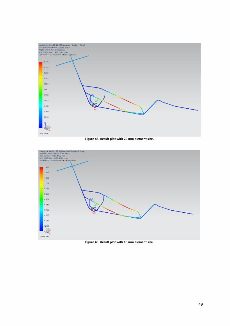
49

Figure 48. Result plot with 20 mm element size.

Figure 49. Result plot with 10 mm element size.

50

Figure 50. Result plot with 5 mm element size.

Figure 51. Result plot with 2 mm element size.

The six deformation result displays shown above (Figures 46-51) refer to six FEA

tested with different mesh element sizes (100 mm, 50 mm, 20 mm, 10 mm, 5 mm, 2

mm). In this case the material applied is “AISI SS 304” and the loads and constraints

applied are the ones of the current implementation that are specified in the next

subchapters.

Taking a look at the result values, the maximum strain values do not differ much from

the biggest to the smallest elements. In element size decreasing order the maximum

nodal deformations are: 1,404 mm; 1,464 mm; 1,476 mm; 1,478 mm; 1,480 mm; 1,480

mm. The percentage variation from the lowest (100 mm) and the highest (2 and 5 mm)

values is 5,14 % and the variation from the second lowest (50 mm) and the highest is

of 1,08%. As the values are almost identical, it is possible to conclude that the FEA is

reliable.

51

For choosing the element size of the mesh, 10 mm has been the option because it is

when the result value shows that is stabilized and barely change anymore when

reducing the element size (+/- 0,002 mm). It is a good size and it the amount of effort

required from the solver is not high as the solution file is about 11 Mb.

4.1.4.2. Forces

First of all, it is necessary to be aware that among the world population, each user

physical properties (weight, height, strength…) are different. Therefore, the FEM

analysis should cover the majority of the users’ capabilities. In other words, the

analysis should be adapted and performed to a frame that is able to support the

majority of most unfavorable cases.

The forces that are applied are basically the weight of the user and the reactions

suffered in the wheel bonds because of the effort made by the user pedaling.

On the back wheels bonds there are two facts to take into account: First, the reaction

the suspension does from the back wheel to the mid bond and the direct effort that the

frame supports from the each wheel both in the upper and down bond. The effort of the

suspension is in the same direction of it, 45° respect the XY plane. The wheels make

the force directly vertical in contact with the floor and its answer effort is distributed

between the down and upper bonds also in vertical (axis Z) direction. Figures 52-54

show the back part of the frame and how the loads are displayed.

Figure 52. Master model.

Figure 53. Solid mesh.

Figure 54. Curves mesh.

In the middle part of the frame, as it shown, the seat goes attached to the two thinner

bars. Here is where the user seats and therefore the two bars are the ones that

transmit the weight of the user vertically. As the user is in pedaling position, there is

and effort applied backwards in the seat. . Figures 55-57 show the middle part of the

frame and how the loads are displayed.

Figure 55. Master model.

Figure 56. Solid mesh.

Figure 57. Curves mesh.

Finally, the forces applied to the front side of the frame are only the ones related to the

front wheel. The reaction is applied on the ending bar of the model perpendicularly

respect the line in the XZ plane. . Figures 58-60 show the front part of the frame and

how the loads are displayed.

52

Figure 58. Master model.

Figure 59. Solid mesh.

Figure 60. Curves mesh.

Once the direction of the forces is designed, the values that each one should have is

determined. The values should be coherent with the balance of the analysis and be

realistic taking into account the unfavorable cases mentioned before. Then, after

studying the complexion of the general user model a weight of 100 kg has been

chosen. This value covers the major population and is suitable for our study.

The weight of 100 kg is transformed to N using a rounded gravity acceleration value of

10 m/s2.

The two seating bars share the 1000 N of the weight, 500 N on each, and also 100 N

backwards in the X direction due to the effort back from the pedals.

The weight effort is answered by the front and the back wheels. As the user is laying

back in his seat his position of the user is more close to the back wheels than the front

one therefore the back wheels cover the 80% of the weight and the front one 20%.

That percentage of 20 % is fully applied to the front one upwards however the reaction

is not totally vertical due to the bond so the force split in 200 N in Z direction upwards

and 50 in the X direction backwards.

The distribution of efforts in the back wheels is a bit more complicated. The 80 % of the

weight is distributed in three bonds or unions and the upper bond follows also the

symmetrical distribution dividing that amount in two for each wheel. Therefore, the

effort values do not differ much in each bond. The lowest bond suffers 250 N in upper

vertical direction, the suspension bond reflects its reaction with a 45° respect de XY

plane and split in 250 N in both X and Z positive directions, and last the upper bond

suffers 300 N in upper direction but divided into the both extremes of the transversal

bar, therefore, 150 N in each extreme in vertical Z direction.

Below, the final disposure of the loads is shown (Fig. 61).

53

Figure 61. Final appearance of the applied loads.

4.1.4.3. Fixed Constrains

After the loads are applied the next step is to restrict the movement of specific parts of

the frame according to realistic behavior. In order to know which parts of the model fix

and which degrees of freedom, it is important to predict the movement of the model, in

other words, the behavior of the model under the applied loads.

A successful FEA is done only if the model is fix in some point and does not allow to

rotate or translate indefinitely in any direction.

As far as the movement of a bike is known, the wheels of the bike are in permanent

contact with the ground and that is the reason why the bonds between the wheel and

the frame should be fixed in vertical direction (Z axis) (Fig. 62). However, in the model

used, the bonds related to the back wheels are not directly connected to them, in

addition, there is a bar that connects the back wheel and the bonds of this FEA. As a

consequence, only the front wheel is fixed vertically. A mesh point is used to indicate

the last point of the frame where the bond is.

Figure 62. Fixed constraint of the front wheel.

A vertical fixation is not enough to proceed to solving and the bottom curve from the

central structure has been fixed in all DOF. This decision has been taken after making

a global balance of the forces and analyzing the possible behavior of the frame. Fixing

54

that small frame curve (Fig. 63) allows to visualize better the deformations of the frame

and clarifies where the reference is.

Figure 63. Fixed constraint of the bottom curve.

Finally, none of the rotations (x,y,z axis) have been fixed to allow the body to perform

these possible movements as the analysis is not symmetrical in any plane.

4.2. Calculus time of the results

One important aspect of the implementation is observing the running time the program

needs to perform the loop of FEM analysis.

If the FEA is performed manually in NX, after the solving the FEA apart from the FEM,

SIM and PART files there are more files generated. One of these is the “.log” file. This

file contains information about how the solver has worked and all the process are

organized chronologically displaying the calculus time needed by the solver.

Apart from that, it is important not to forget that the time a solver takes to fulfill its works

varies a lot.

One of the main aspects is the computational time and it differs from the CPU used in

each case. For example, an ordinary laptop does not take the same time to perform the

same FEA than a computer from NASA.

Another aspect to take care is how the journal is recorded. When recording a journal,

all the commands that alter the Session are recorded. For example, if the user zooms

in and zooms out to see the model those “movements” are recorded into journal. It is

important to optimize the journal and delete useless code lines. As it is an automation,

the more useless commands from the journal are deleted, the faster it will take the loop

to run.

In the case of the automation, the time has been measured before and after the loop.

The test has been tried in a laptop HP Pavilion dv6 Notebook PC with a processor Intel

Core i7 – 2630QM CPU of 2.00 GHz.

As it was displayed, the automation took 284 seconds (4:44 min) for performing the

FEA for the 36 materials. Almost all the FEA last between 7 and 8 seconds, except the

first one that takes a bit longer (15 seconds) due to initialization processes.

As mentioned above, this time measure can be influenced by many factors such as the

capacity of the processor, the optimization of the coding and the complexity of the

analysis

55

5. CONCLUSION

After testing the implementation, the results are exposed and it is time to proceed to

their interpretation.

5.1. Interpretation and study of the obtained results.

The sustainable option to measure is the Strength. The Strength defines how much

load the frame can suffer without suffering a large deformation (in relation to its original

dimensions) or breaking (depending on the chosen material).

The analysis results show two different solution groups, displacement solutions and

stress solution, as it is a structural analysis. However, talking about the results, there

are some results more trustworthy than others.

The first calculation that the solver does is the deviation of the nodes. From the

deviation, the strain results are calculated. And finally, from the strain, the stress results

are calculated. That means that along the different steps of the chain there is a

calculation error that is accumulated. Therefore, the strain values are more reliable

than the stress ones.

Referring to our automation the frame with the material tested needs to fulfill to

conditions. The first one says that the maximum stress suffered by the frame (equal for

all materials) needs to be lower than the 80 % of the yield strength of the material.

Looking at the automation results, the FEA maximum stress value is of 59,64 MPa

(59640 kPa). The materials that fulfill this condition are 24 out of the 36 available,

therefore, there are 12 materials not suitable for the frame. These materials are

basically plastics and are here listed:

ABS

ABS GF

Acrylic

Copper C10100

Nylon

Polycarbonate

Polycarbonate GF

Polyethylene

Polypropylene

Polypropylene GF

PVC

SMC

All of them are plastics except the copper. Usually, these type of plastics tend to be

easily deformable. They can resist small loads without problems but they are not

suitable for producing a bike frame.

However, the suitable materials are still not decided as there is a second condition the

frame should achieve. The maximum deformation of the frame should not exceed the

1,5 mm.

During the loop, in the information prompt of Eclipse the different nodal maximum

magnitudes related to the material, appear. At the same time the different materials

56

that fulfill the two conditions are stored into a new list. Finally at the end of the

automation, a list is provided including the materials suitable for the frame.

In the case of our frame automation, the materials that also fulfill the deformation

condition are:

AISI SS 304 Annealed Max. deformation magnitude = 1,4784 mm

AISI Steel 1005 Max. deformation magnitude = 1,4017 mm

AISI Steel 1008 HR Max. deformation magnitude = 1,3543 mm

AISI Steel 4340 Max. deformation magnitude = 1,4545 mm

Inconel 718 Aged Max. deformation magnitude = 1,3761 mm

Manten Max. deformation magnitude = 1,3783 mm

Steel Rolled Max. deformation magnitude = 1,3636 mm

Tungsten Max. deformation magnitude = 0,7017 mm

These 8 materials successfully fit strength conditions, showing at the same time a

reliable stiffness.

As a final observation, the suitable materials are metals, commonly known for their high

strength and stiffness but some of them also for being heavy.

One material that projects among the other is the Tungsten, this material (Fig. 64)

suffers almost a 50% less deformation than the other suitable materials.

Figure 64. Tungsten [Wikipedia, 2015].

There are a few feature that make the tungsten have that stiffness and properties:

It has the highest melting point of all the elements (3422 °C) and tensile

strength (980 MPa).

It has a high density (19,3 times the density of the water).

The Young Modulus (400 GPa) and Yield Strength (750 MPa) are high

compared to other metals.

However, it has weak grain boundaries, in other words, the interface between

two grains is not strong and disrupts the motion of dislocations through a

material.That is what makes tungsten hard to work with.

Below, it is shown the colored contour plots of the simulation file of the tungsten

applied to the frame.

57

Figure 65. Nodal deformation plot of the tungsten frame.

This plot (Fig. 65) refers to the nodal displacement plot. As It is observable the highest

deformation occurs on the seating bars due to the weight of the user. The displacement

is really small that the undeformed model is not relevant as visually is over superposes

the plot.

Figure 66. Stress result plot of the tungsten frame.

This plot (Fig. 66), shows the Stress results. The parts that more suffer the reaction of

the loads are the bars where the seat is attached but specially the two bars that

connect the sitting bars with the central frame. That happens because the major part of

the load is related to the weight of the user and the load is only distributed through the

sitting bars. Therefore, all the weight load needs to be supported by the bars under the

seat making the mentioned ones suffer the highest values (59,6a MPa).

As a final interpretation of the results, only metal materials have been able to suit the

frame following the strength and stiffness criteria. However, that the material fulfill this

58

condition do not mean they are suitable for the frame production. There are more

parameters that affect the sustainable production of the frame.

Finally, add that during this implementation the material library used was the one

provided by NX 9.0 and it contained a relatively low number of materials. If a more

precise and complete study needs to be fulfilled, new material libraries can be used.

Nowadays, the big manufacturing companies use giant material libraries that contain

thousands of materials. In addition, thanks to the actual technology, more materials are

being discovered or invented, providing a bright future full of possibilities for the coming

engineering projects.

5.2. Outlook

Thanks to the automation implemented, it has been possible to decide automatically

which the strongest materials for a specific bike frame were and in which order and

which materials would deform or break in the same cases.

However, there are more parameters to be studied such as environmental ones (CO2

emissions), weight ones (mass) or economic ones (cost). Therefore, it can happen

also, for example, that the most suitable material for the strength is the most expensive

one or contains a hazardous substance. The more appropriate material for the frame is

chosen only when all the conditions of the parameters that affect the sustainability are

fulfilled correctly.

If a more complete material library is provided, and the conditions of the parameters

adapted to the analysis, it is possible to find optimized solutions for different and more

complex models.

In order to adapt the implementation for testing a further case, it is only necessary to manage some changes related to the implementation. On one side, the specific journal related to the purpose of the study will need to be recorded only once storing the results. For example, if the study consists in how the frame behave under high temperatures, a journal of a thermal FEA must be recorded. On the other side, if additional parameters shall be included into the study, respective conditions must be modified or inserted. For example, for the thermal study mentioned before, the highest temperatures that the frame suffers cannot be higher than the melting point of the material. Those two changes in the implementation allow the study of different parameters that, combined together, will be useful to choose an overall suitable material.

59

REFERENCES

Bibliographic references

Callister, William D; Rethwisch, David G (2005), Materials Science and

Engineering (8th ed.), United States of America: John Wiley & Sons,

p. 164, ISBN 978-0-470-50586-1

Liguori, Robert; Liguori, Patricia (2015), Java: kurz & gut. Java 8 pocket guide

(8th ed.), Beijing: O’Reilly, p. 68, ISBN 978-3-95561-758-5

Naughton, Patrick; Schildt, Herbert (1999), The Complete Reference Java 2

(3rd ed.), United States of America: Osborne/McGraw-Hill, p. 102, ISBN 0-07-

211976-4

Reiner, Anderl; Binde, Peter (2014), Simulations with NX (1st ed.), Munich: Carl

HanserVerlag, p. 86, 215, ISBN 978-1-56990-479-4

Online resources

Allen Jose George, 2012. Ansys vx NX Nastran. [online]. Available at:

http://de.scribd.com/doc/97705562/Ansys-vs-NX-Nastran#scribd [Accessed 6th

June 2015]

Ansys, 1998. How to mesh your solid model. [online]. Available at:

http://mostreal.sk/html/guide_55/g-mod/GMOD7.htm [Accessed 25th July]

Ascon, 2015. APM FEM Add-in. [online]. Available at:

http://ascon.net/solutions/addons/apm/ [Accessed 25th July]

Broekaart, Dolf, 2015. Why should you consider performing nonlinear finite

element analysis?. [online]. Available at: http://www.simuleon.nl/why-should-

you-consider-performing-non-linear-finite-element-analysis/ [Accessed 10th

August 2015]

Burhop, Mark, 2012. NX CAE Tips & Tricks. [online]. Available at:

http://blog.industrysoftware.automation.siemens.com/blog/2012/04/03/nx-cae-

tips-tricks-fea-workflow-part-1/ [Accessed 8th June 2015]

CAE Associates, 2015. Thermal analysis services [online]. Available at:

https://caeai.com/engineering-consulting/fea-services/thermal-analysis-services

[Accessed 5th August 2015]

Cyprien, 2013. FEA Basics – plate with a hole analysis. [online]. Available at:

http://feaforall.com/2013/04/13/fea-basics-plate-with-a-hole-analysis/ [Accessed

10th August 2015]

Dr A Chawla, Finite element method (fem): an overview. [online]. Available at:

http://web.iitd.ac.in/~achawla/public_html/429/fem/overview.pdf [Accessed 18th

June 2015]

Gil Espert, Lluís, 2011. Anàlisis de sensibilidad con comportamiento no lineal

del material y su aplicación en el diseño asistido de estructuras. [online].

Available at:

60

http://www.tdx.cat/bitstream/handle/10803/6862/06Lge06de13.pdf?sequence=7

[Accessed 6th June 2015]

Jan Karel Pieterse, 2011. Characteristics of XML. [online]. Available at:

http://www.jkp-ads.com/Articles/XMLAndExcel02.asp [Accessed 15th July

2015]

M. C. Leu, A. Thomas, and K. Kolan, 2014. NX9 for Engineering Design. [online]. Available at: https://web.mst.edu/~mleu/NX9.0%20Manual.pdf [Accessed 5th May 2015]

Markowitz, Adam; 2012. Finite element modeling (fem) in ansys. [online].

Available at: https://portfolium.com/entry/finite-element-modeling-fem-in-ansys

[Accessed 25th July]

Martínez, Armando; 2009. Los grupos de rotación I. [online]. Available at: http://la-mecanica-cuantica.blogspot.com.es/2009/08/los-grupos-de-rotacion-

i.html [Accessed 18th June]

Montes, Yeisy; 2014. Materiales de construcción. [online]. Available at:

http://yeisimontez.blogspot.com.es/2014/09/materiales-de-construccion.html

[Accessed 25th July]

Morris, Randy, 2008. Mesh refinement. [online]. Available at:

https://cubit.sandia.gov/public/14.0/help_manual/WebHelp/mesh_generation/m

esh_modification/mesh_refinement.htm [Accessed 20th May 2015]

P. M. Mohite, 2006. Lamina constitutives relations in global coordinates.

[online]. Available at: http://nptel.ac.in/courses/101104010/lecture14/14_7.htm

[Accessed 25th July]

Peak, R. S.; Fulton, R. E.; Nishigaki, I.; Okamoto, N.; 1995. A Prototype

Engineering Framework with Graph-based Tool Agents. [online]. Available at:

http://eislab.gatech.edu/pubs/web/mra-overview/efw-framework.html [Accessed

4th June]

Proto3000 Inc, 2013. Finite element analysis services. [online]. Available at:

http://proto3000.com/finite-element-analysis-services-overview.php [Accessed

25th July]

Resolve Engineering Group, 2013. Ship structural analysis. [online]. Available

at: http://www.resolveengineeringgroup.com/ship_structure_analysis.php

[Accessed 25th July]

Roensch, Steve, 2013. FINITE ELEMENT ANALYSIS: Pre-processing. [online].

Available at: http://www.finiteelement.com/feawhite2.html [Accessed 10th May

2015]

Siemens AC, 2013. NX 9 Help. [online]. Available at:

http://www.me.rochester.edu/courses/ME204/nx_help/index.html#uid:index

[Accessed 6th July 2015]

Siemens AG, 2010.NX Programming and Customization. [online]. Available at:

http://m.plm.automation.siemens.com/en_us/Images/4988_tcm1224-4564.pdf

[Accessed 27th April 2015]

61

Siemens AG, 2013. What’s new in NX 9?. [online]. Available at:

http://adacomputers.ro/web/upload/img_fck/Siemens-PLM-NX-Whats-New-in-9-

fs-Y12.pdf [Accessed 27th July 2015]

Siemens AG, 2015. Structural Analysis. [online]. Available at:

http://www.plm.automation.siemens.com/en_us/products/nx/for-

simulation/structural-analysis/ [Accessed 10th May 2015]

UGS Corp, 2007. NX Advanced FEM (Version NX 5). [online]. Available at:

http://www.engr.uvic.ca/~mech410/UG_NX_PDF_Files/NX5_CAE_Overview.pd

f [Accessed 18th June]

Ward, Dale;2012. Numerical weather prediction. [online]. Available at:

http://www.atmo.arizona.edu/students/courselinks/fall12/atmo336/lectures/sec6/

weather_forecast.html [Accessed 25th July]

Wikipedia, 2006. Finite Element Method. [online]. Available at:

https://en.wikipedia.org/wiki/Finite_element_method [Accessed 25th July]

Wikipedia, 2015. Plástico. [online]. Available at:

https://es.wikipedia.org/wiki/Pl%C3%A1stico [Accessed 25th July]

Wikipedia, 2015. Wolframio. [online]. Available at:

https://es.wikipedia.org/wiki/Wolframio [Accessed 10th August]

WIS, 2014. Metal powder and raw materials. [online]. Available at:

http://www.windindustrial.com/37-metal-powder-raw-material.html [Accessed

25th July]

62

APPENDIX

Content

APPENDIX…………………………………………………………………..ANNEX

Annex 1: Different solutions, analysis type and solvers from NX 5…...ANNEX

Annex 2: Material library of NX 9.0……………………………………….ANNEX

Annex 3: Code of the Java files implemented in the automation.,,,,,,,,,ANNEX

Annex 4: Drawings of the model with the dimensions………………….ANNEX

Annex 1: Different solutions, analysis type and solvers from NX 5

In the following tables (Tables 1-9), the different solvers and their respective analysis

types and solutions are displayed. As it is observable, the possibilities are innumerous

and this allows choosing the write analysis to perform in accordance with the purpose

of it.

Table 1-9. Different solutions, analysis type and solvers (Source: NX 5)

63

64

Annex 2: Material library of NX 9.0

In the following table (Table 10) all the material stored in the material library of NX are

classeifed. These 86 materials come predetermined in the default folders of NX 9 and

include the properties of each one. Apart from that, it is possible to create a new

material and add It to the list.

Table 10. All the predetermined materials available at the material library (Source: NX 9)

NX 9.0 MATERIAL LIBRARY

NAME CATEGORY SUBCATEGORY

ABS PLASTIC ABS Polymer

ABS-GF PLASTIC ABS Polymer

Acetylene_C2H2_Gas OTHER Gas

Acetylene_C2H2_Liquid OTHER Liquid

Acrylic PLASTIC Acrylic

Air OTHER Gas

Air_Temp-dependent_Gas OTHER Gas

AISI_310_SS METAL Stainless Steel

AISI_410_SS METAL Stainless Steel

AISI_SS_304-Annealed METAL Stainless Steel

AISI_Steel_1005 METAL Carbon Steel

AISI_Steel_1008-HR METAL Carbon Steel

AISI_Steel_4340 METAL Carbon Steel

AISI_Steel_Maraging METAL Maraging Steel

Aluminum_2014 METAL Aluminum Alloy

Aluminum_5086 METAL Aluminum Alloy

Aluminum_6061 METAL Aluminum Alloy

Aluminum_A356 METAL Aluminum Alloy

Ammonia_Gas OTHER Gas

Ammonia_NH3_Liquid OTHER Liquid

Aniso_Sample OTHER Template

Argon_Ar_Gas OTHER Gas

Bismuth_Liquid OTHER Liquid

Brass METAL Copper Alloy

Bronze METAL Copper Alloy

Carbon_Dioxide_Gas OTHER Gas

Carbon_Dioxide_Liquid OTHER Liquid

Copper_C10100 METAL Copper Alloy

Engine_Oil_Liquid OTHER Liquid

Epoxy OTHER Thermoset

Ethylene_Glycol_Liquid OTHER Liquid

Freon_Liquid_R12 OTHER Liquid

Glycerin_Liquid OTHER Liquid

Helium_Gas OTHER Gas

Hydrogen_Gas_H2 OTHER Gas

65

Inconel_718-Aged METAL Nickel Alloy

Iron_40 METAL Cast Iron

Iron_60 METAL Cast Iron

Iron_Cast_G25 METAL Cast Iron

Iron_Cast_G40 METAL Cast Iron

Iron_Cast_G60 METAL Cast Iron

Iron_Malleable METAL Cast Iron

Iron_Nodular METAL Cast Iron

Isobutane_(R600a)_Gas OTHER Gas

Isobutane_(R600a)_Liq OTHER Liquid

Lead_Liquid OTHER Liquid

Magnesium_Cast METAL Magnesium Alloy

Mercury_Liquid OTHER Liquid

Methane_CH4_Gas OTHER Gas

Methanol_CH3(OH) OTHER Liquid

Nak(22-78)_Liquid OTHER Liquid

NaK(45-55)_Liquid OTHER Liquid

Nitrogen_Gas_N2 OTHER Gas

Nylon PLASTIC Thermoplastic

Ortho_Sample OTHER Template

Ortho_Sample_Legacy OTHER Template

Ortho_Sample_W_Damping OTHER Template

Oxygen_Gas_O2 OTHER Gas

PbBi(45-55)_Liquid OTHER Liquid

Polycarbonate PLASTIC Polycarbonate

Polycarbonate-GF PLASTIC Polycarbonate

Polyethylene PLASTIC Thermoplastic

Polypropylene PLASTIC Thermoplatic

Polypropylene-GF PLASTIC Thermoplatic

Polyurethene-Hard PLASTIC Thermoset

Polyurethene-Soft PLASTIC Thermoset

Potassium_Liquid OTHER Liquid

Propane_C3H8_Gas OTHER Gas

PVC PLASTIC Thermoplastic

R134a_C2H2F4_Gas OTHER Gas

R134a_C2H2F4_Liquid OTHER Liquid

S/Steel_PH15-5 METAL Stainless Steel

SMC PLASTIC Thermoset

Sodium_Liquid OTHER Liquid

Steel-Rolled METAL Alloy Steel

Steel METAL Alloy Steel

Sulfur_Dioxide_Liquid OTHER Liquid

Titanium-Annealed METAL Titanium Alloy

Titanium_Alloy METAL Titanium Alloy

66

Titanium_Ti-6Al-4V METAL Titanium Alloy

Tungsten METAL Tungsten Alloy

Waspaloy METAL Nickel Alloy

Water OTHER Liquid

Water_saturated_Liquid OTHER Liquid

Water_vapour_Gas OTHER Gas

Manten METAL Steel

Annex 3: Code of the Java files implemented in the automation

The following code lines refer to the four Java files created for the implementation.

In the Framejournal and DomParserExample files there are specific code lines that

make reference to a directory address, this address changes when the device or

platform is changed. For the code lines refer to the source code on the CD provided

with the thesis. In addition, inside the Annex 3, the code lines that make reference to

the mentioned directory address are bolded:

Framejournal.java

Code line 29: The model is loaded.

Code line 90: The FEM file is created.

Code line 118: The FEM file is defined based on the geometry model.

Code line 124: The SIM file is created.

Code line 1575: The object for applying the Mesh points is selected.

Code line 5427: The SIM file is saved.

DomParserExample.java

Code line 59: The directory address of the material library file is selected.

Main

import java.awt.EventQueue;

import nxopen.NXException; //NX

import nxopen.Session; //NX

import nxopen.SessionFactory; //NX

import nxConnection.NX_Records; //NX

public class Main {

public static void main(String[] args) {

EventQueue.invokeLater(new Runnable() {

@Override

public void run() {

DomParserExample dpe = new DomParserExample();

dpe.runExample();

67

Session session = null; //NX

try {

session = (Session) SessionFactory.get("Session"); //NX

dpe.simulate(session); //NX

} catch (Exception e) {

e.printStackTrace();

}

}

});

}

}

Framejournal (important parts only)

import java.util.Iterator;

import nxopen.*;

import nxopen.cae.SimSolutionStep;

public class Framejournal {

/**

Journal record as of NX75 that opens a frame model from an specified directory and

performs a linear static FEA on it. After, saves the files in an specified directory.

It returns an Array composed of two doubles: the maximum stress value (kPa) and the

maximum displacement value (mm).

During the postprocess the results are meeasure and stored in double variables (Code lines

5371 and 5406).

*/

public static double[] doWork(Session session, Material material) throws NXException,

java.rmi.RemoteException{

//The journal starts

Session theSession = (Session)SessionFactory.get("Session");

// ----------------------------------------------

// Menu: File->Open...

// ----------------------------------------------

nxopen.PartCollection.OpenBaseData openBaseData1;

openBaseData1 =

theSession.parts().openBaseDisplay("C:\\Users\\Berni\\Desktop\\SimFinal\\pruebafinal.prt");

//the model is loaded

68

Part workPart = theSession.parts().work();

Part displayPart = theSession.parts().display();

openBaseData1.loadStatus.dispose();

openBaseData1.loadStatus = null;

(…)

// ----------------------------------------------

// Menu: Application->Advanced Simulation...

// ----------------------------------------------

int markId3;

markId3 = theSession.setUndoMark(nxopen.Session.MarkVisibility.VISIBLE, "Enter Advanced

Simulation");

// ----------------------------------------------

// Menu: File->Utilities->New FEM and Simulation...

// ----------------------------------------------

int markId4;

markId4 = theSession.setUndoMark(nxopen.Session.MarkVisibility.VISIBLE, "Start");

theSession.setUndoMarkName(markId4, "New FEM and Simulation Dialog");

int markId5;

markId5 = theSession.setUndoMark(nxopen.Session.MarkVisibility.INVISIBLE, "Start");

theSession.setUndoMarkName(markId5, "Geometry Options Dialog");

// ----------------------------------------------

// Dialog Begin Geometry Options

// ----------------------------------------------

int markId6;

markId6 = theSession.setUndoMark(nxopen.Session.MarkVisibility.INVISIBLE, "Geometry

Options");

theSession.deleteUndoMark(markId6, null);

int markId7;

markId7 = theSession.setUndoMark(nxopen.Session.MarkVisibility.INVISIBLE, "Geometry

Options");

theSession.deleteUndoMark(markId7, null);

theSession.setUndoMarkName(markId5, "Geometry Options");

theSession.deleteUndoMark(markId5, null);

int markId8;

69

markId8 = theSession.setUndoMark(nxopen.Session.MarkVisibility.INVISIBLE, "New FEM and

Simulation")

theSession.deleteUndoMark(markId8, null);

int markId9;

markId9 = theSession.setUndoMark(nxopen.Session.MarkVisibility.INVISIBLE, "New FEM and

Simulation");

nxopen.BasePart.Units units1;

units1 = workPart.partUnits();

BasePart basePart1;

basePart1 =

theSession.parts().newBaseDisplay("C:\\Users\\Berni\\Desktop\\Simulation\\pruebafinal_fem"+mate

rial.getName()+".fem", nxopen.BasePart.Units.MILLIMETERS); //the FEM file is created

workPart = null;

nxopen.cae.FemPart workFemPart = ((nxopen.cae.FemPart)theSession.parts().baseWork());

displayPart = null;

nxopen.cae.FemPart displayFemPart =

((nxopen.cae.FemPart)theSession.parts().baseDisplay());

nxopen.cae.FemPart femPart1 = ((nxopen.cae.FemPart)workFemPart);

nxopen.cae.FemSynchronizeOptions femSynchronizeOptions1;

femSynchronizeOptions1 = femPart1.newFemSynchronizeOptions();

femSynchronizeOptions1.setSynchronizePointsFlag(false);

femSynchronizeOptions1.setSynchronizeCoordinateSystemFlag(false);

femSynchronizeOptions1.setSynchronizeLinesFlag(true);

femSynchronizeOptions1.setSynchronizeArcsFlag(true);

femSynchronizeOptions1.setSynchronizeSplinesFlag(true);

femSynchronizeOptions1.setSynchronizeConicsFlag(true);

femSynchronizeOptions1.setSynchronizeSketchCurvesFlag(true);

nxopen.cae.FemPart femPart2 = ((nxopen.cae.FemPart)workFemPart);

Part part1 = ((Part)openBaseData1.part);

Body [] bodies1 = new Body[0];

String [] description1 = new String[0];

femPart2.finalizeCreation(part1,

"C:\\Users\\Berni\\Desktop\\Simulation\\pruebafinal.prt",

nxopen.cae.FemPart.UseBodiesOption.VISIBLE_BODIES, bodies1, femSynchronizeOptions1, "NX

NASTRAN", "Structural", nxopen.cae.BaseFemPart.AxisymAbstractionType.NONE, description1);

femSynchronizeOptions1.dispose();

70

femSynchronizeOptions1 = null;

BasePart basePart2;

basePart2 =

theSession.parts().newBaseDisplay("C:\\Users\\Berni\\Desktop\\Simulation\\pruebafinal_sim"+mate

rial.getName()+".sim", nxopen.BasePart.Units.MILLIMETERS); //the SIM file is created

nxopen.cae.SimPart workSimPart = ((nxopen.cae.SimPart)theSession.parts().baseWork());

nxopen.cae.SimPart displaySimPart = ((nxopen.cae.SimPart)theSession.parts().baseDisplay());

nxopen.cae.SimPart simPart1 = ((nxopen.cae.SimPart)workSimPart);

String [] description2 = new String[0];

simPart1.finalizeCreation(femPart2, -1, description2);

workSimPart.modelingViews().workView().regenerate();

theSession.deleteUndoMark(markId9, null);

int markId10;

markId10 = theSession.setUndoMark(nxopen.Session.MarkVisibility.VISIBLE, "Start");

nxopen.cae.SimPart simPart2 = ((nxopen.cae.SimPart)workSimPart);

nxopen.cae.SimSimulation simSimulation1;

simSimulation1 = simPart2.simulation();

nxopen.cae.SimSolution simSolution1;

simSolution1 = simSimulation1.createSolution("NX NASTRAN", "Structural", "SESTATIC 101 -

Single Constraint", "Solution 1"); //the solution properties are chosen

nxopen.cae.PropertyTable propertyTable1;

propertyTable1 = simSolution1.propertyTable();

nxopen.cae.CaePart caePart1 = ((nxopen.cae.CaePart)workSimPart);

nxopen.cae.ModelingObjectPropertyTable modelingObjectPropertyTable1;

modelingObjectPropertyTable1 =

caePart1.modelingObjectPropertyTables().createModelingObjectPropertyTable("Bulk Data Echo

Request", "NX NASTRAN - Structural", "NX NASTRAN", "Bulk Data Echo Request1", 1);

nxopen.cae.CaePart caePart2 = ((nxopen.cae.CaePart)workSimPart);

nxopen.cae.ModelingObjectPropertyTable modelingObjectPropertyTable2;

modelingObjectPropertyTable2 =

caePart2.modelingObjectPropertyTables().createModelingObjectPropertyTable("Structural Output

Requests", "NX NASTRAN - Structural", "NX NASTRAN", "Structural Output Requests1", 2);

theSession.setUndoMarkName(markId10, "Solution Dialog");

// ----------------------------------------------

// Dialog Begin Solution

// ----------------------------------------------

71

int markId11;

markId11 = theSession.setUndoMark(nxopen.Session.MarkVisibility.INVISIBLE, "Solution");

theSession.deleteUndoMark(markId11, null);

int markId12;

markId12 = theSession.setUndoMark(nxopen.Session.MarkVisibility.INVISIBLE, "Solution");

int markId13;

markId13 = theSession.setUndoMark(nxopen.Session.MarkVisibility.INVISIBLE, null);

simSolution1.rename("Solution 1", false);

nxopen.cae.PropertyTable propertyTable2;

propertyTable2 = simSolution1.propertyTable();

propertyTable2.setBooleanPropertyValue("Foreground", true); //sets the

solution to be solved in foreground

propertyTable2.setNamedPropertyTablePropertyValue("Bulk Data Echo Request",

modelingObjectPropertyTable1);

propertyTable2.setNamedPropertyTablePropertyValue("Output Requests",

modelingObjectPropertyTable2);

int id1;

id1 = theSession.newestVisibleUndoMark();

int nErrs1;

nErrs1 = theSession.updateManager().doUpdate(id1);

nxopen.cae.SimSolutionStep simSolutionStep1;

simSolutionStep1 = simSolution1.createStep(0, "Subcase - Static Loads 1");

simSolution1.setActiveStep(simSolutionStep1);

int nErrs2;

nErrs2 = theSession.updateManager().doUpdate(markId13);

theSession.deleteUndoMark(markId13, null);

theSession.deleteUndoMark(markId12, null);

theSession.setUndoMarkName(id1, "Solution");

theSession.parts().setWork(femPart2);

workFemPart = ((nxopen.cae.FemPart)theSession.parts().baseWork());

(…)

// ---------------------------------------------- // Dialog Begin Mesh Point Constructor // ----------------------------------------------

72

boolean added31; added31 = meshPointProjectBuilder2.target().add(line1); Expression expression2; expression2 = workFemPart.expressions().createSystemExpressionWithUnits("0", unit1); Scalar scalar1; scalar1 = workFemPart.scalars().createScalar(0.0, nxopen.Scalar.DimensionalityType.NONE, nxopen.SmartObject.UpdateOption.AFTER_MODELING); Point point30; point30 = workFemPart.points().createPoint(line18, scalar1, nxopen.SmartObject.UpdateOption.AFTER_MODELING); nxopen.assemblies.Component component1 = ((nxopen.assemblies.Component)displaySimPart.componentAssembly().rootComponent().findObject("COMPONENT pruebafinal_fem"+material.getName()+" 1")); //the object where the mesh points are applied is selected Line line19 = ((Line)component1.findObject("PROTO#.Lines|ENTITY 3 6 1")); nxopen.XformCollection.CreateExtractXformData createExtractXformData1; createExtractXformData1 = workFemPart.xforms().createExtractXform(line19, nxopen.SmartObject.UpdateOption.AFTER_MODELING, false); Point3d coordinates1 = new Point3d(-212.999784755916, 0.0, 296.405282837425); Point point31; point31 = workFemPart.points().createPoint(coordinates1); workFemPart.points().removeParameters(point31); meshPointProjectBuilder2.setPoint(point31);

(…)

// ----------------------------------------------

// Menu: Analysis->Solve...

// ----------------------------------------------

theSession.post().unloadResultFile("C:\\Users\\Berni\\Desktop\\SimFinal\\pruebafinal_sim1-

solution_1.op2");

simSolution1.solve(nxopen.cae.SimSolution.SolveOption.SOLVE,

nxopen.cae.SimSolution.SetupCheckOption.COMPLETE_CHECK_AND_OUTPUT_ERRORS); //the

model is solved

nxopen.cae.SolutionResult solutionResult1;

solutionResult1 = theSession.resultManager().createSolutionResult(simSolution1);

nxopen.cae.ResultParameters resultParameters1;

resultParameters1 = theSession.resultManager().createResultParameters();

(…)

// ----------------------------------------------

// Dialog Begin Result Measure

73

// ----------------------------------------------

int markId134;

markId134 = theSession.setUndoMark(nxopen.Session.MarkVisibility.INVISIBLE, "Result

Measure");

nxopen.cae.Result.Type ptype1 = new

nxopen.cae.Result.Type(nxopen.cae.Result.Quantity.STRESS,

nxopen.cae.Result.Location.ELEMENT_NODAL, nxopen.cae.Result.Section.ALL);

nxopen.cae.ResultMeasureResultOptions resultMeasureResultOptions1;

resultMeasureResultOptions1 =

simSimulation10.resultMeasures().createResultOptions(simSolution1, 0, 0, ptype1,

nxopen.cae.Result.Component.VON_MISES);

Unit unit6 =

((Unit)workSimPart.unitCollection().findObject("MilliNewtonPerSquareMilliMeter"));

resultMeasureResultOptions1.setUnit(unit6);

resultMeasureResultOptions1.setOperation(nxopen.cae.ResultMeasure.Operation.MAXIMUM);

((nxopen.cae.ResultMeasureResultAllOptions)resultMeasureResultOptions1).setCoordinateSystem(nxop

en.cae.Result.CoordinateSystem.ABSOLUTE_RECTANGULAR);

((nxopen.cae.ResultMeasureResultAllOptions)resultMeasureResultOptions1).setShellSection(nxopen.ca

e.Result.Section.TOP);

((nxopen.cae.ResultMeasureResultAllOptions)resultMeasureResultOptions1).setBeamSection(nxopen.ca

e.Result.Section.STRESS_RECOVERY_POINT_C);

nxopen.cae.ResultMeasure resultMeasure1;

resultMeasure1 =

simSimulation10.resultMeasures().createResultMeasureNew(resultMeasureResultOptions1, null,

"val1"); //the displacement value is created

System.out.println("here is the value of stress " + resultMeasure1.result());

double value1 = resultMeasure1.result(); //the displacement value

is stored in the variable valor2

theSession.deleteUndoMark(markId134, null);

theSession.setUndoMarkName(markId133, "Result Measure");

int markId135;

markId135 = theSession.setUndoMark(nxopen.Session.MarkVisibility.INVISIBLE, "Start");

theSession.setUndoMarkName(markId135, "Result Measure Dialog");

// ----------------------------------------------

// Dialog Begin Result Measure

74

// ----------------------------------------------

int markId136;

markId136 = theSession.setUndoMark(nxopen.Session.MarkVisibility.INVISIBLE, "Result

Measure");

theSession.deleteUndoMark(markId136, null);

int markId137;

markId137 = theSession.setUndoMark(nxopen.Session.MarkVisibility.INVISIBLE, "Result

Measure");

nxopen.cae.Result.Type ptype2 = new

nxopen.cae.Result.Type(nxopen.cae.Result.Quantity.DISPLACEMENT,

nxopen.cae.Result.Location.NODAL, nxopen.cae.Result.Section.NOT_APPLICABLE);

nxopen.cae.ResultMeasureResultOptions resultMeasureResultOptions2;

resultMeasureResultOptions2 =

simSimulation10.resultMeasures().createResultOptions(simSolution1, 0, 0, ptype2,

nxopen.cae.Result.Component.MAGNITUDE);

resultMeasureResultOptions2.setUnit(unit2);

resultMeasureResultOptions2.setOperation(nxopen.cae.ResultMeasure.Operation.MAXIMUM);

nxopen.cae.ResultMeasure resultMeasure2;

resultMeasure2 =

simSimulation10.resultMeasures().createResultMeasureNew(resultMeasureResultOptions2, null,

"val2"); //the displacement value is created

System.out.println("here is the value of strain " + resultMeasure2.result());

double value2 = resultMeasure2.result();

//the displacement value is stored in the variable valor2

theSession.deleteUndoMark(markId137, null);

theSession.setUndoMarkName(markId135, "Result Measure");

theSession.deleteUndoMark(markId135, null);

theSession.setUndoMarkVisibility(markId132, null, nxopen.Session.MarkVisibility.INVISIBLE);

theSession.setUndoMarkName(markId131, "Result Measure Manager");

theSession.deleteUndoMark(markId131, null);

// ----------------------------------------------

// Menu: File->Save As...

// ----------------------------------------------

nxopen.cae.SimPart simPart13 = ((nxopen.cae.SimPart)workSimPart);

//theSession.post().postviewDelete(1);

PartSaveStatus partSaveStatus1;

75

partSaveStatus1 =

simPart13.saveAs("C:\\Users\\Berni\\Desktop\\Simulation\\pruebafinal_sim"+material.getName()+".

sim"); //the sim file is saved

partSaveStatus1.dispose();

partSaveStatus1 = null;

// ----------------------------------------------

// Menu: File->Close->All Parts

// ----------------------------------------------

theSession.parts().closeAll(nxopen.BasePart.CloseModified.CLOSE_MODIFIED, null);

workSimPart = null;

displaySimPart = null;

// ----------------------------------------------

// Menu: Tools->Journal->Stop Recording

// ----------------------------------------------

double[] returnvalues = new double[2]; //The array of dimension = 2 is created

returnvalues[0]= value1; //The valor1 double is

stored in the first position of the array

returnvalues[1]= value2; //The valor2 double is

stored in the second position of the array

return returnvalues; //The array is returned

}

public static final int getUnloadOption() { return

BaseSession.LibraryUnloadOption.IMMEDIATELY; } //end of the journal

}

DomParserExample

import java.io.IOException;

import java.rmi.RemoteException;

import java.util.ArrayList;

import java.util.Iterator;

import java.util.List;

76

import javax.xml.parsers.DocumentBuilder;

import javax.xml.parsers.DocumentBuilderFactory;

import javax.xml.parsers.ParserConfigurationException;

import org.w3c.dom.Document;

import org.w3c.dom.Element;

import org.w3c.dom.Node;

import org.w3c.dom.NodeList;

import org.xml.sax.SAXException;

import nxopen.NXException;

import nxopen.Session;

public class DomParserExample {

//No generics

public ArrayList<Material> myMats;

Document dom;

public DomParserExample(){

//create a list to hold the material objects

myMats = new ArrayList();

}

public void runExample() {

//parse the xml file and get the dom object

parseXmlFile();

//get each material element and create a Material object

parseDocument();

//Iterate through the list and print the data

printData();

}

private void parseXmlFile(){

//get the factory

DocumentBuilderFactory dbf = DocumentBuilderFactory.newInstance();

try {

77

//Using factory get an instance of document builder

DocumentBuilder db = dbf.newDocumentBuilder();

//parse using builder to get DOM representation of the XML file

dom = db.parse("C:\\Users\\Berni\\Desktop\\Thesis

Bernardo\\FEM\\nuevalistav3.xml"); //the library (xml file) starts its parsing process

}catch(ParserConfigurationException pce) {

pce.printStackTrace();

}catch(SAXException se) {

se.printStackTrace();

}catch(IOException ioe) {

ioe.printStackTrace();

}

}

private void parseDocument(){

//get the root elememt

Element docEle = dom.getDocumentElement();

//get a nodelist of <material> elements

NodeList nl = docEle.getElementsByTagName("BulkDetails");

if(nl != null && nl.getLength() > 0) {

for(int i = 0 ; i < nl.getLength();i++) {

//get the material element

Element el = (Element)nl.item(i);

//get the material object

Material e = getMaterial(el);

//add it to list

myMats.add(e);

}

}

}

long startTime = System.currentTimeMillis(); //the time counter starts running before

the loop

public void simulate(Session session) throws RemoteException, NXException{

ArrayList<Material> mlist = new ArrayList<Material>();

78

for(int i = 0; i<myMats.size(); i++){ //the loop starts here and the

conditions are set

Material m = myMats.get(i); //during

the loop each object of the myMats list is taken

double[] val = Framejournal.doWork(session, m); //the returned

array from the journal is called

System.out.println("Material name: " + m.getName() + " Yield Strngth: " +

m.getYield());

if(val[1]< 1.5 && val[0]< (m.getYield()*0.8)){ //two

conditions need to be fulfilled for the material to be suitable

mlist.add(m); //if teh material fulfills the two condition the

material is added to teh final list

}

//long endTime = System.currentTimeMillis();

//long totalTime = endTime - startTime;

//System.out.println("Time is: "+totalTime);

System.out.println("The materials that fit the condition are: "+ mlist);

}

long endTime = System.currentTimeMillis(); //the time counter ends running after the

loop

long totalTime = endTime - startTime; //the difference time is calculated,

the duration of the entire loop

System.out.println("Time is: "+totalTime);

}

/**

* I take a material element and read the values in, create

* a material object and return it

* @param empEl

* @return

*/

private Material getMaterial(Element empEl) {

79

//for each <material> element get text or int values of

//name

String name = getTextValue(empEl,"Name");

Double yield = getYieldValue(empEl,"PropertyData","Yield_14");

//Create a new material with the value read from the xml nodes

Material e = new Material(name);

//Set magnitude to yield

e.setYield(yield);

return e;

}

/**

* I take a xml element and the tag name, look for the tag and get

* the text content

* i.e for <material><name>John</name></material> xml snippet if

* the Element points to material node and tagName is name I will return John

* @param ele

* @param tagName

* @return

*/

private String getTextValue(Element ele, String tagName) {

String textVal = null;

NodeList nl = ele.getElementsByTagName(tagName);

if(nl != null && nl.getLength() > 0) {

Element el = (Element)nl.item(0);

textVal = el.getFirstChild().getNodeValue();

}

return textVal;

}

private double getYieldValue(Element ele, String tagName, String property) { //the Yield

Strength values are taken from the material library

Double propertyVal = null;

NodeList nl = ele.getElementsByTagName(tagName);

for(int i = 0; i < nl.getLength(); i++){

80

if(((Element)nl.item(i)).hasAttribute("property") &&

((Element)nl.item(i)).getAttribute("property").equals(property)){

propertyVal =

Double.parseDouble(nl.item(i).getTextContent().trim());

}

}

return propertyVal;

}

/**

* Calls getTextValue and returns a int value

* @param ele

* @param tagName

* @return

*/

private int getIntValue(Element ele, String tagName) {

//in production application you would catch the exception

return Integer.parseInt(getTextValue(ele,tagName));

}

/**

* Iterate through the list and print the

* content to console

*/

private void printData(){

System.out.println("No of Materials '" + myMats.size() + "'.");

Iterator it = myMats.iterator();

while(it.hasNext()) {

System.out.println(it.next().toString());

}

}

public static void main(String[] args){

//create an instance

DomParserExample dpe = new DomParserExample();

81

//call run example

dpe.runExample();

}

}

Material

public class Material {

private String name;

private double magnitude;

private double yield;

public Material(){

}

public Material(String name) {

this.name = name;

}

public String getName() {

return name;

}

public void setName(String name) {

this.name = name;

}

public String toString() {

StringBuffer sb = new StringBuffer();

sb.append(getName());

sb.append(" Yield Strength: " + getYield());

return sb.toString();

}

public double getMagnitude() {

return magnitude;

}

82

public void setMagnitude(double magnitude) {

this.magnitude = magnitude;

}

public void setYield(double yield){

this.yield = yield;

}

public double getYield(){

return yield;

}

}

Annex 4: Drawings of the model with the dimensions

The drawings of the model used for testing the implementation and their respective

dimensions are displayed in the following drawing.