decarbonising the road transport sector: breakeven point

1

The definitive, peer-reviewed and edited version of this article is

published and can be cited as

Liu, J. and G. Santos (2015), ‘Decarbonising the Road Transport

Sector: Breakeven Point and Consequent Potential Consumers’

Behaviour for the US case’, International Journal of Sustainable

Transportation, Vol. 9, N°3, pp. 159-175. DOI:

10.1080/15568318.2012.749962

Decarbonising the Road Transport Sector:

Breakeven Point and Consequent Potential

Consumers’ Behaviour for the US case

Jian Liu

Energy Research Institute, National Development and Reform

Commission of China, China, and Transport Studies Unit, School of

Geography and the Environment, Oxford University

[email protected]

Georgina Santos*

School of Planning and Geography, Cardiff University, and Transport

Studies Unit, Oxford University

[email protected]

*Corresponding author

2

Decarbonising the Road Transport Sector:

Breakeven Point and Consequent Potential

Consumers’ Behaviour for the US case

Jian Liu and Georgina Santos

Key words

Low carbon transport, present value of costs, breakeven analysis, electric vehicles, bio-fuels,

lifecycle analysis, external costs of road transport, alternative fuels, alternative fuel vehicles.

Abstract

A breakeven analysis of low carbon vehicle/fuel systems is conducted for the US for the year

2020, taking into consideration both private and external costs. All comparisons are made

with respect to the conventional gasoline car as the baseline. Interestingly, the social cost of

carbon prevailing in the literature is not high enough to justify the prioritization of low carbon

vehicle/fuel technologies and the only way forward if such a track were to be chosen would

be a political decision not necessarily grounded on economic principles. Nonetheless potential

policies for the most financially viable alternative vehicle/fuel systems are considered.

3

1. Introduction

Transport currently accounts for 14% of total global greenhouse gas (GHG) emissions,

to which road transport alone contributes 45% (HM Treasury, 2007a, p.10). In most

OECD countries, transport even makes up more than 25% of all GHG emissions and

the relative share is estimated to increase further in the future (Albrecht, 2001). Under

the scenario of business-as-usual, road transport emissions will be doubled by 2050

(HM Treasury, 2007a, p. 3). Global temperature could raise 2-3oC by 2050

(Intergovernmental Panel on Climate Change, 2001, p.398), which in turn, would very

probably result in various negative environmental effects, such as extreme weather

events, sea level rise, floods, droughts, population displacement, ecosystem

destruction and malnutrition (Lee, 2007).

A number of policies and policy packages with the aim of reducing CO2 emissions

from road transport have been suggested both in the academic literature and in the real

world. These range from economic instruments such as vehicle ownership and usage

taxes and cap-and-trade systems, to changes in public transport provision, land use

and urban design, cycling and walking facilities and new technologies which rely on

low-carbon fuels.1

Although there are already a number of low emission vehicle technologies and

1 Santos et al. (2010a,b) provide an overview of such policies both in theory and practice,

with a summary of the experience to date and some failures and successes. Cambridge

Systematics, Inc. (2009) assesses the potential effectiveness of individual and combined

strategies to reduce GHG emissions in the US. The US Department of Transportation (2010)

also estimates the impact of a number of policies, individually and combined. Similarly,

Akkermans et al. (2010) assess the GHG emissions reduction potential and feasibility of a

number transport policies in Europe and aim, under the project GHG-transpord, to develop an

integrated European strategy. At the time of revising the present paper, the integrated

European strategy had not been published yet.

4

alternative fuels, most of them with some shortcoming to one extent or other, some

likely to be solved in the short-term whilst others only likely to be solved in a much

more distant future (three or more decades), none have yet penetrated the market

massively.2 In any case, they are all substantially more expensive to produce than the

standard fossil-fuel car and therefore even if they were ready for mass use, their

production costs and market prices would be very high. Except for motorists who

cared so much about their personal CO2 emissions that were prepared to incur in such

higher costs, the majority would probably remain unconvinced and would need some

persuasion in order to change their behaviour.3 Caulfield et al. (2010), for example,

conduct a survey of car buyers in Ireland and find that respondents do not rate GHG

emissions as an important point to take into account when buying a car. Turrentine

and Kurani (2007) interview 57 households in California and find that although some

appear to have ‘longer-term commitments to environmental and social issues’ the most

important attributes for at least one household vehicle are its size (should

accommodate children, pets, holiday luggage and shopping), four-wheel or all-wheel

drive for access to difficult terrains, and, for those with young children, safety

(p.1218).

This paper aims to compare various vehicle/fuel systems in terms of their private and

CO2e costs for the US case in 2020. It also aims to assess whether there is an

2 Inderwildi et al. (2010), Schafer et al. (2011) and Andress et al. (2012) provide an excellent

review of current road vehicle technology and the potential for a number of alternative

vehicle/fuel technologies.

3 If the utility a consumer derived from using alternative fuels (and caring for the

environment) were high enough to make marginal benefit equal to marginal cost she would be

prepared to pay a higher price for alternative fuels and vehicle technologies, subject to her

budget constraint. In that sense, there may be scope for advertising and information

campaigns aimed at changing consumers’ preferences. Budget constraints, however, are likely

to cap the potential market to only high income segments.

5

economic case for favouring some vehicle/fuel types and regardless of whether there

is one or not, how this can be achieved by the government. Even when there is not an

economic case for favouring cleaner technologies there may be a political case.

For the CO2e costs we conduct a full life cycle emissions analysis for both vehicles

and fuels. We then use break-even analysis to compare the full costs of each

vehicle/fuel system and complement it with the calculation of the Present Value of

costs (PVC), which summarizes in just one number, the present costs of each

vehicle/fuel system.

Interestingly, we find that the social cost of carbon prevailing in the literature, even at

its highest end, is not high enough to justify the prioritization of low carbon

vehicle/fuel technologies and the only way forward if such a track were to be chosen

would be a political decision not necessarily grounded on economic principles.

This is, to our knowledge, the first study that pulls together private and external costs

for such a large number of alternative vehicle/fuel systems, estimates breakeven

points with conventional gasoline cars, calculates present values of costs and

entertains possible financial incentives that could change relative private costs,

looking at a short-term horizon like 2020. The literature is vast but previous studies

differ from the current one in that they focus on fewer vehicle/fuel systems (Schäfer

and Jacoby, 2006; de Haan et al., 2007; McKinsey & Company, 2009, 2010; van Vliet

et al., 2010; Lee and Lovellette, 2011), do not discuss policies that could change

consumers’ choices (Schäfer and Jacoby, 2006; Lee and Lovellette, 2011), do not

conduct a full vehicle and fuel lifecycle analysis (Morrow et al., 2010), focus on

Europe instead of the US (Akkermans et al., 2010; McKinsey & Company, 2010; van

Vliet et al., 2010; Schäfer et al., 2011; Pasaoglu et al., 2012) or focus on a longer time

horizon where much more technological progress can be reasonably expected

(McCollum and Yang, 2009; Andress et al., 2011). Some even only focus on one

alternative vehicle/fuel technology (Bradley and Frank, 2009) or completely oppose to

6

favouring one or more vehicle/fuel technologies and argue for a technology-neutral

policy package (Bandivadekar et al., 2008).

2. Technologies

There are a number of promising vehicle/fuel systems which are either already in the

US market, at least to some extent, or will probably be in the market in the near future

and the not so near future. All comparisons in this paper are made against the spark

ignition internal combustion engine (ICE) conventional vehicles on gasoline (SICEG).

This is taken as the baseline as gasoline cars with ICEs are by far the dominating

vehicle/fuel system in the US. We use the average US passenger car as the benchmark

and improvements are assumed in this benchmark technology (and in other

technologies) between 2010 and 2020. For instance, the fuel economy of the

benchmark vehicle is improved from 22.4 miles per gallon (mpg) in 2010 to 23.2 mpg

in 2020.4

The technologies we consider are the spark ignition direct injection vehicles on

gasoline (SIDIG), compression ignition ICE vehicles on diesel (CICED), which have

already penetrated many markets worldwide,5 are more fuel efficient and produce

less carbon emissions, compression ignition ICE vehicles on biodiesel (20% biodiesel

and 80% diesel blend) (CICEBD), spark ignition flexible fuel ICE vehicles on E85

(15% gasoline and 85% ethanol blend) (SFFICEV), spark ignition dedicated ethanol

ICE vehicles E90 (10% gasoline and 90% ethanol blend) (SDEICEV), spark ignition

ICE on compressed natural gas (SICECNG), fuel cell vehicles (FCV) on hydrogen

(FCVH) and on methane (FCVM), and hybrid and pure electric vehicles. The

electricity used by pure electric vehicles always comes from the grid but the

electricity used by hybrid electric vehicles can either be sourced from the grid (grid

4 Only passenger cars are modelled.

5 Although almost half of the European car fleet runs on diesel, diesel vehicles represent less

than 1% of vehicle sales in the US (Canis, 2012, p. 1).

7

connected) or independently (grid-independent). Thus, we have grid-connected hybrid

electric vehicles (GCHEV), grid-independent hybrid electric vehicles (GIHEV),6 and

pure electric vehicles (EV). These three technologies are slowly penetrating the US

market. GIHEVs have been on the market for a while and due to their compatibility

with current refuelling stations, they have been gradually accepted by the motoring

public. In fact they represented 3% of all new car sales in the US in the period

January-July 2012, whereas GCHEVs and EVs only represented 0.18% and 0.06%,

respectively, during that same period (Electric Drive Transportation Association, 2012;

HybridCars.com, 2012).

The main reason for including biomass-based fuel vehicles in this analysis is that

biomass-based fuels are renewable resources which have the potential of alleviating

energy dependence on fossil fuels. According to the US Department of Energy (US

DOE), corn has and will continue to have the largest share of bio-ethanol feedstock in

the US by 2050 (Ward, 2008). This, however, is a fairly strong assumption, especially

given the recent debate on net lifecycle CO2 emissions savings of corn-based ethanol

over conventional gasoline, with some arguing that instead of producing savings, it

would double GHG emissions (Searchinger et al., 2008). In addition to that, biodiesel

and ethanol would compete with food and livestock for agricultural and farming land

(Ou et al., 2010; Timilsina and Shrestha, 2011).

Both grid-independent and grid-connected HEVs are expected to achieve significant

CO2 emission reductions owing to their improved fuel economy, expressed as miles

per gallon (MPG).7

6 In the US the GCHEV is also known as Plug-in HEV (PHEV) and the GIHEV is also

known as HEV.

7 In this paper, gallon refers to a US gallon, which is different from a UK gallon (1 US gallon

= 0.833 UK gallon = 3.7854 litres).

8

Because of the technological challenges and high costs involved, the massive

penetration of both pure EVs and FCVs can only be seen as long-term options.

However, this study still includes them. Due to the fact that lifecycle CO2 emissions

of EVs and FCVs are concentrated during their well-to-pump process, the emissions

can be relatively straightforward to collect by methods such as carbon capture and

storage (CCS) and the potential for CO2 emission reduction is large.

Table 1 summarizes the vehicle/fuel systems considered in this study.

TABLE 1 ABOUT HERE

3. The GREET Model

To fully evaluate energy and emission impacts of alternative vehicle technologies and

fuels, the whole fuel cycle from well to wheel (WTW) and the whole vehicle cycle

need to be considered.

In this study, CO2 emissions are estimated for each vehicle/fuel system using the

‘Greenhouse Gas, Regulated Emissions and Energy Use in Transport’ (GREET)

Model, which is funded by the US DOE and developed and updated by the Argonne

National Laboratory (ANL).

For the fuel emissions lifecycle assessment we use GREET 1.8b, that covers the fuel

lifecycle emissions from feedstock recovery and transport; fuel production,

distribution and final consumption in vehicle engines. We estimate energy

consumption and emissions from passenger cars in the US for different vehicle/fuel

systems. We assume that all gasoline (for ICE or blended in bio-fuels) is ‘standard US

conventional reformulated gasoline’.

The fuel lifecycle emissions assessment in GREET contains two parts: the

9

well-to-pump (WTP) process and the pump-to-wheel (PTW) process.

The WTP process is further subdivided into feedstock recovery from wells or fields,

transport to refineries and storage for use; fuel production, transport to storage

terminals and distribution to refuelling stations. For the feedstock recovery and fuel

production, GREET applies the “process fuel” method, which estimates emissions

based on the process fuel consumption.8 Essentially, since during the very recovery

process there is fuel consumption and energy loss, the fuel feedstock that needs to be

recovered in the first place is more than the fuel that will be ultimately produced.

The obtained process fuels are integrated by GREET with emission factors (provided

by the US DOE and embedded in the default parameters that GREET uses) to

estimate CO2 emissions. The WTP processes of all alternative vehicle fuels are

estimated in the same way. The energy efficiency data plays a significant role in the

lifecycle assessment. GREET 1.8b uses estimates of fuel efficiency produced by the

ANL, in the context of the US energy industry. Since this study uses GREET 1.8b, it

automatically adopts the ANL estimates as well.

For the PTW process, GREET simply adopts the vehicle operation simulation results

from the MOBILE6 model9 for benchmark ICE gasoline vehicles and the US

Environmental Protection Agency’s (EPA) fuel economy predictions for alternative

vehicle/fuel systems. In other words, GREET does not produce any new numbers for

PTW but rather, takes the results from MOBILE6 and EPA (entered into the database

8 Details of how GREET does this are provided in Appendix 1.

9 The MOBILE6, produced by the EPA National Vehicle and Fuel Emissions Laboratory, is

an emission factor model for predicting grams per mile emissions of hydrocarbons, carbon

monoxide, nitrogen oxides, carbon dioxide, particulate matter, and toxics from cars, trucks,

and motorcycles under various conditions and taking into account any predicted changes in

vehicle, engine and emission control system technologies (US EPA, 2003).

10

of GREET) and combines these with WTP emissions in order to estimate fuel

lifecycle emissions.

For vehicle lifecycle emissions from production, maintenance and disposal we use the

database from GREET 2, a newer version of the GREET model, because GREET 1.8b

does not have that information.

4. Lifecycle CO2e Emissions Assessment for US 2020

4.1 Fuel Lifecycle Assessment

All GREET 1.8b outputs are expressed in grams of CO2e emitted per mile for a typical

passenger car within each of the categories listed in Table 1.

The results are described below.

4.1.1 WTP Emissions

Figure 1 shows the WTP results.

FIGURE 1 ABOUT HERE

From Figure 1, it can be observed that EV has the highest WTP CO2e emissions

among all vehicle/fuel systems. This is mainly due to the electricity generation

pathways simulated by the GREET model, which assumes that 48.6% and 24.3% of

electricity for transport use are generated from coal-fired power plants and natural

gas-fired power plants, respectively. Both types of power plants burn a large amount

of fossil fuel while generating electricity. Low carbon technologies, such as nuclear,

water and wind, have a combined share of only 25.1% of electricity generation used

for transport. On the other hand, the feedstock recovery and fuel refinery of fossil

fuels only involves the combustion of a small amount of process fuels. The

combustion of fossil fuel products, which produces considerable emissions, only

11

occurs during vehicle operation.

CO2e emissions from land use change by corn farming are assumed to be 195

grams/bushel but because GREET 1.8b accounts for carbon absorption during

biomass growing, the WTP net carbon emissions from bio-fuels are very low and for

corn-ethanol and biodiesel, they are actually negative. Thus, WTP CO2e emissions for

SFFICEV, SDEICEV and CICEBD are all negative on Figure 1.

For GCHEVs, the WTP carbon emissions are highly dependent on the share of

electricity and gasoline. In order to simplify the assessment, GREET 1.8b assumes a

2:1 ICE mode and electric mode for GCHEVs in terms of the vehicle travelled

mileage. An interesting finding is that the WTP emissions of GCHEVs are

significantly higher than those from conventional gasoline, owing to the high WTP

emissions from electricity generation. For GIHEVs, the WTP carbon emissions are

about 25% lower than those for baseline SICEGs. This is not surprising given that the

electricity in GIHEVs is generated in the vehicle itself10 and the demand for gasoline

by these vehicles is much lower than the demand for gasoline by SICEGs.

The WTP CO2e emissions from SICECNG are around 30% lower than those from the

baseline SICEG. Also, as it can be seen from Figure 1, WTP CO2e emissions from

SIDIG and CICED are only marginally lower than those from baseline SICEG.

Finally, WTP CO2e emissions from fuel cell vehicles vary. Those from FCVH are

relatively high, and only lower than those from EV. The reason for this is that the

production of hydrogen entails high CO2e emissions, under the assumption of a 100%

10 There are a number of technologies to achieve this, including regenerative braking, which

converts the vehicle’s kinetic energy into battery-replenishing electric energy, and motor

electricity generation, which consists in the internal combustion engine generating electricity

by spinning an electrical generator.

12

natural gas feedstock share for hydrogen production, which involves a steam methane

reforming process. This steam methane reforming process causes extra emissions.

WTP CO2e emissions from FCVM are around 30% lower than those from baseline

SICEG and 71% lower than those from FCVH. This is because the fuel production of

methane involves a significant lower volume of process energy consumption than the

production of hydrogen.

4.1.2 PTW Emissions

For the PTW assessment, GREET 1.8b relies on the modelling results of

benchmarking SICEG’s emissions through EPA’s vehicle emission modelling software,

MOBILE6, and their “emission changing ratio” for various alternative fuel vehicles.

The emission changing ratio is the ratio of the CO2e emissions of alternative fuel

vehicles to those of the baseline SICEG.

It should be highlighted that the GREET model assumes a changing fleet of cars to

more efficient cars. For example, for the year 2010 the fuel efficiency of a standard

ICE vehicle on gasoline (SICEG) is 22.4 miles per gallon, that of a GIHEV is 30.8

miles per gallon and an EV is assumed to use 82.5 mile per gallon equivalent. For the

year 2020 the numbers change to 23.2 miles per gallon for SICEG, 32.5 miles per

gallon for a GIHEV and 92.8 mile per gallon equivalent for an EV. All the vehicle

technologies modelled by GREET have an annual efficiency improvement.

Figure 2 shows the PTW CO2e emissions for the US 2020 for the different

fuel/vehicle technologies listed on Table 1.

FIGURE 2 ABOUT HERE

Figure 2 shows that the PTW CO2e emissions from various vehicle/fuel systems

13

almost follow an inverse profile to that of the WTP process. Obviously, EVs and

FCVHs produce zero CO2e emissions during vehicle operation. Just like in the WTP

process, SICECNG can also effectively reduce CO2e emissions in the PTW process.

Bio-fuel vehicles have a comparable CO2e emission level to that of fossil fuel vehicles.

In particular, SFFICEV (which run on E85 produced from corn), cause PTW CO2e

emissions close to those from baseline SICEG. Both GCHEV and GIHEV cause

significantly lower emissions than those from fossil fuel vehicles, mainly due to the

improved MPG and electric driving.

FCVM produces significant CO2e emissions during vehicle operation. In contrast with

hydrogen, fuel cell vehicles running on other fuels need an additional fuel process,

which converts the fuels chemically to hydrogen, and this involves intensive CO2e

emissions. Then the cleaned up hydrogen is transmitted to a fuel cell stack which

converts hydrogen electrochemically to electric power as hydrogen. Therefore,

although the hydrogen reaction in a fuel cell stack only generates electric power and

water, the fuel processing prior to the hydrogen reaction produces a considerable

amount of CO2e emissions, which are generally somewhere in between the emission

levels of GIHEVs and GCHEVs.

4.1.3 WTW Emissions

After obtaining emission estimates from WTP and PTW processes, the total net CO2e

emissions of the various vehicle/fuel systems can be compared in terms of their full

WTW cycle. It should be noted that the WTP emissions for a vehicle/fuel system also

depend on MPG. GREET 1.8b firstly converts the WTP emissions to the unit of grams

per km based on vehicle MPG and then combines the WTP and PTW results to

produce the final output. Figure 3 shows the final output for each vehicle/fuel system.

FIGURE 3 ABOUT HERE

14

Throughout the whole WTW cycle, the conventional SICEG produces the greatest

amount of CO2e emissions. SIDIG, CICED and SICECNG achieve modest but

welcome emission reductions, and since they are already in the market they could be

considered feasible short term alternatives to SICEG.

Although biomass-based fuels produce the greatest levels of CO2e emissions in the

refinery and vehicle operation process, their carbon absorption during photosynthesis

when they are being grown largely reduces their overall emission level. Thus, CO2e

emissions from SFFICEV, SDEICEV and CICEBD are approximately equal to those

from GCHEV.

GCHEVs, GIHEVs, EVs, FCVMs, and FCVHs yield very low CO2e emissions in the

LCA. HEVs are already penetrating the market and EVs are a realistic option in the

short and medium term. FCVHs, on the other hand, still face challenges related to the

storage and transport of hydrogen in the vehicle.

FCVMs yield relatively low CO2e emissions but they also pose problems. FCVMs

rely on biomass, and there is simply not enough capacity on the planet at the moment

for mass production of methane in that way.

The main (and expected) result of conventional SICEG causing the highest CO2e

emissions is in line with previous LCA estimates, like for example those by Weiss et

al. (2000), van Vliet et al. (2010), Thiel et al. (2010) and Safarianova et al. (2011).

The actual precise estimates for WTW emissions for different vehicle/fuel systems,

however, are different. van Vliet et al. (2010), Thiel et al. (2010) and Safarianova et al.

(2011) focus on Europe, where the electricity mix in 2020 is assumed to be different

to that in the US, and the distances and modes of transport from transporting

conventional and alternative fuels are also different. Safarianova et al. (2011) assume

that ethanol is produced from wheat and wood, not from corn as is the case in the US.

Weiss et al. (2000) focus on the US but the study is over 12 years old, and a number

15

of assumptions have been superseded. On top of all that, the specific characteristics of

each vehicle/fuel system vary across studies. To cite just one example, GCHEVs in

our study are assumed to have a battery range of 32 km in 2020, whereas Safarianova

et al. (2011) assume 40 km. Even WTW emissions from SICEG differ amongst

studies. However, it is important to highlight that emissions from alternative fuel

vehicles relative to SICEG in those studies are similar to ours, which only validates

our results.

4.2 Vehicle Lifecycle Assessment

This paper uses the vehicle lifecycle emission assessment from GREET 2 database,

released in 2012. We include the energy required and consequent emissions for

vehicle component production, battery production and disposal, fluid production and

use, and vehicle assembly, disposal, and recycling.

For vehicle lifecycle emission analysis, the different vehicle types presented in Table

1 can be grouped in five different classes, as shown on the last two columns in Table

1.

Figure 4 shows vehicle lifecycle CO2e emissions, as estimated by GREET2 for the

vehicle groups from Table 1.

FIGURE 4 ABOUT HERE

Assembly, disposal and recycling are identical for all vehicle types. Unsurprisingly,

batteries from EVs cause relatively high CO2e emissions, followed by those from

GCHEVs.

FCVs and EVs cause the lowest fluid production and use CO2e emissions from all

vehicle groups because of two reasons: (a) they are transitioning to a fluid-less electric

16

power assist steering system, which requires fewer parts, no maintenance and weighs

less (Bohn, 2005; Sullivan et al., 1998), and (b) transmission fluid is used

significantly less in FCVs and EVs compared with ICE vehicles because of

differences in the gearboxes in the vehicles compared with the automatic transmission

in conventional vehicles (Bohn, 2005; Royal Purple, 2006).

All in all, FCV have significantly higher CO2e lifecycle emissions. As it can be seen

on Figure 4 the production of vehicle materials represents the most carbon-intensive

activity in the vehicle cycle. The CO2e emissions from vehicle materials production is

lowest for the spark ignition and compression ignition vehicles (SCEV) group, and

highest for the fuel cell vehicles (FCV) group. This difference is attributable to the

energy-intensive materials in the fuel cell stack and auxiliaries, such as graphite

composite for the bipolar plates, aluminium for the current collector, and carbon paper

for the electrode’s gas diffusion layers (Burnham, A., Wang, M. and Y. Wu, 2006 , p.

75).

With the estimated fuel WTW cycle and vehicle lifecycle emissions, the integrated

emission evaluation for the various vehicle/fuel systems can be made. Figure 5 shows

this integrated result.

FIGURE 5 ABOUT HERE

The intercept in Figure 5 is the vehicle lifecycle CO2e emissions, which range

between 7.63 and 10.05 tonnes of CO2e/vehicle. Fuel cycle CO2e emissions are

significantly greater than vehicle cycle CO2e emissions for all vehicle/fuel systems. In

all cases 10,000 km of travelled distance generates more CO2e emissions than vehicle

component production, battery production, fluid production and use, and vehicle

assembly, disposal, and recycling.

17

5. Break-Even Analysis

Having ranked all vehicle/fuel technologies according to their lifecycle CO2e

emissions, it is interesting to ask why the low carbon ones are not yet widely being

chosen by producers and consumers.

It is reasonable to argue that the answer is two-fold. First, not all alternative

vehicle/fuel systems can provide performance, range, maximum speed, engine size,

and other characteristics to comparable levels to those of conventional gasoline

vehicles. Second, the costs of alternative fuel/vehicle systems may be high relative to

those of conventional gasoline vehicles.

The first potential reason should not be underestimated. The range and reliability of

EVs and GCHEVs are perceived as lower than those of conventional gasoline

vehicles (Lee and Lovellette, 2011, p. 19). In general, consumers expect driving range

and performance similar to the conventional gasoline car before they are prepared to

consider switching to an alternative vehicle/fuel system (Dagsvik et al., 2002;

Backhaus et al., 2010; Caulfield et al., 2010). The only answer to this problem lies in

technological advances, which are not the focus of the present study. We therefore

devote the rest of the paper to the second reason why consumers may not be choosing

alternative vehicle/fuel systems: relative costs.

Two further points then need to be considered. First, is there a breakeven point where

consumers are indifferent between choosing cleaner cars with higher initial costs but

lower operating costs and less environmentally friendly cars with lower initial costs

but higher operating costs? Second, would relative costs change if the environmental

damage caused by the different vehicle/fuel technologies (often not fully paid for by

consumers) were taken into account? We conduct a break-even point analysis in order

to determine the number of kilometres (or years, if we assume an average annual

distance driven) at which consumers would be indifferent in terms of costs between

18

paying a higher vehicle price but lower operating costs and paying a lower vehicle

price but higher operating costs.

We conduct the analysis taking into account private costs only and also private plus

external costs.

5.1 External Costs

An external cost exists when the following two conditions prevail: (a) an activity by

one agent causes a loss of welfare to another agent and (b) the loss of welfare is

uncompensated (Pearce and Turner, 1990, p.61).

In order to estimate the external costs of the different vehicle/fuel systems, two pieces

of information are needed. First, the total carbon emissions resulting from each

vehicle/fuel system, including both the vehicle and fuel life cycle, which were

presented in Section 4 above, and second, the social cost of carbon (SCC).

The SCC measures the full global cost today of emitting an additional tonne of carbon

now and sums the full global cost of the damage it imposes over the whole of its time

in the atmosphere (UK Department of the Environment, Food and Rural Affairs,

DEFRA, 2007, p.1). Importantly, ‘the SCC varies depending on which emissions and

concentration trajectory the world is on’ (DEFRA, 2007, p.1).

In recent years there have been a number of studies attempting to estimate the SCC

(Nordhaus, 1991, 1994; Cline, 1992; Fankhauser, 1994; Tol, 1999; Tol and Downing,

2000) as well as a number of reviews (Clarkson and Deyes, 2002, Tol, 2005, 2008),

including a couple of reviews by the UK government (UK Department of Energy and

Climate Change, DECC, 2011) and by the US government (US Interagency Working

Group on Social Cost of Carbon, IAWG, 2010). Estimates differ greatly: Tol (2005,

2008) finds that estimates of the SCC are driven to a large extent by the choice of the

19

discount rate (the lower the discount rate the higher the SCC estimated) and equity

weights (when a higher weight is assigned to developing countries the final aggregate

impacts tend to be higher because developing countries are expected to suffer the

worst impacts). He also finds that the more pessimistic estimates, which correspond to

pessimistic scenarios, have not been subject to peer review.

Since this is a study for the US 2020 we use the SCC figures from IAWG (2010) for a

social discount rate of 3%. This is $22.09/tCO2 for the year 2010 and $27.17/tCO2 the

year 2020, expressed, like all monetary values in this study, in 2009 prices.

As we show further down, the results are not sensitive to the SCC chosen, unless we use

numbers out of the range of values suggested in the literature.

Non-CO2 emissions, such as CO, CH4 and NOx, are converted by GREET 1.8b to CO2

equivalent (CO2e) under a 100-year scale according to the Intergovernmental Panel on

Climate Change (IPCC) suggested rates (IPCC, 2007). Once converted to CO2e we

use the same SCC to value their damage, although this ignores other externalities,

such as air pollution and health effects.

5.2 Private costs

Private costs are simply the costs actually faced by consumers. They include the

purchase cost, maintenance cost and operating costs of the vehicle. Federal and state

taxes are excluded at the initial comparison stage because they only distort relative

prices11 and are precisely the subject of discussion in the policy recommendations

section.

11 For example, if the pre-tax price of good x is $5 and the pre-tax price of good y is $10, the

ratio of the prices is 0.5. That ratio changes to 0.6 if the government introduces a tax of 20%

on good x but not on good y.

20

The different vehicle post-tax prices as well as bio-diesel and hydrogen post-tax

prices for the US 2020 were taken from the VISION model12 database spreadsheets.

Since not all the vehicles considered in this study were included in the VISION

spreadsheets, the data was complemented with data from Weiss et al. (2000). Petrol,

diesel, natural gas, LPG, E85 and electricity prices (both for commercial and

residential purposes) were taken from the US Energy Information Administration

(EIA), which provides official energy statistics.13 For example, the gasoline price,

excluding taxes, is $2.05 per litre and $2.74 per litre in 2010 and 2020, respectively,

expressed in 2009 prices. The data on fuel taxes and subsidies (which had to be

subtracted from the figures we had) was taken from the US Internal Revenue Service

(IRS) Form 720.14 We also subject the model to a sensitivity test for gasoline and

diesel prices.

Commercial and residential electricity prices are different. Charging points at work or

shopping centres do and will continue to pay a commercial tariff, whereas those

charging at home would pay domestic tariffs. We think that 2/3 to 1/3 domestic to

commercial might make most sense as a rule of thumb for EV in the US 2020.15

12 The VISION model was developed by the Argonne National Laboratory to ‘provide

estimates of the potential energy use, oil use and carbon emission impacts of advanced light and

heavy- duty vehicle technologies and alternative fuels through the year 2050’, later extended to

2100 (ANL, 2011).

13www.eia.gov/oiaf/aeo/tablebrowser/#release=AEO2011&subject=3-AEO2011&table=3-AE

O2011&region=1-0&cases=ref2011-d120810c

14 www.irs.gov/pub/irs-pdf/f720.pdf

15 Electricity for EV charging is a fairly new market and there is no much previous

experience on how the charging rate should be formulated. We assumed that EV charging

would be classified as household usage. However, there is also the possibility that an

‘operator’ could charge batteries for consumers to swap them quickly, and in that case the rate

would be commercial.

21

5.3 Payback periods

The most controversial issue when estimating payback periods is the discount rate

assumed. There is evidence that suggests that consumers do not even analyse their

fuel costs in a systematic way in their vehicle or fuel purchases (Turrentine and

Kurani, 2007). Even if they did, not much is known about how consumers estimate

the value of improved fuel economy and factor it in the purchasing decisions (Greene et

al., 2005, p.758; Greene, 2010, p. vi). Allcott and Wozny (2010), for example, find that

consumers are willing to pay only $0.61 up front to reduce discounted gasoline costs

by $1.

Hausman (1979) analyses the trade-off between capital costs and operating costs of

more energy efficient air conditioners for 46 households and finds that they trade off

capital costs and expected operating costs with an implicit discount rate of about 20%,

although this discount rate can vary widely with income (from 5% for high income

groups to 89% for low income groups). It should be highlighted that these results, as

Hausman himself warns, may not apply to other appliances, let alone cars.

Gallagher and Muehlegger (2011) compare consumer response to purchase tax credits

and estimated future fuel savings and estimate an implicit discount rate of 14.6% on

future fuel savings. Greene et al. (2005, p.758) cite a number of studies with

conclusions and assumptions that include payback periods of 2.8 years, 3 years, 4 years

and annual discount rates of 10% and 30%. Furthermore, and to make the range wider,

Greene (2010, p. xi) reviews 27 studies and reports implicit annual discount rates of

0.2%, 37% and 60%. More importantly, he highlights the fact that the ‘consistency with

which the literature has yielded widely varying, inconsistent estimates over a period of

more than three decades suggests that there is either a fundamental empirical problem

in estimating the value consumers place on fuel economy, or that the presumed theory

of consumer behaviour is incorrect, or both’ (p. vii).

22

With this inconsistency problem in mind, we aim at estimating payback periods using

the spark ignition ICE conventional vehicle running on gasoline (SICEG) as the

baseline and assuming discount rates of 0%, 6%, 30% and 60% including and

excluding external costs, and including and excluding current fuel and vehicle taxes

and subsidies in the US. We assume an average annual distance driven of 20,000 km16

and annual vehicle maintenance cost of 3% of the purchase cost, increasing 5% per

year (although we do sensitivity analysis of this assumption in Section 6.1).

We conduct this exercise for all the vehicle/fuel systems included in Table 1. When no

taxes or subsidies are considered and costs and prices are free from any corrective or

distortive instruments, the spark ignition ICE conventional vehicle running on

gasoline (SICEG) constitutes the undisputedly cheapest vehicle/fuel technology, for

all discount rates and all years. With a 6% discount rate, the only vehicle/fuel

technology that breaks even with SICEG is compression ignition ICE vehicles

running on diesel (CICED), and it only does so after nine years (if environmental

damage is included) or ten years (if only private costs are included in the calculations).

With a 0% discount rate, which would imply that consumers put as much weight to

future operating costs as to year 0 initial vehicle purchase costs, CICED breaks even

with SICEG after six years (if environmental damage is included) or seven years (if

only private costs are included in the calculations). With a 0% discount rate, spark

ignition direct injection (SIDIG) vehicles and grid independent hybrid electric

vehicles (GIHEV) break even with SICEG after nine years if environmental costs are

included in the calculations.

For the higher discount rates used none of the alternative fuel/vehicle technologies

breaks even with SICEG.

16 This is roughly the average distance driven by passenger cars in the USA. In 2009 the

annual vehicle distance travelled was 16,608 km (US Department of Transportation, 2009). In

2020 this distance can reasonably be assumed to be 20,000 km.

23

If the average annual distance driven were assumed to be higher, the payback period

would be shorter. For example, if average annual distance were 40,000 km, the cost

line for CICED would intersect the one for SICEG in the fifth year, regardless of

whether environmental costs were included in the calculations or not.17

Also, if consumers put more weight on operating costs than on capital costs (in other

words, if they put more weight on future than present costs) the discount rate would

be negative. With a high enough absolute value for the negative rate all alternative

vehicle/fuel systems eventually break even with SICEG, except for the spark ignition

flexible fuel ICE vehicle running on 85% ethanol and 15% gasoline (SFFICEV), the

spark ignition dedicated ethanol ICE vehicle running on 90% ethanol and 10%

gasoline (SDEICEV), the compression ignition ICE vehicle running on 20% biodiesel

and 80% diesel blend (CICEBD) and the fuel cell vehicles (FCVH and FCVM). When

no taxes or subsidies are included in the calculations all these vehicles have higher

operating costs in the first year and from then onwards their cost trajectories only

diverge from that for SICEG. Also, fuel cell vehicles have an initial (capital) cost

which is almost two and a half times that of a conventional SICEG. For this reason it

would be virtually impossible for these vehicles to be commercially viable, at least

until a breakthrough to reduce costs is made. This finding is in line with van Vliet et al.

(2010), who argue that the fuel cell car remains uncompetitive even if production

costs of fuel cells come down by 90%.

Figures 6 and 7 illustrate cost trajectories for a 6% discount rate, excluding fuel cell

vehicles, whose costs are much higher and would make visual interpretation of the

figure difficult. Figure 6 includes both private and external costs, while Figure 7

includes private costs only. As it can be seen, the figures are very similar, i.e. external

17 This is because the environmental cost is very small in relative terms. If it is included the

breakeven point occurs slightly earlier but still within the fifth year.

24

costs are small relative to vehicle and operating costs.18

The points of intersection between lines show breakeven points. As already advanced

above, the only vehicle/fuel system that breaks even with SICEG is CICED. The other

points of intersection are breakeven points between alternative vehicle/fuel systems,

which are not our baseline. For example, the cost line for CICEBD intersects the one

for GIHEV around 2012 and the one for GCHEV, around 2018. In other words, whilst

compression ignition ICE vehicles that run on 20% biodiesel and 80% diesel blend

may be cheaper than hybrid electric vehicles to start with, within two years, the lower

operating costs of grid independent hybrid electric vehicles make up for the initial

vehicle price difference and within eight years, grid connected hybrid electric vehicles

do the same.

The two questions we asked at the beginning of this section can now be answered.

First, in most cases there is no reasonable payback period and consumers are unlikely

to tilt towards other vehicle/fuel systems on the basis of costs. Second, the picture

does not change much when the environmental costs of carbon emissions are included

in the calculations.

The immediate conclusion from these calculations is that without tax or subsidy

incentives it will be fairly difficult to persuade consumers to switch from SICEG to

other more environmentally friendly vehicle/fuel technologies.19 Another important

18 For example, the social cost of carbon emissions for a spark ignition ICE conventional

vehicle running on gasoline is $126 in the first year, whereas fuel costs are $1,036 and

maintenance costs are $665.

19 In economics it is standard to assume that a consumer maximises her utility function

subject to a budget constraint. If one of the arguments of her utility function were ‘concern for

the environment’, a consumer would probably choose a more expensive vehicle/fuel system,

even one that never paid back, only because doing so would increase her marginal utility.

25

conclusion is that a tax or subsidy computed on the basis of environmental costs will

not be enough to change consumers’ choices. Taxes or subsidies favouring cleaner

vehicle/fuel systems will need to be political and will have no economic grounding.

FIGURE 6 ABOUT HERE

FIGURE 7 ABOUT HERE

6. Present Value of costs and discussion

The Present Value of costs (PVC), calculated in this section, summarizes in just one

number, the present value of all the costs, private and external, for each vehicle/fuel

system over ten years, for discount rates of 0%, 6%, 30% and 60%.20 Like in the

Breakeven Analysis, costs include vehicle purchase, vehicle operating costs, annual

depreciation and maintenance costs, and damage from CO2e emissions. Table 2 shows

the results of these calculations. The different vehicle/fuel systems are ranked by

ascending private cost, the factor most likely to influence consumers’ choice in the

first instance. This is done for each of the four discount rates assumed.

TABLE 2 ABOUT HERE

The signs and trends of the results on Table 2 are in line with those from Schäfer and

Jacoby (2006, Table 4, p.980) and Lee and Lovellette (2011, p.16). The magnitudes are

different because a number of assumptions are different.

The lower the discount rate used the higher the potential savings from diesel vehicles

(CICED), which can be computed as the difference between the PVC of CICED and the

PVC of SICEG. Also, the lower the discount rate the lower the difference in PVC of

alternative vehicle/fuel technologies and SICEG, except for the spark ignition flexible

20 The equation used is shown in Appendix 2.

26

fuel ICE vehicle running on 85% ethanol and 15% gasoline (SFFICEV), the spark

ignition dedicated ethanol ICE vehicle running on 90% ethanol and 10% gasoline

(SDEICEV), the compression ignition ICE vehicle running on 20% biodiesel and 80%

diesel blend (CICEBD) and the fuel cell vehicles (FCVH and FCVM). For these

alternative fuel vehicles, the lower the discount rate used, the higher the difference in

PVC relative to the PVC of SICEG. As already explained in Section 5.3, all these

vehicle/fuel technologies have higher operating costs than SICEG in the first year and

they continue to diverge from then onwards. If these higher operating costs are given

almost the same or even the same weight as the initial vehicle purchase cost, the

difference in PVC becomes bigger.

It should be noted that if gasoline and diesel taxes in the US are included in the

calculations, SDEICEV and CICEBD have lower operating costs than SICEG in the

first year, although they do not manage to break even before year 10. For this,

additional taxes and subsidies would be needed, as we discuss in Section 7. Also, as we

discuss in Section 6.1, SFFICEV breaks even with SICEG if gasoline prices, inclusive

of taxes, are assumed to be twice as high.

The present value of the cost of environmental damage produced by the carbon

emissions from the different vehicle/fuel systems, depicted on the column entitled

‘External costs’ is lowest (in line with Figure 5 in Section 4) for fuel cell vehicles

(FCVM and FCVH), spark ignition dedicated ethanol ICE vehicles E90 (SDEICEV)

and electric vehicles (EV), obviously under all interest rates. Apart from fuel cell

vehicles having higher operating costs in the first year and only diverging indefinitely

from those of SICEG, they are not available for mass production yet, and they have a

very high initial price, so consumers would be unlikely to choose them. It would be

virtually impossible for the US government to introduce tax or subsidies to match the

PVC of fuel cell vehicles with those of SICEG.

SDEICEV, on the other hand, would be more plausible. With enough financial

27

incentives, there might be room for making this vehicle/fuel system an attractive

technology for consumers. The problem with SDEICEV for mass penetration is that

the production of ethanol poses important challenges.21

Over a ten-year period the external cost savings from EVs are 37% and 28%, with

discount rates of 0% and 60%, respectively. The private PVC is 1.2 and 1.5 times that

of SICEG, for a 0% and a 60% discount rate respectively, which makes this a

relatively expensive, although not completely impossible, option for the government

to subsidize.

Other vehicle/fuel systems that would achieve savings in environmental costs of

between 29% and 32% (for a 0% discount rate) or 24% and 27% (for a 60% discount

rate) include grid-connected and grid-independent hybrid electric vehicles (GCHEV

and GIHEV), compression ignition ICE vehicles running on biodiesel (CICEBD), and

spark ignition flexible fuel ICE vehicles (SFFICEV). SFFICEV, however, never

breaks even with SICEG, because the operating costs in the first year are higher and

continue to diverge from then onwards, as already highlighted in Section 5.3. In

contrast with SDEICEV and CICEBD this cannot be reverted with policies, unless

some politically unacceptable increase in gasoline prices or taxes is assumed, as we

discuss in Section 6.1.

GCHEV, GIHEV and CICEBD have PVC which are higher than the PVC for SICEG

but not impossible to match with fiscal incentives. CICEBD, however, could face

problems for large scale market penetration, as it relies on biodiesel.22

21 An important barrier would be the competition for livestock feed (Ou et al., 2010, p. 3952),

since ethanol is produced mainly from grain and sugar crops on agricultural land (Inderwildi

et al., 2010, p.18).

22 Biodiesel faces the problem of food versus fuel competition (Timilsina and Shrestha, 2011,

p.2067) and the issue of agricultural land remains, just like in the case of SDEICEV.

28

Leaving to one side the political (and perhaps ethical) problems of ethanol and

biodiesel production for road transport use, the five alternative vehicle/fuel systems

that stand out from this analysis as potential ways forward due to their relatively low

environmental costs and private PVC, are SDEICEV, CICEBD, EV, GCHEV and

GIHEV.

As stated in Section 2, the shares of EV, GCHEV and GIHEV in total new car sales in

the US in the period January-July 2012 were 0.06%, 0.18% and 3%. GIHEV is a

fairly mature technology which achieved this 3% share without any car purchase

subsidy or tax break.

In Section 7 we discuss some financial incentives that could potentially help change

consumers’ choices in favour of SDEICEV, CICEBD, EV, GCHEV and GIHEV.

6.1 Sensitivity analysis

We test sensitivity of our results to three assumptions: fuel prices, maintenance costs

and the SCC.

If gasoline and diesel prices (including taxes) are assumed to be twice as high and all

remaining current policies remain in place then all alternative vehicle/fuel systems

break even with SICEG, often well before year 10, under 0% and 6% discount rates,

except for fuel cell vehicles. Under 30% and 60% discount rates, only SFFICEV and

SDEICEV break even with SICEG, from year 1 onwards, and EV, in year 10, under a

30% discount rate. Given that we are assuming that gasoline and diesel become

relatively more expensive than other types of fuel, this is not a surprising result.

Although it is common and reasonable to assume annual maintenance costs of 3% of

the purchase cost, increasing 5% per year, this has an unusual high weight on fuel

cells, given their high initial cost. However, even if we assume zero maintenance costs

29

for fuel cells, these do not break even, under any discount rate.

As for the SCC, if we assume SCC ten times higher than those assumed for the period

2010-2020, then:

(a) Under a 0% discount rate SIDIG, CICED, SFFICEV, SDEICEV, GIHEV and

GCHEV all break even with SICEG by years five, five, seven, two, five and

nine, respectively.

(b) Under a 6% discount rate SIDIG, CICED, SFFICEV, SDEICEV and GIHEV

all break even with SICEG by years six, six, eight, two, and six respectively.

(c) Under discount rates of 30% and 60% only SDEICEV breaks even with

SICEG by years 3 and 4 respectively.

A SCC ten times higher would in general not be acceptable in the academic

community or in policy circles. This sensitivity analysis with respect to the SCC only

confirms our previous conclusion that alternative fuel/vehicle systems are not viable

on economic grounds, but rather on environmental or political grounds.

7. Financial incentives

A number of policy options could be implemented to encourage adoption of low

carbon fuels, including fuel standards, market incentives, such as pricing and tax

policies, and additional funding for research and development (US Department of

Transportation, 2010, p.3-7). In this section, we present some examples of fiscal

policies that might help change consumers’ decisions. We do not assess the effects that

these measures would have on the US Budget or the US economy as a whole, nor on

its social welfare. That analysis exceeds the scope of this paper. Also, all pending or

proposed legislation, regulations and standards in the US, not yet currently in place,

30

are ignored.

Since we have already concluded that there is no economic justification for favouring

lower carbon vehicle/fuel systems, these measures would not be ‘corrective’. They

would only be intended to change payback periods (i.e. breakeven distances) and

PVC.

Before we venture into proposing any policy, we present on Figure 8 the breakeven

points of the different vehicle/fuel technologies, including current taxes and tax

credits in the US as of 2011. These reflect all the taxes and tax credits in place in the

US, which are summarized on Table 3. We assume a discount rate of 6% so that the

curves can be compared with those in Figures 6 and 7.

TABLE 3 ABOUT HERE

FIGURE 8 ABOUT HERE

The feature that stands out of Figure 8 is that the cost trajectories for GCHEV and EV

have changed their relative positions when compared to Figures 6 and 7. This is

thanks to the federal tax credit of up to $2,500 and $7,500 that GCHEVs and EVs

receive, respectively. A number of intersection points have also moved forward and

backward, according to the different taxes and subsidies.

The cost trajectory for GCHEV now intersects that for SICEG vehicles, although it

does so at a very late stage, towards the end of the ten-year period in question. The

cost trajectory for GIHEV still does not intersect that of SICEG. Also, before any

policy the cost trajectory for GCHEV was always above and never intersected that of

GIHEV, whereas now they do break even in 2018.

The policies currently in place in the US do not yield payback periods that encourage

31

motorists to purchase and use SDEICEV, CICEBD, EV, GCHEV or GIHEV. If

anything, it is surprising that GIHEV achieved a 3% share of all new car sales in

January-July 2012. In order to boost the sale of any of these vehicle/fuel technologies

the options can be many. The idea is essentially to change payback periods and

relative PVCs over the lifetime of the vehicle.

Table 4 summarizes some combinations of taxes and subsidies that make the PVC of

these vehicle/fuel technologies equal to that of SICEG. We only present the numbers

for two of our discount rates: 60% and 6%, to show a range of possible values. The

first three columns show the vehicle taxes and subsidies needed in order to equate

PVC after 10, 6 and 2 years. The second three columns show the vehicle taxes and

subsidies needed in order to equate PVC after 10, 6 and 2 years when combined with

an increase in gasoline and diesel taxes to bring both to the 1$/gallon mark.23 All

other current taxes and tax credits, summarized in Table 3, stay the same. We do not

include external costs in the calculations for two reasons: first, consumers do not

include them and most importantly, we have already showed that these are negligible

in any case.

With an increase in fuel taxes, the subsidies needed are obviously lower. Also, the

shorter the payback period, the higher the subsidy needed. It should be noted that

SDEICEV can actually be taxed when combined with an increase in fuel taxes in all

cases except when the required payback period is 2 years under a 60% discount rate. It

can also be taxed under a 6% discount rate if the payback period is 6 or 10 years. This

makes SDEICEV an attractive option from a fiscal point of view. Sadly, as highlighted

above, the problem with this vehicle/fuel technology is that the mass production of

ethanol for fuel is controversial.

23 Although this is an arbitrary choice it may be just about politically acceptable and is also

close to the efficient tax. Parry and Small (2005) suggest that the efficient gasoline tax for the

US for the year 2000 was just over $1/gallon.

32

It should also be noted that, given that GIHEVs rely on gasoline and CICEBDs rely on

diesel, the impact of the tax increase is greater on these vehicles and for a payback

period of 10 years they can actually be taxed.

Although it would be politically difficult to implement such an increase in gasoline and

diesel taxes in the US, it could potentially help fund the vehicle purchase tax credits,

which in any case, would be smaller, if not negative, depending on the required

payback period. CICEBD, however, faces the same constraints as SDEICEV, regarding

the competition for land for fuel vs. food production.

These are examples of plausible policies. Many other combinations can be thought of

and before any decision was taken, a thorough general equilibrium analysis would need

to be carried out.

More importantly, further research is needed on payback periods, discount rates and

consumers’ purchasing decisions. Greene (2010, p.vii) suggests investigating the

reasons behind such a great variation in estimates from the literature and also

investigating the very applicability of Homo Economicus assumptions to this type of

problem.

8. Conclusions

This paper has conducted a breakeven analysis of low carbon vehicle/fuel

technologies for the US for the year 2020, taking into consideration both private and

external costs as well as calculated the present value of the costs of the different

options.

Not even the highest estimates of the social cost of carbon prevailing in the literature

justify the mass introduction of low or zero carbon vehicle/fuel technologies. If this

were to be done, it would be a political decision rather than one based on economic

33

principles.

Potential fiscal measures are entertained with a view to changing consumers’ choices

to favour green technologies. We shortlist SDEICEV, CICEBD, EV, GCHEV and

GIHEV as potential candidates, although SDEICEV and CICEBD are controversial

because of the fuel vs. food competition for agricultural land.

All five vehicle/fuel systems are initially more expensive than spark ignition internal

combustion engine (ICE) conventional vehicles on gasoline (SICEG). Their running

costs, however, are much lower. In order to persuade consumers to buy any of these

vehicles, a number of subsidies could be implemented and potentially combined with

an increase in gasoline and diesel taxes. The magnitude of these financial incentives

depends on the discount rate and acceptable payback period assumed as well as on

whether the subsidy is implemented on its own or accompanied with an increase in

taxes. In any case, a general equilibrium analysis of the implications of alternative

policy packages would be in order before deciding on a particular one.

Although we do not find an economic justification for favouring cleaner fuel/vehicle

systems, we do not discard the possibility that these could be justified if the social

cost of carbon were revised upwards by the academic community or more importantly,

if other externalities were also taken into account, including non-GHG emissions and

oil dependence. The inclusion of these in our breakeven analysis falls outside the

remit of the present paper but are postulated here as future lines of research.

Finally, consumers’ acceptable payback periods, implicit discount rates and car

purchasing decisions do not seem to be well understood, a fact that questions the very

assumption of the Homo Economicus model. This area needs further research, which

could benefit from behavioural economics and psychology.

34

Acknowledgements

The authors are indebted to three anonymous referees for useful comments and

suggestions, which improved this paper greatly.

A previous version of this paper was presented at the International Transport

Economics Conference, held at the University of Minnesota, June 15-16 2009, and at

the 1st Transatlantic NECTAR (Network on European Communications and

Transport Activities Research) Conference, held in Arlington, Virginia, June 18-20

2009. The authors are grateful to these conferences’ attendees and to a number of

anonymous referees and colleagues for their feedback, which also helped shape this

paper.

Any errors and shortcomings are the authors’ own.

35

Appendix 1

Wang (1999, pp.19-20) summarizes GREET’s “process fuel” calculation procedure as

follows. To obtain 106 BTU fuel feedstock out of well, the total required process fuel

is given by Equation (1):

BTU10 x 1efficiency

1fuels Process 6

recovery crude

(1)

where efficiencycrude recovery = energy output/energy input. For instance, according to

estimates produced by the Wang et al. (2007), recovering 106 BTU fuel feedstock

requires 20,400 BTU process fuels, which comprise 204 BTU crude oil, 204 BTU

residual oil, 3,057 BTU diesel, 408 BTU gasoline, 12,635 BTU natural gas and 3,872

BTU electricity. As 20,400 BTU fuel are consumed during the recovery process, the

fuel feedstock that needs to be recovered in the first place is much more, coming to a

total of 1,020,400 BTU. This is to cover the process fuel consumption and energy loss

during the whole pathway. However, to recover 1,020,400 BTU feedstock, additional

process fuel

610

20,400 x BTU 20,400 is required again. GREET in this case applies

a circular calculation until the difference between successive results is less than 0.001

BTU.

Appendix 2

The PVC is calculated using the following equation:

where C is cost and includes the costs described in Section 6, t indicates the year and

varies from year 0 (2010) to year 10 (2020) and r is the discount rate, for which we

assume four different values (0%, 6%, 30% and 60%).

10

10

2

210

10

0 )1(...

)1()1()1( r

C

r

C

r

CC

r

CPVC

n

tt

t

36

References

Akkermans L., Vanherle, K., Moizo A., Raganato P., Schade B., Leduc G., Wiesenthal

T., Shepherd S., Tight, M., Guehnemann, A., Krail M., and W. Schade (2010),

Ranking of measures to reduce GHG emissions of transport: reduction potentials

and qualification of feasibility, Deliverable D2.1 of GHG-TransPoRD: Project

co-funded by European Commission 7th RTD Programme. Transport & Mobility

Leuven, Belgium.

http://www.ghg-transpord.eu/ghg-transpord/downloads/GHG_TransPoRD_D2_1

_GHG_reduction_potentials.pdf

Albrecht, J., (2001), ‘Tradable CO2 permits for cars and trucks’, Journal of Cleaner

Production , 9(2), pp. 179-189.

Allcott, H. and N. Wozny (2010), ‘Gasoline Prices, Fuel Economy, and the Energy

Paradox’, Working Paper 10-003, Center for Energy and Environmental Policy

Research,

ftp://wuecon195.wustl.edu/opt/ReDIF/RePEc/mee/wpaper/2010-003.pdf

Andress, D., Nguyen, T.D. and S. Das (2011), ‘Reducing GHG emissions in the

United States’ transportation sector’, Energy for Sustainable Development, 15(2),

pp. 117-136.

Andress, D., Das, S., Joseck, F. and T.D. Nguyen (2012), ‘Status of advanced

light-duty transportation technologies in the US’, Energy Policy, 41(February), pp.

348-364.

Argonne National Laboratory (2011), The Vision Model, Argonne National Laboratory,

U.S. Department of Energy, October.

www.transportation.anl.gov/modeling_simulation/VISION/

ftp://wuecon195.wustl.edu/opt/ReDIF/RePEc/mee/wpaper/2010-003.pdf

37

Backhaus, J., Bunzeck, I.G., Mourik, R. (2010), First come, first served: Profiling the

potential early users of H2 cars - Analysis of current car purchasing, driving and

refuelling behaviour in the Netherlands, Report ECN-E--10-081, Energy

Research Centre of the Netherlands.

http://www.ecn.nl/docs/library/report/2010/e10081.pdf

Bandivadekar, A., Cheah, L., Evans, C., Groode, T., Heywood, J., Kasseris, E.,

Kromer, M., and M. Weiss (2008), ‘Reducing the fuel use and greenhouse gas

emissions of the US vehicle fleet’, Energy Policy, 36(7), pp. 2754-2760.

Bohn, T. (2005), Argonne National Laboratory, personal communication with Andrew

Burnham, Argonne National Laboratory, Argonne, Illinois, July and August, cited

in Burnham, A., Wang, M. and Y. Wu (2006, pp.28-29).

Bradley, T.H. and A. A. Frank (2009), ‘Design, demonstrations and sustainability

impact assessments for plug-in hybrid electric vehicles’, Renewable and

Sustainable Energy Reviews, 13(1), pp. 115-128.

Burnham, A., Wang, M. and Y. Wu (2006), Development and Applications of GREET

2.7 - The Transportation Vehicle-Cycle Model, ANL/ESD/06-5, Energy Systems

Division, Argonne National Laboratory, November.

http://www.transportation.anl.gov/pdfs/TA/378.PDF

Canis, B. (2012), ‘Why Some Fuel-Efficient Vehicles Are Not Sold Domestically’,

Congressional Research Service Report for Congress, 12 August.

http://www.fas.org/sgp/crs/misc/R42666.pdf

Cambridge Systematics, Inc. (2009), Moving Cooler: An Analysis of Transportation

Strategies for Reducing Greenhouse Gas Emissions, Washington, D.C.: Urban

Land Institute, July.

http://www.ecn.nl/docs/library/report/2010/e10081.pdf

38

http://www.fta.dot.gov/documents/MovingCoolerExecSummaryULI.pdf

Caulfield, B., Farrell, S. and B. McMahon (2010), ‘Examining individuals preferences

for hybrid electric and alternatively fuelled vehicles’, Transport Policy, 17(6), pp.

381-387.

Clarkson, R. and K. Deyes (2002), Estimating the Social Cost of Carbon, Government

Economic Service Working Paper 140, HM Treasury, London; available at

www.hm-treasury.gov.uk/mediastore/otherfiles/SCC.pdf

Cline W. (1992), The Economics of Global Warming, Institute for International

Economics: Washington, DC.

Dagsvik, J.K., Wennemo, T., Wetterwald, D.G. and R. Aaberge (2002), ‘Potential

demand for alternative fuel vehicles’, Transportation Research Part B:

Methodological, 36(4), pp. 361-384.

de Haan, P., Peters, A. and R. W. Scholz (2007), ‘Reducing energy consumption in

road transport through hybrid vehicles: investigation of rebound effects, and

possible effects of tax rebates’, Journal of Cleaner Production 15(11-12), pp.

1076-1084.

Electric Drive Transportation Association (2012), Electric drive vehicle sales figures

(U.S. Market). http://electricdrive.org/index.php?ht=d/sp/i/20952/pid/20952

Fankhauser, S. (1994), ‘The Social Cost of greenhouse gas emissions: An Expected

Value Approach’, Energy Journal, 15(2), pp. 157-184.

Gallagher, K.S. and E. Muehlegger (2011), ‘Giving green to get green? Incentives and

consumer adoption of hybrid vehicle technology’, Journal of Environmental

39

Economics and Management, 61(1), pp. 1-15.

Greene, D.L. (2010), How Consumers Value Fuel Economy: A Literature Review’,

EPA-420-R-10-008, Assessment and Standards Division, Office of Transportation

and Air Quality, U.S. Environmental Protection Agency, Washington D.C., March.

http://www.epa.gov/oms/climate/regulations/420r10008.pdf

Greene, D.L., Patterson, P.D., Singh, M. and Jia Li (2005), ‘Feebates, rebates and

gas-guzzler taxes: a study of incentives for increased fuel economy’, Energy

Policy, 33(6), pp. 757-775.

Hausman, J.A. (1979), ‘Individual Discount Rates and the Purchase and Utilization of

Energy-Using Durables’, The Bell Journal of Economics, 10(1), pp. 33-54.

HM Treasury (2007), The King Review of low-carbon cars Part I: the potential of

CO2 reduction, www.hm-treasury.gov.uk/king

HybridCars.com (2012), July 2012 Dashboard.

http://www.hybridcars.com/news/july-2012-dashboard-49476.html

Inderwildi, O., Carey, C., Santos, G., Yan, X., Behrendt, H., Holdway, A., Maconi, L.,

Owen, N., Shirvani, T. and A. Teytelboym (2010), Future of Mobility Roadmap:

Ways to Reduce Emissions While Keeping Mobile, Final Report of the Future of

Mobility horizon-scanning project, conducted at the Smith School of Enterprise

and the Environment, University of Oxford.

www.smithschool.ox.ac.uk/wp-content/uploads/2010/02/Future_of_Mobility.pdf

Intergovernmental Panel on Climate Change (2001), Climate Change 2001: Synthesis

Report. Cambridge University Press, Cambridge.

www.ipcc.ch/pdf/climate-changes-2001/synthesis-syr/english/front.pdf

http://www.hm-treasury.gov.uk/king

40

Intergovernmental Panel on Climate Change (2007), Climate Change 2007: Working

Group I: The Physical Science Basis. [2.10 Global Warming Potentials and other

Metrics for comparing different Emissions]

http://www.ipcc.ch/publications_and_data/ar4/wg1/en/ch2s2-10.html

Lee. C. (2007), ‘Transport and climate change: a review’, Journal of Transport

Geography, 15(5), pp. 354-367.

Lee, H. and G. Lovellette (2011), ‘Will Electric Cars Transform the U.S. Market?’,

Faculty Research Working Paper Series, RWP11-032, August.

http://ssrn.com/abstract=1927351

McCollum, D. and C. Yang (2009), ‘Achieving deep reductions in US transport

greenhouse gas emissions: Scenario analysis and policy implications’, Energy

Policy, 37(12), pp. 5580-5596.

McKinsey & Company (2009), Roads toward a low-carbon future: Reducing CO2

emissions from passenger vehicles in the global road transportation system, New

York, March.

http://www.mckinsey.it/storage/first/uploadfile/attach/141271/file/roads_toward_

a_low_carbon_future.pdf

McKinsey & Company (2010), A portfolio of power-trains for Europe: a fact-based

analysis - The role of Battery Electric Vehicles, Plug-in Hybrids and Fuel Cell

Electric Vehicles.

http://www.europeanclimate.org/documents/Power_trains_for_Europe.pdf

Morrow, W.R., Gallagher, K.S., Collantes, G. and H. Lee (2010), ‘Analysis of policies

to reduce oil consumption and greenhouse-gas emissions from the US

transportation sector’, Energy Policy, 38(3), pp. 1305-1320.

http://ssrn.com/abstract=1927351

41

Nordhaus W. (1991), ‘To slow or not to slow: The economics of the greenhouse effect’,

Economic Journal, 101(407), pp. 920-937.

Nordhaus W. (1994), Managing the Global Commons: the Economics of Climate

Change, MIT Press: Cambridge, Mass.

Ou, X., Zhang, X. and S. Chang (2010), ‘Scenario analysis on alternative fuel/vehicle

for China’s future road transport: Life-cycle energy demand and GHG

emissions’, Energy Policy, 38(8), pp. 3943-3956.

Parry, I. and K. Small (2005), ‘Does Britain or the United States Have the Right

Gasoline Tax?’, American Economic Review, 95(4), pp. 1276-1289.

Pasaoglu, G., Honselaar, M. and C. Thiel (2012), ‘Potential vehicle fleet CO2

reductions and cost implications for various vehicle technology deployment

scenarios in Europe’, Energy Policy, 40(1), pp. 404-421.

Pearce, D. and K. Turner (1990), Economics of natural resources and the environment,

Harvester Wheatsheaf, London.

Royal Purple (2006), ‘Synthetic Transmission Fluid’.

http://www.royalpurple.com/prodsa/matfa.html, cited in Burnham, A., Wang, M.

and Y. Wu (2006, p.29).

Safarianova, S., Noembrini, F., Boulouchos, K. and P. Dietrich (2011),

‘Techno-Economic Analysis of Low-GHG Emission Passenger Cars’,

Deliverable D1 (WP1 report), TOSCA Project (Technology Opportunities and

Strategies towards Climate friendly trAnsport), FP7-TPT-2008-RTD-1 , ETH

Zurich Institut f. Energietechnik, Zürich.

http://www.toscaproject.org/documents.html

http://www.royalpurple.com/prodsa/matfa

42

Santos, G., Behrendt, H., Maconi, L., Shirvani, T. and A. Teytelboym (2010),

‘Externalities and Economic Policies in Road Transport’, Research in

Transportation Economics, 28(1), pp. 2-45.

Santos, G., Behrendt, H. and A. Teytelboym (2010), ‘Policy Instruments for

Sustainable Road Transport’, Research in Transportation Economics, 28(1), pp.

46-91.

Schäfer, A. and H. D. Jacoby (2006), ‘Vehicle technology under CO2 constraint: a

general equilibrium analysis’, Energy Policy, 34(9), pp. 975-985.

Schäfer, A. Dray, L., Andersson, E. Ben-Akiva, M.E., Berg, M., Boulouchos, K.,

Dietrich, P., Fröidh, O., Graham, W., Kok, R., Majer, S., Nelldal, B., Noembrini,

F., Odoni, A., Pagoni, I., Perimenis, A., Psaraki, V., Rahman, A., Safarinova, S.

and M. Vera-Morales (2011), TOSCA Project Final Report: Description of the

Main S&T Results/Foregrounds.

www.toscaproject.org/FinalReports/TOSCA_FinalReport.pdf.

Searchinger, T., R. Heimlich, R. Houghton, F. Dong, A. Elobeid, J. Fabiosa, S. Tokgoz,

D. Hayes, and T. Yu (2008), ‘Use of U.S. Croplands for Biofuels Increases

Greenhouse Gases Through Emissions from Land-Use Change’, Science,

319(5867), pp. 1238-1240.

Sullivan, J.L., Williams, R. L. ,Yester, S., Cobas-Flores, E., Chubbs, S.T., Hentges,

S.G. and S.D. Pomper (1998), Life Cycle Inventory of a Generic U.S. Family

Sedan: Overview of Results USCAR AMP Project, SAE 982160, Society of

Automotive Engineers, Warrendale, Penn, cited in Burnham, A., Wang, M. and Y.

Wu (2006, p.28).

Thiel, C., Perujo, A. and A. Mercier (2010), ‘Cost and CO2 aspects of future vehicle

http://www.toscaproject.org/FinalReports/TOSCA_FinalReport.pdf

43

options in Europe under new energy policy scenarios’, Energy Policy, 38(11), pp.

7142-7151.

Timilsina, G.R. and A. Shrestha (2011), ‘How much hope should we have for

biofuels?’, Energy, 36(4), pp. 2055-2069.

Tol, R. (1999), ‘The Marginal Costs of Greenhouse Gas Emissions’, Energy Journal,

20(1), pp. 61-81.

Tol, R. (2005), ‘The marginal damage costs of carbon dioxide emissions: an

assessment of the uncertainties’, Energy Policy, 33(16), pp. 2064-2074.

Tol, R. (2008), ‘The Social Cost of Carbon: Trends, Outliers and Catastrophes’,

Economics: The Open-Access, Open-Assessment E-Journal, 2(25), 12 August.

www.economics-ejournal.org/economics/journalarticles/2008-25/

Tol, R. and T. Downing (2000), The Marginal Costs of Climate Changing Emissions,

Institute for Environmental Studies, Vrije Universiteit, Amsterdam.

http://dare.ubvu.vu.nl/bitstream/1871/1749/2/ivmvu0748.pdf

Turrentine, T. S. and K. S. Kurani (2007), ‘Car buyers and fuel economy?’, Energy

Policy, 35 (2) pp. 1213-1223.

UK Department of Energy and Climate Change (2011), Valuation of energy use and

greenhouse gas emissions for appraisal and evaluation, October.

www.decc.gov.uk/assets/decc/statistics/analysis_group/122-valuationenergyusegg

emissions.pdf

44

UK Department of the Environment, Food and Rural Affairs (2007), The Social Cost

of Carbon and n the Shadow Price of Carbon: What they are, and how to use

them in Economic Appraisal in the UK, Economics Group, DEFRA.

www.defra.gov.uk/environment/climatechange/research/carboncost/pdf/backgrou

nd.pdf

US Department of Transportation (2009), Highway Statistics 2009: Annual Vehicle

Distance Traveled in Miles and Related Data - 2009 1/ By Highway Category and

Vehicle Type, Federal Highway Administration.

www.fhwa.dot.gov/policyinformation/statistics/2009/vm1.cfm

US Department of Transportation (2010), Transportation’s Role in Reducing US

Greenhouse Gas Emissions, Volume 1: Synthesis Report, Report to Congress,

Washington DC, April.

http://ntl.bts.gov/lib/32000/32700/32779/DOT_Climate_Change_Report_-_April

_2010_-_Volume_1_and_2.pdf

US Environmental Protection Agency (2003), User’s Guide to MOBILE6.1 and

MOBILE6.2: Mobile Source Emission Factor Model, EPA420-R-03-010,

Assessment and Standards Division, Office of Transportation and Air Quality, US

Environmental Protection Agency, August.

http://www.epa.gov/oms/models/mobile6/420r03010.pdf

Interagency Working Group on Social Cost of Carbon, United States Government

(2010), Technical Support Document: Social Cost of Carbon for Regulatory

Impact Analysis Under Executive Order 12866, February.

http://www.epa.gov/oms/climate/regulations/scc-tsd.pdf

US Internal Revenue Service Form 720. http://www.irs.gov/pub/irs-pdf/f720.pdf

http://www.defra.gov.uk/environment/climatechange/research/carboncost/pdf/back

http://ntl.bts.gov/lib/32000/32700/32779/DOT_Climate_Change_Report_-_April_2010_-_Volume_1_and_2.pdf

http://ntl.bts.gov/lib/32000/32700/32779/DOT_Climate_Change_Report_-_April_2010_-_Volume_1_and_2.pdf

http://www.epa.gov/oms/models/mobile6/420r03010.pdf

45

van Vliet, O.P.R., Kruithof, T., Turkenburg, W.C and A.P.C. Faaij (2010),

‘Techno-economic comparison of series hybrid, plug-in hybrid, fuel cell and

regular cars’, Journal of Power Sources, 195(19), pp. 6570-6585.

Wang, M. (1999), GREET 1.5 – Transportation Fuel-Cycle Model, Volume 1:

Methodology, Development, Use, and Results, ANL/ESD-39, Vol. 1, Center for

Transportation Research, Energy Systems Division, Argonne National Laboratory,

U.S. Department of Energy. http://greet.es.anl.gov/files/20z8ihl0

Wang, M., Wu, Y. and A. Elgowainy (2007), Operating Manual for GREET: Version

1.7, Center for Transportation Research, Energy Systems Division, Argonne

National Laboratory, U.S. Department of Energy.

www.transportation.anl.gov/pdfs/TA/353.pdf

Ward, J. (2008), VISION 2008 User Guide, Argonne National Laboratory, U.S.

Department of Energy. www.transportation.anl.gov/pdfs/TA/534.pdf

Weiss, M., Heywood, J., Drake, E., Schafer, A. and F. AuYeung (2000), On the Road

in 2020: A life-cycle analysis of new automobile technologies, Energy Laboratory

Report #MIT EL 00-003, Energy Laboratory, Massachusetts Institute of

Technology, October. http://web.mit.edu/energylab/www/pubs/el00-003.pdf

http://www.transportation.anl.gov/pdfs/TA/353.pdf

http://www.transportation.anl.gov/pdfs/TA/534.pdf

http://web.mit.edu/energylab/www/pubs/el00-003.pdf

Table 1: Vehicle/fuel systems considered in this study

Vehicle Energy Acronym Vehicle group for vehicle lifecycle

emissions

Acronym for vehicle lifecycle

emissions

Spark ignition ICE

conventional vehicle

Gasoline SICEG Spark ignition and compression

ignition vehicles

SCEV

Spark ignition direct injection

vehicle

Gasoline SIDIG

Compression ignition ICE

vehicle

Diesel CICED

Spark ignition ICE on

compressed natural gas

Compressed natural

gas

SICECNG

Spark ignition flexible fuel ICE

vehicle

E85 (85% ethanol and

15% gasoline)

SFFICEV

Spark ignition dedicated

ethanol ICE vehicles

E90 (10% gasoline

and 90% ethanol

blend)

SDEICEV

Compression ignition ICE

vehicle

Biodiesel (20%

biodiesel and 80%

diesel blend)

CICEBD

Grid independent hybrid

electric vehicle

Gasoline and

electricity

GIHEV Grid independent hybrid electric

vehicle

GIHEV

Grid connected hybrid electric

vehicle

Gasoline and

electricity

GCHEV Grid connected hybrid electric

vehicle

GCHEV

Pure electric vehicle Electricity EV Pure electric vehicle EV

Fuel cell vehicle Hydrogen FCVH Fuel cell vehicles FCV

Fuel cell vehicle Methane FCVM

Note: Both GIHEVs and GCHEVs in this study are assumed to run on a combination of electricity and gasoline.

Table 2: PVC of Alternative Vehicle/Fuel Systems in the US 2020

Private costs

External

costs

Private and

external

costs

0%

CICED 42,626 1,213 43,839

SICEG 43,462 1,425 44,888

GIHEV 43,560 966 44,526

SIDIG 43,602 1,247 44,849

SDEICEV 45,185 831 46,016

GCHEV 46,216 1,011 47,227

SFFICEV 47,269 985 48,254

CICEBD 49,421 1,001 50,422

SICECNG 50,106 1,053 51,159

EV 53,877 905 54,782

FCVM 79,181 868 80,049

FCVH 104,943 720 105,662

6%

CICED 37,520 894 38,414

SICEG 37,565 1,049 38,614

SIDIG 38,029 919 38,947

GIHEV 38,481 715 39,195

SDEICEV 39,012 616 39,627

SFFICEV 40,532 728 41,260

GCHEV 41,374 748 42,121

CICEBD 42,462 739 43,202

SICECNG 44,702 777 45,479

EV 48,802 673 49,475

FCVM 72,158 645 72,803

FCVH 91,254 538 91,792

30% SICEG 28,279 449 28,728

SDEICEV 29,243 273 29,516

SIDIG 29,259 396 29,655

CICED 29,490 386 29,876

SFFICEV 29,865 318 30,183

GIHEV 30,498 314 30,813

CICEBD 31,477 323 31,799

GCHEV 33,774 329 34,103

SICECNG 36,148 338 36,487

EV 40,803 303 41,107

FCVM 61,126 292 61,418

FCVH 69,322 248 69,569

60%

SICEG 25,308 253 25,561

SDEICEV 26,077 160 26,237

SFFICEV 26,403 184 26,587

SIDIG 26,456 225 26,681

CICED 26,918 220 27,138

CICEBD 27,941 187 28,127

GIHEV 27,953 183 28,136

GCHEV 31,358 191 31,549

SICECNG 33,379 195 33,573

EV 38,234 182 38,416

FCVM 57,607 176 57,783

FCVH 62,047 153 62,200

Note: All figures are in 2009 US dollars and 2010 values. The fuel cell options are presented in a

lighter colour font because they are substantially more expensive, and therefore, do not seem to be

financially viable in the short and medium run.

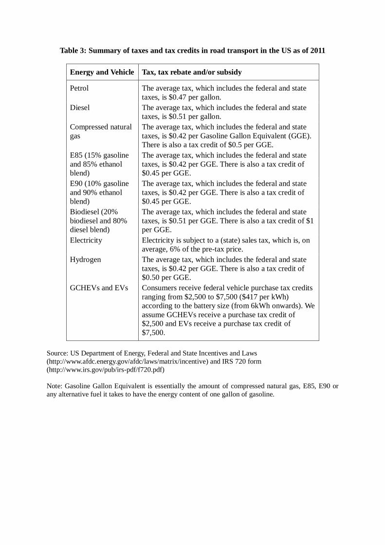
Table 3: Summary of taxes and tax credits in road transport in the US as of 2011

Energy and Vehicle Tax, tax rebate and/or subsidy

Petrol The average tax, which includes the federal and state

taxes, is $0.47 per gallon.

Diesel The average tax, which includes the federal and state

taxes, is $0.51 per gallon.

Compressed natural

gas

The average tax, which includes the federal and state

taxes, is $0.42 per Gasoline Gallon Equivalent (GGE).

There is also a tax credit of $0.5 per GGE.

E85 (15% gasoline

and 85% ethanol

blend)


taxes, is $0.42 per GGE. There is also a tax credit of

$0.45 per GGE.

E90 (10% gasoline

and 90% ethanol

blend)



$0.45 per GGE.

Biodiesel (20%

biodiesel and 80%

diesel blend)


taxes, is $0.51 per GGE. There is also a tax credit of $1

per GGE.

Electricity Electricity is subject to a (state) sales tax, which is, on

average, 6% of the pre-tax price.

Hydrogen The average tax, which includes the federal and state


$0.50 per GGE.

GCHEVs and EVs Consumers receive federal vehicle purchase tax credits

ranging from $2,500 to $7,500 ($417 per kWh)

according to the battery size (from 6kWh onwards). We

assume GCHEVs receive a purchase tax credit of

$2,500 and EVs receive a purchase tax credit of

$7,500.

Source: US Department of Energy, Federal and State Incentives and Laws

(http://www.afdc.energy.gov/afdc/laws/matrix/incentive) and IRS 720 form

(http://www.irs.gov/pub/irs-pdf/f720.pdf)

Note: Gasoline Gallon Equivalent is essentially the amount of compressed natural gas, E85, E90 or

any alternative fuel it takes to have the energy content of one gallon of gasoline.

https://nexus.ox.ac.uk/owa/redir.aspx?C=76a861bf3f894e76a7f1fe53f428b7ae&URL=http%3a%2f%2fwww.afdc.energy.gov%2fafdc%2flaws%2fmatrix%2fincentive

Table 4: Possible policies under a 6% and 60% discount rates

No tax change

Gasoline and diesel tax increases to $1

PVC breaks even in

PVC breaks even in

10 years 6 years 2 years 10 years 6 years 2 years

60% GIHEV 2,569 2,609 2,853 2,425 2,472 2,763

GCHEV 5,945 6,006 6,381 5,724 5,796 6,242

EV 12,719 12,803 13,289 12,274 12,380 13,009

CICEBD 1,884 1,894.5 1,970 1,439 1471 1,691

SDEICEV 343 358 449 -102 -65 169

6% GIHEV 435 1,296 2,515 -96.5 909 2,356

GCHEV 2,672 3,993 5,863 1,856 3,398.5 5,618

EV 8,355 10,195.5 12,650 6,712 4,9760 12,157

CICEBD 1,258 1,482 1,858 -385 285 1,365

SDEICEV -362.5 -30 432.5 -2,005.5 -1,227 -60

Note: Positive numbers are subsidies. Negative numbers are taxes. All current taxes and tax credits,

summarised in Table 4, stay the same except for the vehicle subsidies proposed here and the gasoline

and diesel taxes, which are increased to 1$/gallon. We do not include external costs in the calculations

for two reasons: first, consumers do not include them and most importantly, we have already showed

that these are negligible in any case.

Figure 1: Well-to-Pump CO2e emissions in the US for 2020

Source: estimates produced by GREET 1.8b

-50

0

50

100

150

200

SIC

EG

SID

IG

CIC

ED

SIC

EC

NG

SF

FIC

EV

SD

EIC

EV

CIC

EB

D

GIH

EV

GC

HE

V

EV

FC

VH

FC

VM

WT

P

CO

2 e

(g/k

m)

Vehicle/Fuel Systems

Fossil Fuel Vehicles Biofuel Vehicles Hybrid Electric Vehicles Electric Vehicles Fuel Cell Vehicles

Figure 2: Pump-to-Wheel CO2e emissions in the US for 2020


0

50

100

150

200

250

SIC

EG

SID

IG

CIC

ED

SIC

EC

NG

SF

FIC

EV

SD

EIC

EV

CIC

EB

D

GIH

EV

GC

HE

V

EV

FC

VH

FC

VM

PT

W C

O2 e

(g/k

m)

Vehicle/Fuel Systems

Fossil Fuel Vehicles Biofuel Vehicles Hybrid Electric Vheicles Electric Vehicles Fuel Cell Vehicles

Figure 3 Well-to-Wheel CO2e emissions in the US for 2020


Figure 4: Vehicle lifecycle CO2e emissions in the US for 2020

Source: Values taken from GREET 2 database

Source: see text

Figure 5: Integrated CO2e emissions from different vehicle/fuel systems in the US for 2020 (including both vehicle and fuel lifecycles)

Source: Figures 3 and 4 of the present paper

0

10

20

30

40

50

60

70

80

90

100

0 50000 100000 150000 200000 250000 300000

CO

2 e

ton

nes

/veh

icle

Distance Vehicle Traveled (km)

SICEG

SIDIG

CICED

SICECNG

SFFICEV

SDEICEV

CICEBD

GIHEV

GCHEV

EV

FCVH

FCVM

Figure 6: Breakeven points including private and environmental costs (excluding all taxes and subsidies)

Source: see text

Figure 7: Breakeven points including private costs only (excluding all taxes and subsidies)

Source: see text

22,000

24,000

26,000

28,000

30,000

32,000

34,000

36,000

38,000

40,000

2010 2011 2012 2013 2014 2015 2016 2017 2018 2019 2020

Pri

va

te C

os

ts (

$)

Year

SICEG

CICED

SICECNG

SFFICEV

SDEICEV

CICEBD

GIHEV

GCHEV

EV

SIDIG

Figure 8: Breakeven points including private costs only (and including taxes and subsidies from Table 3)

Source: see text

22,000

24,000

26,000

28,000

30,000

32,000

34,000

36,000

38,000

40,000

2010 2011 2012 2013 2014 2015 2016 2017 2018 2019 2020

Pri

va

te C

osts

($

)

Year

SICEG

CICED

SICECNG

SFFICEV

SDEICEV

CICEBD

GIHEV

GCHEV

EV

SIDIG

decarbonising the road transport sector: breakeven point

Documents