d.ebert_procedural modeling, animation, and rendering of gases, fluids, and textures

8/7/2019 D.Ebert_Procedural Modeling, Animation, and Rendering of Gases, Fluids, and Textures

http://slidepdf.com/reader/full/debertprocedural-modeling-animation-and-rendering-of-gases-fluids-and 1/35

Chapter 3:

Procedural Modeling, Animation, and Rendering of Gases, Fluids,and Textures

David S. Ebert

3.1 Introduction

This chapter describes modeling and animating procedural t extures, gases, and liquids. The main thrust

of the chapter is on procedurally modeling and animating volume density functions for creating realistic

images and animations of gases and fluids. A volume density function is a three-dimensional function(v f d ( x ; y ; z ) ) that defines the density of a continuous three-dimensional space. By using volume rendering

techniques[5], volume density functions can create volumetric gases and fluids. Volume density functions

are the natural extension of solid texturing to describing the actual geometry of the object.

Volume density functions are being used extensively in computer graphics for modeling and animating

gases, fire, fur, liquids, and other ‘‘soft’’ objects. I have used them extensively for modeling and animating

gases such as steam and fog [2, 7, 5, 3]. Hypertextures [18], metaballs [22](also called implicit surfaces and

soft objects), and Inakage’s flames [10] are other examples of the use of volume density functions.

As mentioned above, this chapter described how to model and animate volumetric gases. Therefore, I

should first explain why we want to model and animate gases in computer graphics. There are two reasons.

First, we need gases for visual realism. Gases such as fog, steam, smoke, and clouds are a part of oureveryday environment. In order to create realistic images of our environment, these gases must be included.

Both indoor and outdoor scenes benefit from the addition of gases. The realism and mood of outdoor scenes,

such as a dark, dreary forest can be increased greatly by the addition of elements such as fog. Realism of

indoor scenes can also be enhanced by the inclusion of steam rising from a cup of coffee or smoke from

a fireplace. Second, gases can be used for artistic effects. As the movie director uses fog machines and

similar devices to set the stage of his drama, so can the computer animator use computer generated fog (and

other gases) for dramatic effects.

There have been several previous approaches to modeling gases in computer graphics. Kajiya, [11], has

used a simple physical approximation for the formation and animation of clouds. Gardner, [8], has use solid

textured hollow ellipsoids in modeling clouds and more recently produced animations of smoke rising from

a forest fire [9]. Other approaches include the use of height fields [14], constant density media [13, 15], and

fractals [21]. The author has developed several approaches for modeling and controlling the animation of

3-1



gases [2, 7, 5, 3, 1]. Recently, Stam has used ‘‘fuzzy blobbies’’ as a three-dimensional model for animating

gases with good results [20].

The purpose of these notes is to describe my design approach for modeling, rendering, and animating

gases. These notes will help explain how my approach developed and also show the development of several

example procedures.

In the discussion that follows, an overview of gas rendering issues is discussed. Next, a brief description

of the development of my approach to modeling and animating gases, called solid spaces is presented,

followed by an in-depth description of the modeling of the gases and fluids. Finally, animation techniques

for solid textures, hypertextures, and gases are thoroughly discussed, including detailed descriptions of

several example procedures.

3.1.1 Overview of the Rendering System

For realistic images and animations of gases, volume rendering must be performed. While any procedure-

based volume rendering system can be used such as the the system described by Perlin in [18], we will

look at my system which is described in detail in [5] and [7]. This hybrid rendering system uses a fast

scanline a-buffer rendering algorithm for the surface-defined objects in the scene, while volume modeled

objects are volume rendered. The algorithm first creates the a-buffer for a scanline containing a list for

each pixel of all the fragments that partially or fully cover the pixel. Then for each volume that covers

this scanline, the volume rendering is performed next, creating a-buffer fragments for the separate sections

of the volumes. Volume rendering ceases once full coverage of the pixel by volume or surfaced-defined

elements is achieved. Finally, these volume a-buffer fragments are sorted into the a-buffer fragment list

based on their average Z-depth values and the a-buffer fragment list is rendered to produce the final color

of the pixel. The rendering system features a physically-based low-albedo illumination and atmospheric

attenuation model for the gases. Volumetric shadows are also efficiently combined into the system through

the use of three-dimensional shadow tables[4].

3.2 Solid Spaces

3.2.1 Development of Solid Spaces

The approach I have taken to modeling and animating gases started with work in solid texturing. Solid

texturing can be viewed as creating a three-dimensional color space that surrounds the object. When you

apply the solid texture to the object, you are simply carving away the defining space. I was experimenting

with creating a wide range of solid texture functions, most of which were based on Perlin’s turbulence

and noise functions [16] when he was asked to produce an image of a butterfly emerging from mist or

fog. The idea of solid texturing multiple object characteristics was already part of my rendering system. I

decided to use solid textured transparency to produce layers of fog/clouds. The solid texturing function was

based on turbulence, since these phenomena are created through turbulent flow. This approach is similar to

3-2



Gardner’s approach [8]. The next extension was to use turbulence-based procedures to define the density of

three-dimensional volumes instead of controlling the transparency of hollow surfaces. As you can see, the

idea of using three-dimensional spaces to represent object attributes such as color, transparency, and even

geometry is emerging as a common theme in this progression. The system for representing object attributes

using this idea is termed solid spaces. The solid space framework encompasses traditional solid texturing,

hypertextures, and other techniques within a unified framework.

3.2.2 What are Solid Spaces

Solid spaces are three-dimensional spaces associated with an object that allow for control of an attribute of

the object. For instance, in solid texturing the texture space is a solid space associated with the object that

defines the color of each point in the volume that the object occupies. This space can be considered to be

associated with, or represent, the space of the material from which the object is created (material space).

Solid spaces have many uses in describing object attributes. For a more detailed description of the uses of

solid spaces, please see [2, 4, 5, 7].

3.3 Geometry of the Gases

As mentioned in the introduction, the geometry of the gases is modeled using turbulent flow based volume

density functions. I have used a ‘‘visual simulation’’ of turbulent flow similar to Ken Perlin’s approach [16].

The volume density functions take the location of the point in world space, find it’s corresponding location

in the turbulence space (a three-dimensional space), and apply the turbulence function. The value returned

by the turbulence function is used as the basis for the gas density and is then ‘‘shaped’’ to simulate the type

of gas desired by using simple mathematical functions. (My implementation of noise and turbulence can be

found in [4].) In the discussion that follows, the use of basic mathematical functions for shaping the gas is

described followed by the development of several example procedures for modeling the geometry of the

gases.

3.3.1 Basic Gas Shaping

Several basic mathematical functions are used to shape the geometry of the gas. The first of these is the

power function. Let’s look at a simple procedure for modeling a gas and see the effects of the power

function, and other functions on the resulting shape of the gas.

3-3



basic_gas(pnt,density,parms)

xyz_td pnt;

float *density,*parms;

{

float turb;

int i;

static float pow_table[POW_TABLE_SIZE];static int calcd=1;

if(calcd)

{ calcd=0;

for(i=POW_TABLE_SIZE-1; i>=0; i--)

pow_table[i] = (float)pow(((double)(i))/(POW_TABLE_SIZE-1)*

parms[1]*2.0,(double)parms[2]);

}

turb =fast_turbulence(pnt);

*density = pow_table[(int)(turb*(.5*(POW_TABLE_SIZE-1)))];

}

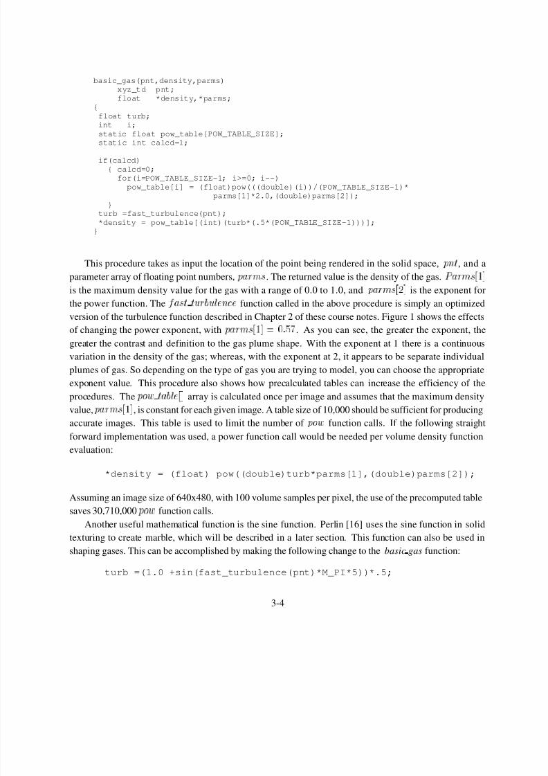
This procedure takes as input the location of the point being rendered in the solid space, p n t , and a

parameter array of floating point numbers, p a r m s . The returned value is the density of the gas. P a r m s 1

is the maximum density value for the gas with a range of 0.0 to 1.0, and p a r m s 2 is the exponent for

the power function. The f a s t t u r b u l e n c e function called in the above procedure is simply an optimized

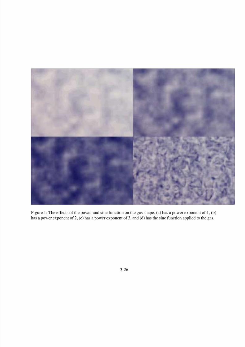
version of the turbulence function described in Chapter 2 of these course notes. Figure 1 shows the effects

of changing the power exponent, with p a r m s 1 ] = 0 5 7 . As you can see, the greater the exponent, the

greater the contrast and definition to the gas plume shape. With the exponent at 1 there is a continuous

variation in the density of the gas; whereas, with the exponent at 2, it appears to be separate individual

plumes of gas. So depending on the type of gas you are trying to model, you can choose the appropriate

exponent value. This procedure also shows how precalculated tables can increase the efficiency of the

procedures. The p o w t a b l e array is calculated once per image and assumes that the maximum density

value, p a r m s 1 , is constant for each given image. A table size of 10,000 should be sufficient for producing

accurate images. This table is used to limit the number of p o w function calls. If the following straight

forward implementation was used, a power function call would be needed per volume density function

evaluation:

*density = (float) pow((double)turb*parms[1],(double)parms[2]);

Assuming an image size of 640x480, with 100 volume samples per pixel, the use of the precomputed table

saves 30,710,000 p o w function calls.

Another useful mathematical function is the sine function. Perlin [16] uses the sine function in solid

texturing to create marble, which will be described in a later section. This function can also be used in

shaping gases. This can be accomplished by making the following change to the basic gas function:

turb =(1.0 +sin(fast_turbulence(pnt)*M_PI*5))*.5;

3-4



The sine function has a similar effect as in its use for marble: the above change creates ‘‘veins’’ in the

shape of the gas. As you can see from these simple examples, it is very easy to shape the gas using simple

mathematical functions. Next, we’ll see how to produce more complex shapes in the gas.

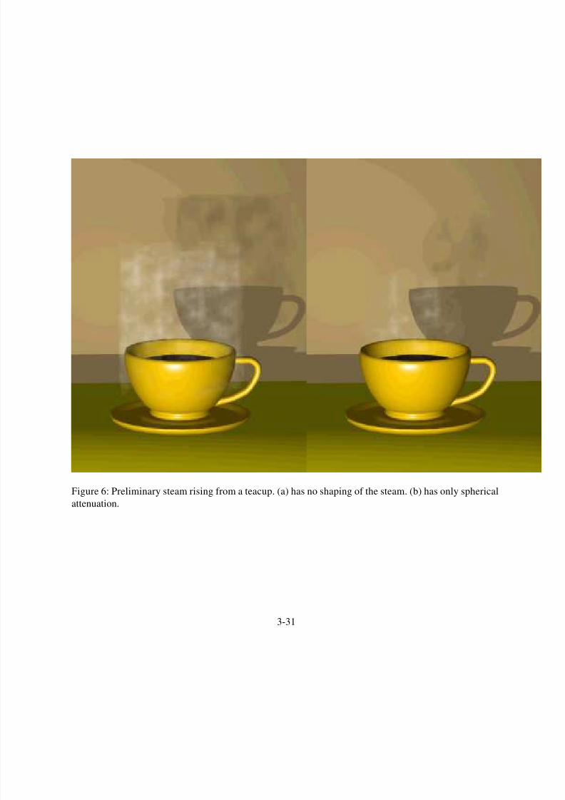
3.3.2 Steam Rising From a Teacup

The goal is the to create a realistic image of steam rising from a teacup. The first step is to place a

‘‘slab’’ [12] of volume gas over the teacup. (Any raytracable solid can be used for defining the extent of

the volume.) Since steam is not a very thick gas, a maximum density value of 0.57 will be used with an

exponent of 6.0 for the power function. The resulting image can be seen in Figure 6(a). This was produced

from the above b a s i c g a s procedure.

The image created, however, does not look like steam rising from a teacup. First of all, the steam is

not confined to be only above and over the cup. Secondly, the steam’s density does not decrease as it rises.

These problems can be easily corrected. First, ramp off the density spherically from the center of the top

of the coffee. This will make the steam be only within the radius of the cup and will make the steam rise

higher over the center of the cup. The following addition to the basic gas procedure will accomplish this:

steam_slab1(pnt, pnt_world, density,parms, vol)xyz_td pnt, pnt_world;float *density,*parms;vol_td vol;

{float turb;int i;xyz_td distance;static float pow_table[POW_TABLE_SIZE], ramp[RAMP_SIZE];static int calcd=1;

if(calcd){ calcd=0;

for(i=POW_TABLE_SIZE-1; i>=0; i--)pow_table[i] = (float)pow(((double)(i))/(POW_TABLE_SIZE-1)*

parms[1]*2.0,(double)parms[2]);make_ramp_table(ramp);}

turb =fast_turbulence(pnt);*density = pow_table[(int)(turb*0.5*(POW_TABLE_SIZE-1))];

/* determine distance from center of the slab ^2. */XYZ_SUB(diff,vol.shape.center, pnt_world);dist_sq = DOT_XYZ(diff,diff);density_max = dist_sq*vol.shape.inv_rad_sq.y;indx = (int)((pnt.x+pnt.y+pnt.z)*100) & (OFFSET_SIZE -1);density_max += parms[3]*offset[indx];

if(density_max >= .25) /* ramp off if > 25% from center */{ i = (density_max -.25)*4/3*RAMP_SIZE; /* get table index 0:RAMP_SIZE-1 */

i=MIN(i,RAMP_SIZE-1);density_max = ramp[i];

*density *=density_max;}}

make_ramp_table(ramp)

3-5



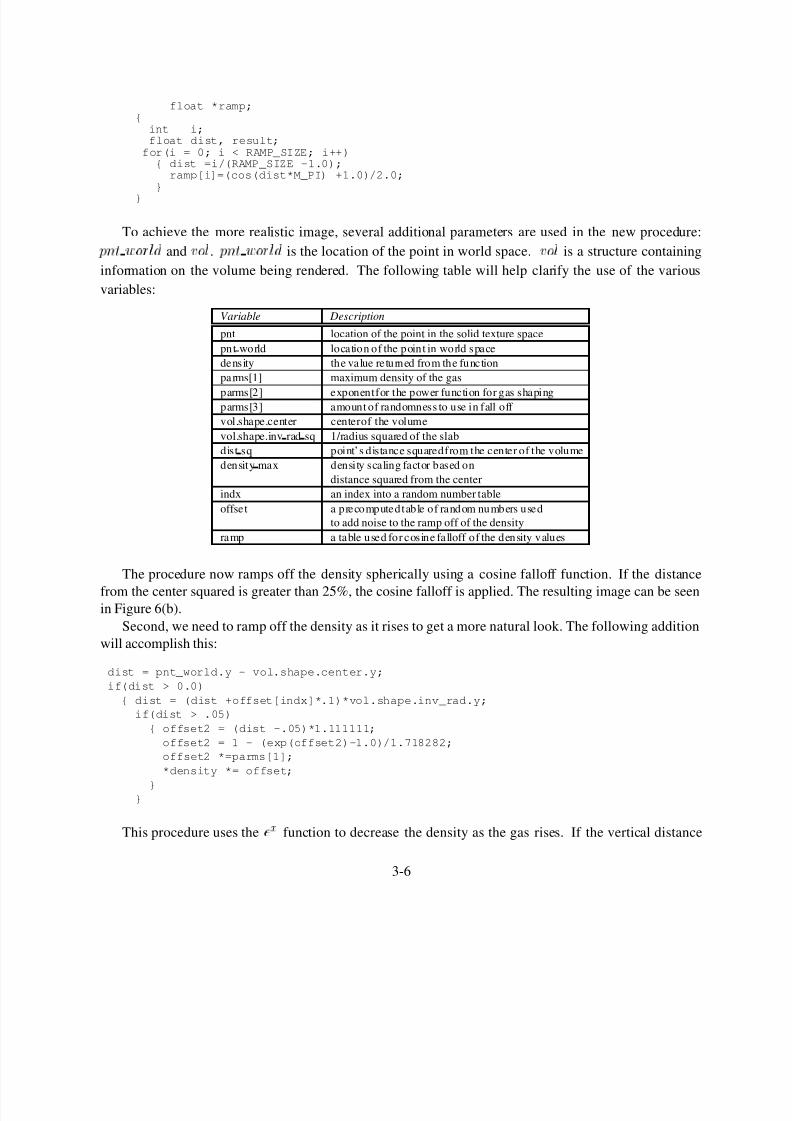
float *ramp;{

int i;float dist, result;

for(i = 0; i < RAMP_SIZE; i++){ dist =i/(RAMP_SIZE -1.0);

ramp[i]=(cos(dist*M_PI) +1.0)/2.0;}

}

To achieve the more realistic image, several additional parameters are used in the new procedure:

p n t w o r l d and v o l . p n t w o r l d is the location of the point in world space. v o l is a structure containing

information on the volume being rendered. The following table will help clarify the use of the various

variables:

Variable Description

pnt location of the point in the solid texture space

pnt world location of the point in world s pace

dens ity the value returned from the function

pa rms[1] maximum density of the gas

parms[2] exponentfor the power function for gas shapingparms[3] amount of randomness to use in fall off

vol.shape.center centerof the volume

vol.shape.inv rad sq 1/radius squared of the slab

dist sq point’s distance squaredfrom the center of the volume

density max density scaling factor based on

distance squared from the center

indx an index into a random number table

offset a precomputedtable of random numbers used

to add noise to the ramp off of the density

ramp a table used for cos ine falloff of the density values

The procedure now ramps off the density spherically using a cosine falloff function. If the distance

from the center squared is greater than 25%, the cosine falloff is applied. The resulting image can be seenin Figure 6(b).

Second, we need to ramp off the density as it rises to get a more natural look. The following addition

will accomplish this:

dist = pnt_world.y - vol.shape.center.y;

if(dist > 0.0)

{ dist = (dist +offset[indx]*.1)*vol.shape.inv_rad.y;

if(dist > .05)

{ offset2 = (dist -.05)*1.111111;

offset2 = 1 - (exp(offset2)-1.0)/1.718282;

offset2 *=parms[1];

*density *= offset;

}}

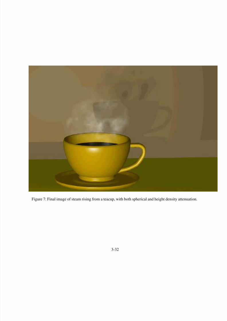
This procedure uses thee

x function to decrease the density as the gas rises. If the vertical distance

3-6



above the center is greater than 5% of the total distance, the density is exponentially ramped off to 0. The

results of this addition to the above procedure can be seen in Figure 7. As you can see in this image, the

resulting steam is very convincing. In a later section animation effects using this basic steam model will be

presented.

3.3.3 A Single Column of Smoke

The final example procedure that I will describe creates a single column of rising smoke. For this smoke

column, the basis is a vertical cylinder. By deforming this shape, we can create a realistic smoke column.

The obvious visual characteristics of a smoke column are that is it disperses as it rises and that it is initially

smooth and becomes more turbulent as it rises. Turbulence can be added to the cylinder’s center to make a

more natural looking smoke column. To simulate turbulent effect and air currents, the amount of turbulence

is increased as a function of the height of the smoke column. Also, you need to decrease the density as

a function of height to help simulate the dispersion. These ideas, which are similar to the steam rising

procedure, are only the start to a realistic column of smoke. The shape also needs to be bent and swirled as

the smoke rises. This can be achieved by using a vertical helix to displace each point before calculating its

distance from the center of the cylinder. A more detailed description of this procedure can be found in [4].

3.4 Animating Solid Spaces

Now that you have seen how to model the geometry of the gases, a discussion of animating these gas

procedures and other solid space procedures will be presented. There are several ways that solid spaces can

be animated. These notes will consider two approaches:

Changing the solid space over time.

Moving the point being rendered through the solid space.

The first approach has time as a parameter which changes the definition of the space over time. This is

a very natural and obvious way to animate procedural techniques.

The second approach is to not change the solid space, but actually move the point in the volume or

object over time through the space. The movement of the gas (solid texture, hypertexture) is created by

moving the fixed three-dimensional screen space point along a path over time through the turbulence space

before evaluating the turbulence function. Each three-dimensional screen space point is inversely mapped

back to world space. Then from world space, it is mapped into the gas and turbulence space through the use

of simple affine transformations. Finally, it is moved through the turbulence space over time to create the

movement. Therefore, the path direction will have the reverse visual effect. For example, a downward path

applied to the screen space point will show the texture or volume object rising.

Both of these techniques can be applied to solid texturing, gases, and hypertextures. The application of

these techniques to solid texturing will be discussed first, followed by the use of these techniques for gas

animation, and finally, the use of these techniques for hypertextures, including liquids and fire.

3-7



3.5 Animating Solid Textures

The previous section described two animation approaches. This section will show how these approaches

can be used for solid texturing. The use of these two approaches for color solid texturing will be presented

first, followed by a discussion of these approaches for solid textured transparency.

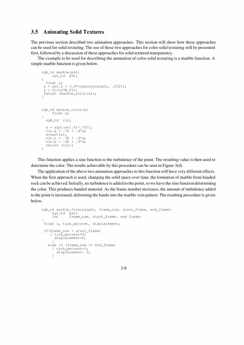
The example to be used for describing the animation of color solid texturing is a marble function. Asimple marble function is given below.

rgb_td marble(pnt)xyz_td pnt;

{float y;

y = pnt.y + 3.0*turbulence(pnt, .0125);y = sin(y*M_PI);return (marble_color(x));

}

rgb_td marble_color(x)float x;

{

rgb_td clr;

x = sqrt(x+1.0)*.7071;clr.g = .30 + .8*x;x=sqrt(x);clr.r = .30 + .6*x;clr.b = .60 + .4*x;return (clr);

}

This function applies a sine function to the turbulence of the point. The resulting value is then used to

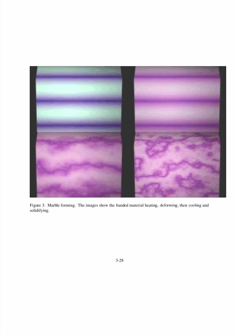
determine the color. The results achievable by this procedure can be seen in Figure 3(d).

The application of the above two animation approaches to this function will have very different effects.

When the first approach is used, changing the solid space over time, the formation of marble from banded

rock can be achieved. Initially, no turbulence is added to the point, so we have the sine function determining

the color. This produces banded material. As the frame number increases, the amount of turbulence added

to the point is increased, deforming the bands into the marble vein pattern. The resulting procedure is given

below.

rgb_td marble_forming(pnt, frame_num, start_frame, end_frame)xyz_td pnt;int frame_num, start_frame, end_frame;

{float x, turb_percent, displacement;

if(frame_num < start_frame){ turb_percent=0;

displacement=0;

}else if (frame_num >= end_frame)

{ turb_percent=1;displacement= 3;

}

3-8



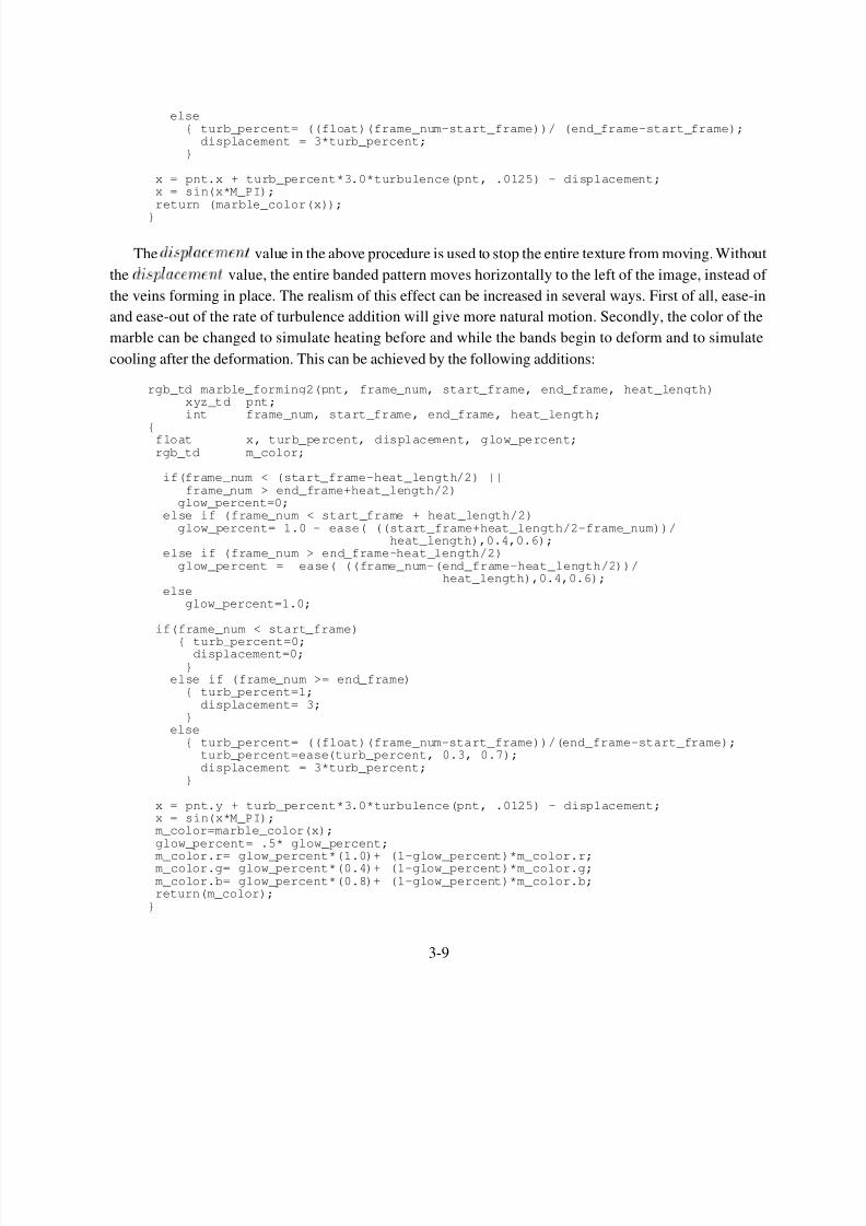
else{ turb_percent= ((float)(frame_num-start_frame))/ (end_frame-start_frame);

displacement = 3*turb_percent;}

x = pnt.x + turb_percent*3.0*turbulence(pnt, .0125) - displacement;x = sin(x*M_PI);return (marble_color(x));

}

The d i s p l a c e m e n t value in the above procedure is used to stop the entire texture from moving. Without

the d i s p l a c e m e n t value, the entire banded pattern moves horizontally to the left of the image, instead of

the veins forming in place. The realism of this effect can be increased in several ways. First of all, ease-in

and ease-out of the rate of turbulence addition will give more natural motion. Secondly, the color of the

marble can be changed to simulate heating before and while the bands begin to deform and to simulate

cooling after the deformation. This can be achieved by the following additions:

rgb_td marble_forming2(pnt, frame_num, start_frame, end_frame, heat_length)xyz_td pnt;int frame_num, start_frame, end_frame, heat_length;

{float x, turb_percent, displacement, glow_percent;rgb_td m_color;

if(frame_num < (start_frame-heat_length/2) ||frame_num > end_frame+heat_length/2)

glow_percent=0;else if (frame_num < start_frame + heat_length/2)

glow_percent= 1.0 - ease( ((start_frame+heat_length/2-frame_num))/heat_length),0.4,0.6);

else if (frame_num > end_frame-heat_length/2)glow_percent = ease( ((frame_num-(end_frame-heat_length/2))/

heat_length),0.4,0.6);else

glow_percent=1.0;

if(frame_num < start_frame)

{ turb_percent=0;displacement=0;}

else if (frame_num >= end_frame){ turb_percent=1;

displacement= 3;}

else{ turb_percent= ((float)(frame_num-start_frame))/(end_frame-start_frame);

turb_percent=ease(turb_percent, 0.3, 0.7);displacement = 3*turb_percent;

}

x = pnt.y + turb_percent*3.0*turbulence(pnt, .0125) - displacement;x = sin(x*M_PI);m_color=marble_color(x);glow_percent= .5* glow_percent;

m_color.r= glow_percent*(1.0)+ (1-glow_percent)*m_color.r;m_color.g= glow_percent*(0.4)+ (1-glow_percent)*m_color.g;m_color.b= glow_percent*(0.8)+ (1-glow_percent)*m_color.b;return(m_color);

}

3-9



The resulting images can be seen in Figure 3. Of course the resulting sequence would be even more

realistic if the material actually deformed, instead of the color simplychanging. This effect will be described

in a later section.

A different effect can be achieved by the second animation approach, moving the point through the

solid space. The procedure below moves the point along a helical path before evaluating the turbulence

function. This produces the effect of the marble pattern moving through the object. This technique can be

used by a designer in determining the portion of marble to ‘‘cut’’ his/her object from in order to achieve the

most pleasing vein patterns.

rgb_td moving_marble(pnt, frame_num)xyz_td pnt;int frame_num;

{float x, tmp, tmp2;static float down, theta, sin_theta, cos_theta;xyz_td hel_path, direction;static int calcd=1;

if(calcd){ theta =(frame_num%SWIRL_FRAMES)*SWIRL_AMOUNT; /* swirling effect */

cos_theta = RAD1 * cos(theta) + 0.5;sin_theta = RAD2 * sin(theta) - 2.0;down = (float)frame_num*DOWN_AMOUNT+2.0;calcd=0;

}tmp = fast_noise(pnt); /* add some randomness */tmp2 = tmp*1.75;

/* calculate the helical path */hel_path.y = cos_theta2 + tmp;hel_path.x = (- down) + tmp2;hel_path.z = sin_theta2 - tmp2;XYZ_ADD(direction, pnt, hel_path);

x = pnt.y + 3.0*turbulence(direction, .0125);x = sin(x*M_PI);return (marble_color(x));

}

In the above procedure, S W I R L F R A M E S = 1 2 6 and S W I R L A M O U N T = 2 = 1 2 6 . This

produces the path swirling every 126 frames. D O W N A M O U N T = 0 0 0 9 5 and controls the speed of

the downward movement along the helical path. R A D 1 and R A D 2 are the y and z radii of the helical path.

3.5.1 Animating Solid Textured Transparency

The previous section described two different ways that solid space functions can be animated for color

solid texturing and the results achievable by both techniques. This section describes the use of animation

techniques for solid textured transparency.

The animation technique of moving the point through the solid space was my original animationtechnique. The results of this technique applied to solid textured transparency can be seen in [1]. The

following procedure, which is similar in animation techniques to the above m o v i n g m a r b l e procedure,

3-10



produces fog moving through the surface of an object. Again, a downward helical path is used for the

movement through the space. This produces an upward swirling to the gas movement.

void fog(pnt,*transp, frame_num)xyz_td pnt;float *transp;int frame_num

{float tmp;xyz_td direction,cyl;double theta;

pnt.x += 2.0 +turbulence(pnt, .1);tmp = noise_it(pnt);pnt.y += 4+tmp;pnt.z += -2 - tmp;

theta =(frame_num%SWIRL_FRAMES)*SWIRL_AMOUNT;cyl.x =RAD1 * cos(theta);cyl.z =RAD2 * sin(theta);

direction.x = pnt.x + cyl.x;direction.y = pnt.y - frame_num*DOWN_AMOUNT;direction.z = pnt.z + cyl.z;

*transp = turbulence(direction, .015);*transp = (1.0 -(*transp)*(*transp)*.275);*transp =(*transp)*(*transp)*(*transp);

}

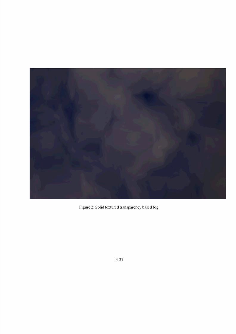
A still of this procedure applied to a cube can be seen in Figure 2. For these images, the following values

were used: D O W N A M O U N T = 0 0 0 9 5 , S W I R L F R A M E S = 1 2 6 , and S W I R L A M O U N T =

2 = 1 2 6 , R A D 1 = 0 1 2 , and R A D 2 = 0 0 8 .This technique is similar to Gardner’s technique for

producing images of clouds [8], except that it uses turbulence to control the transparency instead of Fourier

synthesis.

3.6 Animation of Gaseous Volumes

As described in a previous section, the movement of the gas is created by movingthe fixed three-dimensional

screen space point along a path over time through the turbulence space before evaluating the turbulence

function. Each three-dimensional screen space point is inversely mapped back to world space. Then from

world space, it is mapped into the gas and turbulence space through the use of simple affine transformations.

Finally, it is moved through the turbulence space over time to create the movement of the gas. Therefore,

the path direction will have the reverse visual effect. For example, a downward path applied to the screen

space point will show the gas as rising.

Several interesting animation effects can be achieved through the use of simple helical paths for the

movement through the solid space. A discussion of these effects is presented first, followed by a discussion

of the use of three-dimensional tables for controlling the gas movement. Finally, several additional primitive

functions for creating gas animation will be presented. The second animation technique, moving the point

through the gas space, is used in all the procedures in this section.

3-11



Helical Path Effects

As mentioned above, helical paths can be used to create several different animation effects for gases.

Earlier in these notes, a procedure for producing a still image of steam rising from a teacup was described.

This procedure can be modified to produce convincing animations of steam rising from the teacup by the

addition of helical paths for motion. The modification needed is given below. This is the same technique

that was used in the moving marble function.

steam_moving(pnt, pnt_world, density,parms, vol)xyz_td pnt, pnt_world;float *density,*parms;vol_td vol;

{float tmp,turb, dist_sq, density_max, offset2, theta, dist;static float ramp[RAMP_SIZE];extern float offset[OFFSET_SIZE];extern int frame_num;xyz_td direction, diff;int i, indx;static float pow_table[POW_TABLE_SIZE];static int calcd=1;

static float down, cos_theta2, sin_theta2;

if(calcd){ calcd=0;

/* determine how to move the point through the space (helical path) */theta =(frame_num%SWIRL_FRAMES)*SWIRL;down = (float)frame_num*DOWN*3.0 +4.0;cos_theta2 = RAD1*cos(theta) +2.0;sin_theta2 = RAD2*sin(theta) -2.0;

for(i=POW_TABLE_SIZE-1; i>=0; i--)pow_table[i] = (float)pow(((double)(i))/(POW_TABLE_SIZE-1)*

parms[1]*2.0,(double)parms[2]);make_ramp_table(ramp);

}

tmp = fast_noise(pnt);

direction.x = pnt.x + cos_theta2 +tmp;direction.y = pnt.y - down + tmp;direction.z = pnt.z +sin_theta2 +tmp;

turb =fast_turbulence(direction);*density = pow_table[(int)(turb*0.5*(POW_TABLE_SIZE-1))];

/* determine distance from center of the slab ^2. */XYZ_SUB(diff,vol.shape.center, pnt_world);dist_sq = DOT_XYZ(diff,diff);density_max = dist_sq*vol.shape.inv_rad_sq.y;indx = (int)((pnt.x+pnt.y+pnt.z)*100) & (OFFSET_SIZE -1);density_max += parms[3]*offset[indx];

if(density_max >= .25) /* ramp off if > 25% from center */{ i = (density_max -.25)*4/3*RAMP_SIZE; /* get table index 0:RAMP_SIZE-1 */

i=MIN(i,RAMP_SIZE-1);

density_max = ramp[i];*density *=density_max;}

/* ramp it off vertically */

3-12



dist = pnt_world.y - vol.shape.center.y;if(dist > 0.0)

{ dist = (dist +offset[indx]*.1)*vol.shape.inv_rad.y;if(dist > .05)

{ offset2 = (dist -.05)*1.111111;offset2 = 1 - (exp(offset2)-1.0)/1.718282;offset2*=parms[1];*density *= offset2;

}}

}

This function creates upward swirling movement in the gas, which swirls around 360 degrees every

SWIRL FRAMES frames. Noise is applied to the path so that it appears more random. The parameters

RAD1 and RAD2 determine the elliptical shape of the swirling path.

A downward helical path through the gas space produces the effect of the gas rising and swirling in the

opposite direction. The same technique can be used to produce animations of fog developing and rolling

by. A horizontal helical path creates the movement of the gas. A description of this can be found in [5].

For more realistic steam motion, a simulation of air currents is helpful. This can be approximated by

adding turbulence to the helical path. The amount of turbulence added will be proportional to the height

above the teacup with no turbulence added at the surface.

As shown above, a wide variety of effects can be achieved through the use of helical paths. This

requires the same type of path being used for movement throughout the entire volume of gas. Obviously,

more complex motion can be achieved by having different movement paths for different locations within

the gas. A three-dimensional table specifying different procedures for different locations within the volume

creates a flexible method for creating complex motion in this manner.

3.6.1 Three-dimensional tables

The use of three-dimensional tables (solid spaces) to control the animation of the gases is an extension tomy previous use of solid spaces in which three-dimensional tables were used for volume shadowing effects

[5].

The three-dimensional tables are handled in the following manner: the table surrounds the gas volume

in world space and values are stored at each of the lattice points in the table. These values represent the

calculated values for that specific location in the volume. To determine the values for other locations in the

volume, the eight table entries forming the parallelepiped surrounding the point are interpolated.

There are two types of tables for controlling the motion of the gases: vector field tables and functional

flow field tables. The vector field tables will not be described in detail in these notes. A thorough description

of their use and merits can be found in [7]. The vector field tables store direction vectors, density scaling

factors, and other information for their use at each point in the lattice. Thus, these tables are suited for

visualizing computational fluid dynamics simulations or using external programs for controlling the gas

movement[6].

3-13



The flow field function and vector field tables are incorporated into the volume density functions for

controlling the shape and movement of the gas. Each volume density function has a default path and

velocity for the gas movement. First, the default path and velocity are calculated, then the vector field tables

are evaluated and functions that calculate direction vectors, density scaling factors, etc., from the functional

flow field tables are applied. The default path vector, the vector from the vector field table, and the vector

from the flow field function are combined to produce the new path for the gas.

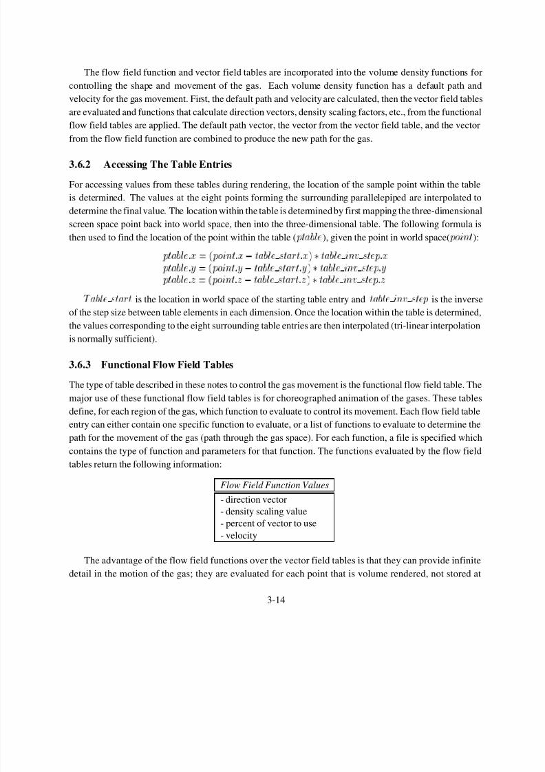
3.6.2 Accessing The Table Entries

For accessing values from these tables during rendering, the location of the sample point within the table

is determined. The values at the eight points forming the surrounding parallelepiped are interpolated to

determine the final value. The location within the table is determined by first mapping the three-dimensional

screen space point back into world space, then into the three-dimensional table. The following formula is

then used to find the location of the point within the table ( p t a b l e ), given the point in world space( p o i n t ):

p t a b l e : x = ( p o i n t : x ? t a b l e s t a r t : x ) t a b l e i n v s t e p : x

p t a b l e : y = ( p o i n t : y ? t a b l e s t a r t : y ) t a b l e i n v s t e p : y

p t a b l e : z = ( p o i n t : z ? t a b l e s t a r t : z ) t a b l e i n v s t e p : z

T a b l e s t a r t is the location in world space of the starting table entry and t a b l e i n v s t e p is the inverse

of the step size between table elements in each dimension. Once the location within the table is determined,

the values corresponding to the eight surrounding table entries are then interpolated (tri-linear interpolation

is normally sufficient).

3.6.3 Functional Flow Field Tables

The type of table described in these notes to control the gas movement is the functional flow field table. The

major use of these functional flow field tables is for choreographed animation of the gases. These tables

define, for each region of the gas, which function to evaluate to control its movement. Each flow field table

entry can either contain one specific function to evaluate, or a list of functions to evaluate to determine the

path for the movement of the gas (path through the gas space). For each function, a file is specified which

contains the type of function and parameters for that function. The functions evaluated by the flow field

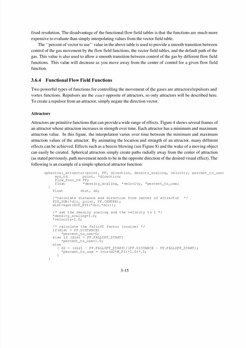
tables return the following information:

Flow Field Function Values

- direction vector

- density scaling value

- percent of vector to use

- velocity

The advantage of the flow field functions over the vector field tables is that they can provide infinite

detail in the motion of the gas; they are evaluated for each point that is volume rendered, not stored at

3-14



fixed resolution. The disadvantage of the functional flow field tables is that the functions are much more

expensive to evaluate than simply interpolating values from the vector field table.

The ‘‘percent of vector to use’’ value in the above table is used to provide a smooth transition between

control of the gas movement by the flow field functions, the vector field tables, and the default path of the

gas. This value is also used to allow a smooth transition between control of the gas by different flow field

functions. This value will decrease as you move away from the center of control for a given flow field

function.

3.6.4 Functional Flow Field Functions

Two powerful types of functions for controlling the movement of the gases are attractors/repulsors and

vortex functions. Repulsors are the exact opposite of attractors, so only attractors will be described here.

To create a repulsor from an attractor, simply negate the direction vector.

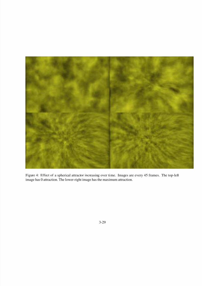
Attractors

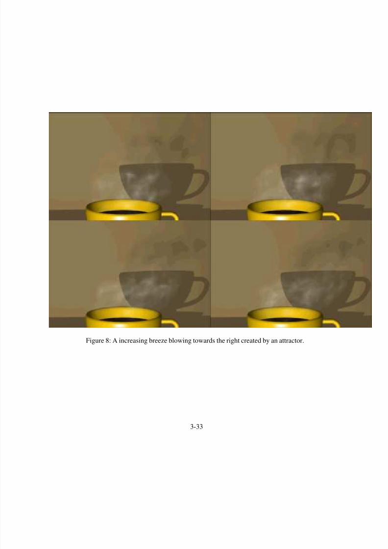
Attractors are primitive functions that can provide a wide range of effects. Figure 4 shows several frames of an attractor whose attraction increases in strength over time. Each attractor has a minimum and maximum

attraction value. In this figure, the interpolation varies over time between the minimum and maximum

attraction values of the attractor. By animating the location and strength of an attractor, many different

effects can be achieved. Effects such as a breeze blowing (see Figure 8) and the wake of a moving object

can easily be created. Spherical attractors simply create paths radially away from the center of attraction

(as stated previously, path movement needs to be in the opposite direction of the desired visual effect). The

following is an example of a simple spherical attractor function:

spherical_attractor(point, FF, direction, density_scaling, velocity, percent_to_use)xyz_td point, *directio n;flow_func_td FF;

float *density_scaling, *velocity, *percent_to_use;{

float dist, d2;

/*calculate distance and direction from center of attractor */XYZ_SUB(*dir, point, FF.CENTER);dist=sqrt(DOT_XYZ(*dir,*dir));

/* set the density scaling and the velocity to 1 */*density_scaling=1.0;*velocity=1.0;

/* calculate the falloff factor (cosine) */if(dist > FF.DISTANCE)

*percent_to_use=0;else if (dist < FF.FALLOFF_START)

*percent_to_use=1.0;

else{ d2 = (dist - FF.FALLOFF_START)/(FF.DISTANCE - FF.FALLOFF_START);

*percent_to_use = (cos(d2*M_PI)+1.0)*.5;}

}

3-15



The f l o w f u n c t d structure contains parameters for each instance of the spherical attractor. The param-

eters include the center of the attractor, FF.CENTER, the effective distance of attraction, FF.DISTANCE,

and where to begin the falloff from the attractor path to the default path, FF.FALLOFF START. This

function ramps the use of the attractor path from FF.FALLOFF START to FF.DISTANCE. A cosinefunction is used for a smooth transition between the path defined by the attractor and the default path of the

gas.

Extensions of Spherical Attractors

Variations on this simple spherical attractor include moving attractors, angle limited attractors, attractors

with variable maximum attraction, non-spherical attractors, and of course combinations of any or all of

these types. These variations can be animated over time to achieve more complex and interesting effects.

For example, the minimum and maximum attraction can be animated over time to produce the effects seen

in Figure 4 and Figure 8.

Instead of having the attraction be spherical in geometry, the geometry of the attraction can, for example,

be planar or linear. A linear attractor can be used for creating the flow of a gas along a wall, as will be

explained in a later section.

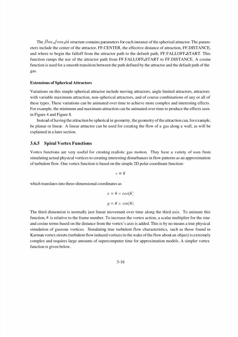
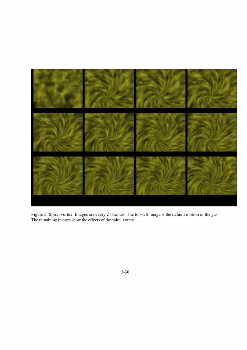
3.6.5 Spiral Vortex Functions

Vortex functions are very useful for creating realistic gas motion. They have a variety of uses from

simulating actual physical vortices to creating interesting disturbances in flow patterns as an approximation

of turbulent flow. One vortex function is based on the simple 2D polar coordinate function:

r =

which translates into three-dimensional coordinates as

x = c o s ( )

y = s i n ( )

The third dimension is normally just linear movement over time along the third axis. To animate this

function,

is relative to the frame number. To increase the vortex action, a scalar multiplier for the sine

and cosine terms based on the distance from the vortex’s axis is added. This is by no means a true physical

simulation of gaseous vortices. Simulating true turbulent flow characteristics, such as those found in

Karman vortex streets (turbulent flow induced vortices in the wake of the flow about an object) is extremelycomplex and requires large amounts of supercomputer time for approximation models. A simpler vortex

function is given below.

3-16



calc_vortex(pt, ff, path, velocity, percent_to_use, frame_num)

xyz_td *pt, *path;

flow_func_td *ff;

float *percent_to_use, *velocity;

int frame_num;

{

static tran_mat_td mat={0,0,0,0,0,0,0,0,0,0,0,0,0,0,0,0};xyz_td dir, pt2, diff;

float theta, dist, d2, dist2;

float cos_thet a,sin _t het a, compl _cos, ratio_mu lt;

/*calculate distance from center of vortex */

XYZ_SUB(diff,(*pt), ff->center);

dist=sqrt(DOT_XYZ(diff,diff));

dist2 = dist/ff->distance;

/* calculate angle of rotation about the axis */

theta = (ff->parms[0] *(1+.001*(frame_num)))/

(pow((.1+dist2*.9),ff->parms[1]));

/* calculate the matrix for rotating about the cylinder’s axis */

calc_rot_mat(theta, ff->axis, mat);

transform_XYZ((long)1,mat,pt,&pt2);XYZ_SUB(dir,pt2,(*pt));

path->x = dir.x;

path->y = dir.y;

path->z = dir.z;

/* Have the maximum strength increase from frame parms[4] to

* parms[5]to a maximum of parms[2] */

if(frame_num < ff->parms[4])

ratio_mult=0;

else if (frame_num <= ff->parms[5])

ratio_mult = (frame_num - ff->parms[4])/

(ff->parms[5] - ff->parms[4])* ff->parms[2];

else

ratio_mult = ff->parms[2];

/* calculate the falloff factor */if(dist > ff->distance)

{ *percent_to_use=0;

*velocity=1;

}

else if (dist < ff->falloff_start)

{ *percent_to_use=1.0 *ratio_mult;

/*calc velocity */

*velocity= 1.0+(1.0 - (dist/ff->falloff_start));

}

else

{ d2 = (dist - ff->falloff_start)/(ff->distance - ff->falloff_start);

percent_to_use = (cos(d2*M_PI)+1.0)*.5*ratio_mult;

*velocity= 1.0+(1.0 - (dist/ff->falloff_start));

}

}

This vortex function uses some techniques by Karl Sims [19]. For these vortices, the angle of rotation

about an axis is determined by both the frame number and the relative distance of the point from the center

3-17



*/

/* Have the maximum strength increase from frame parms[4] to* parms[5]to a maximum of parms[2]*/

if(frame_num < ff->parms[4])ratio_mult=0;

else if (frame_num <= ff->parms[5])

ratio_mult = (frame_num - ff->parms[4])/(ff->parms[5] - ff->parms[4])* ff->parms[2];

if(point.y < ff->parms[6])x_disp=0;

else{ if(point.y <= ff->parms[7])

d2 =COS_ERP((point.y - ff->parms[6])/(ff->parms[7] -ff->parms[6]));else

d2=0;x_disp = (1-d2)*ratio_mult*parms[8]+fast_noise(point)*ff->parms[9];

}return(x_disp);

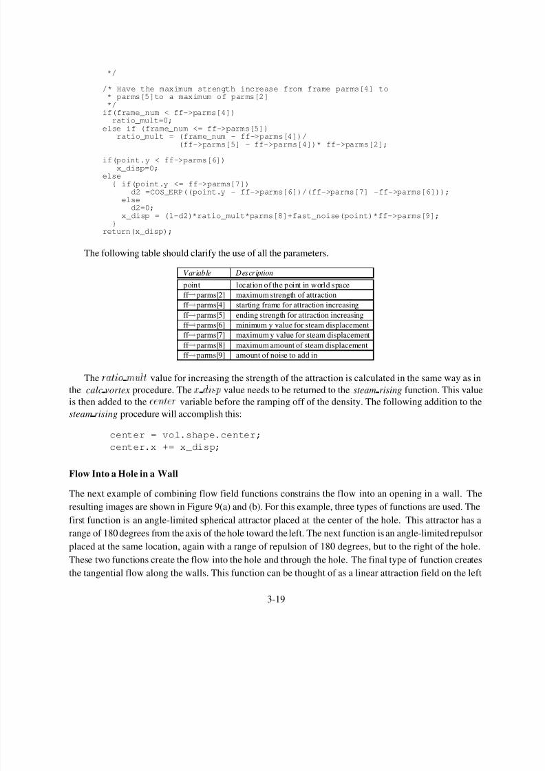
The following table should clarify the use of all the parameters.

Variable Description

point location of the point in world space

ff ! parms[2] maximum strength of attraction

ff ! parms[4] starting frame for attraction increasing

ff ! parms[5] ending strength for attraction increasing

ff ! parms[6] minimum y value for steam displacement

ff ! parms[7] maximum y value for steam displacement

ff ! parms[8] maximum amount of steam displacement

ff ! parms[9] amount of noise to add in

Ther a t i o m u l t

value for increasing the strength of the attraction is calculated in the same way as in

the calc vortex procedure. Thex d i s p

value needs to be returned to the steam rising function. This value

is then added to thec e n t e r

variable before the ramping off of the density. The following addition to thesteam rising procedure will accomplish this:

center = vol.shape.center;

center.x += x_disp;

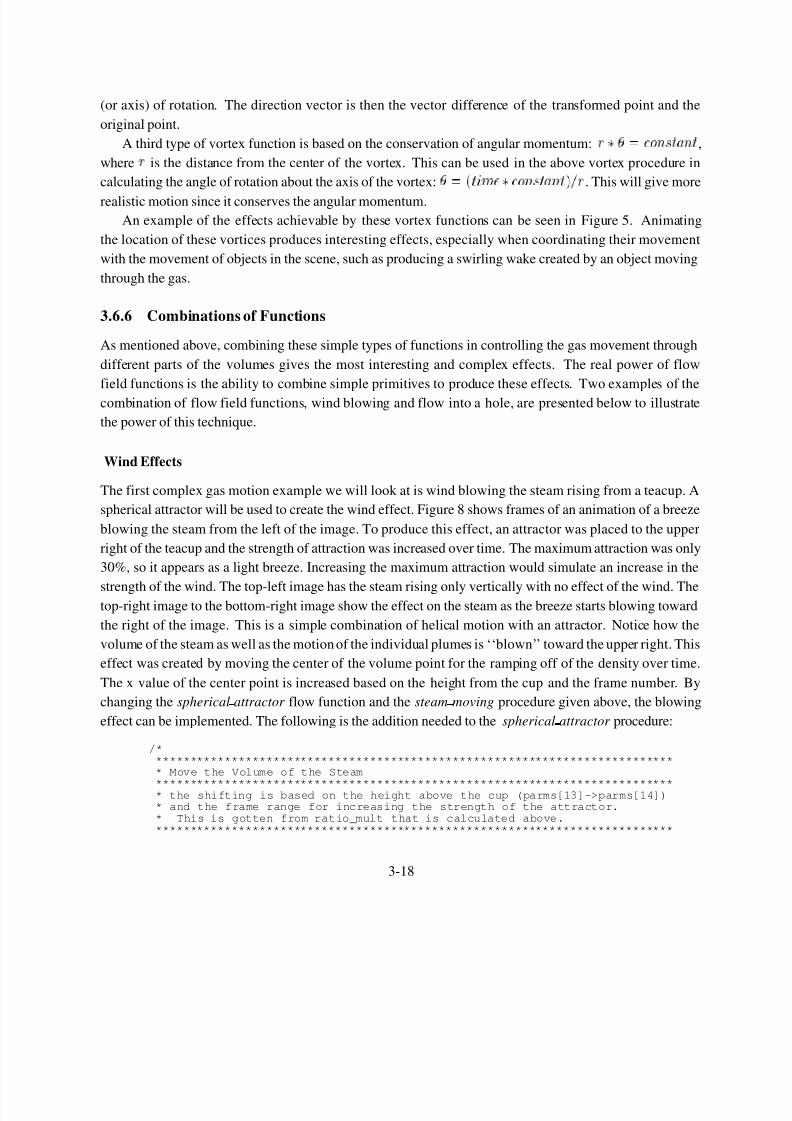
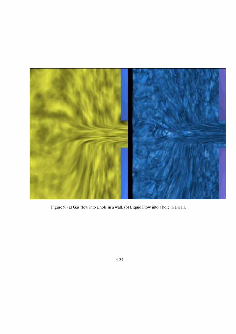
Flow Into a Hole in a Wall

The next example of combining flow field functions constrains the flow into an opening in a wall. The

resulting images are shown in Figure 9(a) and (b). For this example, three types of functions are used. The

first function is an angle-limited spherical attractor placed at the center of the hole. This attractor has a

range of 180 degrees from the axis of the hole toward the left. The next function is an angle-limited repulsor

placed at the same location, again with a range of repulsion of 180 degrees, but to the right of the hole.

These two functions create the flow into the hole and through the hole. The final type of function creates

the tangential flow along the walls. This function can be thought of as a linear attraction field on the left

3-19



side of the hole. The line in this case would be through the hole and perpendicular to the wall(horizontal).

This attractor has maximum attraction near the wall, with the attraction decreasing as you move away from

the wall. As you can see from the flow patterns toward the hole and along the wall in Figure 9, the effect is

very convincing. This figure also shows how these techniques can be applied to hypertextures. The right

image is rendered as a hypertexture to simulate a (compressible) liquid flowing into the opening.

3.7 Animating Hypertextures

All of the animation techniques described above can be applied to hypertextures. The only change needed

is in the rendering algorithm. By using a non-gaseous model for illumination and for converting densities

to opacities, the techniques described above will produce hypertexture images. As mentioned above, an

example of this is Figure 9. The geometry and motion procedures are the same for both of the images in

Figure 9. Two other examples of hypertexture animation will be explored: simulating molten marble and

fire.

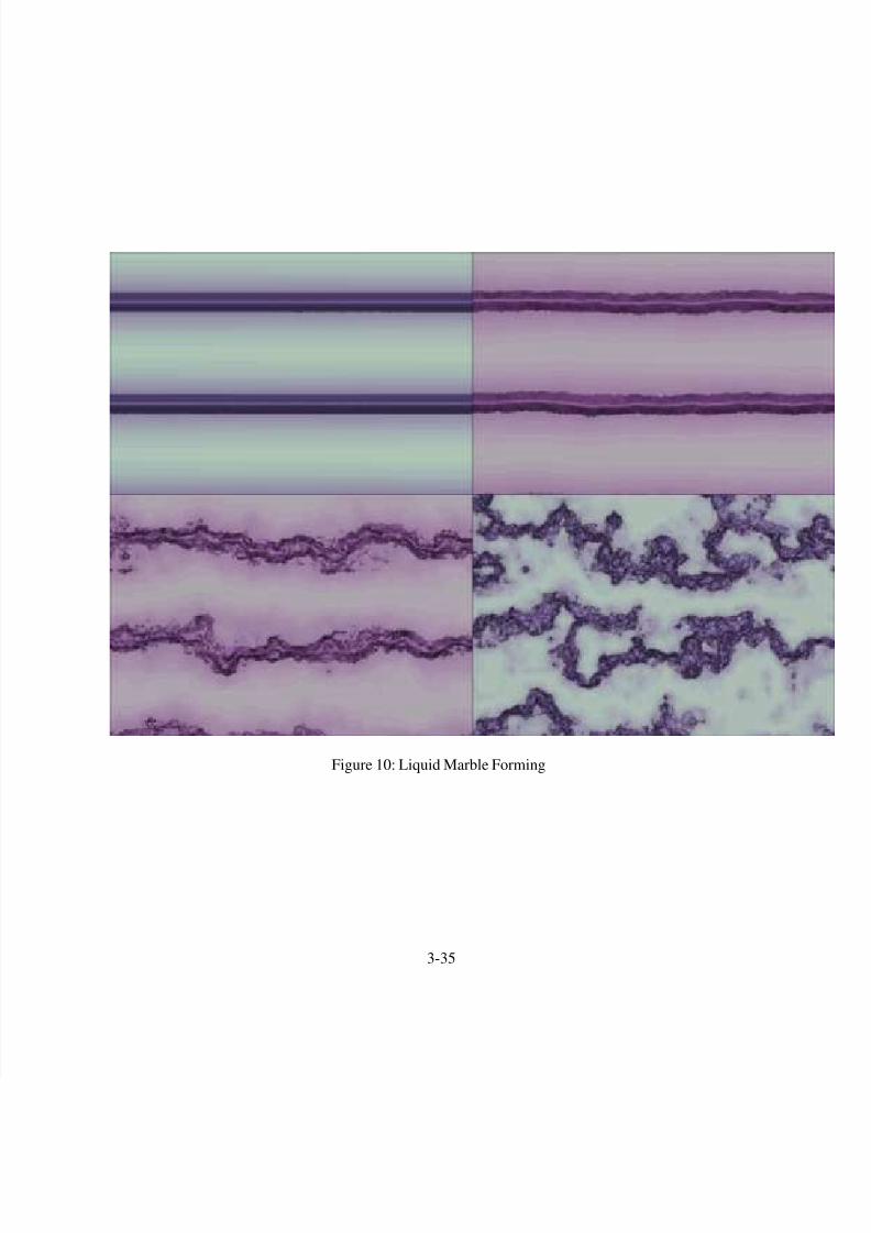
3.7.1 Molten Marble

Previously in these notes, a procedure was given for simulating the formation of marble. The addition of

hypertexture animationto the solid texture animation can increase the realism of the animation considerably.

One way of animating hypertextures for the simulation of marble forming is described below. However,

the reader is encouraged to try various techniques to produce different results.

The main idea behind this approach is to base the density changes on the color of the marble. Initially,

no turbulence will be added to the ‘‘fluid’’: density values will be determined in a manner similar to the

marble color values, giving the different bands different densities. Just as in the earlier marble forming

procedure, turbulence will be added over time. As you can see in the procedure below, all of the above is

achieved by returning the amount of turbulence from the solid texture function, marble forming, described

earlier. The density is based on the turbulence amount from the solid texture function. This is then shaped

using the power function in a similar manner to the gas functions given before. Finally, a trick by Perlin

[17] is used to form a hard surface more quickly. The result of this function can be seen in Figure 10.

/*********************************************************************** parms[1] = Maximum density value: density scaling factor ** parms[2] = exponent for density scaling ** parms[3] = x resolution for Perlin’s trick (0-640) ** parms[8] = 1/radius of fuzzy area for perlin’s trick (> 1.0) ***********************************************************************/

molten_marble(pnt, density, parms,vol)xyz_td pnt;

float *density,*parms;vol_td vol;

{float parms_scalar, turb_amount;

3-20



turb_amount = solid_txt(pnt,vol);*density = (pow(turb_amount, parms[2]) )*0.35 +.65;

/* Introduce a harder surface quicker. parms[3] is multiplied by 1/640 */*density *=parms[1];parms_scalar = (parms[3]*.0015625)*parms[8];*density= (*density-.5)*parms_scalar +.5;*density = MAX(0.2, MIN(1.0,*density));

}

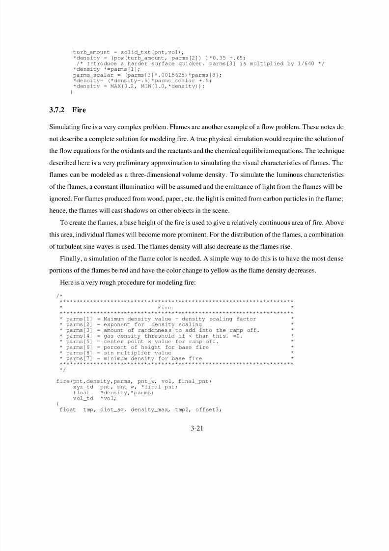
3.7.2 Fire

Simulating fire is a very complex problem. Flames are another example of a flow problem. These notes do

not describe a complete solution for modeling fire. A true physical simulation would require the solution of

the flow equations for the oxidants and the reactants and the chemical equilibrium equations. The technique

described here is a very preliminary approximation to simulating the visual characteristics of flames. The

flames can be modeled as a three-dimensional volume density. To simulate the luminous characteristics

of the flames, a constant illumination will be assumed and the emittance of light from the flames will be

ignored. For flames produced from wood, paper, etc. the light is emitted from carbon particles in the flame;

hence, the flames will cast shadows on other objects in the scene.

To create the flames, a base height of the fire is used to give a relatively continuous area of fire. Above

this area, individual flames will become more prominent. For the distribution of the flames, a combination

of turbulent sine waves is used. The flames density will also decrease as the flames rise.

Finally, a simulation of the flame color is needed. A simple way to do this is to have the most dense

portions of the flames be red and have the color change to yellow as the flame density decreases.

Here is a very rough procedure for modeling fire:

/*********************************************************************** Fire *********************************************************************** parms[1] = Maimum density value - density scaling factor ** parms[2] = exponent for density scaling ** parms[3] = amount of randomnes s to add into the ramp off. ** parms[4] = gas density threshold if < than this, =0. ** parms[5] = center point x value for ramp off. ** parms[6] = percent of height for base fire ** parms[8] = sin multiplier value ** parms[7] = minimum density for base fire ***********************************************************************/

fire(pnt,density,parms, pnt_w, vol, final_pnt)

xyz_td pnt, pnt_w, *final_pnt;float *density,*parms;vol_td *vol;

{float tmp, dist_sq, density_max, tmp2, offset3;

3-21



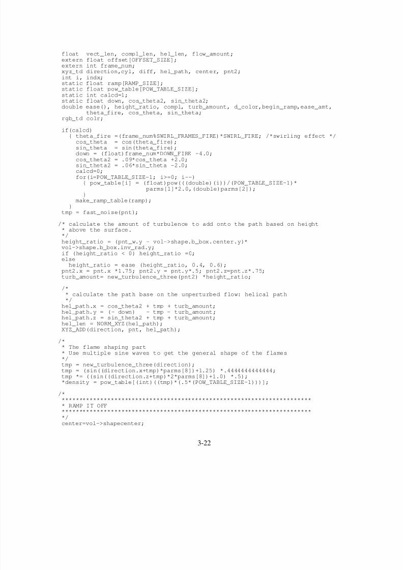
float vect_len, compl_len, hel_len, flow_amount;extern float offset[OFFSET_SIZE];extern int frame_num;xyz_td direction,cyl, diff, hel_path, center, pnt2;int i, indx;static float ramp[RAMP_SIZE];static float pow_table[POW_TABLE_SIZE];static int calcd=1;

static float down, cos_theta2, sin_theta2;double ease(), height_ratio, compl, turb_amount, d_color,begin_ramp,ease_amt,

theta_fire, cos_theta, sin_theta;rgb_td colr;

if(calcd){ theta_fire =(frame_num%SWIRL_FRAMES_FIRE)*SWIRL_FIRE; /*swirling effect */

cos_theta = cos(theta_fire);sin_theta = sin(theta_fire);down = (float)frame_num*DOWN_FIRE -4.0;cos_theta2 = .09*cos_theta +2.0;sin_theta2 = .06*sin_theta -2.0;calcd=0;for(i=POW_TABLE_SIZE-1; i>=0; i--)

{ pow_table[i] = (float)pow(((double)(i))/(POW_TABLE_SIZE-1)*parms[1]*2.0,(double)parms[2]);

}

make_ramp_table(ramp);}

tmp = fast_noise(pnt);

/* calculate the amount of turbulence to add onto the path based on height* above the surface.*/height_ratio = (pnt_w.y - vol->shape.b_box.center.y)*vol->shape.b_box.inv_rad.y;if (height_ratio < 0) height_ratio =0;else

height_ratio = ease (height_ratio, 0.4, 0.6);pnt2.x = pnt.x *1.75; pnt2.y = pnt.y*.5; pnt2.z=pnt.z*.75;turb_amount= new_turbulence_three(pnt2) *height_ratio;

/** calculate the path base on the unperturbed flow: helical path

*/hel_path.x = cos_theta2 + tmp + turb_amount;hel_path.y = (- down) - tmp - turb_amount;hel_path.z = sin_theta2 + tmp + turb_amount;hel_len = NORM_XYZ(hel_path);XYZ_ADD(direction, pnt, hel_path);

/** The flame shaping part* Use multiple sine waves to get the general shape of the flames*/tmp = new_turbulence_three(direction);tmp = (sin((direction.x+tmp)*parms[8])+1.25) *.4444444444444;tmp *= ((sin((direction.z+tmp)*2*parms[8])+1.0) *.5);*density = pow_table[(int)((tmp)*(.5*(POW_TABLE_SIZE-1)))];

/*

************************************************************************ RAMP IT OFF************************************************************************/center=vol->shapecenter;

3-22



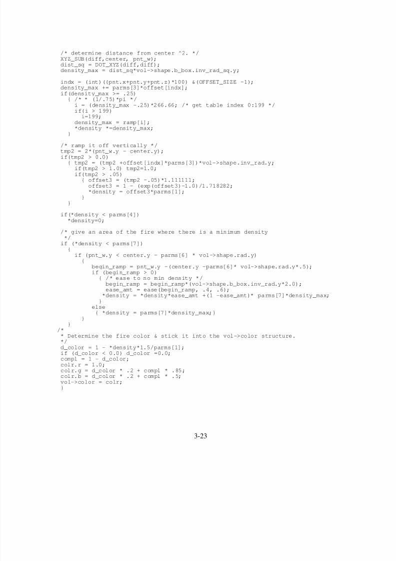
/* determine distance from center ^2. */XYZ_SUB(diff,center, pnt_w);dist_sq = DOT_XYZ(diff,diff);density_max = dist_sq*vol->shape.b_box.inv_rad_sq.y;

indx = (int)((pnt.x+pnt.y+pnt.z)*100) &(OFFSET_SIZE -1);density_max += parms[3]*offset[indx];if(density_max >= .25)

{ /* * (1/.75)*pi */i = (density_max -.25)*266.66; /* get table index 0:199 */if(i > 199)

i=199;density_max = ramp[i];*density *=density_max;

}

/* ramp it off vertically */tmp2 = 2*(pnt_w.y - center.y);if(tmp2 > 0.0)

{ tmp2 = (tmp2 +offset[indx]*parms[3])*vol->shape.inv_rad.y;if(tmp2 > 1.0) tmp2=1.0;if(tmp2 > .05)

{ offset3 = (tmp2 -.05)*1.111111;offset3 = 1 - (exp(offset3)-1.0)/1.718282;*density = offset3*parms[1];

}}

if(*density < parms[4])*density=0;

/* give an area of the fire where there is a minimum density*/

if (*density < parms[7]){

if (pnt_w.y < center.y - parms[6] * vol->shape.rad.y){

begin_ramp = pnt_w.y -(center.y -parms[6]* vol->shape.rad.y*.5);if (begin_ramp > 0)

{ /* ease to no min density */begin_ramp = begin_ramp*(vol->shape.b_box.inv_rad.y*2.0);ease_amt = ease(begin_ramp, .4, .6);

*density = *density*ease_amt +(1 -ease_amt)* parms[7]*density_max;}

else{ *density = parms[7]*density_max;}

}}

/** Determine the fire color & stick it into the vol->color structure.*/d_color = 1 - *density*1.5/parms[1];if (d_color < 0.0) d_color =0.0;compl = 1 - d_color;colr.r = 1.0;colr.g = d_color * .2 + compl * .85;colr.b = d_color * .2 + compl * .5;vol->color = colr;}

3-23



3.8 Conclusion

The goal of these notes has been to describe my techniques to create realistic images and animations of gases

and fluids in detail, as well as provide the reader with an insight into the development of these techniques.

These notes have shown a useful approach to modeling gases and powerful animation techniques forprocedural modeling. A more detailed and expanded description of these techniques can be found in [4]. To

aid the reader in reproducing the results presented here, all of the images in these notes are accompanied by

detailed descriptions of the procedures used to create them. opportunity to reproduce the results, but also

the opportunity and challenge to expand upon the techniques presented in these notes. This gives the reader

not only the These notes should also give the reader an insight into the procedural design approach I use

and will hopefully help the reader explore and expand procedural modeling and animation techniques.

References

[1] Ebert, David, Boyer, Keith, and Roble, Doug. Once a Pawn a Foggy Knight ... [videotape]. InSIGGRAPH Video Review 54 (November 1989), ACM SIGGRAPH, New York. segment 3.

[2] Ebert, David, Carlson, Wayne, and Parent, Richard. Solid Spaces and Inverse Particle Systems forControlling the Animation of Gases and Fluids. The Visual Computer 10, 4 (1994), 179--190.

[3] Ebert, David, Ebert, Julia, and Boyer, Keith. Getting Into Art. [videotape], Department of Computerand Information Science, The Ohio State University, May 1990.

[4] Ebert, David, Musgrave, F. Kenton, Peachey, Darwyn, Perlin, Ken, and Worley, Steve. Texturingand Modeling: A Procedural Approach. AP Professional, Boston, MA, 1994.

[5] Ebert, David, and Parent, Richard. Rendering and Animation of Gaseous Phenomena by CombiningFast Volume and Scanline A-buffer Techniques. Proceedings of SIGGRAPH’90,(Dallas, Texas, Aug

6-10, 1990 ). In Computer Graphics 24,4 (August 1990), 357--366.[6] Ebert, David, Yagel, Roni, Scott, Jim, and Kurzion, Yair. Volume Rendering Methods for

Computational Fluid Dynamics Visualization Proceedings of Visualization ’94. 232--239.

[7] Ebert, David S. Solid Spaces: A Unified Approach to Describing Object Attributes. PhD thesis, TheOhio State University, 1991.

[8] Gardner, Geoffrey. Visual Simulation of Clouds. Proceedings of SIGGRAPH’85 (San Francisco,California, July 22-26, 1985). In Computer Graphics 19,3 (July 1985), 297--303.

[9] Gardner, Geoffrey. Forest Fire Simulation. Proceedings of SIGGRAPH’90, (Dallas, Texas, Aug 6-10,1990 ). In Computer Graphics 24,4 (August 1990), 430.

[10] Inakage, Masa. Modeling Laminar Flames. In SIGGRAPH’91: Course Notes 27 (July 1991), ACMSIGGRAPH.

[11] Kajiya, James, and Von Herzen, Brian. Ray Tracing Volume Densities.Proceedings of SIGGRAPH’84(Minneapolis, Minnesota, July 23-27, 1984). In Computer Graphics 18,3 (July 1984), 165--174.

3-24



[12] Kay, Timothy, and Kajiya, James. Ray Tracing Complex Scenes. Proceedings of SIGGRAPH’86(Dallas, Texas, August 18-22, 1986). In Computer Graphics 20, 4 (August 1986), 269--278.

[13] Klassen, R. Victor. Modeling the Effect of the Atmosphere on Light. ACM Transaction on Graphics6 , 3 (July 1987), 215--237.

[14] Max, Nelson. Light Diffusion Through Clouds and Haze. Computer Vision, Graphics, and Image

Processing 33 (1986), 280--292.[15] Nishita, Tomoyuki, Miyawaki, Yasuhiro, and Nakamae, Eihachiro. A Shading Model for Atmo-

spheric Scattering Considering Luminous Intensity Distribution of Light Sources. Proceedings of SIGGRAPH’87 (Anaheim, California, July 27-31, 1987). In Computer Graphics 21,4 (July 1987),303--310.

[16] Perlin, Ken. An Image Synthesizer. Proceedings of SIGGRAPH’85 (San Francisco, California, July22-26, 1985). In Computer Graphics 19,3 (July 1985), 287--296.

[17] Perlin, Ken. A Hypertexture Tutorial. In SIGGRAPH’92: Course Notes 23 (July 1992), ACMSIGGRAPH.

[18] Perlin, Ken, and Hoffert, Eric. Hypertexture. Proceedings of SIGGRAPH’89, (Boston, Massachusetts,July 31-Aug 4, 1989 ). In Computer Graphics 23,3 (July 1989), 253--262.

[19] Sims, Karl. Particle Animation and Rendering Using Data Parallel Computation. Proceedings of SIGGRAPH’90 (Dallas, Texas, Aug 6-10, 1990 ). In Computer Graphics 24,4 (August 1990),405--413.

[20] Stam, Joe, and Fiume, Eugene. Turbulent Wind Fields for Gaseous Phenomena. Proceedings of SIGGRAPH’93 (Anaheim, California, August 1-6, 1993). In Computer Graphics, Annual ConferenceSeries, 1993 (August 1993), 369--376.

[21] Voss, Richard. Fourier Synthesis of Gaussian Fractals: 1/f noises, landscapes, and flakes. InSIGGRAPH 83: Tutorial on State of the Art Image Synthesis (1983), vol. 10, ACM SIGGRAPH.

[22] Wyvill, Brian, and Bloomenthal, Jules. Modeling and Animating with Implicit Surfaces. InSIGGRAPH 90: Course Notes 23 (August 1990), ACM SIGGRAPH.

3-25



Figure 1: The effects of the power and sine function on the gas shape. (a) has a power exponent of 1, (b)

has a power exponent of 2, (c) has a power exponent of 3, and (d) has the sine function applied to the gas.

3-26



Figure 2: Solid textured transparency based fog.

3-27



Figure 3: Marble forming. The images show the banded material heating, deforming, then cooling and

solidifying.

3-28



Figure 4: Effect of a spherical attractor increasing over time. Images are every 45 frames. The top-left

image has 0 attraction. The lower-right image has the maximum attraction.

3-29



Figure 8: A increasing breeze blowing towards the right created by an attractor.

3-33



Figure 9: (a) Gas flow into a hole in a wall. (b) Liquid Flow into a hole in a wall.

3-34



Figure 10: Liquid Marble Forming

3-35

d.ebert_procedural modeling, animation, and rendering of gases, fluids, and textures

Documents