See discussions, stats, and author profiles for this publication at: https://www.researchgate.net/publication/220792067

Precise vector textures for real-time 3D rendering

Conference Paper · January 2008

DOI: 10.1145/1342250.1342281 · Source: DBLP

CITATIONS

30READS

1,908

3 authors, including:

Some of the authors of this publication are also working on these related projects:

RapidMind/ArBB View project

Zhipei Qin

Apple Inc.

8 PUBLICATIONS   212 CITATIONS   

SEE PROFILE

Michael D. Mccool

Intel

99 PUBLICATIONS   2,309 CITATIONS   

SEE PROFILE

All content following this page was uploaded by Michael D. Mccool on 31 January 2014.

The user has requested enhancement of the downloaded file.

Precise Vector Textures for Real-Time 3D Rendering

Zheng Qin∗

University of WaterlooMichael D. McCool†

University of Waterloo and RapidMind, Inc.Craig Kaplan‡

University of Waterloo

Figure 1: A scene using several vector textures with some closeups showing embossing and transparency.

AbstractVector graphics representations of images are resolution indepen-dent. Direct use of vector images for real-time texture mappingwould be desirable to avoid sampling artifacts such as blurringcommon with raster images. Scalable Vector Graphics (SVG) filesare typical of vector graphics image representations. Such repre-sentations composite images from layers of paths and strokes de-fined with lines, elliptical arcs, and quadratic and cubic parametricsplines.

High-quality texture mapping requires both random access andanisotropic antialiasing. For vector images, these goals can beachieved by computing the distance to the closest primitives from asample point and then mapping this distance through a soft thresh-old function. Representing transparency masks in this way is es-pecially useful, since vector mattes can be used to render complexcurvilinear geometry as textures on simple geometric primitives.

Unfortunately, computing the exact minimum distance to theparametric curves used in vector images is difficult. Previous workhas used approximations, but an accurate minimum distance is de-sirable in order to enable wide strokes and special effects such asembossing. In this paper, a simple algorithm is presented that canefficiently and accurately compute the minimum distance to a para-metric curve when the sample point is within its radius of curva-ture and the curve can be segmented into monotonic regions. Thistechnique can be used in a GPU shader to render antialiased vectorimages exactly as defined by SVG files.

CR Categories: I.3.7 [Computer Graphics]: Three-DimensionalGraphics and Realism—Color, shading, shadowing, and texture

Keywords: vector graphics, antialiasing, texture, distance to cubicspline curves.

∗e-mail: zqin@uwaterloo.ca†e-mail: mmccool@uwaterloo.ca or mmccool@rapidmind.com‡e-mail: cskaplan@uwaterloo.ca

1 IntroductionThe world around us teems with text, ornamentation, and othersymbolic surface patterns with sharp edges. As we move closeto them, these sharp edges remain sharp. Raster texture maps, theusual means of decorating surfaces in computer-generated imagery,do not have this property. As we zoom in to a textured surface, thesurface detail starts to appear blurred or pixelated when we run outof resolution in the underlying texture map. We would like to cre-ate a representation of a vector image that allows it to be used likea texture map, but which looks sharp at any resolution.

Recent research has attempted to address the limitations of stan-dard raster images by providing direct support for some form ofvector data during texture mapping. These approaches, which arereviewed in detail in the next section, fall into two main categories:approximate and exact techniques. In either case, in order to sup-port texture mapping the representation must support efficient ran-dom access. Anisotropic antialiasing that can tolerate image warp-ing is also necessary for high quality results.

Approximate techniques limit the generality of the vector im-ages supported, or accept reduced image quality in exchange for in-creased performance. Example tradeoffs of approximate techniquesinclude rounded corners, limited maximum complexity in a region,limited color support (for example, a restriction to bi-level images),and finally support for only a limited set of curve primitive types(for example, only line segments).

In contrast, exact techniques render content exactly as expressedin a standard vector image format such as SVG. The advantage ofimporting images expressed in a standard representation is that ex-

isting vector graphics tools can be used to edit the content, and sup-porting the full generality of these tools gives the artist maximumflexibility.

Unfortunately, SVG and related file formats (such as PDF) rep-resent boundaries with parametric curves and higher-order splines,which complicate color retrieval and antialiasing. Fast random ac-cess and high quality antialiasing require an augmented representa-tion. Such augmented representations typically combine an accel-erator structure that limits the boundary features to be consideredfor every access with a representation of those features that enablesefficient antialiasing.

Our results contribute to this second category of research. Wecompute the exact geometry in the vector image as represented inthe SVG file, and render it with high-quality antialiasing.

We use the signed distance to the closest boundary feature as animplicit representation of that feature [Frisken et al. 2000]. Oncecomputed, the signed distance function can be mapped through asmooth step to obtain a blending function for antialiasing, and thegradient can be used to modulate the width of the transition to ob-tain anisotropic antialiasing [Qin et al. 2006]. The distance can alsobe used to render strokes of a precise width and to implement spe-cial effects such as embossing.

The boundaries in standard vector graphics file formats such asSVG may include points, line segments, elliptical arcs, and splinecurves. We refer to these boundary elements as features. Of thesefeatures, cubic spline curves are the most complex. Unfortunately,computing the distance to higher-order parametric spline curves di-rectly is expensive.

The main contribution of this paper is a simple, robust, and prac-tical way to compute the accurate distance to any curved featurefrom a sample point within its radius of curvature. In particular,higher order parametric spline curves do not need to be approxi-mated by lower order polynomials, so that the original smoothnessof the boundary is retained. One of the main applications of accu-rate distance field gradients is embossing; as a secondary contribu-tion we also present a technique for second-order antialiasing of theridge lines that can appear during embossing.

2 BackgroundModified interpolation rules for hybrid vector/raster images havebeen proposed that support up to four linear discontinuities in ev-ery pixel [Sen et al. 2003; Sen 2004; Tumblin and Choudhury2004]. These representations were implemented in real time inGPU shaders and could even be generated on the GPU. However,in these representations the linear discontinuities had to go throughopposite edges of each cell, so many line drawings could not berepresented exactly. Antialiasing was also not considered.

In cell-based representations only some cells contain edges, en-abling a sparse representation. An implementation of antialiased bi-level vector images was demonstrated using perfect spatial hashingfor sparse storage [Lefebvre and Hoppe 2006], using two arbitrarilyoriented linear edges per pixel.

Cell-based storage with clipped parametric primitives has alsobeen used [Ramanarayanan et al. 2004], again with modified rulesfor raster sample interpolation. This work used a spatial data struc-ture that could represent an arbitrary number of parametric cubicboundaries in every cell, and so could support general SVG fileswith arbitrary complexity. Subdivision into monotonic regions al-lowed robust numerical evaluation of exact cubic boundaries, butthe data structure was not implemented in real time on the GPU.

Implicit functions have been used to represent curved disconti-nuities within a cell. These can be combined with Boolean opera-tions to support more complex combinations of features in a cell, in-cluding sharp corners [Ray et al. 2005]. This work also introducedsprite tables for dynamic layout of text. However, low-order im-plicit functions can only approximate the curved parametric primi-

tives used in SVG files.One of the limitations of fixed-size cell-based approaches is the

limited complexity that can be supported in any one region. Warp-ing of the grid can be used to overcome this limitation to someextent [Tarini and Cignoni 2005].

Analytic evaluation of implicit functions can be used to representexactly all the primitives supported by SVG. In particular, exact im-plicit forms of parametric cubics can be computed [Loop and Blinn2005]. Dividing these implicit forms by the magnitude of their gra-dient gives a function that is similar to the distance function close tothe boundary and can be used for antialiasing. However, paramet-ric curves represent only a segment of a cubic, while implicits givethe entire curve. Therefore it is necessary to limit the domains overwhich these implicit forms are evaluated to avoid phantom edges.

Another approach that can render SVG vector images as texturemaps uses a cellular structure, but with an arbitrarily complex “texelprogram” per cell [Nehab and Hoppe 2007]. The texel programcan represent all paths affecting that cell and layer them in SVGdrawing order. This system runs in real time on the GPU, but usesan implicit form that limits it to segments of quadratic parametriccurves. Cubic parametric curves in the input are approximated.

Thresholding of signed distance fields can be used as a gen-eral implicit representation of bi-level images and volumes [Friskenet al. 2000]. If adaptive resolution is used, sharp corners canbe represented, and antialiasing can be implemented using simplesmooth-step thresholding. If uniform sampling is used, sharp cor-ners cannot be exactly reconstructed, but this limitation is accept-able in some applications, since this representation is nearly as fastas ordinary texturing [Green 2007]. It is, however, possible to sup-port adaptive resolution on GPUs [Kraus and Ertl 2002; Lefebvreand Hoppe 2007]. Also, the distance samples in the texture can bemodified by optimization so the bilinear interpolation supported inhardware is a better fit to the vector outlines [Loviscach 2005].

Exact computation of the minimum signed distance to line seg-ments has been used for bi-level images, in particular font tables,using a cell-based representation based on packing and local search[Qin et al. 2006]. This work also presented a scheme for supportingapproximate anisotropic antialiasing, which is especially importantfor maintaining the readability of text, and used a sprite map for dy-namic text layout. The use of exact distance computations permitsspecial effects such as outlining and embossing.

In order to support the cubic parametric curves found in SVGfiles together with these special effects, an exact distance compu-tation is desirable. Unfortunately, computing the exact distancefrom a point to a cubic curve is difficult, since it involves find-ing the roots of a degree 5 equation [Wang et al. 2002; Plass andStone 1983; Johnson and Cohen 2005]; even finding distances toquadratic curves is hard.

Compared to previous work, our representation is the first thatcan handle all the curved primitives in SVG files, including cubicsand elliptical arcs, exactly and in real time. We can also renderthese paths with special effects such as outlining and embossing.

3 AlgorithmOur approach has two parts: a preprocessed representation that em-beds the vector image in a set of texture maps, and an algorithmimplemented in a shader for interpreting this information to com-pute the color of the vector image at any point. The representationmust support fast access to the minimum amount of data at everypoint. The basis of the color computation is a fast distance compu-tation.

In order to build our representation, a uniform grid is first su-perimposed on the vector image. Each cell is checked against theboundary features to find the subset of features that intersect it. Allboundary features that intersect a cell are stored in a per-cell list.This list is then augmented by features within a certain distance of

the cell to support antialiasing; the extension distance is boundedby using MIP-maps in the far field.

Color retrieval and boundary antialiasing for any point in a cellneed only consider the cell’s feature list. As mentioned above, thedistance to the closest boundary feature is used for antialiasing, andthe gradient of this function is used for anisotropic antialiasing.

We will talk about how to build the representation in Section 3.1and then how to compute the distance and use it for antialiasing inSection 3.2.

3.1 PreprocessingA typical SVG image is composed of closed paths or strokes. Pathscan have borders of various widths and colors, and can be orientedin either a clockwise or counter-clockwise direction. The regionenclosed by a path can be filled with a solid color or a gradient.Strokes may also have colors and widths. For now we will only dealwith filled paths without border colors, but will discuss generaliza-tions in a later section. We also assume the images only containclosed simple paths oriented in a counter-clockwise fashion, andthat these paths do not cross themselves. If a path crosses itself, itshould be separated into multiple simple paths [Eigenwillig et al.2006].

To build our representation, we first split curves into monotonicsegments, which will simplify the distance computation later. Wethen index these feature segments with an accelerator structure thatallows fast random access lookup of the features needed during ren-dering.

3.1.1 Splitting Curves

Figure 2: (a) All curves are split into C and S shaped features atevery point where the tangents are horizontal or vertical. (b) Thebounding box of a path is the bounding box of its features.

In order to simplify the distance computation, we split each curveat the points where its tangent is horizontal or vertical. For example,in Figure 2(a), the given spline is split into four segments at the reddots. Let the parametric form of the curve be given by P (u) =[x(u), y(u)]. For cubic splines, the splitting points u∗ can be foundby solving for the roots of the quadratic parametric splines givingthe components of the tangent ~T (u) = [x′(u), y′(u)] of P (u):

x′(u∗) = 0 or y′(u∗) = 0.

There are at most four split points, as there are at most two solutionsfor each of the above equations, so curves are broken into at mostfive segments.

Each resulting segment has a simple shape. In fact, after splittingthere are only two categories of shape, as shown in figure 2(a). Wecall these categories C-shapes and S-shapes. Note that over eachsegment, x′(u) and y′(u) are either completely positive or nega-tive. We call such functions monotonic. The C-shape represents allcurves with no inflection point. The S-shape represents all curveswith one inflection point. Since the second derivative of a cubicis a linear function, there can be at most two such points: one for

x′′(u∗) = 0 and one for y′′(u∗) = 0. We could further split the S-shape into C-shapes at these roots. However, since S-shape curvesstill work with our distance algorithm, we keep them as they are.

Finding the splitting points for (rotated) elliptical arcs andquadratics is similar. Line segments do not have to be split. Aftersplitting, spline curves and elliptical arcs are still spline curves andelliptical arcs. The overall continuity and shape of the boundariesdoes not change.

3.1.2 Detection of Features Overlapping a Cell

In order to build our accelerator structure, a uniform grid of cellsis superimposed on the vector image. For each cell we would liketo find which paths completely contain the cell and which pathsintersect it.

For every cell this process is done path by path in drawing order.Rendering order is important in vector images and as part of thepreprocessing we also need to resolve visibility (and exploit it whenpossible to remove hidden paths).

To accelerate this procedure, the axis-aligned bounding box ofeach path is computed. If a cell does not overlap the bounding boxof a path, the path cannot cover the cell or cross the cell bound-ary at all. Recall that all curves are split into monotonic segments.Because all our split features are monotonic, each one’s boundingbox can be constructed from its two end points. The bounding boxfor an entire path can be computed from the bounding boxes of itsfeatures, as shown in Figure 2(b).

If a path’s bounding box overlaps a cell, all features of the pathare checked against the cell. Our monotonic features can be in-tersected with the four boundary lines of the cell using classicalnumerical methods. If a feature intersects any boundary or if it iscompletely contained by the cell, it is stored in the cell’s list.

If none of the features in a path overlaps a cell, two situationsare possible. The path can be outside the cell or it can completelycontain it. In the latter case, all features that are already listed forthe cell are deleted, and the background color of the cell is set to thefill color of the current path. All previous features will be coveredby the new path.

We use the winding rule to test if a cell is contained by apath [Nehab and Hoppe 2007]. Any point in the cell can be chosenfor the test; we choose the lower left corner of the cell.

3.1.3 Cell Extension

When the path is checked against a cell, the cell extent needs tobe expanded to tolerate some level of texture minification. The an-tialiasing filter will have a certain width in texture space, and weneed to be able to compute distances to at least this width. Themagnitude of the expansion depends on the level of image minifi-cation to be supported during vector rendering.

At higher minification levels, texture rendering should be im-plemented with a raster-based MIP-map. This raster image can berendered (on the GPU) directly from the vector texture. Under mini-fication MIP-mapping gives an accurate antialiased representationof the vector image, and transitions can be managed using the al-pha channel of the raster texture. The finest resolution raster imageshould be stored with α = 0, the other coarser levels should useα = 1. Then trilinear interpolation of α will give the correct valuefor blending between raster and vector rendering. Vector render-ing can be disabled using control flow in the shader when α = 1.If the texture includes transparency, then the shader can computethe transition function explicitly using the Jacobian of the texturecoordinate to screen space mapping.

However, extending the cell by a fixed amount may not includeall features needed to compute the inside/outside test correctly. Theextension width should be chosen so that if a feature crossing thecell is included, all features that might be closer for any point in thecell should also be included.

3.1.4 Acceleration Structure

At this point, have a list of relevant features and the backgroundcolor for each cell. This information needs to be stored in an accel-eration structure. We use three textures to store this information inan efficient way.

Figure 3: Three textures are used to store the accelerator structure.

At the lowest level we list all features from all paths, includingpoints, line segments, quadratic splines, cubic splines, ellipses, andso on in one texture. Each feature is stored only once. The featuresare grouped and sorted according to paths. Features belonging tothe same path are put together with a header that stores per-pathinformation, such as fill color, border color, border width, etc. Thistexture is shown in Figure 3(c).

Next, for each cell, the list of features that crosses this cell aresorted according to the paths they belong to. For example, supposethere are several features from two paths that overlap the cell. Somebelong to the first path, and some belong to the second path. Thenthe features belonging to the first path are grouped together, as arethe features belonging to the second path. Just before the list offeatures in each path, an extra storage slot is used to record thenumber of features used. This texture stores pointers into the low-level texture that refer to the features used. Thus only one storageslot is needed for each feature. This stage is shown in Figure 3(b).

The final texture is a grid texture corresponding to the cells. Foreach cell it holds the start location of the list of features in the sec-ond texture. The corresponding list of features are exactly those thatoverlap the cell. It also stores the number of paths that go throughthis cell, and the background color for the cell. If two cells haveidentical feature lists, they share a single list in the list texture de-scribed above. Figure 3(a) gives an example, including two cellsthat share a feature list.

3.2 Shader ComputationThe shader computation accesses the accelerator to determine thefeatures that need to be considered for each cell. Each path isconsidered in sequence and its color composited to create the finalcolor. First we will consider how inside/outside testing for a path iscomputed and how compositing is performed, then will discuss thedetails of how the distance to a feature is computed.

3.2.1 Path Compositing

The order of the paths and feature lists in every cell needs to beconsistent with the input order in the SVG file. We start with thebackground color and the list of paths and features for the cell. Thesigned distance to the closest feature in every path is computed insequence. For every path, the sign is used to find if the test point

is inside or outside that path. A point is inside a path if it is on theright side of the closest feature and in this case we use a negativedistance. The closest distance of each new path may have the sameor a different sign from the previous one, and may also be smalleror larger in magnitude.

We always keep track of the distance d with the smallest mag-nitude, a foreground color F , and background color B. These twocolors are always the colors on each side of the closest boundary.Suppose D is the closest signed distance to the next path in thesequence and C is its fill color. We update d, F , and B as follows:

bool q = D < 0 or |D| < |d|;bool p = q and d < 0;B = p ? F : B;F = q ? C : F ;d = q ? D : d;

At the end of the process, the distance value with the smallest mag-nitude and its sign are used to find the antialiasing blend weightsusing a smooth step, with the transition width found using the Ja-cobian of the texture coordinate transformation [Qin et al. 2006].Some extensions are required to handle strokes, borders, gradients,and so forth; these are discussed in a later section.

Figure 4: Inside/outside test errors at the corners.

When a signed distance is used to detect if a point is inside oroutside a path, an ambiguity is possible at sharp corners. In Fig-ure 4, a closed path is represented by the green shape. Lines be andea are tangent at the corner e. The directions of these lines are con-sistent with the direction of the path contour. For any point that fallsinside the gray shaded area, its closest distance to the path boundaryis the distance to the corner. In this figure, the closest distance ofpoint p to the path is pe. As the two closest distances are the same,the simple minimum distance rule randomly choses either line beor line ea for the inside/outside test. The sign is computed by pro-jecting pe onto a 90 degree rotation of the corresponding tangent.However, only tangent be gives the correct sign. This problem hasbeen described in [Qin et al. 2006]; to resolve this issue, they intro-duce a small gap in the contour. Instead, we compute the distancefrom p to the extended tangent lines eb and ea and choose the fea-ture that has the larger absolute value to these lines in case of a tieon the minimum distance.

3.2.2 Distance Computation

The core of our algorithm is the computation of the signed distanceto a feature. The distance computation to a line segment is sim-ple, and has been described elsewhere [Qin et al. 2006]. However,the distance computation to a quadratic or cubic spline or an el-liptical arc is not as straightforward. We present an approach todistance computation based on binary search and can be applied toany kind of parametric curve. This approach is fast and simple, butonly accurate when the query point is within the curve’s radius of

curvature. However, the correct sign is always achieved and theresult is sufficiently accurate that images with high visual qualitycan be achieved. There are a few cases where the lack of accuracycan cause problems; after describing the algorithm we will discussthese in detail.

Figure 5: The closest point on a curve to an arbitrary point p canbe found using a binary search based on normal line tests. In re-gions where normal lines cross, the binary search algorithm mayfail, but normal lines only intersect each other beyond the smallestradius of curvature.

We first bound the parametric location of the closest point onthe curve using an interval that contains the entire curve segment.At each iteration, the interval is split at its parametric midpoint.We then extend the normal at the the splitting point into a splittingplane, as shown in figure 5. The point is tested against this plane.The half curve that is on the same side of the plane as the pointis chosen for the next iteration. Iterations can be repeated until acertain error tolerance is reached or for a fixed number of iterations.

Figure 6: The normal lines for C-shaped and S-shaped curves donot intersect the curve itself again.

To understand the properties of this algorithm, first observe forC-shapes and S-shapes the normal lines always intersect the curveexactly once; see Figure 6(a),(b). Case (c) does not occur since wehave split the curves. Second, observe that if we draw two normallines at any two points on the curve, the normal lines will neverintersect on the convex side of the curve. However, they always in-tersect on the concave side, but at a distance that is always greaterthan the smallest radius of curvature of the curve. Therefore, for allpoints on the convex side and for points within the radius of cur-vature on the concave side, the normal lines impose a sequentialordering on the space around the curve. Our binary search locatesthe query point’s position in this order. However, beyond the ra-dius of curvature on the concave side the normal lines fold over and

the ordering is lost, so the algorithm may fail. Failures return an-other point on the curve and a distance that may be larger than theminimum, but never smaller.

In all the examples used in this paper, despite the possibility forfailure, no obvious visual errors were observed. This is because forantialiasing, the query points where the distance matters are veryclose to the boundary features, well within the radius of curvaturein all features in our sample images.

Figure 7: Distance computation errors occur for points whose dis-tance to the curve is larger than the curvature radius. In the worstcase this can lead to errors in inside/outside classification.

In embossing, errors will only be visible if the embossing widthis relatively large. To demonstrate the visual appearance of theseerrors, we increased the embossing width in an example until an er-ror was visible. This is shown in Figure 7(a). Since some points donot compute the correct shortest distance, there are some disconti-nuities along the embossed edge.

We considered using other iterative methods to improve the con-vergence of the distance computation. The Newton-Raphson algo-rithm converges quadratically, but it is not guaranteed to converge,and can fail catastrophically. The regula falsi algorithm is guaran-teed to converge given a monotonic region. However, it is hard tosplit general curves into monotonic regions for the distance functionfor all points in a cell. In particular, for a general non-linear curvewe can always find two points on the curve with normal lines thatintersect at some point. This intersection point has two local ex-tremal distances, so at least for this intersection point, the distancefunction is not monotonic, and the regula falsi algorithm cannot beapplied. Basically, this approach would have the same problems asthe binary search algorithm. Furthermore, the evaluation of binarysearch is simpler, since it only involves averaging and not divisionas in regula falsi (or Newton-Raphson).

When the distance of point to the curve is larger than the em-bossing width, it does not matter if the distance is correct or not,since it is not involved in antialiasing or embossing. The sign ofits distance however is always correct, so the inside/outside test, ingeneral, should have no problem. However, some errors may hap-pen at corners. In Figure 4, when a point p is in the gray shadedregion it has equal distances to both curve features. Recall that weuse the distance to the extended tangent line to break a tie. Butif the distance is wrong, and the two distances are not equal, thefeature with the shorter distance will always be chosen. This fea-ture could be the wrong feature, thus generating an inside-outsideclassification error.

Fortunately, this problem is easy to fix. Observe that the errorsonly happen for the points that are in the gray shaded areas. Thereal closest distance should be the distance to the end points. Thedistance to the two end points of any feature are therefore alwayscomputed, and the shortest of the these two and the value computedby binary search is chosen as the final distance.

A problem can also occur if a shape is very thin, and two bound-ary features are very close, and when the test point is far away rel-ative to the curvature radius, and the query point is on the concaveside of the curve. In this specific circumstance, the closest distancesto these two features are not guaranteed to be accurate, and if thedistance to the closer feature is computed incorrectly to be largerthan the distance to the farther feature, the inside/outside test maybe incorrect. This error can however be avoided if the grid spacingis less than the minimum curvature radius. In our examples, weused a relatively large grid spacing, and yet did not have this error,so it may happen only rarely in real images. However, to demon-strate this issue we designed the test case shown in Figure 7(b). Asmall classification error is visible in the lower left of this image;we have circled it in red.

3.2.3 Ridge Antialiasing

Figure 8: (a) Two close edges can cause aliasing along a ridge. (b)Computing the two closest features for each point, and blending thetwo normals will remove this alias.

If two features from the same embossed path are so close thatthe distance between them is smaller than the embossing width, theinteraction of the two embossed regions will cause aliasing along aridge as shown in Figure 8(a). This is because the closest distanceto the two features have different directions, and therefore, differ-ent normals for shading. When they meet, the normals will switchdirection suddenly, causing an aliasing artifact. To solve this prob-lem, for each point, the two closest distances and their correspond-ing shading normals are computed. These two normals are thenblended smoothly at the places where the two distances are nearlyequal. The result is shown in Figure 8(b), where this form of mag-nification aliasing has been resolved. Embossing itself, like otherforms of bump and normal mapping, can still suffer from highlightaliasing under minification. This is visible in some of our test im-ages and needs to be addressed separately, using modification of theembossing depth and shading model with distance.

4 Extensions and ApplicationsUntil now, we have discussed vector images containing only closedpaths, solid fill colors, and with no borders. Our algorithm can beeasily extended to support other rendering styles. We describe afew of these extensions here.

To support closed paths with boundaries, extra space is neededto store boundary widths and colors in the texture. Then, for eachpoint, after the closest distance d is obtained, it is shifted by half ofthe boundary width W towards the outside of the path, for instance,d′ = d − W/2 as in Figure 9(a). After shifting, the fill color andthe boundary color can be blended smoothly at d′ = −W . Themodified distance value and the blended color can also be used toupdate the closest feature and blending colors between paths.

To support strokes with specific stroke colors and widths, the

Figure 9: The distances are modified to support borders(a) andstrokes(b)

closest distance also needs to be modified using d′ = (|d| <W/2)? − |d| : |d| − W/2, as shown in Figure 9(b). This treatsthe strokes as closed paths, and the stroke color as the fill color.This modified distance and stroke color are used during layer com-positing.

The modified distance is only used in color testing. For em-bossing, the embossing valley should be located where the originaldistance is zero.

We did not implement gradient fills in our test system, but theyare a straightforward modification of the fill color computation. Asbefore, extra space to record the gradient coefficients would beneeded. Then instead of using a solid color directly for the fill,the color for any point inside a path would be computed from thegradient coefficients and used in place of the solid color for the re-gion.

Finally, some more interesting extensions are possible. The bi-nary search computes not only the signed distance to each feature,but also the position along each feature which is closest to the querypoint. This defines a 2D coordinate system in the neighbourhoodof the edge. The distance and the parametric value could be usedtogether as texture coordinates to render textured strokes, wherethe texture could either be a raster texture or another vector tex-ture. This could also be used to implement dashed and dotted linesprocedurally. It would also be possible to permit the specificationof programmable functions for the embossing profile, and use thedistance for other purposes, such as drop shadows.

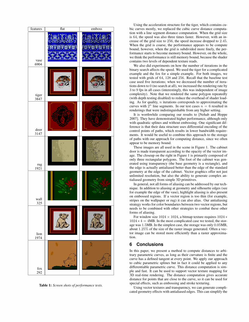
5 ResultsVarious examples rendered from standard SVG files are shown inTable 1. Some of these examples, such as the tiger, also renderthick border outlines using distance offsetting as in Section 4. Theresults of performance tests using an NVIDIA GeForce 8800 GTXare shown in Table 2 for a window size of 1024 × 1024 and thefull-screen views shown in Table 1. For each image, we tested theperformance with and without embossing, although anisotropic an-tialiasing was always enabled. We also tested the performance us-ing grid sizes of 64 × 64, 128 × 128, and 256 × 256. The storageused for each test and for every grid size is indicated in Table 2 aswell.

The lion test case uses line segments only. To evaluate the per-formance of our cubic spline distance computation, we rendered thelion test case with cubic splines instead, using five iterations of ourbinary search algorithm. The results are shown in Table 3. Notethat the speed was only three times slower when using lines.

features flat emboss

vase6904

tiger3847

door3147

rug1921

wall325

lion1974

fox292

Table 1: Screen shots of performance tests.

Using the acceleration structure for the tiger, which contains cu-bic curves mostly, we replaced the cubic curve distance computa-tion with a line segment distance computation. When the grid sizeis 64, the speed was also three times faster. However, with an in-crease of the grid size to 256, the speed increase dropped to 2.45.When the grid is coarse, the performance appears to be computebound; however, when the grid is subdivided more finely, the per-formance starts to become memory bound. However, on the whole,we think the performance is still memory bound, because the shadercontains two levels of dependent texture reads.

We also did experiments on how the number of iterations in thebinary search affects the speed. We used the tiger for a complicatedexample and the fox for a simple example. For both images, wetested with grids of 64, 128 and 256. Recall that the baseline testcase used five iterations; when we decreased the number of itera-tions down to 0 (no search at all), we increased the rendering rate by3 to 9 fps in all cases (interestingly, this was independent of imagecomplexity). Note that we rendered the same polygon repeatedly(with depth testing disabled) to reduce the overhead of shader load-ing. As for quality, n iterations corresponds to approximating thecurves with 2n line segments. In our test cases n = 6 resulted inrenderings that were indistinguishable from any higher setting.

It is worthwhile comparing our results to [Nehab and Hoppe2007]. They have demonstrated higher performance, although onlywith quadratic splines and without embossing. One significant dif-ference is that their data structure uses differential encoding of thecontrol points of paths, which results in lower bandwidth require-ments. It would be useful to combine this approach to the storageof paths with our approach for computing distance, since we oftenappear to be memory bound.

These images are all used in the scene in Figure 1. The cabinetdoor is made transparent according to the opacity of the vector im-age. The closeup on the right in Figure 1 is primarily composed ofonly three rectangular polygons. The foot of the cabinet was gen-erated using transparency (the base geometry is a rectangle), andthe edge is actually antialiased better than the edge of the standardgeometry at the edge of the cabinet. Vector graphics offer not justunlimited resolution, but also the ability to generate complex an-tialiased geometry from simple 3D primitives.

In general, not all forms of aliasing can be addressed by our tech-nique. In addition to aliasing at geometry and silhouette edges (seefor example the edge of the vase), highlight aliasing is also presenton embossed regions. If a vector region is too thin (for example,stripes on the wallpaper or rug) it can also alias. Our antialiasingstrategy works for color boundaries between two vector regions, butneeds to be combined with other strategies to combat these otherforms of aliasing.

For window size 1024× 1024, a bitmap texture requires 1024 ∗1024 ∗ 4 = 4MB. In the most complicated case we tested, the stor-age was 1.5MB. In the simplest case, the storage was only 0.05MB,about 1.25% of the size of the raster image generated. Often a vec-tor image can be stored more efficiently than a raster approxima-tion.

6 ConclusionsIn this paper, we present a method to compute distances to arbi-trary parametric curves, as long as their curvature is finite and thecurve has a defined tangent at every point. We apply our approachto cubic parametric splines but in fact it could be applied to anydifferentiable parametric curve. This distance computation is sim-ple and fast. It can be used to support vector texture mapping for3D real-time rendering. The distance computation gives accuratedistance for points that are close to the curve, so it can be used forspecial effects, such as embossing and stroke texturing.

Using vector textures and transparency, we can generate compli-cated geometry effects with antialiased edges. This can simplify the

64 128 256flat emboss storage flat emboss storage flat emboss storage

(fps) (fps) (MB) (fps) (fps) (MB) (fps) (fps) (MB)vase 18 17 0.50 24 22 0.75 29 27 1.50tiger 20 18 0.31 29 26 0.52 37 33 1.31door 27 25 0.27 39 35 0.45 47 42 0.97

rug 54 50 0.15 72 67 0.27 83 77 0.67lion 83 67 0.18 114 91 0.34 127 103 0.85wall 91 84 0.06 110 102 0.15 123 113 0.49fox 101 95 0.05 130 128 0.15 149 149 0.50

Table 2: Performance results. Window size is 1024 × 1024.

64 128 256flat emboss flat emboss flat emboss

(fps) (fps) (fps) (fps) (fps) (fps)lion with lines 83 67 114 91 127 103

lion with cubics 24 23 35 33 41 38

Table 3: The performance difference between using distance to line segments and distance to cubics on the lion test case. The lion is actuallymodelled with line segments, so to test the latter these were replaced with equivalent degenerate cubics.

geometry of objects in a scene.The distance computation used in this paper does not provide

accurate distance for points that are far from boundary features.Errors may occur if the accurate distances are needed for distantpoints. In the future, we would like to improve the accuracy of ourdistance computation in such cases.

AcknowledgementsThe vase and rug were licensed from http://vectorstock.com (2652and 2197); the wallpaper is from http://www.vecteezy.com (vf/221,by T. Scott Stromberg); the lion and tiger are examples fromhttp://www.croczilla.com; and the fox is from http://www.kde-look.org. The cabinet door was traced from a traditional Chinesepaper cut design. This research was funded by the National Sci-ence and Engineering Research Council of Canada and the OntarioCentres of Excellence.

ReferencesBLINN, J. 2006. How to solve a cubic equation, part 2: The 11

case. In IEEE CG&A, 26(4), 90–100.

EIGENWILLIG, A., KETTNER, L., SCHOMER, E., ANDWOLPERT, N. 2006. Exact, efficient and complete arrangementcomputation for cubic curves. In Computational Geometry 35,36–73.

FRISKEN, S. F., PERRY, R. N., ROCKWOOD, A. P., AND JONES,T. R. 2000. Adaptively sampled distance fields: a general rep-resentation of shape for computer graphics. SIGGRAPH (July),249–254.

GREEN, C. 2007. Improved alpha-tested magnification for vectortextures and special effects. In ACM SIGGRAPH 2007 courses,SECTION: Course 28: Advanced real-time rendering in 3Dgraphics and games, 9–18.

JOHNSON, D. E., AND COHEN, E. 2005. Distance extrama forspline models using tangent cones. In Proceedings of GraphicsInterface 2005, 169–175.

KRAUS, M., AND ERTL, T. 2002. Adaptive Texture Maps. InProc. Graphics Hardware, 7–15.

LEFEBVRE, S., AND HOPPE, H. 2006. Perfect spatial hashing.ACM Trans. on Graphics (Proc. SIGGRAPH), 579–588.

LEFEBVRE, S., AND HOPPE, H. 2007. Compressed random-access trees for spatially coherent data. In Eurographics Sym-posium on Rendering.

LOOP, C., AND BLINN, J. 2005. Resolution independent curverendering using programmable graphics hardware. In Proceed-ings of ACM SIGGRAPH 2005, 1000–1010.

LOVISCACH, J. 2005. Efficient magnification of bi-level textures.In ACM SIGGRAPH Sketches.

NEHAB, D., AND HOPPE, H. 2007. Texel programs for random-access antialiased vector graphics. In Microsoft Research Tech-nical Report MSR-TR-2007-95, July, 1–9.

PLASS, M., AND STONE, M. 1983. Curve-fitting with piecewiseparametric cubics. In Proceedings of the 10th annual conferenceon Computer Graphics and Interactive Techniques, 229–239.

QIN, Z., MCCOOL, M. D., AND KAPLAN, C. S. 2006. Real-timetexture-mapped vector glyphs. In ACM SIGGRAPH Symposiumon Interactive 3D Graphics and Games, ACM SIGGRAPH,C. Sequin and M. Olano, Eds., 125–132.

RAMANARAYANAN, G., BALA, K., AND WALTER, B. 2004.Feature-based textures. In Eurographics Symposium on Render-ing.

RAY, N., NEIGER, T., CAVIN, X., AND LEVY, B. 2005. Vectortexture maps on the GPU. In Technical Report ALICE-TR-05-003.

SEN, P., CAMMARANO, M., AND HANRAHAN, P. 2003. Shadowsilhouette maps. ACM Trans. on Graphics (Proc. SIGGRAPH)22, 3 (July), 521–526.

SEN, P. 2004. Silhouette maps for improved texture magnification.In Proc. Graphics Hardware, 65–74,147.

TARINI, M., AND CIGNONI, P. 2005. Pinchmaps: Textures withcustomizable discountnuities. In Eurographics, 557–568.

TUMBLIN, J., AND CHOUDHURY, P. 2004. Bixels: Picture sam-ples with sharp embedded boundaries. In Eurographics Sympo-sium on Rendering.

WANG, H., KEARNEY, J., AND ATKINSON, K. 2002. Robust andefficient computation of the closest point on a spline curve. InCurve and Surface Design: Saint-Malo, 397–405.

View publication statsView publication stats