1

Dear Prof. Axel Bronstert,

Editor,

We have added the corrections in the manuscript ''Analysis of combined and isolated effects of land use land cover changes

and climate changes on the Upper Blue Nile River Basin’s streamflow ''. We would like to thank the editor and the reviewers 5

for their thorough and useful comments and suggestions in the review process. Below you find the comments given from you

and the reply to the comments by the authors and a marked-up manuscript version showing the changes made.

kind regards,

Dagnenet Fenta Mekonnen 10

15

20

25

30

2

Editor's comment

I recommend you please correct your manuscript regarding Revap and actual evaporation process conceptualization: Figure 2 must be adapted in the sense of the figure 1 in the Article from Abiodun et al., 2018. That means Revap is part of total Evaporation, i.e. is transmitted directly into the atmosphere. 5

Reply from authors: accepted and corrected. And your equation 7 should also be adapted. I recommend writing it as: “SWt = SWo + Sum(R – Qsurf – Ql – Ea – Revap – DA – Qb)” or: 10

“SWt = SWo + Sum(R – Qsurf – Ql – Ea – Wseep), where Wseep = Revap + DA + Qb” I would also like to see an overall equation for the overall water balance (e.g. P = E + Q + Losses +dS), and you explain the terms E (4 components), Q (3 components), Losses (DA) and dS (soil moisture change). Simple, but necessary. 15

Reply from authors: Accepted and corrected as shown in the marked up manuscript on page 12, l4, eq. 7 and page 12, l33, eq.8. It would also be much better if you re-arrange table 8 in a way that it is easier for the reader to follow the water budget. E.g. re-arrange tab.8 in such a manner, that the lines of the main processes E and Q are grouped 20

together (in that sense Qt is part of Q-group; Revap is Part of E-group etc.). PET is not part of the actual water balance. You may also include Revap in your Figure 7, as SWAT simulates it as an important part of the water budget. Reply from authors: Accepted and corrected. 25

I also suggest you discuss in the concluding section the Revap (mis)conception of SWAT. Is it plausible that about 25% of evaporation stems from “shallow aquifer evaporation”? Is this a rather swampy area? Does the region contain huge wetland with mostly flat terrain? Otherwise, in hilly or less humid regions, this concept does not match well real conditions, I think. Abiodun et al. also discuss this concept 30

Reply from authors: The topography of the study area is hilly slope in the upland while the lowland area is flat to moderately flat. The high percentage contribution of Revap to the total evapotranspiration could be due to the large coverage of deep rotted Eucalyptus tree species that can access shallow aquifer. This is discussed in the conclusion section of the manuscript as shown in the marked up manuscript on page 25, l16-l25. 35

3

Analysis of combined and isolated effects of land use and land cover

changes and climate changes on the Upper Blue Nile River Basin’s

streamflow

Dagnenet Fenta Mekonnen1, 2

, Zheng Duan1, Tom Rientjes

3, Markus Disse

1

1 hair of drolog and River Basin anagement acult of ivil eo and nvironmental ngineering echnische 5

Universit t nchen, Arcisstrasse 21, 80333, Munich, Germany. 2Amhara Regional State Water, Irrigation and Energy Development Bureau, Bahirdar, Ethiopia

3Department of Water Resources, Faculty of Geo-Information Science and Earth Observation (ITC), University of Twente,

Enschede, Netherlands

Correspondence to: Dagnenet Fenta Mekonnen (dagnfenta@yahoo.com) 10

Abstract: Understanding responses by changes in land use/land cover (LULC) and climate over the past decades on

streamflow in the Upper Blue Nile River Basin is important for water management and water resource planning in the Nile

basin at large. This study assesses the long-term trends of rainfall and streamflow and analyze the responses of steamflow to

changes in LULC and climate in the Upper Blue Nile River basin. Findings of the Mann-Kendal (MK) test indicate 15

statistically insignificant increasing trends for basin-wide annual, monthly, and long rainy-season rainfall but no trend for

daily, short rainy, and dry season rainfall. The Pettitt test did not detect any jump point in basin-wide rainfall series except

for daily time series rainfall. Findings on MK test for daily, monthly, annual, and seasonal streamflow showed a statistically

significant increasing trend. Landsat satellite images for 1973, 1985, 1995, and 2010 were used for LULC change detection

analysis. The LULC change detection findings indicate increases in cultivated land and decreases in forest coverage prior to 20

1995 but increases forest area after 1995 with area of cultivated land that diminished. Statistically, forest coverage changed

from 17.4 % to 14.4 %, 12.2 %, and 15.6 % while cultivated land changed from 62.9 % to 65.6 %, 67.5 %, and 63.9 % from

1973 to 1985, in 1995, and in 2010 respectively. Results of hydrological modeling indicate that mean annual streamflow

increased by 16.9 % between the 1970s and 2000s due to the combined effects of LULC and climate change. Findings on

effects by LULC change only on streamflow indicate that surface runoff and base flow are affected and is attributed to the 25

5.1 % reduction in forest coverage and 4.6 % increase in cultivated land area. Effects by climate change only revealed that

the increased rainfall intensity and number of extreme rainfall events from 1971 to 2010 significantly affected the surface

runoff and base flow. Hydrological impacts by climate change are more significant as compared to the impacts of LULC

change for streamflow of the Upper Blue Nile river basin.

1. Introduction 30

The Abay (Upper Blue Nile) River in Ethiopia contributes more than 60 % of the water resources in the Nile River

(McCartney et al., 2012). Due to the high potential of Abay river flows, the Ethiopian government conducted a series of

4

studies since 1964 (USBR, 1964) for supporting the national development and reducing poverty (BCEOM, 1998) by

increasing the number of water storage reservoirs in the Upper Blue Nile River Basin (UBNRB), both for irrigation and

hydropower development. As a result, large-scale irrigation and hydropower projects such as the Grand Ethiopian

Renaissance Dam (GERD), that will be the largest dam in Africa after completion, have been planned and realized along the

main stem of the Blue Nile River. However, its hydrology exhibiting high seasonal flows as influenced by large variations 5

in climate, altitude/topography, and land use/cover (LULC) change. Over the past decades, changes in climate (e.g. (Haile et

al., 2017)) and changes in LULC (e.g. Woldesenbet et al. (2017b)) have affected the magnitude of streamflow. Effective

planning, management, and regulation of water resources development is therefore required to avert conflicts between the

competing water users.

10

Only understanding the hydrological processes and sources impacting water quantity, such as LULC change and climate

change can achieve this as the are the ke driving forces that can modif the watershed’s h drolog and water availabilit

(Oki and Kanae, 2006; Woldesenbet et al., 2017b; Yin et al., 2017b). LULC change can modify the rainfall path to generate

basin runoff by altering critical water balance components, such as, groundwater recharge, infiltration, interception, and

evaporation. McCartney et al. (2012) and Alemseged and Tom (2015) described that the UBNRB experiences significant 15

spatial and temporal climate variability. Less than 500 mm of precipitation falls annually near the Sudanese border whereas

more than 2000 mm falls annually in some areas of the southern basin (Awulachew et al., 2009). Potential

evapotranspiration (ET) also varies considerably and is strongly correlated with altitude. At annual bases, it varies from more

than 2200 mm near the Sudanese border to between about 1300 mm and 1700 mm in the Ethiopian highlands (McCartney et

al., 2012). The precipitation and ET cycles are characterized by seasonal and inter-annual variability, that affect the 20

characteristic of the UBNRB streamflow.

A literature review shows that several sub-basin or basin level studies are conducted in the UBNRB. Most of the studies

were focused on trend analysis of precipitation and streamflow, for example, those by (Bewket and Sterk, 2005; Cheung et

al., 2008; Conway, 2000; Gebremicael et al., 2013; Melesse et al., 2009; Rientjes et al., 2011; Seleshi and Zanke, 2004; 25

Teferi et al., 2013; Tekleab et al., 2014; Tesemma et al., 2010), all reported no significant trend in annual and seasonal

precipitation totals within the Lake Tana sub-basin, whereas Mengistu et al. (2014) reported statistically non significant

increasing trends in annual and seasonal rainfall series, except for a short rainy season (Belg) from February to May.

Gebremicael et al. (2013) reported statistically significant increasing long-term annual streamflow (1970-2005) at the El 30

Diem gauging station for the UBNRB’s streamflow. owever (Tesemma et al., 2010) reported no statistically significant

trend for long term annual streamflow (1964-2003) at the El Diem gauging station, but did report a significantly increasing

trend at the Bahirdar and Kessie stations. At the sub-basin scale, Rientjes et al. (2011) reported a decreasing trend for the low

flows of Gilgel Abay sub-basin (Lake Tana catchment, the Blue Nile headwaters) during the 1973–2005 period, specifically

5

by 18.1 % and 66.6 % in the periods 1982–2000 and 2001–2005, respectively. However, the high flows for the same periods

show an increase by 7.6 % and 46.6 % due to LULC change and seasonal rainfall variability.

Although, progress has been made in assessing the impacts of LULC and climate changes on the UBNRB’s h drolog onl

a few studies have endeavored to assess the attribution of changes in the water balance to LULC change and climate change. 5

Woldesenbet et al. (2017b), used partial least squares regression (PLSR) and a SWAT modeling approach to quantify the

contributions of changes in individual LULC classes to changes in hydrological components in the Lake Tana and Beles sub-

basins’. Woldesenbet et al. (2017b) reported that increases of cultivation land area and decreases in woody shrub/woodland

appear to be major environmental stressors affecting local water resources such as increasing surface runoff and decreasing

of ground water contribution in both watersheds; however, the impacts of climate change were not considered. Nonetheless, 10

proper water resource management requires an in-depth understanding of the aggregated and disaggregated effects of LULC

and climate changes on streamflow and water balance components as the interaction between LULC, climate characteristics,

and the underlying hydrological processes are complex and dynamic (Yin et al., 2017b).

his stud ’s objectives are therefore to (i) assess the long-term trend of rainfall and streamflow (ii) analyze LULC change, 15

and (iii) examining streamflow responses to the combined and isolated effects of LULC and climate changes in the UBNRB.

This is doable by combining analysis of statistical trend test, change detection of LULC derived from satellite remote

sensing, and hydrological modelling during the 1971–2010 period.

2. Study area

The UBNRB is located in northwestern Ethiopia. Its catchment area is about 172760 km2. Highlands, hills, valleys, and 20

occasional rock peaks with elevations ranging from 500 m.a.s.l. to above 4000 m.a.s.l. t picall characterize the basin’s

topography (Figure 1Figure 1). According to BCEOM (1998) two thirds of the basin lies in thiopia’s highlands with

annual rainfall ranging from 800 mm to 2200 mm. The central and southeastern area is characterized by relatively high

rainfall (1400 mm to 2200 mm), whereas in most of the eastern and northwestern parts of the basin rainfall is less than 1200

mm. Mekonnen and Disse (2018) showed that the UBNRB has a mean areal annual rainfall of 1452 mm and mean annual 25

minimum and maximum temperatures of 11.4 oC and 24.7

oC, respectively.

The sub-tropical climate of the basin is affected by the movement of the Inter-Tropical Convergence Zone (ITCZ) (Conway,

2000; Mohamed et al., 2005). NMA (2013) classified the climate in Ethiopia into three distinct seasons. The main rainy

season (Kiremit) generally lasts from June to September during which southwest winds bring rains from the Atlantic Ocean. 30

Some 70–90 % of the total rainfall occurs during this season. A dry season (Bega) lasts from October to January and the

short rainy season (Belg) lasts from February to May. According to BCEOM (1998), the average annual discharge (1960 to

6

1992), at the Ethio-Sudan border (El Diem), is about 49.4 Billion Cubic Meter (BCM), with the low-flow month (April)

equivalent to less than 2.5 % of that of the high-flow month (August). The analysis of this study revealed that the long-term

(1971–2010) mean annual volume of streamflow at El Diem is 50.7 BCM, with low streamflow volume (dry season)

contributing 21.1 % and the short rainy season contributing for about 6.2 %. As such some 73 % of streamflow occurred

during the rainy season (Table 1). he basin’s land cover essentiall follows the divide between highland and lowland. 5

Predominantly farmlands (about 90 %), bush, and shrubs cover the highlands. The lowlands, in contrast, are still largely

untouched by development. As a result, woodlands, bush, and shrub lands are the dominant forms of land cover (BCEOM,

1998).

3. Input data sources

In this study, nonparametric Mann-Kendal (MK) (Kendall, 1975; Mann, 1945) statistics and the Soil and Water Assessment 10

Tool (SWAT), developed by the Agricultural Research Service of the United States Department of Agriculture (USDA-

ARS) (Arnold et al., 1998), are used for statistical trend analysis and water balance modelling, respectively. Details of both

methods are available in section 4. The input datasets used for the SWAT model can be categorized into those containing

weather and streamflow data, and spatially distributed datasets.

3.1 Weather and streamflow data 15

The daily weather variables used in this study for trend analysis and for driving the water balance model are precipitation,

minimum air temperature (Tmin), maximum air temperature (Tmax), relative humidity (RH), hours of sunshine (SH), and

wind speed (WS). Weather data from 40 meteorological stations were obtained from the Ethiopian National Meteorological

Service Agency (ENMSA) for the 1971–2010 period. Daily streamflow data for 25 gauging stations were collected from the

Federal Ministry of Water, Irrigation and Electricity of Ethiopia for the same period 1971–2010. After screening and 20

rigorous analyses of the weather data, a considerable amount of time series data were found to be missed in most of the

stations (see Table S01). The occurrences of civil war, defective and outdated devices were the main causes for the missing

data records. As a result, only the 15 stations (Figure 1Figure 1), in which rainfall data is relatively more complete proved to

be suitable for trend analysis. Some 10 stations having complete climate variables, such as Tmax, Tmin, RH, WS, and SH

were used as input for the SWAT model Figure 1Figure 1. 25

We resorted to spatial interpolation techniques, such as the inverse distance weighting (IDW), and linear regression (LR) to

fill the gaps. Uhlenbrook et al. (2010) applied similar approaches or methods to the Gilgel Abbay sub-basin, which is the

UBNRB’s headwater. he selection and number of adjacent stations for interpolation are important for the accurac of

interpolated values. As mentioned by Woldesenbet et al. (2017a), different authors used different criteria to select 30

neighboring stations. Because of the relatively low number of network stations, a geographic distance of 100 km was

7

considered for most stations when selecting neighboring stations. If no station is located within 100 km of the target station,

then the search distance is increased until at least one suitable station is reached. After the neighboring stations were

selected, the two methods (IDW and LR) were tested by means of cross-validation to fill in missing datasets. The candidate

methods’ performances were evaluated using the statistical metrics such as root mean square error (R S ) mean absolute

error (MAE), correlation coefficient (R2), and percent bias (% bias) between observed and estimated values for the target 5

stations. Equally weighted statistical metrics are applied to compare the performances of selected methods at target stations

and to establish the ranking. A score was assigned to each candidate method according to the individual metrics. For

example, the candidate achieving the smallest values of RMSE and MAE, or % bias received score 1, and score 2 for the one

having larger value. The final score is obtained by summing up the score pertaining to each candidate approach at each

station. The method with the smallest score is the best. The monthly, seasonal, and annual weather data were aggregated 10

from the daily time-series data after filling the gaps. While filling in the missing data, uncertainty is expected due to low

station density, poor correlations, and the considerable number of missing records. Similar techniques and approaches were

used for the analysis and filling in of missing streamflow data records.

3.2 Spatial data

Spatially distributed data required for the SWAT model includes tabular and spatial soil data, tabular and spatial land use 15

/cover information, and elevation data. A Shuttle Radar Topographic Mission Digital Elevation Model (SRTM DEM) of 90

meters’ resolution from the onsultative roup on International Agricultural Research-Consortium for Spatial Information

(CGIAR-CSI; http://srtm.csi.cgiar.org/SELECTION/inputCoord.asp) was used to represent land surface drainage patterns.

Terrain characteristics such as slope gradient, slope length of the terrain, and stream network characteristics such as channel

slope, length, and width were derived from the DEM. 20

The soil map (1:5000000) developed by the Food and Agriculture Organization of the United Nations (FAO-UNESCO) was

downloaded from http://www.fao.org/soils-portal/soil-survey/soil-maps-and-databases/faounesco-soil-map-ofthe-world/en/.

Soil information such as soil textural and physiochemical properties needed for the SWAT model were extracted from

Harmonized World Soil Database v1.2, a database that combines existing regional and national soil information 25

(http://www.fao.org/soils-portal/soil-survey/soil-maps-and-databases/harmonized-world-soil-databasev12/en/) with

information provided by the FAO-UNESCO soil map (Polanco et al., 2017).

The LULC maps were produced from satellite-remote-sensing Landsat images for 1973, 1985, 1995, and 2010 at a scale of

30 m x 30 m resolution. Detailed descriptions on image processing and classification are available under section 4.2. 30

8

4. Methodology

4.1 Trend analysis

The nonparametric Mann-Kendal (MK) (Kendall, 1975; Mann, 1945) statistic is chosen to detect trends for rainfall and

streamflow time-series data as it is widely used for water resource planning, design, and management (Yue and Wang,

2004). Its advantage over parametric tests such as t-test is that the MK test is more suitable for non-normally distributed and 5

missing data, which are frequently encountered in hydrological time-series (Yue et al., 2004). However, the existence of

positive serial correlation in time-series data affects the MK-test result. If serial correlation exists in time-series data, the MK

test rejects the null hypothesis of no trend detection more often than specified by the significance level (Von Storch, 1995).

Von Storch (1995) proposed prewhitening technique to limit the influence of serial correlation on the MK test. The Effective 10

or Equivalent Sample Size (ESS) method developed by Hamed and Rao (1998) has also been proposed to modify the

variance. However, the study by (Yue et al., 2002) reported that von Stroch's prewhitening is effective only when no trend

exists and the SS approach’s rejection rate after modif ing the variance is much higher than the actual (Yue et al., 2004).

Yue et al. (2002) then proposed trend-free prewhitening (TFPW) prior to applying the MK trend test in order to minimize it's

limitation. This study therefore employed TFPW to remove the serial correlation and to detect a trend in time data series 15

with significant serial correlation. Further details can be found in (Yue et al., 2002). All the trend results in this study have

been evaluated at the 5 % level of significance to ensure effective exploration of the trend..

Change point test

The Pettitt test is used to identify whether or not there is a point change or jump in the data series (Pettitt, 1979). This 20

method detects one unknown change point b considering a sequence of random variables (Xt) X1 X2 … X that ma

have a change point at N if Xt variable for t = 1 2 … N time step has a common distribution function, F1(x) and Xt for

t = N + 1 … time step has a common distribution function 2(x) where 1(x) ≠ 2(x).

Sen’s slope estimator 25

The trend magnitude is estimated using a nonparametric median-based slope estimator proposed by (Sen, 1968) as it is not

greatly affected by gross data errors or outliers, and can be computed when data are missing. The slope estimation is given

by

for all k < j, (1)

where xj and xk are the sequential data values, n is the number of the recorded data. 1 < k < j < n and β is considered as the 30

median of all possible combinations of pairs for the whole data set. A positive value of β indicates an upward (increasing)

9

trend and a negative value indicates a downward (decreasing) trend in the time series. All MK trend tests, Pettitt change-

point detections, and Sen's slope analyses were conducted using the XLSTAT add-ins tool from excel (www.xlstat.com).

4.2 Remote sensing land use/cover map

4.2.1. Landsat image acquisition

Landsat images from the years 1973, 1985, 1995, and 2010 were accessed from the US Geological Survey (USGS) Center 5

for Earth Resources Observation and Science (EROS) via http://glovis.usgs.gov. The Landsat images were selected based on

the criteria of the acquisition period, availability, and percentage of cloud cover. Hayes and Sader (2001), recommend

acquiring images from the same acquisition period to reduce image-to-image variation caused by sun angle, soil moisture,

atmospheric condition, and vegetation-phenology differences. Cloud free-images were hence collected for the dry months of

Januar to a . owever as the basin covers a large area each of the LUL map’s periods comprised 16 Landsat images. 10

Accessing all the images during a dry season in a single year was therefore difficult. Hence, images were acquired ±1 year

for each time period and some images were also acquired in the months of November and December. For example, 16

Landsat MSS image scenes were acquired in 1973 (10 images in January, 4 images in December and 2 images in November;

±1 years) and merged to arrive at one LULC representation for selected years. Please see supplement Table S02 for the

details on Landsat images. 15

4.2.2 Preprocessing and processing images

Several standard preprocessing methods including geometric and radiometric correction were implemented to prepare the

LULC maps from Landsat images. Although many different classification methods exist, supervised and unsupervised

classifications are the two most widely used methods for landcover classification from remote-sensing images. Hence, in this

study, a hybrid supervised/unsupervised classification approach was adopted to classify the images from 2010 (LandsatTM). 20

Iterative Self-Organizing Data Anal sis (ISODA A) clustering was first performed to determine the image’s spectral classes

or land cover classes. Polygons for all of the training samples based on the identified LULC classes were then digitized using

ground truth data. The samples for each land cover type were then aggregated. Finally, a supervised classification was

performed using a maximum likelihood algorithm to extract four LULC classes.

25

A total of 488 Ground Control Points (GCPs) regarding landcover types and their spatial locations were collected from field

observation in March and April 2017 using a Global Positioning System (GPS). Reference data were collected and taken

from areas where there had not been any significant landcover change between 2017 and 2010. These areas were identified

by interviewing local elderly people, and supplemented using high resolution Google Earth Images and the first author’s

priori knowledge. As man as 288 P’s were used for accurac assessment and 200 points served as training sites to 30

10

generate a signature for each land-cover t pe. he classifications’ accurac was assessed b computing the error matrix (also

known as the confusion matrix), which compares the classification result with ground truth information as suggested by

DeFries and Chan (2000). A confusion matrix lists the values for the reference data’s known cover types in the columns and

for the classified data in the rows (Banko, 1998) as shown in Table 5. From the confusion matrix, a statistical metrics of

overall accuracy, producers' accuracy and users' accuracy are used. Another discrete multivariate technique useful in 5

accuracy assessment is called KAPPA (Congalton, 1991). The statistical metric for KAPPA analysis is the Kappa

coefficient, which is another measure of the proportion of agreement or accuracy. The Kappa coefficient is computed as

(2)

where r is the number of rows in the matrix, xii is the number of observations in row i and column i, xi+ and x+i are the 10

marginal totals of row i and column i, respectively. N is the total number of observations.

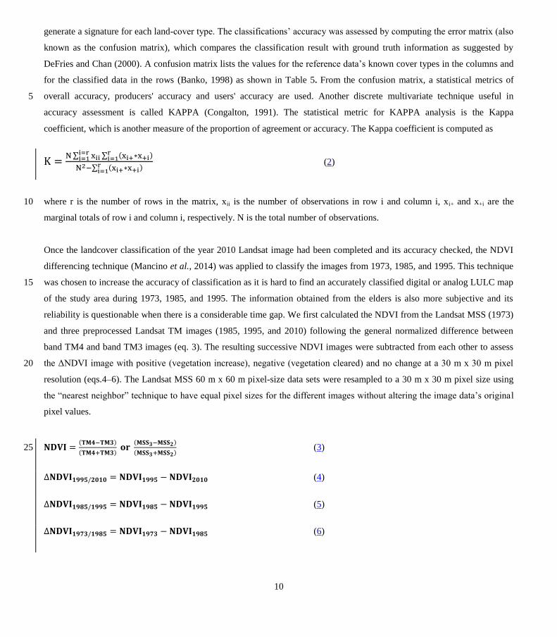
Once the landcover classification of the year 2010 Landsat image had been completed and its accuracy checked, the NDVI

differencing technique (Mancino et al., 2014) was applied to classify the images from 1973, 1985, and 1995. This technique

was chosen to increase the accuracy of classification as it is hard to find an accurately classified digital or analog LULC map 15

of the study area during 1973, 1985, and 1995. The information obtained from the elders is also more subjective and its

reliability is questionable when there is a considerable time gap. We first calculated the NDVI from the Landsat MSS (1973)

and three preprocessed Landsat TM images (1985, 1995, and 2010) following the general normalized difference between

band TM4 and band TM3 images (eq. 3). The resulting successive NDVI images were subtracted from each other to assess

the ΔNDVI image with positive (vegetation increase) negative (vegetation cleared) and no change at a 30 m x 30 m pixel 20

resolution (eqs.4–6). The Landsat MSS 60 m x 60 m pixel-size data sets were resampled to a 30 m x 30 m pixel size using

the “nearest neighbor” technique to have equal pixel sizes for the different images without altering the image data’s original

pixel values.

(3) 25

(4)

(5)

(6)

11

he ΔNDVI image was then reclassified using a threshold value calculated as μ ± n*σ; where μ represents the ΔNDVI pixels

value mean and σ the standard deviation. he threshold identifies three ranges in the normal distribution: (a) the left tail

(ΔNDVI < μ − n*σ) (b) the right tail (ΔNDVI > μ + n*σ) and (c) the central region of the normal distribution (μ − n*σ <

ΔNDVI < μ + n*σ). Pixels within the two tails of the distribution are characterized b significant landcover changes

whereas pixels in the central region represent no change. To be more conservative, n = 1 was selected for this study to 5

narrow the threshold ranges for reliable classification. he standard deviation (σ) is one of the most widel applied threshold

identification approaches for different natural environments based on different remotely sensed imagery (Hu et al., 2004;

Jensen, 1996; Lu et al., 2004; Mancino et al., 2014; Singh, 1989) as cited by Mancino et al. (2014).

ΔNDVI pixel values (2010–1995) in the central region of the normal distribution (μ − n*σ < ΔNDVI < μ + n*σ) represent an 10

absence of landcover change between two different periods (i.e., 1995 and 2010); therefore, pixels from 1995 corresponding

to no landcover change can be classified as similar to the 2010 landcover classes. Pixels with significant NDVI change are

reclassified using supervised classification, taking signatures from the already classified, no-change pixels. Likewise, 1985

and 1973 landcover images were classified based on the classified images of 1995 and 1985 respectively. Finally, after

classifying the raw Landsat images into different landcover classes, change detection, which requires the comparison of 15

independently produced classified images (Singb, 1989), was performed by the postclassification method. The

postclassification change-detection comparison was conducted to determine changes in LULC between two independently

classified maps from images of two different dates. Although this technique has some limitations, it is the most common

approach because it does not require data normalization between two dates (Singh, 1989). This is because data from two

dates are separately classified, thereby minimizing the problem of normalizing for atmospheric and sensor differences 20

between two dates.

4.3 SWAT hydrological model

The Soil and Water Assessment Tool (SWAT) is an open-source-code, semi-distributed model with a large and growing

number of model applications in a variety of studies ranging from catchment to continental scales (Allen et al., 1998; Arnold 25

et al., 2012; Neitsch et al., 2002). It enables the impact of LULC change and climate change on water resources to be

evaluated in a basin with varying soil, land use, and management practices over a set period of time (Arnold et al., 2012).

In SWAT, the watershed is divided into multiple sub-basins, which are further subdivided into hydrological response units

(HRUs) consisting of homogeneous landuse management, slope, and soil characteristics (Arnold et al., 1998; Arnold et al., 30

2012). HRUs are the smallest units of the watershed in which relevant hydrologic components such as evapotranspiration,

12

surface runoff and peak rate of runoff, groundwater flow, and sediment yield can be estimated. Water balance is the driving

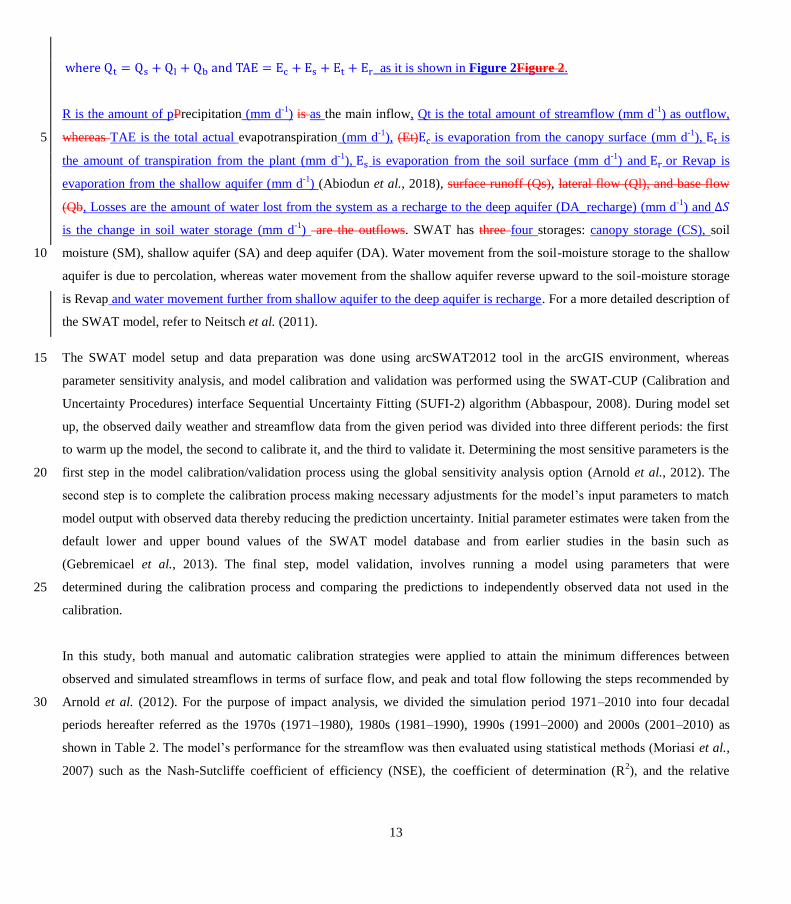
force behind all of the processes in the SWAT calculated using eq. 7,

(7)

5

where SWt is the final soil-water content (mm H2O), SWo is the initial soil-water content on day i (mm H2O), t is the time

(days), Rday is the amount of precipitation on day i (mm H2O), Qsurf is the amount of surface runoff on day i (mm H2O), Ql is

the amount of return flow on day i (mm H2O), Qb is the return flow from shallow aquifer on day i (mm H2O), Ea is the

amount of evapotranspiration from the canopy and soil surface on day i (mm H2O), Wseep Revap is the amount of water

transferred from the underlying shallow aquifer reverse upward to the soil-moisture storageentering the vadose zone from the 10

soil profile on day i (mm H2O) in response to water demand for evapotranspiration, and Ql DA_recharge is the amount of

return flow water recharge to deep aquifer on day i (mm H2O).

Runoff is calculated separately for each HRU and routed to obtain the total streamflow for the watershed using either the soil

conservation service (SCS) curve number (CN) method (Mockus, 1964) or Green & Ampt infiltration method (GAIM) 15

(Green and Ampt, 1911), see Figure 2Figure 2. However, spatial connectivity and interactions among HRUs are ignored.

Instead, the cumulative output of each spatially discontinuous HRU at the sub-watershed outlet is directly routed to the

channel (Pignotti et al., 2017). This lack of spatial connectivity among HRUs makes implementation and impact analysis of

spatially targeted management such as soil and water conservation structure difficult to incorporate into the model. Different

authors have made efforts to overcome this problem for instance, a grid-based version of the SWAT model (Rathjens et al., 20

2015) or landscape simulation on a regularized grid (Rathjens and Oppelt, 2012). Moreover, (Arnold et al., 2010) and

(Bosch et al., 2010) further modified SWAT so that it allows landscapes to be subdivided into catenas comprising upland,

hillslope, and floodplain units, and flow to be routed through these catenas. However, SWATgrid, developed to overcome

this limitation, remains largely untested and computationally demanding (Rathjens et al., 2015).

25

Hence, the standard SWAT CN method was chosen for this study because it was applied in many Ethiopian watersheds such

as (Gashaw et al., 2018; Gebremicael et al., 2013; Setegn et al., 2008; Woldesenbet et al., 2017b). Furthermore, its ability to

use daily input data (Arnold et al., 1998; Neitsch et al., 2011; Setegn et al., 2008) as compared to GAIM, which requires

subdaily precipitation as a model input, and that can be difficult to obtain in data-scare regions like the UBNRB. This study

focused on the effects of LULC changes and climate changes on the basin’s water balance components, which include the 30

components of inflows, outflows, evapotranspiration, losses and the change in storage as shown in the general water balance

eq. 8.

(8)

13

as it is shown in Figure 2Figure 2.

R is the amount of pPrecipitation (mm d-1

) is as the main inflow, Qt is the total amount of streamflow (mm d-1

) as outflow,

whereas TAE is the total actual evapotranspiration (mm d-1

), (Et) is evaporation from the canopy surface (mm d-1

), is 5

the amount of transpiration from the plant (mm d-1

), is evaporation from the soil surface (mm d-1

) and or Revap is

evaporation from the shallow aquifer (mm d-1

) (Abiodun et al., 2018), surface runoff (Qs), lateral flow (Ql), and base flow

(Qb, Losses are the amount of water lost from the system as a recharge to the deep aquifer (DA_recharge) (mm d-1

) and

is the change in soil water storage (mm d-1

) are the outflows. SWAT has three four storages: canopy storage (CS), soil

moisture (SM), shallow aquifer (SA) and deep aquifer (DA). Water movement from the soil-moisture storage to the shallow 10

aquifer is due to percolation, whereas water movement from the shallow aquifer reverse upward to the soil-moisture storage

is Revap and water movement further from shallow aquifer to the deep aquifer is recharge. For a more detailed description of

the SWAT model, refer to Neitsch et al. (2011).

The SWAT model setup and data preparation was done using arcSWAT2012 tool in the arcGIS environment, whereas 15

parameter sensitivity analysis, and model calibration and validation was performed using the SWAT-CUP (Calibration and

Uncertainty Procedures) interface Sequential Uncertainty Fitting (SUFI-2) algorithm (Abbaspour, 2008). During model set

up, the observed daily weather and streamflow data from the given period was divided into three different periods: the first

to warm up the model, the second to calibrate it, and the third to validate it. Determining the most sensitive parameters is the

first step in the model calibration/validation process using the global sensitivity analysis option (Arnold et al., 2012). The 20

second step is to complete the calibration process making necessar adjustments for the model’s input parameters to match

model output with observed data thereby reducing the prediction uncertainty. Initial parameter estimates were taken from the

default lower and upper bound values of the SWAT model database and from earlier studies in the basin such as

(Gebremicael et al., 2013). The final step, model validation, involves running a model using parameters that were

determined during the calibration process and comparing the predictions to independently observed data not used in the 25

calibration.

In this study, both manual and automatic calibration strategies were applied to attain the minimum differences between

observed and simulated streamflows in terms of surface flow, and peak and total flow following the steps recommended by

Arnold et al. (2012). For the purpose of impact analysis, we divided the simulation period 1971–2010 into four decadal 30

periods hereafter referred as the 1970s (1971–1980), 1980s (1981–1990), 1990s (1991–2000) and 2000s (2001–2010) as

shown in Table 2. he model’s performance for the streamflow was then evaluated using statistical methods ( oriasi et al.,

2007) such as the Nash-Sutcliffe coefficient of efficiency (NSE), the coefficient of determination (R2), and the relative

14

volume error (RVE %), which are shown by eq.89-1011. Furthermore, graphical comparisons of the simulated and observed

data as well as water balance checks were used to evaluate the model’s performance.

(9)

(10)

(11) 5

where Qm,i is the measured streamflow in m3s

-1, are the mean values of the measured streamflow (m

3s

-1), Qs,i is the

simulated streamflow in m3s

-1 , and are the mean values of simulated data in m

3s

-1.

4.4 SWAT simulations

Three different approaches were applied for assessing the effects of LULC change and climate change on streamflow and 10

water balance components. The first approach is to assess the response of streamflow for the combined effects of LULC

change and climate change. We followed the approach in (Marhaento et al., 2017) and divided the analysis period, 1971–

2010, into four periods of similar length (four decades). These are periods when land use changes are expected to change the

hydrological regime within a catchment (Marhaento et al., 2017; Yin et al., 2017a). The first period, the 1970s, was regarded

as the baseline period. The other periods, the 1980s, 1990s, and 2000s, were regarded as altered periods. LULC maps of 15

1973, 1985, 1995, and 2010 were used to represent LULC patterns during the 1970s, 1980s, 1990s, and 2000s respectively.

For analyses, the SWAT model was calibrated and validated for each respective period using the respective LULC map and

weather data (Table 2). The DEM and soil data sets remained unchanged. The differences between the simulation result of

the baseline and altered periods represent the combined effects of LULC and climate changes on streamflow and water

balance components 20

The second approach included simulations to attribute effects from LULC changes alone. It aimed to investigate whether

LULC change is the main driver for changes in water balance components. To identify the hydrological impacts caused

solely by LULC, "A fixing-changing" method was used (Marhaento et al., 2017; Woldesenbet et al., 2017b; Yan et al.,

2013; Yin et al., 2017b). The calibrated and validated SWAT model and its parameter settings in the baseline period were 25

forced by weather data from baseline period, 1973–1980, while changing only the LULC maps from 1985, 1995, and 2010,

keeping the DEM and soil data constant as suggested by (Hassaballah et al., 2017b; Marhaento et al., 2017; Woldesenbet et

al., 2017b; Yin et al., 2017b). We ran the calibrated SWAT model for the baseline period (1970s) four times changing only

the LULC map for the years 1973, 1985, 1995, and 2010 and retaining the constant weather data set from the 1970s (Table

15

2). The third approach is similar to the second, but the simulations are attributed only for climate changes. The calibrated

models for the base line period was run again four times, corresponding to the LULC periods using a unique LULC map of

the year 1973 but altering the four different periods of weather data sets for respective periods.

5. Results and discussions

5.1 Trend test 5

5.1.1 Rainfall

The summary of the MK trend tests result for the rainfall recorded at the 15 selected stations located in and around the

UBNRB revealed a mixed trends (increasing, decreasing, and no change). For daily time series, the computed probability

values (p-values) for seven stations was greater, although for eight stations it was less than the selected significance level (α

= 5 %). This means that no statistically significant trend existed in seven stations, but a monotonic trend occurred in the 10

remaining eight. Positive trends developed only at six stations, four of which were concentrated in the northern and central

highlands (Bahirdar, Dangila, Debre Markos, and G/bet). The other two stations, Assosa and Angergutten, are located in the

southwestern and southern lowlands (see Figure 1Figure 1). The other two stations, Alemketema and Nedjo, which are

located in the East and Southwest of the UBNRB, respectively showed a decreasing trend. On a monthly basis, the MK trend

test result showed that no trend existed in eleven stations while statistically non significant increasing trends exist in three 15

stations (Dangila, G/bet and Shambu) and a decreasing trend in Alemketema station. On an annual time scale, MK trend test

could not find any trend in eleven stations but did exhibit a trend in four stations. Debiremarkos, and Shambu stations

showed statistically non significant increasing trend while G/bet and Alemketema showed statistically significant positive

trend and non significant decreasing trend respectively. The trend analysis result for the annual rainfall time series agrees

well with a previous study by Gebremicael et al. (2013), who reported no significant annual rainfall change at eight out of 20

nine stations during the 1973–2005 period. Hence, it is interesting to note that the time scale of analysis is a critical factor in

determining the given trends.

The basin-wide areal UBNRB rainfall trend and change point analysis was again carried out on daily, monthly, seasonal, and

annual time scales using the MK and Pettitt tests respectively. We applied a widely used spatial interpolation technique, the 25

Thiessen polygon method, to calculate basin-wide rainfall series from station data. A summary is provided in Table 3 and

Figure 3. The MK test showed increasing trends for annual, monthly, and long-rainy-season rainfall series whereas no trend

for daily, short rainy and dry-season rainfall series appeared. The magnitude of trends for annual, monthly, and long-rainy-

season rainfall series are not statistically significant, as explained by the values of Sen's slope. However, the Pettitt test could

not detect any jump point in basin-wide rainfall series except for daily time-series rainfall (see Figure S01). 30

16

Previous studies such as (Conway, 2000; Gebremicael et al., 2013; Tesemma et al., 2010), conducted trend analysis of basin-

wide rainfall and reported that no significant change in annual and seasonal rainfall series across the UBNRB exists, which

contradicts with the result of this study. This disagreement could be due to the number of stations and their spatial

distribution across the basin, time period of the analysis, approach used to calculate basin-wide rainfall from gauging 5

stations, and data sources. Tesemma et al. (2010) used monthly rainfall data downloaded from Global Historical

Climatology Network (GHCN) data base and 10-day rainfall data for the 10 selected stations obtained from the National

Meteorological Service Agency of Ethiopia from 1963–2003. Conway (2000) also constructed basin-wide annual rainfall in

the UBNRB for the 1900–1998 period from the mean of 11 gauges. Furthermore, (Conway, 2000) employed simple linear

regressions over time to detect trends in annual rainfall series without removing the serial autocorrelation effects. 10

Gebremicael et al. (2013), used only nine stations from the 1970–2005 period. However, in this study, we used daily

observed rainfall data from 15 stations collected from Ethiopian Meteorological Agency from 1971–2010. The stations are

more or less evenly distributed over the UBNRB.

5.1.2 Streamflow

he K test’s result for dail monthl annual and seasonal (long and short rain season and dr season) streamflow time 15

series showed a positive trend, the magnitude of which is statistically significant, as summarized in Table 3 . The Pettitt test

also detected change point for daily, annual, and short-rainy-season streamflow but did not detect change point for monthly,

long, and dry season streamflow (see Figure 3 and Figure S02). The change point detected by the Pettitt test for annual

streamflow is in 1995 whereas for daily and short rainy seasons it is in 1985 and 1987, respectively. The result obtained from

the MK test agrees well with the findings in Gebremicael et al. (2013), who reported an increasing trend in the observed 20

annual short and long rain seasons’ streamflow at the l Diem gauging station but our results disagree to findings for dr -

season streamflow. Furthermore, the increasing trend of long-rainy-season streamflow agrees well with the result of

Tesemma et al. (2010), but disagrees with the results of short rainy season and annual flows. (Tesemma et al., 2010),

reported that the short rainy season and the annual flows are constant for the 1964–2003 period. This disagreement is likely

attributable to the difference in analysis period, as can be seen from Figure 3. The last seven years, 2004–2010, had 25

relatively higher streamflow records.

Although, the results of the MK test for annual and long-rainy-season rainfall and streamflow show an increasing trend for

the last 40 years in the UBNRB, the magnitude of Sen's slope for streamflow is much greater than it is for rainfall (Table 3).

Moreover, short-rainy-season streamflow shows a statistically significant positive increase whereas the rainfall shows no 30

change. The mismatch between rainfall and streamflow trend magnitude could be associated with evapotranspiration and

17

attributable to the combined effect of LULC change and climate change, infiltration rate due to changing soil properties,

rainfall intensity, and extreme events.

5.2 LULC change analysis

According to the confusion-matrix report overall accurac of 80 % producer’s accurac values for all classes ranged from

75.4 % to 100 %, user's accuracy values ranging from 83.7 % to 91.7 % and a kappa coefficient (k) of 0.77 were attained for 5

the 2010 classified image (Table 5). Monserud (1990) suggested a kappa value of <40 % as poor, 40–55 % fair, 55–70 %

good, 70–85 % very good, and >85 % as excellent. According to these ranges, the classification in this study has very good

agreement with the validation data set and meets the minimum accuracy requirements to be used for further change detection

and impact analysis.

10

The classified images of the basin (Figure 4) have shown different LULC proportions at four distinct time periods, as shown

in Figure 5. Cultivated land dominantly covers (62.9 %) of UBNRB, followed by bushes and shrubs (18 %), forest (17.4 %),

and water (1.74 %) in 1973. In 1985, cultivated land area increased to 65.6 %, followed by bushes and shrubs (18.3 %),

while forest decreased to 14.4 %, and water remained unchanged at 1.7 %. In 1995, cultivated land area further increased to

67.5 %, followed by bushes and shrubs (18.5 %). Forest further decreased to 12.2 % and water remained unchanged at 1.7 15

%. In 2010, cultivated land decreased to 63.9 %, bushes and shrubs increased to 18.8 %, forest increased to 15.6 %, and

water remained unchanged at 1.7 %. During the entire 1973–2010 period, cultivated land, along with bushes and shrubs

remained the major proportions compared to the other LULC classes. The highest increase (2.7 %) and the largest decrease

(−3.6 %) in cultivated land occurred during the 1973–1985 and 1995–2010 periods respectively. The largest increase in

bushes and shrubs was 0.3 % from 1973 to 1985, whereas the largest increase in forest coverage (3.4 %) was recorded during 20

the 1995–2010 period. Water coverage remained unchanged from 1973 to 2010.

Although, the image classification results show very good accuracy, uncertainties in classification could be expected. First,

as elsewhere in Ethiopia, LULC may change rapidly over the land surface of the basin and image reflectance may be

confusing due to the topography and variation in the image acquisition date. Landsat images were not all available for one 25

particular year or one season (as described under section 4.2.1); images from different years and different seasons might

harbor errors. Secondly, the workflow associated with LULC classification involves many steps and can be a source of

uncertainty. The errors are observed in the classified LULC map as shown in Figure 4. On the western side of the map in

Figure 4 (a) a rectangular section with forest appears, that completely disappears in 4(b). Rectangular forest cover appears in

the northern part of the country in 4(b), which again disappears completely in 4(c). In 4(d), forest cover with linear edges 30

(North-South) appears on the map’s eastern side. That being recognized, the land-cover mapping is reasonably accurate

overall, providing a good base for land-cover estimation and for providing basic information for the hydrological impact

analysis.

18

The rate of expansion of cultivated land before 1995 was higher than after 1995. Conversely, the area of the forest land

decreased in 1985 and 1995 with reference to the 1973 baseline. owever after 1995 the forest’s size increased again

whereas cultivated land decreased. The increased forest coverage and the decrease in cultivated land over the period 1995 to

2010 showed that the environment was recovering from the devastating drought, and forest clearing for firewood and 5

cultivation due to population growth has been minimized. This could be due to the afforestation program, which the

Ethiopian government initiated, and to the extensive soil and water conservation measures carried out by the community.

Since 1995, eucalyptus tree plantation expanded significantly across the country at homestead level for fire wood,

construction material, charcoal production, and income generation (Woldesenbet et al., 2017b). In summary, forest coverage

decreased by 1.8 %, while both bushes and shrubs as well as cultivated land increased by 0.8 % and 1 % respectively during 10

the 2010 period from the original 1973 level. This result agrees well with other studies (Gebremicael et al., 2013; Rientjes et

al., 2011; Teferi et al., 2013; Woldesenbet et al., 2017b), who reported a significant conversion of natural vegetation cover

into agricultural land.

5.3 SWAT model calibration and validation 15

he SWA model’s most sensitive parameters for simulating streamflow were identified using global sensitivit anal sis of

SWAT-CUP. Their optimized values were determined by the calibration process that Arnold et al. (2012) recommended.

Parameters such as SCS curve number (CN2), base flow alpha factor (ALPHA_BF), soil evaporation compensation factor

(ESCO), threshold water depth in the shallow aquifer required for return flow to occur ( WQ N) groundwater “revap”

coefficient (GW_REVAP), and available water capacity (SOL_AWC) were found to be the most sensitive parameters for the 20

streamflow predictions.

Figure 6 shows the calibration and the validation results for monthly streamflow hydrographs for each models. These results

revealed that the model represents the monthly hydrographs well as also indicated by R2, NSE, and RVE (%) statistical

performance measures (Table 6). For the calibration period, the values of R2, NSE, and RVE (%) range from 0.79 to 0.91, 25

0.74 to 0.91, and −3.4 % to 4 %, respectively. For the validation period they ranged from 0.84 to 0.94, 0.82 to 0.92 and −7.5

% to 7.2 % respectively. According to the rating of Moriasi et al. (2007) the SWA model’s performance over the UBNRB

can be categorized as very good, although underestimation was observed in the baseflow simulation. The optimal parameter

values of the four calibrated-model runs are shown in Table 7. A change was obtained for CN2 parameter values, which can

be attributed to the catchment’s response behavior. For instance, an increase in the absolute average (basin-wide) CN2 value 30

in the 1980s and 1990s from 72.9 to 74.7 and 75.6 compared to the 1970s respectively, indicate a reduction in forest

19

coverage and expansion of cultivated land. On the contrary, a decrease in CN2 value was attained during the period 1990s to

2000s from 75.6 to 73.6, attributed to the increase in forest coverage and reduction in cultivated land.

5.4 Combined effects of LULC change and climate change on streamflow and water balance components

The simulation results of the four independent, decadal-time-scale calibrated and validated SWAT model runs reflect the

combined effect of both LULC and climate change during the past 40 years (Table 8). From the simulation result, mean 5

annual streamflow increased by 16.9 % between the 1970s and the 2000s, while the observed mean annual streamflow

increased by 15.3 % for the same period. However, the rate of change is different in different decades. For example, it

increased by 3.4 % and 9.9 % during the 1980s and 1990s respectively from the baseline 1970s period.

The ratio of mean annual streamflow to mean annual precipitation (Qt/P) increased from 19.4 % to 22.1 % while the actual 10

evaporation to precipitation (Ea/P) ratio decreased from 61.1 % to 60.5 % from the 1970s to 2000s. Moreover, the ratio of

surface runoff to streamflow (Qs/Qt) increased notably from 40.7 % in the 1970s to 50.1 % and 55.4 % in the 1980s and

1990s respectively, and decreased to 43.7 % in the 2000s. In contrast, the base flow to streamflow ratio (Qb/Qt) notably

decreased from 17.1 % in the 1970s to 10.3 % and 3.2 % respectively during the 1980s and 1990s, but has increased to 20 %

in the 2000s. The result for surface runoff agrees to findings in (Gebremicael et al., 2013), but disagreement is observed for 15

baseflow. The study reported that surface runoff (Qs) contribution to the total river discharge increased by 75 %, while the

baseflow (Qb) decreased by 50 % from the 1970s to 2000s.

In general, 1.8 % forest cover loss and 1 % increased cultivated land combined with 2.2 % increased rainfall from the 1970s

to the 2000s led to a 16.9 % increase in simulated streamflow. The 1990s was the period during which the greatest 20

deforestation and expansion of cultivated land was reported; meanwhile, it is the time when the rainfall intensity and the

number of rainfall events have significantly increased compared to the 1970s and 1980s, as shown in Table 4Table 4. Hence,

the increased mean annual streamflow could be ascribed to the combined effects of LULC and climate change. In the case of

(Qs/Qt), the increasing pattern could be ascribed to increasing rainfall intensities and the expansion of cultivated land and

diminution of forest coverage, which might adversely affect soil/water storage and decrease rainfall infiltration, thereby 25

increasing water yield or streamflow. In contrast, the decreasing Qb/Qt is positively related to the increasing

evapotranspiration linked to both LULC and climate factors (Table 8). This hypothesis can be explained with the change in

CN2 parameter values obtained during calibration of the four SWAT model runs. The CN2 parameter value which is a

function of evapotranspiration derived from LULC, soil type, and slope increased in the 1980s and 1990s relative to the

1970s, and could be associated with the expansion of cultivated land and shrinkage of forest land. The increasing CN2 30

results reflect more surface runoff and less baseflow being generated.

20

Another important factor contributing to decreasing of surface runoff and increasing base flow ratio from 1990s to the 2000s

could be the establishment of soil and water conservation (SWC) measures. According to Haregeweyn et al. (2015), various

nationwide SWC initiatives such as Food for Work (FFW), Managing Environmental Resources to Enable Transition

(MERET) to more sustainable livelihoods, Productive Safety Net Programs (PSNP), Community Mobilization through free-

labor days, and the National Sustainable Land Management Project (SLMP) have been undertaken since the 1980s. 5

Haregeweyn et al. (2015) evaluated these initiatives’ effectiveness and concluded that communit labor mobilization seems

to be the best approach. This can reduce mean seasonal surface runoff by 40 %, with broad spatial variability ranging from 4

% in Andit Tid (northwest Ethiopia) to 62 % in Gununo (south Ethiopia).

5.5 Effects of an isolated LULC change on streamflow and water balance components

(Yan et al., 2013) used "A fixing -changing" method, which was also applied to this study, to identify the hydrological 10

impacts of LULC change alone. The calibrated and validated SWAT model and its parameter settings in the baseline period

was forced by weather data from the baseline 1973–1980 period while changing only the LULC maps from 1985, 1995, and

2010, keeping the DEM and soil data constant as suggested by Hassaballah et al. (2017a). The result from Figure 7Figure 7

indicated that Qs/Qt ratio changed from 40.7 % to 41.2 %, 41.9 %, and 40.9 % respectively by using the LULC maps from

1973, 1985, 1995 and 2010, whereas the Qb/Qt ratio changed from 17.1 % to 16.8 %, 16.5 %, and 16.9 % respectively. The 15

largest Qs/Qt ratio (41.9 %) and the smallest Qb/Qt ratio (16.5 %) were recorded with the 1995 LULC map. This could be

attributed to the 5.1 % reduction in forest coverage and 4.6 % increase in cultivated land with the 1995 LULC map relative

to the 1973 LULC map.

On a basin scale over a decadal time period, water gains mainly from precipitation. The losses are mainly due to runoff and 20

evapotranspiration (Oki et al., 2006) as the losses due to the deep percolation over the whole UBNRB is negligible

(Steenhuis et al., 2009). The long term mean annual deep percolation simulated in this study is about 16.7 mm constant in

four decadal periods, which is about 6 % of the total water yield. With the fixing-changing approach, the change in

streamflow attributable to LULC change was essentially the change in evapotranspiration between the two periods, as the

amount of precipitation was constant (1970s) and the change in water storage during the two periods was similar (Yan et al., 25

2013). Annual Ea losses from seasonal crops are smaller than those from forests, because seasonal crops transpire during a

relatively shorter time interval than perennial trees do (Yan et al., 2013). As a result, the actual mean annual Ea simulated by

the SWAT model was 871.6 mm at the baseline. It decreased to 871.4 mm and 871 mm in 1985 and 1995 respectively and

increased to 872.1 mm in 2010. This could be due to simultaneous expansion of cultivated land and shrinkage in forest

coverage in the 1985 and 1995 LULC maps relative to the 1973 base line. Furthermore, this deforestation may reduce 30

canopy interception of the rainfall, decrease soil infiltration by increasing raindrop impacts, and reducing plant transpiration,

which can significantly increase surface runoff and reducing base flow (Huang et al., 2013). Here, the evapotranspiration

change caused by the LULC change is minimal. As a result, the change for surface runoff and baseflow is not significant.

21

5.6 Effects of isolated climate change on streamflow and water balance components

The impacts of climate change are analyzed by running the four models using a unique LULC map from 1973 with its model

parameters while changing only the weather data sets from 1970s, 1980s, 1990s, and 2000s. The simulated water balance

components shown in Figure 7Figure 7 indicate that the Qs/Qt ratio increased from 40.7 % to 45.2 %, 45.6 %, and 46.2 %

during the 1970s, 1980s, 1990s and 2000s respectively, while the Qb/Qt ratio changed from 17.1 % to 13.5 %, 14.9 %, and 5

12.7 % for the same simulation periods. The decreasing Qb/Qt ratio for the altered periods compared to the baseline period

could be attributed to evapotranspiration changing from 872 mm to 854 mm, 906 mm, and 884 mm respectively in 1970s,

1980s, 1990s, and 2000s, which can be linked to temperature and amount of rainfall. However, it is important to know the

dominant rainfall-runoff process in the study area to fully understand the effect of climate change on the water balance

components. 10

Although, no detailed research has been conducted on the Upper Blue Nile basin to investigate the runoff-generation

processes, Liu et al. (2008) investigated the rainfall-runoff processes at three small watersheds located inside and around the

Upper Blue Nile basin, namely, Mayber, AnditTid, and Anjeni. Their analysis showed that, unlike in temperate watersheds,

in monsoonal climates, a given rainfall volume at the onset of the monsoon produces a different runoff volume than the same 15

rainfall at the end of the monsoon. Liu et al. (2008) and Steenhuis et al. (2009) showed that the ratio of discharge to

precipitation minus evapotranspiration, Q/(P − ET), increases with cumulative precipitation from the onset of monsoon. This

suggests that saturation excess processes play an important role in watershed response.

Furthermore, the infiltration rates that Engda (2009) measured in 2008 were compared with rainfall intensities in the Maybar 20

and Andit Tid watersheds located inside and around the UBNRB. In the Andit Tid watershed, which has an area of less than

500 ha, the measured infiltration rates at 10 locations were compared with rainfall intensities considered from the 1986 –

2004 period. The analysis showed that only 7.8 % of rainfall intensities were found to be higher than the lowest soil

infiltration rate of 25mm h-1

. Derib (2005) performed a similar analysis in the Maybar watershed (with a catchment area of

113 ha). The infiltration rates measured from 16 measurements ranged from 19 mm h-1

to 600 mm h-1

with a 240 mm h-1

25

average and 180 mm h-1

median whereas the average daily rainfall intensity from 1996 to 2004 was 8.5 mm hr-1

. Hence, he

suggested from these infiltration measurements that infiltration excess runoff is not a common feature in these watersheds.

From the above discussion points, it is to be noted that surface runoff could increase with increasing total rainfall amount

regardless of rainfall intensity. However, the mean annual rainfall amount in this study was decreasing from the 1970s to the 30

1980s (1428 mm and 1397 mm respectively) while the (Qs/Qt) ratio increased from 40.7 % to 45.2 %. Similarly, the mean

annual rainfall amount in the 1990s (1522 mm) was greater than the mean annual rainfall amount in the 2000s (1462 mm)

while the (Qs/Qt) increased from 45.6 % to 46.2 %. In contrast, climate indexes such as 99-percentile rainfall, SDII (ratio of

total precipitation amount to number of days when rainfall >1 mm (R1mm)), and number of days when rainfall >20 mm

22

(R20mm) increase consistently from 1970 to the 2000s, as shown in Table 4Table 4. This indicates that the increasing of

surface runoff might be due to an increasing of number of extreme rainfall events and rainfall intensity. Although, we did not

use hourly rainfall data for the SWAT model, this study suggested that infiltration excess of overland flow dominates the

rainfall-runoff processes in the UBNRB, not saturation excess of overland flow. The contradiction from the previous studies

might be due either to the limitation of the SWAT- CN method when applied in monsoonal climates or the overlooked of 5

tillage activities, which significantly impact the soil infiltration rate. Extensive tillage activities are carried out across the

basin at the beginning of the rainy season. Soils get disturbed as a result, which can increase the infiltration rate and

ultimately decrease the amount of rainfall converted to runoff.

Although the CN method is easy to use and provides acceptable results for discharge at the watershed outlet in many cases, 10

researchers have concerns about its use in watershed models (Steenhuis et al., 1995; White et al., 2011). The SWAT-CN

model relies with a statistical relationship between soil moisture condition and CN value obtained from plot data in the

United States with a temperate climate that was never tested in a monsoonal climate exhibiting two extreme soil moisture

conditions. In monsoonal climates, long periods of rain can lead to prolonged soil saturation whereas during the dry period,

the soil dries out completely, which may not happen in temperate climates (Steenhuis et al., 2009). Hence, further research 15

that considers bio-physical activities such as tillage and seasonal effects on soil moisture at representative watersheds of the

basin is necessary to properly assess the rainfall-runoff processes.

6. Conclusions

his stud ’s objectives were to understand the long-term variations of rainfall and streamflow in the UBNRB using

statistical techniques (MK and Pettitt tests), and to assess the combined and isolated effects of climate and LULC change 20

using a semi-distributed hydrological model (SWAT). Although the results of the MK test for annual and long-rainy-season

rainfall and streamflow show an increasing trend over the last 40 years, the magnitude of Sen's slope for streamflow is much

larger than the Sen's slope of areal rainfall. Moreover, for the short-rainy-season streamflow shows a statistically significant

positive increase while the rainfall shows no change. The mismatch of trend magnitude between rainfall and streamflow

could be attributed to the combined effect of LULC and climate change, associated with decreasing actual evapotranspiration 25

(Ea) and increasing rainfall intensity and extreme events.

LULC change detection was assessed by comparing the classified images. The result showed that the dominant process is

largely the expansion of cultivated land and decrease in forest coverage. The rate of deforestation is high during the 1973–

1995 period. This is probably due to the severe drought that occurred in the mid-1980s and to a large population increase 30

resulting from the expansion of agricultural land. On the other hand, forest coverage increased by 3.4 % during the period

1995 to 2010. This indicates that the environment was recovering from the devastating drought in the 1980s, regenerating of

23

forests as the result of afforestation program initiated by the Ethiopian government, and due to soil and water conservation

activities accomplished by the communities.

The SWAT model was used to analyze the combined and isolated effects of LULC and climate changes on the monthly

streamflow at the basin outlet (El Diem station, located on the Ethiopia-Sudan border). The result showed that the combined 5

effects of the LULC and climate changes increased the mean annual streamflow by 16.9 % from the 1970s to the 2000s. The

increased mean annual streamflow could be ascribed to the combined effects of LULC and climate change. The LULC

change alters the catchment responses. As a result, SWAT model parameter values could be changed. For instance, the

expansion of cultivation land and the shrinkage of forest coverage from 1973 to 1995 changed the basin average CN2

parameter values from 72.9 in 1973 to 74.7 and 75.6 in 1985 and 1995 respectively. Increasing of CN2 value might increase 10

surface runoff and decrease base flow. Similarly, the increase in rainfall intensity and extreme precipitation events led to a

substantial increase in Qs/Qt, a substantial decrease in Qb/Qt, and ultimately to increases in the streamflow during the 1971–

2010 simulation period.

The "fixing-changing" approach result using the SWAT model revealed that the isolated effect of LULC change could 15

potentially alter the streamflow generation processes. The result from Figure 7 shows that surface runoff is increasing while

baseflow is decreasing due to Expansion expansion of cultivated land and reduction of forest coverage that reduce

evapotranspiration during the periods 1985 and 1995 as compared to the baseline period 1973 LULC map. Furthermore, the

SWAT simulation result from Table 8 and Figure 7 revealed that the Revap is a significant contributor to the TAE in the

UBNRB for the last 40 years, with mean annual contribution ranged from 21.4–25.6 %, this could be due to the large 20

coverage of deep rooted Eucalyptus tree species that can access the saturated zone (Neitsch et al., 2011). The Revap

component in this study appears consistent with the results of (Abiodun et al., 2018; Benyon et al., 2006), who reported the

annual groundwater ET contribution to total ET ranged from 13–72 % and 20 % respectively for south-eastern Australia and

Sixth Creek Catchments. However, detail investigation for the contribution of depth to water table for Revap in the study

area is required which is beyond the scope of this study. might reduce evapotranspiration because seasonal crops transpire 25

less than perennial trees do (Yan et al., 2013) resulting in increased surface runoff. Alternatively, reduction of forest

coverage may reduce canopy interception of the rainfall, decrease the soil infiltration by increasing raindrop impacts, and

reduce plant transpiration, which can significantly increase surface runoff and reduce base flow (Huang et al., 2013). In

general, a 5.1 % reduction in forest coverage and a 4.6 % increase in cultivated land led to a 9.9 % increase in mean annual

streamflow from 1973 to 1995. This study provides a better understanding and substantial information about how climate 30

and LULC change affects streamflow and water balance components separately and jointly, which is useful for basin-wide

water resources management. The SWAT simulation indicated that the impacts of climate change are more substantial than

the impacts of LULC change, as shown in Figure 7. Surface water is no longer used for agriculture and plant consumption in

areas such as the UBNRB, where water-storage facilities are scarce. On the other hand, base flow provides the most reliable

24

source for the irrigation needed to increase agricultural production. Hence, the increasing amount of surface water and

diminished base flow caused by both LULC and climate changes negatively affect socio-economic developments in the

basin.

Protecting and conserving the natural forests and expanding soil-and-water conservation activities is therefore highly 5

recommended, not only to increase the base flow available for irrigation but also to reduce soil erosion. Doing so might

increase productivity, and improve the livelihoods and regional-water-resource-use cooperation. However, the uncertainties

of Landsat image classification and the model uncertainty of SWAT simulation might limit this study. To improve the

accuracy of LULC classification from Landsat images, further efforts such as integrating other images with Landsat images

through image-fusion techniques (Ghassemian, 2016) are required. The SWAT model does not adjust CN2 for slopes greater 10

than 5%. This could be significant in areas where the majority of the area has a slope greater than 5%, such as in the

UBNRB. We therefore suggest adjusting CN2 values for slope >5 % outside of the SWAT model might improve the results.

Moreover, further research involving rainfall intensity, infiltration rate, and event-based analysis of hydrographs and critical

evaluation of rainfall-runoff processes in the stud area might overcome this stud ’s limitations. inall the authors would

like to point out that the impacts of current and future water resource developments should be investigated to establish 15

comprehensive, holistic water resource management in the Nile basin.

Acknowledgements. The authors would like to thank the Ethiopian Ministry of Water, Irrigation and Electricity and the

Ethiopian National Meteorological Services Agency for providing the streamflow and meteorological data, respectively for

free. The authors would also like to express their gratitude to the anonymous referees and the editor, Prof. Axel Bronstert, 20

who gave constructive remarks and comments for enhancing the quality of the manuscript.

References

Abbaspour, C.K.: SWAT Calibrating and Uncertainty Programs. A User Manual. Eawag Zurich, Switzerland, 2008. 25

Abiodun, O.O., Guan, H., Post, V.E., Batelaan, O.: Comparison of MODIS and SWAT evapotranspiration over a complex terrain at different spatial scales. Hydrology and Earth System Sciences, 22(5), 2775-2794, 2018.

Alemseged, T.H., Tom, R.: Evaluation of regional climate model simulations of rainfall over the Upper Blue Nile basin. Atmospheric research, 161, 57-64, 2015. DOI:10.1016/j.atmosres.2015.03.013 30

Allen, R.G., Pereira, L.S., Raes, D., Smith, M.: Crop evapotranspiration-Guidelines for computing crop water requirements-FAO Irrigation and drainage paper 56. FAO, Rome, 300(9), D05109, 1998.

Arnold, J.G., Srinivasan, R., Muttiah, R.S., Williams, J.R.: Large area hydrologic modeling and assessment part I: Model development1. Wiley Online Library, 1998.

25

Arnold, J.G., Allen, P., Volk, M., Williams, J., Bosch, D.: Assessment of different representations of spatial variability on SWAT model performance. Transactions of the ASABE, 53(5), 1433-1443, 2010.

Arnold, J.G., Moriasi, D.N., Gassman, P.W., Abbaspour, K.C., White, M.J., Srinivasan, R., Santhi, C., Harmel, R., Van Griensven, A., Van Liew, M.W.: SWAT: Model use, calibration, and validation. Transactions of the ASABE, 55(4), 1491-1508, 2012. 5

Awulachew, S.B., McCartney, M., Steenhuis, T.S., Ahmed, A.A.: A review of hydrology, sediment and water resource use in the Blue Nile Basin, 131. IWMI, 2009.

Banko, G.: A review of assessing the accuracy of classifications of remotely sensed data and of methods including remote sensing data in forest inventory IASA Interim Report. IIASA, Laxenburg, Austria, IR-98-08, 1998. 10

BCEOM: Abbay river basin integrated development master plan project, phase 3 main report. Ministry of Water Resources, Addis Ababa, Ethiopia, Volume I, Main report, 1998.

Benyon, R.G., Theiveyanathan, S., Doody, T.M.: Impacts of tree plantations on groundwater in south-eastern Australia. Australian Journal of Botany, 54(2), 181-192, 2006.

Bewket, W., Sterk, G.: Dynamics in land cover and its effect on stream flow in the Chemoga watershed, Blue Nile 15

basin, Ethiopia. Hydrological Processes, 19(2), 445-458, 2005. Bosch, D., Arnold, J., Volk, M., Allen, P.: Simulation of a low-gradient coastal plain watershed using the SWAT

landscape model. Transactions of the ASABE, 53(5), 1445-1456, 2010. Cheung, W.H., Senay, G.B., Singh, A.: Trends and spatial distribution of annual and seasonal rainfall in Ethiopia.

International Journal of Climatology, 28(13), 1723-1734, 2008. 20

Congalton, R.G.: A review of assessing the accuracy of classifications of remotely sensed data. Remote sensing of environment, 37(1), 35-46, 1991.

Conway, D.: The climate and hydrology of the Upper Blue Nile River. The Geographical Journal, 166(1), 49-62, 2000.

DeFries, R., Chan, J.C.-W.: Multiple criteria for evaluating machine learning algorithms for land cover 25

classification from satellite data. Remote Sensing of Environment, 74(3), 503-515, 2000. Derib, S.D.: Rainfall-runoff processes at a hill-slope watershed: case of simple models evaluation at Kori-Sheleko

Catchments of Wollo, Ethiopia, M. Sc. Thesis, 2005. Engda, T.A.: Modeling rainfall, runoff and soil loss relationships in the northeastern highlands of Ethiopia, andit

tid watershed, Citeseer, 2009. 30

Gashaw, T., Tulu, T., Argaw, M., Worqlul, A.W.: Modeling the hydrological impacts of land use/land cover changes in the Andassa watershed, Blue Nile Basin, Ethiopia. Science of The Total Environment, 619, 1394-1408, 2018.

Gebremicael, T., Mohamed, Y., Betrie, G., van der Zaag, P., Teferi, E.: Trend analysis of runoff and sediment fluxes in the Upper Blue Nile basin: A combined analysis of statistical tests, physically-based models and 35

landuse maps. Journal of Hydrology, 482, 57-68, 2013. Ghassemian, H.: A review of remote sensing image fusion methods. Information Fusion, 32, 75-89, 2016. Green, W.H., Ampt, G.: Studies on Soil Phyics. The Journal of Agricultural Science, 4(01), 1-24, 1911. Haile, A.T., Akawka, A.L., Berhanu, B., Rientjes, T.: Changes in water availability in the Upper Blue Nile basin

under the representative concentration pathways scenario. Hydrological sciences journal, 62(13), 2139-40

2149, 2017. DOI:10.1080/02626667.2017.1365149 Hamed, K.H., Rao, A.R.: A modified Mann-Kendall trend test for autocorrelated data. Journal of Hydrology,

204(1-4), 182-196, 1998.

26

Haregeweyn, N., Tsunekawa, A., Nyssen, J., Poesen, J., Tsubo, M., Tsegaye Meshesha, D., Schütt, B., Adgo, E., Tegegne, F.: Soil erosion and conservation in Ethiopia: a review. Progress in Physical Geography, 39(6), 750-774, 2015.

Hassaballah, K., Mohamed, Y., Uhlenbrook, S., Biro, K.: Analysis of streamflow response to land use and land cover changes using satellite data and hydrological modelling: case study of Dinder and Rahad 5

tributaries of the Blue Nile (Ethiopia–Sudan). Hydrology and Earth System Sciences, 21(10), 5217, 2017a.

Hassaballah, K., Mohamed, Y., Uhlenbrook, S., Biro, K.: Analysis of streamflow response to land use land cover changes using satellite data and hydrological modelling: case study of Dinder and Rahad tributaries of the Blue Nile (Ethiopia/Sudan). 2017b. 10

Hayes, D.J., Sader, S.A.: Comparison of change-detection techniques for monitoring tropical forest clearing and vegetation regrowth in a time series. Photogrammetric engineering and remote sensing, 67(9), 1067-1075, 2001.

Hu, Y., De Jong, S., Sluiter, R.: A modeling-based threshold approach to derive change/no change information over vegetation area, Proceedings of the “12 International Conference on Geoinformatics-Geospatial 15

Information Research: Bridging the Pacific and Atlantic”. University of Gävle (Sweden), pp. 647-654, 2004.

Huang, J., Wu, P., Zhao, X.: Effects of rainfall intensity, underlying surface and slope gradient on soil infiltration under simulated rainfall experiments. Catena, 104, 93-102, 2013.

Jensen, J.R.: Introductory digital image processing: a remote sensing perspective. Prentice-Hall Inc., 1996. 20

Kendall, M.: Rank correlation methods. 1975. Liu, B.M., Collick, A.S., Zeleke, G., Adgo, E., Easton, Z.M., Steenhuis, T.S.: Rainfall‐discharge relationships for a

monsoonal climate in the Ethiopian highlands. Hydrological Processes, 22(7), 1059-1067, 2008. Lu, D., Mausel, P., Batistella, M., Moran, E.: Comparison of land-cover classification methods in the Brazilian

Amazon Basin. Photogrammetric engineering & remote sensing, 70(6), 723-731, 2004. 25

Mancino, G., Nolè, A., Ripullone, F., Ferrara, A.: Landsat TM imagery and NDVI differencing to detect vegetation change: assessing natural forest expansion in Basilicata, southern Italy. iForest-Biogeosciences and Forestry, 7(2), 75, 2014.

Mann, H.B.: Nonparametric Tests Against Trend. Econometrica, 13(3), 245-259, 1945. Marhaento, H., Booij, M.J., Rientjes, T., Hoekstra, A.Y.: Attribution of changes in the water balance of a tropical 30

catchment to land use change using the SWAT model. Hydrological Processes, 31(11), 2029-2040, 2017. McCartney, M., Alemayehu, T., Easton, Z.M., Awulachew, S.B.: Simulating current and future water resources

development in the Blue Nile River Basin. The Nile River Basin: water, agriculture, governance and livelihoods. Routledge-Earthscan, Abingdon, 269-291, 2012.

Mekonnen, D.F., Disse, M.: Analyzing the future climate change of Upper Blue Nile River basin using statistical 35

downscaling techniques. Hydrology and Earth System Sciences, 22(4), 2391-2408, 2018. Melesse, A., Abtew, W., Dessalegne, T., Wang, X.: Low and high flow analyses and wavelet application for

characterization of the Blue Nile River system. Hydrological processes, 24(3), 241, 2009. Mengistu, D., Bewket, W., Lal, R.: Recent spatiotemporal temperature and rainfall variability and trends over

the Upper Blue Nile River Basin, Ethiopia. International Journal of Climatology, 34(7), 2278-2292, 2014. 40

Mockus, V.: National engineering handbook,Section 4:Hydrology, 630, 1964. Monserud, R.A.: Methods for comparing global vegetation maps. 1990.

27

Moriasi, D.N., Arnold, J.G., Van Liew, M.W., Bingner, R.L., Harmel, R.D., Veith, T.L.: Model evaluation guidelines for systematic quantification of accuracy in watershed simulations. Trans. Asabe, 50(3), 885-900, 2007.

Neitsch, S., Arnold, J., Kiniry, J.e.a., Srinivasan, R., Williams, J.: Soil and water assessment tool user’s manual version 2000. GSWRL report, 202(02-06), 2002.

Neitsch, S.L., Arnold, J.G., Kiniry, J.R., Williams, J.R.: Soil and water assessment tool theoretical documentation 5

version 2009, Texas Water Resources Institute, 2011. NMA: Annual climate buletien for the year 2013. National Meteorological Agency, Meteorological Data and

Climatology Directorate, Addis Ababa, Ethiopia, http://www.ethiomet.gov.et/bulletins/bulletin_viewer/bulletins/348/2013_Annual_Bulletin/en, 2013.

Oki, T., Kanae, S.: Global hydrological cycles and world water resources. science, 313(5790), 1068-1072, 2006. 10

Pettitt, A.: A non-parametric approach to the change-point problem. Applied statistics, 126-135, 1979. Pignotti, G., Rathjens, H., Cibin, R., Chaubey, I., Crawford, M.: Comparative Analysis of HRU and Grid-Based

SWAT Models. Water, 9(4), 272, 2017. Polanco, E.I., Fleifle, A., Ludwig, R., Disse, M.: Improving SWAT model performance in the upper Blue Nile Basin

using meteorological data integration and subcatchment discretization. Hydrology and Earth System 15

Sciences, 21(9), 4907, 2017. Rathjens, H., Oppelt, N.: SWATgrid: An interface for setting up SWAT in a grid-based discretization scheme.

Computers & geosciences, 45, 161-167, 2012. Rathjens, H., Oppelt, N., Bosch, D., Arnold, J.G., Volk, M.: Development of a grid‐based version of the SWAT

landscape model. Hydrological processes, 29(6), 900-914, 2015. 20

Rientjes, T., Haile, A., Kebede, E., Mannaerts, C., Habib, E., Steenhuis, T.: Changes in land cover, rainfall and stream flow in Upper Gilgel Abbay catchment, Blue Nile basin-Ethiopia. Hydrology and Earth System Sciences, 15(6), 1979, 2011.

Seleshi, Y., Zanke, U.: Recent changes in rainfall and rainy days in Ethiopia. International journal of climatology, 24(8), 973-983, 2004. 25

Sen, P.K.: Estimates of the regression coefficient based on Kendall's tau. Journal of the American statistical association, 63(324), 1379-1389, 1968.

Setegn, S.G., Srinivasan, R., Dargahi, B.: Hydrological modelling in the Lake Tana Basin, Ethiopia using SWAT model. The Open Hydrology Journal, 2(1), 2008.

Singb, A.: Digital change detection techniques using remotelyWsensed data. International Journal of Remote 30

Sensing, 10(6), 989L1003, 1989. Singh, A.: Review article digital change detection techniques using remotely-sensed data. International journal

of remote sensing, 10(6), 989-1003, 1989. Steenhuis, T.S., Winchell, M., Rossing, J., Zollweg, J.A., Walter, M.F.: SCS runoff equation revisited for variable-

source runoff areas. Journal of Irrigation and Drainage Engineering, 121(3), 234-238, 1995. 35

Steenhuis, T.S., Collick, A.S., Easton, Z.M., Leggesse, E.S., Bayabil, H.K., White, E.D., Awulachew, S.B., Adgo, E., Ahmed, A.A.: Predicting discharge and sediment for the Abay (Blue Nile) with a simple model. Hydrological processes, 23(26), 3728-3737, 2009.

Teferi, E., Bewket, W., Uhlenbrook, S., Wenninger, J.: Understanding recent land use and land cover dynamics in the source region of the Upper Blue Nile, Ethiopia: Spatially explicit statistical modeling of systematic 40

transitions. Agriculture, ecosystems & environment, 165, 98-117, 2013.

28

Tekleab, S., Mohamed, Y., Uhlenbrook, S., Wenninger, J.: Hydrologic responses to land cover change: the case of Jedeb mesoscale catchment, Abay/Upper Blue Nile basin, Ethiopia. Hydrological Processes, 28(20), 5149-5161, 2014.

Tesemma, Z.K., Mohamed, Y.A., Steenhuis, T.S.: Trends in rainfall and runoff in the Blue Nile Basin: 1964–2003. Hydrological processes, 24(25), 3747-3758, 2010. 5

Uhlenbrook, S., Mohamed, Y., Gragne, A.: Analyzing catchment behavior through catchment modeling in the Gilgel Abay, upper Blue Nile River basin, Ethiopia. Hydrology and Earth System Sciences, 14(10), 2153-2165, 2010.

USBR: Land and water resources of the Blue Nile basin, Ethiopia. Main report. United States Bureau of Reclamation, Washington, DC., 1964. 10

Von Storch, H.: Misuses of Statistical Analysis in Climate Research, Analysis of Climate Variability. Springer, pp. 11-26, 1995.

White, E.D., Easton, Z.M., Fuka, D.R., Collick, A.S., Adgo, E., McCartney, M., Awulachew, S.B., Selassie, Y.G., Steenhuis, T.S.: Development and application of a physically based landscape water balance in the SWAT model. Hydrological Processes, 25(6), 915-925, 2011. 15

Woldesenbet, T.A., Elagib, N.A., Ribbe, L., Heinrich, J.: Gap filling and homogenization of climatological datasets in the headwater region of the Upper Blue Nile Basin, Ethiopia. International Journal of Climatology, 37(4), 2122-2140, 2017a.

Woldesenbet, T.A., Elagib, N.A., Ribbe, L., Heinrich, J.: Hydrological responses to land use/cover changes in the source region of the Upper Blue Nile Basin, Ethiopia. Science of the Total Environment, 575, 724-741, 20

2017b. Yan, B., Fang, N., Zhang, P., Shi, Z.: Impacts of land use change on watershed streamflow and sediment yield: an

assessment using hydrologic modelling and partial least squares regression. Journal of Hydrology, 484, 26-37, 2013.

Yin, J., He, F., Xiong, Y.J., Qiu, G.Y.: Effects of land use/land cover and climate changes on surface runoff in a 25

semi-humid and semi-arid transition zone in northwest China. Hydrology and Earth System Sciences, 21(1), 183, 2017a.

Yin, J., He, F., Xiong, Y.J., Qiu, G.Y.: Effects of land use/land cover and climate changes on surface runoff in a semi-humid and semi-arid transition zone in northwest China. Hydrology and Earth System Sciences, 21(1), 183-196, 2017b. 30

Yue, S., Pilon, P., Phinney, B., Cavadias, G.: The influence of autocorrelation on the ability to detect trend in hydrological series. Hydrological Processes, 16(9), 1807-1829, 2002.

Yue, S., Wang, C.: The Mann-Kendall test modified by effective sample size to detect trend in serially correlated hydrological series. Water Resources Management, 18(3), 201-218, 2004.

35

40

29

Table 1: he UBNRB’s areal long term (1971–2010) mean annual and seasonal rainfall and streamflow

Amount Contribution (%)

Station Kiremit Belg Bega Total Kiremit Belg Bega Mean Area (km2)

Flow (m3s

-1) 3506.3 300.4 1018.4 4825.1 72.7 6.2 21.1 1608 172254

Flow (BCM) 36.4 3.1 10.6 50.7

Rainfall (mm) 1070.1 140.8 238.9 1449.8 73.8 9.7 16.5

Kiremit: long rainy season, Belg: short rainy season, Bega: dry season

Table 2: Data sets of the baseline and altered periods for the SWAT simulation used to analyze the combined and isolated

effect of LULC and climate changes on streamflow and water balance components 5

Model run

no. Combined effect

Isolated LULC change

effect

Isolated climate change

effect

Remark

Climate data

set

LULC

map

Climate data

set

LULC

map

Climate data

set

LULC

map

1 1970s 1973 1970s 1973 1970s 1973 Base period

2 1980s 1985 1970s 1985 1980s 1973

altered

Period1

3 1990s 1995 1970s 1995 1990s 1973

altered

Period2

4 2000s 2010 1970s 2010 2000s 1973

altered

Period3

Table 3: K and Pettitt tests for the UBNRB’s rainfall and streamflow after PW at different time scales

Stream flow Rainfall

p-value p-value

Time

scale After* Before*

Sen's

slope:

Change

point Pettit test After* Before*

Sen's

slope

Change

point Pettit test

Daily < 0.0001 < 0.0001 0.013 1987 Increasing 0.387 0.953 0.000 1988 Increasing

Monthly < 0.0001 0.031 0.378

No change 0.010 0.640 0.009

No change

annually < 0.0001 0.009 9.619 1995 Increasing 0.006 0.260 1.886

No change

Kiremit < 0.0001 0.014 20.30

No change 0.010 0.348 1.364

No change

Belg < 0.0001 0.004 3.593 1985 Increasing 0.822 0.935 0.068

No change

Bega 0.000 0.214 4.832

No change 0.527 0.755 0.169

No change

* Before and after TFPW; p: probability at 5% significance level

10

30

Table 4: Summar of the UBNRB’s precipitation indices at decadal time series

Indices 1970s 1980s 1990s 2000s

Mean (mm) 4.17 4.05 4.42 4.16

95 percentile (mm) 12.57 12.52 13.66 13.31

99 percentile (mm) 17.34 17.77 19.44 19.65

1-day max (mm) 27.15 25.67 32.24 32.38

R20mm (days) 16 15 30 35

SDII (mm/day) 7.22 7.38 7.66 7.77

SDII is the ratio of total precipitation (mm) to R1mm (days).

Table 5: Confusion (error) matrix for the 2010 land use/cover classification map

LULC class Water Forest Cultivated

Bushes

and

shrubs Row total

Producers’

accuracy

Water 44 0 0 0 44 100

Forest 1 46 6 8 61 75.4

Cultivated land 2 3 77 15 97 79.4

Bushes and shrubs 1 3 9 73 86 84.9

Column total 48 52 92 86 288

User's accuracy (%) 91.7 88.5 83.7 84.9

Over all accuracy(%) 80

Kappa 0.77

5

Table 6: he SWA model’s statistical performance measure values

Period R2 NSE RVE (%)

1970s

Calibration (1973–1977) 0.79 0.74 −3.41

Validation (1978–1980) 0.84 0.83 7.18

1980s

Calibration (1983–1987) 0.80 0.74 −0.72

Validation (1988–1990) 0.86 0.82 0.73

1990s

Calibration (1993–1997) 0.91 0.91 1.79

Validation (1998–2000) 0.87 0.84 −3.56

2000s

Calibration (2003–2007) 0.86 0.86 3.99

Validation (2008–2010) 0.94 0.92 −7.51

10

31

Table 7: SWAT sensitive model parameters and their (final) calibrated values for the four model runs

Parameter

Optimum value

1970s 1980s 1990s 2000s

R-CN2 0.88 0.91 0.92 0.9

a-Alpha-BF 0.028 0.028 0.028 0.028

V-GW_REVAPMN 0.7 0.45 0.7 0.34

V-GWQMN 750 750 750 750

V-REVAPMN 550 450 425 550

a-ESCO −0.85 −0.85 −0.85 −0.85

R-SOL_AWC 6.5 6.5 6.5 6.5

R: value from the SWAT database is multiplied by a given value; V: replace the initial parameter by the given value;

a: adding the given value to initial parameter value. 5

Table 8: Mean annual water-balance-components analysis in the Upper Blue Nile River Basin (mm/year) by considering

LULC and climate change over respective periods. All streamflow estimates are for El Diem station.

Unit 1970s 1980s 1990s 2000s

Precipitation (P) mm 1428.1 1397.1 1522.2 1462.5

Surface flow (Qs) mm 112.8 143.4 168.6 141.4

Lateral flow (Ql) mm 116.8 113.4 125.9 117.6

Base flow (Qb) mm 47.3 29.6 9.8 64.7

Total water yield (Qt) mm 276.9 286.3 304.3 323.7

Revap (from shallow aquifer) mm 269.2 257.2 310.6 241.0

PET mm 1615.1 1627.3 1614.7 1732.9

Ea (Ec+Et+Es) mm 871.6 852.6 904.3 885.0

TAE mm 1140.8 1109.8 1214.9 1126.0

Recharge (to deep aquifer) mm 16.7 15.0 16.7 16.3

Total water yield (Qt) mm 276.9 286.3 304.3 323.7

Change in soil water content mm -6.3 -14.0 -13.7 -3.5

Qs/Qt % 40.7 50.1 55.4 43.7

Qb/Qt % 17.1 10.3 3.2 20.0

Qt/P % 19.4 20.5 20.0 22.1

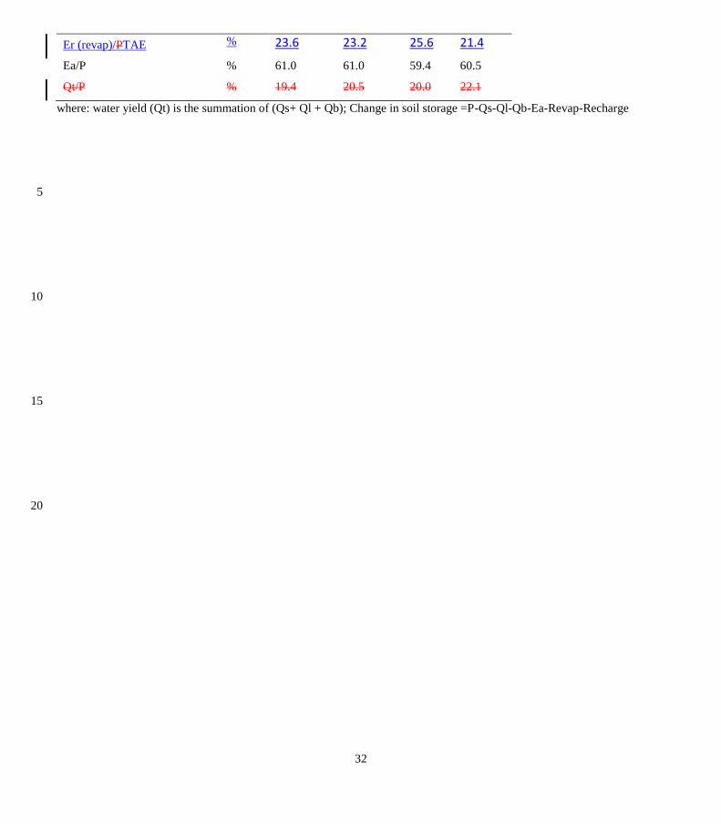
32

Er (revap)/PTAE % 23.6 23.2 25.6 21.4

Ea/P % 61.0 61.0 59.4 60.5

Qt/P % 19.4 20.5 20.0 22.1

where: water yield (Qt) is the summation of (Qs+ Ql + Qb); Change in soil storage =P-Qs-Ql-Qb-Ea-Revap-Recharge

5

10

15

20

33

Figure 1: Locations of study area and meteorological and discharge stations, with the Digital Elevation Model (DEM) data as the

background (where: 1: Stations used for SWAT model, 2: Stations used for trend analysis, 3: Stations removed from the analysis).

5

HRUn

Sub-catchmentt

Catchment outlett

Routing

HRU1

P

Ec+Et

DA

SM

SA

CS

DA_recharge

Er=

Rev

ap

Perc

Qs

Ql

Qb

Qt

Es

TAE

34

Figure 2: Schematic representation of the SWAT model structure modified from (Marhaento et al., 2017). P is precipitation; CS is canopy

storage; TAE is total actual evapotranspiration; Ec is evaopration from the canopy surface; Es is evaporation from the soil surface; Et is

transpiration from plants; perc is percolation from the soil storage to shallow aquifer; SM is soil moisture storage; SA is shallow aquifer;

Er=Revap is evaporation from the shallow aquifer; Qt is total streamflow; DA is deep aquifer; HRU is hydrological response unit; Qb is 5 base flow; Ql is lateral flow; Qs is surface runoff

1200

1300

1400

1500

1600

1700

1,970 1,980 1,990 2,000 2,010 2,020

Prec

ipita

tion

(mm

)

Year

Areal rainfall

mu = 1450

1000

1200

1400

1600

1800

2000

2200

2400

1,970 1,980 1,990 2,000 2,010 2,020

Stre

amfl

ow (m

3 s-1)

Year

Streamflow

mu1 = 1510 mu2 = 1784

y = 1.8344x + 1412.2R² = 0.0403

1,200

1,300

1,400

1,500

1,600

1,700

1,800

1971 1976 1981 1986 1991 1996 2001 2006

Rain

fall

(m

m)

Year

Areal rainfall

y = 10.474x + 1399.1R² = 0.2226

800

1,000

1,200

1,400

1,600

1,800

2,000

2,200

2,400

1971 1976 1981 1986 1991 1996 2001 2006

Str

eam

flo

w(m

3s-

1)

Year

Streamflow

a) b)

c) d)

35

Figure 3: The Pettitt homogeneity test a) annual rainfall, b) annual flow of the UBNRB, c) linear trend of mean annual

rainfall and d) linear trend of mean annual streamflow.

5

Figure 4: Landcover map of UBNRB derived from Landsat images a) 1973, b) 1985, c) 1995, and d) 2010

10

a) b)

a) b)

d) c)

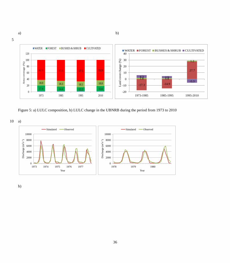
36

a) b)

5

Figure 5: a) LULC composition, b) LULC change in the UBNRB during the period from 1973 to 2010

a) 10

b)

17.4 14.4 12.2 15.6

18.0 18.3 18.5 18.8

62.9 65.6 67.5 63.9

0

20

40

60

80

100

120

1973 1985 1995 2010

Are

a c

overa

ge (

%)

WATER FOREST BUSHES & SHRUB CULTIVATED

-17.3 -14.9

27.7

1.8 1.4

1.2

4.3 2.9

-5.3

-20

-10

0

10

20

30

40

1973-1985 1985-1995 1995-2010

Lan

d c

over

chan

ge

(%)

WATER FOREST BUSHES & SHRUB CULTIVATED

0

2000

4000

6000

8000

10000

1973 1974 1975 1976 1977

Dis

ch

arg

e (

m3s-1

)

Year

Simulated Observed

0

2000

4000

6000

8000

10000

1978 1979 1980

Dis

ch

arg

e (

m3s-1

)

Year

Simulated Observed

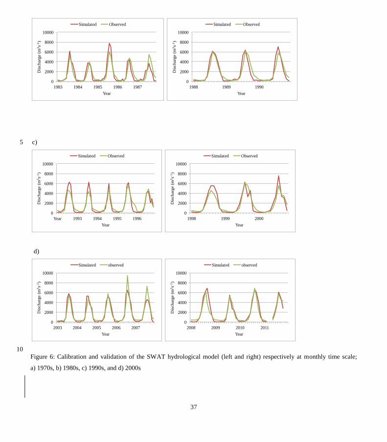
37

c) 5

d)

10

Figure 6: Calibration and validation of the SWAT hydrological model (left and right) respectively at monthly time scale;

a) 1970s, b) 1980s, c) 1990s, and d) 2000s

0

2000

4000

6000

8000

10000

1983 1984 1985 1986 1987

Dis

ch

arg

e (

m3s-1

)

Year

Simulated Observed

0

2000

4000

6000

8000

10000

1988 1989 1990

Dis

ch

arg

e (

m3s-1

)

Year

Simulated Observed

0

2000

4000

6000

8000

10000

Year 1993 1994 1995 1996

Dis

ch

arg

e (

m3s-1

)

Year

Simulated Observed

0

2000

4000

6000

8000

10000

1998 1999 2000

Dis

ch

arg

e (

m3s-1

)

Year

Simulated Observed

0

2000

4000

6000

8000

10000

2003 2004 2005 2006 2007

Dis

ch

arg

e (

m3s-1

)

Year

Simulated observed

0

2000

4000

6000

8000

10000

2008 2009 2010 2011

Dis

ch

arg

e (

m3s-1

)

Year

Simulated observed

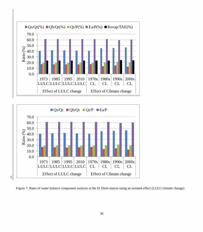
38

5

Figure 7: Ratio of water balance component analysis at the El Diem station using an isolated effect (LULC/climate change)

0.0

10.0

20.0

30.0

40.0

50.0

60.0

70.0

1973 LULC

1985 LULC

1995 LULC

2010 LULC

1970s CL

1980s CL

1990s CL

2000s CL

Effect of LULC change Effect of Climate change

Rat

io (

%)

Qs/Qt(%) Qb/Qt(%) Qt/P(%) Ea/P(%) Revap/TAE(%)

0.0

10.0

20.0

30.0

40.0

50.0

60.0

70.0

1973 LULC

1985 LULC

1995 LULC

2010 LULC

1970s CL

1980s CL

1990s CL

2000s CL

Effect of LULC change Effect of Climate change

Rat

io (

%)

Qs/Qt Qb/Qt Qt/P Ea/P