dealing with data quality in smart home environments
TRANSCRIPT
Journal of
Actuator NetworksSensor and
Article
Dealing with Data Quality in Smart HomeEnvironments—Lessons Learned from a SmartGrid PilotAlessandro Leonardi 1,*, Holger Ziekow 2, Martin Strohbach 1 and Panayotis Kikiras 1
1 AGT International, Hilpertstraße 35 64295 Darmstadt, Germany; [email protected] (M.S.);[email protected] (P.K.)
2 Furtwangen University, Robert-Gerwig-Platz 1 78120 Furtwangen, Germany; [email protected]* Correspondence: [email protected]; Tel.: +49-6151-460-5195
Academic Editor: Ioannis ChatzigiannakisReceived: 8 December 2015; Accepted: 14 February 2016; Published: 3 March 2016
Abstract: Over the last years, we have witnessed increasing interconnection between the physical anddigital world. The so called Internet of Things (IoT) is becoming more and more a reality in applicationdomains like manufacturing, mobile computing, transportation, and many others. However, despitepromising huge potential, the application domain of smart homes is still at its infancy and lags behindother fields of IoT. A deeper understanding of this type of techno-human system is required to makethis vision a reality. In this paper, we report findings from a three year pilot that sheds light on thechallenges of leveraging IoT technology in the home environment. In particular, we provide detailson data quality issues in real-world deployments. That is, we analyze application level data forerrors in measurements as well as issues in the end-to-end communication. Understanding whatdata errors to expect is crucial for understanding the smart building domain and paramount forbuilding successful applications. With our work, we provide insights in a domain of IoT that hastremendous growth potential and help researchers as well as practitioners to better account for thedata characteristics of smart homes.
Keywords: data quality; internet of things; smart home
1. Introduction
The internet of things is promising to revolutionize almost all aspects of our life. From the waythat we experience and communicate with our environment to the way that we manufacture ourproducts and conduct business. This revolution is heavily based on the deployment of a myriadof smart things that sense, act, and communicate with the users and among themselves in order toprovide advanced services. One of the first areas that are starting to experience this revolution is“smart homes”. According to a definition by the United Kingdom Department of Trade and Industry“A smart home is a dwelling incorporating a communications network that connects the key electrical appliancesand services, and allows them to be remotely controlled, monitored or accessed.” An interpretation of thiscould be that a smart home is a house that includes multiple sense and actuate systems that allowsto the users fully control and monitor functions such as lightning, heating and cooling, security andaccess, etc. From the aforementioned definition of the common smart home scenarios, it is clear thata smart home has rigid networking requirements for the connectivity of the smart things with theactuators and with the operators of the system; which are in the near zero latency range (e.g., if youneed to open a garage door or a valve in a heating system the acceptable latency for the user is at thesub-second range). We have faced similar strict requirements during our deployment for the datacollection and processing. This time the main issue was not the latency but the quality of the data.The quality of the data is affecting the results of the analytics and therefore it is fundamental for the
J. Sens. Actuator Netw. 2016, 5, 5; doi:10.3390/jsan5010005 www.mdpi.com/journal/jsan

J. Sens. Actuator Netw. 2016, 5, 5 2 of 24
precision of the system to deal with all root causes during collection, transfer, processing, and analysisof the data beforehand.
The remainder of the paper is structured as follows. Section 2 provides an overview of thePeerEnergyCloud project and discusses the overall system architecture. Section 3 describes the dataquality challenges that we faced during the deployment with focus on the main analytical componentsof our system. Section 4 presents the detailed analysis of the data quality issues we faced when pilotingthe system together with technical details of the key components in our test bed and the mechanismsfor addressing the encountered challenges. Section 5 discuss similar projects and, finally, we concludethe paper and discuss future work in Section 6.
2. Project Background
In this paper, we present analysis of data that we acquired throughout a three year pilot withsmart home technology. The pilot was conducted as part of the PeerEnergyCloud project [1], whichfunded by the German federal ministry of technology. We describe the project background and thesetting for our data collection in this section.
The PeerEnergyCloud was conducted between 2011 and of 2014 by a consortium of academicinstitutions and industry. The goal was to coordinate energy consumption within local neighborhoodsto better utilize locally available renewable energy. Specifically, it aimed at finding a means to influenceconsumption behavior, so that energy from privately owned solar panels is consumed within theimmediate neighborhood. Such an adaption of consumption behavior is of high interest for electricalgrid operators, because it improves grid stability and saves investments in grid infrastructure [2].In addition, the project explored ways of how grid operators can provide additional services tothe home owners on top of the piloted infrastructure. The PeerEnergyCloud project addressed thedevelopment of analytics technologies that enable a smarter use of energy. Specific use cases aredetailed in Section 3. All scenarios are driven by a deeper understanding of energy consumption onthe level of individual households. The pilot in PeerEnergyCloud enabled this work though a cloudbased infrastructure for data collection, processing, and service provisioning.
A central aspect of the project was the piloting of smart home sensor systems and applications.The smart home systems are the backbone of the PeerEnergyCloud project approach. Smart homesolutions are the enabling technology that allows home owners to better understand and managetheir energy consumption. As such, the technology provides the entry point for applications thathelp to optimize the consumption behavior and to deliver additional services. The pilot in thePeerEnergyCloud project allows deep insights into the operations of smart home system under realworld conditions. Throughout the project, we collected data from smart home systems over a period ofup to three years. This enables a long term analysis of the properties of smart home data and providesthe basis for the results in this paper.
2.1. System Architecture
As depicted in Figure 1, our system consists of two parts: the operational infrastructure thatcollects data from households and an analytics infrastructure that we used for analyzing the collecteddata. Data is transferred into the analytics infrastructure via batch process that export the data fromPostgreSQL into Hadoop Distributed File System (HDFS) as Comma Separated Values (CSV) files.We used Impala to convert the CSV data to the parquet file format.

J. Sens. Actuator Netw. 2016, 5, 5 3 of 24
J. Sens. Actuator Netw. 2016, 5, 5 3 of 23
contain a relay to switch on/off the devices remotely and consume only a few mA for all the operations carried out.
• Multi-sensors able to acquire various ambient parameters like brightness, temperature, humidity, motion detection. Also in this case, measured data are sent via wireless connection (ZigBee) to the Home Gateway.
• Home Gateway which collects all measured data, stores them in a local cache and sends them using a secure connection to a remote Backend. The gateway provides at least two interfaces: one wireless interface (ZigBee) able to connect to the smart plugs; one Ethernet/Wi-Fi interface to the home modem/router to have Internet access. The analytics infrastructure consists of a small four-node Cloudera cluster. For the quality analysis
presented in this paper we were only using the Impala service using YARN as a resource manager.
Figure 1. System Overview.
The smart metering ecosystem may facilitate a multitude of applications and value added services (VAS). Security and privacy are a major concern in this context as these applications and services directly affect users' everyday life and may collect a substantial amount of sensitive data. In order to enable these services new security and privacy solutions are required. The user needs simple-to-use mechanisms that provide a transparent view on all data that is collected and processed within such an ecosystem. The user should be in perfect control of which data is collected, how it is processed and which data is exchanged with which third parties. The PEC Privacy Dashboard is one of the components developed for the PEC project designed to define and control access to sensors. The user interacts with this component dashboard to review current access control rules and to modify as well as add rules (see Figure 2).
Figure 2. User interface for controlling privacy settings.
Figure 1. System Overview.
PostgreSQL was chosen because it provided an easy way of storing and querying the data usingthe SQL query language. However, we experienced that PostgreSQL is insufficient for performingad hoc queries as needed for the results presented in this paper. Running Impala on top of HDFSfilled this gap. We also used additional infrastructures such as Hadoop’s Map Reduce, Storm, and thecomplex event processing engine Esper [3].
The technological components of the system (of interest for this work) are the following:
‚ Smart plugs with remote control, containing a high-precision energy meter to measure parameterslike voltage, current, frequency, power, and electrical consumption (KWh). Measured data aresent via wireless connection (ZigBee [4]) to the Home Gateway. Smart plugs contain a relay toswitch on/off the devices remotely and consume only a few mA for all the operations carried out.
‚ Multi-sensors able to acquire various ambient parameters like brightness, temperature, humidity,motion detection. Also in this case, measured data are sent via wireless connection (ZigBee) to theHome Gateway.
‚ Home Gateway which collects all measured data, stores them in a local cache and sends themusing a secure connection to a remote Backend. The gateway provides at least two interfaces: onewireless interface (ZigBee) able to connect to the smart plugs; one Ethernet/Wi-Fi interface to thehome modem/router to have Internet access.
The analytics infrastructure consists of a small four-node Cloudera cluster. For the quality analysispresented in this paper we were only using the Impala service using YARN as a resource manager.
The smart metering ecosystem may facilitate a multitude of applications and value added services(VAS). Security and privacy are a major concern in this context as these applications and servicesdirectly affect users’ everyday life and may collect a substantial amount of sensitive data. In order toenable these services new security and privacy solutions are required. The user needs simple-to-usemechanisms that provide a transparent view on all data that is collected and processed within suchan ecosystem. The user should be in perfect control of which data is collected, how it is processedand which data is exchanged with which third parties. The PEC Privacy Dashboard is one of thecomponents developed for the PEC project designed to define and control access to sensors. The userinteracts with this component dashboard to review current access control rules and to modify as wellas add rules (see Figure 2).
The user input from the privacy dashboard is transformed into statements in a given policylanguage. In order to make our approach as open as possible, XACML is used as the policy decisionlanguage, as its expressiveness allows full coverage of all necessary aspects for our applicationscenarios. These policy statements are then used to evaluate access requests from various applications.More details can be found in [5].

J. Sens. Actuator Netw. 2016, 5, 5 4 of 24
J. Sens. Actuator Netw. 2016, 5, 5 3 of 23
contain a relay to switch on/off the devices remotely and consume only a few mA for all the operations carried out.
• Multi-sensors able to acquire various ambient parameters like brightness, temperature, humidity, motion detection. Also in this case, measured data are sent via wireless connection (ZigBee) to the Home Gateway.
• Home Gateway which collects all measured data, stores them in a local cache and sends them using a secure connection to a remote Backend. The gateway provides at least two interfaces: one wireless interface (ZigBee) able to connect to the smart plugs; one Ethernet/Wi-Fi interface to the home modem/router to have Internet access. The analytics infrastructure consists of a small four-node Cloudera cluster. For the quality analysis
presented in this paper we were only using the Impala service using YARN as a resource manager.
Figure 1. System Overview.
The smart metering ecosystem may facilitate a multitude of applications and value added services (VAS). Security and privacy are a major concern in this context as these applications and services directly affect users' everyday life and may collect a substantial amount of sensitive data. In order to enable these services new security and privacy solutions are required. The user needs simple-to-use mechanisms that provide a transparent view on all data that is collected and processed within such an ecosystem. The user should be in perfect control of which data is collected, how it is processed and which data is exchanged with which third parties. The PEC Privacy Dashboard is one of the components developed for the PEC project designed to define and control access to sensors. The user interacts with this component dashboard to review current access control rules and to modify as well as add rules (see Figure 2).
Figure 2. User interface for controlling privacy settings. Figure 2. User interface for controlling privacy settings.
2.2. Sensor Deployment
We provided some volunteers with smart home packages that have been installed on theirpremises. A package consisted of a set of sensors and a gateway to enable communication with acloud infrastructure. In addition, volunteers had access to some cloud-based smart home applications.The volunteers conducted the installations on their own account and they were free in choosing howand where to install the sensors. Some of the initial installations were done under supervision frommembers of the research team and some completely unsupervised. From this point on, we continuouslycollected the data without any supervision of the deployment, in some cases for more than three years.
During the installation we faced some connectivity issues related to the connection of ZigBeedevices to the gateway. The ZigBee connectivity heavily depended on the conditions within thevarious households. That is, the material of the wall and the distance between sensors (i.e., number ofstories) had a strong impact on the connection quality. We managed to support deployment in largehouseholds by leveraging the multi-hop capabilities of the ZigBee protocol and by carefully selectingdeployment positions (i.e., plugs in stairways between stories).
3. Data Quality Challenges in Smart Home Applications
Data quality is an important factor in any data driven application but the particular requirementsvary between the particularities of the targeted use cases. Smart home technology is an enabler fora broad range of applications for a variety of stakeholders. The PeerEnergyCloud covered use casesthat address the utilization of smart home technology for private users within the home as well as foroptimizing the operations of utilities. The different applications are sensitive to different data qualityaspects and to varying degrees. This section discusses the impact of data quality along sample usecases from the PeerEnergyCloud project. In particular, we address the data quality aspects of (a) dataaccuracy; (b) completeness; and (c) delay. Here, data accuracy refers to the correctness of capturedsensor measurements. Completeness refers to the presence of absence of gaps in the sensor stream, anddelay refers to the time gap between a change in the physical world and the reflection of this change inthe software system. We discuss the significance of each aspect along the sample applications belowand provide corresponding technical analysis throughout the paper. Specifically, we discuss (1) areal-time dashboard; (2) long-term consumption analysis; and (3) short-term consumption prediction.

J. Sens. Actuator Netw. 2016, 5, 5 5 of 24
3.1. Real-Time Dashboard
Trial participants of the PeerEnergyCloud project were provided with a set of web-basedapplications to analyze their consumption data. One of the key applications in this set is a real-timedashboard. Real-time in this application means, that users should get an instant feedback aboutchanging their consumption. This is, when the user switches a device, the observed values mustchange quick enough for the user to relate the consumption change to his or her switching action.Figure 3 shows a screenshot of the application. The dashboard provides live statistics of device specificenergy consumption. Available visualizations are the current values as number as well as line chartsthat get continuously updated. The application furthermore enabled switching of devices via theweb-interface.
J. Sens. Actuator Netw. 2016, 5, 5 5 of 23
lead to negative perceptions. Note that this aspect does not only relate to the correctness of sensor measurements. The completeness and timeliness of arrival is even more important. When users switch a device on, they expect the displayed load curves to go up immediately. However, missing or delayed values may cause a misalignment between the expected and the displayed data. Incorrect reflection of loads in the real-time dashboard is very prominently perceived by the users (e.g., I just switched the lamp is on but shows still a flat consumption line at zero). This makes dealing with gaps and delays in the data particularly challenging for such types of applications.
Figure 3. Real-time dashboard.
3.2. Long-Term Consumption Analysis
Part of the application portfolio within the PeerEnergyCloud project were applications that provide a long term analysis of device specific energy consumption. That is, consumption is displayed aggregated over days, week or month. Figures 4 and 5 show sample screenshots of such applications from the pilot. The aggregated long term analysis was a key feature for many pilot participants. This is because it allows a better understanding how much a particular devices contribute to the overall consumption and how energy efficient they are overall. For instance, several users were keen to monitor the consumption of their washing machine to understand the impact of using older machines compared to modern and more energy efficient solutions.
Data quality for long term analysis must be sufficient to yield reasonably accurate results. Compared to real-time analysis, it is less critical if some measurements as missing, as long as the long term aggregate is not significantly impacted. Also, the applications do not display real-time updates and hence users do not directly perceive small gaps in the data stream. Thus, delays in measurements play a minor role for this type of application. However, throughout the pilot we encountered data quality issues that got to the users attention with negative effects on the perceived usefulness and trust in the system. The relevant data quality aspects are related to data accuracy and completeness. Erroneous measurements can in extreme cases lead to considerable distortion of the aggregate values and noticeably implausible results. Also, long gaps can cause apparent deviations from the actual and displayed consumption. For instance, a user may remember to have briefly watched TV yesterday but—in case of a longer measurement gap—may see zero consumption for the TV on that day. Thus, while being less time critical, scrutinizing data for display is required and the quality of the input streams has a significant impact on the applications.
Figure 3. Real-time dashboard.
Throughout the PeerEnergyCloud project this application was one of the main ways how usersinteracted with the system. Displaying correct data is vital for the perceived usefulness and the trustin the technical solution. In particular, values that are implausible can easily be spotted by users andlead to negative perceptions. Note that this aspect does not only relate to the correctness of sensormeasurements. The completeness and timeliness of arrival is even more important. When users switcha device on, they expect the displayed load curves to go up immediately. However, missing or delayedvalues may cause a misalignment between the expected and the displayed data. Incorrect reflection ofloads in the real-time dashboard is very prominently perceived by the users (e.g., I just switched thelamp is on but shows still a flat consumption line at zero). This makes dealing with gaps and delays inthe data particularly challenging for such types of applications.
3.2. Long-Term Consumption Analysis
Part of the application portfolio within the PeerEnergyCloud project were applications thatprovide a long term analysis of device specific energy consumption. That is, consumption is displayedaggregated over days, week or month. Figures 4 and 5 show sample screenshots of such applicationsfrom the pilot. The aggregated long term analysis was a key feature for many pilot participants. This isbecause it allows a better understanding how much a particular devices contribute to the overallconsumption and how energy efficient they are overall. For instance, several users were keen tomonitor the consumption of their washing machine to understand the impact of using older machinescompared to modern and more energy efficient solutions.

J. Sens. Actuator Netw. 2016, 5, 5 6 of 24J. Sens. Actuator Netw. 2016, 5, 5 6 of 23
Figure 4. Pilot application showing tabular overview the consumption history.
Figure 5. Pilot application showing the consumption over time ranges.
3.3. Short-Term Consumption Prediction
A key challenge for grid operators is balancing out production and consumption at any time. Growing numbers of solar panels on private homes in Germany introduce additional complexity to this challenge. For efficiency reasons, it is desirable to balance out the production and consumption locally in the grid and avoid long distance energy transmission. One goal of the PeerEnergyCloud project was to investigate means for improving local balancing by proactively influencing energy consumption in households. Proactive steering however, requires household specific prediction of the consumption at least a few minutes ahead [6].
Figure 4. Pilot application showing tabular overview the consumption history.
J. Sens. Actuator Netw. 2016, 5, 5 6 of 23
Figure 4. Pilot application showing tabular overview the consumption history.
Figure 5. Pilot application showing the consumption over time ranges.
3.3. Short-Term Consumption Prediction
A key challenge for grid operators is balancing out production and consumption at any time. Growing numbers of solar panels on private homes in Germany introduce additional complexity to this challenge. For efficiency reasons, it is desirable to balance out the production and consumption locally in the grid and avoid long distance energy transmission. One goal of the PeerEnergyCloud project was to investigate means for improving local balancing by proactively influencing energy consumption in households. Proactive steering however, requires household specific prediction of the consumption at least a few minutes ahead [6].
Figure 5. Pilot application showing the consumption over time ranges.
Data quality for long term analysis must be sufficient to yield reasonably accurate results.Compared to real-time analysis, it is less critical if some measurements as missing, as long as the longterm aggregate is not significantly impacted. Also, the applications do not display real-time updatesand hence users do not directly perceive small gaps in the data stream. Thus, delays in measurementsplay a minor role for this type of application. However, throughout the pilot we encountered dataquality issues that got to the users attention with negative effects on the perceived usefulness andtrust in the system. The relevant data quality aspects are related to data accuracy and completeness.Erroneous measurements can in extreme cases lead to considerable distortion of the aggregate valuesand noticeably implausible results. Also, long gaps can cause apparent deviations from the actual and

J. Sens. Actuator Netw. 2016, 5, 5 7 of 24
displayed consumption. For instance, a user may remember to have briefly watched TV yesterdaybut—in case of a longer measurement gap—may see zero consumption for the TV on that day. Thus,while being less time critical, scrutinizing data for display is required and the quality of the inputstreams has a significant impact on the applications.
3.3. Short-Term Consumption Prediction
A key challenge for grid operators is balancing out production and consumption at any time.Growing numbers of solar panels on private homes in Germany introduce additional complexity tothis challenge. For efficiency reasons, it is desirable to balance out the production and consumptionlocally in the grid and avoid long distance energy transmission. One goal of the PeerEnergyCloudproject was to investigate means for improving local balancing by proactively influencing energyconsumption in households. Proactive steering however, requires household specific prediction of theconsumption at least a few minutes ahead [6].
Throughout the project, we investigated prediction mechanisms that apply household specificprediction models on the real-time streams of consumption data. Our experiments show that highresolution and device specific measurements enable improvements in the short-term predictionaccuracy. Yet, data quality issues can impact the prediction. One aspect is that faulty input datacauses prediction errors. Another aspect, is that missing data reduces the prediction accuracy as well.We have shown in experiments, that high temporal resolutions in measurements can positively impactthe prediction accuracy [5]. Thus, the data accuracy is major concern for short-term consumptionprediction. The aspect of delay however is comparatively less relevant. This is because the temporalscope for predictions is in the order of at least several minutes. Thus, compared in dashboards forreal-time consumption monitoring, delays of a few seconds have less impact on an application level.
4. Analysis of Data Quality
This section presents the results of our analysis of data quality. We first provide an overviewof the overall characteristics of the captured data and the observed anomalies. Subsequently,we report on findings regarding the arrival rates of sensors messages and the downtimes ofinfrastructure components.
4.1. Overview of Data Characteristics
Overall, the data quality of six households has been analyzed. Each household contained six orseven smart plugs and all but one contained three or four multi-sensor devices.
Table 1 details the distribution of sensing devices and the total number of measurements. Whilemost households provided between 520 and 650 Mio measurements, Houses 4 and 6 only delivereda fraction of the measurements. This is due to the fact that House 6 was configured with a lowersampling rate and only reported one sample per minute as compared to a sample of every two secondsat the other houses. Each smart plug includes six sensors and each multi-sensor device contains fivesensors. Tables 1 and 2 give an overview of the captured data types and total number of measurements.
Table 1. Overview of sensing devices.
HOUSE Smart Plugs Multisensors Sensor Devices Measurements
House 1 6 3 9 522,269,428House 2 7 4 11 636,928,123House 3 7 4 11 534,912,560House 4 7 3 10 159,202,670House 5 7 4 11 648,517,430House 6 7 0 7 18,822,263
Total 41 18 59 2,520,652,474

J. Sens. Actuator Netw. 2016, 5, 5 8 of 24
Table 2. Overview of sensors.
Measurement Type Deployed Device Unit Data Type
Power Smart Plug Watt FloatFrequency Smart Plug Hertz FloatOn state Smart Plug n/a ON|OFFVoltage Smart Plug Volt FloatCurrent Smart Plug Ampere Float
Work Smart Plug kWh FloatMotion Multi Sensor Motion intensity index Float
Battery State Multi Sensor n/a LOW|OKBrightness Multi Sensor Lumen Float
Battery Voltage Multi Sensor Volt FloatTemperature Multi Sensor Degree Celsius Float
Overall, we examined the data quality of over 2.5 billion measurements that were stored in a single,de-normalized, partitioned Impala table backed by parquet files using the default snappy compression.Several additional, auxiliary tables were created supporting the analysis. The files were stored onHDFS using our default replication factor of three. The net storage, i.e., not counting the replicatedblocks, of the compressed parquet files amounts to approximately 17 GB of data. As comparison theuncompressed net storage of the same data on HDFS amounts to approximately 287 GB. Figure 6shows the aggregated number of measurements per month for each household.
J. Sens. Actuator Netw. 2016, 5, 5 8 of 23
Overall, we examined the data quality of over 2.5 billion measurements that were stored in a single, de-normalized, partitioned Impala table backed by parquet files using the default snappy compression. Several additional, auxiliary tables were created supporting the analysis. The files were stored on HDFS using our default replication factor of three. The net storage, i.e., not counting the replicated blocks, of the compressed parquet files amounts to approximately 17 GB of data. As comparison the uncompressed net storage of the same data on HDFS amounts to approximately 287 GB. Figure 6 shows the aggregated number of measurements per month for each household.
Figure 6. Aggregated number of measurements per month for each household.
In the following subsections, we first describe conversion errors of number and non-number types and then describe the data characteristics for each measurement type. Those measurement types that did not reveal any insights are not mentioned. For instance, we did not find any irregularities in the brightness readings.
4.1.1. Conversion Errors
All the measurements were initially stored as strings. As a first step towards assessing the data quality we validated the data types. Except for the on state of the smart plug and the battery state of the multi-sensor, values should represent floating point values. However 452 values could not be cast to a floating point. This affected all corresponding measurement types of the smart plug. None of the multi-sensors were affected by such parsing errors. In addition, there exists a single record of a current measurement where the actual measurement is completely missing (empty string). Of the non-floating point measurement types there were only two erroneous values of measurement type “on state”. The values were ONMS = 239 and ON6 and are likely caused by formatting errors in the sensor message or errors in the parsing process.
4.1.2. Work Anomalies
Ideally, work values would increase monotonically over time as the measurement was intended to represent the accumulated work since deploying the sensor. However, house occupants could reset the plug which would lead to reporting 0 kWh followed by monotonically increasing values. An event in which a preceding value was truly larger than the current value we therefore considered as anomaly. The overall number of anomalies is insignificant: out of the 421,589,929 work values only 17,876 anomalies were observed in our dataset. However we realized that only an insignificant part of the anomalies could have resulted from resetting the smart plug. The majority, i.e. between 98.19% and 99.99% of the anomalies per household showed as a non-zero drop in the work value. Our assumption is that this is due to network latencies that lead to messages arriving at the gateway out of order.
Figure 6. Aggregated number of measurements per month for each household.
In the following subsections, we first describe conversion errors of number and non-number typesand then describe the data characteristics for each measurement type. Those measurement types thatdid not reveal any insights are not mentioned. For instance, we did not find any irregularities in thebrightness readings.
4.1.1. Conversion Errors
All the measurements were initially stored as strings. As a first step towards assessing the dataquality we validated the data types. Except for the on state of the smart plug and the battery state ofthe multi-sensor, values should represent floating point values. However 452 values could not be castto a floating point. This affected all corresponding measurement types of the smart plug. None ofthe multi-sensors were affected by such parsing errors. In addition, there exists a single record of acurrent measurement where the actual measurement is completely missing (empty string). Of thenon-floating point measurement types there were only two erroneous values of measurement type“on state”. The values were ONMS = 239 and ON6 and are likely caused by formatting errors in thesensor message or errors in the parsing process.
J. Sens. Actuator Netw. 2016, 5, 5 9 of 24
4.1.2. Work Anomalies
Ideally, work values would increase monotonically over time as the measurement was intendedto represent the accumulated work since deploying the sensor. However, house occupants could resetthe plug which would lead to reporting 0 kWh followed by monotonically increasing values. Anevent in which a preceding value was truly larger than the current value we therefore considered asanomaly. The overall number of anomalies is insignificant: out of the 421,589,929 work values only17,876 anomalies were observed in our dataset. However we realized that only an insignificant part ofthe anomalies could have resulted from resetting the smart plug. The majority, i.e. between 98.19% and99.99% of the anomalies per household showed as a non-zero drop in the work value. Our assumptionis that this is due to network latencies that lead to messages arriving at the gateway out of order.
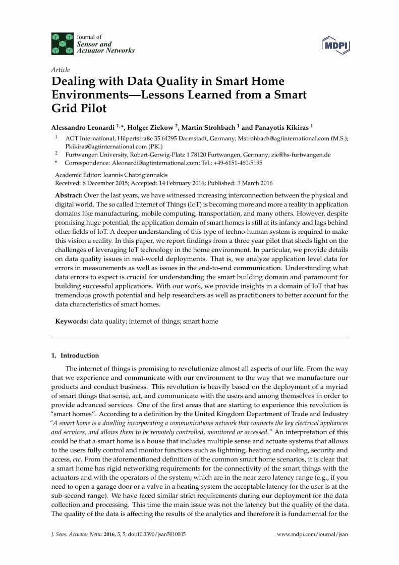
4.1.3. Voltage Anomalies
Figure 7 shows that most of the voltage values vary between 227 and 239 V and most values arearound the average. We also looked at the minimum and maximum voltage values for each sensor inorder to check whether they deliver plausible values. In terms of the maximum values (not shown inthe figure) only two sensors exhibited unusual high values. One sensor reported a maximum voltageof over 1392 V whereas the second sensor reported 2099 V. Both sensors were deployed in House 3.
J. Sens. Actuator Netw. 2016, 5, 5 9 of 23
4.1.3. Voltage Anomalies
Figure 7 shows that most of the voltage values vary between 227 and 239 V and most values are around the average. We also looked at the minimum and maximum voltage values for each sensor in order to check whether they deliver plausible values. In terms of the maximum values (not shown in the figure) only two sensors exhibited unusual high values. One sensor reported a maximum voltage of over 1392 V whereas the second sensor reported 2099 V. Both sensors were deployed in House 3.
Figure 7. Scatter plot showing basic descriptive statistics for voltage measurements by sensor. Lower bound and upper bound represent the +/- one standard deviation.
4.1.4. Current
When considering the minimum current measurements, it can be seen from Figure 8 that for a majority of sensors, i.e., 33 sensors, the minimum value equals zero. One sensor in House 6 reported an extremely high minimum value of 173.
Figure 8. Minimum current measurements per sensor.
Figure 7. Scatter plot showing basic descriptive statistics for voltage measurements by sensor. Lowerbound and upper bound represent the +/- one standard deviation.
4.1.4. Current
When considering the minimum current measurements, it can be seen from Figure 8 that for amajority of sensors, i.e., 33 sensors, the minimum value equals zero. One sensor in House 6 reportedan extremely high minimum value of 173.

J. Sens. Actuator Netw. 2016, 5, 5 10 of 24
J. Sens. Actuator Netw. 2016, 5, 5 9 of 23
4.1.3. Voltage Anomalies
Figure 7 shows that most of the voltage values vary between 227 and 239 V and most values are around the average. We also looked at the minimum and maximum voltage values for each sensor in order to check whether they deliver plausible values. In terms of the maximum values (not shown in the figure) only two sensors exhibited unusual high values. One sensor reported a maximum voltage of over 1392 V whereas the second sensor reported 2099 V. Both sensors were deployed in House 3.
Figure 7. Scatter plot showing basic descriptive statistics for voltage measurements by sensor. Lower bound and upper bound represent the +/- one standard deviation.
4.1.4. Current
When considering the minimum current measurements, it can be seen from Figure 8 that for a majority of sensors, i.e., 33 sensors, the minimum value equals zero. One sensor in House 6 reported an extremely high minimum value of 173.
Figure 8. Minimum current measurements per sensor. Figure 8. Minimum current measurements per sensor.
4.1.5. Frequency
As can be seen in Figure 9 all the households exhibit a fairly homogenous statistical datacharacteristics. Average and median are both at 49.9 Hz for all households. The standard deviation isalso very homogeneous at 0.15 Hz for all households. Only House 3 has a slightly higher standarddeviation of 0.16 Hz which is mainly caused by the extremely high values reported by a single sensor.
J. Sens. Actuator Netw. 2016, 5, 5 10 of 23
4.1.5. Frequency
As can be seen in Figure 9 all the households exhibit a fairly homogenous statistical data characteristics. Average and median are both at 49.9 Hz for all households. The standard deviation is also very homogeneous at 0.15 Hz for all households. Only House 3 has a slightly higher standard deviation of 0.16 Hz which is mainly caused by the extremely high values reported by a single sensor.
Figure 9. Descriptive Statistics for frequency measurements.
However, some anomalies are revealed when considering the maximum and minimum values as depicted in Figure 10. Houses 1 and 2 do not exhibit any significant anomalies. House 1 shows values between 0 and 50.3 Hz and Houses 3 and 4 show irregularities both in the minimum and extremely high voltages.
A further drill down on the sensor level reveals that for House 5 the maximum value is caused by a single sensor) whereas the minimum is caused by another single sensor. A third sensor shows a minimum value of 12.1 Hz. All other sensors of House 5 exhibit have minimum values of 49.6 Hz and maximum values of 50.3 Hz. Similar observations hold for House 1. For House 3, the situation is slightly different as both the minimum and the maximum values are caused by a single sensor. This may be interpreted as a strong indication that the sensor is faulty. However there is also second sensor that has a maximum value of 238 Hz. Possible explanations for such value are sensor failures communication errors that cause the wrong measurements being interpreted as frequency measurements (e.g., 238 might actually be a voltage measurement).
Figure 10. Minimum and Maximum Frequency Measurements per household.
Figure 9. Descriptive Statistics for frequency measurements.
However, some anomalies are revealed when considering the maximum and minimum values asdepicted in Figure 10. Houses 1 and 2 do not exhibit any significant anomalies. House 1 shows valuesbetween 0 and 50.3 Hz and Houses 3 and 4 show irregularities both in the minimum and extremelyhigh voltages.
A further drill down on the sensor level reveals that for House 5 the maximum value is causedby a single sensor) whereas the minimum is caused by another single sensor. A third sensor showsa minimum value of 12.1 Hz. All other sensors of House 5 exhibit have minimum values of 49.6 Hzand maximum values of 50.3 Hz. Similar observations hold for House 1. For House 3, the situation isslightly different as both the minimum and the maximum values are caused by a single sensor.This may be interpreted as a strong indication that the sensor is faulty. However there is alsosecond sensor that has a maximum value of 238 Hz. Possible explanations for such value are sensor

J. Sens. Actuator Netw. 2016, 5, 5 11 of 24
failures communication errors that cause the wrong measurements being interpreted as frequencymeasurements (e.g., 238 might actually be a voltage measurement).
The other sensors of House 3 provide values between 49.6 Hz and 50.3 Hz as all other sensorswithout outliers do. House 4 has two irregular sensors: one being responsible for the overall maximumand another one for the overall minimum of 44.5 Hz with a highest value of 63.3 Hz.
J. Sens. Actuator Netw. 2016, 5, 5 10 of 23
4.1.5. Frequency
As can be seen in Figure 9 all the households exhibit a fairly homogenous statistical data characteristics. Average and median are both at 49.9 Hz for all households. The standard deviation is also very homogeneous at 0.15 Hz for all households. Only House 3 has a slightly higher standard deviation of 0.16 Hz which is mainly caused by the extremely high values reported by a single sensor.
Figure 9. Descriptive Statistics for frequency measurements.
However, some anomalies are revealed when considering the maximum and minimum values as depicted in Figure 10. Houses 1 and 2 do not exhibit any significant anomalies. House 1 shows values between 0 and 50.3 Hz and Houses 3 and 4 show irregularities both in the minimum and extremely high voltages.
A further drill down on the sensor level reveals that for House 5 the maximum value is caused by a single sensor) whereas the minimum is caused by another single sensor. A third sensor shows a minimum value of 12.1 Hz. All other sensors of House 5 exhibit have minimum values of 49.6 Hz and maximum values of 50.3 Hz. Similar observations hold for House 1. For House 3, the situation is slightly different as both the minimum and the maximum values are caused by a single sensor. This may be interpreted as a strong indication that the sensor is faulty. However there is also second sensor that has a maximum value of 238 Hz. Possible explanations for such value are sensor failures communication errors that cause the wrong measurements being interpreted as frequency measurements (e.g., 238 might actually be a voltage measurement).
Figure 10. Minimum and Maximum Frequency Measurements per household. Figure 10. Minimum and Maximum Frequency Measurements per household.
4.1.6. Temperature
Temperature readings are not available for House 6 as no multi-sensors have been deployed in thishousehold. Statistically, as can be seen in Figure 11, the temperature readings provide plausible valuesbeing on average between 20.5 ˝C and 23.4 ˝C for the households. Also, the minimum and maximumvalues provide plausible results, but for House 5 the minimum value of ´18.9 ˝C is unusually low.However, when drilling down to the time series of this sensor we can observe a continuous drop over3 h (see Figure 12). A possible explanation is that the sensor was put into a freezer. The multi-sensorcontaining the temperature did not report any other readings after the minimum temperature hasbeen reported. So the device has not been reconnected to the gateway and may have even be renderedpermanently damaged.
J. Sens. Actuator Netw. 2016, 5, 5 11 of 23
The other sensors of House 3 provide values between 49.6 Hz and 50.3 Hz as all other sensors without outliers do. House 4 has two irregular sensors: one being responsible for the overall maximum and another one for the overall minimum of 44.5 Hz with a highest value of 63.3 Hz.
4.1.6. Temperature
Temperature readings are not available for House 6 as no multi-sensors have been deployed in this household. Statistically, as can be seen in Figure 11, the temperature readings provide plausible values being on average between 20.5 °C and 23.4 °C for the households. Also, the minimum and maximum values provide plausible results, but for House 5 the minimum value of −18.9 °C is unusually low. However, when drilling down to the time series of this sensor we can observe a continuous drop over 3 h (see Figure 12). A possible explanation is that the sensor was put into a freezer. The multi-sensor containing the temperature did not report any other readings after the minimum temperature has been reported. So the device has not been reconnected to the gateway and may have even be rendered permanently damaged.
Figure 11. Simple Descriptive Temperature Statistics for each household.
Figure 12. High temperature drop over time.
4.1.7. Power
As can be seen from Figure 13 statistically the power readings follow the expectation. The average is moderately low between 8 and 54 W. Maximum values are between 1.5 and 2.8 kw
Figure 11. Simple Descriptive Temperature Statistics for each household.

J. Sens. Actuator Netw. 2016, 5, 5 12 of 24
J. Sens. Actuator Netw. 2016, 5, 5 11 of 23
The other sensors of House 3 provide values between 49.6 Hz and 50.3 Hz as all other sensors without outliers do. House 4 has two irregular sensors: one being responsible for the overall maximum and another one for the overall minimum of 44.5 Hz with a highest value of 63.3 Hz.
4.1.6. Temperature
Temperature readings are not available for House 6 as no multi-sensors have been deployed in this household. Statistically, as can be seen in Figure 11, the temperature readings provide plausible values being on average between 20.5 °C and 23.4 °C for the households. Also, the minimum and maximum values provide plausible results, but for House 5 the minimum value of −18.9 °C is unusually low. However, when drilling down to the time series of this sensor we can observe a continuous drop over 3 h (see Figure 12). A possible explanation is that the sensor was put into a freezer. The multi-sensor containing the temperature did not report any other readings after the minimum temperature has been reported. So the device has not been reconnected to the gateway and may have even be rendered permanently damaged.
Figure 11. Simple Descriptive Temperature Statistics for each household.
Figure 12. High temperature drop over time.
4.1.7. Power
As can be seen from Figure 13 statistically the power readings follow the expectation. The average is moderately low between 8 and 54 W. Maximum values are between 1.5 and 2.8 kw
Figure 12. High temperature drop over time.
4.1.7. Power
As can be seen from Figure 13 statistically the power readings follow the expectation. The averageis moderately low between 8 and 54 W. Maximum values are between 1.5 and 2.8 kw reflectinghigh power consumers such as vacuum cleaners, fridges, or multi-sockets serving multiple devices.We would expect that there are only a few high power readings compared to the lower power readings.This is reflected by the small median and a higher standard deviation than the average.
J. Sens. Actuator Netw. 2016, 5, 5 12 of 23
reflecting high power consumers such as vacuum cleaners, fridges, or multi-sockets serving multiple devices. We would expect that there are only a few high power readings compared to the lower power readings. This is reflected by the small median and a higher standard deviation than the average.
Figure 13. Simple Descriptive Statistics for the power readings per household.
4.1.8. Motion Values
When considering the motion values (i.e. the count of messages about detected motion), one sensor of House 5 show considerable higher numbers than the other sensors (see Figure 14). A possible explanation for these high values could be that the sensor was deployed in a location that was exposed to direct sunlight.
Figure 14. Maximum motion values per sensor and house.
4.1.9. Battery Status
The battery status should only contain one of the two values LOW or OK. While 81.5% indicated a good battery status, only 18.1% indicated a LOW battery state. The remaining 0.3% constitute erroneous values. All erroneous values originated from two households and constituted floating point numbers in the range between 3.8 and 4.4, exclusively.
0100200300400500600700800900
1000
1 2 3 4 5 6 7 8 9 10 11 12 13 14 15 16 17 18
House 1 House 2 House 3 House 4 House 5
Mot
ion
Inte
nsity
Inde
x
Maximum Motion Values
Figure 13. Simple Descriptive Statistics for the power readings per household.
4.1.8. Motion Values
When considering the motion values (i.e., the count of messages about detected motion), onesensor of House 5 show considerable higher numbers than the other sensors (see Figure 14). A possibleexplanation for these high values could be that the sensor was deployed in a location that was exposedto direct sunlight.

J. Sens. Actuator Netw. 2016, 5, 5 13 of 24
J. Sens. Actuator Netw. 2016, 5, 5 12 of 23
reflecting high power consumers such as vacuum cleaners, fridges, or multi-sockets serving multiple devices. We would expect that there are only a few high power readings compared to the lower power readings. This is reflected by the small median and a higher standard deviation than the average.
Figure 13. Simple Descriptive Statistics for the power readings per household.
4.1.8. Motion Values
When considering the motion values (i.e. the count of messages about detected motion), one sensor of House 5 show considerable higher numbers than the other sensors (see Figure 14). A possible explanation for these high values could be that the sensor was deployed in a location that was exposed to direct sunlight.
Figure 14. Maximum motion values per sensor and house.
4.1.9. Battery Status
The battery status should only contain one of the two values LOW or OK. While 81.5% indicated a good battery status, only 18.1% indicated a LOW battery state. The remaining 0.3% constitute erroneous values. All erroneous values originated from two households and constituted floating point numbers in the range between 3.8 and 4.4, exclusively.
0100200300400500600700800900
1000
1 2 3 4 5 6 7 8 9 10 11 12 13 14 15 16 17 18
House 1 House 2 House 3 House 4 House 5
Mot
ion
Inte
nsity
Inde
xMaximum Motion Values
Figure 14. Maximum motion values per sensor and house.
4.1.9. Battery Status
The battery status should only contain one of the two values LOW or OK. While 81.5% indicateda good battery status, only 18.1% indicated a LOW battery state. The remaining 0.3% constituteerroneous values. All erroneous values originated from two households and constituted floating pointnumbers in the range between 3.8 and 4.4, exclusively.
When drilling down on sensor level, we can observe that all deployed multi-sensors of bothhouseholds reported erroneous values (see Figure 15). More interestingly, we can observe that thenumber of erroneous measurements are very close together across the same sensors in a household.Noteworthy is also the fact that erroneous measurements only occur for each day in a timespan ofseven days.
J. Sens. Actuator Netw. 2016, 5, 5 13 of 23
When drilling down on sensor level, we can observe that all deployed multi-sensors of both households reported erroneous values (see Figure 15). More interestingly, we can observe that the number of erroneous measurements are very close together across the same sensors in a household. Noteworthy is also the fact that erroneous measurements only occur for each day in a timespan of seven days.
Figure 15. Erroneous battery status values per sensor.
4.2. Arrival Rates of Sensor Data
All sensors in the pilot were configured to report data at a fixed sample rate. Thus, under ideal conditions, an application gets new data at a fixed rate. However, our experience from the pilot shows that data rates can vary significantly. In this section, we describe our analysis that provide insights into application level data rates that are achieved under real conditions. We ran separate analysis for the two different types of sensing devices that we employed in the pilot. The first type are the smart plugs that are get their energy from the power line and report new data every 2 s. The second type are the multi-sensors that are battery powered and configured to report new data every 6 min. Results for these two separate analyses are provided below.
4.3. Arrival Rates of Smart Plug Data
To analyze the application level data rates of smart plug data we use the application level time stamps in our data records. These timestamps are set for each new sensors record when it is received by the gateway and written into the local database. For the analysis we compute the recorded time difference between consecutive entries from the same sensor source. Under ideal conditions, this delay between consecutive values resembles the sample rate of the sensor. That is, we expect a new entry every 2 s. We compute the histogram of delays to understand if and how the actual arrival rates differ from the expected value. Figure 16 shows histograms of delays aggregated for all sensors in the six investigated houses. For the analysis, we used data of one month per house. Specifically, for all houses we took data from the same month in summer where all six houses were active in the pilot at the same time.
The results show, that the majority of delays are the expected 2 s in all but one case. The exception is House 6 where sensors were configured to sample once per minute. However, the histograms also reveal substantial deviations from the expected value at all houses. We observe several instances where consecutive messages are further apart than the sample rate defines. For instance, more than 11% of all computed time gaps were 3 s and 5% were 4 s at House 3. Also, several messages arrive in shorter intervals than the defined sample rate. In House 3, more than 8% of messages are recorded at the same time as their predecessors. More than another 15% of the messages are recorded with timestamps only 1 s apart.
Figure 15. Erroneous battery status values per sensor.
4.2. Arrival Rates of Sensor Data
All sensors in the pilot were configured to report data at a fixed sample rate. Thus, under idealconditions, an application gets new data at a fixed rate. However, our experience from the pilot showsthat data rates can vary significantly. In this section, we describe our analysis that provide insightsinto application level data rates that are achieved under real conditions. We ran separate analysis forthe two different types of sensing devices that we employed in the pilot. The first type are the smart

J. Sens. Actuator Netw. 2016, 5, 5 14 of 24
plugs that are get their energy from the power line and report new data every 2 s. The second type arethe multi-sensors that are battery powered and configured to report new data every 6 min. Results forthese two separate analyses are provided below.
4.3. Arrival Rates of Smart Plug Data
To analyze the application level data rates of smart plug data we use the application level timestamps in our data records. These timestamps are set for each new sensors record when it is receivedby the gateway and written into the local database. For the analysis we compute the recorded timedifference between consecutive entries from the same sensor source. Under ideal conditions, thisdelay between consecutive values resembles the sample rate of the sensor. That is, we expect a newentry every 2 s. We compute the histogram of delays to understand if and how the actual arrival ratesdiffer from the expected value. Figure 16 shows histograms of delays aggregated for all sensors in thesix investigated houses. For the analysis, we used data of one month per house. Specifically, for allhouses we took data from the same month in summer where all six houses were active in the pilot atthe same time.J. Sens. Actuator Netw. 2016, 5, 5 14 of 23
Figure 16. Histograms of delays between messages.
The deviations can be seen at all houses. Yet, the magnitude of deviations differs among the installations. An obvious outlier is House 6, where the delays peak at 61 s. This is because the sensors in this particular house are configured to sample every minute. Yet, like in the other installations, we observe deviations from the expected value. Notably, the peak is at 61 s and not at the expected 60 s, indicating inaccuracies of the sensor clock. All other houses had the same configuration for the sensor sample rate. However, the magnitude of deviations varies among the installations. For instance, the histogram for House 5 shows most values at the expected 2 s interval with only few counts for 1 s and 3 s intervals. In contrast, House 3 shows comparatively large deviations from the expected values. Significant proportions of the messages arrive with considerably longer delays than expected, i.e., as long as 5 s or in some cases even above. Other messages arrive in shorter intervals, i.e., with 1 s delay or no measurable delay.
While long delays may partially be explained with dropped messages, the short delays show that messages travel with different speed through the network. These observations show clearly that specifics of the deployment environments in the different houses have a considerable impact on the arrival rates of sensors messages. Applications must be aware that arrival rates are not constant and the fact that this particular quality aspect varies between installations.
Figure 17 provides more details on the divergence of arrival rates, by drilling down on sensor level. As the figure shows, arrival rates of sensor measurements vary among sensors within the same house. For instance, in House 1 we observe that three of five sensors have very similar distribution for the arrival rates of their measurements. However, two sensors differ from that distributions. For
0
500000
1000000
1500000
2000000
2500000
3000000
3500000
4000000
4500000
0 1 2 3 4 5 6 7 8 9 10
num
bero
fobs
erva
tions
time between messages in seconds
House 1
0
1000000
2000000
3000000
4000000
5000000
6000000
7000000
8000000
0 1 2 3 4 5 6 7 8 9 10
num
bero
fobs
erva
tions
time between messages in seconds
House 2
0
1000000
2000000
3000000
4000000
5000000
6000000
0 1 2 3 4 5 6 7 8 9 10
num
ber o
f obs
erva
tions
time between messages in seconds
House 3
0
500000
1000000
1500000
2000000
2500000
3000000
3500000
4000000
0 1 2 3 4 5 6 7 8 9 10
num
ber o
f obs
erva
tions
time between messages in seconds
House 4
0500000
100000015000002000000250000030000003500000400000045000005000000
0 1 2 3 4 5 6 7 8 9 10
num
ber o
f obs
erva
tions
time between messages in seconds
House 5
0
20000
40000
60000
80000
100000
120000
140000
160000
56 57 58 59 60 61 62 63 64 65 66
num
ber o
f obs
erva
tions
time between messages in seconds
House 6
Figure 16. Histograms of delays between messages.
The results show, that the majority of delays are the expected 2 s in all but one case. The exceptionis House 6 where sensors were configured to sample once per minute. However, the histograms also

J. Sens. Actuator Netw. 2016, 5, 5 15 of 24
reveal substantial deviations from the expected value at all houses. We observe several instances whereconsecutive messages are further apart than the sample rate defines. For instance, more than 11% of allcomputed time gaps were 3 s and 5% were 4 s at House 3. Also, several messages arrive in shorterintervals than the defined sample rate. In House 3, more than 8% of messages are recorded at the sametime as their predecessors. More than another 15% of the messages are recorded with timestamps only1 s apart.
The deviations can be seen at all houses. Yet, the magnitude of deviations differs among theinstallations. An obvious outlier is House 6, where the delays peak at 61 s. This is because the sensorsin this particular house are configured to sample every minute. Yet, like in the other installations,we observe deviations from the expected value. Notably, the peak is at 61 s and not at the expected60 s, indicating inaccuracies of the sensor clock. All other houses had the same configuration for thesensor sample rate. However, the magnitude of deviations varies among the installations. For instance,the histogram for House 5 shows most values at the expected 2 s interval with only few counts for1 s and 3 s intervals. In contrast, House 3 shows comparatively large deviations from the expectedvalues. Significant proportions of the messages arrive with considerably longer delays than expected,i.e., as long as 5 s or in some cases even above. Other messages arrive in shorter intervals, i.e., with 1 sdelay or no measurable delay.
While long delays may partially be explained with dropped messages, the short delays showthat messages travel with different speed through the network. These observations show clearly thatspecifics of the deployment environments in the different houses have a considerable impact on thearrival rates of sensors messages. Applications must be aware that arrival rates are not constant andthe fact that this particular quality aspect varies between installations.
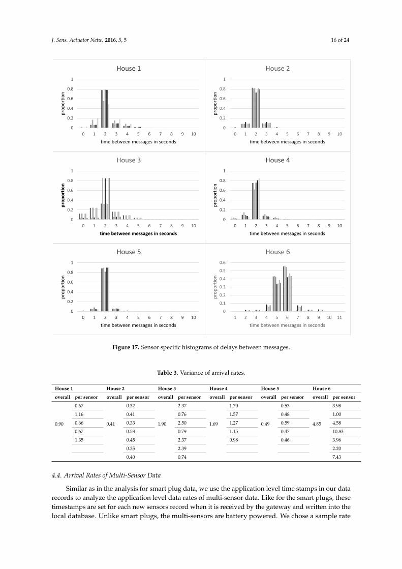
Figure 17 provides more details on the divergence of arrival rates, by drilling down on sensorlevel. As the figure shows, arrival rates of sensor measurements vary among sensors within the samehouse. For instance, in House 1 we observe that three of five sensors have very similar distribution forthe arrival rates of their measurements. However, two sensors differ from that distributions. For thesetwo sensors, the arrival rates divert considerably more from the expected two second interval. Similar,we observe two groups of sensors with similar distributions for arrival rates in House 3. Here, threeof five sensors show similarly distributed and relatively large deviations from the expected value.The other two sensors show only few and small deviations. Compared to each other, the correspondingdistributions for these two sensors are also very similar.
In particular, for House 3 it is notable how the distributions of arrival rates fall in two very distinctgroups. It is therefore likely that the larger deviations in arrival rates have the same or similar causefor all sensors. A possible explanation is multi-hop communication in the ZigBee network. Somesensors have a direct connection to the gateway while others get their messages relayed by a neighborsensor. Communication via one hop is potentially more error prone than direct communication.Another possible explanation is that the different groups of sensors are situated in different physicalconditions. That is, a group of similarly performing sensors may be deployed in the same room, havingto communicate through the same walls to the gateway.
Table 3 provides an overview of the gap distributions of gaps sizes per house and sensor withregards to the variance. Note that we removed rare outliers (i.e., with only a single observation inthe whole data set) from the computation. For the expectation value we took the sample rate of thecorresponding device. In summary, we find that a considerable proportion of sensors shows lowvariance in arrival rates (between 0.32 s and 1 s), while a smaller proportion yields high variance(between 1 s and 10.83 s). Each house has at least one sensor with a variance below or up to one second.However, the overall variance differs significantly due to the different numbers of sensors with highvariances in the deployed portfolio.
J. Sens. Actuator Netw. 2016, 5, 5 16 of 24
J. Sens. Actuator Netw. 2016, 5, 5 15 of 23
these two sensors, the arrival rates divert considerably more from the expected two second interval. Similar, we observe two groups of sensors with similar distributions for arrival rates in House 3. Here, three of five sensors show similarly distributed and relatively large deviations from the expected value. The other two sensors show only few and small deviations. Compared to each other, the corresponding distributions for these two sensors are also very similar.
In particular, for House 3 it is notable how the distributions of arrival rates fall in two very distinct groups. It is therefore likely that the larger deviations in arrival rates have the same or similar cause for all sensors. A possible explanation is multi-hop communication in the ZigBee network. Some sensors have a direct connection to the gateway while others get their messages relayed by a neighbor sensor. Communication via one hop is potentially more error prone than direct communication. Another possible explanation is that the different groups of sensors are situated in different physical conditions. That is, a group of similarly performing sensors may be deployed in the same room, having to communicate through the same walls to the gateway.
Figure 17. Sensor specific histograms of delays between messages.
Table 3 provides an overview of the gap distributions of gaps sizes per house and sensor with regards to the variance. Note that we removed rare outliers (i.e., with only a single observation in the whole data set) from the computation. For the expectation value we took the sample rate of the corresponding device. In summary, we find that a considerable proportion of sensors shows low variance in arrival rates (between 0.32 s and 1 s), while a smaller proportion yields high variance
0
0.1
0.2
0.3
0.4
0.5
0.6
1 2 3 4 5 6 7 8 9 10 11
prop
ortio
n
time between messages in seconds
House 6
0
0.2
0.4
0.6
0.8
1
0 1 2 3 4 5 6 7 8 9 10
prop
ortio
n
time between messages in seconds
House 5
0
0.2
0.4
0.6
0.8
1
0 1 2 3 4 5 6 7 8 9 10
prop
ortio
n
time between messages in seconds
House 4
0
0.2
0.4
0.6
0.8
1
0 1 2 3 4 5 6 7 8 9 10
prop
ortio
n
time between messages in seconds
House 3
0
0.2
0.4
0.6
0.8
1
0 1 2 3 4 5 6 7 8 9 10
prop
ortio
n
time between messages in seconds
House 2
0
0.2
0.4
0.6
0.8
1
0 1 2 3 4 5 6 7 8 9 10
prop
ortio
n
time between messages in seconds
House 1
Figure 17. Sensor specific histograms of delays between messages.
Table 3. Variance of arrival rates.
House 1 House 2 House 3 House 4 House 5 House 6
overall per sensor overall per sensor overall per sensor overall per sensor overall per sensor overall per sensor
0.90
0.67
0.41
0.32
1.90
2.37
1.69
1.70
0.49
0.53
4.85
3.98
1.16 0.41 0.76 1.57 0.48 1.00
0.66 0.33 2.50 1.27 0.59 4.58
0.67 0.58 0.79 1.15 0.47 10.83
1.35 0.45 2.37 0.98 0.46 3.96
0.35 2.39 2.20
0.40 0.74 7.43
4.4. Arrival Rates of Multi-Sensor Data
Similar as in the analysis for smart plug data, we use the application level time stamps in our datarecords to analyze the application level data rates of multi-sensor data. Like for the smart plugs, thesetimestamps are set for each new sensors record when it is received by the gateway and written into thelocal database. Unlike smart plugs, the multi-sensors are battery powered. We chose a sample rate

J. Sens. Actuator Netw. 2016, 5, 5 17 of 24
of one sample every 6 min to ensure a sufficient battery life time (i.e., more than 6 months with oneset of batteries). For all houses we took data from the same month in summer. Like for smart plugs,we compute the recorded time difference between consecutive entries from the same sensor sourceto analyze arrival rates on application level. Under ideal conditions, this delay between consecutivevalues resembles sample rate of the sensor. That is, we expect a new entry every 6 min. To understandhow the actual arrival rates compare to the expected value we count for each observed delay howoften a delay of that length occurs (with a time resolution of one second). Figure 18 visualized theresults as scatter plots.J. Sens. Actuator Netw. 2016, 5, 5 17 of 23
Figure 18. Number of observations of different time gaps between messages.
Figure 19. Cont.
1
10
100
1000
10000
0 1000 2000 3000 4000 5000 6000 7000 8000 9000
num
ber o
f obs
erva
tions
time between messages in seconds
House 1
1
10
100
1000
10000
1 10 100 1000 10000 100000
num
ber o
f obs
erva
tions
time between messages in seconds
House 3
1
10
100
1000
10000
1 10 100 1000 10000nu
mbe
r of o
bser
vatio
ns
time between messages in seconds
House 2
1
10
100
1000
10000
1 10 100 1000 10000 100000
num
ber o
f obs
erva
tions
time between messages in seconds
House 4
1
10
100
1000
10000
1 10 100 1000 10000
num
ber o
f obs
erva
tions
time between messages in seconds
Hosue 5
1
10
100
1000
10000
0 50 100 150 200 250 300 350 400
num
ber o
f obs
erva
tions
time between messages in seconds
House 4
1
10
100
1000
10000
0 50 100 150 200 250 300 350 400
num
ber o
f obs
erva
tions
time between messages in seconds
House 2
1
10
100
1000
10000
0 50 100 150 200 250 300 350 400
num
ber o
f obs
erva
tions
time between messages in seconds
House 3
1
10
100
1000
10000
0 50 100 150 200 250 300 350 400
num
ber o
f obs
erva
tions
time between messages in seconds
House 1
Figure 18. Number of observations of different time gaps between messages.
The x-axis reflects the delay duration and the y-axis marks the observed count for each delay.House 6 is missing from the analysis because no multi-sensors were available in this installation.
As Figure 18 shows, the observed arrival rates differ significantly from the expected 6 min.The delay values with the highest count are about 6 min for all houses (361 s in most cases), but asubstantial number of observations deviate from that value by several seconds or even minutes. Also,in the vicinity of the expected value we observe high counts for values that are several seconds off fromthe expected 6 min. Figure 19 details the analysis of these deviations by zooming in on the time-axis.The figure shows several occurrences where the time between message arrivals is tens of secondsshorter or longer than expected. The order of magnitude and frequency of these deviations is notablyhigher than for the smart plugs.

J. Sens. Actuator Netw. 2016, 5, 5 18 of 24
J. Sens. Actuator Netw. 2016, 5, 5 17 of 23
Figure 18. Number of observations of different time gaps between messages.
Figure 19. Cont.
1
10
100
1000
10000
0 1000 2000 3000 4000 5000 6000 7000 8000 9000
num
ber o
f obs
erva
tions
time between messages in seconds
House 1
1
10
100
1000
10000
1 10 100 1000 10000 100000
num
ber o
f obs
erva
tions
time between messages in seconds
House 3
1
10
100
1000
10000
1 10 100 1000 10000
num
ber o
f obs
erva
tions
time between messages in seconds
House 2
1
10
100
1000
10000
1 10 100 1000 10000 100000
num
ber o
f obs
erva
tions
time between messages in seconds
House 4
1
10
100
1000
10000
1 10 100 1000 10000
num
ber o
f obs
erva
tions
time between messages in seconds
Hosue 5
1
10
100
1000
10000
0 50 100 150 200 250 300 350 400
num
ber o
f obs
erva
tions
time between messages in seconds
House 4
1
10
100
1000
10000
0 50 100 150 200 250 300 350 400
num
ber o
f obs
erva
tions
time between messages in seconds
House 2
1
10
100
1000
10000
0 50 100 150 200 250 300 350 400
num
ber o
f obs
erva
tions
time between messages in seconds
House 3
1
10
100
1000
10000
0 50 100 150 200 250 300 350 400
num
ber o
f obs
erva
tions
time between messages in seconds
House 1
J. Sens. Actuator Netw. 2016, 5, 5 18 of 23
Figure 19. Number of observations of different time gaps between messages, zoomed in on lower values.
4.5. Downtimes of Infrastructure Components
In this section, we analyze the behavior of the gateways during the months they were supposed to be active. Specifically, Figure 20 shows the behavior of each gateway in terms of cumulative number of measurements received per month. As the figure shows, the behavior is very different every month. In order to understand the reason, we report from Figure 21 to Figure 26 also the number of measures received from sensors and smart plugs separately, so this can help us to identify when the gateway was down or when some devices were disconnected from the gateway causing a drop on the measurement count.
Figure 20. Gateways behavior per month.
1
10
100
1000
10000
0 50 100 150 200 250 300 350 400
num
ber o
f obs
erva
tions
time between messages in seconds
House 5
0
5
10
15
20
25
30
35
40
45
Jul-1
3
Aug-
13
Sep-
13
Oct
-13
Nov
-13
Dec-
13
Jan-
14
Feb-
14
Mar
-14
Apr-
14
May
-14
Jun-
14
Jul-1
4
Aug-
14
Sep-
14
Oct
-14
Nov
-14
Dec-
14
Mea
sure
men
ts (c
ount
)M
illio
ns
Date
House 1
0
10
20
30
40
50
60
Sep-
13
Oct
-13
Nov
-13
Dec-
13
Jan-
14
Feb-
14
Mar
-14
Apr-
14
May
-14
Jun-
14
Jul-1
4
Aug-
14
Sep-
14
Oct
-14
Nov
-14
Dec-
14
Jan-
15
Feb-
15
Mea
sure
men
ts (c
ount
)M
illio
ns
Date
House 2
0
10
20
30
40
50
60
Jul-1
3
Aug-
13
Sep-
13
Oct
-13
Nov
-13
Dec-
13
Jan-
14
Feb-
14
Mar
-14
Apr-
14
May
-14
Jun-
14
Jul-1
4
Aug-
14
Sep-
14
Oct
-14
Nov
-14
Dec-
14
Mea
sure
men
ts (c
ount
)M
illio
ns
Date
House 3
0
5
10
15
20
25
30
35
Nov
-13
Dec-
13
Jan-
14
Feb-
14
Mar
-14
Apr-
14
May
-14
Jun-
14
Jul-1
4
Mea
sure
men
ts (c
ount
)M
illio
ns
Date
House 4
0
10
20
30
40
50
60
Feb-
13
Mar
-13
Apr-
13
May
-13
Jun-
13
Jul-1
3
Aug-
13
Sep-
13
Oct
-13
Nov
-13
Dec-
13
Jan-
14
Feb-
14
Mar
-14
Apr-
14
May
-14
Jun-
14
Jul-1
4
Aug-
14
Sep-
14
Oct
-14
Nov
-14
Mea
sure
men
ts (c
ount
)M
illio
ns
Date
House 5
0
0.2
0.4
0.6
0.8
1
1.2
1.4
1.6
1.8
2
Jan-
14
Feb-
14
Mar
-14
Apr-
14
May
-14
Jun-
14
Jul-1
4
Aug-
14
Sep-
14
Oct
-14
Nov
-14
Dec-
14
Mea
sure
men
ts (c
ount
)M
illio
ns
Date
House 6
Figure 19. Number of observations of different time gaps between messages, zoomed in onlower values.
The overview in Figure 18 further reveals that the time spans between consecutive messagesaccumulate around certain values. For House 1, we observe high counts for values that are roughlymultiples of 6 min. Such a pattern is expected as results for lost messages. Notably, House 1 is the onlyhouse were such patterns materialize. For the other houses we do not observe accumulations aroundthe multiples of 6 min. That means, drop rates were overall low in 4 of the 5 analyzed cases. However,at all houses we do find accumulations at values that are not multiples of the sample rate. In particular,some spikes can be seen for values around one minute, 250 s. These patterns cannot be explainedby dropped messages and are assumed to be a result of hardware properties of use sensors. Overall,the analysis shows that time spans between consecutive messages are scattered across large ranges.This leads to rather unstable arrival rates that must be accounted for by applications that use the data.
4.5. Downtimes of Infrastructure Components
In this section, we analyze the behavior of the gateways during the months they were supposedto be active. Specifically, Figure 20 shows the behavior of each gateway in terms of cumulative numberof measurements received per month. As the figure shows, the behavior is very different every month.In order to understand the reason, we report from Figures 21–26 also the number of measures receivedfrom sensors and smart plugs separately, so this can help us to identify when the gateway was downor when some devices were disconnected from the gateway causing a drop on the measurement count.
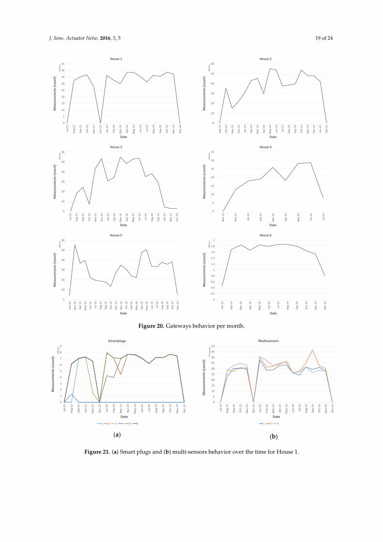
J. Sens. Actuator Netw. 2016, 5, 5 19 of 24
J. Sens. Actuator Netw. 2016, 5, 5 18 of 23
Figure 19. Number of observations of different time gaps between messages, zoomed in on lower values.
4.5. Downtimes of Infrastructure Components
In this section, we analyze the behavior of the gateways during the months they were supposed to be active. Specifically, Figure 20 shows the behavior of each gateway in terms of cumulative number of measurements received per month. As the figure shows, the behavior is very different every month. In order to understand the reason, we report from Figure 21 to Figure 26 also the number of measures received from sensors and smart plugs separately, so this can help us to identify when the gateway was down or when some devices were disconnected from the gateway causing a drop on the measurement count.
Figure 20. Gateways behavior per month.
1
10
100
1000
10000
0 50 100 150 200 250 300 350 400
num
ber o
f obs
erva
tions
time between messages in seconds
House 5
0
5
10
15
20
25
30
35
40
45Ju
l-13
Aug-
13
Sep-
13
Oct
-13
Nov
-13
Dec-
13
Jan-
14
Feb-
14
Mar
-14
Apr-
14
May
-14
Jun-
14
Jul-1
4
Aug-
14
Sep-
14
Oct
-14
Nov
-14
Dec-
14
Mea
sure
men
ts (c
ount
)M
illio
ns
Date
House 1
0
10
20
30
40
50
60
Sep-
13
Oct
-13
Nov
-13
Dec-
13
Jan-
14
Feb-
14
Mar
-14
Apr-
14
May
-14
Jun-
14
Jul-1
4
Aug-
14
Sep-
14
Oct
-14
Nov
-14
Dec-
14
Jan-
15
Feb-
15
Mea
sure
men
ts (c
ount
)M
illio
ns
Date
House 2
0
10
20
30
40
50
60
Jul-1
3
Aug-
13
Sep-
13
Oct
-13
Nov
-13
Dec-
13
Jan-
14
Feb-
14
Mar
-14
Apr-
14
May
-14
Jun-
14
Jul-1
4
Aug-
14
Sep-
14
Oct
-14
Nov
-14
Dec-
14
Mea
sure
men
ts (c
ount
)M
illio
ns
Date
House 3
0
5
10
15
20
25
30
35
Nov
-13
Dec-
13
Jan-
14
Feb-
14
Mar
-14
Apr-
14
May
-14
Jun-
14
Jul-1
4
Mea
sure
men
ts (c
ount
)M
illio
ns
Date
House 4
0
10
20
30
40
50
60
Feb-
13
Mar
-13
Apr-
13
May
-13
Jun-
13
Jul-1
3
Aug-
13
Sep-
13
Oct
-13
Nov
-13
Dec-
13
Jan-
14
Feb-
14
Mar
-14
Apr-
14
May
-14
Jun-
14
Jul-1
4
Aug-
14
Sep-
14
Oct
-14
Nov
-14
Mea
sure
men
ts (c
ount
)M
illio
ns
Date
House 5
0
0.2
0.4
0.6
0.8
1
1.2
1.4
1.6
1.8
2
Jan-
14
Feb-
14
Mar
-14
Apr-
14
May
-14
Jun-
14
Jul-1
4
Aug-
14
Sep-
14
Oct
-14
Nov
-14
Dec-
14
Mea
sure
men
ts (c
ount
)M
illio
ns
Date
House 6
Figure 20. Gateways behavior per month.
J. Sens. Actuator Netw. 2016, 5, 5 19 of 23
Looking at the figures, it is clear that the gateway of House 1 went down in the last part of November till December 2013 maybe due to some power issues or an operating system crash. It was rebooted in January 2014. Apart from Smart Plug 4 (that was on only some days in August 2013 and off all the other months) all the other devices in House 1 reported results with a very close frequency.
House 2 presents a behavior that changes during the months. We note a minimum in November 2013 where the gateway was disconnected for several weeks and all the devices reported a low number of values. The other minimum value was in April 2014 for the same reason. Instead, in August 2014 we observe that both a smart plug and a multi-sensor were disconnected for several days. This can be related to a disconnection in the ZigBee network due to the removal of the smart plug and consequently disconnection of the multi-sensor that used that specific smart plug to reach the gateway.
(a) (b)
Figure 21. (a) Smart plugs and (b) multi-sensors behavior over the time for House 1.
(a) (b)
Figure 22. (a) Smart plugs and (b) multi-sensors behavior over the time for House 2.
(a) (b)
Figure 23. (a) Smart plugs and (b) multi-sensors behavior over the time for House 3.
0
1
2
3
4
5
6
7
8
9
Jul-1
3
Aug-
13
Sep-
13
Oct
-13
Nov
-13
Dec-
13
Jan-
14
Feb-
14
Mar
-14
Apr-
14
May
-14
Jun-
14
Jul-1
4
Aug-
14
Sep-
14
Oct
-14
Nov
-14
Dec-
14
Mea
sure
men
ts (c
ount
)M
illio
ns
Date
Smartplugs
1 2 3 4 5 6
0
5
10
15
20
25
30
35
40
45
50
Jul-1
3
Aug-
13
Sep-
13
Oct
-13
Nov
-13
Dec-
13
Jan-
14
Feb-
14
Mar
-14
Apr-
14
May
-14
Jun-
14
Jul-1
4
Aug-
14
Sep-
14
Oct
-14
Nov
-14
Dec-
14
Mea
sure
men
ts (c
ount
)Th
ousa
nds
Date
Multisensors
1 2 3
0
1
2
3
4
5
6
7
8
9
Sep-
13
Oct
-13
Nov
-13
Dec-
13
Jan-
14
Feb-
14
Mar
-14
Apr-
14
May
-14
Jun-
14
Jul-1
4
Aug-
14
Sep-
14
Oct
-14
Nov
-14
Dec-
14
Jan-
15
Feb-
15
Mea
sure
men
ts (c
ount
)M
illio
ns
Date
Smartplugs
1 2 3 4 5 6 7
0
10
20
30
40
50
60
Sep-
13
Oct
-13
Nov
-13
Dec-
13
Jan-
14
Feb-
14
Mar
-14
Apr-
14
May
-14
Jun-
14
Jul-1
4
Aug-
14
Sep-
14
Oct
-14
Nov
-14
Dec-
14
Jan-
15
Feb-
15
Mea
sure
men
ts (c
ount
) Thou
sand
s
Date
Multisensors
1 2 3 4
0
1
2
3
4
5
6
7
8
9
Jul-1
3
Aug-
13
Sep-
13
Oct
-13
Nov
-13
Dec-
13
Jan-
14
Feb-
14
Mar
-14
Apr-
14
May
-14
Jun-
14
Jul-1
4
Aug-
14
Sep-
14
Oct
-14
Nov
-14
Dec-
14
Mea
sure
men
ts (c
ount
)M
illio
ns
Date
Smartplugs
1 2 3 4 5 6 7
0
5
10
15
20
25
30
35
40
45
50
Jul-1
3
Aug-
13
Sep-
13
Oct
-13
Nov
-13
Dec-
13
Jan-
14
Feb-
14
Mar
-14
Apr-
14
May
-14
Jun-
14
Jul-1
4
Aug-
14
Sep-
14
Oct
-14
Nov
-14
Dec-
14
Mea
sure
men
ts (c
ount
) Thou
sand
s
Date
Multisensors
1 2 3 4
Figure 21. (a) Smart plugs and (b) multi-sensors behavior over the time for House 1.

J. Sens. Actuator Netw. 2016, 5, 5 20 of 24
J. Sens. Actuator Netw. 2016, 5, 5 19 of 23
Looking at the figures, it is clear that the gateway of House 1 went down in the last part of November till December 2013 maybe due to some power issues or an operating system crash. It was rebooted in January 2014. Apart from Smart Plug 4 (that was on only some days in August 2013 and off all the other months) all the other devices in House 1 reported results with a very close frequency.
House 2 presents a behavior that changes during the months. We note a minimum in November 2013 where the gateway was disconnected for several weeks and all the devices reported a low number of values. The other minimum value was in April 2014 for the same reason. Instead, in August 2014 we observe that both a smart plug and a multi-sensor were disconnected for several days. This can be related to a disconnection in the ZigBee network due to the removal of the smart plug and consequently disconnection of the multi-sensor that used that specific smart plug to reach the gateway.
(a) (b)
Figure 21. (a) Smart plugs and (b) multi-sensors behavior over the time for House 1.
(a) (b)
Figure 22. (a) Smart plugs and (b) multi-sensors behavior over the time for House 2.
(a) (b)
Figure 23. (a) Smart plugs and (b) multi-sensors behavior over the time for House 3.
0
1
2
3
4
5
6
7
8
9
Jul-1
3
Aug-
13
Sep-
13
Oct
-13
Nov
-13
Dec-
13
Jan-
14
Feb-
14
Mar
-14
Apr-
14
May
-14
Jun-
14
Jul-1
4
Aug-
14
Sep-
14
Oct
-14
Nov
-14
Dec-
14
Mea
sure
men
ts (c
ount
)M
illio
ns
Date
Smartplugs
1 2 3 4 5 6
0
5
10
15
20
25
30
35
40
45
50
Jul-1
3
Aug-
13
Sep-
13
Oct
-13
Nov
-13
Dec-
13
Jan-
14
Feb-
14
Mar
-14
Apr-
14
May
-14
Jun-
14
Jul-1
4
Aug-
14
Sep-
14
Oct
-14
Nov
-14
Dec-
14
Mea
sure
men
ts (c
ount
)Th
ousa
nds
Date
Multisensors
1 2 3
0
1
2
3
4
5
6
7
8
9Se
p-13
Oct
-13
Nov
-13
Dec-
13
Jan-
14
Feb-
14
Mar
-14
Apr-
14
May
-14
Jun-
14
Jul-1
4
Aug-
14
Sep-
14
Oct
-14
Nov
-14
Dec-
14
Jan-
15
Feb-
15
Mea
sure
men
ts (c
ount
)M
illio
ns
Date
Smartplugs
1 2 3 4 5 6 7
0
10
20
30
40
50
60
Sep-
13
Oct
-13
Nov
-13
Dec-
13
Jan-
14
Feb-
14
Mar
-14
Apr-
14
May
-14
Jun-
14
Jul-1
4
Aug-
14
Sep-
14
Oct
-14
Nov
-14
Dec-
14
Jan-
15
Feb-
15
Mea
sure
men
ts (c
ount
) Thou
sand
s
Date
Multisensors
1 2 3 4
0
1
2
3
4
5
6
7
8
9
Jul-1
3
Aug-
13
Sep-
13
Oct
-13
Nov
-13
Dec-
13
Jan-
14
Feb-
14
Mar
-14
Apr-
14
May
-14
Jun-
14
Jul-1
4
Aug-
14
Sep-
14
Oct
-14
Nov
-14
Dec-
14
Mea
sure
men
ts (c
ount
)M
illio
ns
Date
Smartplugs
1 2 3 4 5 6 7
0
5
10
15
20
25
30
35
40
45
50
Jul-1
3
Aug-
13
Sep-
13
Oct
-13
Nov
-13
Dec-
13
Jan-
14
Feb-
14
Mar
-14
Apr-
14
May
-14
Jun-
14
Jul-1
4
Aug-
14
Sep-
14
Oct
-14
Nov
-14
Dec-
14
Mea
sure
men
ts (c
ount
) Thou
sand
s
Date
Multisensors
1 2 3 4
Figure 22. (a) Smart plugs and (b) multi-sensors behavior over the time for House 2.
J. Sens. Actuator Netw. 2016, 5, 5 19 of 23
Looking at the figures, it is clear that the gateway of House 1 went down in the last part of November till December 2013 maybe due to some power issues or an operating system crash. It was rebooted in January 2014. Apart from Smart Plug 4 (that was on only some days in August 2013 and off all the other months) all the other devices in House 1 reported results with a very close frequency.
House 2 presents a behavior that changes during the months. We note a minimum in November 2013 where the gateway was disconnected for several weeks and all the devices reported a low number of values. The other minimum value was in April 2014 for the same reason. Instead, in August 2014 we observe that both a smart plug and a multi-sensor were disconnected for several days. This can be related to a disconnection in the ZigBee network due to the removal of the smart plug and consequently disconnection of the multi-sensor that used that specific smart plug to reach the gateway.
(a) (b)
Figure 21. (a) Smart plugs and (b) multi-sensors behavior over the time for House 1.
(a) (b)
Figure 22. (a) Smart plugs and (b) multi-sensors behavior over the time for House 2.
(a) (b)
Figure 23. (a) Smart plugs and (b) multi-sensors behavior over the time for House 3.
0
1
2
3
4
5
6
7
8
9
Jul-1
3
Aug-
13
Sep-
13
Oct
-13
Nov
-13
Dec-
13
Jan-
14
Feb-
14
Mar
-14
Apr-
14
May
-14
Jun-
14
Jul-1
4
Aug-
14
Sep-
14
Oct
-14
Nov
-14
Dec-
14
Mea
sure
men
ts (c
ount
)M
illio
ns
Date
Smartplugs
1 2 3 4 5 6
0
5
10
15
20
25
30
35
40
45
50
Jul-1
3
Aug-
13
Sep-
13
Oct
-13
Nov
-13
Dec-
13
Jan-
14
Feb-
14
Mar
-14
Apr-
14
May
-14
Jun-
14
Jul-1
4
Aug-
14
Sep-
14
Oct
-14
Nov
-14
Dec-
14
Mea
sure
men
ts (c
ount
)Th
ousa
nds
Date
Multisensors
1 2 3
0
1
2
3
4
5
6
7
8
9Se
p-13
Oct
-13
Nov
-13
Dec-
13
Jan-
14
Feb-
14
Mar
-14
Apr-
14
May
-14
Jun-
14
Jul-1
4
Aug-
14
Sep-
14
Oct
-14
Nov
-14
Dec-
14
Jan-
15
Feb-
15
Mea
sure
men
ts (c
ount
)M
illio
ns
Date
Smartplugs
1 2 3 4 5 6 7
0
10
20
30
40
50
60
Sep-
13
Oct
-13
Nov
-13
Dec-
13
Jan-
14
Feb-
14
Mar
-14
Apr-
14
May
-14
Jun-
14
Jul-1
4
Aug-
14
Sep-
14
Oct
-14
Nov
-14
Dec-
14
Jan-
15
Feb-
15
Mea
sure
men
ts (c
ount
) Thou
sand
s
Date
Multisensors
1 2 3 4
0
1
2
3
4
5
6
7
8
9
Jul-1
3
Aug-
13
Sep-
13
Oct
-13
Nov
-13
Dec-
13
Jan-
14
Feb-
14
Mar
-14
Apr-
14
May
-14
Jun-
14
Jul-1
4
Aug-
14
Sep-
14
Oct
-14
Nov
-14
Dec-
14
Mea
sure
men
ts (c
ount
)M
illio
ns
Date
Smartplugs
1 2 3 4 5 6 7
0
5
10
15
20
25
30
35
40
45
50
Jul-1
3
Aug-
13
Sep-
13
Oct
-13
Nov
-13
Dec-
13
Jan-
14
Feb-
14
Mar
-14
Apr-
14
May
-14
Jun-
14
Jul-1
4
Aug-
14
Sep-
14
Oct
-14
Nov
-14
Dec-
14
Mea
sure
men
ts (c
ount
) Thou
sand
s
Date
Multisensors
1 2 3 4
Figure 23. (a) Smart plugs and (b) multi-sensors behavior over the time for House 3.J. Sens. Actuator Netw. 2016, 5, 5 20 of 23
(a) (b)
Figure 24. (a) Smart plugs and (b) multi-sensors behavior over the time for House 4.
The Gateway of House 3 was down three weeks in October 2013, then it was rebooted. In January and February 2014, it was on only for half of the time. Also in this case the motivation can be a power failure or a crash in the operating system. We note also that, in August and September 2013, the data collected are less with respect to the other months. This can be due to a not very stable connection of the network at the beginning. The same happened in September and October 2014 before dismissing the Gateway, due to the fact that probably the user started to disconnect the smart plugs causing a disruption in the ZigBee network.
(a) (b)
Figure 25. (a) Smart plugs and (b) multi-sensors behavior over the time for House 5.
Figure 26. Smart plugs behavior over the time for House 6.
0
1
2
3
4
5
6
7
8
9
Nov
-13
Dec-
13
Jan-
14
Feb-
14
Mar
-14
Apr-
14
May
-14
Jun-
14
Jul-1
4
Mea
sure
men
ts (c
ount
)M
illio
ns
Date
Smartplugs
1 2 3 4 5 6 7
0
10
20
30
40
50
60
70
80
Nov
-13
Dec-
13
Jan-
14
Feb-
14
Mar
-14
Apr-
14
May
-14
Jun-
14
Jul-1
4
Mea
sure
men
ts (c
ount
) Thou
sand
s
Date
Multisensors
1 2 3
0
1
2
3
4
5
6
7
8
9
Feb-
13
Mar
-13
Apr-
13
May
-13
Jun-
13
Jul-1
3
Aug-
13
Sep-
13
Oct
-13
Nov
-13
Dec-
13
Jan-
14
Feb-
14
Mar
-14
Apr-
14
May
-14
Jun-
14
Jul-1
4
Aug-
14
Sep-
14
Oct
-14
Nov
-14
Mea
sure
men
ts (c
ount
)M
illio
ns
Date
Smartplugs
1 2 3 4 5 6 7
0
10
20
30
40
50
60
70
Feb-
13
Mar
-13
Apr-
13
May
-13
Jun-
13
Jul-1
3
Aug-
13
Sep-
13
Oct
-13
Nov
-13
Dec-
13
Jan-
14
Feb-
14
Mar
-14
Apr-
14
May
-14
Jun-
14
Jul-1
4
Aug-
14
Sep-
14
Oct
-14
Nov
-14
Mea
sure
men
ts (c
ount
) Thou
sand
s
Date
Multisensors
1 2 3 4
0
50
100
150
200
250
300
Jan-
14
Feb-
14
Mar
-14
Apr-
14
May
-14
Jun-
14
Jul-1
4
Aug-
14
Sep-
14
Oct
-14
Nov
-14
Dec-
14
Mea
sure
men
ts (c
ount
) Thou
sand
s
Date
Smartplugs
1 2 3 4 5 6 7
Figure 24. (a) Smart plugs and (b) multi-sensors behavior over the time for House 4.
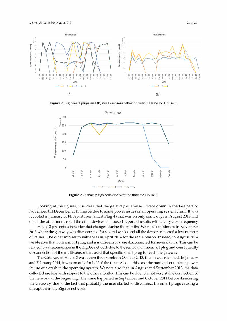
J. Sens. Actuator Netw. 2016, 5, 5 21 of 24
J. Sens. Actuator Netw. 2016, 5, 5 20 of 23
(a) (b)
Figure 24. (a) Smart plugs and (b) multi-sensors behavior over the time for House 4.
The Gateway of House 3 was down three weeks in October 2013, then it was rebooted. In January and February 2014, it was on only for half of the time. Also in this case the motivation can be a power failure or a crash in the operating system. We note also that, in August and September 2013, the data collected are less with respect to the other months. This can be due to a not very stable connection of the network at the beginning. The same happened in September and October 2014 before dismissing the Gateway, due to the fact that probably the user started to disconnect the smart plugs causing a disruption in the ZigBee network.
(a) (b)
Figure 25. (a) Smart plugs and (b) multi-sensors behavior over the time for House 5.
Figure 26. Smart plugs behavior over the time for House 6.
0
1
2
3
4
5
6
7
8
9
Nov
-13
Dec-
13
Jan-
14
Feb-
14
Mar
-14
Apr-
14
May
-14
Jun-
14
Jul-1
4
Mea
sure
men
ts (c
ount
)M
illio
ns
Date
Smartplugs
1 2 3 4 5 6 7
0
10
20
30
40
50
60
70
80
Nov
-13
Dec-
13
Jan-
14
Feb-
14
Mar
-14
Apr-
14
May
-14
Jun-
14
Jul-1
4
Mea
sure
men
ts (c
ount
) Thou
sand
s
Date
Multisensors
1 2 3
0
1
2
3
4
5
6
7
8
9Fe
b-13
Mar
-13
Apr-
13
May
-13
Jun-
13
Jul-1
3
Aug-
13
Sep-
13
Oct
-13
Nov
-13
Dec-
13
Jan-
14
Feb-
14
Mar
-14
Apr-
14
May
-14
Jun-
14
Jul-1
4
Aug-
14
Sep-
14
Oct
-14
Nov
-14
Mea
sure
men
ts (c
ount
)M
illio
ns
Date
Smartplugs
1 2 3 4 5 6 7
0
10
20
30
40
50
60
70
Feb-
13
Mar
-13
Apr-
13
May
-13
Jun-
13
Jul-1
3
Aug-
13
Sep-
13
Oct
-13
Nov
-13
Dec-
13
Jan-
14
Feb-
14
Mar
-14
Apr-
14
May
-14
Jun-
14
Jul-1
4
Aug-
14
Sep-
14
Oct
-14
Nov
-14
Mea
sure
men
ts (c
ount
) Thou
sand
s
Date
Multisensors
1 2 3 4
0
50
100
150
200
250
300
Jan-
14
Feb-
14
Mar
-14
Apr-
14
May
-14
Jun-
14
Jul-1
4
Aug-
14
Sep-
14
Oct
-14
Nov
-14
Dec-
14
Mea
sure
men
ts (c
ount
) Thou
sand
s
Date
Smartplugs
1 2 3 4 5 6 7
Figure 25. (a) Smart plugs and (b) multi-sensors behavior over the time for House 5.
J. Sens. Actuator Netw. 2016, 5, 5 20 of 23
(a) (b)
Figure 24. (a) Smart plugs and (b) multi-sensors behavior over the time for House 4.
The Gateway of House 3 was down three weeks in October 2013, then it was rebooted. In January and February 2014, it was on only for half of the time. Also in this case the motivation can be a power failure or a crash in the operating system. We note also that, in August and September 2013, the data collected are less with respect to the other months. This can be due to a not very stable connection of the network at the beginning. The same happened in September and October 2014 before dismissing the Gateway, due to the fact that probably the user started to disconnect the smart plugs causing a disruption in the ZigBee network.
(a) (b)
Figure 25. (a) Smart plugs and (b) multi-sensors behavior over the time for House 5.
Figure 26. Smart plugs behavior over the time for House 6.
0
1
2
3
4
5
6
7
8
9
Nov
-13
Dec-
13
Jan-
14
Feb-
14
Mar
-14
Apr-
14
May
-14
Jun-
14
Jul-1
4
Mea
sure
men
ts (c
ount
)M
illio
ns
Date
Smartplugs
1 2 3 4 5 6 7
0
10
20
30
40
50
60
70
80
Nov
-13
Dec-
13
Jan-
14
Feb-
14
Mar
-14
Apr-
14
May
-14
Jun-
14
Jul-1
4
Mea
sure
men
ts (c
ount
) Thou
sand
s
Date
Multisensors
1 2 3
0
1
2
3
4
5
6
7
8
9Fe
b-13
Mar
-13
Apr-
13
May
-13
Jun-
13
Jul-1
3
Aug-
13
Sep-
13
Oct
-13
Nov
-13
Dec-
13
Jan-
14
Feb-
14
Mar
-14
Apr-
14
May
-14
Jun-
14
Jul-1
4
Aug-
14
Sep-
14
Oct
-14
Nov
-14
Mea
sure
men
ts (c
ount
)M
illio
ns
Date
Smartplugs
1 2 3 4 5 6 7
0
10
20
30
40
50
60
70
Feb-
13
Mar
-13
Apr-
13
May
-13
Jun-
13
Jul-1
3
Aug-
13
Sep-
13
Oct
-13
Nov
-13
Dec-
13
Jan-
14
Feb-
14
Mar
-14
Apr-
14
May
-14
Jun-
14
Jul-1
4
Aug-
14
Sep-
14
Oct
-14
Nov
-14
Mea
sure
men
ts (c
ount
) Thou
sand
s
Date
Multisensors
1 2 3 4
0
50
100
150
200
250
300
Jan-
14
Feb-
14
Mar
-14
Apr-
14
May
-14
Jun-
14
Jul-1
4
Aug-
14
Sep-
14
Oct
-14
Nov
-14
Dec-
14
Mea
sure
men
ts (c
ount
) Thou
sand
s
Date
Smartplugs
1 2 3 4 5 6 7
Figure 26. Smart plugs behavior over the time for House 6.
Looking at the figures, it is clear that the gateway of House 1 went down in the last part ofNovember till December 2013 maybe due to some power issues or an operating system crash. It wasrebooted in January 2014. Apart from Smart Plug 4 (that was on only some days in August 2013 andoff all the other months) all the other devices in House 1 reported results with a very close frequency.
House 2 presents a behavior that changes during the months. We note a minimum in November2013 where the gateway was disconnected for several weeks and all the devices reported a low numberof values. The other minimum value was in April 2014 for the same reason. Instead, in August 2014we observe that both a smart plug and a multi-sensor were disconnected for several days. This can berelated to a disconnection in the ZigBee network due to the removal of the smart plug and consequentlydisconnection of the multi-sensor that used that specific smart plug to reach the gateway.
The Gateway of House 3 was down three weeks in October 2013, then it was rebooted. In Januaryand February 2014, it was on only for half of the time. Also in this case the motivation can be a powerfailure or a crash in the operating system. We note also that, in August and September 2013, the datacollected are less with respect to the other months. This can be due to a not very stable connection ofthe network at the beginning. The same happened in September and October 2014 before dismissingthe Gateway, due to the fact that probably the user started to disconnect the smart plugs causing adisruption in the ZigBee network.
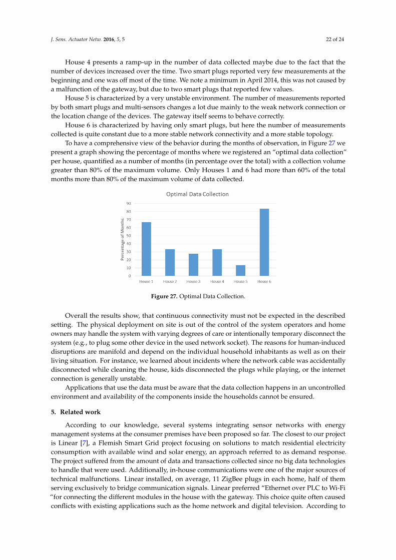
J. Sens. Actuator Netw. 2016, 5, 5 22 of 24
House 4 presents a ramp-up in the number of data collected maybe due to the fact that thenumber of devices increased over the time. Two smart plugs reported very few measurements at thebeginning and one was off most of the time. We note a minimum in April 2014, this was not caused bya malfunction of the gateway, but due to two smart plugs that reported few values.
House 5 is characterized by a very unstable environment. The number of measurements reportedby both smart plugs and multi-sensors changes a lot due mainly to the weak network connection orthe location change of the devices. The gateway itself seems to behave correctly.
House 6 is characterized by having only smart plugs, but here the number of measurementscollected is quite constant due to a more stable network connectivity and a more stable topology.
To have a comprehensive view of the behavior during the months of observation, in Figure 27 wepresent a graph showing the percentage of months where we registered an “optimal data collection”per house, quantified as a number of months (in percentage over the total) with a collection volumegreater than 80% of the maximum volume. Only Houses 1 and 6 had more than 60% of the totalmonths more than 80% of the maximum volume of data collected.
J. Sens. Actuator Netw. 2016, 5, 5 21 of 23
House 4 presents a ramp-up in the number of data collected maybe due to the fact that the number of devices increased over the time. Two smart plugs reported very few measurements at the beginning and one was off most of the time. We note a minimum in April 2014, this was not caused by a malfunction of the gateway, but due to two smart plugs that reported few values.
House 5 is characterized by a very unstable environment. The number of measurements reported by both smart plugs and multi-sensors changes a lot due mainly to the weak network connection or the location change of the devices. The gateway itself seems to behave correctly.
House 6 is characterized by having only smart plugs, but here the number of measurements collected is quite constant due to a more stable network connectivity and a more stable topology.
To have a comprehensive view of the behavior during the months of observation, in Figure 27 we present a graph showing the percentage of months where we registered an “optimal data collection” per house, quantified as a number of months (in percentage over the total) with a collection volume greater than 80% of the maximum volume. Only Houses 1 and 6 had more than 60% of the total months more than 80% of the maximum volume of data collected.
Figure 27. Optimal Data Collection.
Overall the results show, that continuous connectivity must not be expected in the described setting. The physical deployment on site is out of the control of the system operators and home owners may handle the system with varying degrees of care or intentionally temporary disconnect the system (e.g., to plug some other device in the used network socket). The reasons for human-induced disruptions are manifold and depend on the individual household inhabitants as well as on their living situation. For instance, we learned about incidents where the network cable was accidentally disconnected while cleaning the house, kids disconnected the plugs while playing, or the internet connection is generally unstable.
Applications that use the data must be aware that the data collection happens in an uncontrolled environment and availability of the components inside the households cannot be ensured.
5. Related work
According to our knowledge, several systems integrating sensor networks with energy management systems at the consumer premises have been proposed so far. The closest to our project is Linear [7], a Flemish Smart Grid project focusing on solutions to match residential electricity consumption with available wind and solar energy, an approach referred to as demand response. The project suffered from the amount of data and transactions collected since no big data technologies to handle that were used. Additionally, in-house communications were one of the major sources of technical malfunctions. Linear installed, on average, 11 ZigBee plugs in each home, half of them serving exclusively to bridge communication signals. Linear preferred “Ethernet over PLC to Wi-Fi “for connecting the different modules in the house with the gateway. This choice quite often caused conflicts with existing applications such as the home network and digital television. According to the Linear support team, “some families were so excited about the possibilities of the Home Energy Management System that they started moving plugs to different locations in order to trace standby
Figure 27. Optimal Data Collection.
Overall the results show, that continuous connectivity must not be expected in the describedsetting. The physical deployment on site is out of the control of the system operators and homeowners may handle the system with varying degrees of care or intentionally temporary disconnect thesystem (e.g., to plug some other device in the used network socket). The reasons for human-induceddisruptions are manifold and depend on the individual household inhabitants as well as on theirliving situation. For instance, we learned about incidents where the network cable was accidentallydisconnected while cleaning the house, kids disconnected the plugs while playing, or the internetconnection is generally unstable.
Applications that use the data must be aware that the data collection happens in an uncontrolledenvironment and availability of the components inside the households cannot be ensured.
5. Related work
According to our knowledge, several systems integrating sensor networks with energymanagement systems at the consumer premises have been proposed so far. The closest to our projectis Linear [7], a Flemish Smart Grid project focusing on solutions to match residential electricityconsumption with available wind and solar energy, an approach referred to as demand response.The project suffered from the amount of data and transactions collected since no big data technologiesto handle that were used. Additionally, in-house communications were one of the major sources oftechnical malfunctions. Linear installed, on average, 11 ZigBee plugs in each home, half of themserving exclusively to bridge communication signals. Linear preferred “Ethernet over PLC to Wi-Fi“for connecting the different modules in the house with the gateway. This choice quite often causedconflicts with existing applications such as the home network and digital television. According to

J. Sens. Actuator Netw. 2016, 5, 5 23 of 24
the Linear support team, “some families were so excited about the possibilities of the Home EnergyManagement System that they started moving plugs to different locations in order to trace standbylosses, not being aware that they were messing up the network to the extent that the fridge plug startedshowing the behavior of a television in our databases”. Similar issues have been experienced also inour pilot as described earlier.
Another set of related projects was conducted as part of the e-energy funding scheme of theGerman government [8]. For instance, the MeRegio conducted a pilot, mainly focused on using smartmeter data [9] and the project Smart Watts addresses the development of communication standards [10].However, to our knowledge, none of these projects provide detailed insights on the data quality aspectfor smart home applications.
In [11], the authors evaluate the performance of an in-home energy management system based ona ZigBee wireless sensor network. The focus there is the performance of the system on the applicationlevel, meaning the investigation of the potential of both energy management and demand management.The evaluation that has been performed by the authors is based on simulation results, and not on realnetwork deployments in households as in our work.
In [12], energy management in homes has been investigated on a pilot consisting of only threehouseholds in Sacramento. The solution has been implemented using off-the-shelf components basedon power line communication, and it included a web-based monitoring and control of home appliances.Similarly, the MIT provides a detailed dataset with plug-level energy data [13]. However, the dataset isdesigned to drive research on energy disaggregation and not to understand data quality issues underrealistic conditions. Also, it is limited to a few weeks of recorded data.
In [14], the authors present experiences from a pilot study carried out in Norway, focusing ondaily demand response from households, utilizing smart metering, remote load control, pricing basedon the hourly spot price combined with a time of day network tariff, and a token provided to thecustomers indicating peak hours. The pilot study has shown that household customers through simpleand predictable means can adapt their electricity demand to the market situation.
6. Conclusion and Lessons Learned
In this paper, we have provided insights from a three year pilot with a cloud-based test bed forcapturing and analyzing smart-home data. Our results include findings on real-world challengesin the application domain as well as our learnings regarding the data quality issues we have faced.The key challenge that we came across was data loss and reduced data quality on several layers ofour cloud-based architecture. In many cases, the issues are inherent to the application domain whichwe were addressing (home environments) where users intentionally or unintentionally interfere withthe operations of the system, but apart from this unavoidable problem we have presented a detailedanalysis of the main causes that are responsible for data quality related issues.
In our tests, we quantify the data quality of a real-world smart home deployments and show howerrors in such an environment are characterized. The derived characteristics concern (a) data errors;(b) arrival rates; and (c) behavior over time. Regarding (a) data errors we found that these occur onlyrarely. For instance, only 0.004% of measured work values showed a detectable anomaly. However,due to the overall high number of measurements, the total amount false data reaches high numbers.For instance, overall 17.876 faulty values were detected in the measurements of work.
Regarding (b) arrival rates for smart plug data we found significant variations across sensors.The analysis show variance values between about 0.32 and 2.5, for plugs with a sample frequencyof 2 s. For the setup with sampling once per minute, we observe a variance of about 4.9. The overallvariance differs significantly (i.e., between 0.49 and 4.85 s). However, we found in each house sensorswith low variance (i.e., up to 1 s). Thus, we can conclude that ideal communication conditions allowfor low variance in arrival rates, yet most real world setup will cause high variance in data arrival forat least some sensors in the portfolio.

J. Sens. Actuator Netw. 2016, 5, 5 24 of 24
Regarding (c) system behavior over time, we found that under real world conditions data qualitychanges considerably over time. We observe several drops in the overall measurement rate, both onthe gateway and on the sensors level. Overall, only a third of the analyzed houses close to optimalreporting rates more than 60% of the time.
Overall, our work shows researchers as well as practitioners in the smart grid domain whatchallenges they have to expect when integration smart home technology and provide quantifiedinsights into data quality in that domain. The findings support the design of systems and applicationsthat cope with the data challenges and fuel future research on improving data quality for smart homes.
Acknowledgments: This work was enabled through the PeerEnergyCloud that was funded by the FederalMinistry for Economic Affairs and Energy. The authors declare no conflict of interest. The work presented in thispaper was (partly) funded by the H2020 project HOBBIT under the grant agreement number 688227.
Author Contributions: Alessandro Lenoardi, Panayotis Kikiras and Holger Ziekow participated in thePeerEnergyCloud project and worked on the infrastructure for data collection as well as on the executionof the pilot. Martin Strohbach worked on the provisioning of the infrastructure for big data analytics. All authorsconducted the data analysis and provided the corresponding descriptions in the paper.
Conflicts of Interest: The authors declare no conflict of interest.
References
1. Peer Energy Cloud Project. Available online: http://www.peerenergycloud.de (accessed on 16 February 2016).2. Siano, P. Demand response and smart grids—A survey. Renew. Sustain. Energy Rev. 2014, 30, 461–478.
[CrossRef]3. Ziekow, H.; Goebel, C.; Struker, J.; Jacobsen, H.A. The potential of smart home sensors in forecasting
household electricity demand. In Proceedings of the 2013 IEEE International Conference on Smart GridCommunications (SmartGridComm), Vancouver, BC, Canada, 21–24 October 2013; pp. 229–234.
4. The ZigBee Alliance. Available online: http://www.zigbee.org/ (accessed on 5 December 2015).5. Ebinger, P.; Ramos, J.H.; Kikiras, P.; Lischka, M.; Wiesmaier, A. Privacy in smart metering ecosystems.
In Smart Grid Security; Cuellar, J., Ed.; Springer: Berlin/Heidelberg, Germany, 2013; Volume 7823, pp. 120–131.6. Ziekow, H.; Doblander, C.; Goebel, C.; Jacobsen, H.A. Forecasting household electricity demand with
complex event processing: insights from a prototypical solution. In Proceedings of the Industrial Track ofthe 13th ACM/IFIP/USENIX International Middleware Conference, Beijing, China, 9–13 December 2013.
7. Linear. Available online: http://www.linear-smartgrid.be/ (accessed on 5 December 2015).8. Picot, A.; Neumann, K.H. E-Energy; Springer Science & Business Media: Medford, MA, USA, 2009.9. MeRegio. Available online: http://www.digitale-technologien.de/DT/Redaktion/DE/Downloads/
Factsheets/factsheet-meregio.pdf (accessed on 21 December 2015).10. Smart Watts. Available online: http://www.digitale-technologien.de/DT/Redaktion/DE/Downloads/
Factsheets/factsheet-smart-watts.pdf (accessed on 21 December 2015).11. Erol-Kantarci, M.; Mouftah, H.T. Wireless sensor networks for cost-efficient residential energy management
in the smart grid. IEEE Trans. Smart Grid 2011, 2, 314–325. [CrossRef]12. Williams, E.; Matthews, S.; Breton, M.; Brady, T. Use of a computer-based system to measure and manage
energy consumption in the home. In Proceedings of the 2006 IEEE International Symposium on Electronicsand the Environment, Scottsdale, AZ, USA, 8–11 May 2006; pp. 167–172.
13. Kolter, J.Z.; Johnson, M.J. REDD: A Public Data Set for Energy Disaggregation Research. Available online:http://citeseerx.ist.psu.edu/viewdoc/download?doi=10.1.1.454.5796&rep=rep1&type=pdf (accessed on 16February 2016).
14. Saele, H.; Grande, O. Demand response from household customers: Experiences from a pilot study inNorway. IEEE Trans. Smart Grid 2011, 2, 102–109. [CrossRef]
© 2016 by the authors; licensee MDPI, Basel, Switzerland. This article is an open accessarticle distributed under the terms and conditions of the Creative Commons by Attribution(CC-BY) license (http://creativecommons.org/licenses/by/4.0/).