Day 2: Optimization (continued)

1

Presenter: Auralee Edelen

Day 2

1st and 2nd Order Optimization Methods

1st Order Methods:

• Use information about the 1st derivative • Gradient descent and variants (yesterday’s lecture)

→ how to improve choices of step-size and direction?

(and in turn improve sample-efficiency in convergence)

2nd Order Methods:

• Use information about the curvature (2nd derivative)

→ calculate or approximate the Hessian

• Pro: Better direction and step-size than gradient descent

• Con: More costly per iteration to compute

“1.5 Order” Methods:

• In between 1st and 2nd order

• e.g. Powell’s conjugate gradient method

1st and 2nd Order Optimization Methods

1st Order Methods:

• Use information about the 1st derivative • Gradient descent and variants (yesterday’s lecture)

→ how to improve choices of step-size and direction?

(and in turn improve sample-efficiency in convergence)

2nd Order Methods:

• Use information about the curvature (2nd derivative)

→ calculate or approximate the Hessian

• Pro: Better direction and step-size than gradient descent

• Con: More costly per iteration to compute

“1.5 Order” Methods:

• In between 1st and 2nd order

• e.g. Powell’s conjugate gradient method

1st and 2nd Order Optimization Methods

1st Order Methods:

• Use information about the 1st derivative • Gradient descent and variants (yesterday’s lecture)

→ how to improve choices of step-size and direction?

(and in turn improve sample-efficiency in convergence)

2nd Order Methods:

• Use information about the curvature (2nd derivative)

→ calculate or approximate the Hessian

• Pro: Better direction and step-size than gradient descent

• Con: More costly per iteration to compute

“1.5 Order” Methods:

• In between 1st and 2nd order

• e.g. Powell’s conjugate gradient method

Determining the next point: line search

Line search methods define a direction and then do optimization over that line

→ often used as one step in a larger algorithm (e.g. for determining next point)

→ often do not require derivatives

e.g. Brent’s Method:

1. Bracket the minimum

2. Approximate parabola through successive points or use golden section search

3. Iterate

Illustration of Brent’s method from Numerical Recipes

More details: Brent, R. P. Ch. 3-4 in Algorithms for Minimization Without Derivatives. Englewood Cliffs, NJ: Prentice-Hall, 1973.

Example: Powell’s Conjugate Gradient Method

Steps in Powell’s Method:

1. Pick x1

and two directions d1 and d

2

2. Start at x1 and do line search along d

1 to find minimum x

2

3. Start at x2

and do line search along d2 to find x

3

4. Connect x1 to x

3 to define d

3

5. Start at x3 and do line search along d

3 to find x

4

6. Start at x4

and do line search along d2 to find x

4

x1

x2

x3

x4

x5

d1

d2

d3

d2

d3

d4

Does not require derivatives, efficient with regard to direction searched

Robust Conjugate Direction Search (RCDS)

RCDS combines a noise-aware line search with Powell’s method

More details: X. Huang et al, Nucl. Instr. Methods, A 726 (2013) 77-83, https://www.slac.stanford.edu/pubs/slacpubs/15250/slac-pub-15414.pdf

● Designed to deal with noisy online optimization in accelerators → optimization algorithm needs to be sample-efficient, robust to noise

● Was developed for optimization of storage rings (e.g. dynamic aperture, emittance); has since been widely applied in accelerators

● Uses a random sample to find the bounds in each line search, ensuring these are above a specified noise level, and fills in values until an appropriate fit is obtained

Powell Simplex RCDS

Powell’s method not robust with noise simplex does not reach expected minima

2nd Order Methods: Newton’s method

Analogy to root finding

x1x2x3

Taylor series approximation:

Set to 0 to find roots of function:

Iterate:

2nd Order Methods: Newton’s method

Analogy to root finding

x1x2x3

Taylor series approximation:

Set to 0 to find roots of function:

Iterate:

For optimization, take the derivative of the Taylor series

x1x2x3

In essence: Newton’s method iteratively approximates the function with a parabola

2nd Order Methods: Newton’s method

● Pro: better convergence per step than gradient descent

● Con: poor computational scalability O(n3)

→ computing hessian and inverse

● Quasi-Newton methods approximate the Hessian for better scalability (e.g. L-BFGS)

Ryan Tibshirani

black - gradient descentblue - Newton’s method

Multi-Objective Optimization: Intro

Instead of a single objective, in multi-objective optimization (MOO) we want to optimize multiple objectives

Multi-Objective Optimization: Intro

Instead of a single objective, in multi-objective optimization (MOO) we want to optimize multiple objectives

Multi-Objective Optimization: Intro

Instead of a single objective, in multi-objective optimization (MOO) we want to optimize multiple objectives

Multi-Objective Optimization: Intro

Instead of a single objective, in multi-objective optimization (MOO) we want to optimize multiple objectives

Multi-Objective Optimization: Intro

Instead of a single objective, in multi-objective optimization (MOO) we want to optimize multiple objectives

Multi-Objective Optimization: Intro

Instead of a single objective, in multi-objective optimization (MOO) we want to optimize multiple objectives

Multi-Objective Optimization: Dominance

Solutions in single-objective optimization are easy to compare by looking at the objective function values

In multi-objective optimization, solutions are evaluated by the dominance wrt the combinations of objectives

f2(x)

(minimize)

1

2

3

4

f1(x)

(minimize)

5

Solution x1 is said to dominate solution x2 if both of the following are true:

1. x1 is no worse than x2 for all objectives

2. x1 is strictly better than x2 in at least one objective

Multi-Objective Optimization: Dominance

Solutions in single-objective optimization are easy to compare by looking at the objective function values

In multi-objective optimization, solutions are evaluated by the dominance wrt the combinations of objectives

f2(x)

(minimize)

1

2

3

4

f1(x)

(minimize)

5

Solution x1 is said to dominate solution x2 if both of the following are true:

1. x1 is no worse than x2 for all objectives

2. x1 is strictly better than x2 in at least one objective

In this example: 2 dominates 3 4 dominates 5 2 dominates 5 Neither 1 nor 2 dominate each other

Multi-Objective Optimization: Pareto Front

• Non-dominated solution set: all solutions which are not dominated

• Pareto-optimal set: non-dominated solution set over the entire decision space

• Pareto-optimal front: boundary mapped out by Pareto-optimal set

→ For any point on the Pareto front, one cannot improve the value of one objective without reducing another

f2(x)

(minimize)

f1(x)

(minimize)

Reference point

Pareto-optimal front

hypervolume

x2

x1

Example shown is 2D for visualization, but can in principle go up to N-D

feasible objective space feasible design (or “decision”) space

Pareto-optimal solutions

Multi-Objective Optimization: Pareto Front

https://en.wikipedia.org/wiki/File:Zitzler-Deb-Thiele%27s_function_3.pdf

Can also have more complicated Pareto fronts that provide additional challenges (e.g. disconnected regions)

Numerous standard “test functions” are used to assess optimization problems (including multi-objective and constrained optimization)

e.g. see:

Deb et al., Scalable multi-objective optimization test problems, https://ieeexplore.ieee.org/stamp/stamp.jsp?tp=&arnumber=1007032

Husband et al., A review of multiobjective test problems and a scalable test problem toolkit, https://ieeexplore.ieee.org/document/1705400

Wikipedia page on test functions for optimization: https://en.wikipedia.org/wiki/Test_functions_for_optimization

ZDT-3

Multi-Objective Optimization: Scalarization

Scalarization: convert multiple objectives to a single objective

Pro: simple to implement

Con: for a given set of weights one gets only one solution

→ Need to solve optimization problem multiple times with scan through different weights to obtain the Pareto-optimal front

Can be time-consuming and difficult for each optimization to navigate to the front → motivation for population based methods (parallel search)

for k objectives

(linear scalarization)

K. Deb et al

Example of MOO with scalarization: AWAKE electron beam line

Scheinker et al., “Online Multi-Objective Particle Accelerator Optimization of the AWAKE Electron Beam Line for Simultaneous Emittance and Orbit Control” (2020)https://arxiv.org/abs/2003.11155v1

Goal: maintain beam on a target trajectory while minimizing beam size

Uses multi-objective optimization with scalarization. In this case, no need to find the Pareto front!

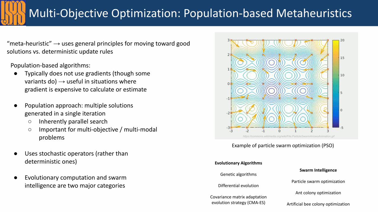
Multi-Objective Optimization: Population-based Metaheuristics

Population-based algorithms:● Typically does not use gradients (though some

variants do) → useful in situations where gradient is expensive to calculate or estimate

● Population approach: multiple solutions generated in a single iteration○ Inherently parallel search○ Important for multi-objective / multi-modal

problems

● Uses stochastic operators (rather than deterministic ones)

● Evolutionary computation and swarm intelligence are two major categories

Evolutionary Algorithms

Genetic algorithms

Differential evolution

Covariance matrix adaptation evolution strategy (CMA-ES)

Example of particle swarm optimization (PSO)

Swarm Intelligence

Particle swarm optimization

Ant colony optimization

Artificial bee colony optimization

“meta-heuristic” → uses general principles for moving toward good solutions vs. deterministic update rules

https://commons.wikimedia.org/wiki/File:ParticleSwarmArrowsAnimation.gif

Multi-Objective Optimization: Genetic Algorithms

Genetic algorithms are inspired by genetic evolution in biology:

1. Initial population of N individuals with a variety of traits (e.g. random initial inputs)

2. Evaluation and selection of individuals for the next population (based on “fitness,” or how good the solution is by some criteria)

3. Crossover → combining the traits of selected parent individuals to produce “offspring” individuals

4. Mutation → altering some traits of individuals

5. Repeat steps 2-4 until stopping criteria is met (often max number of “generations” or convergence criteria -- e.g. solution distance or hypervolume increase)

Initial Population . . .

Fitness Evaluation +

Selection

. . .

Crossover . . .

Mutation . . .

repeat for next

generation

Stop criteria met?

Yes

No

each individual has a set of traits (e.g. for accelerators, these could be settings of variables to be adjusted)

Multi-Objective Optimization: Genetic Algorithms

Fitness Evaluation and Selection:

• Many algorithms

• NSGA-II is a popular choice

NSGA-II:

1. Non-dominated sorting on parent + offspring population, sorted into fronts

2. Create new population from front ranking

3. Sort according to crowding distance (how close solutions are to one another) → less-dense is preferable

4. Create new population from crowded-tournament selection (front rank and crowding distance)

5. Conduct crossover and mutation

6. Repeat

Preserves diversity, allows best solutions to propagate (“elitist principle”) original NSGA-II paper: K. Deb et al., https://ieeexplore.ieee.org/document/996017

crowding distance: average side length of cuboid

F1

F2

F3

ranking of fronts

Multi-Objective Optimization: Genetic Algorithms

Crossover

• Mixes parent individuals’ traits

• Can be at one point or multiple points

• Aids convergence toward pareto-optimal population

•

Mutation

• With some probability, modify traits of an individual

• Can adjust trait in many ways: binary, random uniform from range, etc

• Increases diversity, and thus the probability of finding global optimum

• Can slow convergence (especially if hyperparameters set mutation too high)

parents offspring

1 2 8 0 2 1 5 3 6 8 9 1 1 2 8 0 4 1 5 3 6 8 9 1

one-point crossover

two-point crossover

mutation (random uniform)

1 0 1 0 1 1 1 0 0 1 0 1

mutation (flip bit)

1 0 1 0 1 0 1 0 0 1 0 1

Multi-Objective Optimization: Genetic Algorithms

Commonly thought of as a global optimization method, but is not guaranteed to find the global optimum in practice:

• Population size, crossover, mutation are hyperparameters

• Lack of diversity can lead to “stalling” of the front

Mainly used offline for design optimization:

• Requires many function evaluations (sample inefficient)

• Computationally expensive: sorting in fitness evaluation and selection step can be expensive

• Leverages high performance computing resources to support parallel evaluation of solutions

• Sampling in GAs is not conducive to practical limitations in online optimization (e.g. desirable to move settings smoothly)

Typical use in accelerators:

• 2-3 competing objectives

• Only the most relevant variables

• Population sizes around 100 - 500 are usually sufficient

• Generally use low fidelity simulations first, then re-start from relatively converged population with high fidelity sims

Example of MOO with GAs: Injector Optimization

Emittance and bunch length at different charges (nC), 105 simulations

“Multivariate optimization of a high brightness dc gun photoinjector”Bazarov and Sinclair, 2005: https://journals.aps.org/prab/pdf/10.1103/PhysRevSTAB.8.034202

→ early application of GAs in the design of a photoinjector for an energy recovery linac

“

”

22 variables: laser spot, duration, longitudinal and transverse profiles, cavity phases and amplitudes, element positions, etc.

Genetic Algorithms in Context

GAs are not explicitly using “learned” information from previous samples, but are inspired by nature and have the flavor of Artificial Intelligence

Iterative methods that do not learn representations of the system

Use some inspiration from intelligent behavior in nature, but do not learn system representations

Iteratively learn a system model to guide the search

In general:

Summary

Needs for online optimization in accelerators:

• Sample-efficient (as few calls to machine as possible)

• Robust to noise

• Desirable not to numerically estimate the gradient

→ Methods like RCDS combine noise robustness with standard optimization methods (e.g. Powell’s method) that choose step size and direction more efficiently than gradient descent

→ 2nd order methods (Newton and Quasi-Newton) in principle could be more sample-efficient in convergence but are more computationally expensive per iteration

Multi-objective optimization:

• Essential tool for examining parameter tradeoffs in accelerators

• Used for both optimization and characterization (+ extensive use in design optimization)

→ Genetic Algorithms are extensively used in the accelerator community

→ MOO with GAs is most often used offline due to computational expense and sample-inefficiently, rather than online

→ Scalarization can be used with any optimization algorithm for online use (but generally without finding Pareto front)

Teaser for next lectures: ML methods can help get around the limitations of these standard approaches!

Additional Resources

• Mitchell, Introduction to Genetic Algorithms: https://mitpress.mit.edu/books/introduction-genetic-algorithms

• Mitchell, Evolutionary Computation: https://melaniemitchell.me/PapersContent/ARES1999.pdf

• Fletcher, Practical Methods of Optimization (2nd ed.), New York: John Wiley & Sons, ISBN 978-0-471-91547-8

• Schewchuk, Introduction to Conjugate Gradient without All the Agonizing Pain, https://www.cs.cmu.edu/~quake-papers/painless-conjugate-gradient.pdf

• Introduction to the conjugate gradient method: https://folk.idi.ntnu.no/elster/tdt24/tdt24-f09/cg.pdf

• Numerical Recipes, 3rd Edition, https://g.co/kgs/k3ZxLB

• Chong and Zak, Introduction to Optimization, https://www.amazon.com/Introduction-Optimization-Edwin-K-Chong/dp/1118279018