Declining Teen Employment Minimum Wages, Other Explanations, and Implications

for Human Capital Investment

David Neumark and Cortnie Shupe

MERCATUS WORKING PAPER

All studies in the Mercatus Working Paper series have followed a rigorous process of academic evaluation, including (except where otherwise noted) at least one double-blind peer review. Working Papers present an author’s provisional findings, which, upon further consideration and revision, are likely to be republished in an academic journal. The opinions expressed in Mercatus Working Papers are the authors’ and do not represent

official positions of the Mercatus Center or George Mason University.

David Neumark and Cortnie Shupe. “Declining Teen Employment: Minimum Wages, Other Explanations, and Implications for Human Capital Investment.” Mercatus Working Paper, Mercatus Center at George Mason University, Arlington, VA, 2018. Abstract We explore the decline in teen employment in the United States since 2000, which was sharpest for those age 16–17. We consider three explanatory factors: a rising minimum wage that could reduce employment opportunities for teens and potentially increase the value of investing in schooling; rising returns to schooling; and increasing competition from immigrants that, like the minimum wage, could reduce employment opportunities and raise the returns to human capital investment. We find that higher minimum wages are the predominant factor explaining changes in the schooling and workforce behavior of those age 16–17 since 2000. We also consider implications for human capital. Higher minimum wages have led both to fewer teens in school and employed at the same time, and to more teens in school but not employed, which is potentially consistent with a greater focus on schooling. We find no evidence that higher minimum wages have led to greater human capital investment. If anything, the evidence points to adverse effects on longer-run earnings for those exposed to these higher minimum wages as teenagers. JEL codes: J22, J23, J24 Keywords: minimum wage, immigration, schooling, human capital, wages, income, earnings, youth Author Affiliation and Contact Information David Neumark Cortnie Shupe Director, Center for Economics and Public Policy DIW Berlin University of California, Irvine German Institute for Economic Research dneumark@uci.edu cshupe@diw.de Authors’ Note This research was supported by the Smith-Richardson Foundation and the Mercatus Center at George Mason University. The views expressed are the authors’ alone and not those of the funders. We thank Dan Aaronson, Olena Nizalova, and Chris Smith for helpful discussions and anonymous reviewers for helpful comments. We also thank Chris Smith for sharing computer code from Smith (2012). © 2018 by David Neumark, Cortnie Shupe, and the Mercatus Center at George Mason University This paper can be accessed at https://www.mercatus.org/publications/declining-teen-employment -minimum-wage-human-capital-investment

3

Declining Teen Employment: Minimum Wages, Other Explanations, and Implications for

Human Capital Investment

David Neumark and Cortnie Shupe

I. Introduction

The rates of labor force participation (LFP) and employment for young adults in the United

States have declined sharply in recent years, especially among teenagers.1 For example, the

participation rate of teens (age 16–19) fell from 52.7 percent in 1994 to 43.9 percent in 2004 and

to 34.0 percent in 2014. Over these same years, the participation rate for people age 16–24 fell

by about half as much—from 66.4 percent in 1994 to 55.0 percent in 2014. Such declines,

especially among teens, are not mirrored by older groups. For example, over the 1994–2014

period, the participation rate for adults age 25–54 fell only from 83.4 percent to 80.9 percent, and

the participation rate for those age 55 and older rose from 30.1 percent to 40.0 percent.2

The overall decline in the rate of LFP since the Great Recession has received a great deal

of attention from researchers and policymakers, focused in large part on trying to gauge whether

this decline is permanent and what it implies about how tight the labor market is.3 However, the

decline in the LFP of young adults has been going on for much longer, and it is clearly not a

cyclical phenomenon. For example, over the same three years (1994, 2004, and 2014) that the

teen LFP rate fell sharply (from 52.7 percent to 43.9 percent to 34.0 percent), the LFP rate for

those age 16 and over was 66.6 percent, 66.0 percent, and 62.9 percent, respectively.

1 The rate of labor force participation is the percentage of the population either working or looking for work (unemployed). The employment rate is the percentage of the population that is employed. 2 See Bureau of Labor Statistics, “Civilian Labor Force Participation Rate, by Age, Sex, Race, and Ethnicity,” http:// www.bls.gov/emp/ep_table_303.htm, accessed January 22, 2016. 3 For useful overviews, see Bengali et al. (2013) and Krueger (2015).

4

The declining participation rate for the young may have many causes with different

potential implications for future earnings and employment of these cohorts. For example, if rising

minimum wages reduce employment opportunities for young workers, slower accumulation of

labor market experience could imply lower human capital investment and lower future earnings

(Neumark and Nizalova 2007), although a higher minimum wage could also spur increased

investment in schooling (Ehrenberg and Marcus 1982). Growth in the number of low-skilled

immigrants could have led to increased competition for jobs held by teens (Smith 2012), which,

like the minimum wage, could have either positive or negative effects, depending on whether

there is a human capital investment response to fewer low-wage jobs. In contrast, the decline in

participation and employment could be directly attributable to increased human capital investment

(schooling, in particular), which would predict higher earnings of current cohorts at older ages.

However, what little research has been done on changes in teen employment and

schooling behavior consists of stand-alone studies that do not assess the relative importance of

these and other potential factors. In particular, these studies do not gauge the hypotheses of

“fewer jobs, more competition” versus “human capital accumulation,” which are critical both for

understanding the implications of the decline in employment and participation and for

identifying potential policy responses. Moreover, as we show, some of the changes in teen

behavior are—on the surface—equally consistent with both hypotheses, as the share of teens

(especially those age 16–17) who are both employed and enrolled in school fell, while the share

of teens who are only enrolled in school rose. The purpose of this paper is twofold—to better

understand the role of some key factors that may have led to changes in teenagers’ behavior and

to assess the implications for human capital investment.

5

These considerations, coupled with the prior evidence, motivate the two questions we

pursue in this paper. First, what explains the observed changes in employment and school

enrollment of teenagers? Second, what are the implications for human capital investment on the

part of teenagers?

In section II, we discuss prior research that provides more details on changes in teen

employment and school enrollment and attempts to explain these changes. We also discuss prior

work on the potential longer-run impacts of these changes. Section III provides a richer and up-

to-date description of changes in teen behavior. Section IV outlines the key questions posed by

the descriptive evidence and prior research. Section V presents our analysis of the potential

sources of changes in teen employment and school enrollment, considering prior explanations as

well as new ones, with up-to-date evidence. Section VI turns to evidence on longer-run effects

via human capital investment, and section VII concludes.

II. Prior Research

A. Changes in Teen LFP, Employment, and School Enrollment

A number of studies document the LFP decline for teenagers, give a longer-run perspective, and

provide additional details on some of the changes that have occurred. A US Bureau of Labor

Statistics report (2002) focused on the decline in LFP of teens age 16–19 as of 2000—although,

as we will show, the decline since then has been more dramatic. Based on Current Population

Survey (CPS) data, the July LFP rate declined from 1994 to 2000 even in a tight labor market in

which the teen unemployment rate had fallen to its lowest level in three decades. Increased

school enrollment during the summer was a factor behind lower teen summer LFP. The summer

6

LFP rate declined for both students and nonstudents, but it declined more for students. Moreover,

these changes were sharper for those age 16–17 than for those age 18–19.

Finally, the report compared the data to October data—when most students are enrolled

in school—finding lower LFP for students in 2000 than in 1994, but higher participation for

nonstudents, consistent with the generally stronger labor market. Given that the decline in LFP

was more concentrated in the summer and among students, the report concluded that part of the

explanation is “an increased emphasis placed on school rather than work during the summer and

the school year” (US Bureau of Labor Statistics 2002).

A report by the Pew Research Center (also using CPS data) extends the analysis to more

recent years, and it echoes a related theme—what it calls the “fading of the teen summer job.”4

In the data shown in this report, however, an uptick in teen employment in the summer (i.e., the

seasonal pattern) is still apparent, but the overall level of teen employment has fallen.5

Morisi (2010) explores the downward trend in teen summer employment (rather than

LFP) since 2000. She shows that this downward trend exists for both younger and older teens,

for all major race and ethnicity groups, and for both males and females. However, the trends

before 2000 differed across groups. In an earlier article, Morisi (2008) looks at changes in

employment as well as school enrollment of teenagers during the school year, and she shows that

enrollment rates have been rising since the mid-1980s. From 1985 to 2007, enrollment rates for

people age 16–19 rose from 72.8 percent to 82.5 percent. Although employment rates during the

school year fell for both those in school and those not in school, the decline was larger for

students than for nonstudents.

4 See Drew DeSilver, “The Fading of the Teen Summer Job,” Pew Research Center, June 23, 2015. 5 Interestingly, the report also shows recent data (for 2014) showing that the uptick in teen employment in the summer is primarily a white and Asian phenomenon; there is no discernable uptick for blacks or Hispanics.

7

Morisi (2008) also breaks out results for teens age 16–17 and teens age 18–19, finding

that the school enrollment increase was largely for those age 18–19; the enrollment rate of those

age 16–17 was already very high. For those age 16–17, the share of students who did not work

rose, and the share who were simultaneously enrolled and employed fell. For those age 18–19,

the share of nonworking students also rose, and the share of employed students fell a bit. Among

those age 18–19, the share of “idle”—neither enrolled nor employed—fell from 17 percent in

1985 to about 13 percent in 2000, where it remained as of 2007. Idleness was not much of an

issue for those age 16–17 because their enrollment rates were so high.

Ross and Svajlenka (2015) focus on the decline in LFP rates for teens and young adults

(age 20–24) since 2000. They note that employment rates declined much more for those age 16–

19 (17 percent) than for those age 20–24 (5 percent) between 2000 and 2014. Over the same

period, they report, the school enrollment rate for those age 16–19 increased only from 80

percent to 84 percent, which would suggest that the decline in LFP was by no means offset by

rising enrollment (although this does not imply an increase in idleness if the decline in LFP and

employment was concentrated among the enrolled).

B. Explanations

Morisi’s (2008) evidence that employment rates during the school year fell more for students

than nonstudents, and that more students were exclusively enrolled in school and fewer were

both employed and enrolled, suggests that other factors have led students to increase their focus

on schooling relative to work (although the decline in school-year employment for nonstudents

implies this cannot be the whole explanation).6 Possible reasons for this shift in focus include

6 And the decline in idleness for those age 18–19, noted above, suggests that an explanation based solely on diminished job opportunities may not be the entire story—unless those displaced from jobs returned to school.

8

greater school pressure, more high school exit exams, more AP courses, higher college

attendance, and increased emphasis on community service.7

However, Morisi focuses only on overall trends and does not use any state-level evidence

that might help assess the different explanations. She also presents evidence of declines in jobs

held by teens in retail trade and restaurants, despite growing employment generally in these jobs,

and declining real wages for teens. If the declining real wages are not due to selection of

education, then the decline in quantity (jobs) coupled with the decline in price (wages) might

indicate competition from immigrants rather than a rising focus on schooling (a decrease in

supply that should raise wages). Rising minimum wages likely reduce teen employment the

most, but would increase wages.

Expanding on whether an increased focus on schooling helps explain the decline in teen

employment, Morisi (2010) documents a number of correlates of lower summer employment

consistent with this explanation: a rising proportion of teens in school during the summer

(perhaps associated with greater academic demands including shorter summer vacations); more

summer precollege programs; a rising emphasis on community service; more teens doing

internships, many of which are unpaid (which the CPS would not count as employed); rising

college tuition, meaning that more families are eligible for aid and that teen employment is less

important to fund college (see Aaronson et al. 2006); more free tuition programs for low- and

middle-income families and increased funding from Section 529 college investment plans;

increasing affluence of parents, leading to more children staying in school or doing

7 Although the measurement of high school graduation rates is complicated (Heckman and LaFontaine 2010), a standard measure based on the share of people age 20–24 with at least a high school degree (in the CPS Merged Outgoing Rotation Group [MORG] data, which include those with a GED) indicates that graduation rates started to increase at about the same time that the other employment and enrollment changes occurred (see figure A1 [page 57] in the appendix).

9

extracurricular and volunteer activities, supported by evidence from time use data for families

with higher educational attainment (Porterfield and Winkler 2007); and fewer summer jobs

programs (such as the Summer Youth Employment Program). However, Morisi also

acknowledges the potential role of immigration, noting the increase in foreign-born employment

in the occupations that had the biggest declines in teen employment.

Morisi also reports on the reasons teens gave for not participating in the labor force—in

particular, when asked whether they wanted a job. From 1994 to 2009, the percentage of teens

not in the labor force who reported wanting a job declined substantially, from 24 percent to 13.2

percent, which could reflect declining teen labor supply associated with an increased focus on

schooling (or lower wages from immigrant competition, depending on how respondents interpret

the question).

Smith (2012) focuses on the explanation that growth in the number of low-skilled

immigrants has reduced teen employment. He suggests two reasons why this may be important

despite weak evidence of effects of immigration on adult labor market outcomes: First, there

may be more overlap between the jobs that teens and less educated immigrants do; and second,

youth labor supply may be more elastic with respect to immigration-induced wage declines. In

estimating the effect of immigrant inflows, Smith recognizes that inflows may be endogenous

with respect to labor market conditions, and hence addresses this potential endogeneity by

instrumenting for immigrant inflows (in one approach) with predicted inflows based on earlier

representation of these ethnic groups multiplied by national inflows. Smith finds that an increase

in immigrants lowers employment and wages of teens, and this emerges only in the instrumental

variables (IV) estimates, consistent with immigrants flowing to strong labor markets.

10

Smith also finds a modest positive impact on schooling overall, suggesting that teens

choose this substitute activity when labor market prospects worsen. Interestingly, his table 8

suggests that the employment response is concentrated among those enrolled in school, with the

fraction enrolled exclusively in school increasing substantially and the fraction both in school

and employed declining in response to immigration. The fraction idle does not appear to respond,

which might be viewed as surprising if immigrants compete with high school dropouts,

diminishing their job opportunities (or wages) and increasing the share of those who are idle.

Smith (2011) examines the role of increased emphasis on schooling in the decrease in

teen employment. While he notes (consistent with some of the facts reported above) that some of

the changes are consistent with this explanation, he finds that data from the American Time Use

Survey (ATUS) do not provide much evidence that non-employed youth are spending extra time

on education-related activities. 8 Of course, we would really like to know how time allocation

changed for the marginal student now exclusively enrolled who previously would have been

employed and enrolled; there is no way to identify such workers in the ATUS. Smith also studies

the effects of changes in exit exam requirements, merit-aid programs that could have increased

the share aiming to go to college, and other course requirements, on teen employment and school

enrollment, during both the school year and the summer. Once state fixed effects are included, he

does not find much evidence that changes in these education policies led to lower employment

during the school year or the summer, except for merit aid and summer enrollment.9

8 This evidence is in line with a recent study by Aguiar et al. (2017), who investigate the role of leisure technology in the time use of young men. They find that gaming and recreational computing has reduced the labor supply of this group in favor of increased leisure. 9 Smith’s paper also studies the role of inflows of low-skilled immigrants, as well as skill polarization. He concludes that the immigration and polarization variables reduce teen employment (in this case, for immigration, whether or not he uses instruments), but they have little impact on schooling-related measures.

11

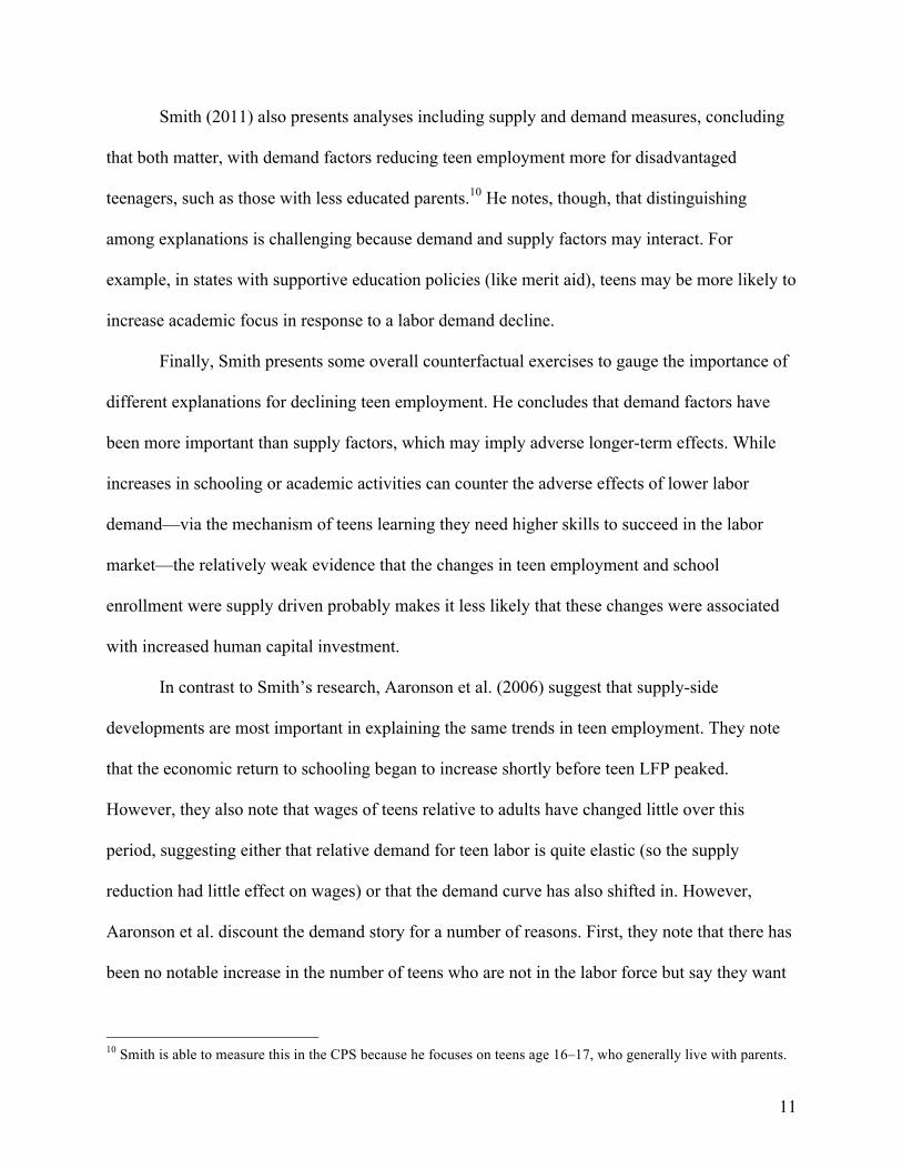
Smith (2011) also presents analyses including supply and demand measures, concluding

that both matter, with demand factors reducing teen employment more for disadvantaged

teenagers, such as those with less educated parents.10 He notes, though, that distinguishing

among explanations is challenging because demand and supply factors may interact. For

example, in states with supportive education policies (like merit aid), teens may be more likely to

increase academic focus in response to a labor demand decline.

Finally, Smith presents some overall counterfactual exercises to gauge the importance of

different explanations for declining teen employment. He concludes that demand factors have

been more important than supply factors, which may imply adverse longer-term effects. While

increases in schooling or academic activities can counter the adverse effects of lower labor

demand—via the mechanism of teens learning they need higher skills to succeed in the labor

market—the relatively weak evidence that the changes in teen employment and school

enrollment were supply driven probably makes it less likely that these changes were associated

with increased human capital investment.

In contrast to Smith’s research, Aaronson et al. (2006) suggest that supply-side

developments are most important in explaining the same trends in teen employment. They note

that the economic return to schooling began to increase shortly before teen LFP peaked.

However, they also note that wages of teens relative to adults have changed little over this

period, suggesting either that relative demand for teen labor is quite elastic (so the supply

reduction had little effect on wages) or that the demand curve has also shifted in. However,

Aaronson et al. discount the demand story for a number of reasons. First, they note that there has

been no notable increase in the number of teens who are not in the labor force but say they want

10 Smith is able to measure this in the CPS because he focuses on teens age 16–17, who generally live with parents.

12

a job, and indeed, as noted above, the long-term trend is toward a decline in the fraction of teens

who are not in the labor force but want a job. Second, they suggest that there has been relative

employment growth in the industries that typically hire teens. Third, relative teen wages have not

fallen—although of course higher minimum wages may have played a role in this.11

Curiously, the role of minimum wages has been largely ignored in this context, despite

the extensive literature on the effects of minimum wages on teenage employment (although the

conclusion is contested)12 and the much smaller body of literature on the effects of minimum

wages on schooling (discussed below). Mixon and Stephenson (2016) present results suggesting

that changes in the minimum wage explain the decline in teen summer employment. But their

analysis is based on aggregate time-series data and hence should not be viewed as convincing.

Perhaps the biggest gap the present paper fills is in providing a comprehensive analysis of the

role of minimum wages in changes in teen labor force (and schooling) behavior, and a

comparison of the effects of minimum wages to the other influences explored in the recent

literature on teen employment and school enrollment.

C. Longer-Run Implications of Changes in Teen Employment

Some research addresses the potential benefits of youth employment (partly through its

implications for schooling). Scott-Clayton and Minaya (2016) assess the impact of federal work-

study programs on academic and employment outcomes for university students. They apply a

novel form of propensity score matching to distinguish between the effects on students in two

11 Aaronson et al. do test the immigration hypothesis, but in a narrow way by redoing a Mariel-boatlift type analysis (Card 1990) for teen LFP. They also present a simple analysis suggesting that Hope scholarships partly account for the decline in teen LFP, but the effect is small. And they look at overall tuition effects and find qualitatively similar evidence. 12 For the most recent discussion of this evidence and the disputes, see Allegretto et al. (2017) and Neumark and Wascher (2017).

13

counterfactual situations: those who are induced into employment by the availability of work-

study and those who would have worked anyway (but not in a work-study job). Their conceptual

framework allows them to back out the effect of non-work-study employment for those who

otherwise would not have worked. This last group is the most relevant for the present study, and

for this group, the authors find negative effects of working while in school on short-run academic

achievement but a slightly higher probability of employment six years after program

participation. Their results suggest that a decrease in working while in school in favor of only

being in school could actually negatively impact future employment outcomes, despite

potentially positive effects on academic achievement.

Gelber et al. (2016) study experimental data (based on lotteries and IRS data) from the

New York City Summer Youth Employment Program, which offered summer jobs to youths age

14–21 during the years 2005–2008. The authors suggest that beneficial longer-run effects of

summer employment could include improving future employment outcomes and keeping youths

“out of trouble” and engaged in socially productive activities (as well as indirect effects via

supplemental income for low-income families). Although Gelber et al. found evidence of

increased earnings and employment in the year of program participation (without much

crowding-out of earnings from other employment), they found a modest decrease in earnings in

the three years after the program, and no effect on college enrollment.13

Smith (2011) motivates the concern with teen employment in terms of the economic

returns to early work. He notes that Ruhm (1997) and Light (2001) find some positive effects of

early work, while Hotz et al. (2002) wrestle more seriously with selection and find no effect or

13 However, they found reduced probabilities of incarceration (through 2013) and mortality (by 2014), although, as the authors acknowledge, the incarceration data are limited by excluding those age 18 or under.

14

perhaps even a negative effect.14 However, as Smith notes, this evidence is much older, being

from the 1979 National Longitudinal Survey of Youth (NLSY). Thus, he concludes, it is not

clear that less teen employment is necessarily bad for future human capital accumulation.

However, if immigration actually encourages more education in order to avoid competition with

immigrants or other low-skilled adults, then the human capital effect could be positive.

In work a bit closer to what we do in this paper, the working paper version of Smith (2012)

finds little evidence that lower teen employment rates are associated with higher earnings 10 years

later,15 suggesting that whatever lowered teen employment, it did not, on net, induce greater human

capital investment. This type of conclusion contrasts with some of the other work cited above,

suggesting that changes in teen behavior may have stemmed from factors such as increased

demands of schooling, merit-based scholarship programs to lower costs of college, and the like.

III. Descriptive Evidence on Changes in Teen Labor Market and School Enrollment Behavior

We begin by providing descriptive information on the evolution of teen LFP, employment, and

school enrollment, updating some of the evidence described in the previous section, and covering

the time period we analyze. Figure 1 plots LFP rates for those age 16–17, those age 18–19, and

older, broader age ranges from 1980 through 2016. These data and all the data used below,

except where otherwise noted, are from CPS March Supplement files.16 Figure 1 shows a clear

14 Smith notes that a negative or, at best, a weak positive effect may occur if working part-time during school detracts from academic activities (e.g., Rothstein 2007). 15 See Christopher L. Smith, “The Impact of Low-Skilled Immigration on the Youth Labor Market” (Finance and Economics Discussion Series, Federal Reserve Board, Washington, DC, December 2009), available at https://www .federalreserve.gov/pubs/feds/2010/201003/201003pap.pdf. 16 The CPS March Supplement data, and the American Community Survey (ACS) data discussed below, are made available by Integrated Public Use Microdata Series (IPUMS). The CPS Outgoing Rotation Group data discussed below are made available by the National Bureau of Economic Research (NBER). See https://cps.ipums.org/cps/ for the CPS March Supplement, https://usa.ipums.org/usa/ for the ACS, and http://www.nber.org/morg/annual/ for the CPS Outgoing Rotation Group data (all viewed September 10, 2017).

15

decline in participation of teenagers—both 16–17 years old and 18–19 years old—relative to

other age groups, beginning around 2000.

Figure 1. Labor Force Participation Rates (%) by Age Group, 1980–2016

Note: The gray shaded areas indicate recessions based on NBER recession dates.

Figure 2 provides more detail on labor force status, focusing only on those up to age 24.

There is clear evidence of increased unemployment rates for all groups beginning with the Great

Recession. But the figure also illustrates that, for teenagers, this was accompanied by a

(continuing) drop in LFP and hence also in the employment rate.

16

Figure 2. Labor Force Status (%) by Age, Subgroups of People Age 16–24, 1980–2016

Notes: The gray shaded areas indicate recessions based on NBER recession dates. “Unemp.” = unemployment. “Emp-pop ratio” = employment to population ratio.

Figure 3 examines the behavior underlying the changes in LFP (and employment). We

use information on employment and school activity of youths, relying on two independent

questions asked about school or college enrollment and information on employment status. The

four categories displayed in the figure—school only, work and school, work only, and idle—are

mutually exclusive and exhaustive. The left-hand panel, for those age 16–17, indicates no

changes in either the proportion only working or the proportion idle—and indeed both

proportions are very low for this age group. In contrast, there is a marked decline in the

proportion reporting that they are both in school and working, and a corresponding marked

increase in the proportion who report they are exclusively in school, beginning around 2000. The

17

evidence for those age 18–19, in the middle panel, is a bit more mixed. There is no change in

idleness. There are modest decreases in the proportions exclusively working or both working and

in school, and there is a more marked increase in the proportion in school only.

Figure 3. Employment and School Enrollment Status (%) by Age, Subgroups of People Age 16–24, 1986–2016

Notes: The gray shaded areas indicate recessions based on NBER recession dates.

Figure 4 gives a different perspective on these changes in the proportions exclusively in

school versus both in school and working, plotting the 1986–2016 changes by state, for people

age 16–17, 18–19, 16–19, and 20–24. This figure illustrates a number of points. First, for

teenagers, the proportion both working and in school declined for most states, and for people age

16–17 for all states but one (note where the points lie relative to zero on the horizontal axis).

18

Second, there is a fairly strongly negative relationship between the change in the proportion

working and in school and the change in the proportion exclusively in school; where the former

fell by more, the latter rose by more. And third, there is no such evidence for people age 20–24.

The points are generally to the right of zero on the horizontal axis, and there is no negative

correlation between the two types of changes.

Figure 4. Changes in Percentages in School Only vs. In School and Working, by State, Subgroups of People Age 16–24, 1986–2016

These results establish some key facts that set the stage for our subsequent analysis. First,

teen LFP and employment have fallen quite sharply since 2000. Second, these declines were not

accompanied by increases in idleness, but rather by increases in teens being exclusively in

19

school, rather than combining school and work. Third, these developments were rather unique to

teenagers. And fourth, the changes for teenagers were more pronounced for those age 16–17 than

for those age 18–19.

IV. Questions Raised by Developments in Teen LFP, Employment, and School Enrollment

These facts motivate the questions we investigate in this paper. First, we know that minimum

wages were increasing rather sharply in this period, with many states increasing their minimum

wage above the federal minimum wage, some quite substantially. Moreover, the average

minimum wage has risen sharply since around 2005 (see figure 5).17 The rising minimum wage

could have priced some teenagers out of the labor market. Given that the youngest workers have

the lowest skills, we would expect this pricing out to be more severe for teenagers (age 16–19)

than for young adults (age 20–24) and, among teenagers, to be more severe for those age 16–17.

There is ample evidence that higher minimum wages reduce employment of teenagers, although,

as noted above, this conclusion is contested by some.

However, it is unclear why higher minimum wages that adversely affect the employment

prospects of teenagers (in particular) would have primarily led to declines in employment among

those enrolled in school—increasing the proportion enrolled in school but not working and

reducing the proportion both in school and employed. Indeed, in past research on the effects of

minimum wages on teen employment and school enrollment, the findings differed. In particular,

Neumark and Wascher (1996, 2003) found that a higher minimum wage increased teen idleness

because of reduced employment among teenagers who were previously employed but not enrolled

17 The historical minimum wage data in figure 5 have been compiled from several sources. See http://www.socsci .uci.edu/~dneumark/datasets.html (viewed September 8, 2017).

20

in school, and it decreased school enrollment because some of those previously both enrolled and

employed left school and switched to being employed only (and increased their hours).18

Figure 5. Minimum Wages by State and Nationally (Population Weighted), 1979–2016

Notes: Values are shown in constant 2016 dollars. Population-weighted averages use the ratio of the earnings weights for people age 16–64 in each state to the total weights for all years of the sample. Pop-weighted avg. = population-weighted average. MW = minimum wage. Source: CPS Merged Outgoing Rotation Groups, 1979–2016.

The evidence concerning minimum wage effects on employment and schooling is dated,

and the empirical relationships may have changed. In general, minimum wages can either

increase or decrease schooling. They can decrease schooling if teens leave school to search for

18 As Neumark and Wascher (1996) note, the evidence is consistent with labor-labor substitution—with the higher-quality teens who are enrolled and working part-time switching to full-time work, thus displacing the lower-quality teens who had already dropped out of school.

21

work or if the induced wage compression at the bottom of the wage distribution reduces the

returns to schooling for those toward the bottom of the skill distribution. Or they can increase

schooling, as workers perceive a need to raise schooling to qualify for the higher-skilled jobs that

remain, as low-skilled jobs become less prevalent (Ehrenberg and Marcus 1982). One can

imagine that the various factors underlying this relationship have shifted in recent years. If this is

the case, higher minimum wages could have induced an increased focus on schooling that may

be reflected in the changes in teen school enrollment and employment documented above.

Alternatively, other changes that have coincided with more recent minimum wage

increases may underlie the shifts in teen employment and school enrollment since 2000. One

hypothesis is that increases in the returns to schooling, possibly complemented by the growth of

competitive scholarship programs (like the Hope program in Georgia), led teenagers to increase

their investment in schooling and hence, perhaps, to stop working while in school.19 Figure 6

provides evidence on the increase in the returns to schooling, defined as the education coefficient

in yearly Mincer regressions of log hourly wages on education, potential experience, a quadratic

in potential experience, and state fixed effects.20

19 Smith (2012) suggests that the decline in employment for those age 16–17 implies that the decline in teen employment generally cannot be owing to rising college attendance. However, the rising demands on time of high school students to generate this rising college attendance could explain the employment decline. 20 We constructed this series using the CPS Merged Outgoing Rotation Group (MORG) samples from 1979 to 2016. The MORG files offer the most consistent measure of hourly wages over the time period in question. For workers earning hourly wages, we use the reported hourly earnings, and for those reporting only weekly earnings, hourly wages are calculated as the ratio of weekly earnings to usual weekly hours worked. To construct the variable used in our analysis, we estimate returns to schooling by state and year. For figure 6, we estimate the returns to schooling by year (clustered at the state level). The regressions estimating the returns to schooling are run on individual-level data and weighted using the MORG individual earnings weights.

22

Figure 6. Increases in the Returns to Schooling, Ages 25–40, 1980–2016

Note: Plotted coefficients are from yearly Mincer regressions of log hourly wages on years of schooling, potential experience, a quadratic in potential experience, and state fixed effects, using individual-level data. Regressions are weighted using the MORG individual earnings weights. Grey area represents a 95 percent confidence interval. Source: CPS Merged Outgoing Rotation Groups 1979–2016.

The returns to schooling series in figure 6 is constructed for those age 25–40, the idea

being that teens may learn something about the returns to their investments in schooling by

observing earnings differentials associated with schooling among those somewhat older than

they. The increase in the returns to schooling is long standing. However, it was much sharper

before 2000, before stagnating and then rising more slowly after approximately 2005. Although

figure 6 provides no clear signal that we should have expected teens to increase their focus on

23

schooling and to reduce their work, beginning in 2000, the longer-term changes in behavior by

the end of the sample period could reflect responses to increases in the returns to schooling.21

A third hypothesis is that growth in the number of low-skilled immigrants has reduced

teen employment opportunities. The growth in the employed, Spanish-speaking immigrant share

(relative to the working-age native population) is depicted in figure 7. We measure this share

based on American Community Survey (ACS) data (which currently go only through 2015) and

on earlier Census data in order to increase the number of observations on immigrants, which is

especially important for smaller states.22 As with minimum wages, the most natural expectation

might be that an increase in immigration would reduce job opportunities for teenagers, thus

reducing employment. But it could also have increased the focus on schooling as teens invest

more in skills in order to qualify for higher-skilled jobs. That said, nothing dramatic changed in

2000 with regard to immigration inflows.23

21 There is, of course, a great deal of literature on potential biases in OLS estimates of returns to schooling, from factors such as omitted-ability bias and endogenous schooling choices (see, e.g., Card 1999). However, there is little, if any, evidence that sources of bias have changed over time so as to generate spurious evidence of increases in the returns to schooling (e.g., Blackburn and Neumark 1993), and it is common to describe the evolution of the returns to schooling in the United States without reference to such biases (e.g., Autor et al. 2008). Moreover, the mechanism we have in mind is what young people believe about the economic returns to schooling when they are making their schooling decisions, and they may well not “correct” for bias from omitted ability or other sources. 22 We use annual Census data through 1990 and ACS data beginning in 2000. Since the Census data are decadal, we linearly interpolate to fill in individual years not covered by the Census. Moreover, there is a discrete jump in the ACS data in the immigrant share (relative to the Census), apparent even in 2000 when the datasets overlap. We therefore adjust the ACS data downward by multiplying the data for 2001 onward by the ratio of the 2000 measure in the Census data to the 2000 measure in the ACS data, by state. 23 This is not the full set of potential explanations. Supplements to the federal Earned Income Tax Credit (EITC) in many states have brought more single mothers into the labor market, potentially displacing teenagers in much the same way as the inflow of immigrants. Neumark and Wascher (2011) show that these effects arise most strongly from interactions between minimum wages and the EITC; we leave addressing the potential effects of policy interactions (and interactions between policy and the other factors we consider) to future work. Smith (2011) also conjectured that some forms of technological change may have displaced medium-skilled adults into jobs where they are more likely to compete with teens (and younger adults); however, we have no data that address this hypothesis directly.

24

Figure 7. Increases in the Spanish-Speaking Immigrant Share Relative to Native Working-Age Population, 1986–2015

Note: Immigrants are defined as individuals having been born outside the United States to non-US citizens. The group of immigrants is restricted to those currently employed and from Spanish-speaking countries. The share is relative to the total working-age population of native-born Americans. Pop-weighted avg. = population-weighted average. Source: Census and ACS data, 1986–2015.

Of course, the shift of teens from being simultaneously employed and enrolled to being

exclusively enrolled in school may not entail any increased focus on schooling or investment in

skills. Instead, this change may simply reflect diminished job opportunities or increased

consumption of leisure. But for whatever reason, this is happening for students who would

otherwise have been employed as well as enrolled in school, so that they switch to enrolled only.

If this is a better characterization of the changes in teen employment and enrollment behavior,

then the only change in human capital investment by teenagers may have been a decline,

25

stemming from less accumulation of labor market experience—whether due to higher minimum

wages or immigration.

These considerations lead to two key questions: First, what explains the observed changes

in employment and school enrollment of teenagers? What were the roles of minimum wages,

immigration, and increases in the returns to schooling, and which of these was most important?

Second, what are the implications for human capital investment on the part of teenagers? If

teenagers are simply working less and not increasing their schooling investments, they may end

up with less human capital. In contrast, if the shift toward being exclusively enrolled in school

reflects greater investment in schooling, they may end up with more human capital.

V. Evidence on Sources of Changes in Teen Employment and Enrollment

We first estimate a grouped data version of a multinomial logit model for the share of teens in each

of the four mutually exclusive and exhaustive categories—not in school and not employed (NSNE

or idle), employed and not in school (ENS), in school and employed (SE), and in school and not

employed (SNE). We group the data by state and year, estimating the model for the logs odds

ratios for three of the four outcomes and using seemingly unrelated regressions (SURs), and then

computing and reporting the marginal effects for each of the four outcomes.24 Table 1 (page 51)

24 In this model, teens (indexed by i) make a discrete choice among J schooling and employment alternatives (indexed by j) according to a random utility function, !"# = %"&# + ("#, which represents the value of each alternative to the individual. %" denotes a set of individual-specific variables, and ("# is a random error component assumed to follow a Type I extreme value distribution. Teens will choose the alternative with the highest utility, in which case (given the distributional assumption) the probability of choosing any one alternative can be expressed as follows:

)"# =*+,(/0

123)

*+,(/0123)

5367

.

We use data aggregated to the state and age group level, so we add indices for state (s) and year (t), and we drop the i index. In the grouped data version of our model, we define the base category as in school and employed (SE) and use the log odds ratios of each observed probability as the dependent variable in the following system of equations:

26

reports estimates of models for teens age 16–17, table 2 (page 52) for those age 18–19, and table 3

(page 53) for those age 16–19, all for the period 1986–2015.25

The first four columns of table 1 mimic the standard minimum wage employment

specification, albeit for the different schooling and employment outcomes. We include the log of

the higher of the state or federal minimum wage (CPI-adjusted to constant dollars),26 the prime-

age male unemployment rate as a cyclical control, the population share of the age group studied

(here, teens age 16–17) as a supply or cohort-size control. We also add the black and Hispanic

shares in the age group, year, and state, and the share with at most a high school degree among

the working-age population in the state and year (the estimated coefficients of these last three

controls are not reported).27 All of these control variables are calculated using CPS March

Supplement data. The models also include state and year fixed effects. Regressions are weighted

using CPS sample weights and clustered at the state level.

log()#89 ):;89 ) = &<=>89 + &?@ABC89 + &DE==89 + &F!@89 + &GHIH89 + &J%89 + K9 + K8 + (#89.

=>89denotes the log of the higher of the contemporaneous state or federal minimum wage. @ABC89 denotes the returns to schooling observed by teens for their older peers, age 25–40. E==89 is the share of employed immigrants relative to the native working-age population. !@89 is the state’s unemployment rate among prime-age men, HIH89 is the teenage group’s share in the population, and %89 includes the shares of black and Hispanic teens within the age group as well as the share of high school graduates among the working-age population within the state.

This is the same method used in Neumark and Wascher (1995), and it was discussed in McFadden (1973). An alternative is to use the microdata and estimate a multinomial logit model. We show in appendix table A2 (page 59) that the results are very similar (the comparison is to table 1, discussed below). One advantage of the grouped data approach is that it is easier to use an instrument for the immigration share variable. 25 The first year in which the schooling variable is available in the CPS March Supplement files is 1986, and the ACS currently runs through 2015, limiting the observed time frame for regression results displayed in tables 1–3 to 1986–2015. 26 Since our models include year fixed effects, the year to which the minimum wage is deflated is immaterial. 27 Appendix table A1 (page 58) shows that the demographic composition of teens changed over our sample period, with a decline in the white share and an increase in the Hispanic share. We would expect this demographic shift to have some influence on teen employment rates, since white teens are more likely to work than Hispanic teens (as indicated by the representation of each group among working and nonworking teens). Indeed, in unreported results (available upon request), we show that teen employment would have been somewhat higher at the end of the sample period absent these demographic shifts. However, our interest is in the effects of policy and other economic factors on teen employment, conditional on workforce characteristics. Moreover, demographic composition obviously cannot account for much of the differences in changes in employment and school enrollment for those age 16–17 versus those age 18–19. Indeed, we have confirmed that the effect of this changing demographic composition is similar for these two subgroups of teenagers.

27

The estimates in columns 1–4, which include the minimum wage variable but not

variables capturing changes in the returns to schooling or immigration, give a clear indication

that higher minimum wages are associated with a lower share of those age 16–17 in school and

employed (SE) and a higher share in school and not employed (SNE), all corresponding to the

changes in teen behavior documented above. The point estimates, which are statistically

significant, imply that a 20 percent increase in the minimum wage lowers the SE share by about

0.022 and raises the SNE share by about 0.025. These changes are quite large relative to the

baseline shares (0.23 for SE and 0.72 for SNE).

Next, to ask whether changes in the returns to schooling can account for the changes in

teen employment and school enrollment (and perhaps the minimum wage effects suggested by

the estimates in columns 1–4), we add state-by-year estimates of the returns to schooling for

adults age 25–40 (the age group covered in figure 6).28 If increases in the return to schooling

over time are driving an increased focus on schooling for teens, we would expect positive effects

on statuses involving schooling (SE and SNE) and negative effects on statuses involving non-

enrollment (NSNE and ENS).

Alternatively, if the effects are concentrated among those in school, we might expect

more teens to be in school exclusively (a positive effect on SNE) and fewer teens to be employed

while in school (a negative effect on SE). As columns 5–8 show, the point estimates are

consistent with the latter, as there is a positive estimate on the probability of being in school and

not employed (SNE)—although the estimate is not statistically significant—and a negative effect

on the probability of being in school and employed simultaneously (SE)—statistically significant

28 Results were similar when we varied the age range used to estimate the returns to schooling over time, using adults age 20–35 and, alternatively, those age 25–54.

28

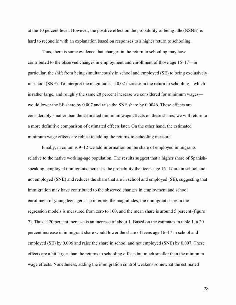
at the 10 percent level. However, the positive effect on the probability of being idle (NSNE) is

hard to reconcile with an explanation based on responses to a higher return to schooling.

Thus, there is some evidence that changes in the return to schooling may have

contributed to the observed changes in employment and enrollment of those age 16–17—in

particular, the shift from being simultaneously in school and employed (SE) to being exclusively

in school (SNE). To interpret the magnitudes, a 0.02 increase in the return to schooling—which

is rather large, and roughly the same 20 percent increase we considered for minimum wages—

would lower the SE share by 0.007 and raise the SNE share by 0.0046. These effects are

considerably smaller than the estimated minimum wage effects on these shares; we will return to

a more definitive comparison of estimated effects later. On the other hand, the estimated

minimum wage effects are robust to adding the returns-to-schooling measure.

Finally, in columns 9–12 we add information on the share of employed immigrants

relative to the native working-age population. The results suggest that a higher share of Spanish-

speaking, employed immigrants increases the probability that teens age 16–17 are in school and

not employed (SNE) and reduces the share that are in school and employed (SE), suggesting that

immigration may have contributed to the observed changes in employment and school

enrollment of young teenagers. To interpret the magnitudes, the immigrant share in the

regression models is measured from zero to 100, and the mean share is around 5 percent (figure

7). Thus, a 20 percent increase is an increase of about 1. Based on the estimates in table 1, a 20

percent increase in immigrant share would lower the share of teens age 16–17 in school and

employed (SE) by 0.006 and raise the share in school and not employed (SNE) by 0.007. These

effects are a bit larger than the returns to schooling effects but much smaller than the minimum

wage effects. Nonetheless, adding the immigration control weakens somewhat the estimated

29

minimum wage effects, and the minimum wage effect on the probability of being in school and

employed (SE) declines by about 20 percent and becomes statistically insignificant.

Because the observed immigrant share could be endogenously related to labor market

conditions that also drive teen behavior, we estimate the model using a shift-share instrument for

Spanish-speaking immigrants. We begin by taking the sum of Spanish-speaking, employed

immigrants in each state in the base year 1970, and we then multiply it by the yearly growth rate

of Spanish-speaking immigrants of working age in all states, excluding the given state for 1986–

2015. Finally, we divide it by the native working-age population in the given year. This is a

similar strategy to that used by Smith (2012) and in earlier work by Altonji and Card (1991) and

Card (2001). We construct this variable using the data described earlier.29

The validity of the instrument relies on two conditions. The first, which is an assumption,

is that the predicted share of Spanish-speaking employed immigrants in any given state

influences the employment and schooling decisions of teens in that state only through its effect

on the actual share of immigrants to natives (the exclusion restriction). This assumption could be

violated if, for example, in the initial period of 1970, some states were already in the midst of a

long-term economic shock that attracted Spanish-speaking immigrants and affected both base-

period and current labor market outcomes. Because the contemporaneous major immigration

waves of Spanish speakers did not pick up until well after 1970 (Bean and Tienda 1987), we

chose a very early base period such that this exclusion restriction can be expected to hold.30

Moreover, the instrument will not be biased by the relationship between immigration and time-

varying economic conditions in the state in later periods because the growth rate of the

29 We also ran specifications with instruments for other immigrant origin groups and for all immigrants regardless of origin, but we include only the results for the Spanish-speaking group because it was the only immigrant group for which we find a very strong first-stage regression. 30 Because our model is exactly identified, there is no formal test for exogeneity of the instrument.

30

immigrant share is calculated according to national growth rates, excluding the growth rate of the

given state.

The second condition for a valid instrument is that the predicted share of Spanish-

speaking immigrant workers has a strong correlation with the actual share. We test this rank

condition and confirm that the instrument is highly relevant, demonstrated by a first stage F-

statistic above 10 and often above 20. As reported in appendix table A3 (page 60), the results are

qualitatively similar when we use an instrument for immigration exposure or include the share of

employed Spanish-speaking immigrants to natives directly (as in table 3). Hence, going forward

we report results without instrumenting.31

The second-to-last row of table 1 provides a summary measure for employment effects,

reporting the estimated effect on the probability of employment without regard to enrollment

status; this is the sum of the effects on the ENS (employed, not in school) and SE (in school and

employed) cells. In all three specifications, the estimated employment effect is negative. The

implied elasticity is about −0.1, and it does diminish slightly as the returns-to-schooling and

immigration controls are added (becoming significant only at the 10 percent level).32

Thus, overall, the results for teenagers age 16–17 lead to two conclusions. First, higher

minimum wages partially explain the declining employment of teenagers and also help explain

the compositional shift underlying this decline (the switch from SE to SNE). Second, there is

some evidence that the other hypothesized factors—increases in the return to schooling and

competition from immigrants—also play a role. The evidence is statistically stronger with regard

31 The same holds for whether we instrument for the immigrant share in our longer-term analysis in section IV. 32 To translate this estimate into an elasticity to compare with standard results in the literature, a 10 percent increase in the minimum wage would then reduce the share of employed teens age 16–17 by about 0.01. This is about a 4 percent decline in the employment rate (which is 0.246, as shown in the “Probability of outcome” row). The implied elasticity is around −0.4, which is larger than the elasticity usually estimated for teens age 16–19.

31

to immigration, but the estimated effects of minimum wages are considerably larger than the

effects of either of these other two influences.

Tables 2 and 3 report similar estimates for teens age 18–19 and for teens age 16–19. The

basic conclusion from these two tables, in comparison to table 1, is that most of the effects for

those age 18–19 are weaker. In table 2 (page 52), the specifications without the immigration

control point to weaker minimum wage effects. Only the estimated (positive) effect on the

probability of being in school and not employed (SNE) is significant, and the overall

employment effect in the second-to-last row is negative but smaller and not statistically

significant. And in the specification in columns 9–12 including the immigration controls, none of

the estimated minimum wage effects are statistically significant. The estimated effects of

changes in the returns to schooling are smaller and statistically insignificant. And only the

estimated effect of the immigration share on the probability of being in school and not employed

(SNE) is statistically significant; this estimated coefficient is actually larger than the

corresponding estimate in table 1 and on a smaller base share (0.403 vs. 0.716).

In table 3 (page 53), combining all teenagers age 16–19, we get rough averages of the

effects from the previous two tables. In the full specification in columns 9–12, only the effects of

immigration are statistically significant, while the minimum wage effects on overall employment

(and the probability of being SNE) are significant before the immigration control is added.

Recall, though, that the changes in teen employment and school enrollment that we

documented earlier were more pronounced for those age 16–17. The estimates in tables 1–3

suggest that the minimum wage effects have the largest influence in explaining the changes in

labor market behavior of those age 16–17 that we have documented—including the overall

32

decline in their employment.33 However, there is also some evidence that the other factors matter

in the expected directions.

To provide clearer evidence on the magnitudes of these effects, we turn to simple

simulations that calculate the implied effects of changes in the minimum wage, returns to

schooling, and the immigration share from 2000 (when the changes in teen employment and

school enrollment emerged) to 2015. In figure 8, we focus on the implied effects of changes in

minimum wages on employment and school enrollment of teens age 16–17. The solid lines are

the actual observed series. The dashed lines, beginning in 2000, simply add the difference

implied by the estimated minimum wage (marginal) effects in columns 9–12 of table 1,

multiplied by the difference between the real minimum wage implied by holding the minimum

wage fixed at its 1999 nominal value and the actual real minimum wage (in both cases using the

national weighted average). That is, we show what would have happened, ceteris paribus, if the

minimum wage had not changed. We use 2000 as the starting point for the simulation because

that is roughly the year when the decline in teen employment began.

33 Indeed, the evidence on minimum wage employment effects for teenagers indicates a negative effect—and a much larger point estimate—only for those age 16–17. This evidence is interesting in light of critiques of standard panel data estimators (like the one used here) by Allegretto et al. (2011). Their assertion is that minimum wage increases are correlated with negative shocks to low-skilled labor markets that generate spurious evidence of job loss from higher minimum wages. This assertion has been disputed (Neumark et al. 2017; Neumark and Wascher 2017), and evidence from other approaches that would capture the influence of such shocks actually leads to stronger evidence of disemployment effects (e.g., Baskaya and Rubinstein 2015; Clemens and Wither 2016; and Liu et al. 2016). The new evidence presented here—that disemployment effects appear for teens age 16–17 but not for those age 18–19—further undermines the idea that such shocks generate spurious evidence of disemployment effects of minimum wages. Thus, this evidence should be immune to the Allegretto et al. criticism—unless, for some reason, minimum wage variation is correlated with shocks to the labor market for teens age 16–17 but not for those age 18–19.

33

Figure 8. Effects of Minimum Wage Changes on Employment and School Enrollment Status of Teens Age 16–17: Actual before 2000 and Simulated since 2000

Note: Observed shares of teens idle (NSNE), employed but not in school (ENS), in school and employed (SE), and in school but not employed (SNE), compared to the prediction if minimum wages had remained unchanged since 1999. Based on the grouped multinomial logit estimates with the complete set of control variables in table 1.

The panels in figure 8 point to rather large implied effects on the shares for which we

tended to find significant effects of minimum wages: SE (in school and employed) and SNE (in

school and not employed). (The effects on the ENS share [employed and not in school] look

large, but the vertical scale is much smaller.) Based on this simple simulation, the change in

minimum wages seems to account for about 21 percent of the decline (from 2000) in the SE

share and about 28 percent of the increase in the SNE share. As figure 9 shows, minimum wage

changes account for smaller percentages of the changes in behavior of teens age 16–19,

34

reflecting the smaller regression estimates for this broader teen group because of the weaker

relationships for those age 18–19.

Figure 9. Effects of Minimum Wage Changes on Employment and School Enrollment Status for Teens Age 16–19: Actual before 2000 and Simulated since 2000

Note: Observed shares of teens idle (NSNE), employed but not in school (ENS), in school and employed (SE), and in school but not employed (SNE), compared to the prediction if minimum wages had remained unchanged since 1999. Based on the grouped multinomial logit estimates with the complete set of control variables in table 3.

Figures 10 and 11 show similar simulation results for the changes in the returns to

schooling. In these figures, the effect of holding the returns to schooling unchanged beginning in

2000 barely results in visually detectable changes in the shares in the different enrollment and

employment categories. This is a reflection of two factors. First, as noted above, the estimated

effects of the returns to schooling are smaller than the estimated effects of minimum wages.

35

Second, as we saw in figure 6, the increase in the returns to schooling has been rather muted

since 2000, and most of the run-up occurred earlier.34

Figure 10. Effects of Returns to Schooling Changes on Employment and School Enrollment Status of Teens Age 16–17: Actual before 2000 and Simulated since 2000

Note: Observed shares of teens idle (NSNE), employed but not in school (ENS), in school and employed (SE), and in school but not employed (SNE), compared to the prediction if returns to schooling had remained unchanged since 1999. Based on the grouped multinomial logit estimates with the complete set of control variables in table 1.

34 A more complicated possibility is that teenagers learned slowly of the increase in the returns to schooling, and after 2000 they were responding to earlier changes.

36

Figure 11. Effects of Returns to Schooling Changes on Employment and School Enrollment Status of Teens Age 16–19: Actual before 2000 and Simulated since 2000

Note: Observed shares of teens idle (NSNE), employed but not in school (ENS), in school and employed (SE), and in school but not employed (SNE), compared to the prediction if returns to schooling had remained unchanged since 1999. Based on the grouped multinomial logit estimates with the complete set of control variables in table 3.

Figures 12 and 13 show similar simulation results for the changes in the immigrant share.

In this case, the effects on the shares in school and employed (SE) and in school and not

employed (SNE) are larger and in the same direction as the effects of minimum wages. But the

effects are much smaller than those in figures 8 and 9 for minimum wages—again because of

smaller estimated effects in the models and because the immigrant share did not change as

sharply after 2000 (compare figures 5 and 7).

37

Figure 12. Effects of Spanish-Speaking Immigrant Share Changes on Employment and School Enrollment Status of Teens Age 16–17: Actual before 2000 and Simulated since 2000

Note: Observed shares of teens idle (NSNE), employed but not in school (ENS), in school and employed (SE), and in school but not employed (SNE) compared to the prediction if immigration from Spanish-speaking countries had remained unchanged since 1999. Based on the grouped multinomial logit estimates with the complete set of control variables in table 1.

38

Figure 13. Effects of Spanish-Speaking Immigrant Share Changes on Employment and School Enrollment Status of Teens Age 16–19: Actual before 2000 and Simulated since 2000

Note: Observed shares of teens idle (NSNE), employed but not in school (ENS), in school and employed (SE), and in school but not employed (SNE) compared to the prediction if immigration from Spanish-speaking countries had remained unchanged since 1999. Based on the grouped multinomial logit estimates with the complete set of control variables in table 3.

Finally, figures 14 and 15 combine the results to obtain the simulated effects on

employment overall (the shares in school and employed [SE] plus employed and not in school

[ENS]). Figure 14 shows that, for those age 16–17, the minimum wage effect is predominant.

For teens age 16–19, figure 15 shows that the minimum wage and immigration effects are closer,

although the former are a bit larger.

39

Figure 14. Effects of Minimum Wage, Returns to Schooling, and Spanish-Speaking Immigrant Share Changes on Employment (SE + ENS) Status of Teens Age 16–17: Actual before 2000 and Simulated since 2000

Note: Notes to figures 8–13 apply, but the outcome is observed shares of teens employed but not in school (ENS) plus in school and employed (SE). Based on estimates in table 1.

40

Figure 15. Effects of Minimum Wage, Returns to Schooling, and Spanish-Speaking Immigrant Share Changes on Employment (SE + ENS) Status of Teens Age 16–19: Actual before 2000 and Simulated since 2000

Note: Notes to figures 8–13 apply, but the outcome is observed shares of teens employed but not in school (ENS) plus in school and employed (SE). Based on estimates in table 3.

The overall conclusion, therefore, is that all three factors—the increase in minimum

wages, rising returns to schooling, and a higher immigrant share—help explain the decline in

teen employment and more generally changes in teen employment and school enrollment. But

the predominant factor underlying changes in teen employment and enrollment that began in

2000—in particular, for those age 16–17—is the higher minimum wage. Changes in

immigration played a more limited role, and changes in returns to schooling appear to have had

a negligible influence.

41

VI. Implications of Minimum Wage Effects on Teenagers for Human Capital Investment

Had we found that increases in the returns to schooling are the predominant explanation for the

shift of teenagers from combining work and schooling to being exclusively enrolled in school, it

would be quite natural to presume that the changes reflect an increased focus on schooling and

hence greater human capital investment. However, minimum wages appear to be the

predominant driver of this shift (among those drivers we have studied), and immigration the next

most important. Since both of these influences are likely associated with fewer opportunities to

accumulate experience in the labor market but could also spur teenagers to invest more in human

capital in order to qualify for higher-skilled jobs, the potential effects on human capital

investment are ambiguous.

One potentially promising finding with regard to human capital investment is that the

evidence on the effects of minimum wages on teens’ schooling and employment choices is more

consistent with the minimum wage leading to higher human capital investment among teenagers

than was earlier evident. Specifically, the evidence on the effects of minimum wages on

employment and school enrollment, in tables 1–3, is different from that found by Neumark and

Wascher (1996, 2003). Using data for 1980–1998, Neumark and Wascher (2003) find evidence

that a higher minimum wage increased idleness (NSNE) and increased the likelihood of being

employed and not enrolled (ENS). These results aligned with evidence from microdata on

schooling and employment transitions (Neumark and Wascher 1996) that a higher minimum

wage led some students to leave school for jobs, displacing from employment those who had

already dropped out and were working—likely a form of labor-labor substitution from less-

productive to more-productive teenagers.

42

In contrast, as seen in table 3, there is no evidence of an increase in idleness, and the

effect of the minimum wage is more consistent with employed students leaving employment.

This latter kind of change could be consistent with a positive human capital response to a higher

minimum wage—if the teens in school and no longer employed were devoting more effort to

schooling, which is consistent with some of the other types of evidence discussed in section II. In

contrast, the earlier evidence (less schooling, increased idleness) is more consistent with a

negative human capital response to a higher minimum wage, especially because the net effect on

employment was not positive. Nonetheless, forgone work experience while in school could have

adverse effects on human capital accumulation.

To assess this question, we use an approach first used in Neumark and Nizalova (2007).

They estimated the effects of exposure to a higher minimum wage as a teenager on wages and

earnings of adults. Their focus was on the human capital costs of forgone labor market

experience stemming from disemployment effects of minimum wages for teenagers (and

possibly reduced training), but the evidence can also capture any effect of minimum wages on

raising wages or earnings in the longer term, including more schooling (or greater investment in

schooling for the same measured level of schooling).

We estimate the long-run impact of minimum wages—on those age 25–29 or 25–34—by

OLS, for the years 1985–2016, which is the longest observable time frame, given our included

variables.35 Following Neumark and Nizalova (2007), in order to avoid potential distortion from

35 We also look at subperiods. Our estimation equation is as follows:

L"89 = M + &<=>89<J<N + &?@ABC89<J<N + &DE==89

<J<N + &F!@89<J<N + &GHIH89<J<N + &J=>89?G?N + &O%89?G?N + KP

+K8 + K9 + ("89,

where i indexes the single-year age group of adults 25–29 years old in each state. Variables with the superscript 1619 are the “exposure” variables: average log minimum wage, returns to schooling, immigration, the prime-age male unemployment rate, and the population share of the given teenage group. =>"9

?G?N is the contemporaneous log minimum wage, and %"9?G?N captures the shares of black and Hispanic individuals in the age group. Single-year age

43

the Vietnam War draft, we wanted to include only cohorts that were 16 or younger in 1973, which

would make 1982 the first potential year in which we observe teen cohorts as adults of at least 25

years of age who were not affected by the draft. However, our explanatory variable for earlier

exposure to returns to schooling pushes the first year of observation for our analysis to 1985.36

Exposure to minimum wages as a teen is then calculated as the log of the average minimum wage

in effect when the individual was 16–19 years of age.37 This measurement of course assumes that

people lived as teenagers where they currently live when observed as adults; we have no way to

measure prior state residence in the CPS data. Our expectation is that misclassification of earlier

state of residence mutes any effects of exposure to minimum wages as a teenager. It is harder to

speculate about potential biases from endogenous migration, if that is an issue.

The models also include current demographic shares, the current minimum wage, and the

prime-age male unemployment rate to which one was exposed as a teenager in order to isolate

the effects of earlier minimum wages, as opposed to other current sources of low employment

opportunities. Finally, we also include the same returns-to-schooling and immigration measures

as above, both adjusted to reflect the time period when adult (25–29 and 25–34) cohorts were

teens (16–19). Including the teen exposure variables for minimum wages, returns to schooling,

and immigration provides us with the same “horse race” we conducted with respect to teen

dummies are denoted by KP, state fixed effects are denoted by K8, and K9 are year fixed effects. L"9 denotes, alternatively, log wages, log weekly earnings, and years of completed education. ("89 is an idiosyncratic error term. 36 The “returns to schooling” variable is constructed using MORG data, available from 1979 onward. The oldest teen (age 19) for whom we observe the returns to schooling in 1979 hits age 25 (our youngest “adult” age) in 1985. 37 One question we do not explore in this paper is the potential for heterogeneity in these effects by family income, race, etc. That is, there may be some groups for whom teen employment is falling because of greater investment in schooling, possibly leading to net positive effects on human capital accumulation, while for other groups the decline in teen employment is demand driven, with likely negative effects on human capital accumulation. It is plausible that the latter effect is stronger for minorities and other disadvantaged groups. Unfortunately, in the CPS data, we have no way of inferring family income at much earlier ages. Furthermore, sample sizes are too small to reliably study minority groups, as evidenced by the general lack of precise estimates for teenage minority groups in the standard literature on minimum wage and employment (e.g., Allegretto et al. 2011).

44

employment and school enrollment behavior. The difference here, however, is that we are trying

to estimate longer-term effects on human capital.

All outcome variables in the long-run regressions are constructed using the CPS Merged

Outgoing Rotation Group (MORG) data. Controls for the shares of black and Hispanic

individuals among the working-age population, the average population share at 16–19, and

exposure to the prime-age male unemployment rate at ages 16–19 are, as before, created in the

CPS March Supplement data and merged in by state and year.

Table 4 (page 54) reports results for adults age 25–29, and table 5 (page 55) for adults

age 25–34. In both tables, the estimates in columns 1 and 2 show that, for the entire 1985–2016

sample period, exposure to a higher minimum wage as a teenager is associated with lower wages

or earnings as an adult, and the estimates are statistically significant in both columns of both

tables. This is consistent with a higher minimum wage reducing human capital investment—

although this evidence does not let us parse out which type of investment is lower. Moreover,

although we cannot measure much human capital directly, we find no evidence of an effect on

completed years of schooling. On the other hand, we do find evidence that higher returns to

schooling at ages 16–19 are associated with higher weekly earnings and more schooling for both

adults age 25–29 and adults age 25–34.38 Earlier exposure to immigration also appears to induce

a small and statistically significant increase in years of completed education, but it does not have

a detectable impact on wages or earnings of adults.

Next, we split the sample into two subperiods. The first period roughly corresponds to the

sample period used by Neumark and Nizalova (2007). The estimate is in the same direction as

38 Recall that while the estimated coefficients seem larger, they should be applied to small changes in the variable—such as a 0.02 increase.

45

their results, pointing to lower earnings for adults age 25–29 from exposure to a higher minimum

wage as a teenager, although in our analysis the estimate is not statistically significant.39

The estimates for 2000–2016 are of more interest to the present paper, since they overlap

more with the period in which teen employment and school enrollment began to change the

most. The estimated wage and earnings effects are similar to those for the full period (in columns

1 and 2), although, in general, the evidence by subperiod is statistically weaker. A sharper

contrast is provided by the estimated effects on schooling of adults age 25–29 and 25–34, which

become positive.40 Although this subperiod estimate is not significant, this evidence is consistent

with higher minimum wages leading to greater human capital investment, via schooling, among

the teen cohorts after 2000 that shifted from simultaneous employment and school enrollment to

being exclusively enrolled in school in response to the minimum wage.

Nonetheless, it makes sense to interpret the overall effects on wages or earnings as

speaking more to overall effects on human capital, which can include the forgone employment

opportunities. Thus, qualitatively the evidence suggests that a higher minimum wage as a

teenager, on net, leads to lower human capital among adults. But the evidence is not very strong.

One could read the point estimates (e.g., 6.4 to 7.0 log points for wages and 15.6 to 19.5 log

points for weekly earnings) as rather large, and an insignificant effect (which we find for three

out of four cases) does not imply a zero effect. Alternatively, one can reach the stronger

conclusion, perhaps, that there is no evidence of net-positive human capital effects from higher

minimum wages.

39 Neumark and Nizalova did not look at adults age 30–34, in part because for these cohorts, in the earlier data, there is very little variation in minimum wages faced by teenagers. 40 As reported in appendix table A4 (page 61), the results across all of the specifications and samples in table 4 are robust when we estimate the model by 2SLS, instrumenting the possibly endogenous observed share of immigrant workers from Spanish-speaking countries relative to the native working-age population with the predicted share.

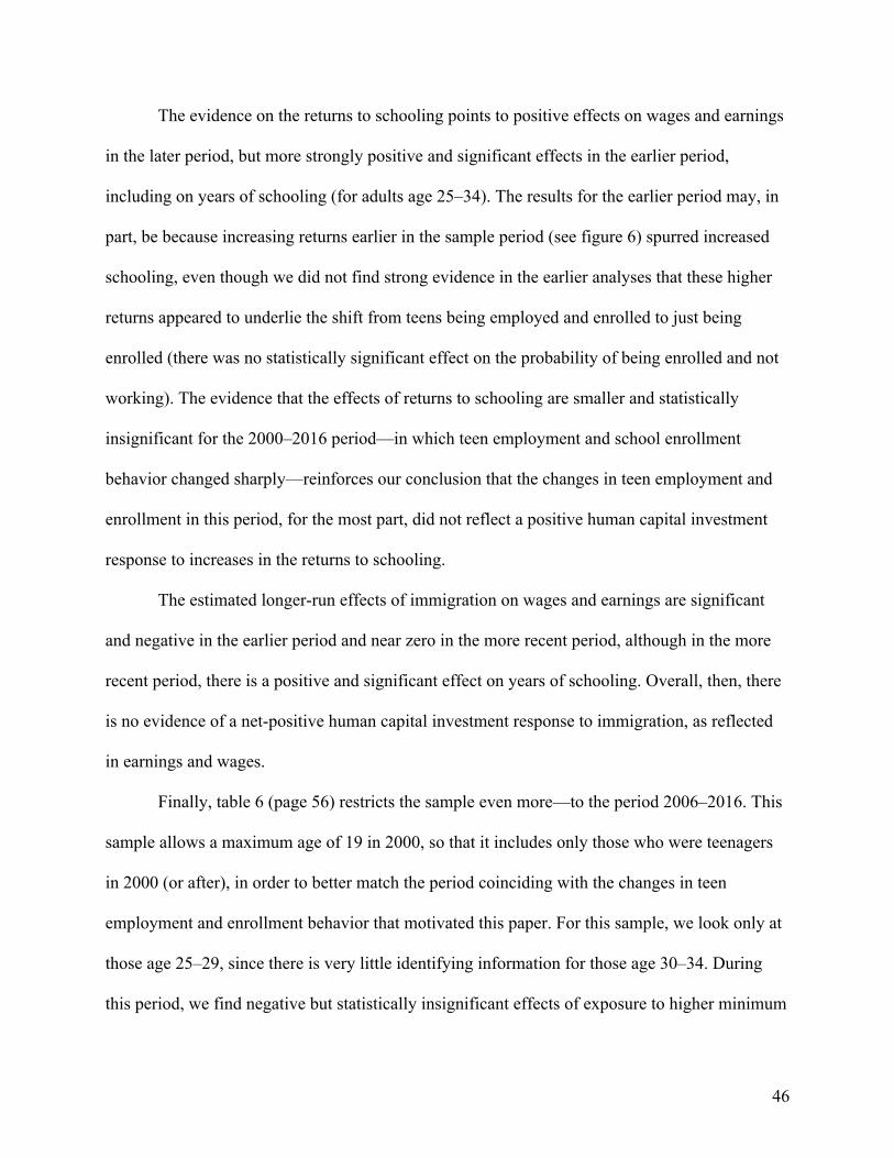
46

The evidence on the returns to schooling points to positive effects on wages and earnings

in the later period, but more strongly positive and significant effects in the earlier period,

including on years of schooling (for adults age 25–34). The results for the earlier period may, in

part, be because increasing returns earlier in the sample period (see figure 6) spurred increased

schooling, even though we did not find strong evidence in the earlier analyses that these higher

returns appeared to underlie the shift from teens being employed and enrolled to just being

enrolled (there was no statistically significant effect on the probability of being enrolled and not

working). The evidence that the effects of returns to schooling are smaller and statistically

insignificant for the 2000–2016 period—in which teen employment and school enrollment

behavior changed sharply—reinforces our conclusion that the changes in teen employment and

enrollment in this period, for the most part, did not reflect a positive human capital investment

response to increases in the returns to schooling.

The estimated longer-run effects of immigration on wages and earnings are significant

and negative in the earlier period and near zero in the more recent period, although in the more

recent period, there is a positive and significant effect on years of schooling. Overall, then, there

is no evidence of a net-positive human capital investment response to immigration, as reflected

in earnings and wages.

Finally, table 6 (page 56) restricts the sample even more—to the period 2006–2016. This

sample allows a maximum age of 19 in 2000, so that it includes only those who were teenagers

in 2000 (or after), in order to better match the period coinciding with the changes in teen

employment and enrollment behavior that motivated this paper. For this sample, we look only at

those age 25–29, since there is very little identifying information for those age 30–34. During

this period, we find negative but statistically insignificant effects of exposure to higher minimum

47

wages as a teen on wages and earnings; however, the weekly earnings effect is nearly significant

at the 10 percent level (p-value = 0.11). And the point estimate for years of schooling is negative.

There is no significant evidence of an effect of returns to schooling on either wages or earnings

and only an economically small but significant negative effect of immigration on log wages.

Thus, the evidence, if anything, says that teens exposed to higher minimum wages since

2000—the same teens who left combined employment and school enrollment for enrollment

only—had lower human capital investment. And while increases in the returns to schooling and

immigration may have also partly accounted for the changes in teen employment and

enrollment behavior since 2000, these increases do not appear to have resulted in higher human

capital investment.

VII. Conclusions

Our goal in this paper was twofold. First, we sought to understand the sources of the decline in

teen employment that began around 2000—in particular, the decline in employment among those

age 16–17—as well as, more generally, changes in teen employment and school enrollment

behavior. Second, we wanted to explore the implications of these changes for human capital,

given that the decline in employment consisted of fewer teens in school and employed, and more

teens in school exclusively, suggesting a greater focus on schooling. We have considered three

explanatory factors: (1) a rising minimum wage that could reduce employment opportunities for

teens and potentially also increase the value of investing in schooling; (2) rising returns to

schooling; and (3) increasing competition from immigrants that, like the minimum wage, could

reduce employment opportunities but also raise the returns to human capital investment.

48

With respect to the first question, we find some evidence of the expected effects of all

three explanatory factors on teen employment and school enrollment—and in particular for those

age 16–17. However, in terms of explaining changes in the behavior of teens age 16–17 since

2000, the role of the minimum wage is predominant. Increases in the returns to schooling appear

to have played almost no role, and immigrant competition a minor role. In contrast, our simulation

results suggest that minimum wages explain about a quarter of the shift, since 2000, from being

simultaneously employed and enrolled in school to being exclusively enrolled in school.

Turning to the second question, our examination of the longer-term effects of these three

factors uncovers no evidence that higher minimum wages, which underlie teens shifting from

combining work and schooling to being in school exclusively, led to greater human capital

investment. If anything, the evidence is in the other direction. Thus, it is more likely that the

principal effect of higher minimum wages in the 2000s, in terms of human capital, was to reduce

employment opportunities that could enhance labor market experience. Further, we find no

evidence of net-positive human capital effects of rising returns to schooling or increased

immigration in this period, even though these latter two factors—more so immigration—played

at least a minor role in the changes in teen employment and school enrollment.

Based on this evidence, then, it appears that the changes in teen labor market and schooling

behavior since 2000—stemming in part from adverse effects of minimum wages on employment

opportunities, and to a lesser extent from immigration—did not reflect greater human capital

investment that would raise future earnings. It is not clear that immigration delivered any other

short-term benefits to teens. In contrast, some teens surely benefited directly in the short run from

higher minimum wages. But there appear to have been either no effects or adverse effects on

longer-run earnings for those exposed to these higher minimum wages as teenagers.

49

References Aaronson, Daniel, Kyung-Hong Park, and Daniel Sullivan. 2006. “The Decline in Teen Labor

Force Participation.” Economic Perspectives 10:2–18. Aguiar, Mark, Mark Bils, Kerwin Kofi Charles, and Erik Hurst. 2017. “Leisure Luxuries and the

Labor Supply of Young Men.” NBER Working Paper No. 23552, National Bureau of Economic Research, Cambridge, MA.

Allegretto, Sylvia A., Arindrajit Dube, and Michael Reich. 2011. “Do Minimum Wages Really

Reduce Teen Employment? Accounting for Heterogeneity and Selectivity in State Panel Data.” Industrial Relations 50 (2): 205–40.

Allegretto, Sylvia A., Arindrajit Dube, Michael Reich, and Ben Zipperer. 2017. “Credible

Research Designs for Minimum Wage Studies: A Response to Neumark, Salas, and Wascher.” Industrial and Labor Relations Review 70 (3): 559–92.

Altonji, Joseph G., and David Card. 1991. “The Effects of Immigration on the Labor Market

Outcomes of Less-Skilled Natives.” In Immigration, Trade, and the Labor Market, edited by John M. Abowd and Richard B. Freeman. Chicago: University of Chicago Press.

Autor, David H., Lawrence F. Katz, and Melissa S. Kearney. 2008. “Trends in U.S. Wage

Inequality: Revising the Revisionists.” Review of Economics and Statistics 90 (2): 300–323.

Baskaya, Yusuf Soner, and Yona Rubinstein. 2015. “Using Federal Minimum Wages to Identify

the Impact of Minimum Wages on Employment and Earnings across the U.S. States.” Unpublished paper.

Bean, Frank D., and Marta Tienda. 1987. The Hispanic Population of the United States. New

York: Russell Sage Foundation. Bengali, Leila, Mary Daly, and Rob Valletta. 2013. “Will Labor Force Participation Bounce

Back?” FRBSF Economic Letter, No. 2013–14. Blackburn, McKinley L., and David Neumark. 1993. “Omitted-Ability Bias and the Increase in

the Return to Schooling.” Journal of Labor Economics 11 (3): 521–44. Card, David. 1990. “The Impact of the Mariel Boatlift on the Miami Labor Market.” Industrial

and Labor Relations Review 43 (2): 245–57. Card, David. 1999. “The Causal Effect of Education on Earnings.” In Handbook of Labor

Economics, Vol. 3, Part A, edited by Orley Ashenfelter and David Card, 1801–63. Amsterdam: Elsevier.

50

Card, David. 2001. “Immigrant Inflows, Native Outflows, and the Local Labor Market Impacts of Higher Immigration.” Journal of Labor Economics 19 (1): 22–64.

Clemens, Jeffrey, and Michael Wither. 2016. “The Minimum Wage and the Great Recession:

Evidence of Effects on the Employment and Income Trajectories of Low-Skilled Workers.” Unpublished paper.

Ehrenberg, Ronald G., and Alan J. Marcus. 1982. “Minimum Wages and Teenagers’ Enrollment-

Employment Outcomes: A Multinomial Logit Model.” Journal of Human Resources 17 (1): 39–58.

Gelber, Alexander, Adam Isen, and Judd B. Kessler. 2016. “The Effects of Youth Employment:

Evidence from New York City Lotteries.” Quarterly Journal of Economics 131 (1): 423–60.

Heckman, James J., and Paul A. LaFontaine. 2010. “The American High School Graduation

Rate: Trends and Levels.” Review of Economics and Statistics 92 (2): 244–62. Hotz, V. Joseph, Lixin Colin Xu, Marta Tienda, and Avner Ahituv. 2002. “Are There Returns to

the Wages of Young Men from Working While in School?” Review of Economics and Statistics 84 (2): 221–36.

Krueger, Alan B. 2015. “How Tight Is the Labor Market?” NBER Reporter No. 3. Light, Audrey. 2001. “In-School Work Experience and the Returns to Schooling.” Journal of

Labor Economics 19 (1): 65–93. Liu, Shanshan, Thomas J. Hyclak, and Krishna Regmi. 2016. “Impact of the Minimum Wage on

Youth Labor Markets.” Labour 30 (1): 18–37. McFadden, Daniel. 1973. “Conditional Logit Analysis of Qualitative Choice Behavior.” In

Frontiers of Econometrics, edited by Paul Zarembka, 105–42. New York: Academic Press.

Mixon, J. Wilson Jr., and E. Frank Stephenson. 2016. “Young and Out of Work: An Analysis of

Teenage Summer Employment, 1972–2012.” Cato Journal 36 (1): 89–99. Morisi, Teresa L. 2008. “Youth Enrollment and Employment during the School Year.” Monthly

Labor Review, February: 51–63. ———. 2010. “The Early 2000s: A Period of Declining Teen Summer Employment Rates.”

Monthly Labor Review, May: 23–35. Neumark, David, and Olena Nizalova. 2007. “Minimum Wage Effects in the Longer Run.”

Journal of Human Resources 42 (2): 435–52.

51

Neumark, David, J.M. Ian Salas, and William Wascher. 2017. “Reply to ‘Credible Research Designs for Minimum Wage Studies.’” Industrial and Labor Relations Review 70 (3): 593–609.

Neumark, David, and William Wascher. 1995. “Minimum Wage Effects on Employment and

School Enrollment.” Journal of Business and Economic Statistics 13 (2): 199–206. ———. 1996. “The Effects of Minimum Wages on Teenage Employment and Enrollment:

Estimates from Matched CPS Data.” Research in Labor Economics 15:25–64. ———. 2003. “Minimum Wages and Skill Acquisition: Another Look at Schooling Effects.”

Economics of Education Review 22 (1): 1–10. ———. 2011. “Does a Higher Minimum Wage Enhance the Effectiveness of the Earned Income

Tax Credit?” Industrial and Labor Relations Review 64 (4): 712–46. Porterfield, Shirley L., and Anne E. Winkler. 2007. “Teen Time Use and Parental Education:

Evidence from the CPS, MTF, and ATUS.” Monthly Labor Review, May: 37–56. Ross, Martha, and Nicole Prchal Svajlenka. 2015. “Worrying Declines in Teen and Young Adult

Employment.” Brookings Institution, December 16. Rothstein, Donna S. 2007. “High School Employment and Youths’ Academic Achievement.”

Journal of Human Resources 42 (1): 194–213. Ruhm, Christopher J. 1997. “Is High School Employment Consumption or Investment?” Journal

of Labor Economics 15 (4): 735–76. Scott-Clayton, Judith, and Veronica Minaya. 2016. “Should Student Employment Be

Subsidized? Conditional Counterfactuals and the Outcomes of Work-Study Participation.” Economics of Education Review 52 (June): 1–18.

Smith, Christopher L. 2011. “Polarization, Immigration, Education: What’s behind the Dramatic

Decline in Youth Employment?” Finance and Economics Discussion Series No. 2011-41, Federal Reserve Board, http://www.federalreserve.gov/pubs/feds/2011/201141/201141 pap.pdf.

———. 2012. “The Impact of Low-Skilled Immigration on the Youth Labor Market.” Journal of

Labor Economics 30 (1): 55–89. US Bureau of Labor Statistics. 2002. “Declining Teen Labor Force Participation.” Issues in

Labor Statistics, Summary 02-06.

52

Table 1. SUR Grouped Multinomial Model Estimates of Effects on Log-Odds Ratios of Different Employment and Enrollment Status, Teens Age 16–17, 1986–2015, Marginal Effects on Probability of Status

NSNE(1)

ENS(2)

SE(3)

SNE(4)

NSNE(5)

ENS(6)

SE(7)

SNE(8)

NSNE(9)

ENS(10)

SE(11)

SNE(12)

Independentvariable

LogMW −0.003(0.015)

−0.013(0.010)

−0.111***

(0.039)0.127***

(0.029)−0.007(0.015)

−0.013(0.009)

−0.100**

(0.040)0.120***

(0.029)−0.006(0.014)

−0.011(0.007)

−0.078(0.053)

0.095**

(0.041)

Returnstoschooling,25–40 … … … … 0.140**

(0.066)0.004(0.058)

−0.372*

(0.200)0.228(0.221)

0.145**

(0.066)0.004(0.057)

−0.381*

(0.200)0.232(0.220)

Immigrantshare(Spanish-speakingorigin) … … … … … … … … −0.0004

(0.0007)−0.0004(0.0006)

−0.006***

(0.002)0.007***

(0.002)Prime-agemaleunemploymentrate

0.005(0.050)

−0.099***

(0.034)−0.720***

(0.127)0.813***

(0.137)0.0004(0.049)

−0.099***

(0.034)−0.704***

(0.119)0.804***

(0.132)0.001(0.050)

−0.098***

(0.032)−0.684***

(0.125)0.785***

(0.131)

Populationshare 0.145(0.184)

−0.003(0.073)

−0.871**

(0.349)0.729*

(0.403)0.134

(0.108)−0.003(0.074)

−0.843**

(0.342)0.712*

(0.400)0.137(0.108)

−0.001(0.075)

−0.796**

(0.348)0.665(0.405)

Probabilityofoutcome 0.037 0.019 0.227 0.716 0.037 0.019 0.227 0.716 0.037 0.019 0.227 0.716CombinedMW −0.124*** −0.113*** −0.090* employmenteffect(ENS+SE) (0.033) (0.035) (0.048)

Observations 1,530 1,530 1,530 1,530 1,530 1,530 1,530 1,530 1,530 1,530 1,530 1,530Notes: SUR = seemingly unrelated regressions; NSNE = not in school and not employed; ENS = employed and not in school; SE = in school and employed; SNE = in school and not employed; MW = minimum wage. Estimates are based mainly on CPS March files. We implement a multinomial logit model by first calculating log odds ratios of each choice category by state and year in relation to the base category of SE. We then estimate the effect of the independent variables on the log odds ratios as a SUR system. The table displays the marginal effects. Each panel is estimated separately, incrementally including additional explanatory variables of interest. The left panel shows results excluding the ratio of Hispanic immigrant workers to the native working-age population as well as the “returns to schooling” (of adults age 25–40) variable. The middle panel adds the “returns to schooling” variable (supply control), and the right panel displays results for the full model. All regressions include state and year fixed effects, the nonblack Hispanic share and the black share in the given age group, and the share with at most a high school degree among the working-age population. The unemployment rate and population share variables are measured on a scale from 0 to 1 (i.e., proportions), and the returns to schooling are measured in log points (and in the data range from approximately 0.04 to 0.17). The Spanish-speaking immigrant share variable is measured on a scale of 0 to 100 (i.e., percentages). Observation numbers are the result of aggregating the data to state-by-year cells. ***, **, and * indicate that estimate is statistically significant from zero at the 1, 5, or 10 percent level, respectively. Standard errors are estimated clustering by state, and regressions are weighted using the sum of the individual CPS supplement weights.

53

Table 2. SUR Grouped Multinomial Model Estimates of Effects on Log-Odds Ratios of Different Employment and Enrollment Status, Teens Age 18–19, 1986–2015, Marginal Effects on Probability of Status

NSNE(1)

ENS(2)

SE(3)

SNE(4)

NSNE(5)

ENS(6)

SE(7)

SNE(8)

NSNE(9)

ENS(10)

SE(11)

SNE(12)

Independentvariable

LogMW −0.038(0.029)

−0.037**

(0.016)−0.009(0.031)

0.085***

(0.030)−0.038(0.028)

−0.029*

(0.017)−0.012(0.032)

0.079**

(0.035)−0.035(0.029)

−0.012(0.024)

−0.003(0.036)

0.050(0.045)

Returnstoschooling,25–40 … … … … −0.009(0.178)

−0.297(0.253)

0.114(0.179)

0.193(0.035)

−0.008(0.177)

−0.299(0.255)

0.127(0.177)

0.181(0.308)

Immigrantshare(Spanish-speakingorigin) … … … … … … … … −0.001

(0.001)−0.004**

(0.002)−0.003(0.001)

0.008***

(0.002)Prime-agemaleunemploymentrate

0.166(0.088)

−0.723***

(0.126)−0.255(0.139)

0.811***

(0.165)0.166(0.088)

−0.710***

(0.127)−0.259(0.136)

0.803***

(0.162)0.169*

(0.086)−0.697(0.132)

−0.253(0.139)

0.782***

(0.161)

Populationshare −0.492*

(0.287)0.071(0.285)

0.556(0.370)

−0.136(0.409)

−0.491*

(0.289)0.103(0.286)

0.544(0.373)

−0.156(0.403)

−0.484*

(0.293)0.152(0.284)

0.570(0.370)

−0.238(0.397)

Probabilityofoutcome 0.131 0.192 0.274 0.403 0.131 0.192 0.274 0.403 0.131 0.192 0.274 0.403CombinedMW −0.047 −0.041 −0.015 employmenteffect(ENS+SE) (0.035) (0.038) (0.052)

Observations 1,530 1,530 1,530 1,530 1,530 1,530 1,530 1,530 1,530 1,530 1,530 1,530Notes: SUR = seemingly unrelated regressions; NSNE = not in school and not employed; ENS = employed and not in school; SE = in school and employed; SNE = in school and not employed; MW = minimum wage. Estimates are based mainly on CPS March files. We implement a multinomial logit model by first calculating log odds ratios of each choice category by state and year in relation to the base category of SE. We then estimate the effect of the independent variables on the log odds ratios as a SUR system. The table displays the marginal effects. Each panel is estimated separately, incrementally including additional explanatory variables of interest. The left panel shows results excluding the ratio of Hispanic immigrant workers to the native working-age population as well as the “returns to schooling” (of adults age 25–40) variable. The middle panel adds the “returns to schooling” variable (supply control), and the right panel displays results for the full model. All regressions include state and year fixed effects, the nonblack Hispanic share and the black share in the given age group, and the share with at most a high school degree among the working-age population. The unemployment rate and population share variables are measured on a scale from 0 to 1 (i.e., proportions), and the returns to schooling are measured in log points (and in the data range from approximately 0.04 to 0.17). The Spanish-speaking immigrant share variable is measured on a scale of 0 to 100 (i.e., percentages). Observation numbers are the result of aggregating the data to state-by-year cells. ***, **, and * indicate that estimate is statistically significant from zero at the 1, 5, or 10 percent level, respectively. Standard errors are estimated clustering by state, and regressions are weighted using the sum of the individual CPS supplement weights.

54

Table 3. SUR Grouped Multinomial Model Estimates of Effects on Log-Odds Ratios of Different Employment and Enrollment Status, Teens Age 16–19, 1986–2015, Marginal Effects on Probability of Status

NSNE(1)

ENS(2)

SE(3)

SNE(4)

NSNE(5)

ENS(6)

SE(7)

SNE(8)

NSNE(9)

ENS(10)

SE(11)

SNE(12)

Independentvariable

LogMW −0.020(0.017)

−0.021**

(0.010)−0.052(0.033)

0.093***

(0.028)−0.022(0.016)

−0.017*

(0.010)−0.048(0.033)

0.087***

(0.030)−0.019(0.016)

−0.009(0.012)

−0.034(0.042)

0.062(0.042)

Returnstoschooling,25–40 … … … … 0.082(0.108)

−0.144(0.151)

−0.125(0.142)

0.187(0.235)

0.083(0.107)

−0.149(0.152)

−0.124(0.142)

0.190(0.234)

Immigrantshare(Spanish-speakingorigin) … … … … … … … … −0.001

(0.0008)−0.002*

(0.001)−0.004***

(0.001)0.007***

(0.002)

Prime-agemaleunempl.rate 0.076(0.056)

−0.414***

(0.066)−0.481***

(0.109)0.819***

(0.129)0.073(0.054)

−0.409***

(0.066)−0.476***

(0.105)0.811***

(0.126)0.074(0.054)

−0.404***

(0.067)−0.465***

(0.109)0.794***

(0.125)

Populationshare −0.129(0.101)

−0.103(0.109)

−0.215(0.140)

0.447**

(0.188)−0.136(0.101)

−0.090(0.108)

−0.204(0.136)

0.431**

(0.186)−0.134(0.103)

−0.075(0.112)

−0.174(0.133)

0.383*

(0.198)Probabilityofoutcome 0.086 0.104 0.250 0.560 0.086 0.104 0.250 0.560 0.086 0.104 0.250 0.560CombinedMW −0.073** −0.066* −0.042 employmenteffect(ENS+SE) (0.033) (0.035) (0.049)

Observations 1,530 1,530 1,530 1,530 1,530 1,530 1,530 1,530 1,530 1,530 1,530 1,530Notes: SUR = seemingly unrelated regressions; NSNE = not in school and not employed; ENS = employed and not in school; SE = in school and employed; SNE = in school and not employed; MW = minimum wage. Estimates are based mainly on CPS March files. We implement a multinomial logit model by first calculating log odds ratios of each choice category by state and year in relation to the base category of SE. We then estimate the effect of the independent variables on the log odds ratios as a SUR system. The table displays the marginal effects. Each panel is estimated separately, incrementally including additional explanatory variables of interest. The left panel shows results excluding the ratio of Hispanic immigrant workers to the native working-age population as well as the “returns to schooling” (of adults age 25–40) variable. The middle panel adds the “returns to schooling” variable (supply control), and the right panel displays results for the full model. All regressions include state and year fixed effects, the nonblack Hispanic share and the black share in the given age group, and the share with at most a high school degree among the working-age population. The unemployment rate and population share variables are measured on a scale from 0 to 1 (i.e., proportions), and the returns to schooling are measured in log points (and in the data range from approximately 0.04 to 0.17). The Spanish-speaking immigrant share variable is measured on a scale of 0 to 100 (i.e., percentages). Observation numbers are the result of aggregating the data to state-by-year cells. ***, **, and * indicate that estimate is statistically significant from zero at the 1, 5, or 10 percent level, respectively. Standard errors are estimated clustering by state, and regressions are weighted using the sum of the individual CPS supplement weights.

55

Table 4. Estimated Effects of Exposure to Minimum Wage as a Teenager on Wages, Earnings, and Schooling at Ages 25–29 1985–2016(entireobservedperiodfor

thesecohorts) 1985–1999(earlierperiod) 2000–2016(laterperiod)

Logwage(1)

Logweeklyearnings

(2)

Yearsofschooling

(3)

Logwage(4)

Logweeklyearnings

(5)

Yearsofschooling

(6)

Logwage(7)

Logweeklyearnings

(8)

Yearsofschooling

(9)

Logavg.minimumwageatages16–19 −0.070*(0.037)

−0.283**(0.138)

−0.036(0.175)

−0.053(0.068)

−0.177(0.233)

−0.149(0.424)

−0.064(0.048)

−0.195(0.175)

0.220(0.157)

Avg.returnstoschooling,25–40,atages16–19

−0.547*(0.300)

3.424**(1.579)

2.841***(0.862)

0.705(0.510)

4.540**(1.879)

2.023(1.364)

0.214(0.346)

2.446(1.713)

−1.051(1.279)

Avg.immigrantshare(Spanish-speakingorigin)atages16–19

−0.002(0.002)

−0.001(0.006)

0.037***(0.005)

−0.016***(0.003)

−0.050***(0.010)

−0.026(0.017)

0.003(0.003)

0.003(0.015)

0.054***(0.009)

Logcontemporaneousminimumwage −0.039(0.034)

0.245**(0.117)

0.169(0.121)

0.103***(0.028)

0.520***(0.168)

0.022(0.228)

−0.045(0.040)

0.121(0.157)

0.173(0.123)

Avg.prime-agemaleunemploymentrateatages16–19

0.216**(0.104)

1.543**(0.725)

0.941***(0.350)

0.246**(0.111)

1.078*(0.598)

0.680(0.465)

0.195(0.153)

1.626(1.197)

1.656***(0.552)

Avg.16–19populationshareatages16–19 0.378(0.467)

4.118(2.610)

−0.292(2.089)

0.362(0.567)

−1.643(3.353)

−1.083(2.428)

0.138(0.695)

6.990**(3.005)

2.438(2.987)

Observations 7,650 7,650 7,650 3,315 3,315 3,315 4,335 4,335 4,335Notes: Estimates are based on CPS MORG and Annual Social and Economic Supplement (ASEC) files; outcomes are from MORG files. Returns to schooling refers to the education coefficient from state-by-year Mincer regressions of log hourly wages on schooling, potential experience, and a quadratic in potential experience for people age 25–40. This coefficient for a given year and state is then applied to individuals in the years in which their cohort was 16–19 years old (as an average over these 4 years) as a measure of teens’ perceived future returns to schooling that they infer from their older peers. All regressions include state and year fixed effects, single-year age dummy variables, and controls for the nonblack Hispanic share and the black share among the age group, the latter two of which are taken from the CPS March Supplement sample and merged in by state and year (as are the population share and unemployment controls). ***, **, and * indicate that estimate is statistically significant from zero at the 1, 5, or 10 percent level, respectively. Standard errors are estimated clustering by state.

56

Table 5. Estimated Effects of Exposure to Minimum Wage as a Teenager on Wages, Earnings, and Schooling at Ages 25–34

1985–2016(entireobservedperiodforthesecohorts) 1985–1999(earlierperiod) 2000–2016(laterperiod)

Logwage(1)

Logweeklyearnings

(2)

Yearsofschooling

(3)

Logwage(4)

Logweeklyearnings

(5)

Yearsofschooling

(6)

Logwage(7)

Logweeklyearnings

(8)

Yearsofschooling

(9)Logavg.minimumwageatages16–19

−0.045*(0.023)

−0.173*(0.092)

−0.142(0.193)

0.050(0.067)

0.227(0.194)

0.137(0.399)

−0.070**(0.031)

−0.156(0.140)

0.118(0.156)

Avg.returnstoschooling,25–40,atages16–19

−0.315(0.262)

2.826**(1.397)

2.047***(0.731)

0.528(0.480)

3.531**(1.634)

3.340**(1.651)

0.310(0.281)

2.531(1.421)

−0.209(0.957)

Avg.immigrantshare(Spanish-speakingorigin)atages16–19

−0.0003(0.002)

0.006(0.006)

0.034***(0.004)

−0.015***(0.002)

−0.043***(0.006)

−0.037***(0.008)

0.003(0.003)

0.004(0.009)

0.045***(0.005)

Logcontemporaneousminimumwage

−0.042(0.037)

0.270**(0.125)

0.194**(0.088)

0.092***(0.034)

0.432*(0.225)

0.024(0.137)

−0.037(0.039)

0.163(0.151)

0.154(0.106)

Avg.prime-agemaleunemploymentrateatages16–19

0.151(0.104)

1.135*(0.549)

0.381(0.356)

0.047(0.091)

0.364(0.386)

−0.130(0.407)

0.064(0.142)

0.969(0.658)

0.964**(0.374)

Avg.16–19populationshareatages16–19

−0.092(0.432)

3.098(1.852)

−0.970(1.869)

−0.094(0.623)

−1.989(2.573)

−2.021(2.798)

−0.402(0.517)

5.138**(1.996)

1.996(2.033)

Observations 14,025 14,025 14,025 5,355 5,355 5,355 8,670 8,670 8,670Notes: Estimates are based on CPS MORG and Annual Social and Economic Supplement (ASEC) files; outcomes are from MORG files. Returns to schooling refers to the education coefficient from state-by-year Mincer regressions of log hourly wages on schooling, potential experience, and a quadratic in potential experience for people age 25–40. This coefficient for a given year and state is then applied to individuals in the years in which their cohort was 16–19 years old (as an average over these 4 years) as a measure of teens’ perceived future returns to schooling that they infer from their older peers. All regressions include state and year fixed effects, single-year age dummy variables, and controls for the nonblack Hispanic share and the black share among the age group, the latter two of which are taken from the CPS March Supplement sample and merged in by state and year (as are the population share and unemployment controls). ***, **, and * indicate that estimate is statistically significant from zero at the 1, 5, or 10 percent level, respectively. Standard errors are estimated clustering by state.

57

Table 6. Estimated Effects of Exposure to Minimum Wage as a Teenager on Wages, Earnings, and Schooling at Ages 25–29, Teens 2000 or Later (2006–2016, Maximum Age in 2000 = 19)

2006–2016(entireobservedperiodforthesecohorts) Logwage(1) Logweeklyearnings(2) Yearsofschooling(3)

Logavg.minimumwageatages16–19 −0.109(0.067)

−0.380(0.236)

−0.213(0.239)

Avg.returnstoschooling,25–40,atages16–19 0.814(0.587)

0.877(2.496)

1.698(1.791)

Avg.immigrantshare(Spanish-speakingorigin)atages16–19 −0.015**(0.007)

−0.003(0.018)

0.056**(0.026)

Logcontemporaneousminimumwage 0.022(0.030)

0.076(0.273)

0.047(0.151)

Avg.prime-agemaleunemploymentrateatages16–19

0.139(0.184)

5.008***(1.539)

1.554(1.156)

Avg.16–19populationshareatages16–19 −0.139(1.092)

0.674(5.251)

2.089(4.834)

Observations 2,295 2,295 2,295Notes: Estimates are based on CPS MORG and Annual Social and Economic Supplement (ASEC) files; outcomes are from MORG files. Returns to schooling refers to the education coefficient from state-by-year Mincer regressions of log hourly wages on schooling, potential experience, and a quadratic in potential experience for people age 25–40. This coefficient for a given year and state is then applied to individuals in the years in which their cohort was 16–19 years old (as an average over these 4 years) as a measure of teens’ perceived future returns to schooling that they infer from their older peers. All regressions include state and year fixed effects, single-year age dummy variables, and controls for the nonblack Hispanic share and the black share among the age group, the latter two of which are taken from the CPS March Supplement sample and merged in by state and year (as are the population share and unemployment controls). ***, **, and * indicate that estimate is statistically significant from zero at the 1, 5, or 10 percent level, respectively. Standard errors are estimated clustering by state.

58

Appendix: Additional Data and Figures

Figure A1. Share of People Age 20–24 with a High School Degree

Notes: Estimates are based on CPS Monthly Outgoing Rotation Group files, in which high school degree includes having a GED. Graphed lines represent weighted means of the pooled sample of people age 20–24 using the MORG earning weights.

59

Table A1. Characteristics of Teens Age 16–19 in First and Last Sample Years

Teens(16–19) WorkingTeens Non-WorkingTeens 1986 2015 1986 2015 1986 2015

Maleshare 0.50 0.51 0.50 0.47 0.50 0.52Whitenon-Hispanicshare 0.73 0.55 0.83 0.62 0.66 0.52Blackshare 0.15 0.15 0.08 0.11 0.19 0.16Hispanicnonblackshare 0.09 0.21 0.07 0.19 0.10 0.22First-generationimmigrantshare 0.06 0.07 0.05 0.06 0.06 0.08

Notes: Share variables are based on the ASEC March Supplement, except for the immigration variable and the control variables used for the regressions, which are taken from the ACS data. Table reports weighted means using the ASEC supplement weights (and using ACS personal weights for the immigration variable).

60

Table A2. Multinomial Logit Models with Microdata for Effects on Probability of Different Employment and Enrollment Status, Teens Age 16–19, 1986–2015

TeensAge16–17 TeensAge18–19 TeensAge16–19

NSNE(1) ENS(2)

SE(3)

SNE(4)

NSNE(5)

ENS(6)

SE(7)

SNE(8) NSNE(9) ENS

(10)SE(11)

SNE(12)

Independentvariable

LogMW−0.009

(0.129)

−0.009

(0.009)

−0.084*

(0.051)

0.102**

(0.042)

−0.033

(0.027)

−0.006

(0.028)

−0.005

(0.033)

0.044

(0.045)

−0.018

(0.015)

−0.00003

(0.014)

−0.039

(0.042)

0.057

(0.045)

Returnstoschooling,25–400.124

*

(0.071)

−0.012

(0.073)

−0.284

(0.192)

0.172

(0.210)

−0.002

(0.161)

−0.404*

(0.241)

0.234

(0.156)

0.172

(0.315)

0.067

(0.089)

−0.200

(0.145)

−0.030

(0.138)

0.163

(0.239)

Immigrantshare(Spanish-

speakingorigin)

0.011

(0.055)

−0.072

(0.054)

−0.694***

(0.172)

0.756***

(0.209)

−0.031

(0.117)

−0.478***

(0.160)

−0.225*

(0.123)

0.734***

(0.206)

−0.009

(0.069)

−0.261***

(0.091)

−0.436***

(0.134)

0.705***

(0.201)

Prime-agemale

unemploymentrate

−0.005

(0.038)

−0.109***

(0.035)

−0.720***

(0.128)

0.834***

(0.121)

0.186**

(0.085)

−0.711***

(0.126)

−0.259*

(0.136)

0.784***

(0.162)

0.091*

(0.050)

−0.408***

(0.061)

−0.496***

(0.109)

0.813***

(0.121)

Populationshare0.139

(0.121)

0.038

(0.104)

−0.906***

(0.282)

0.728**

(0.351)

−0.506*

(0.261)

0.260

(0.244)

0.494

(0.365)

−0.249

(0.404)

−0.138

(0.098)

0.039

(0.101)

−0.215*

(0.126)

0.392**

(0.195)

Probabilityofoutcome 0.040 0.021 0.238 0.701 0.135 0.197 0.275 0.393 0.086 0.106 0.255 0.553

Combinedminimumwage −0.095** −0.013 −0.039

employmenteffect

(ENS+SE) (0.049) (0.053) (0.052)

Observations 170,831 170,831 170,831 170,831 145,541 145,541 145,541 145,541 316,372 316,372 316,372 316,372

Notes: See notes to table 1. For comparison with results from SUR estimations of the log odds ratios using the aggregate state-by-year data, this table estimates the multinomial logit on the CPS March Supplement microdata. The black and Hispanic share variables are replaced with individual-level dummy variables. The high school degree control is a state-by-year share of the working-age population. ***, **, and * indicate that estimate is statistically significant from zero at the 1, 5, or 10 percent level, respectively. Standard errors are estimated clustering by state.

61

Table A3. 3SLS Grouped Multinomial Model Estimates of Effects on Log-Odds Ratios of Different Employment and Enrollment Status, Teens Age 16–19, 1986–2015, Marginal Effects on Probability of Status, Treating Immigrant Share as Endogenous

TeensAge16–17 TeensAge18–19 TeensAge16–19

NSNE(1)

ENS(2)

SE(3)

SNE(4)

NSNE(5)

ENS(6)

SE(7)

SNE(8)

NSNE(9)

ENS(10)

SE(11)

SNE(12)

Independentvariable

Logminimumwage−0.009

(0.016)

−0.015

(0.009)

−0.079

(0.056)

0.103**

(0.043)

−0.039

(0.028)

−0.022

(0.030)

0.007

(0.039)

0.054

(0.056)

−0.024

(0.017)

−0.016

(0.015)

−0.032

(0.043)

0.072

(0.045)

Returnstoschooling,25–400.140

**

(0.067)

0.003

(0.055)

−0.366*

(0.195)

0.223

(0.211)

−0.009

(0.178)

−0.291

(0.243)

0.123

(0.176)

0.177

(0.294)

0.081

(0.109)

−0.143

(0.146)

−0.117

(0.141)

0.179

(0.224)

Immigrantshare(Spanish-

speakingorigin)

0.0006

(0.001)

0.0005

(0.001)

−0.006*

(0.003)

0.005

(0.005)

0.001

(0.003)

−0.002

(0.005)

−0.005**

(0.002)

0.007

(0.006)

0.0006

(0.002)

−0.0004

(0.003)

−0.004***

(0.002)

0.004

(0.005)

Prime-agemale

unemploymentrate

−0.002

(0.050)

−0.101***

(0.035)

−0.687***

(0.121)

0.790***

(0.129)

0.166

(0.089)

−0.704***

(0.132)

−0.246

(0.140)

0.783***

(0.160)

0.072

(0.057)

−0.408***

(0.068)

−0.464***

(0.107)

0.800***

(0.123)

Populationshare0.130

(0.109)

−0.008

(0.077)

−0.800**

(0.352)

0.678

(0.408)

−0.491*

(0.295)

0.125

(0.300)

0.592

(0.366)

−0.227

(0.404)

−0.140

(0.102)

−0.088

(0.117)

−0.177

(0.133)

0.405**

(0.203)

Probabilityofoutcome 0.037 0.019 0.228 0.716 0.275 0.131 0.192 0.403 0.084 0.102 0.251 0.563

Combinedminimumwage

employmenteffect

(ENS+SE)

−0.094*

(0.050)

−0.015

(0.060)

−0.048

(0.050)

First-stageF-statistic 22.31 22.31 22.31 22.31 23.09 23.09 23.09 23.09 24.94 24.94 24.94 24.94

Observations 1,530 1,530 1,530 1,530 1,530 1,530 1,530 1,530 1,530 1,530 1,530 1,530

Notes: See notes to table 1. This table reports results from adding an additional equation to the SUR system, for the possibly endogenous variable of the ratio of Spanish-speaking immigrant workers to the native working-age population, with its predicted share as an instrumental variable on the right-hand side (plus the other controls in the system). The numerator of the predicted share is defined as the sum of employed Hispanic immigrants in each state in the base year 1970, multiplied by the growth rate of the working-age population of Hispanic immigrants in all states except the given one. The denominator is the working-age population of natives.

62

Table A4. Estimated Effects of Exposure to Minimum Wage as a Teenager on Wages, Earnings, and Schooling at Ages 25–29, Treating Spanish-Speaking Immigrant Share as Endogenous

1985–2016(entireobservedperiod

forthesecohorts) 1985–1999(earlierperiod) 2000–2016(laterperiod)

Logwage(1)

Logweeklyearnings

(2)

Yearsofschooling

(3)

Logwage(4)

Logweeklyearnings

(5)

Yearsofschooling

(6)

Logwage(7)

Logweeklyearnings

(8)

Yearsofschooling

(9)

Logavg.minimumwageatages16–19−0.063*

(0.036)

−0.361***

(0.126)

−0.071

(0.164)

−0.034

(0.076)

−0.163

(0.238)

−0.060

(0.475)

−0.064

(0.042)

−0.206

(0.163)

0.171

(0.138)

Avg.returnstoschooling,25–40,atages16–19−0.574*

(0.311)

3.743**

(1.609)

2.983***

(0.903)

0.589

(0.495)

4.463**

(1.877)

1.504

(1.355)

0.214

(0.336)

2.437

(1.673)

−1.087

(1.441)

Avg.immigrantshare(Spanish-speakingorigin)at

ages16–19

−0.002

(0.002)

0.009

(0.008)

0.042***

(0.006)

−0.021***

(0.005)

−0.053***

(0.012)

−0.046

(0.030)

0.003

(0.003)

0.007

(0.013)

0.068***

(0.010)

Logcontemporaneousminimumwage−0.033

(0.034)

0.171

(0.125)

0.137

(0.123)

0.099***

(0.028)

0.518***

(0.164)

0.007

(0.226)

−0.045

(0.039)

0.120

(0.158)

0.168

(0.131)

Avg.prime-agemaleunemploymentrateatages

16–19

0.234**

(0.111)

1.318*

(0.730)

0.844**

(0.362)

0.248**

(0.109)

1.079*

(0.584)

0.684

(0.434)

0.197

(0.153)

1.654

(1.160)

1.787***

(0.550)

Avg.16–19populationshareatages16–190.439

(0.524)

3.359

(2.595)

−0.615

(1.997)

0.417

(0.563)

−1.603

(3.278)

−0.842

(2.374)

0.134

(0.705)

6.917**

(3.009)

2.094

(2.990)

First-stageF-statistic 21.02 20.65 20.57 12.45 12.14 12.14 18.03 17.53 17.62

Observations 7,650 7,650 7,650 3,315 3,315 3,315 4,335 4,335 4,335

Notes: See notes to table 4. In these regressions, we use the same instrument for the Spanish-speaking immigrant share as in table A3.