1

Data Assimilation Working Group

Dylan Jones (U. Toronto)Kevin Bowman (JPL)

Daven Henze (CU Boulder)

IGC74 May 2015

2

Chemical Data Assimilation Methodology

• x is the model state (e.g., O3 distribution)

• xa is the a priori estimate of the state

• y is the observations

• H is the observation operator that maps the model state to the instrument space

• R is the observation error covariance matrix

• Bx is the a priori error covariance matrix

at time t+1, where p is the vector of sources (NOx and CO emissions) or sinks.

State optimization:

Source optimization:

Joint source/state optimization:

3

Chemical Data Assimilation with GEOS-Chem

Kalman Filter• Full chemistry state estimation • CO2 state estimation

4-Dimensional Variation Data Assimilation (4D-Var)• Full chemistry state and source estimation• CO2, CH4, N2O source (flux) estimation

Ensemble Kalman Filter (EnKF)• CO2, CH4 source (flux) estimation

3D-Var• Full chemistry state estimation

Local Ensemble Transform Kalman Filter (LETKF)• CO2, CH4 source (flux) estimation

4

3D-Var and 4D-var

• 4D-Var adjusts the initial state (initial conditions) to optimize the model trajectory to better match the observations distributed over the assimilation window

• 3D-Var does not account for the differences in the timing of the observations over the assimilation window

[ECMWF Lecture Notes, 2003]

5

4D-var and the Kalman Filter

• Unlike 4D-Var, the Kalman filter used only the observations available at the specified timestep

[ECMWF Lecture Notes, 2003]

6

Ensemble Kalman Filter (EnKF)

Determine model errors from the time evolution of an ensemble of initial model states

For an ensemble of initial states X, which is (n x Nens), the model error covariance Sm

7

New Applications: Assimilation of AIRS-OMI Data

Kalman filter assimilation of AIRS-OMI O3 profiles for August 2006

[Thomas Walker, JPL]

[See poster A.22 by Thomas Walkerthis afternoon]

Absolute O3 Difference at 420 hPa

Absolute O3 Difference at 900 hPa

8

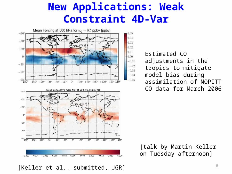
New Applications: Weak Constraint 4D-Var

Estimated CO adjustments in the tropics to mitigate model bias during assimilation of MOPITT CO data for March 2006

[Keller et al., submitted, JGR]

[talk by Martin Keller on Tuesday afternoon]

9

New Applications: 4D-Var Optimization of O3 Deposition

Mean a priori O3 bias (ppb)

Mean a posteriori O3 bias (ppb)

Ozone dry deposition velocity distribution

[Walker et al., submitted, JGR]

Inverse modeling of O3 deposition for August 2006 using AQS surface data

Background versus local anthropogenic contributions to Western US ozone pollution constrained by Aura TES and OMI observations

Investigation:Huang et al., JGR (in press) improved ozone source attribution by integrating Tropospheric Emission Spectrometer (TES) ozone and Ozone Monitoring Instrument (OMI) nitrogen dioxide into a state-of-the-art multi-scale assimilation system. Ozone attribution was estimated at surface monitoring sites when total ozone exceeded current and potential thresholds (Fig. c-d).

Key Findings:• Average background ozone was estimated at 48.3 ppbv or 76.7% of the total ozone in California-Nevada region in

summer 2008 (Fig. a-b) but was repartitioned between non-local pollution, which was enhanced by 3.3 ppbv from TES ozone assimilation, and local wildfires, which was reduced by 5.7 ppbv from OMI nitrogen dioxide assimilation.

• Background ozone varied spatially with higher values in many rural regions. Except Southern California, less than 10 ppbv of local anthropogenic ozone would be possible without violating a 60 ppbv threshold. Increases in non-local pollution and local wildfires will require additional reductions in local anthropogenic emissions to meet standards.

Science problem:Proposed reductions in EPA primary ozone standard increases the importance of accurate attribution of background (non-local and local natural) and local human ozone sources.

[Min Huang, JPL]

Comparison between 4D-Var and EnKF in CO2 flux estimation in TransCom regions with simulated GOSAT

Liu et al., 2015, in preparation

Black: truthBlue: prior fluxesRed: 4D-VarGreen: EnKF

EnKF

Monte Carlo method in 4D-Var

Monthly mean flux error reduction

Monthly mean flux error reduction

11 TransCom regions over land

• Comparable performance between EnKF and 4D-Var in CO2 flux estimation[Junjie Liu, JPL]

Now:• Current version matches one of

CT’s 16 flux scenario cases (MillerFossil,CASA-GFED2,TAKA-Interactive Atm fluxes)

Future work: • Residual modeling with EOFs

(MsTMIP uncertainty)• testing effect of filter window

length

Introducing GEOS-CarbonTracker (poster at GMAC 2015, Boulder)

[Andrew Schuh , CSU]

Based on EnKF approach

13

Developments Since IGC6

• Increase in the suite of observation operators for assimilation of satellite data• Nested full chemistry 4D-Var• Joint source/state optimization• Multispecies 4D-Var• Weak constraint 4D-Var• Monte Carlo and hybrid 4D-Var approach for Hessian calculation• GEOS-CarbonTracker

Future Challenges

• Data assimilation with the massively parallel GEOS-Chem• Enhancing availability of the EnKF capability to the GEOS-Chem community