d2.2.2 methodology and key performance indicators for...
TRANSCRIPT

SUNSEED, Grant agreement No. 619437 Page 1 of 66
D2.2.2 Methodology and key performance
indicators for resilient dense prosumer oriented DEG smart grid
energy and communications network

SUNSEED, Grant agreement No. 619437 Page 2 of 66
NOTICE The research leading to the results presented in the document has received funding from the European Community's 7th Framework Programme under the Grant Agreement number 619437. The content of this document reflects only the authors’ views. The European Commission is not liable for any use that may be made of the information contained herein. The contents of this document are the copyright of the SUNSEED consortium.

SUNSEED, Grant agreement No. 619437 Page 3 of 66
Document Information
1
PU Public
RP Restricted to other programme participants (including the Commission Services)
RE Restricted to a group specified by the consortium (including the Commission Services)
CO Confidential, only for members of the consortium (including the Commission Services)
Call identifier FP7-ICT-2013-11
Project acronym SUNSEED
Project full title Sustainable and robust networking for smart electricity distribution
Grant agreement number 619437
Deliverable number D2.2.2
WP / Task WP2 / T2.2
Type (distribution level)1 PU
Due date of deliverable 31.1.2016 (Month 24)
Date of delivery 30.1.2016 V1.0, updated 31.3.2016
Status, Version V2.0
Number of pages 66 pages
Responsible person, Affiliation Blaž Peternel, TS
Authors Blaž Peternel, Tomaž Lovrenčič, Niko Gamulin (TS), Jimmy Jessen Nielsen
(AAU), Ziming Zhu (TREL), Aleš Švigelj, Urban Kuhar, Kemal Alič (JSI) Pieter
H.A. Venemans (TNO), Jurij Jurše, (EP) , Bojan Miličič, (ES), Ljupco
Jorguseski, Casper van den Broek, (TNO), Saraansh Dave, Zhong Fan,
(TREL)
Reviewers Ljupco Jorguseski (TNO)

SUNSEED, Grant agreement No. 619437 Page 4 of 66
Revision history Version Date Author(s) Notes Status
0.1 30.10.2015 Tomaž Lovrenčič Initial data collection Pre-Draft
0.2 1.12.2015 Jimmy Jessen Nielsen Analysis of availability and latency KPIs of TS cellular networks
Pre-Draft
0.3 8.12.2015 Ziming Zhu Key performance metrics for converged network
Pre-Draft
0.4 5.1.20016 Ales Svigelj Data storage formats Draft
0.5 28.1.2016 Pieter H.A. Venemans Methods and tools Draft
0.5 28.1.2016 Ales Svigelj editing Draft
2.0 9.3.2016 Blaz Peternel Pre-final editing, TNO expertise on reliability added
Final Draft
2.0 15.3.2016 Herve Ganem Security KPI input Final Draft
2.0 16.3.2016 Blaž Peternel Final editing Final Draft for Review

SUNSEED, Grant agreement No. 619437 Page 5 of 66
Table of Contents Document Information ........................................................................................................................... 3
List of Figures ........................................................................................................................................... 7
List of Tables ............................................................................................................................................ 8
Abbreviations and acronyms ................................................................................................................... 9
SUNSEED project ................................................................................................................................... 11
1 Technical performance analysis and measures ............................................................................. 12
1.1 Power network key performance indicators ................................................................. 12
1.1.1 System indices ............................................................................................................... 12
1.1.2 KPI on SUNSEED use case Advanced distribution network management system platform 15
1.2 Communication network key performance indicators ................................................... 16
1.2.1 Physical network performance indices ......................................................................... 17
1.2.2 Logical network performance indices ........................................................................... 17
1.2.3 Techniques to achieve high reliability in communication networks ............................. 18
1.2.4 Analysis of Availability and Latency KPIs of TS cellular networks ................................. 19
1.3 Towards converged smart grid key performance indicators .......................................... 21
1.3.1 Reliability ....................................................................................................................... 21
1.3.2 Availability ..................................................................................................................... 23
1.3.3 User density ................................................................................................................... 24
1.3.4 Security .......................................................................................................................... 24
2 Economic performance analysis .................................................................................................... 25
2.1 Economic key performance indicators .......................................................................... 25
2.2 Business KPIs: Integration, installation, market considerations ..................................... 28
3 Methodology and evaluation of dense prosumer oriented DEG smart grid................................. 31
3.1 New methods and tools for assessing the reliability of smart grids ................................ 31
3.1.1 Introduction ................................................................................................................... 31
3.1.2 Performance indicators ................................................................................................. 31
3.1.3 Probability risk assessment ........................................................................................... 33
3.1.4 Basic principles of the proposed method ...................................................................... 33
3.1.5 Partial state space evaluation ....................................................................................... 35
3.1.6 Fault trees ...................................................................................................................... 35
3.1.7 Simulation and power flow analysis .............................................................................. 36
3.1.8 Architecture and design of a toolset ............................................................................. 37
3.1.9 Experiments with a trivial grid ....................................................................................... 43
3.1.10 Conclusions and plans for further work ........................................................................ 56
3.2 SG data collection ........................................................................................................ 58
3.2.1 Data storage/message format ....................................................................................... 58

SUNSEED, Grant agreement No. 619437 Page 6 of 66
4 References ..................................................................................................................................... 65

SUNSEED, Grant agreement No. 619437 Page 7 of 66
List of Figures
Figure 1: Possibility of KPI measurements in traditional power distribution network operation. ....... 15 Figure 2: KPI measurements in power distribution network operation on ADNMSP use case. ........... 16 Figure 3: Example cumulative distribution function (CDF) of latency and reliability. .......................... 18 Figure 4: Duration of outage events in cellular network per month. Horizontal dashed lines show the average mean time to repair (MTTR) over the whole year................................................................... 20 Figure 5: Round-trip time (RTT) statistics of cellular technologies. ...................................................... 20 Figure 6: Costs vs. volume curve. .......................................................................................................... 26 Figure 7: Costs of stand-alone and merged infrastructures. ................................................................. 27 Figure 8: Business case 1. ...................................................................................................................... 30 Figure 9: Set of Fault Trees (“Fault Forest”) .......................................................................................... 36 Figure 10: Architecture of the tool set .................................................................................................. 37 Figure 11: Optical path between nodes 14 and 5 ................................................................................. 39 Figure 12: Trivial network simulator ..................................................................................................... 42 Figure 13: Trivial test grid ...................................................................................................................... 43 Figure 14: Uncertainty as function of number of fault scenario's ........................................................ 53 Figure 15: Uncertainty as function of number of fault scenario's ........................................................ 53 Figure 16: Load692, phase B, passive mode ......................................................................................... 54 Figure 17: Load692, phase B, active mode ............................................................................................ 55 Figure 18: Load611, phase C, passive mode ......................................................................................... 55 Figure 19: Load611, phase C, active mode ............................................................................................ 56 Figure 20: Data structure. ..................................................................................................................... 59 Figure 21: An example of JSON structure for two nodes SPM data. ..................................................... 64

SUNSEED, Grant agreement No. 619437 Page 8 of 66
List of Tables
Table 1: Standard EN 50160 voltage characteristics with compliance limits – LV network [EN 2000]. 14 Table 2: Standard EN 50160 voltage characteristics with compliance limits – MV network [EN 2000]. ............................................................................................................................................................... 14 Table 3: Technology dependencies. ...................................................................................................... 19 Table 4: linear regression parameters of ping packet size to RTT mapping. ........................................ 21 Table 5: Business KPI stakeholders and key drivers. ............................................................................. 28 Table 6: Reliability values for selected countries .................................................................................. 32 Table 7: AMI measurement JSON structure. ......................................................................................... 60 Table 8: SPM measurement JSON structure. ......................................................................................... 61 Table 9: PMC measurement JSON structure. ......................................................................................... 62 Table 10: SE d JSON structure. ............................................................................................................... 62 Table 11: P/Q data JSON structure. ....................................................................................................... 63 Table 12: Short term load forecasting JSON structure. ......................................................................... 63

SUNSEED, Grant agreement No. 619437 Page 9 of 66
Abbreviations and acronyms
4G 4th generation mobile technology, LTE
2.5G 2.5th generation mobile technology, GPRS
ADSS All Dielectric Self Supporting combined optical and electrical cable
API Application Programming Interface
ARPU Average Revenue Per User
BSOTA Beyond State Of The Art
CBA Cost Benefit Analysis
CHP Combined Heat and Power
CIM Common Information Model
CPE Customer Premises’ Equipment, modem
CRAN Cloud Radio Access Network
CO2 Carbon Dioxide
DAP Data Aggregation Point
DEG Distributed Energy Generation
DEMS Distributed Energy Management System
DER Distributed Energy Resources
DG Distributed Generation
DMS Demand Management System
DR Demand Response
DSL Digital Subscriber Loop/Line
DSLAM Digital Subscriber Loop/Line Access Multiplexer
DSM Demand Side Management
DSO Distribution System Operator
DUT Device Under Test
DWDM Dense Wavelength Division Multiplexing
EMS Energy Management System
ENTSO-E The European Network of Transmission System Operators for Electricity
EV Electric Vehicle
FRR-A Frequency Restoration Reserve - Automatic
FRR-M Frequency Restoration Reserve - Manual
GPON Giga bit Passive Optical Network
GPRS General Packet Radio Service, 2.5G
GPS Global Positioning System
HV High Voltage, in power transmission lines, usually 110 kV or more
ICT IED (Intelligent Electronic Devices Information and Communication Technologies
IED Intelligent Electronic Devices
IPS Intrusion Prevention/Protection System
ISP Internet Service Provider
IT Information Technologies
KPI Key Performance Indicator
LAN Local Area Network
LAR Local Aggregation Router
LTE Long Term Evolution, 4G

SUNSEED, Grant agreement No. 619437 Page 10 of 66
LV Low Voltage, 240 V
Mb/s Mega bit per second, also abbreviated as Mbps
MIMO Multiple Input Multiple Output
MPLS Multi Protocol Label Switching
MSAN Multi Service Access Node
MV Medium Voltage, usually 10 kV or 20 kV
MVNO Mobile Virtual Network Operator
NIST National Institute of Standards and Technology
OFDM Orthogonal Frequency Division Multiplexing
OPCC Optical Phase Conductor combined optical and electrical cable
OPGW Optical Ground Wire combined optical and electrical cable
PGW Packet data Gateway in 4G
PLC Power Line Carrier or Communication
PV Photovoltaic
RAN Radio Access Network
RAR Remote Aggregation Router
RES Renewable Energy Sources
ROI Return On Investment
RTT Round Trip Time
SAIDI System Average Interruption Duration Index
SAIFI System Average Interruption Frequency Index
SCADA Supervisory Control and Data Acquisition
SDN Software Defined Network
SDP Service Delivery Point
SGW Signalling Gateway in 4G
SLA Service Level Agreement
SNR Signal to Noise Ratio
SOTA State Of The Art
TDM Time Division Multiplexing
TSO Transmission System Operator
Utility Distribution System Operator or energy retailer
V2G Vehicle to Grid
VPP Virtual Power Plant
VRF Virtual Routing and Forwarding
WAMS Wide Area Measurement System
WiFi Wireless Fidelity
WLAN Wireless LAN
xDSL X (= A – asymmetric, S – symmetric, V – very high bit rate) DSL
XML Extensible Markup Language

SUNSEED, Grant agreement No. 619437 Page 11 of 66
SUNSEED project
SUNSEED proposes an evolutionary approach to utilisation of already present communication networks from
both energy and telecom operators. These can be suitably connected to form a converged communication
infrastructure for future smart energy grids offering open services. Life cycle of such communication network
solutions consists of six steps: overlap, interconnect, interoperate, manage, plan and open. Joint
communication networking operations steps start with analysis of regional overlap of energy and
telecommunications operator infrastructures. Geographical overlap of energy and communications
infrastructures identifies vital DSO energy and support grid locations (e.g. distributed energy generators,
transformer substations, cabling, ducts) that are covered by both energy and telecom communication
networks. Coverage can be realised with known wireline (e.g. copper, fiber) or wireless and mobile (e.g. WiFi,
4G) technologies. Interconnection assures end-2-end secure communication on the physical layer between
energy and telecom, whereas interoperation provides network visibility and reach of smart grid nodes from
both operator (utility) sides. Monitoring, control and management gathers measurement data from wide area
of sensors and smart meters and assures stable distributed energy grid operation by using novel intelligent real
time analytical knowledge discovery methods. For full utilisation of future network planning, we will integrate
various public databases (e.g. municipality GIS, weather). Applications build on open standards (W3C) with
exposed application programming interfaces (API) to 3rd parties enable creation of new businesses related to
energy and communication sectors (e.g. virtual power plant operators, energy services providers for optimizing
home energy use) or enable public wireless access points (e.g. WiFi nodes at distributed energy generator
locations). SUNSEED life cycle steps promise much lower investments and total cost of ownership for future
smart energy grids with dense distributed energy generation and prosumer involvement.
Project Partners
1. TELEKOM SLOVENIJE D.D.; TS; Slovenia
2. AALBORG UNIVERSITET; AAU; Denmark
3. ELEKTRO PRIMORSKA, PODJETJE ZA DISTRIBUCIJO ELEKTRICNE ENERGIJE D.D.; EP; Slovenia
4. ELEKTROSERVISI, ENERGETIKA, MERILNI LABORATORIJ IN NEPREMICNINE D.D.; ES; Slovenia
5. INSTITUT JOZEF STEFAN; JSI; Slovenia
6. GEMALTO SA; GTOSA; France
7. GEMALTO M2M GMBH; GTOM2M; Germany
8. NEDERLANDSE ORGANISATIE VOOR TOEGEPAST NATUURWETENSCHAPPELIJK ONDERZOEK - TNO; TNO;
The Netherlands
9. TOSHIBA RESEARCH EUROPE LIMITED; TREL; United Kingdom
Project webpage
http://www.sunseed-fp7.eu/

SUNSEED, Grant agreement No. 619437 Page 12 of 66
1 Technical performance analysis and measures
1.1 Power network key performance indicators
DSO traditionally performs calculation on reliability and power quality KPI [PPA 2012], [WB 2009]. First one indicates the weakness of the network and stimulates DSO to build required reinforcements. Second, one analyses the voltage as a crucial electric parameter for power devices operation and also motivate DSO to implement network reinforcements and installation of proper compensation devices to keep voltage in prescribed limits. The further very important category is an operational KPI to directly determine the power system state parameters (e.g. voltage, current, power) which are then the basis for the calculation of some indirect KPI. Power loses are an example of this category. The total amount of them is closely linked with the cost for DSO. For that reason the DSO is highly stimulated to lower them with optimal comparison between network reinforcement on one side and energy price to power loses covering on the other [Galv 2011]. The data for reliability KPI calculation is at present only measured on the MV feeder level. This means that the number and the duration of outages in addition to total number of customers have to be identified on all MV feeders issuing from main supply substation. The power quality KPI is measuring, calculating and monitoring in main supply substations and switching stations which are included in SCADA system as remote terminal unit (RTU). For power quality KPI the special measurement analysing equipment is used. With SUNSEED concept realization the KPI will be determined even deeper alongside the MV feeder, e.g. on the MV/LV transformer station or its LV feeder level. With next generation smart grid distribution power network we see a transition when classical consumers and energy producers will start to act like prosumers. This means that they can influence on network operation with smart grid common elements like distributed generation, energy storage, microgrids, demand response capabilities. Power distribution network could operate with their support even some before highly important elements like main transformer or power lines dropped. This property of smart grid performance could also be measured by resiliency KPI which point to ability of network to operate in case of outages of supply transformers and main power lines.
1.1.1 System indices
1.1.1.1 KPI for Interruptions
The IEEE standard 1366 defines a number of system indices, i.e. KPI, for quantifying the availability of distribution grid [IEEE 2012]. In general interruption is defined as “the loss of service to one or more customers connected to the distribution portion of the system.”
1.1.1.1.1 KPI for standard interruptions
The following system KPIs are defined by the standard:
1. SAIFI - System Average Interruption Frequency Index. Defined as the ratio between the total number of customer interruptions and the total number of customers served from the system. The number of customer interruptions is defined as the sum, over all the interruptions during one year, of the number of customers affected by each interruption. (N interruptions during a year, with interruption i affecting Ci customers, Nc the total number of customers served). SAIFI measurement is mandatory.

SUNSEED, Grant agreement No. 619437 Page 13 of 66
𝑆𝐴𝐼𝐹𝐼 =𝑡𝑜𝑡𝑎𝑙 𝑛𝑢𝑚𝑏𝑒𝑟 𝑜𝑓 𝑐𝑢𝑠𝑡𝑜𝑚𝑒𝑟 𝑖𝑛𝑡𝑒𝑟𝑟𝑢𝑝𝑡𝑖𝑜𝑛𝑠
𝑡𝑜𝑡𝑎𝑙 𝑛𝑢𝑚𝑏𝑒𝑟 𝑜𝑓 𝑐𝑢𝑠𝑡𝑜𝑚𝑒𝑟𝑠 𝑠𝑒𝑟𝑣𝑒𝑑
2. SAIDI - System Average Interruption Duration Index. Defined as the ratio of the total interrupted customer minutes and the number of customers (Di the duration of interruption i). SAIDI measurement is mandatory.
𝑆𝐴𝐼𝐷𝐼 =𝑠𝑢𝑚 𝑜𝑓 𝑎𝑙𝑙 𝑐𝑢𝑠𝑡𝑜𝑚𝑒𝑟 𝑖𝑛𝑡𝑒𝑟𝑟𝑢𝑝𝑡𝑖𝑜𝑛 𝑑𝑢𝑟𝑎𝑡𝑖𝑜𝑛
𝑡𝑜𝑡𝑎𝑙 𝑛𝑢𝑚𝑏𝑒𝑟 𝑜𝑓 𝑐𝑢𝑠𝑡𝑜𝑚𝑒𝑟𝑠 𝑠𝑒𝑟𝑣𝑒𝑑
3. CAIDI - Customer Average Interruption Duration Index. Gives the average duration of an interruption as seen from a customer.
𝐶𝐴𝐼𝐷𝐼 =𝑠𝑢𝑚 𝑜𝑓 𝑎𝑙𝑙 𝑐𝑢𝑠𝑡𝑜𝑚𝑒𝑟 𝑖𝑛𝑡𝑒𝑟𝑟𝑢𝑝𝑡𝑖𝑜𝑛 𝑑𝑢𝑟𝑎𝑡𝑖𝑜𝑛
𝑡𝑜𝑡𝑎𝑙 𝑛𝑢𝑚𝑏𝑒𝑟 𝑜𝑓 𝑐𝑢𝑠𝑡𝑜𝑚𝑒𝑟 𝑖𝑛𝑡𝑒𝑟𝑟𝑢𝑝𝑡𝑖𝑜𝑛𝑠=
𝑆𝐴𝐼𝐷𝐼
𝑆𝐴𝐼𝐹𝐼
4. CTAIDI - Customer Total Average Interruption Duration Index. It only considers those customers that actually experienced an interruption during a certain year. It is defined as CAIDI, only with denominator is equal to the number of customers that experienced at least one interruption during a given year.
5. CAIFI - Customer Average Interruption Frequency Index. It quantifies the number of interruptions experienced by those customers that actually experienced interruptions. The value of the index indicates how much interruptions are experienced by a small group of customers.
𝐶𝐴𝐼𝐹𝐼 =𝑡𝑜𝑡𝑎𝑙 𝑛𝑢𝑚𝑏𝑒𝑟 𝑜𝑓 𝑐𝑢𝑠𝑡𝑜𝑚𝑒𝑟 𝑖𝑛𝑡𝑒𝑟𝑟𝑢𝑝𝑡𝑖𝑜𝑛𝑠
𝑡𝑜𝑡𝑎𝑙 𝑛𝑢𝑚𝑏𝑒𝑟 𝑜𝑓 𝑐𝑢𝑠𝑡𝑜𝑚𝑒𝑟 𝑤ℎ𝑜 ℎ𝑎𝑑 𝑎𝑡 𝑙𝑒𝑎𝑠𝑡 𝑜𝑛𝑒 𝑖𝑛𝑡𝑒𝑟𝑟𝑢𝑝𝑡𝑖𝑜𝑛
6. ASAI - Average Service Availability Index. It gives the average percentage of time during which a customer has electricity available.
7. ASIFI - Average System Interruption Frequency Index. Interruptions are weighted by the amount of load affected (Li be the load interrupted by interruption i and LT the total load supplied from the system).
8. ASIDI - Average System Interruption Duration Index. Interruptions are weighted by the amount of load affected.
9. CEMIn - Customers Experiencing Multiple Interruptions. It gives the fraction or percentage of customers that experience more than n interruptions.
10. ENS – Energy Not Supplied
1.1.1.1.2 KPI for short interruptions
KPI for short interruptions, i.e. momentary interruptions or a single opening/closing sequence of an interrupting device. The time between opening and closing should not exceed a maximum value, usually set at 5 min. Furthermore each momentary interruption event consists of one or more momentary interruptions. Duration-based classification is useful from customer point of view.
1. MAIFI - Momentary Average Interruption Frequency Index. It gives the count of momentary interruptions.
𝑀𝐴𝐼𝐹𝐼 =𝑡𝑜𝑡𝑎𝑙 𝑛𝑢𝑚𝑏𝑒𝑟 𝑜𝑓 𝑐𝑢𝑠𝑡𝑜𝑚𝑒𝑟 𝑖𝑛𝑡𝑒𝑟𝑟𝑢𝑝𝑡𝑖𝑜𝑛𝑠 𝑙𝑒𝑠𝑠 𝑡ℎ𝑎𝑛 𝑡ℎ𝑒 𝑑𝑒𝑓𝑖𝑛𝑒𝑑 𝑡𝑖𝑚𝑒
𝑡𝑜𝑡𝑎𝑙 𝑛𝑢𝑚𝑏𝑒𝑟 𝑜𝑓 𝑐𝑢𝑠𝑡𝑜𝑚𝑒𝑟𝑠 𝑠𝑒𝑟𝑣𝑒𝑑
2. MAIFIe - Momentary Average Interruption Event Frequency Index. It counts the number of momentary interruption events.
3. CEMSMIn - Customers Experiencing Multiple Sustained Interruptions and Momentary Interruption Events. It gives the fraction of customers that experience more than n sustained

SUNSEED, Grant agreement No. 619437 Page 14 of 66
interruptions and momentary interruption events. It takes into consideration both momentary and sustained interruptions.
1.1.1.2 Power quality indices
Power quality indices define voltage characteristics in distribution system and are based on standard EN 50160 [EN 2000]. Characteristics are summarised in Table 1.
Supply voltage characteristic Integral period
Measuring period
Statistical evaluation
Compliance limit
Supply voltage variations 10 min 1 week 95 % ± 10 %
10 min 1 week 100 % + 10 % / -15 %
Network frequency 10 s 1 week/year 95,5 % ± 1 %
10 s 1 week/year 100 % +4 % / -6 %
Flicker 2 h 1 week 95 % ≤ 1
Harmonics 10 min 1 week 95 % EN 50160
Voltage unbalance 10 min 1 week 95 % ≤ 2 %
Mains signalling voltage 3 s 1 day 99 % EN 50160
Table 1: Standard EN 50160 voltage characteristics with compliance limits – LV network [EN 2000].
Supply voltage characteristic Integral period
Measuring period
Statistical evaluation
Compliance limit
Supply voltage variations 10 min 1 week 99 % ± 10 %
10 min 1 week 100 % ± 15 %
Network frequency 10 s 1 week/year 95,5 % ± 1 %
10 s 1 week/year 100 % +4 % / -6 %
Flicker 2 h 1 week 95 % ≤ 1
Harmonics 10 min 1 week 95 % EN 50160
Voltage unbalance 10 min 1 week 95 % ≤ 2 %
Mains signalling voltage 3 s 1 day 99 % EN 50160
Table 2: Standard EN 50160 voltage characteristics with compliance limits – MV network [EN 2000].
1.1.1.3 Other meaningful KPI
The other KPI proposals also demonstrate novel approach in measuring efficiency of power distribution network. At this point they are only preliminary listed. They will be defined in detail in following phases of the project.
1. Operational KPI a. Power losses
2. Resiliency KPI. The idea of resiliency KPI is novel and it is beyond state of the art. The main conceptual difference in comparison with reliability KPI is that they are measured uptime instead of downtime. Network resiliency should become as important as network reliability and should be reflected in regulatory policies. The most difficult issue is not how to build the resiliency into the power supply but how to measure it.
3. Other: a. KPI for detection of voltage rise due to DER connection. b. Relation between total feed power amount from connected DER and consumer load
in the supply feeder.

SUNSEED, Grant agreement No. 619437 Page 15 of 66
1.1.2 KPI on SUNSEED use case Advanced distribution network management system
platform
With ADNMSP implementation the power distribution network becomes observable in all MV and LV electrical nodes and branches. In some characteristic locations the electrical parameters are measured with WAMS nodes and smart meters, on the others they are obtained with state estimations functionalities. This is undoubtedly new added value to make network operation more precisely and less risky to significant improve its efficiency. Prior to this, the electrical parameters were known only with SCADA measurements in the HV/MV main supply substation and MV switching station equipped with measuring and remote control equipment (Figure 1). For other network elements the parameter values had to be obtained only through separate the load flow analyses for some characteristic past or future network state.
0,4 kV
20 kV
20 kV
0,4 kV
0,4 kV
Feeder 20 kV SCADA
Transformer Station
20/0,4 kV
Transformer Station
20/0,4 kV
Transformer Station
20/0,4 kV
Main Supply Substation110/20 kV
Measurements (electric parameters, power quality, reliability) only on feeders issuing from HV/MV main supply substation (MDS) and MV switching station (SS) – RTU nodes
KPI determination only on the RTU nodes and MV feeder level
Measurements non presence alongside the MV and LV distribution network makes it impossible to DSO KPI determination
o Reliability KPIo Power quality KPIo Operational KPI
Figure 1: Possibility of KPI measurements in traditional power distribution network operation.
In fact, the greatly increased observability of the distribution networks enables the KPI detection in all MV and LV nodes and their connection branches (Figure 2).
It is reasonable to define the following KPI depending on the location in the power distribution network:
1) Busbars and feeders issuing from RTU substations (SCADA measurements)
a) Reliability KPI
b) Power Quality KPI
c) Operational KPI
2) Busbars and feeders issuing from transformer stations (WAMS node measurements)

SUNSEED, Grant agreement No. 619437 Page 16 of 66
a) Reliability KPI
b) Power Quality KPI
c) Operational KPI
3) Electrical nodes in MV and LV distribution network (WAMS node state estimation
measurements)
a) Operational KPI
4) Consumer, DER, EV charging station and prosumer nodes (WAMS node, smart meter
measurements)
a) Power Quality KPI
b) Operational KPI
Figure 2: KPI measurements in power distribution network operation on ADNMSP use case.
1.2 Communication network key performance indicators
Communication network performance monitoring is standard practice within telecom operator. Various network parameters are monitored in real time from communication equipment itself (e.g. via syslog or SNMP MIB) or is gathered via special monitoring nodes (Usually applied to end user QoS for IPTV and VoIP services.) [RFC3577], [RFC4150], [RFC4502], [RFC4711]. This is a well investigated topic, also for IPv6 networks [Bou 2004], [Cisc 2012], [Kuw 2013]. Below we present classical KPI that give information on the communication network quality on the physical layer.
0,4 kV
20 kV
0,4 kV
0,4 kV
Feeder 20 kV SCADA
Transformer Station
20/0,4 kV
Transformer Station
20/0,4 kV
Main Supply Substation110/20 kV
WAMS node instalation
Control box
Measured nodes
(WAMS, SCADA)
Measurements (electric parameters, power quality, reliability) on RTU, WAMS and smart meter nodes in power distribution network For other nodes alongside the MV and LV distribution network the measurements are made thruought state estimation.
Possibility of KPI determination on all MV and LV nodes and branches in power distribution network .
Estimated nodes (State Estimator)
o Reliability KPIo Power quality KPIo Operational KPI
o Reliability KPIo Power quality KPIo Operational KPI
o Reliability KPIo Power quality KPIo Operational KPI
o Power quality KPIo Operational KPI
o Power quality KPIo Operational KPI
o Operational KPI o Operational KPI
o Power quality KPIo Operational KPI

SUNSEED, Grant agreement No. 619437 Page 17 of 66
1.2.1 Physical network performance indices
Indices that describe performance on the physical communication layer are given below.
1. Latency or delay – The finite amount of time it takes a packet to reach the receiving endpoint after being transmitted from the sending endpoint. Telecom operators usually measure round trip time/delay (RTT), but certain services (e.g. WAMS, PMU) will require measurement of one-way delay, that necessitates time synchronization (e.g. NTPv4, GPS) between end points. To time synchronise measurements from WAMS nodes we implement time stamping of each measurement value. Time stamping must be centrally synchronised.
2. Jitter – The variation or the difference in the end-to-end delay between packets. Setting proper queue depth in upper layers of communication networks and minimizing number of communication nodes on end-2-end path minimizes jitter. WAMS nodes connected to mobile network will experience high jitter in communication path node – base station (e.g. > 20 ms in 4G).
3. Loss – A relative measure of the number of packets that were not received compared to the total number of packets transmitted. Loss is typically a function of availability. Most packet loss is usually experienced in access layer of communication network. Packet loss minimization is addressed by higher level protocols (e.g. TCP, message bus), but must be carefully applied since this increases jitter. To minimize loss, redundancy is employed, i.e. having two physical communication interfaces (e.g. fiber + 4G).
4. Availability – The fraction of time that network connectivity is available between an ingress point and a specified egress point, and defines network SLA. It directly influences service availability that defined as the fraction of time that service is available between a specified ingress point and a specified egress point within bounds of a defined SLA. One of the goals of DSO and telecom operator communication network convergence is to increase network availability.
5. Signal to Noise Ratio – It is the ratio between the maximum signal strength that a wireless connection can achieve and the noise present in the connection. Noise refers to the stray frequencies that interfere with the transmission of data in a wireless network. We will measure it at the cellular communication module.
1.2.2 Logical network performance indices
We are referring to IETF recommendations [RFC3577], [RFC4150], [RFC4502], [RFC4711]. These are implemented in relevant remote management systems (e.g. Nagios [Bar 2005]) and are implemented in a straightforward manner in existing communication network management centers. We have to assure that WAMS node is able to adhere to mentioned recommendations, i.e. from SNMP protocol to Syslog types of reporting, thus having enough processing and memory resources, as well as running operating system that implements such protocols by itself (e.g. Linux various distributions) [RFC5424], [RFC5674].
1.2.2.1 Reliability/availability of communication grid
Reliability/availability is typically referring to whether connectivity can be established or not. However, when considering a specific application with specific requirements, it makes more sense to define those KPIs as the ability of the end-to-end connection to fulfil the requirements posed by the application. However, as discussed in [Meti 2013], such a binary definition may not always be useful since in some cases an application may be able to work in a gracefully degraded mode, where it simply disables or postpones some advanced functionalities, but is able to continue operating the most crucial functionalities. In such cases it is much more useful to define a set of operational levels

SUNSEED, Grant agreement No. 619437 Page 18 of 66
for which the availability/reliability can be computed individually. A fictitious example of such can be seen in Figure 3, where the cumulative distribution of fictitious latency measurements is plotted (blue curve). Assume that two services are running, one requiring a maximum latency of 20 ms and the other with a less strict requirement of maximum 1 s of latency. The red dashed line indicates the strict requirement of 20 ms, and by reading of the corresponding level on the y axis, we can tell that the reliability of the strict service is approximately 82 %. For the other service whose maximum latency is 1 s, we can find that its reliability is 0.95, since this is where the blue curve becomes flat, and we know that in this example a packet loss of 5 % has been assumed.
Figure 3: Example cumulative distribution function (CDF) of latency and reliability.
1.2.2.2 User density
Another aspect that is not directly a measureable performance metric, but can have a big impact on the availability and reliability of a system is the supported number of users or density of users within a wireless coverage area. If for example a cellular network is able support all the required smart grid devices but it also has to serve regular users that may come/go and become active/inactive at random times, this varying load may cause that the strict requirements of the smart grid applications cannot be fully satisfied at all times. Therefore it makes sense to consider the degree of headroom in terms of number of active users and different types of load that the proposed smart grid communication system can support.
1.2.3 Techniques to achieve high reliability in communication networks
In traditional communication networks much functionality are built into the communication protocols at different layers in the protocol stack to ensure reliable communication. Some examples are: modulation scheme and bit-rate selection on physical layer, ARQ mechanisms on MAC and transport layers, QoS/ToS prioritization on the network layer and finally network coding on PHY/MAC or application layer. In addition to these techniques where the communication adapts to the conditions it is also important to ensure reliable conditions in the first place. The most straightforward way to increase reliability is to introduce redundancy in the least reliable components of a system. Concrete examples of redundancy would be a backup server that allows for server fail-over or additional physical cables or fibres that protects from single point of failure. A novel approach to ensuring highly reliable reporting from M2M devices is presented in [Corr 2014], where it is shown how LTE’s random access scheme can be reengineered to support periodic reporting and event based reporting with a guaranteed reliability level. For the SUNSEED project, a promising direction is to exploit that smart meters and WAMS nodes are expected to have multiple connectivity options such as PLC, xDSL, fiber, 2G, 3G, and 4G (LTE) and
0 5 10 15 20 25 30 35 400
0.1
0.2
0.3
0.4
0.5
0.6
0.7
0.8
0.9
1
latency −− x [ms]
F(x
)
Empirical CDF

SUNSEED, Grant agreement No. 619437 Page 19 of 66
possibly others, as mentioned above. A key property that can be exploited to increase reliability is to use redundant connectivity options that are as much as possible independent of each other, since this is a prerequisite for true redundancy. In Table 3 we list a number of possible resource failures (rows) and some different connectivity options (columns). In the table we show to which extend the different connectivity options are affected by the failures and to which extend they will fail simultaneously or independently.
Resource \ technology PLC Cable xDSL FTTH 2G 3G 4G Wi-Fi mesh
House power X limited, device could use battery
BS - power outage
X
BS - specific modem down
X X X
Cables in road/sidewalk break potentially in same duct
Telecom DHCP, DNS down
potentially shared
Telecom core down
Probably shared if same telecom
Neighbourhood blackout X
limited, could use battery
Table 3: Technology dependencies.
1.2.4 Analysis of Availability and Latency KPIs of TS cellular networks
In this section a preliminary study of availability and latency performance of TS’ cellular networks is presented. The study is based on measurements taken between June 2014 and May 2015.
1.2.4.1 Availability and failure event duration
Initially we present the observed average availability of different types of network elements. For example, in week 5 of 2015 these numbers looked as follows [%]:
HLR MSCS MGW SGSN GGSN BSC RNC TSCS GSM BST UMTS BST LTE BST
100 100 100 100 100 99,995 100 100 99,5634 99,5102 99,8692
While the numbers are quite similar for GSM and UMTS and to some extent LTE, the three technologies may in some cases have failed independently of each other, while in other cases the failures are completely correlated. Correlated/simultaneous failures can happen when a tower hosting multiple technologies collapses, if it is covered in ice due to sleet, or it loses power and backup power. In order to understand the outage event measurements, we have used information about 1) the average duration (per month) of outage events, and 2) the number of events per month, to find the average duration of failure events. This has been calculated for each of the considered cellular technologies and is presented in Figure 4. The average event duration is calculated as the total outage time per month divided by the number of events per month. Additionally we show the average mean time to repair (MTTR), which is calculated as the mean of each of the 3 plots. From the figure it is clear that the three technologies have similar average values of MTTR of approximately 200 min/event.

SUNSEED, Grant agreement No. 619437 Page 20 of 66
Figure 4: Duration of outage events in cellular network per month. Horizontal dashed lines show the average mean time to repair (MTTR) over the whole year.
1.2.4.2 Latency of cellular technologies
For the different available cellular technologies, ping measurements from the field of varying packet sizes have been conducted regularly on a daily basis. Based on such measurements from Jun-14 to May-15 (except LTE where measurements were not available until Feb-15), we have calculated the average round-trip time for each cellular technology and for the different packet sizes. These calculated numbers are shown in Figure 5, where a clear linear relationship is visible.
Figure 5: Round-trip time (RTT) statistics of cellular technologies.
Jun-14 Jul-14 Aug-14 Sep-14 Oct-14 Nov-14 Dec-14 Jan-15 Feb-15 Mar-15 Apr-15 May-150
50
100
150
200
250
300
350
400
450
500
Eve
nt
du
ratio
n [m
in]
GSMGSM MTTRUMTSUMTS MTTRLTELTE MTTR
32 200 800 1500
Packet size [Bytes]
0
200
400
600
800
1000
1200
1400
RT
T [
ms]
GPRSEDGEUMTSHSDPALTE

SUNSEED, Grant agreement No. 619437 Page 21 of 66
Based on the derived ping statistics in Figure 5 we have approximated linear regressions of the relationship between packet size and RTT for the five technologies. That is, the mean RTT is given as [ms]:
𝑅𝑇𝑇 = 𝛼 ∙ 𝐵 + 𝛽 where B is the ping packet size in bytes, and further 𝛼 and 𝛽 are the technology-specific parameters of the linear regression, given in Table 4.
Table 4: linear regression parameters of ping packet size to RTT mapping.
The plot shows clearly the evolution in cellular technologies, where the oldest 2G technology GPRS is significantly slower than the 2.5G – 3G – 3.5G technologies EDGE, UMTS and HSDPA, and the newest 4G technology LTE is superior to the rest with a very low and almost packet size independent transmission delay.
1.3 Towards converged smart grid key performance indicators
1.3.1 Reliability
1.3.1.1 Packet loss
A typical parameter used in communication networks to quantify the communication link reliability is the packet loss ratio (PLR) measured on a particular protocol layer between the communication source and destination. The PLR is defined as follows: PLR = (nr_packets_sent – nr_packets_suc_received)/nr_packets_sent where nr_packets_sent : the number of packets sent by the communication source nr_packets_suc_received : the number of packets successfully received at the communication destination However, this PLR definition cannot be simply re-used from smart grid’s perspective, as it does not relate to the transmitted message type and its corresponding latency requirement as defined in D3.1. Additionally, the payload of the transmitted message between the two nodes (and their respective smart grid functions) might be segmented over a several packets at a particular protocol layer. This segmentation should be also considered in the communication link reliability requirements definition for SUNSEED. Therefore, the communication link reliability requirement CLRmessage in SUNSEED is defined based on the transmitted message type at the smart grid (management) application layer and the corresponding message latency requirement Dth,message for proper functioning of the particular application (or function), as follows:

SUNSEED, Grant agreement No. 619437 Page 22 of 66
CLRmessage = nr_messages_received (T < Dth,message) / nr_message_sent > CLRth,message
Note here that nr_messages_received (T < Dth,message) is the number of messages arriving at the communication destination within the latency requirement while nr_messages_sent is the total number of messages sent by the communication source. This definition is from the end-to-end communication perspective and therefore intermediate packet segmentations, losses and retransmissions (if applicable) on a particular communication link’s segment and protocol layer will affect the total message delay. The CLRmessage requirements vary with the nodes type and the function (or application) running on these nodes. For example, end nodes like PMU, SM, and WAMS running non-critical smart grid applications are typically having lower CLRmessage requirements (e.g. down to 1% or 0.1%). Other control nodes such as voltage regulators, circuit breakers, switches, etc. have higher CLR requirements (e.g. four-to-five nines).
1.3.1.2 Latency
The finite amount of time it takes a packet to reach the receiving endpoint after being transmitted from the sending endpoint. Telecom operators usually measure round trip time/delay (RTT), but certain services (e.g. WAMS, PMU) will require measurement of one-way delay, that necessitates time synchronization (e.g. NTPv4, GPS) between end points. To time synchronise measurements from WAMS nodes we implement time stamping of each measurement value. Time stamping is centrally synchronised. The SUNSEED’s formal definition of the communication latency requirement follows the definition in [IEC61850]. Note that the latency requirement is defined between two physical nodes running a particular smart-grid management function or application. For example, a SM or WAMS node (as a source) running a measurement functionality sending measurement reports to the smart-grid management node (as a destination) running a grid state estimation function. The latency requirement is then defined as: T = ta + tb + tc < DTh,message , where ta and tc are the delays for processing the message at the source and destination, respectively; tb is the communication link delay between the source and destination Dth,message is the required message delay that depends on the detailed metering and WAMS applications, for example: 1) PMU related latency requirements: 8 - 100 ms (depend on individual message types)
2) SM related latency requirements (AMI) : 1 s
3) WAMS related latency requirements: 100 - 200 ms
1.3.1.3 Jitter
The variation or the difference in the end-to-end delay between packets. Setting proper queue depth in upper layers of communication networks and minimizing number of communication nodes on end-2-end path minimizes jitter. In SUNSEED, we plan to connect the WAMS directly to access and/or aggregation layer of communication network without intermediate multiplexers (as in PLC) to minimize jitter. Mobile networks experience high jitter in communication path node – base station (e.g. > 20 ms in 4G) and may not be suitable for conveying information for most demanding low latency tasks.
1.3.1.4 Signal to Noise Ratio

SUNSEED, Grant agreement No. 619437 Page 23 of 66
It is the ratio between the maximum signal strength that a wireless connection can achieve and the noise present in the connection. Noise refers to the stray frequencies that interfere with the transmission of data in a wireless network. In the field trial, we measure the signal to noise ratio at the location of every cellular communication module to ensure that the ratio falls in an acceptable level.
1.3.2 Availability
The fraction of time that network connectivity is available between an ingress point and a specified egress point, and defines network availability. It directly influences service availability that defined as the fraction of time that service is available between a specified ingress point and a specified egress point within bounds of a defined network availability. One of the goals of DSO and telecom operator communication network convergence is to increase network availability.
For the overall smart grid communications system reliability analysis there is a need of node reliability and availability definitions in the time and spatial domain. Note that the node reliability definition is typically based on two important metrics, namely Mean Time Between Failure (MTBF) as the average time between node failures, and Mean Time To Repair (MTTR) as the average time needed for the node in outage to be repaired and become operational. These MTBF and MTTR node reliability metrics are needed for the two coupled systems: a) The nodes in the electricity distribution system: SM nodes, WAMS nodes, grid control station/server nodes, etc.
b) The nodes in the overlapped communication system: communication modems in SM and WAMS, base stations, PLC concentrators and relays, core network nodes in cellular networks (e.g. BSCs/RNCs, P- or S-GW, SGSN/GGSN, HLR), routers/switches fixed networks, etc. Next to the MTBF and MTTR input for the node reliability, it is important to know from overall smart grid system reliability about the spatial domain impact if outage occurs at particular node. For example, consider the possible outage of the PLC concentrator node or a base station, which both have a MTTR of about e.g. few hours. An outage of the PLC concentrator will cause that all nodes connected to it e.g. on a street level are unavailable for communication (e.g. effectively in outage) while if a base station outage occurs then all nodes connected to it on a neighbourhood level are unavailable for communication (e.g. effectively in outage). On a more global scale, assume that some of the core nodes (e.g. BSC/RNC, gateways, switches, routers, etc.) are having an outage, which e.g. is once per few years and their repair is typically within few hours. These core nodes are supporting many end-nodes and therefore have a larger spatial impact on the communication unavailability (or outage) for example on the city, district/province or even country level. Another extreme are very short outages on a scale of several milliseconds or seconds of a single node (e.g. SM, WAMS, etc.) for example due to unexpected interference, software updates/reboot, etc. In electricity distribution systems typical availability performance metrics are the System Average Interruption Frequency Index (SAIFI) and System Average Interruption Duration Index (SAIDI). SAIFI is the average total number of interruptions that a customer would experience in a period of one year. SAIDI is the average outage duration for each customer served. In the SUNSEED system reliability analysis the MTBF and MTTR reliability metrics (as these are specific per particular node) will be calculated from these tables and complemented with results found in the literature.

SUNSEED, Grant agreement No. 619437 Page 24 of 66
In future smart grid environments the availability of the supporting communication network is crucial, as there will be a high proportion of population integrated in the smart grid as electricity prosumers. The availability is a degree to which the system, element or component is operational and accessible when required to be used and is defined as: Availability [%] = MTBF / (MTBF + MTTR) For the purposes of communication networks, availability can also be expressed as hours per year of downtime. MTBF is statistically established metric, on the field with large population of elements over a longer period. MTTR is statistically measured metric on the field and it is the repair time until the reestablishment of the normal operation of particular node/element. All times is sum of unplanned downtimes and scheduled maintenance times. Packets loss is also a function of availability. Most packet loss is usually experienced in access layer of communication network. Packet loss minimization is addressed by higher level protocols (e.g. TCP, message bus), but must be carefully applied since this increases jitter. In SUNSEED, taking the advantage of heterogeneous networks provided by the telecom, we consider having two physical communication interfaces (e.g. fiber + 4G) in order to enable maximal availability.
1.3.3 User density
Another aspect that is not directly a measureable performance metric, but can have a big impact on the availability and reliability of a system is the supported number of users or density of users within a wireless coverage area. If for example a cellular network is able support all the required smart grid devices but it also has to serve regular users that may come/go and become active/inactive at random times, this varying load may cause that the strict requirements of the smart grid applications cannot be fully satisfied at all times. Therefore it makes sense to consider the degree of headroom in terms of number of active users and different types of load that the proposed smart grid communication system can support. Discussions on the relation between the performance of the cellular network and the number of users are seen in D3.1 and D3.2.1.
1.3.4 Security
The security requirements was identified in D2.1.1, according to the security and privacy group of the Smart Energy Collective [2], NIST [Nist10] and the analysis of the SUNSEED use cases. In particular for SUNSEED. The criteria used to evaluate the security solutions will be as follows; End to end security: SunSeed involves multiple use case scenarios corresponding to a number of communication schemes, involving single or multihop communications. We want to achieve end to end security at least in the sense that every hop in SUNSED communication schemes should be protected by the use of credentials. . The data protection involves authenticated and authorized data access insuring data integrity and data confidentiality and should be compatible with security standards defined in IEC 62351 Furthermore, the security solution selected should enable , when required to implement end to end data protection at the applicative level from source to destination with a single set of credentials, opening the possibility for transmitted data to transit via platforms not necessarily trusted Another aspect of the security evaluation is related to the ability to grant/revoke dynamically access rights to access controlled resources.

SUNSEED, Grant agreement No. 619437 Page 25 of 66
2 Economic performance analysis
Telecommunications encompasses several ICT domains, each with its own set of infrastructure types, for example: communication networks, servers, storage, and software for data analysis. Telecommunications also need standards and protocols. But these facts are more or less independently of the several different market. This assumption is very important when we what put telecommunication services in that markets. Logical conclusions are that we can construct different telecommunication structures for demand of each of those markets with more or less the same or very similar assets. Can we merge two different demands for telecommunication services of two different markets? That is, can we merge demands from energy distribution utility market and telecommunication market? If the answer is yes, under certain assumptions, then we can construct converged communication infrastructure that can suit both markets and stakeholders well. On one side we gain larger volumes, due to merged markets (electricity distribution, telecommunication services) and lower costs, due to these larger volumes, but at the same time achieve also lower operational costs due to merged infrastructures, i.e. communication networks with all support infrastructures, too (e.g. procurement of equipment, data center, billing chain, call center, software licenses).
2.1 Economic key performance indicators
We introduce some classical microeconomics and cost theory and refer to other sources for deeper coverage of pricing of telecommunication networks [Cour 2003], [Keen 2010], [Small 2014], [Vandi 2014]. Let us start with basic, but very important facts. The first is definition of total costs.
𝑇𝑜𝑡𝑎𝑙 𝑐𝑜𝑠𝑡𝑠 = 𝑓𝑖𝑥𝑒𝑑 𝑐𝑜𝑠𝑡𝑠 + 𝑣𝑎𝑟𝑖𝑎𝑏𝑙𝑒 𝑐𝑜𝑠𝑡𝑠
The second is that costs are a function of economics of scale (Figure 2). This means that every additional unit allocate less costs then previous one. Unit in that case has universal meaning (e.g. bit, bit/s, MByte, Mbit/s, TByte, Gbit/s).

SUNSEED, Grant agreement No. 619437 Page 26 of 66
Costs
Volume
Incremental costs for aditional
unit
Costs of previous unit
Aditional
unit
Previous
unit
Figure 6: Costs vs. volume curve.
The third is that costs are sum of depreciation, costs of capital and operational expenditure.
𝐶𝑜𝑠𝑡𝑠 = 𝐷𝑒𝑝𝑟𝑒𝑐𝑖𝑎𝑡𝑖𝑜𝑛 + 𝐶𝑜𝑠𝑡𝑠 𝑜𝑓 𝑐𝑎𝑝𝑖𝑡𝑎𝑙 + 𝑂𝑝𝑒𝑟𝑎𝑡𝑖𝑜𝑛𝑎𝑙 𝑒𝑥𝑝𝑒𝑛𝑑𝑖𝑡𝑢𝑟𝑒
Costs mentioned in equation above can have fixed or variable nature of cost in observed time. So, we can construct function of costs depending on volumes (Figure 7). The fourth is that costs are function assets and not function of ownership of assets. For example, Operational expenditures for maintenance of optical fibres are just function of:
1. Quality of materials. 2. Construction.
If we consider all facts mentioned above we get conclusion that merged telecommunication infrastructure for more than one market required less costs per unit compared with stand-alone situation. In Figure 7 A case presents merged situation and B case stand-alone situation.

SUNSEED, Grant agreement No. 619437 Page 27 of 66
Costs
Volume
Incremental costs of
Telco's infrastructure on
Electric market
Stand-alone costs of Telco's
infrastructure on only
telecomunication market
Volume of
telecomunication
services on electric
market
Volume of
telecomunication
services on
telecomunication
market
Figure A
Costs
Volume
Stand-alone costs of DSO-
TSO's telecomunication
infrastructure on electric
market
Volume of
telecomunication
services on electric
market
Figure B
Figure 7: Costs of stand-alone and merged infrastructures.
Suitable KPI can be incremental vs. standalone costs for telecommunication demand on electric market on different level, region or business function demands [Alle 2002]. We can measure KPI in the way that observe how many money we spent for construction the telecommunication infrastructure (investment amount, depreciation and cost of capital) and how many money yearly we spent for operation (operational expenditure). The communication network means investment into cable and mobile infrastructure. Investment into cable infrastructure means construct the cable networks and connect this with telecommunication equipment together on one side. On the other side we need to construct access network for purpose of connect users to telecommunication network. Investment into mobile infrastructure means construct mobile network with many base stations to cover region with radio signals. When we connect mobile communication equipment together we get mobile infrastructure. We construct base station access network for purpose of access users to mobile telecommunication network.

SUNSEED, Grant agreement No. 619437 Page 28 of 66
Degree of the development of fixed or mobile network means how much the access network is wide spread over the region or state. The main questions into costs of telecommunication activity are:
a) Costs of access to telecommunication services from user geographically coordinate to the closer connection point on the telecommunication side.
b) Costs of operations for different services.
Above was mentioned that economic increment means additional cost for additional service. In the project we can measure:
a) Additional costs for access to telecommunication network compared two situations (Figure 3 A and B).
b) Costs of operations for services in both situations (Figure 3 A and B).
When in our modelling approach we include time, we get long run incremental cost model (LRIC). We can construct model for A and B situation.
2.2 Business KPIs: Integration, installation, market considerations
Smart grid initiatives aim to leverage communication capability coupled with sensor networks to achieve multiple goals, such as, improving efficiency and utilisation of assets and creating a dynamic load base [IEEESG 2013]. In the scenario where communication networks are integrated with a distribution network operator, the additional real-time information enables the DSO (or DNO) to reduce asset expenditure and provide new services (e.g. demand side management). The SUNSEED project aims to investigate and trial a number of these use cases in order to understand the costs and benefits (both technical and economic) of leveraging existing telecommunication networks to achieve better efficiency and utilisation of assets. Bringing these traditionally separate industries together under the smart grid name increases the number of stakeholders that need to be satisfied. The table below outlines the key stakeholders from the SUNSEED use cases, as well as an outline into their key drivers.
Stakeholders Key drivers
Distribution Service Operator Efficient use of resources and avoid capital cost. Demand side management measures to aid in managing the network. Meeting regulatory requirements and obligations in terms of network downtime, security, and reliability.
Telecommunications Service Operator
Leveraging networks for smart grid applications. Meeting regulatory obligations.
Consumer Maintaining a certain level of comfort. Low cost for electricity. Security of supply. Ability to produce and consume electricity.
Regulator Maintaining an acceptable quality of service. Short and long term security of supply. Driving change through policy/regulatory methods.
Technology providers Developing scalable solutions for smart grid applications. Demonstrating benefits of sensor information to manage infrastructure/networks. Tackling real-world issues such as security for critical infrastructure applications.
Table 5: Business KPI stakeholders and key drivers.

SUNSEED, Grant agreement No. 619437 Page 29 of 66
Having discussed the key stakeholders and presented a brief outline into their main drivers, some performance indicators can be developed to quantify the impact on the key drivers of adopting smart grid solutions. Using communication technology to improve asset utilisation can be measured by:
Communications cost (Ccomm) – the total cost of deploying/reengineering a communication network for a given application.
Business as usual cost (Cbau) - the traditional cost of implementing this solution.
Capacity released by installing communications (Pcomm) – the extra capacity that is gained by installing communications systems.
Capacity released by using traditional solutions (Pbau) - the extra capacity that is gained by business as usual solutions.
This will then allow for an estimate of EUR per MW for each method; business as usual or smart grid approach (Cother is the other, non-communications related, costs associated with the smart grid approach).
𝛼 =(𝐶𝑐𝑜𝑚𝑚 + 𝐶𝑜𝑡ℎ𝑒𝑟)
𝑃𝑐𝑜𝑚𝑚
𝛼′ =(𝐶𝑏𝑎𝑢)
𝑃𝑏𝑎𝑢
This provides comparable ratios for the proposed method (i.e. leveraging communications networks) against the traditional approach which may include network reinforcement. This helps address the business metrics for both the DSO and TSO when looking at system level solutions. To complement these estimates, other figures will also be required for the proposed solution; network downtime and customer hours lost such that the reliability of the proposed approach is validated. To address consumer drivers of reliable supply and cost implications, the following measures may be appropriate:
Customer hours lost
Cost implications for consumers of the proposed method versus business as usual
Sensor networks also allow for greater predictability of network behaviour, however it is not decided what level of sensor coverage (e.g. 10 % or 90 %) is required to improve predictability significantly. Again, another measure is proposed where we calculate:
The marginal effect of adding an extra sensor in terms of improvement on predictability. The cost implication is both in the deployment of sensors as well as the cost in transporting, storing, and processing the data.
The above mentioned concepts and measures can be applied for each use case individually to ascertain which solutions have the greatest impact and how they compare to traditional methods of system operation. Include business case where many prosumers are activated

SUNSEED, Grant agreement No. 619437 Page 30 of 66
Figure 8: Business case 1.

SUNSEED, Grant agreement No. 619437 Page 31 of 66
3 Methodology and evaluation of dense prosumer oriented DEG
smart grid
3.1 New methods and tools for assessing the reliability of smart
grids
3.1.1 Introduction
The SunSeed project is a collaborative initiative to develop the technology and gain experience by upgrading an existing power distribution grid into a “smart grid” that includes distributed generation, extensive monitoring facilities and real-time control. The required datacommunication services are, as far as possible, implemented using the existing telecommunications infrastructure. One of the central research questions of this project is whether the converged infrastructures of DSO and telecom operator can result in a power distribution system that meets all performance requirements (availability, robustness etc) for such systems. This is non-trivial, especially since an (existing) public telecom infrastructure is typically not designed with the requirements of a power distribution network in mind. In addition, the reliability of many IT components (servers, data bases etc) may not be comparable to the high reliability of power components. Hence, robustness and fault-tolerance are important aspects that have to be taken into account during the design phase of the smart grid. High robustness can be realised by using high-reliability components, employing sufficient redundancy and/or by limiting the impact of failures in other ways. A good methodology and a set of supporting tools to assess the consequences of design decisions on the expected reliability and performance is therefore very important. Typical control schemes in Smart Grids include feedback control (for instance to switch off the charging of electric vehicles when voltage drops) and this makes it non-trivial to assess the impact of failures on the stability and hence the reliability of the complete system. This feedback nature prevents us from calculating the reliability of the energy grid and the ICT layers separately and combine the values in some way or another. This chapter described a method that treats the Smart Grid as a whole, not as the sum of its parts. Some general aspects of combining power and communication network simulations and an overview of some existing tools can be found in [Met14] First, we will describe the theory behind the proposed method. This is, in part, based on [Ven12]. Then we will describe the architecture and design of a set of tools that implement the proposed method. This tool set is currently in the process of being implemented, so experimental results will only be available in a later stage. However, we will describe a very simple and trivial test scenario. The only purpose of this scenario is for testing the tool set and for performing some experiments. In a later stage, more test scenarios will be created, possibly focussed on the SunSeed field test.
3.1.2 Performance indicators
“Availability” or “Security of supply” is an important key performance indicator (KPI) of Smart Grids. It is a measure for the ability of the system to transport energy to its customers without interruptions and is usually defined as a time fraction (such as 99.999%). Other related performance indicators are the number of outages per time unit (i.e. year) and the (average) duration of outages. Combined with

SUNSEED, Grant agreement No. 619437 Page 32 of 66
data regarding numbers of customers we can calculate various KPI’s, such as defined by EN-50160 [Cen94] and IEEE-1366 [IEEE11] The main reliability KPI’s are:
SAIFI – System Average Interruption Frequency Index
CAIDI – Customer Average Interruption Duration Index
SAIDI – System Average Interruption Duration Index They are defined as follows: SAIFI = (Total number of customer interruptions) / (Total number of customers served) CAIDI = (Sum of customer interruption durations) / (Total number of customer interruptions) SAIDI = (Sum of customer interruption durations ) / (Total number of customers served)
Obviously, SAIDI = SAIFI × CAIDI and is often expressed as a percentage. For example, an average interuption duration of 1 hour per year implies an availability of 99.988% Typical SAIDI and SAIFI values as they are realized over the world can be found in the following table
[Nel11]
Table 6: Reliability values for selected countries
Apart from the EN-50160 parameters. there are other performance indicators that may be considered important [Dup10]:
Demand and Supply balancing: the percentage of time that the demand and supply deviate from each other.
Avoidance of peaks as a measure of the effectiveness of demand management.
Efficiency of delivery, being the ratio of the consumption of locally generated energy and the total consumption of energy.
Environmental impact, being an indicator to what level “green” energy sources are used.

SUNSEED, Grant agreement No. 619437 Page 33 of 66
Service offering, for example the probability that an electric vehicle is charged in time.
Service fairness: an indicator to which extend all distributed energy generators have been granted the right to deliver power to the grid.
In this chapter, we will concentrate on ’availability’ (SAIFI × CAIDI), but the same methodology can also be used to quantify other performance indicators. For example, a similar method that was used to evaluate designs for telecommunication backbone infrastructure were able to provide values for quantities comparable to SAIFI and CAIDI individually (not only their product).
3.1.3 Probability risk assessment
“Probability Risk Assessment” is the common name for the evaluation of risks associated with a complex engineered technological entity in a systematic and comprehensive way [Cia10], [Cia09]. Calculation of the expected availability of a system can be performed in different ways:
Analytically. When failure causes are statistically independent and the system is relatively simple, logical operators can be used to combine failures of individual systems, elements, and components into the failure of a service and calculate the probabilities.
By simulation. When failure causes are not statistically independent or failures have non-trivial and interdependent causes, then analytical methods may not be possible and simulation may prove an alternative. Simulation is often costly in terms of time, computational and software resources.
One common method for simulating a system that includes stochastic variables is the Monte Carlo method. With this method, random inputs are drawn from the probability distributions of the stochastic variables and the outcome of the system is calculated for these inputs. This is repeated many times and in the end, all results are aggregated. A fundamental problem with Monte Carlo is that a very large number of random draws may be required before the effects of certain rare events become visible (such as the failure of a very reliable component). Rare Event Simulations involves estimating probabilities of events that occur very infrequently but have consequences that are significant enough to justify their study. The method proposed here combines these principles and uses:
(1) Analytical calculations by means of Fault Tree Analysis, (2) Partial State Space evaluation and (3) Simulation of semi-stationary fault scenarios.
3.1.4 Basic principles of the proposed method
The fundamental assumption underlying the proposed method is that the operating state of a Smart Grid is determined by a finite number of external factors such as spontaneous hardware failures, damaged cables, flooding etc. Those are the “root causes” that may cause one or more elements of the system to malfunction. The system can then be seen as always operating in one of a discrete number of failure states, each state being a certain combination of root causes. A large class of external influences are formed by the spontaneous failures of individual elements, like switches, transformers, cables, routers etc., but there may be others that have impact on groups of elements, like fire in a power distribution station or the failure of a GSM transmission tower. Note that failures of elements due to overload are not considered as “root causes”: their failure is probably the results of a chain of events that have a different root cause.

SUNSEED, Grant agreement No. 619437 Page 34 of 66
For the sake of simplicity, we will assume here that all external influences are bi-modal: true or false. Later this assumption can be broadened to allow multi-model effects, such as the outside temperature or the amount of wind and sunlight (continuous quantities, like temperature, can be discretized). Assume there are N external root causes. Particular state j of the system will be written here as vector:
),...,,( ,,2,1 jNjjj sssS
with jis , representing the state of root cause i in system state j.
The total state space is the (finite) set of all possible states and will be written as S. The number of elements in the set can become very large: with N bi-modal root causes, the number of states is equal to 2N. We will also assume that is possible to calculate (or at least estimate) probability Pj of state j. When the elements si are all statistically independent, we can calculate Pj from the probabilities of the element states si:
N
i
jiij ssPP1
, )(
Next we have to define quantity G that we want to use to evaluate the performance of the system, for instance the fraction of the time (or probability) that the energy demand of a given customer can be fulfilled. We assume that we can define a function g(S) that maps every state S to a certain (binary) outcome, i.e. whether the customer demand can be fulfilled or not. A further assumption is that the outcome g in a certain state only depends on the state vector S and not on the previous state(s). In other words, the system states are supposed to be memoryless. In order to fulfil this assumption, it may be necessary to model any “memory” effects as external influences (and include them in state vector S). Determining the value of g(S) may not be trivial as it may involve evaluating the effects of failure chains, protection mechanisms and corrective actions by control units. For instance, a single damaged cable may cause other elements to be overloaded or switched off by protection mechanisms etc. We will assume here that such a chain of events will always lead to a stationary situation for which the value of g(S) can be determined. With this function g, it is now possible to calculate the expected value of the desired quantity G as a weighted sum:
N
j
jj SgPGE2
1
)()(
Calculating this weighted sum may be problematic in practice as the size of set S may be very large and calculating g(Sj) for each state Sj can be time consuming.

SUNSEED, Grant agreement No. 619437 Page 35 of 66
3.1.5 Partial state space evaluation
The computational complexity of calculating the weighted sum G can be reduced by only evaluating a subset S’ of S. Assume W to be the set of all possible values of j (1...2N). Then let V be the subset of all
indices of the states in S’: S’ = { Sj } for all jV. Then G can be calculated as follows:
Vj
jj SgPGE )()(
with ε indicating the approximation error. The maximum error that is made can be calculated by a worst/best case analysis: in the best case, g evaluates to true (or 1) for all states in S-S’, in the worst case it evaluates to false (or 0) for those states. Hence:
VWj
jP\
0
The subset S’ should be chosen wisely: in order to minimize the error, the sum of the probabilities of the excluded states should be smaller than the allowed inaccuracy of the results. At the same time, we want to minimize the number of states in S’ in order to keep the computation time limited. The optimal solution is to sort all elements of S according to their probability and choose subset S’ from the states with the highest probability, up till the desired accuracy is reached. However, this can be impractical since the number of states in S can be too large to sort. Therefore, we apply some heuristic methods to select the states for S’ by enumerating them in a roughly-sorted order. First step is to select states with an increasing number of failures. The first state is the failure-free state, then all states with exactly one failure, then all states with exactly two failures etc. Since failure probabilities are often roughly in the same order of magnitude, this results in a more-or-less sorted order. A second refinement is to only consider states that have a certain minimum probability, for example 0.00001 %. This may help to exclude certain states with N failures that hardly contribute to reducing the error, while other states with N+1 failures may have a higher probability. While selecting states for subset S’ in this way, we keep track of the aggregated probability of S’ and stop when the required accuracy is reached. See the figure below.
3.1.6 Fault trees
A set of Fault Trees is used to map the external root causes to the states of system components, like cables, transformers, switches, telecom links, routers, control units, or to abstract services or functions, like data connectivity between two points. A Fault Trees combines binary events by means of the logical operators AND and OR and can be drawn in a tree-like fashion, using symbols to represent the logical operators. In the simplest case, a single root cause (like cable damage) causes exactly one element to fail (that cable). But it is also possible that a single root cause (such as fire) causes many elements to fail, or that multiple simultaneous root causes are needed for a single element or function to fail (in case of redundancy).

SUNSEED, Grant agreement No. 619437 Page 36 of 66
Assume a set of Fault Trees F = { fi(S) } (sometimes called a “Fault Forest”), with each fi(S) being a Fault Tree that maps the state vector S to the state of element i, then we can define vector Tj as the state of all elements in state j: Tj = { t i,j }, with ti,j = fi(Sj)
Figure 9: Set of Fault Trees (“Fault Forest”)
It is not necessary that the elements in vector T are “physical” components. Often it is possible and advantageous to define abstract services or functions that internally consist of multiple elements. For example, the end-to-end data link between a smart meter and a control unit can be defined as abstract service. It is the task of the Fault Tree to determine if this service is fully operational in a certain failure state. In general, we will include as much logic as possible in the Fault Trees, leaving only the more complicated evaluations to the simulation function. Keeping the number of elements in vector T as small as possible (reducing the size of the state space) helps to reduce the computation time of the simulations, because multiple vectors Sj may be mapped onto the same vector Tk and the simulation of that state only has to be performed once. Instead of treating each state Sj in S’ individually and calculating the weighted sum of evaluation function g(Sj), we define a new function h(Tk) that determines the outcome for each state Tk, with the probability of Tk being the sum of the probabilities of all states Sj that map to Tk.
3.1.7 Simulation and power flow analysis
Power flow analysis [Gra06] comprises calculating the voltage angle and magnitude for each node (also known as “bus”) in a power system , given the:
Electrical parameters of distribution cables, transformers and other components,
Properties of central and/or distributed power generation
Loads
Once this information is known, real and reactive power flow on each branch as well as generator reactive power output can be analytically determined. Due to the nonlinear nature of this problem, numerical methods are often employed to obtain a solution that is within an acceptable tolerance. Two approaches can be followed:
Using a simplified DC-model that ignores many of the AC-properties of the system. Typically, only the resistance or inductance of cables is modelled. This results in a set of linear equations that can be solved much faster than the non-linear equations that results from a full AC-model. The

SUNSEED, Grant agreement No. 619437 Page 37 of 66
results will be less accurate, but the computational simplicity can be a big advantage when a very large number of scenarios has to be analysed [Her06].
Using a full AC-model, that includes many of the AC-properties of the system, such as resistance, inductance, capacity, phase angles etc. For this, a set of non-linear equations has to be solved. This is typically done by numeric methods like Newton-Raphson, Gauss-Seidel etc.
3.1.8 Architecture and design of a toolset
In the following sections, we will describe the architecture and initial design of a set of tools that should be able to support the calculation of the availability that can be expected from different smart grid designs.
3.1.8.1 Architecture
The figure below show a simplified view of the architecture of the tool set.
Figure 10: Architecture of the tool set
The basic principle of the toolset is to generate a large number of fault scenarios, each with a certain estimated probability, and simulate the combined behaviour of distribution grid, telecommunication network and control in each of those scenarios. The (partial) set of fault scenarions is chosen such that the required KPI’s can be estimated with the desired accuracy. A larger accuracy means a larger set of fault scenarions has to be evaluated. In the end, the outcomes of all the scenarios are aggregated to form an overall outcome. Simulating the combined behaviour of power grid, telecommunications network and control in a certain fault scenario is done by calling the simulator blocks in the order of the information flow in the control loop and repeating this till convergence has been reached.
3.1.8.2 Scenario generator
The scenario generator module is responsible for generating the set of fault scenarios that will be simulated. Input for this is a list of root causes with frequencies (MTBF), fault durations (MTTR) etc. The faults are supposed to be root causes, not faults that are the results of other causes. For instance: a cable cut due to digging activity is a root cause, a GSM outage is not as it it typically

SUNSEED, Grant agreement No. 619437 Page 38 of 66
caused by some other root cause (power outage, melted power supply, cable cut etc). The root causes are assumed to be statistically independent. If some are not, then they need to be specified in a different way that explicitly models the correlation as a separate root cause (for instance an earth quake that may cause many cable cuts). The fault scenario generator also constructs the set of fault trees, with the “leaves” being formed by the root causes and the “roots” being the various functional elements or functions in distribution grid, telecommunication network and control layer. This set of fault trees is used to map combinations of root causes onto failures of functional elements or functions. A single root cause (for instance fire in a transformer station) may cause multiple functional elements to fail. On the other hand, certain functions may only fail when multiple root causes are present at the same time (for instance a telecommunication node with redundant telecommunication links). Certain different combinations of root causes may have the same net effect on the state of the functional elements. Whenever possible and practical, the fault scenario generator tries to combine such fault scenarios, in order to avoid simulating the same scenario multiple times and hence reduce the total simulation time. The fault trees are specified by means of element defintions and boolean expressions. Below is an example of some definitions and expressions for a part of an optical telecommunications network. [types]
oxc = elem fit=7.150000 mttr=2.000000; # optical cross connect
omu = elem fit=23.150000 mttr=2.000000; # optical multiplexer unit
ola = elem fit=6.000000 mttr=2.000000; # optical light amplifier
fiber = elem fitkm=1.141550 mttr=24.000000;
opticalpath = path;
[optical elements]
ofib-5-1 : fiber km=87.000000;
ofib-9-1 : fiber km=77.000000;
ofib-11-1 : fiber km=105.000000;
ofib-13-1 : fiber km=69.000000;
...
oxc-1 : oxc;
oxc-2 : oxc;
oxc-3 : oxc;
...
omu-5-1-a : omu;
omu-5-1-b : omu;
omu-9-1-a : omu;
...
[optical paths]
opath-14-5-W : opticalpath path = oxc-14 . omu-14-5-a . ofib-14-5 .
omu-14-5-b . ola-14-5-1 . oxc-5;
opath-14-5-P : opticalpath path = oxc-14 . omu-14-1-a . ofib-14-1 .
omu-14-1-b . ola-14-1-1 . oxc-1 . omu-5-1-a .
ofib-5-1 . omu-5-1-b . ola-5-1-1 . oxc-5;
opath-14-5 : opticalpath path = opath-14-5-W + opath-14-5-P;
opath-14-4-W : opticalpath path = oxc-14 . omu-14-1-a . ofib-14-1 .
omu-14-1-b . ola-14-1-1 .
oxc-1 . omu-9-1-a . ofib-9-1 . omu-9-1-b . ola-9-1-1 .
oxc-9 . omu-9-4-a . ofib-9-4 . omu-9-4-b . oxc-4;
opath-14-4-P : opticalpath path = oxc-14 . omu-14-3-a . ofib-14-3 .
omu-14-3-b . ola-14-3-1 .
oxc-3 . omu-7-3-a . ofib-7-3 . omu-7-3-b . ola-7-3-1 .
oxc-7 . omu-12-7-a . ofib-12-7 . omu-12-7-b . oxc-12 .
omu-12-4-a . ofib-12-4 . omu-12-4-b . oxc-4;
opath-14-4 : opticalpath path = opath-14-4-W + opath-14-4-P;
Above, in the [types] section, we first see 5 definitions of element types. The “fit” parameter specifies the failure rate (average number of failures per 109 hours), the “mttr” parameters specifies
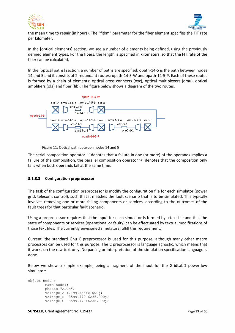
SUNSEED, Grant agreement No. 619437 Page 39 of 66
the mean time to repair (in hours). The “fitkm” parameter for the fiber element specifies the FIT rate per kilometer. In the [optical elements] section, we see a number of elements being defined, using the previously defined element types. For the fibers, the length is specified in kilometers, so that the FIT rate of the fiber can be calculated. In the [optical paths] section, a number of paths are specified. opath-14-5 is the path between nodes 14 and 5 and it consists of 2 redundant routes: opath-14-5-W and opath-14-5-P. Each of these routes is formed by a chain of elements: optical cross connects (oxc), optical multiplexers (omu), optical amplifiers (ola) and fiber (fib). The figure below shows a diagram of the two routes.
Figure 11: Optical path between nodes 14 and 5
The serial composition operator ‘.’ denotes that a failure in one (or more) of the operands implies a failure of the composition, the parallel composition operator ‘+’ denotes that the composition only fails when both operands fail at the same time.
3.1.8.3 Configuration preprocessor
The task of the configuration preprocessor is modify the configuration file for each simulator (power grid, telecom, control), such that it matches the fault scenario that is to be simulated. This typically involves removing one or more failing components or services, according to the outcomes of the fault trees for that particular fault scenario. Using a preprocessor requires that the input for each simulator is formed by a text file and that the state of components or services (operational or faulty) can be effectuated by textual modifications of those text files. The currently envisioned simulators fulfill this requirement. Current, the standard Gnu C preprocessor is used for this purpose, although many other macro processors can be used for this purpose. The C preprocessor is language agnostic, which means that it works on the raw text only. No parsing or interpretation of the simulation specification language is done. Below we show a simple example, being a fragment of the input for the GridLabD powerflow simulator: object node {
name node1;
phases "ABCN";
voltage_A +7199.558+0.000j;
voltage_B -3599.779-6235.000j;
voltage_C -3599.779+6235.000j;

SUNSEED, Grant agreement No. 619437 Page 40 of 66
nominal_voltage 7200; // V
}
#ifndef FAIL_OVERHEAD_LINE_NODE1_NODE2
object overhead_line:12 {
phases "ABCN";
from node1;
to node2;
length 2000; // feet
configuration line_configuration:300;
}
#endif
object node {
name node2;
phases "ABCN";
voltage_A +7199.558+0.000j;
voltage_B -3599.779-6235.000j;
voltage_C -3599.779+6235.000j;
nominal_voltage 7200; // V
}
As long as the parameter FAIL_OVERHEAD_LINE_NODE1_NODE2 is not defined, the overhead link between node1 and node2 is operational. When the paramater is defined, for instance because the preprocessor is called as: cpp -DFAIL_OVERHEAD_LINE_NODE1_NODE2
then the overhead line disappears from the configuration and node1 and node2 are not directly connected anymore. Instead of simply removing elements from the configuration, the preprocessor can also be used to replace an element by a different element or an element with different parameters in certain fault scenarios.
3.1.8.4 Power Flow simulation
Many tools are available for solving sets of power-flow equations, commercially as well as open source. For an extensive list, see [Pow15]. For this project, we looked into a number of open source tools: GridLab-D GridLab-D [Cha14] , [gri15] is a power distribution system simulation and analysis tool developed by the U.S. Department of Energy (DOE) at Pacific Northwest National Laboratory (PNNL) under funding for the Office of Electricity in collaboration with industry and academia.
PNNL describes it as follows: “GridLAB-D™ is a flexible simulation environment that can be integrated with a variety of third-party data management and analysis tools. The core of GridLAB-D™ has an advanced algorithm that simultaneously coordinates the state of millions of independent devices, each of which is described by multiple differential equations. The advantages of this algorithm over traditional finite difference-based simulators are: 1) it handles unusual situations much more accurately; 2) it handles widely disparate time scales, ranging from sub-seconds to many years; and 3) it is very easy to integrate with new modules and third-party systems”.
The focus of GridLab-D is on simulating and solving the power flows in the network in the time domain. OpenDSS

SUNSEED, Grant agreement No. 619437 Page 41 of 66
The OpenDSS [Dug13] is an electric power Distribution System Simulator (DSS) for supporting distributed resource integration and grid modernization efforts. It is developed by the Electric Power Research Institute (EPRI). EPRI is a nonprofit organization funded by the electric utility industry, founded and headquartered in Palo Alto, California. EPRI is primarily a US-based organization, but receives international participation. EPRI's area covers different aspects of electric power generation, delivery and its use [EPRI15]. EPRI describes it as follows: “The OpenDSS is a comprehensive electrical power system simulation tool primarly for electric utility power distribution systems. It supports nearly all frequency domain (sinusoidal steady‐state) analyses commonly performed on electric utility power distribution systems. In addition, it supports many new types of analyses that are designed to meet future needs related to smart grid, grid modernization, and renewable energy research. The OpenDSS tool has been used since 1997 in support of various research and consulting projects requiring distribution system analysis. Many of the features found in the program were originally intended to support the analysis of distributed generation interconnected to utility distribution systems and that continues to be a common use. Other features support analysis of such things as energy efficiency in power delivery and harmonic current flow. The OpenDSS is designed to be indefinitely expandable so that it can be easily modified to meet future needs.” MatPower MATPOWER [Zim11] is a package of MATLAB® M-files for solving power flow and optimal power flow problems. It is intended as a simulation tool for researchers and educators that is easy to use and modify. MATPOWER is designed to give the best performance possible while keeping the code simple to understand and modify. It was initially developed as part of the PowerWeb project. MATPOWER was developed by the Power Systems Engineering Research Center (PSERC). Several U.S. universities and industries cooperate in this institute. The lead university is the Arizona State University. Comparison The following table summarizes some of the main differences between the three above-mentioned tools:
GridLab-D OpenDSS MatPower
Transmission grid + + +
Distribution grid + +
Time domain + +
Frequency domain +
Windows + +
Linux + + +
Graphical User Interface +
Language C/C++ Delphi MatLab
In this phase of the project, no definitive choice has been made which tool to use for power flow calculations. Our objective is a modular set of tools that can be adapted to multiple power flow calculation engines. For the moment, however, we will use GridLab-D for initial experiments. The main output of the Power Flow simulation consists of one or multiple simple parameters that are needed to calculate the overall key performance indicator. For instance, to calculate SAIDI (“availability”), the simulator will produce a binary value for each household that indicates if the power delivery service was operational for that household.

SUNSEED, Grant agreement No. 619437 Page 42 of 66
3.1.8.5 Telecommunication simulation
The telecommunication simulation module simulates the data transport from sensors in the distribution grid (mart meters, WAMS etc) to the control layer and from the control layer to the controllable elements in the distribution network (transformer taps, switchable chargers for electrical vehicles etc). In case of a simple telecommunications network, most of the simulation is already done by the fault trees in the scenario generator module. However, there are cases when the functions of the telecommunications network can not be simulated by fault trees only:
Dynamic routing
Capacity is an important constraint In this stage of the project, we will assume that the telecommunication services can be fully simulated by fault trees, so no advanced telecommunication network simulator is needed. The telecommunication services will be modelled by a number of “switches” that are directly controlled by the outcome of the fault trees. See also the figure below.
Figure 12: Trivial network simulator
3.1.8.6 Control simulation
At the time of writing, not much is known yet about the nature of the control layer that is being developed in the SunSeed project. For the moment, we assume that it will be a set of algorithms that take sensor data as input and produce control signals for various elements in the power distribution grid. One application could be voltage control, in which the control layer can change the settings of a voltage regulator, based on voltage measurements from the network. The control module is assumed to be an executable program that takes sensor values as input and produces one or more control settings. The module can be implemented in any language, as long as it follows the input/output conventions.
3.1.8.7 KPI aggregator
The fault scenario generator generates a large number of fault scenario’s, each with an estimated probability. For each fault scenario, the power flow simulator will produce some values that indicate if the power service was available in that scenario. It is the task of the KPI aggregator to combine all these results into a single, overall Key Performance Indicator (KPI).

SUNSEED, Grant agreement No. 619437 Page 43 of 66
In many cases, this means calculating the weighted average of the simulator outcomes, but other aggregation methods may be possible.
N
j
jj SgPGE2
1
)()(
Here E(G) is the expected value of KPI G, Pj is the probability of fault scenario j, g(Sj) is the outcome of the power flow simulator in scenario j.
3.1.9 Experiments with a trivial grid
In order to test the general principle and the tools that implement them, some first experiments were conducted with a very trivial (and unrealistic) power grid. The plan is that once this gives satisfactory results, a more realistic power grid will be simulated, preferably one that is based on or closely resembles one of the SunSeed pilot grids. The trivial test grid is show in Figure 13
Figure 13: Trivial test grid
3.1.9.1 Power grid
The power grid consists of three nodes (Node0, Node1 & Node2) without any functionality of themselves. Node0 is connected to a higher level network and the voltage is fixed at 25kV (swing bus in the power flow simulation). A set of overhead lines with a length of 8.2 km connect Node0 with Node1. At Node1, a constant power load is connected, representing the load from a number of households. Another set of overhead lines with length of 14.6 km connects Node1 with Node2. At Node2, another constant power load is connected. In addition, a local power generator in the form of a wind generator is also connected to Node2. Node1 and Node2 are equipped with voltage measurement devices (simplified WAMS) that can send the current voltages on the three phases to the central control unit. Finally, the wind generator can be switched on and off by the central control unit. The basic idea is that the central control unit can perform some simple form of voltage control, switching on the wind generator if voltages are low and switching it off when voltages are high. We

SUNSEED, Grant agreement No. 619437 Page 44 of 66
do not claim that this is a realistic example, but it serves our purpose as it introduces some form of feedback control. The power grid is based on the well-known “IEEE 13-bus feeder” [17] [18], which is often used as a reference grid in scientific studies. It is clearly a grid that is based on US practices (many overhead lines, nominal voltage of 2400 V etc.), but in order to be comparable with other studies that use this same grid, it was decided not to convert it to more European standards. For the purpose of demonstrating the feasibility of the method, this does not make any difference. Basic grid The test grid is show in Figure 13.
Figure 12: Test grid, based on IEEE 13-bus test feeder
The power grid consists of:
16 nodes, 10 of which have loads attached to them. Compared to the original 13-node grid, 2 nodes (6321 and 6711) were added to represented the distributed load between nodes 632 and 671 and one node (630) was added for technical reasons between regulator Reg1 and Node 632.
11 power lines connecting the nodes. Most are overhead lines, with the exception of two underground lines feeding nodes 652 and 675. The distances are shown in the figure in feet, the nominal voltage is 2401 V. The phases are indicated by “ABCN”, “CN” etc.
a mixture of constant power (“CP”), constant current (“CC”) and constant impedance (“CI”) loads
two shunt capacitors at nodes 611 and 675
a voltage regulator (Reg1), which can vary the voltages of the three phases independently by +/- 10% in 32 steps.
A transformer that feeds node 634 with 277 V.

SUNSEED, Grant agreement No. 619437 Page 45 of 66
The switch in the original grid (between nodes 671 and 692) has been replaced by 1 feet of overhead line. To give an idea of the level of detail of the GridlabD simulation, we show here the definitions for one overhead line:
// Phase Conductor 1/0 ACSR
object overhead_line_conductor {
name conductor3;
geometric_mean_radius 0.004460;
resistance 1.120000;
}
// ID-505 bcn
object line_spacing {
name line_spacing3;
distance_AC 0.0;
distance_AB 0.0;
distance_BC 7.0;
distance_AN 0.0;
distance_CN 5.656854;
distance_BN 5.0;
}
// Configuration 603
object line_configuration {
name line_configuration3;
conductor_B conductor3;
conductor_C conductor3;
conductor_N conductor3;
spacing line_spacing3;
}
object overhead_line {
name overhead_line1;
phases "BCN";
from Node632;
to Load645;
length 500;
configuration line_configuration3;
}
One example of a load (incl shunt capacitors):
object load {
name Load675;
phases "ABC";
voltage_A 2401.7771;
voltage_B -1200.8886-2080.000j;
voltage_C -1200.8886+2080.000j;
constant_power_A 485000+190000j;
constant_power_B 68000+60000j;
constant_power_C 290000+212000j;
constant_impedance_A 0.00-28.8427j; //Shunt Capacitors
constant_impedance_B 0.00-28.8427j;
constant_impedance_C 0.00-28.8427j;
nominal_voltage 2401.7771;
}
Modelling failures For modelling failures, we use the built-in preprocessor of GridlabD to selectively remove components from the grid. Example: #ifndef overhead_line1_fail
object overhead_line {
name overhead_line1;
phases "BCN";
from Node632;

SUNSEED, Grant agreement No. 619437 Page 46 of 66
to Load645;
length 500;
configuration line_configuration3;
}
#endif
When the global variable “overhead_line1_fail” is defined, overhead line 1 is removed from the network. Defining such variable can be done on the command line by running the simulator as follows:
gridlabd –D overhead_line1_fail=1 ...
For the moment, we assume that lines are either fully operational or completely interrupted. Failures in single phases are not modelled, although they can be added without much effort later. Other faults, like short circuits, are not modelled at this moment. Parametrization of loads For parameterizing quantities like loads, we again use global variables: object load {
name Load671;
phases "ABCD";
voltage_A 2401.7771;
voltage_B -1200.8886-2080.000j;
voltage_C -1200.8886+2080.000j;
constant_power_A_real (385000*${lmf});
constant_power_A_reac (220000*${lmf});
constant_power_B_real (385000*${lmf});
constant_power_B_reac (220000*${lmf});
constant_power_C_real (385000*${lmf});
constant_power_C_reac (220000*${lmf});
nominal_voltage 2401.7771;
}
Here we use the global variable “lmf” (load multiplication factor) to modify the magnitude of a load. Again, this variable can be set on the command line:
gridlabd –D lmf=1.2 ...
We use this parametrization to evaluate each fault scenario’s with 3 different loads. For simplicity, we only vary the load (0.5, 1.0 and 1.5 times the nominal value) of a single node (671) to demonstrate the principle, but for real applications, one may want to simulate many more load scenario’s Voltage sensors We use the built-in mechanism of GridlabD to dump the (complex) voltages of all nodes once the power-flow calculations have converged. This can be interpreted as if every node and load is equipped with voltage measuring WAMS nodes. Other quantities can be measured too, like currents and phases, but these are not used at the moment. A (partial) sample of sensor outputs are show below: Node633:2392.853577,-104.884327,-1241.309331,-2034.487001,-1136.919106,2142.871190
Node630:2495.352831,0.000000,-1200.888600,-2080.000000,-1264.093263,2189.473684
Node632:2400.463698,-102.495026,-1241.998423,-2039.766149,-1139.960347,2148.283112
Node650:2401.777100,0.000000,-1200.888600,-2080.000000,-1200.888600,2080.000000
Node680:2324.410940,-211.503899,-1275.725308,-2052.796543,-1036.685950,2104.717907
Node684:2319.852634,-211.869775,0.000000,0.000000,-1030.414178,2102.658652
Problems with islanding

SUNSEED, Grant agreement No. 619437 Page 47 of 66
GridlabD turned out to have some serious issues with grids in which isolated islands occur. This can easily happen due to the failure of one or more power links. GridlabD offers two different power flow solvers: (1) Newton-Raphson (NR) and (2) Forward-Backward Sweep (FBS). In case on an island, the NR solver detects a singularity and aborts the calculations. The FBW solver continues the calculation, but in each island, one new swing bus is silently introduced at an arbitrary(?) node. Both methods produce undesirable results: the NR solver doesn’t give any solution and the FBS solver produces results that are totally incorrect for the islanded parts. In order to solve this in a quick-and-dirty way, we introduced a small post-processing step on the sensor outputs that sets the sensor values for islanded nodes to zero. A node is islanded if the feeding path from the power source to the node is somewhere interrupted by a failure. Since all the failures are specified in the fault scenario, this is relatively easy to accomplish. One small code fragment of the post processor illustrates this: if( $name=="Load645" ) {
if( defined('overhead_line3_fail') ) $value = $zero;
if( defined('overhead_line1_fail') ) $value = $zero;
}
This is certainly not a desirable solution: when more power sources are involved and/or when a (partly) meshed network is used, it is not so easy to tell when a node becomes islanded. In a later stage, we may switch to a different power flow solver that handles islands in a more elegant way. Controls The only controllable device in the network is voltage regulator Reg1. The tap positions for the three phases are set by global variables, which can be set on the command line. object regulator_configuration {
name regulator_configuration1;
connect_type WYE_WYE;
band_center 2400;
band_width 20.0;
time_delay 30.0;
raise_taps 16;
lower_taps 16;
regulation 0.20;
Control MANUAL;
tap_pos_A `{Reg1A}`;
tap_pos_B `{Reg1B}`;
tap_pos_C `{Reg1C}`;
Setting the tap positions on the command line can be done as follows:
gridlabd –D Reg1A=2 –D Reg1B=0 –D Reg1C=3 ...
Externally to gridlabd, we added the current tap positions to the sensor output, so that the central control unit can read them (provided that the required network links are operational). The only controllable device in the network is voltage regulator Reg1. The tap positions for the three phases are set by global variables, which can be set on the command line. object regulator_configuration {
name regulator_configuration1;
connect_type WYE_WYE;
band_center 2400;
band_width 20.0;
time_delay 30.0;
raise_taps 16;
lower_taps 16;

SUNSEED, Grant agreement No. 619437 Page 48 of 66
regulation 0.20;
Control MANUAL;
tap_pos_A `{Reg1A}`;
tap_pos_B `{Reg1B}`;
tap_pos_C `{Reg1C}`;
Setting the tap positions on the command line can be done as follows:
gridlabd –D Reg1A=2 –D Reg1B=0 –D Reg1C=3 ...
Externally to gridlabd, we added the current tap positions to the sensor output, so that the central control unit can read them (provided that the required network links are operational).
3.1.9.2 Telecommunication network
The telecommunication network is responsible for transporting the sensor values from the power grid to the central control unit in one direction and regulator settings from the central control unit to the power grid in the other direction. For the sake of simplicity, it is modelled by a number of (underground) optic fiber access links (one for each sensor), two aggregating access switches and two optic fiber core links. See Figure .
Figure 13: telecommunication network
The lengths of all (access and core) links are assumed to be 2 km. The two access switches (As01 and As02) roughly serve the “west” (green) and “east” (blue) part of the network. The model only represents the reliability aspects of the telecommunications network. Capacity, delay and other QoS properties are not modelled. The network is simulated by a simple script that can remove one or more sensors from the set of sensor measurements, controlled by command line options. Regulator settings are treated in the same way (in both directions).
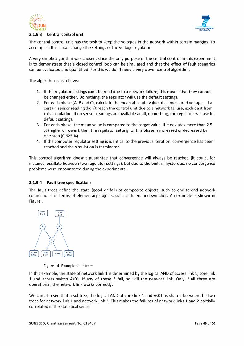
SUNSEED, Grant agreement No. 619437 Page 49 of 66
3.1.9.3 Central control unit
The central control unit has the task to keep the voltages in the network within certain margins. To accomplish this, it can change the settings of the voltage regulator. A very simple algorithm was chosen, since the only purpose of the central control in this experiment is to demonstrate that a closed control loop can be simulated and that the effect of fault scenarios can be evaluated and quantified. For this we don’t need a very clever control algorithm. The algorithm is as follows:
1. If the regulator settings can’t be read due to a network failure, this means that they cannot be changed either. Do nothing, the regulator will use the default settings.
2. For each phase (A, B and C), calculate the mean absolute value of all measured voltages. If a certain sensor reading didn’t reach the control unit due to a network failure, exclude it from this calculation. If no sensor readings are available at all, do nothing, the regulator will use its default settings.
3. For each phase, the mean value is compared to the target value. If it deviates more than 2.5 % (higher or lower), then the regulator setting for this phase is increased or decreased by one step (0.625 %).
4. If the computer regulator setting is identical to the previous iteration, convergence has been reached and the simulation is terminated.
This control algorithm doesn’t guarantee that convergence will always be reached (it could, for instance, oscillate between two regulator settings), but due to the built-in hysteresis, no convergence problems were encountered during the experiments.
3.1.9.4 Fault tree specifications
The fault trees define the state (good or fail) of composite objects, such as end-to-end network connections, in terms of elementary objects, such as fibers and switches. An example is shown in Figure .
Figure 14: Example fault trees
In this example, the state of network link 1 is determined by the logical AND of access link 1, core link 1 and access switch As01. If any of these 3 fail, so will the network link. Only if all three are operational, the network link works correctly. We can also see that a subtree, the logical AND of core link 1 and As01, is shared between the two trees for network link 1 and network link 2. This makes the failures of network links 1 and 2 partially correlated in the statistical sense.

SUNSEED, Grant agreement No. 619437 Page 50 of 66
First we define the failure properties of the elementary object types: # fitrate = number of failures in 10^9 hours
overhead_line = elem fitkm=2282 mttr=24; [ mtbf=1 yr per 50 km]
underground_line= elem fitkm=1141 mttr=24; [ mtbf=1 yr per 100 km]
fiber = elem fitkm=1141 mttr=24; [ mtbf=1 yr per 100 km]
switch = elem fit=57077 mttr=4; [ mtbf=2 yr]
controller = elem fit=57077 mttr=4; [ mtbf=2 yr]
These type definitions define the failure (FIT) rates and mean time to repair (MTTR) values. For cables, wires and optical fibers, the failure rates are specified per km. We assume the failure rates of optical fiber and underground power lines are once per year per 100 km, a common value used in telecommunications for underground cables. For overhead wires, we assume once per year per 50 km. Network switches and the central controller are assumed to fail once per 2 years on average. All these values are arbitrary and may not reflect the real values in practice, but for the moment they suffice to demonstrate the general principle. The actual elementary object are then defined in terms of generic object types above: overhead1: overhead_line km=0.1524; [ 500ft ]
overhead2: overhead_line km=0.09144; [ 300ft ]
access_link1: fiber km=2;
access_link2: fiber km=2;
Here the actual length of the lines is specified and this is used to calculate the actual failure rate. Finally, the fault trees are specified by means of Boolean expressions: overhead_line1: tree global value=( overhead1 );
overhead_line2: tree global value=( overhead2 );
network_link1: tree global value=( access_link1 . As01 . core_link1 );
network_link2: tree global value=( access_link2 . As01 . core_link1 ); The fact that the trees for network_link1 and network_link2 share a common subtree is not explicitly specified, but this is automatically discovered by the software. These fault trees are used to generate a set of fault scenarios, sorted to ascending probability. Here are the first 8: : 9.982349309742e-01
network_link1 network_link2 network_link3 network_link4
network_link5 network_link6 network_link7 network_link8
network_link16 : 2.827281246496e-04
network_link9 network_link10 network_link11 network_link12
network_link13 network_link14 network_link15 : 2.826971709991e-04
Control : 2.279050206209e-04
network_link9 : 5.467133069960e-05
network_link8 : 5.467133069960e-05
network_link7 : 5.467133069960e-05
network_link6 : 5.467133069960e-05
Each line defines a single fault scenario and contains the set of failing elements, a colon and the probability. The first line defines the scenario without any failures. This scenario has a probability of 99.8%.

SUNSEED, Grant agreement No. 619437 Page 51 of 66
The second line defines a scenario in which many network links are interrupted at the same time, probably because of a failing access switch or a core link. The subsequent lines each define a scenario with a single end-to-end network failure (caused by failing access links) For most experiments, a set of 50 fault scenarios was generated that together cover 99.9999% of the total state space. The uncertainly in reliability outcomes is therefore equal to 0.0001% (1.10-6), in general enough to calculate values in the range of “5 nines” (99.999%)
3.1.9.5 Powergrid specification
The text below specifies the power grid network for the purpose of power flow simulations with the GridLabD program. // specifications of wires ommitted
// nodes
object node {
name Node0;
bustype SWING;
phases ABC;
nominal_voltage 25000.0 V;
}
object node {
name Node1;
phases ABC;
nominal_voltage 25000.0 V;
}
object node {
name Node2;
phases ABC;
nominal_voltage 25000.0 V;
}
// electrical lines
object overhead_line {
name Link1;
phases A|B|C;
from Node0;
to Node1;
length 8200 m;
configuration LC300;
nominal_voltage 25000.0 V;
status CLOSED;
}
object overhead_line {
name Link2;
phases A|B|C;
from Node1;
to Node2;
length 24600 m;
configuration LC300;
nominal_voltage 25000.0 V;
status CLOSED;
}
// loads
object load {
name Load1;
phases ABC;
parent Node1;
object player {
property constant_power_A; // default unit = VA
file loadA1.csv;
};
object player {
property constant_power_B;
file loadB1.csv;

SUNSEED, Grant agreement No. 619437 Page 52 of 66
};
object player {
property constant_power_C;
file loadC1.csv;
};
nominal_voltage 25000.0 V;
}
object load {
name Load2;
parent Node2;
phases ABC;
object player {
property constant_power_A;
file loadA2.csv;
};
object player {
property constant_power_B;
file loadB2.csv;
};
object player {
property constant_power_C;
file loadC2.csv;
};
nominal_voltage 25000.0 V;
}
// wind generation
object load {
name Wind;
parent Node2;
phases ABC;
object player {
property constant_power_A;
file windA.csv;
};
object player {
property constant_power_B;
file windB.csv;
};
object player {
property constant_power_C;
file windC.csv;
};
nominal_voltage 25000.0 V;
}
// recorders
object recorder {
name VoltageNode1;
parent Node1;
property voltage_A,voltage_B,voltage_C;
file voltage1.csv;
}
object recorder {
name VoltageNode2;
parent Node2;
property voltage_A,voltage_B,voltage_C;
file voltage2.csv;
}
3.1.9.6 Results
Uncertainty The first thing we investigated is how quickly the uncertainty in outcomes becomes small enough to be of practical value. Remember that we only generate and evaluate an incomplete set of fault scenarios, hopefully containing the most prominent ones. We do not know what the outcome would be for the fault scenarios that we do not generate and evaluate, so the sum of the probabilities of these unevaluated scenarios forms the uncertainty. This sum is equal to one minus the probability of the scenario’s we do evaluate, so we can easily calculate how large or small that uncertainty is. The graph in Figure 14 shows the uncertainty as function of the number of generated fault scenarios (note the logarithmic vertical axis):

SUNSEED, Grant agreement No. 619437 Page 53 of 66
Figure 14: Uncertainty as function of number of fault scenario's
Initially, the uncertainty is quite large, but drops quickly. From 32 fault scenario’s onward, the speed of decrease becomes lower as the probability of individual fault scenario’s suddenly becomes so small that evaluating them does not decrease the uncertainty as much as before. This corresponds with the point where the fault scenario generator switches from generating individual faults to combinations of 2 faults (which have much lower probability). If we go much further in generating fault scenario’s, the uncertainty keeps decreasing, as shown in Figure 15.
Figure 15: Uncertainty as function of number of fault scenario's
We can clearly see the points were the fault scenario generator switches from 1 to 2 to 3 simultaneous faults. We also see that an uncertainty of 10-12 can be reached, at the expense of generating and evaluating roughly 4000 fault scenario’s. Obviously, solving the power flow in 4000 fault scenario’s is going to be computationally intensive, and in this particular case, this would be a waste of resources. For the rest of the experiments, we limited the number of fault scenarios to 50. For every fault scenario, we simulate 3 different load scenario’s, so in the graphs that follow, the number of scenarios run from 1 to 150. Passive mode (no voltage control)
1 fault
2 faults
3 faults

SUNSEED, Grant agreement No. 619437 Page 54 of 66
In passive mode, the voltage control by the central control unit is disabled and the telecommunication network links are not used. The voltage regulator is set to its default setting, which was chosen to give the best results for the grid in absence of any faults. Figure 16 shows the results for Load692, phase B in passive mode.
Figure 16: Load692, phase B, passive mode
The horizontal axis shows the number of fault scenario’s. Remember that for each “real” fault scenario, we run 3 different load scenario’s, so in total, we evaluated 50×3 fault scenario’s The vertical axis shows the probabilities of power outage (green), under voltage (blue) and overvoltage (red). The crosshatched areas represent the uncertainty in the outcome for these three measures, which means that the “real” value is somewhere located in the filled area. Most useful is the upper bound to these quantities that decreases when the number of scenario’s increases. The green crosshatched area gives the outage probability. In this experiment, outage is only caused by broken power lines. We can see that after roughly 100 scenario’s, the difference between the upper and lower bound becomes so small that evaluating more scenario’s won’t increase the accuracy. The real value must be between 3.67.10-5 and 3.77.10-5, which means an availability of 99.996%. The blue crosshatched area represents the probability of under voltage (more than 5% below the nominal voltage). This is most likely caused by the varying loads. Apparently, in a few fault scenario’s the default regulator settings is not optimal. After evaluating approx. 90 scenario’s, there is still some margin between the upper and lower bounds, which only slowly decreases when evaluating more scenario’s. The real value must be between 1.39.10-6 and 2.42.10-6. During the simulation, we did not encounter any scenario’s that result in overvoltage. Here the upper bound is equal to the uncertainty (the total probability of all fault scenario’s that we did not evaluate), the same as shown in Figure 14. The lower bound is obviously equal to zero. Active mode

SUNSEED, Grant agreement No. 619437 Page 55 of 66
In active mode, voltage control is enabled. As described before, the central control unit tries to keep the average absolute value of all measured voltages for each phase within certain bounds. It does this by reading the sensors at each of the nodes and changing the regulator settings if needed. This results in the following graph:
Figure 17: Load692, phase B, active mode
We see here that the under voltage disappeared as a result of the voltage control. The outage probability did not change as voltage control has no influence on it: it is purely the results of power line outages. The very simple and “naïve” voltage control algorithm does not always lead to the desired result, as can be seen from the graphs in Figure 18 and Figure 19.
Figure 18: Load611, phase C, passive mode

SUNSEED, Grant agreement No. 619437 Page 56 of 66
Figure 19: Load611, phase C, active mode
Although the voltage control works correctly in the case of no faults, in certain fault scenario’s it actually introduces under voltage that wasn’t there in the passive case. Clearly, the control algorithm is not as smart as we would wish: by controlling the mean value of all voltages of a certain phase, it doesn’t pay attention to individual voltages that exceed the allowed thresholds. An alternative control strategy could be to minimize the number of individual voltages that exceed the allowed tolerance, but this hasn’t been implemented yet. This last example nicely demonstrates the benefits of having a method to evaluate the performance of a SmartGrid in various fault scenario’s. The control algorithm we implemented looked good at first sight as it works correctly in the case of no faults in the system. However, in certain fault scenario’s, the control algorithm becomes counterproductive as it results in a performance that is even worse than the case without voltage control. Such observations are extremely valuable feedback to the design of the SmartGrid, especially to the design of the control algorithm and possibly the implementation of the telecommunication network. As an example of the last: we may find that it is wiser to connect the access links in a more random fashion to the two access switches, so that the control unit does not become completely “blind” for one part of the network in case of a core switch or core link failure.
3.1.10 Conclusions and plans for further work
3.1.10.1 Conclusions
Since this report describes work in progress, no final conclusions can be drawn about the feasibility of estimating availability and other KPIs of smart grids by means of the proposed method. However, a few remarks can be made that follow from the work so far. The transition from a classical, passive distribution grid to an active, “smart” grid usually implies the addition of various telecommunications and IT components. This can have a significant impact on the performance and stability of the grid, but it is not easy to say if this will be positive or negative. More components means more failures, but smart control strategies can also limit the impact of failures, for instance by fault isolation or by power rerouting. Careful analysis, for instance by simulations,

SUNSEED, Grant agreement No. 619437 Page 57 of 66
should be performed to assure that the performance of the grid will not be degraded by the transition. A grid in which sensors, controlable (power) components, telecommunication links and control nodes work together can be viewed as a dynamic system with one or more feedback loops (in the sense of the classical control theory). For predicting the behaviour of such systems, one has to study the system as a whole, including the closed feedback loop(s). One can not predict the behaviour, including the expected performance, by studying individual sub systems (power grid, telecommunications network, control algorithms) since this ignores the closed-loop nature. Except for trivial designs, it is hard to evaluate the performance of the complete system when being affected by (random) failures without looking into the different failure scenarios individually. Each failure scenario (combination of one or more failures) may cause a different response from the feedback system and may have a different outcome for the performance. The proposed method is based on the systematic simulation of a large number (but not all) of those failure scenarios, up to the point where sufficient accuracy has been reached. The basic principle of this method has been used before succesfully for the evaluation of the performance of large telecommunications core networks. A number of candidate power flow analysis tools (GridlabD, OpenDSS, MatPower) have been identified for these simulations. Some experiments with GridlabD have shown that it is possible to integrate this tool into an evaluation system that implements the described method of systematic but incomplete failure scenario simulations. The experiments that have been carried out demonstrated the benefits of having a method to evaluate the performance of a SmartGrid in various fault scenario’s. The control algorithm we implemented looked good at first sight as it works correctly in the case of no faults in the system. However, in certain fault scenario’s, the control algorithm becomes counterproductive as it results in a performance that is even worse than the case without voltage control. Such observations are valuable feedback to the design of the SmartGrid. An important question that has not been answered yet is whether the proposed method is scalable enough to handle the complexity and number of components of a typical “smart” distribution grid, such that sufficient accuracy can be reached within reasonable computation time.
3.1.10.2 Plans for further work
In case sufficient details become available about the grids that will be used for the SunSeed field tests, these could be used for more realistic experiments with the proof-of-concept tool. The current version of the proof-of-concept tool only calculates availability ratio’s (SAIDI). In previous (internal) research, it has been shown that the fault scenario generation algorithm and the KPI aggregator can be extended in such a way that they can also produce values for interruption frequency (SAIFI) and interruption duration (CAIDI). Another possible extension is that components can be tagged by the number of customers that they serve. This makes it possible to simulate a network that contains different hierarchy levels, without necessarily including all the customers that are served by the highest level. It also allows to assign a “severity” attribute to interruptions, indicating how many customers are affected by it. That makes it

SUNSEED, Grant agreement No. 619437 Page 58 of 66
possible to quantify, for instance, the expected number of interruption per year that affect 1000 customers or more.
3.2 SG data collection
3.2.1 Data storage/message format
Data is the fundamental substance of the smart grid. Thus, a clear understanding of how this data is obtained, what it consists of and the benefits it can be used to deliver is critical to realizing the fullest possible returns from smart grid investments. In terms of the flow of smart grid data, there are different architectural stages that can be used to guide the design of the data management structure [D2.2.1]. We can describe them using the following steps:
1. Data is initially generated by network devices such as smart meters (e.g. AMI), grid measurement (e.g. CP-SPM and CP-PMC nodes) and control nodes, and also generated by other data sources (e.g. weather forecast).
2. Data is transported for storage and processing by various applications using different communication technologies (e.g. LTE, power line).
3. Within the different modules/applications/platforms raw measurement data are processed and used as an input for further calculations (e.g. state estimation, load forecasting, etc.). The results are then further processed in additional modules/applications for real and non-real time operations either used directly by automated systems or for visualisation purposes.
4. Information must be presented to people in forms they can easily understand through different visualizations so the appropriate actions can be taken.
The message content and data storage can be encoded in one of many binary and text formats. Binary formats advances from efficient serialization and de-serialization of data and their compactness, but lack of human readability makes debugging and diagnosing problems more difficult. Moreover, many native libraries provide strong support for text-based encoding like XML (Extensible Markup Language) or JSON (JavaScript Object Notation). JSON, at first mostly used in web-based applications due to easy conversion to/from JavaScript objects, is becoming increasingly popular due its simplicity and compactness. As it is native programming entity in case of Javascript server engines like Node.js, JSON is suitable and eases agile software development, as also elaborated in deliverable D4.1.1 [D4.1.1]. Thus, for the message format we selected JSON, which has different advantages. It is a lightweight data-interchange format and is easy for humans to read and write. It is easy for machines to parse and generate. JSON is a text format that is completely language independent but uses conventions that are familiar to programmers of the C-family of languages, used for modules development also within SUNSEED, including C, C++, C#, Java, JavaScript, Perl, Python, and many others. These properties make JSON an ideal data-interchange format. In addition MongoDB, selected as NoSQL database for SUNSEED, also stores data in JSON like documents. JSON is built on two structures [JSON]:
A collection of name/value pairs. In various languages, this is realized as an object, record, struct, dictionary, hash table, keyed list, or associative array.
An ordered list of values. In most languages, this is realized as an array, vector, list, or sequence.
These are universal data structures. Virtually all modern programming languages support them in one form or another. It makes sense that a data format that is interchangeable with programming languages also be based on these structures.

SUNSEED, Grant agreement No. 619437 Page 59 of 66
The data can be divided into two main groups namely the data measurement, used as input for further calculations, and derived data as presented in Figure 20.
AMI measurements
SPM measurements
PMC measurements
SE data
P/Q data
Forecasting data
MongoDB
SE Calculation
P/Q data Calculation
Load Forecasting Calculation
SQL
JSON structure
DSOtopology data
other data sourceseg. weather
Figure 20: Data structure.
In the following we present the JSON fields of each data group. All values are in double precision, except node_id which is integer and time stamps, which are in UNIX date format. The data can be categorized as we discussed in deliverable D2.2.1 [D2.2.1] also according to different time scales (e.g. from seconds to days). The updating frequency of the AMI measurements is approximately 15 minutes, while for SPM and PMC measurements the updating frequency is 1 s. Based on the above the SE and power flow data is calculated on 1s, while forecasting is done on 15 minutes bases.

SUNSEED, Grant agreement No. 619437 Page 60 of 66
Parent Name Type Description
am
i
node_id array Unique node identification
v1 array Voltage magnitude for phase 1
v2 array Voltage magnitude for phase 2
v3 array Voltage magnitude for phase 3
i1 array Current magnitude for phase 1
i2 array Current magnitude for phase 2
i3 array Current magnitude for phase 3
i4 array Current magnitude for neutral
f1 array Frequency
p1 array Active power for phase 1
p2 array Active power for phase 2
p3 array Active power for phase 3
q1 array Reactive power for phase 1
q2 array Reactive power for phase 2
q3 array Reactive power for phase 3
vv1 array Voltage violation for phase 1
vv2 array Voltage violation for phase 2
vv3 array Voltage violation for phase 3
stamp array Measurement time stamp in UNIX date format
Table 7: AMI measurement JSON structure.

SUNSEED, Grant agreement No. 619437 Page 61 of 66
Parent Name Type Description
pm
u
node_id array Unique node identification
v1 array Voltage magnitude for phase 1
v2 array Voltage magnitude for phase 2
v3 array Voltage magnitude for phase 3
th1 array Phase angle 1
th2 array Phase angle 2
th3 array Phase angle 3
psp_v array Positive sequence voltage magnitude
psp_th array Positive sequence phase angle
status array PMU status flags
f1 array Frequency for phase 1
f2 array Frequency for phase 2
f3 array Frequency for phase 3
f4 array Frequency for positive sequence phasor
df1 array Rate of change of frequency for phase 1
df2 array Rate of change of frequency for phase 2
df3 array Rate of change of frequency for phase 3
df4 array Rate of change of freq. for positive sequence phasor
stamp1 array Measurement time stamp in UNIX date format
stamp2 array Measurement time stamp in UNIX date format
Table 8: SPM measurement JSON structure.

SUNSEED, Grant agreement No. 619437 Page 62 of 66
Parent Name Type Description
pm
c
node_id array Unique node identification
v1 array Voltage magnitude for phase 1
v2 array Voltage magnitude for phase 2
v3 array Voltage magnitude for phase 3
i1 array Current magnitude for phase 1
i2 array Current magnitude for phase 2
i3 array Current magnitude for phase 3
i4 array Current magnitude for neutral
f1 array Frequency
p1 array Active power for phase 1
p2 array Active power for phase 2
p3 array Active power for phase 3
q1 array Reactive power for phase 1
q2 array Reactive power for phase 2
q3 array Reactive power for phase 3
stamp array Measurement time stamp in UNIX date format
Table 9: PMC measurement JSON structure.
Parent Name Type Description
se
node_id array Unique node identification
v1 array Voltage magnitude for phase 1
v2 array Voltage magnitude for phase 2
v3 array Voltage magnitude for phase 3
th1 array Phase angle 1
th2 array Phase angle 2
th3 array Phase angle 3
timestamp array Measurement time stamp in UNIX date format
Table 10: SE d JSON structure.

SUNSEED, Grant agreement No. 619437 Page 63 of 66
Parent Name Type Description
pq
node_id array Unique node identification
p1i array Active injection power for phase 1
p2i array Active injection power for phase 2
p3i array Active injection power for phase 3
q1i array Reactive injection power for phase 1
q2i array Reactive injection power for phase 2
q3i array Reactive injection power for phase 3
p1mss array Active power for phase 1 (from MSS)
p2mss array Active power for phase 2 (from MSS)
p3mss array Active power for phase 3 (from MSS)
q1mss array Reactive power for phase 1 (from MSS)
q2mss array Reactive power for phase 2 (from MSS)
q3mss array Reactive power for phase 3 (from MSS)
stamp array Measurement time stamp in UNIX date format
Table 11: P/Q data JSON structure.
Parent Name Type Description
stlf
node_id array Unique node identification
p1i array Forecasted Active injection power for phase 1
p2i array Forecasted Active injection power for phase 2
p3i array Forecasted Active injection power for phase 3
q1i array Forecasted Reactive injection power for phase 1
q2i array Forecasted Reactive injection power for phase 2
q3i array Forecasted Reactive injection power for phase 3
p1mss array Forecasted Active power for phase 1 (from MSS)
p2mss array Forecasted Active power for phase 2 (from MSS)
p3mss array Forecasted Active power for phase 3 (from MSS)
q1mss array Forecasted Reactive power for phase 1 (from MSS)
q2mss array Forecasted Reactive power for phase 2 (from MSS)
q3mss array Forecasted Reactive power for phase 3 (from MSS)
stampm array Measurement time stamp in UNIX date format
stampf array Forecasted time stamp in UNIX date format
Table 12: Short term load forecasting JSON structure.
An example of two SPM measurement, retrieved from the database, for two different nodes at the same time is presented in Figure 21.. It is worth noting that the measurement message from one WAMS-SPM device will have only one entry in the array.

SUNSEED, Grant agreement No. 619437 Page 64 of 66
{"_id":{"$oid":"56168d55ac205804c70d7899"},"df1":[0,0],"df2":[0,0],"df3":[0,0],
"df4":[0,0],
"f1":[50,50],"f2":[50,50],"f3":[50,50],"f4":[50,50],"node_id":[12041710,1406251
8],
"psp_th": [0.00892984499],"psp_v":[0.998195486,0.9990399247],
"stamp1":[1444311338,1444311338],"stamp2":[1444311338,1444311338],"status":[0,0
],
"th1":[7.8e-05,-0.008810845],"th2":[0.000148,-0.0087478449999],
"th3":[0.000158,-0.008698844],"v1":[0.9962754861,0.99748992],
"v2":[0.9977254861,0.9971299247],"v3":[0.9966254861,0.99850992]}
Figure 21: An example of JSON structure for two nodes SPM data.

SUNSEED, Grant agreement No. 619437 Page 65 of 66
4 References
[Cen94] CENELEC, " Voltage characteristics of electricity supplied by public distribution systems," CENELEC, 1994.
[Cha14] D. P. Chassin, J. C. Fuller and N. Djilali, "GridLAB-D: An agent-based simulation framework for smart grid," Journal of Applied Mathematics, 2014.
[Cia09] E. Ciapessoni, D. Cirio and al., "A Probabilistic Risk Assessment Approach to support the operation of large power systems," in Proceedings of the IEEE Power Systems Conference and Exposition, Seattle USA, 2009.
[Cia10] E. Ciapessoni, D. Cirio and al., "Operational Risk Assesment and Control: a probabilistic approach," in Innovative Smart Grid Technologies Conference Europe, 2010.
[D2.2.1] Preliminary specification of SUNSEED field trial requirements for communication, metering, data collection, SUNSEED Deliverable report, 2015.
[D4.1.1] DSO Grid Model description, SUNSEED Deliverable report, 2015. [Dug13] R. C. Dugan, "The Open Distribution System Simulator Reference Guide," 2013. [Dup10] B. Dupont, L. Meeus and R. Belman, "Measuring the 'Smartness'of the Electricity Grid,"
in Proceedings of the 2010 7th International Conference on the European Energy Market (EEM), Madrid, 2010.
[EPRI15] EPRI. [Online]. Available: http://www.epri.com. [Accessed July 2015]. [Galv 2011] Electricity reliability: Progress, problems and policy solutions, Galvin Electricity
Initiative, 2011. [gpx15] gpx.nl. [Online]. Available: http://www.gpx.nl/gpx/grid.htm. [Accessed July 2015]. [Gra06] J. Grainger and W. Stevenson, Power System Analysis, New York: Mc-Graw-Hill, 1994. [gri15] gridlabd.org, "GridLAB-D," [Online]. Available: http://www.gridlabd.org/. [Accessed July
2015]. [Harr02] Harrington, David, Bert Wijnen, and Randy Presuhn. "An architecture for describing
simple network management protocol (SNMP) management frameworks." (2002). [Her06] D. V. Hertem, J. Verboomen, K. Purchala and R. Belmans, "Usefulness of DC Power Flow
for Active Power Flow Analysis with Flow Controlling Devices," in ACDC 2006, The 8th IEE International Conference on AC and DC Power Transmission, 2006.
[Hoo15] Hoogspanningsnet.com, "De netkaart van Nederland en België in Google Earth," [Online]. Available: http://www.hoogspanningsnet.com/google-earth/standaardnetkaart/. [Accessed July 2015].
[IEC61850] IEC 61850-5: Communication networks and systems for power utility automation – Part 5: Communication requirements for functions and device models
[IEEE 2012] IEEE Guide for Electric Power Distribution Reliability Indices, IEEE 1366-2012, 2012. [IEEE11] IEEE, "1366-2012 - IEEE Guide for Electric Power Distribution Reliability Indices," IEEE. [JSON] http://www.json.org/ , 2016. [Met14] K. Mets, J. Aparicio and C. Develder, "Combining power and communication network
simulation for cost-effective smart grid analysis," IEEE COMMUN. SURVEYS & TUTORIALS – SPECIAL ISSUE ON ENERGY AND SMART GRID, vol. 16, no. 3, pp. 1771-1796, 2014.
[Nel11] D. Nel, "Bulk water distribution power supply failures," J. S. Afr. Inst. Civ. Eng., vol. 53, no. 1, apr 2011.
[NIB15] NIBUD, "Energie en water," [Online]. Available: http://www.nibud.nl/consumenten/energie-en-water/. [Accessed July 2015].
[NIS10] Introduction to NISTIR 7628 Guidelines for Smart Grid Cyber Security, NIST, 2010.

SUNSEED, Grant agreement No. 619437 Page 66 of 66
[Pow15] www.openelectrical.org, "Power Systems Analysis Software," [Online]. Available: http://www.openelectrical.org/wiki/index.php?title=Power_Systems_Analysis_Software. [Accessed July 2015].
[Powe15] "Power Flow Study," [Online]. Available: http://en.wikipedia.org/wiki/Power-flow_study. [Accessed jul 2015].
[PPA 2012] Performance benchmarking for Pacific power utilities, Pacific Power Association, 2012. [Spi15] Wikipedia, "Spijkerkwartier," [Online]. Available:
https://nl.wikipedia.org/wiki/Spijkerkwartier. [Accessed July 2015]. [Uni15] An introduction to the Universal Smart Energy Framework,
https://ec.europa.eu/energy/sites/ener/files/documents/xpert_group3_summary.pdf [Ven12] P. Venemans and M. Schreuder, "A Method for the Quantitative Assesment of Reliability
of Smart Grids," in CIRED Workshop, Lisbon, 2012. [ver15] verbruiken.nl, "Hoeveel elektriciteit verbruik ik per dag?," [Online]. Available:
http://www.verbruiken.nl/blog/Hoeveel-elektriciteit-verbruik-ik-per-dag-20130610. [Accessed July 2015].
[WB 2009] Monitoring Performance of Electric Utilities, World Bank, 2009. [Zim11] R. Zimmerman, C. Murillo-Sanchez and R. Thomas, "MATPOWER: Steady-State
Operations, Planning and Analysis Tools for Power Systems Research and Education," IEEE Transactions on Power Systems, vol. 26, no. 1, pp. 12-19, Feb 2011.