cse 291: advanced techniques in algorithm design · of yuval filmus: yuvalf/. 1.1 strassen’s...
TRANSCRIPT

CSE 291: Advanced techniques in algorithm design
Shachar Lovett
Spring 2016
Abstract
The class will focus on two themes: linear algebra and probability, and their manyapplications in algorithm design. We will cover a number of classical examples, includ-ing: fast matrix multiplication, FFT, error correcting codes, cryptography, efficientdata structures, combinatorial optimization, routing, and more. We assume basic fa-miliarity (undergraduate level) with linear algebra, probability, discrete mathematicsand graph theory.
1

Contents
0 Preface: Mathematical background 40.1 Fields . . . . . . . . . . . . . . . . . . . . . . . . . . . . . . . . . . . . . . . 40.2 Polynomials . . . . . . . . . . . . . . . . . . . . . . . . . . . . . . . . . . . . 40.3 Matrices . . . . . . . . . . . . . . . . . . . . . . . . . . . . . . . . . . . . . . 50.4 Probability . . . . . . . . . . . . . . . . . . . . . . . . . . . . . . . . . . . . 5
1 Matrix multiplication 71.1 Strassen’s algorithm . . . . . . . . . . . . . . . . . . . . . . . . . . . . . . . 71.2 Verifying matrix multiplication . . . . . . . . . . . . . . . . . . . . . . . . . 111.3 Application: checking if a graph contains a triangle . . . . . . . . . . . . . . 121.4 Application: listing all triangles in a graph . . . . . . . . . . . . . . . . . . . 12
2 Fast Fourier Transform and fast polynomial multiplication 142.1 Univariate polynomials . . . . . . . . . . . . . . . . . . . . . . . . . . . . . . 142.2 The Fast Fourier Transform . . . . . . . . . . . . . . . . . . . . . . . . . . . 142.3 Inverse FFT . . . . . . . . . . . . . . . . . . . . . . . . . . . . . . . . . . . . 162.4 Fast polynomial multiplication . . . . . . . . . . . . . . . . . . . . . . . . . . 162.5 Multivariate polynomials . . . . . . . . . . . . . . . . . . . . . . . . . . . . . 17
3 Secret sharing schemes 193.1 Construction of a secret sharing scheme . . . . . . . . . . . . . . . . . . . . . 193.2 Lower bound on the share size . . . . . . . . . . . . . . . . . . . . . . . . . . 21
4 Error correcting codes 234.1 Basic definitions . . . . . . . . . . . . . . . . . . . . . . . . . . . . . . . . . . 234.2 Basic bounds . . . . . . . . . . . . . . . . . . . . . . . . . . . . . . . . . . . 244.3 Existence of asymptotically good codes . . . . . . . . . . . . . . . . . . . . . 254.4 Linear codes . . . . . . . . . . . . . . . . . . . . . . . . . . . . . . . . . . . . 26
5 Reed-Solomon codes 275.1 Definition . . . . . . . . . . . . . . . . . . . . . . . . . . . . . . . . . . . . . 275.2 Decoding Reed-Solomon codes from erasures . . . . . . . . . . . . . . . . . . 285.3 Decoding Reed-Solomon codes from errors . . . . . . . . . . . . . . . . . . . 28
6 Polynomial identity testing and finding perfect matchings in graphs 306.1 Perfect matchings in bi-partite graphs . . . . . . . . . . . . . . . . . . . . . . 306.2 Polynomial representation . . . . . . . . . . . . . . . . . . . . . . . . . . . . 316.3 Polynomial identity testing . . . . . . . . . . . . . . . . . . . . . . . . . . . . 336.4 Perfect matchings via polynomial identity testing . . . . . . . . . . . . . . . 34
2

7 Satisfiability 367.1 2-SAT . . . . . . . . . . . . . . . . . . . . . . . . . . . . . . . . . . . . . . . 367.2 3-SAT . . . . . . . . . . . . . . . . . . . . . . . . . . . . . . . . . . . . . . . 40
8 Hash functions: the power of pairwise independence 428.1 Pairwise independent bits . . . . . . . . . . . . . . . . . . . . . . . . . . . . 428.2 Application: de-randomized MAXCUT . . . . . . . . . . . . . . . . . . . . . 448.3 Optimal sample size for pairwise independent bits . . . . . . . . . . . . . . . 458.4 Hash functions with large ranges . . . . . . . . . . . . . . . . . . . . . . . . 468.5 Application: collision free hashing . . . . . . . . . . . . . . . . . . . . . . . . 478.6 Efficient dictionaries: storing sets efficiently . . . . . . . . . . . . . . . . . . 488.7 Bloom filters . . . . . . . . . . . . . . . . . . . . . . . . . . . . . . . . . . . . 50
9 Min cut 519.1 Karger’s algorithm . . . . . . . . . . . . . . . . . . . . . . . . . . . . . . . . 519.2 Improving the running time . . . . . . . . . . . . . . . . . . . . . . . . . . . 53
10 Routing 5510.1 Deterministic routing is bad . . . . . . . . . . . . . . . . . . . . . . . . . . . 5510.2 Randomized routing saves the day . . . . . . . . . . . . . . . . . . . . . . . . 57
11 Expander graphs 6011.1 Edge expansion . . . . . . . . . . . . . . . . . . . . . . . . . . . . . . . . . . 6011.2 Spectral expansion . . . . . . . . . . . . . . . . . . . . . . . . . . . . . . . . 6111.3 Cheeger inequality . . . . . . . . . . . . . . . . . . . . . . . . . . . . . . . . 6411.4 Random walks mix fast . . . . . . . . . . . . . . . . . . . . . . . . . . . . . . 6511.5 Random walks escape small sets . . . . . . . . . . . . . . . . . . . . . . . . . 6611.6 Randomness efficient error reduction in randomized algorithms . . . . . . . . 68
3

0 Preface: Mathematical background
0.1 Fields
A field is a set F endowed with two operations: addition and multiplication. It satisfies thefollowing conditions:
• Associativity: (x+ y) + z = x+ (y + z) and (xy)z = x(yz).
• Commutativity: x+ y = y + x and xy = yx.
• Distributivity: x(y + z) = xy + xz.
• Unit elements (0,1): x+ 0 = x and x1 = x.
• Inverse: If x 6= 0 then there exists 1/x such that x(1/x) = 1.
You probably know many infinite fields: the real numbers R, the rationals Q and thecomplex numbers C. For us, the most important fields will be finite fields, which have afinite number of elements.
An example is the binary field F2 = 0, 1, where addition corresponds to XOR andmultiplication to AND. This is an instance of a more general example, of prime finite fields.Let p be a prime. The field Fp consists of the elements 0, 1, . . . , p− 1, where addition andmultiplication are defined modulo p. One can verify that it is indeed a field. The followingfact is important, but we will not prove it.
Fact 0.1. If a finite field F has q elements, then q must be a prime power. For any primepower there is exactly one finite field with q elements, which is called the finite field of orderq, and denoted Fq.
0.2 Polynomials
Univariate polynomials over a field F are given by
f(x) =n∑i=0
fixi.
Here, x is a variable which takes values in F, and fi ∈ F are constants, called the coefficientsof f . We can evaluate f at a point a ∈ F by plugging x = a, namely
f(a) =n∑i=0
fiai.
The degree of f is the maximal i such that fi 6= 0.
4

Multi-variate polynomials are defined in the same way: if x1, . . . , xd are variables that
f(x1, . . . , xd) =∑i1,...,id
fi1,...,id(x1)i1 . . . (xd)id
where i1, . . . , id range over a finite subset of Nd. The total degree of f is the maximali1 + . . .+ id for which fi1,...,id 6= 0.
0.3 Matrices
An n×m matrix over a field F is a 2-dimensional array Ai,j for 1 ≤ i ≤ n, 1 ≤ j ≤ m. If Ais an n×m matrix, B a m× ` matrix, then their product is the n× ` matrix given by
(AB)i,j =m∑k=1
Ai,jBj,k.
If A is an n× n matrix, its determinant is
det(A) =∑π∈Sn
(−1)sign(π)
n∏i=1
Ai,π(i).
Here, π ranges over all permutations of 1, . . . , n.
Fact 0.2. If A is an n× n matrix, then det(A) = det(AT ), where AT is the transpose of A.
Fact 0.3. If A,B are n× n matrices, then det(AB) = det(A) det(B).
0.4 Probability
In this class, we will only consider discrete distributions and discrete random variables, whichtake a finite number of possible values Let X be a random variable, such that Pr[X = xi] = piwhere xi ∈ R, pi ≥ 0 and
∑pi = 1. Its expectation (average) is
E[X] =∑i
pixi
and its variance isVar[X] = E
[|X − E[X]|2
]= E[X2]− E[X]2.
If X, Y are any two random variables then E[X +Y ] = E[X] +E[Y ]; if they are independentthen also Var(X + Y ) = Var(X) + Var(Y ) (in fact, it suffices if E[XY ] = E[X]E[Y ] for thatto hold). If X, Y are joint random variables, let X|Y = y be the marginal random variableof X conditioned on Y = y. The conditional expectation E[X|Y ] is a random variable whichdepends on Y . We have the useful formula
E[E[X|Y ]] = E[X].
We will frequently use the following two common bounds.
5

Claim 0.4 (Markov inequality). Let X ≥ 0 be a random variable. Then
Pr[X ≥ a] ≤ E[X]
a.
Proof. Let S = i : xi ≥ a. Then
E[X] =∑
pixi ≥∑i∈S
pixi ≥∑i∈S
pia = Pr[X ∈ S]a = Pr[X ≥ a]a.
Claim 0.5 (Chebychev inequality). Let X ∈ R be a random variable where E[X2] < ∞.Then
Pr [|X − E[X]| ≥ a] ≤ Var(X)
a2.
Proof. Let Y = |X − E[X]|2. Then E[Y ] = Var(X) and, by applying Markov inequality toY (note that Y ≥ 0) we have
Pr [|X − E[X]| ≥ a] = Pr[Y 2 ≥ a2] ≤ E[Y 2]
a2=
Var(X)
a2.
We will also need tail bounds for the sum of many independent random variables. Thisis given by the Chrenoff bounds. We state two versions of these bounds: one for absolute(additive) error and one for relative (multiplicative) error.
Theorem 0.6 (Chernoff bounds). Let Z1, . . . , Zn ∈ 0, 1 be independent random variables.Let Z =
∑Zi and µ = E[Z]. Then for any λ > 0 it holds that
(i) Absolute error:Pr [|Z − E[Z]| ≥ λn] ≤ 2 exp(−2λ2n).
(ii) Relative error:
Pr [Z ≥ (1 + λ)µ] ≤ exp
(− λ2µ
2 + λ
).
6
1 Matrix multiplication
Matrix multiplication is a basic primitive in many computations. Let A,B be n×n matrices.Their product C = AB is given by
Ci,j =n∑k=1
ai,kbk,j.
The basic computational problem is how many operations (additions and multiplications)are required to compute C. Implementing the formula above in a straightforward mannerrequires O(n3) operations. The best possible is 2n2, which is the number of inputs. Thematrix multiplication exponent, denoted ω, is the best constant such that we can multiplytwo n×n matrices in O(nω) operations (to be precise, ω is the infimum of these exponents).As we just saw, 2 ≤ ω ≤ 3. To be concrete, we will consider matrices over the reals, but thiscan be defined over any field.
Open Problem 1.1. What is the matrix multiplication exponent?
The first nontrivial algorithm was by Strassen [Str69] in 1969, who showed that ω ≤log2 7 ≈ 2.81. Subsequently, researchers were able to improve the exponent. The bestresults to date are by Le Gall [LG14] who get ω ≤ 2.373. Here, we will only describeStrassen’s result, as well as general facts about matrix multiplication. A nice survey onmatrix multiplication, describing most of the advances so far, can be found in the homepageof Yuval Filmus: http://www.cs.toronto.edu/~yuvalf/.
1.1 Strassen’s algorithm
The starting point of Strassen’s algorithm is the following algorithm for multiplying 2 × 2matrices.
1. p1 = (a1,1 + a2,2)(b1,1 + b2,2)
2. p2 = (a2,1 + a2,2)b1,1
3. p3 = a1,1(b1,2 − b2,2)
4. p4 = a2,2(b2,1 − b1,1)
5. p5 = (a1,1 + a1,2)b2,2
6. p6 = (a2,1 − a1,1)(b1,1 + b1,2)
7. p7 = (a1,2 − a2,2)(b2,1 + b2,2)
8. c1,1 = p1 + p4 − p5 + p7
9. c1,2 = p3 + p5
7

10. c2,1 = p2 + p4
11. c2,2 = p1 − p2 + p3 + p6
It can be checked that this program uses 7 multiplications and 18 additions/subtractions,so 25 operations overall. The naive implementation of multiplying two 2×2 matrices requires8 multiplications and 4 additions, so 12 operations overall. The main observation of Strassenis that really only the number of multiplications matter.
In order to show it, we will convert Strassen’s algorithm to a normal form. In such aprogram, we first compute some linear combinations of the entries of A and the entries ofB, individually. We then multiply them, and take linear combinations of the results to getthe entries of C. We define it formally below.
Definition 1.2 (Normal form). A normal-form program for computing matrix multiplication,which uses M multiplications, has the following form:
(i) For 1 ≤ i ≤M , compute linear combinations αi of the entries of A.
(ii) For 1 ≤ i ≤M , compute linear combinations βi of the entries of B.
(iii) For 1 ≤ i ≤M , Compute the product pi = αi · βi.
(iv) For 1 ≤ i, j ≤ n, compute ci,j as a linear combination of p1, . . . , pM .
Lemma 1.3. Any program for computing matrix multiplication, which uses M multiplica-tions (and any number of additions), can be converted to a normal form with at most 2Mmultiplications.
Note that in the normal form, the program computes 2M multiplications and O(Mn2)additions.
Proof. First, we can convert any program for computing matrix multiplication to a straight-line program. In such a program, every step computes either the sum or product of twopreviously computed variables. In our case, let z1, . . . , zN be the values computed by theprogram. The first 2n2 are the inputs: z1, . . . , zn2 are the entries of A (in some order), andzn2+1, . . . , z2n2 are the entries of B. The last n2 variables are the entries of C which we wishto compute. Every intermediate variable zi is either:
• A linear combination of two previously computed variables: zi = αzj + βzk, wherej, k < i and α, β ∈ R.
• A product of two previously computed variables: zi = zj · zk, where j, k < i.
In particular, note that each zi is some polynomial of the inputs ai,j, bi,j : 1 ≤ i, j ≤ n.Next, we show that as the result is bilinear in the inputs, we can get the computation torespect that structure.We decompose zt(A,B) as follows:
zt(A,B) = at + bt(A) + ct(B) + dt(A,B) + et(A,B),
where
8

• at is a constant (independent of the inputs)
• bt(A) is a linear combination of the entries of A
• ct(B) is a linear combination of the entries of B
• dt(A,B) is a bi-linear combination of the entries of A,B; namely, a linear combinationof ai,jbk,` : 1 ≤ i, j, k, ` ≤ n
• et(A,B) is the rest. Namely, any monomial which is quadratic in A or in B.
Note that inputs have only a linear part (either bt or ct); and that outputs have only abilinear part (dt). The main observation is that we can compute all of the linear and bilinearparts directly, without computing et at all, via a straight line program.
(i) Sums: If zt = zi + zj with i, j < t, then
• at = ai + aj.
• bt(A) = bi(A) + bj(A).
• ct(B) = ci(B) + cj(B).
• dt(B) = di(B) + dj(B).
The same holds for general linear combinations, zt = αzi + βzj.
(ii) Multiplications: If zt = zi · zj with i, j < t, then
• at = ai · aj.• bt(A) = ai · bj(A) + aj · bi(A).
• ct(B) = ai · cj(B) + aj · ci(B).
• dt(A,B) = ai · dj(A,B) + aj · di(A,B) + bi(A)cj(B) + bj(A)ci(B).
Note that ct are constants independent of the inputs. So, the only actual multiplicationswe do is in computing bi(A)cj(B) and bj(A)ci(B). To get to a normal form, we can compute:
• Linear combinations of the entries of A: at(A) for 1 ≤ t ≤ N .
• Linear combinations of the entries of B: bt(B) for 1 ≤ t ≤ N .
• Products: bi(A)cj(B) and bj(A)ci(B) whenever zt = zi · zj.
• dt(A,B) are linear combination of these products, and previously computeddi(A,B), dj(A,B) for i, j < t.
• Output: linear combination of dt(A,B) for 1 ≤ t ≤ N .
Note that we only need the linear combinations which enter the multiplication gates, whichgives the lemma.
9

Next, we show how to use matrix multiplication programs in normal form to computeproducts of large matrices. This will show that only the number of multiplications matter.
Theorem 1.4. If two m×m matrices can be computed using M = mα multiplications (andany number of additions) in a normal form, then for any n ≥ 1, any two n×n matrices canbe multiplied using only O((mn)α log(mn)) operations.
So for example, Strassen’s algorithm is an algorithm in normal form which uses 7 mul-tiplications to multiply two 2 × 2 matrices. So, any two n × n matrices can be multipliedusing O(nlog2 7(log n)O(1)) ≤ O(n2.81+ε) operations for any ε > 0. So, ω ≤ log2 7 ≈ 2.81.
Proof. Let T (n) denote the number of operations required to compute the product of twon× n matrices. We assume that n is a power of m, by possible increasing it to the smallestpower of m larger than it. This might increase n to at most nm. Now, the main idea is tocompute it recursively. We partition an n × n matrix as an m × m matrix, whose entriesare (n/m) × (n/m) matrices. Let C = AB and let Ai,j, Bi,j, Ci,j be these sub-matrices ofA,B,C, respectively, where 1 ≤ i, j ≤ m. Then, observe that (as matrices) we have
Ci,j =m∑k=1
Ai,kBk,j.
We can apply any algorithm for m × m matrix multiplication in normal form to computeCi,j, as the algorithm never assumes that the inputs commute. So, to compute Ci,j, we:
(i) For 1 ≤ i ≤M , compute linear combinations αi of the Ai,j.
(ii) For 1 ≤ i ≤M , compute linear combinations βi of the Bi,j.
(iii) For 1 ≤ i ≤M , Compute pi = αiβi.
(iv) For 1 ≤ i, j ≤ m, compute Ci,j as a linear combination of p1, . . . , pM .
Note that αi, βi, pi are all (n/m)× (n/m) matrices. How many operations do we do? steps(i),(ii),(iv) each require Mm2 additions of (n/m) × (n/m) matrices, so in total requireO(Mn2) additions. Step (iii) requires M multiplications of matrices of size (n/m)× (n/m).So, we get the recursion formula
T (n) = mαT (n/m) +O(mαn2).
This solves to O((mn)α) if α > 2 and to O((mn)2 log n) if α = 2. Lets see explicitly the firstcase, the second being similar.
Let n = ms. This recursion solves to a tree of depth s, where each node has mα children.The number of nodes at depth i is mαi, and the amount of computation that each makes isO(mα(n/mi)2). Hence, the total amount of computation at depth i is O(mα ·m(α−2)in2). Aslong as α > 2, this grows exponentially fast in the depth, and hence controlled by the lastlevel (at depth s) which takes O(mα ·m(α−2)sm2s) = O((mn)α).
10

1.2 Verifying matrix multiplication
Assume that someone gives you a magical algorithm that is supposed to multiply two matri-ces quickly. How would you verify it? one way is to compute matrix multiplication yourself,and compare the results. This will take time O(nω). Can you do better? the answer is yes,if we allow for randomization. In the following, our goal is to verify that AB = C whereA,B,C are n× n matrices over an arbitrary field.
Function MatrixMultVerify
Input : n× n matr i ce s A,B,C .Output : I s i s t rue that AB = C?
1 . Choose x ∈ 0, 1n randomly .2 . Return TRUE i f A(Bx) = Cx , and FALSE otherw i s e .
Clearly, if AB = C then the algorithm always returns true. Moreover, as all the algorithmdoes is iteratively multiply an n× n matrix with a vector, it runs in time O(n2). The mainquestion is: can we find matrices A,B,C where AB 6= C, but where the algorithm returnsTRUE with high probability? The answer is no, and is provided by the following lemma,applied to M = AB − C.
Lemma 1.5. Let M be a nonzero n× n matrix. Then Prx∈0,1n [Mx = 0] ≤ 1/2.
In particular, if we repeat this t times, the error probability will reduce to 2−t.
Proof. The matrix M has some nonzero row, lets say it is a1, . . . , an. Then,
Prx∈0,1n
[Mx = 0] ≤ Pr[∑
aixi = 0].
Let i be minimal such that ai 6= 0. Then,∑aixi = 0 iff xi =
∑j>i(−aj/ai)xj. Hence, for
any fixing of xj : j > i, there is at most one value for xi which would make this hold.
Pr[∑
aixi = 0]
= Exj ,...,xn∈0,1[
Prxi∈0,1
[∑aixi = 0
]]= Exj ,...,xn∈0,1
[Pr
xi∈0,1
[xi =
∑j>i
(−aj/ai)xj
]]≤ 1/2.
11

1.3 Application: checking if a graph contains a triangle
Let G = (V,E) be a graph. Our goal is to find whether G contains a triangle, and moregenerally, enumerate the triangles in G. Trivially, this takes n3 time. We will show how toimprove it using fast matrix multiplication. Let |V | = n, A be the n × n adjacency matrixof G, Ai,j = 1(i,j)∈E. Observe that
(A2)i,j =∑k
Ai,kAk,j = number of pathes of length two between i, j
So, to check G contains a triangle, we can first compute A2, and then use it to detect if thereis a triangle.
Function TriangleExists(A)
Input : An n× n adjacency matrix AOutput : I s the re a t r i a n g l e in the graph ?
1 . Compute A2
2 . Check i f the re i s 1 ≤ i, j ≤ n with Ai,j = 1 and (A2)i,j ≥ 1 .
The running time of step 1 is O(nω), and of step 2 is O(n2). Thus the total time is O(nω).
1.4 Application: listing all triangles in a graph
We next describe a variant of the TriangleExists algorithms, which lists all triangles in thegraph. Again, the goal is to improve upon the naive O(n3) algorithm which tests all possibletriangles.
The enumeration algorithm will be recursive. At each step, we partition the vertices totwo sets and recurse over the possible 8 configurations. To this end, we will need to checkif a triangle i, j, k exists in G with i ∈ I, j ∈ J, k ∈ K for some I, J,K ⊂ V . The samealgorithm works.
Function TriangleExists(A; I,J,K)
Input : An n× n adjacency matrix A , I, J,K ⊂ 1, . . . , nOutput : I s the re a t r i a n g l e (i, j, k) with i ∈ I, j ∈ J, k ∈ K .
1 . Let A1, A2, A3 be I × J, J ×K, I ×K submatr ices o f A .2 . Compute A1A2 .3 . Check i f the re i s i ∈ I, k ∈ K with (A1A2)i,k = 1 and (A3)i,k = 1 .
We next describe the triangle listing algorithm. For simplicity, we assume n is a powerof two.
12

Function TrianglesList(A; I,J,K)
Input : An n× n adjacency matrix A , I, J,K ⊂ 1, . . . , nOutput : L i s t i n g o f a l l t r i a n g l e s (i, j, k) with i ∈ I, j ∈ J, k ∈ K .
1 . I f n = 1 check i f t r i a n g l e e x i s t s . I f so , output i t .2 . I f CheckTriangle ( I , J ,K)==False re turn .3 . P a r t i t i o n I = I1 ∪ I2, J = J1 ∪ J2, K = K1 ∪K2 .4 . Run T r i a n g l e s L i s t (Ia, Jb, Kc ) f o r a l l 1 ≤ a, b, c ≤ 2 .
We will run TrianglesList(A; V,V,V) to enumerate all triangles in the graph.
Lemma 1.6. If G has m triangles, then TrianglesList outputs all triangles, and runs in timeO(nωm1−ω/3).
In particular, if ω = 2, the algorithm runs in time O(n2m1/3).
Proof. It is clear that the algorithm lists all triangles, and every triangle is listed once. Toanalyze its running time, consider the tree defined by the execution of the algorithm. Anode at depth d corresponds to three matrices of size n/2d × n/2d. It either has no children(if there is no triangle in the corresponding sets of vertices), or has 8 children. Let `i denotethe number of nodes at depth i, then we know that
`i ≤ min(8i, 8m).
The first bound is obvious, the second follows because for any node at depth i, its parent atdepth i− 1 must contain a triangle, and all the triangles at a given depth are disjoint. Thecomputation time at level i is given by
Ti = `i ·O((n/2i)ω)
Let i∗ be the level at which 8i∗
= 8m. The computation time up to level i∗ is given by∑i≤i∗
Ti ≤∑i≤i∗
8i ·O((n/2i)ω) =∑i≤i∗
O(nω2i(3−ω)) = O(nω2i∗(3−ω)) = O(Ti∗).
The computation time up after level i∗ is given by∑i≥i∗
Ti ≤∑i≥i∗
m ·O((n/2i)ω) ≤ m ·O((n/2i∗)ω) = O(Ti∗).
So the total running time is controlled by that of level i∗, and hence∑Ti = O(Ti∗) = O(nωm1−ω/3).
Open Problem 1.7. How fast can we find one triangle in a graph? how about m triangles?
13

2 Fast Fourier Transform and fast polynomial multi-
plication
The Fast Fourier Transform is an amazing discovery with many applications. Here, wemotivate it by the problem of computing quickly the product of two polynomials.
2.1 Univariate polynomials
Fix a field, say the reals. A univariate polynomial is
f(x) =n∑i=0
fixi,
where x is the variable and fi ∈ R are the coefficients. We may assume that fn 6= 0, in whichcase we say that f has degree n.
Given two polynomials f, g of degree n, their sum is given by
(f + g)(x) = f(x) + g(x) =n∑i=0
(fi + gi)xi.
Note that given f, g as their list of coefficients, we can compute f + g in time O(n).The product of two polynomials f, g of degree n each is given by
(fg)(x) = f(x)g(x) =
(n∑i=0
fixi
)(n∑j=0
gjxj
)=
n∑i=0
n∑j=0
figjxi+j =
2n∑i=0
min(i,n)∑j=0
fjgi−j
xi.
So, in order to compute the coefficients of fg, we need to compute∑min(i,n)
j=0 fjgi−j for all
0 ≤ i ≤ 2n. This trivially takes time n2. We will see how to do it in time O(n log n), usingFast Fourier Transform (FFT).
2.2 The Fast Fourier Transform
Let ωn ∈ C be a primitive n-th root of unity, ωn = e2πi/n = cos(2π/n) + i sin(2π/n). Theorder n Fourier matrix is given by
(Fn)i,j = (ωn)ij = (ωn)ij mod n
What is so special about it? well, as we will see soon, we can multiply it by a vector intime O(n log n), whereas for general matrices this takes time O(n2). To keep the descriptionsimple, we assume from now on that n is a power of two.
Theorem 2.1. For any x ∈ Cn, we can compute Fnx using O(n log n) additions and multi-plications.
14

Proof. Decompose Fn into four n/2×n/2 matrices as follows. First, reorder the rows to listfirst all n/2 even indices, then all n/2 odd indices. Let F ′n be the new matrix, with re-orderedrows. Decompose
F ′n =
(A BC D
).
What are A,B,C,D? If 1 ≤ a, b ≤ n/2 then
• Aa,b = (Fn)2a,b = (ωn)2ab = (ωn/2)ab = (Fn/2)a,b.
• Ba,b = (Fn)2a,b+n/2 = (ωn)2ab+an = (ωn)2ab = (Fn/2)a,b.
• Ca,b = (Fn)2a+1,b = (ωn)2ab+b = (Fn/2)a,b · (ωn)b.
• Da,b = (Fn)2a+1,b+n/2 = (ωn)2ab+b+an+n/2 = −(Fn/2)a,b · (ωn)b.
So, let P be the n/2× n/2 diagonal matrix with Pa,b = (ωn)b. Then
A = B = Fn/2, C = −D = Fn/2P.
In order to compute Fnx, decompose x = (x′, x′′) with x′, x′′ ∈ Cn/2. Then
F ′nx = (Ax+By,Cx+Dy) = (Fn/2(x+ y), Fn/2P (x− y)).
Let T (n) be the number of additions and multiplications required to multiply Fn by a vector.Then to compute Fnx we need to:
• Compute x+ y, x− y, P (x− y), which takes time 3n since P is diagonal.
• Compute Fn/2(x+ y) and Fn/2P (x− y). This takes time 2T (n/2).
• Reorder the entries of F ′nx to compute Fnx, which takes another n steps.
So we obtain the recursion formula
T (n) = 2T (n/2) + 4n.
This recursion solves to T (n) ≤ 4n log n:
T (n) ≤ 2 · 4(n/2) log(n/2) + 4n = 4n log n− 4n+ 4n.
Open Problem 2.2. Can we compute Fnx faster than O(n log n)? maybe as fast as O(n)?
15

2.3 Inverse FFT
The inverse of the Fourier matrix is the complex conjugate of the Fourier matrix, up toscaling.
Lemma 2.3. (Fn)−1 = 1nFn.
Proof. We have Fna,b = ωabn = ω−abn . So
(FnFn)a,b =n−1∑c=0
ωacn ω−cbn =
n−1∑c=0
(ωn)(a−b)c.
If a = b then the sum equals n. We claim that when a 6= b the sum is zero. To see that, letS =
∑n−1i=0 ω
icn , where c 6= 0 mod n. Then
(ωn)c · S =n∑i=1
(ωn)ic =n−1∑i=0
(ωn)ic = S.
Since ωn has order n, we have ωcn 6= 1, and hence S = 0. This concludes that
FnFn = nIn.
Corollary 2.4. For any x ∈ Cn, we can compute (Fn)−1x using O(n log n) additions andmultiplications.
Proof. We haveF−1n x = 1
nFnx = 1
nFnx.
We can conjugate x to obtain x in time O(n); compute Fnx in time O(n log n); and conjugatethe output and divide by n in time O(n).
2.4 Fast polynomial multiplication
Let f(x) =∑n−1
i=0 fixi be a polynomial. We identify it with the list of coefficients
(f0, f1, . . . , fn−1) ∈ Cn. Its order n Fourier transform is defined as its evaluations on then-th roots of unity:
fi = f(ωin).
Lemma 2.5. Let f(x) be a polynomial of degree ≤ n − 1. Its Fourier transform can becomputed in time O(n log n).
16

Proof. We have fj =∑n−1
i=0 fi · ωijn . So
f = Fn
f0
f1...
fn−1
.
Corollary 2.6. Let f be a polynomial of degree ≤ n− 1. Given the evaluations of f at then-th roots of unity, we can recover the coefficients of f in time O(n log n).
Proof. Compute f = (Fn)−1f .
The Fourier transform of a product has a simple formula:
(fg)i = (fg)(ωin) = f(ωin) · g(ωin) = fi · gi.
So, we can multiply two polynomials as follows: compute their Fourier transform; mul-tiply it coordinate-wise; and then perform the inverse Fourier transform. Note that if f, ghave degrees d, e, respectively, then fg has degree d+ e. So, we need to choose n > d+ e tocompute their product correctly.
Fast polynomial multiplication
Input : Polynomials f, gOutput : The product fg
0 . Let n be the s m a l l e s t power o f two , n ≥ deg(f) + deg(g) + 1 .1 . Pad f, g to l ength n i f n ece s sa ry ( by adding z e ro s )
2 . Compute f = Fnf3 . Compute g = Fng
4 . Compute (f g)i = figi f o r 1 ≤ i ≤ n
5 . Return fg = (Fn)−1f g .
2.5 Multivariate polynomials
Let f, g be multivariate polynomials. For simplicity, lets consider bivariate polynomials. Let
f(x, y) =n∑
i,j=0
fi,jxiyj, g(x, y) =
n∑i,j=0
gi,jxiyj.
17

Their product is
(fg)(x, y) =n∑
i,j,i′,j′=0
fi,jgi′,j′xi+i′yj+j
′=
2n∑i,j=0
min(n,i)∑i′=0
min(n,j)∑j′=0
fi′,j′gi−i′,j−j′
xiyj.
Our goal is to compute fg quickly. One approach is to define a two-dimensional FFT.Instead, we would reduce the problem of multiplying two bivariate polynomials of degree nin each variable, to the problem of multiplying two univariate polynomials of degree O(n2),and then apply the algorithm using the standard FFT.
Let N be large enough to be determined later, and define the following univariate poly-nomials:
F (z) =n∑
i,j=0
fi,jzNi+j, G(z) =
n∑i,j=0
gi,jzNi+j.
We can clearly compute F,G from f, g in linear time, and as deg(F ), deg(G) ≤ (N + 1)n,we can compute F ·G in time O((Nn) log(Nn)). The only question is whether we can inferf · g from F ·G.
Lemma 2.7. Let N ≥ 2n+ 1. If H(z) = F (z)G(z) =∑Hiz
i then
(fg)(x, y) =2n∑i,j=0
HNi+jxiyj.
Proof. We have
H(z) = F (z)G(z) =
(n∑i=0
fi,jzNi+j
)(n∑i=0
gi′,j′zNi′+j′
)
=n∑
i,j,i′,j′=0
fi,jgi′,j′zN(i+i′)+(j+j′).
We need to show that the only solutions for
N(i+ i′) + (j + j′) = Ni∗ + j∗
where 0 ≤ i, i′, j, j′ ≤ n and 0 ≤ i∗, j∗ ≤ 2n, are these which satisfy i+ i′ = i∗, j+ j′ = j∗. As0 ≤ j + j′, j∗ ≤ 2n and N > 2n, if we compute the value modulo N we get that j + j′ = j∗,and hence also i+ i′ = i∗.
Corollary 2.8. We can compute the product of two bivariate polynomials of degree n intime O(n2 log n).
18

3 Secret sharing schemes
Secret sharing is a method for distributing a secret amongst a group of participants, eachof whom is allocated a share of the secret. The secret can only be reconstructed when anallowed groups of participants collaborate, and otherwise no information is learned aboutthe secret. Here, we consider the following special case. There are n players, each receivinga share. The requirement is that every group of k players can together learn the secret, butany group of less than k players can learn nothing about the secret. A method to accomplishthat is called an (n, k)-secret sharing scheme.
Example 3.1 ((3, 2)-secret sharing scheme). Assume a secret s ∈ 0, 1. The shares(S1, S2, S3) are joint random variables, defined as follows. Sample x ∈ F5 uniformly, and setS1 = s + x, S2 = s + 2x, S3 = s + 3x. Then each of S1, S2, S3 is uniform in F5, even con-ditioned on the secret, but any pair define two independent linear equations in two variablesx, s which can be solved.
We will show how to construct (n, k) secret sharing schemes for any n ≥ k ≥ 1. This willfollow [Sha79].
3.1 Construction of a secret sharing scheme
In order to construct (n, k)-secret sharing schemes, we will use polynomials. We will latersee that this is an instance of a more general phenomena. Let F be a finite field of size|F| > n. We choose a random polynomial f(x) of degree k − 1 as follows: f(x) =
∑k−1i=0 fix
i
where f0 = s and f1, . . . , fk−1 ∈ F are chosen uniformly. Let α1, . . . , αn ∈ F be distinctnonzero elements. The share for player i is Si = f(αi). Note that the secret is s = f(0). Forexample, the (3, 2)-secret sharing scheme corresponds to F = F5, α1 = 1, α2 = 2, α3 = 3.
Theorem 3.2. This is an (n, k)-secret sharing scheme.
The proof will use the following definition and claim.
Definition 3.3 (Vandermonde matrices). Let α1, . . . , αk ∈ F be distinct elements in a field.The Vandermonde matrix V = V (α1, . . . , αk) is defined as follows:
Vi,j = (αi)j−1.
Lemma 3.4. If α1, . . . , αk ∈ F are distinct elements then det(V (α1, . . . , αk)) 6= 0.
Proof sketch. We will show that det(V (α1, . . . , αk)) =∏
i<j(αj − αi). In particular, it isnonzero whenever α1, . . . , αk are distinct. To see that, let x1, . . . , xk ∈ F be variables, anddefine the polynomial
f(x1, . . . , xk) = det(V (x1, . . . , xk)).
First, note that if we set xi = xj for some i 6= j, then f |xi=xj = 0. This is since the matrixV (x1, . . . , xk) with xi = xj has two identical rows (the i-th and j-th rows), and hence its
19
determinant is zero. This then implies (and we omit the proof here) that f(x) is divisibleby xi − xj for all i 6= j. So we can factor
f(x1, . . . , xk) =∏i>j
(xi − xj)g(x1, . . . , xk)
for some polynomial g(x1, . . . , xk). Next, we claim that g is a constant. This will follow bycomparing degrees. Recall that for an n× n matrix V we have
det(V ) =∑π∈Sn
(−1)sign(π)
n∏i=1
Vπ(i),i,
where π ranges over all permutations of 1, . . . , n. In our case, Vi,j = xjπ(i) is a polynomialof degree j, and hence
deg(det(V (x1, . . . , xn))) =n−1∑j=0
j =
(n
2
).
Observer that also
deg(∏i>j
(xi − xj)) =
(n
2
).
So it must be that g is a constant. One can further verify that in fact g = 1, although wewould not need that.
If we substitute xi = αi we obtain that, as α1, . . . , αn are distinct that
det(V (α1, . . . , αn)) =∏i>j
(αi − αj) 6= 0.
Proof of Theorem 3.2. We need to show two things: (i) any k players can recover the secret,and (ii) any k − 1 learn nothing about it.
(i) Consider any k players, say i1, . . . , ik. Each share Sij is a linear combination of thek unknown variables f0, . . . , fk−1. We will show that they are linearly independent,and hence the players have enough information to solve for the k unknowns, andin particular can recover f0 = s. Let V = V (αi1 , . . . , αik). By definition we haveSij = (V f)j, where we view f = (f0, . . . , fk−1) as a vector in Fk. Since det(V ) 6= 0, theplayers can solve the system of equations and obtain f0 = (V −1(Si1 , . . . , Sik))1.
(ii) Consider any k− 1 players, say i1, . . . , ik−1. We will show that for any fixing of f0 = s,the random variables Si1 , . . . , Sik−1
are independent and uniform over F. To see that,let V = V (0, αi1 , . . . , αik−1
) and let f = (f0, . . . , fk−1) ∈ Fk be chosen uniformly.Then, (f0, Si1 , . . . , Sik−1
) = V f is also uniform in Fk. In particular, f0 is independentof (Si1 , . . . , Sik−1
), and hence the distribution of (Si1 , . . . , Sik−1), which happens to be
uniform in Fk−1, is independent of the choice of f0. Thus, the k−1 learn no informationabout the secret.
20

We can in fact generalize this construction. Let M be an (n+ 1)× k matrix over a fieldF with the following properties:
• The first row of M is (1, 0, . . . , 0).
• Each k rows of M are linearly independent.
For example, if α1, . . . , αn ∈ F are nonzero and distinct, then Mi,j = αj−1i−1 achieves this,
where we set α0 = 0 and 00 = 1. The (n, k) secret sharing scheme that uses M goes asfollows: randomly choose f1, . . . , fk−1 ∈ F, compute S = M(s, f1, . . . , fk)
T , and give Si tothe i-th player as its share. It is easy to verify that the proof of Theorem 3.2 extends tothis more general case. We will later see that such matrices play an important role in otherdomains, such as coding theory (MDS codes) and pseudo-randomness (k-wise independentrandom variables).
3.2 Lower bound on the share size
In our construction, the shares were elements of F, and hence their size grew with the numberof players. One may ask whether this is necessary, or whether there are better constructionswhich achieve smaller shares. Here, we will only analyze the case of linear constructions(such as above), although similar bounds can be obtained by general secret sharing schemes.
Lemma 3.5. Let M be a n× k matrix over a field F, with n ≥ k + 2, such that any k rowsin M are linearly independent. Then |F| ≥ max(k, n− k). In particular, |F| ≥ n/2.
We note that the condition n ≥ k + 2 is tight: the (k + 1)× k matrix whose first k rowsform the identity matrix, and its last row is all ones, has this property over any field, andin particular F2. We also note that there is a conjecture (called the MDS conjecture) whichspeculates that in fact |F| ≥ n− 1, and our construction above is tight.
Proof. We can apply any invertible linear transformation to the columns of M , withoutchanging the property that any k rows are linearly independent. So, we may assume that
M =
(IR
),
where I is the k × k identity matrix, and R is a k × (n− k) matrix.Next, we argue that R cannot contain any 0. Otherwise, if for example Ri,j = 0, then
the following k rows of M are linearly dependent: the i-th row of R, and the k − 1 rows ofthe identity matrix which exclude row j. So, Ri,j 6= 0 for all i, j.
Hence, we may scale the rows of R so that Ri,1 = 1 for all 1 ≤ i ≤ n− k. Moreover, wecan then scale the columns of R so that R1,i = 1 for all 1 ≤ i ≤ k. There are now two casesto consider:
21

(i) If |F| < k then R2,i = R2,j for some 1 ≤ i < j 6= k. But then the following k rows arelinearly dependent: the first and second rows of R, and the k − 2 rows of the identitymatrix which exclude rows i, j. So, |F| ≥ k.
(ii) If |F| < n − k then Ri,2 = Rj,2 for some 1 ≤ i < j ≤ n − k. But then the following krows are linearly dependent: the i-th and j-th rows of R, and the k − 2 rows of theidentity matrix which exclude rows 1, 2. So, |F| ≥ n− k.
22

4 Error correcting codes
4.1 Basic definitions
An error correcting code allows to encode messages into (longer) codewords, such that evenin the presence of a errors, we can decode the original message. Here, we focus on “worstcase errors”, where we make no assumptions on the distribution of errors, but instead limitthe number of errors.
Definition 4.1 (Error correcting code). Let Σ be a finite set, n ≥ k ≥ 1. An error correctingcode over the alphabet Σ of message length k and codeword length n (also called block length)consists of
• A set of codewords C ⊂ Σn of size |C| = |Σ|k.
• A one-to-one encoding map E : Σk → C.
• A decoding map D : Σn → Σk.
We require that D(E(m)) = m for all messages m ∈ Σk.
To describe the error correcting capability of a code, define the distance of x, y ∈ Σn asthe number of coordinates where they differ,
dist(x, y) = |i ∈ [n] : xi 6= yi|.
Definition 4.2 (Error correction capability of a code). A code (C, E,D) can correct up to eerrors if for any message m ∈ Σk and any x ∈ Σn such that dist(E(m), x) ≤ e, it holds thatthen D(x) = m.
Example 4.3 (Repetition code). Let Σ = 0, 1, k = 1, n = 3. Define C = 000, 111, E :0, 1 → 0, 13 by E(0) = 000, E(1) = 111. Define D : 0, 13 → 0, 1 by D(x1, x2, x3) =Majority(x1, x2, x3). Then (C, E,D) can correct up to 1 errors.
If we just care about combinatorial bounds (that is, ignore algorithmic aspects), then acode is defined by its codewords. We can define E : Σk → C by any one-to-one way, andD : Σn → Σk by mapping x ∈ Σn to the closest codeword E(m), breaking ties arbitrarily.From now on, we simply describe codes by describing the set of codewords C. Once we startdiscussing algorithms for encoding and decoding, we will revisit this assumption.
Definition 4.4 (Minimal distance of a code). The minimal distance of C is the minimaldistance of any two distinct codewords,
distmin(C) = minx 6=y∈C
dist(x, y).
Definition 4.5 ((n, k, d)-code). An (n, k, d)-code over an alphabet Σ is a set of codewordsC ⊂ Σn of size |C| = |Σ|k and minimal distance ≥ d.
23

Lemma 4.6. Let C be an (n, k, 2e+ 1)-code. Then it can decode from e errors.
Proof. Let x ∈ C, y ∈ Σn be such that dist(x, y) ≤ e. We claim that x is the unique closestcodeword to y. Assume not, that is there is another x′ ∈ C with dist(x′, y) ≤ e. Thenby the triangle inequality, dist(x, x′) ≤ dist(x, y) + dist(y, x′) ≤ 2e, which contradicts theassumption that the minimal distance of C is 2e+ 1.
Moreover, if C has minimal distance d, then there exist x, x′ ∈ C and y ∈ Σn such thatdist(x, y)+dist(x′, y) = d, so the bound is tight. So, we can restrict our study to the existenceof (n, k, d)-codes.
4.2 Basic bounds
Lemma 4.7 (Singleton bound). Let C be an (n, k, d)-code. Then k ≤ n− d+ 1.
Proof. We have C ⊂ Σn of size |C| = |Σ|k. Let C ′ ⊂ Σn−d+1 be the code obtained bydeleting the first d− 1 coordinates from all codewords if C. Note that all codewords remaindistinct, as we assume the minimal distance is at least d. So, |C ′| = |Σ|k. This implies thatk ≤ n− d+ 1.
An MDS code (Maximal Distance Separable) is a code for which k = n− d+ 1. We willlater see an example of such a code (Reed-Solomon code).
Lemma 4.8 (Hamming bound). Let C be an (n, k, 2e+ 1)-code over Σ with |Σ| = q. Then
qke∑i=0
(n
i
)(q − i)i ≤ qn.
Proof. For each codeword x ∈ C define the ball of radius e around it,
B(x) = y ∈ Σn : dist(x, y) ≤ e.
These ball cannot intersect by the minimal distance requirement. Each ball contains∑ei=0
(ni
)(q − 1)i elements, and there are qk such balls. The lemma follows.
The singleton bound and the hamming bound are incomparable, in the sense that insome regimes one is superior to the other, and in other regimes the opposite holds. Thefollowing example demonstrates that.
Example 4.9. Let d = 3, corresponding to correcting 1 error. The singleton bound givesk ≤ n− 2 over any alphabet. The hamming bound gives (for e = 1)
qk(1 + (q − 1)n) ≤ qn.
For binary codes, eg q = 2, it gives 2k(n + 1) ≤ 2n, which gives k ≤ n − log2(n + 1), whichis a stronger bound than that given by the singleton bound. On the other hand, if we take qto be very large, then the hamming bound gives k ≤ n− 1 + oq(1), which is weaker than thesingleton bound.
24
4.3 Existence of asymptotically good codes
An (n, k, d)-code is said to be asymptotically good (or simply good) if k = αn, d = βn forsome constants α, β > 0. More precisely, we consider families of codes with growing n andfixed α, β > 0. The singleton bound implies that α+β ≤ 1, and MDS codes achieve that. Itis unknown if over binary alphabet it is achievable, and it is one of the major open problemsin coding theory. Here, we will show that good codes exist for some constants α, β, withouttrying to optimize them.
Lemma 4.10. There exists a family C ⊂ 0, 1n of size 2n/10 such that distmin(C) ≥ n/10.
Proof. The proof is probabilistic. For N = 2n/10 let x1, . . . , xN ∈ 0, 1n be uniformlychosen. We claim that with high probability, C = x1, . . . , xN is as claimed. To see that,lets consider the probability that dist(xi, xj) ≤ n/10 for some fixed 1 ≤ i < j ≤ N . Thenumber of choices for xi is 2n. Given xi, the number of choices for xj of distance at most
n/10 from xi is∑n/10
i=0
(ni
). This should be divided by the total number of pairs, which is
22n. So,
Pr[dist(xi, xj) ≤ n/10] ≤2n∑n/10
i=0
(ni
)22n
≤n(
nn/10
)2n
.
We need some estimates for the binomial coefficient. A useful one is( nm
)m≤(n
m
)≤(enm
)m.
So, (n
n/10
)≤(
en
n/10
)n/10
≤ ((10e)1/10)n ≤ (1.4)n.
So,
Pr[dist(xi, xj) ≤ n/10] ≤ n(1.4)n
2n= n(0.7)n.
Now, the probability that there exists some pair 1 ≤ i < j ≤ N such that dist(xi, xj) ≤ n/10can be upper bounded by the union bound,
Pr[∃1 ≤ i < j ≤ N, dist(xi, xj) ≤ n/10] ≤∑
1≤i<j≤N
Pr[dist(xi, xj) ≤ n/10]
≤ N2n(0.7)n = 22n/10n(0.7)n ≤ n(0.81)n.
So, the probability that distmin(C) ≤ n/10 is at most most n(0.81)n, which is exponentiallysmall. Hence, with very high probability, the randomly chosen code will be a good code.
We can get the same bounds without using probability. Consider the following processfor choosing x1, x2, . . . , xN ∈ 0, 1n. Pick x1 arbitrarily, and delete all points of distance≤ n/10 from it; pick x2 from the remaining points, and delete all points of distance ≤ n/10
25

from it; pick x3 from the remaining points, and so on. Continue in such a way until all pointsare exhausted. The number of points chosen N satisfies that
N ≥ 2n∑n/10i=0
(ni
) .This is because we have initially a total of 2n points, and at each point we delete at most∑n/10
i=0
(ni
)undelete points. The same calculations as before show that N ≥ 2n/10.
4.4 Linear codes
A special family of codes are linear codes. Let F be a finite field. In a linear code, Σ = F andC ⊂ Fn is a k-dimensional subspace. The encoding map is a linear map: E(x) = Ax whereA is a n × k matrix over F. Note that rank(A) = k, as otherwise the set of codewords willhave dimension less than k. In practice, nearly all codes are linear, as the encoding map iseasy to define. However, the decoding map needs inherently to be nonlinear, and is usuallythe hardest to compute.
Claim 4.11. Let C be a linear code. Then distmin(C) = min0 6=x∈C dist(0, x).
Proof. If x1, x2 ∈ C have the minimal distance, then dist(x1, x2) = dist(0, x1 − x2) andx1 − x2 ∈ C.
We can view the decoding problem from either erasures or errors as a linear algebraproblem. Let A be an n× k matrix. Codewords are C = Ax : x ∈ Fk, or equivalently thesubspace spanned by the columns of A.
Decoding from erasures. The problem of decoding from erasures is equivalent to thefollowing problem: given y ∈ (F ∪ ?)n, find x ∈ Fk such that (Ax)i = yi for all yi 6=?.Equivalently, we want the sub-matrix formed by keeping only the rows i ∈ [n] : yi 6=? toform a rank k matrix. So, the requirement that a linear code can be uniquely decoded from eerasures, is equivalent to the requirement that if any e rows are deleted in the matrix, it stillhas rank k. Clearly, e ≤ n− k. We will see a code achieving this bound, the Reed-Solomoncode. It will be based on polynomials.
Decoding from errors. The problem of decoding from e errors is equivalent to the fol-lowing problem: given y ∈ Fn, find x ∈ Fk such that (Ax)i 6= yi for at most e coordinates.Equivalently, we want to find a vector spanned by the columns of A, which agrees with yin at least n− e coordinates. If the code has minimal distance d, then we know that this ismathematically possible whenever e < d/2; however, finding this vector is in general compu-tationally hard. We will see a code where this is possible, and which moreover has the bestminimal distance, d = n− k + 1. Again, it will be Reed-Solomon code.
26

5 Reed-Solomon codes
Reed-Solomon codes are an important group of error-correcting codes that were introducedby Irving Reed and Gustave Solomon in the 1960s. They have many important applications,the most prominent of which include consumer technologies such as CDs, DVDs, Blu-rayDiscs, QR Codes, satellite communication and so on.
5.1 Definition
Reed-Solomon codes are defined as the evaluation of low degree polynomials over a finitefield. Let F be a finite field. Messages are in Fk are treated as the coefficients of a univariatepolynomial of degree k − 1, and codewords are its evaluations on n < |F| points. So, Reed-Solomon codes are defined by specifying F, k and n < |F| points α1, . . . , αn ∈ F, and itscodewords are
C = (f(α1), f(α2), . . . , f(αn)) : f(x) =k−1∑i=0
fixi, f0, . . . , fk−1 ∈ F.
We define this family of codes in general as RSF(n, k), and if needs, we can specify theevaluation points. An important special case is when n = |F|, and we evaluate the polynomialon all field elements.
Lemma 5.1. The minimal distance of RSF(n, k) is d = n− k + 1.
Proof. As C is a linear code, it suffices to show that for any nonzero polynomial f(x) ofdegree ≤ k − 1, |x ∈ F : f(x) = 0| ≤ k − 1. Hence, |i ∈ [n] : f(αi) = 0| ≥ n − k + 1.Now, this follows from the fundamental theorem of algebra: a nonzero polynomial of degreer has at most r roots. We prove it below by induction on r.
If r = 0 then f is a nonzero constant, and so it has no roots. So, assume r ≥ 1. Letα ∈ F be such that f(α) = 0. Lets shift the input so that the root is at zero. That is, defineg(x) = f(x+ α), so that g(0) = 0 and g(x) is also a polynomial of degree r. Express it as
g(x) =r∑i=0
fi(x+ α)i =r∑i=0
gixi.
Since g0 = g(0) = 0, we get that g(x) = xh(x) where h(x) =∑r−1
i=0 gi+1xi is a polynomial of
degree r − 1, and hence f(x) = g(x− α) = (x− α)h(x− α). By induction, h(x− α) has atmost r − 1 roots, and hence f has at most r roots.
Recall that the Singleton bound shows that in any (n, k, d) code, d ≤ n − k + 1. Codeswhich achieve this bound, i.e for which d = n − k + 1, are called MDS codes (MaximalDistance Separable). What we just showed is that Reed-Solomon codes are MDS codes.In fact, for prime fields, it is known that Reed-Solomon are the only MDS codes [Bal11],and it is conjecture to be true over non-prime fields as well (except for a few exceptions incharacteristic two).
27
5.2 Decoding Reed-Solomon codes from erasures
We first analyze the ability of Reed-Solomon codes to recover from erasures. Assume thatwe are given a Reed-Solomon codeword, with some coordinates erased. Let S denote the setof remaining coordinates. That is, for S ⊂ [n] we know that f(αi) = yi for all i ∈ S, whereyi ∈ F. The question is: for which sets S is this information sufficient to uniquely recoverthe polynomial f?
Equivalently, we need to solve the following system of linear equations, where the un-knowns are the coefficients f0, . . . , fk−1 of the polynomial f :
k−1∑j=0
fjαji = yi, ∀i ∈ S.
In order to analyze this, let V = V (αi : i ∈ S) be a |S| × k Vandermonde matrix given byVi,j = αji for i ∈ S, 0 ≤ j ≤ k − 1. Then, we want to solve the system of linear equations
V f = y,
where f = (f0, . . . , fk−1) ∈ Fk and y = (yi : i ∈ S) ∈ F|S|. Clearly, we need |S| ≥ k fora unique solution to exist. As we saw, whenever |S| = k the matrix V is invertible, hencethere is a unique solution. So, as long as |S| ≥ k, we can restrict to k equations and uniquelysolve for the coefficients of f .
Corollary 5.2. The code RSF(n, k) can be uniquely decoded from n− k erasures.
5.3 Decoding Reed-Solomon codes from errors
Next, we study the harder problem of decoding from errors. Again, let f(x) =∑k−1
i=0 fixi be
an unknown polynomial of degree k−1. We know its evaluation on α1, . . . , αn ∈ F, but witha few errors, say e. That is, we are given y1, . . . , yn ∈ F, such that yi 6= f(αi) for at most eof the evaluations. If we knew the locations of the errors, we would be back at the decodingfrom erasures scenario; however, we do not know them, and enumerating them is too costly.Instead, we will design an algebraic algorithm, called the Berlekamp-Welch algorithm, whichcan detect the locations of the errors efficiently, as long as the number of errors is not toolarge (interestingly enough, the algorithm was never published as an academic paper, andinstead is a patent).
Define a ”error locating” polynomial E(x) as follows:
E(x) =∏
i:yi 6=f(αi)
(x− αi).
The decoder doesn’t know E(x). However, we will still use it in the analysis. It satisfies thefollowing equation:
E(αi) (f(αi)− yi) = 0 ∀1 ≤ i ≤ n.
Let N(x) = E(x)f(x). Note that deg(E) = e and deg(N) = deg(E) + deg(f) = e + k − 1.We established the following claim.
28
Claim 5.3. There exists polynomials E(x), N(x) of degrees deg(E) = e, deg(N) = e+ k− 1such that
N(αi)− yiE(αi) = 0 ∀1 ≤ i ≤ n.
Proof. We have N(αi) = E(αi)f(αi). This is equal to E(αi)yi as either yi = f(αi) orotherwise E(αi) = 0.
The main idea is that we can find such polynomials by solving a system of linear equations.
Claim 5.4. We can efficiently find polynomials E(x), N(x) of degrees deg(E) ≤ e, deg(N) ≤e+ k − 1, not both zero, such that
N(αi)− yiE(αi) = 0 ∀1 ≤ i ≤ n.
Proof. Let
E(x) =e∑j=0
ajxj, N(x) =
e+k−1∑j=0
bjxj,
where aj, bj are unknown coefficients. They need to satisfy the following system of n linearequations:
e∑j=0
aj · αji − yie+k−1∑j=0
bj · αji = 0 ∀1 ≤ i ≤ n.
We know that this system has a nonzero solution (since we know that E,N exist by ourassumptions). So, we can find a nonzero solution by linear algebra.
Note that it is not guaranteed that E = E, N = N , so we are not done yet. However,the next claim shows that we can still recover f from any E, N that we find.
Claim 5.5. If e ≤ (n− k)/2 then N(x) = E(x)f(x).
Proof. Consider the polynomial R(x) = N(x) − E(x)f(x). Note that for any i such thatf(αi) = yi, we have that
R(αi) = N(αi)− E(αi)f(αi) = N(αi)− E(αi)yi = 0.
So, R has at least n−e roots. On the other hand, deg(R) ≤ max(deg(N), deg(E)+deg(f)) ≤e+ k− 1. So, as long as n− e > e+ k− 1, it has more zeros than its degree, and hence mustbe the zero polynomial.
Corollary 5.6. The code RSF(n, k) can be uniquely decoded from (n− k)/2 errors.
Proof. Given N , E we can solve for f such that N(x) = E(x)f(x), either by polynomialdivision, or by solving a system of linear equations.
Note that this is the best we can do, as the minimal distance is n− k + 1.
29

6 Polynomial identity testing and finding perfect
matchings in graphs
We describe polynomial identity testing in this chapter. It is a key ingredient in severalalgorithms. Here, we motivate it by the problem of checking whether a graph has a perfectmatching. We will first present a combinatorial algorithm, based on Hall’s marriage theorem.Then, we will introduce a totally different algorithm based on polynomials and polynomialidentity testing.
6.1 Perfect matchings in bi-partite graphs
Let G = (U, V,E) be a bi-partite graph with |U | = |V | = n. Let U = u1, . . . , un andV = v1, . . . , vn. A perfect matching is a matching of each node in U to an adjacentdistinct node in V . That is, it is given by a set of edges (u1, vπ(1)), (u2, vπ(2)), . . . , (un, vπ(n)),where π ∈ Sn is a permutation.
We would like to characterize when a give graph has a perfect matching. For u ⊂ U , letΓ(u) ⊆ V denote the set of neighbors of u in V . For U ′ ⊂ U , let Γ(U ′) = ∪u∈U ′Γ(u) be theneighbors of the vertices of U ′.
Theorem 6.1 (Hall marriage theorem). G has a perfect matching if and only if
|Γ(U ′)| ≥ |U ′| ∀U ′ ⊆ U.
Proof. The condition is clearly necessary: if G has a perfect matching (ui, vπ(i)) : i ∈ [n]for some permutation π then if U ′ = ui1 , . . . , uik then vπ(i1), . . . , vπ(ik) ∈ Γ(U ′), and hence|Γ(U ′)| ≥ k = |U ′|.
The more challenging direction is to show that the condition given is sufficient. To showthat, assume towards a contradiction that G has no perfect matching. Assume without lossof generality (after possibly renaming the vertices) that M = (u1, v1), . . . , (um, vm) is thelargest partial matching in G. Let u ∈ U \ u1, . . . , um. We will build a partial matchingfor u, u1, . . . , um, which would violate the maximality of M .
If (u, v) ∈ E for some v /∈ v1, . . . , vm, then clearly M is not maximal, as we can add theedge (u, v) to it. More generally, we say that a path P in G is an augmenting path startingat u, if it is of the form
P = u, vi1 , ui1 , vi2 , ui2 , . . . , vik , uik , v
with v /∈ v1, . . . , vm. Note that all the even edges in P are in the matching M (namely,(vi1 , ui1), . . . , (vik , uik) ∈ M), and all the odd edges are not in the matching M (namely,(u, vi1), (ui1 , vi2), . . . , (uik , v) /∈M). Such a path would also allow us to increase the matchingsize by one, by taking
M ′ = (u, vi1), (ui1 , vi2), . . . , (uik , v) ∪ (uj, vj) : j /∈ i1, . . . , ik.
So, by our assumption that M is a partial matching of maximal size, there are no augmentingpaths in G which start at u.
30
We say that a path P in G is an alternating path starting at u, if each other edge in itbelongs to the matching M . Such a path cannot end at some vi because then we can add uito it. So, it ends at some uik and hence has the form
P = u, vi1 , ui1 , vi2 , ui2 , . . . , vik , uik .
Let X ⊆ u1, . . . , um, Y ⊆ v1, . . . , vm be all the nodes in u1, . . . , um and in v1, . . . , vm,respectively, which can be reached by some alternating path starting at u. Note that Yis nonempty as u has at least one neighbor, and by assumption all the neighbors of u arein v1, . . . , vm. Assume without loss of generality that Y = v1, . . . , vk for some k ≤ m.We claim that X = u1, . . . , uk, i.e. all the nodes matched to Y by the matching. Thisfollows immediately from the construction. Furthermore, we claim that Y = Γ(X), sinceif (ui, vj) ∈ E with ui ∈ X, then fix an augmenting path from u to ui. Either it alreadycontains vj, or otherwise we can extend it to vj. In either case, vj ∈ Y . But then forS = X ∪ u we have |S| = k + 1 and |Γ(S)| = |T | = k, a contradiction to the assumptionsof the theorem.
So, we have a mathematical criteria to check if a bi-partite graph has a perfect matching.Moreover, it can be verified that the proof of Hall’s marriage theorem is in fact algorithmic:it can be used to find larger and larger partial matchings in a graph. This is much betterthan verifying the conditions of the theorem, which naively would take time 2n to enumerateall subsets of U . We will now see a totally different way to check if a graph has a perfectmatching, using polynomial identity testing.
6.2 Polynomial representation
We will consider multivariate polynomials in x1, . . . , xn of degree d. How can we representthem? one way is explicitly, by their list of coefficients:
f(x1, . . . , xn) =∑
e1,...,en≥0:∑ei≤d
fe1,...,enxe11 . . . xenn .
For large degrees, this can be quite large: the number of monomials in n variables of degree≤ d is
(n+dn
), which is exponentially large if both n, d are large. This means that evaluating
the polynomial on a single input would take exponential time.Another way is via a computation. Consider for example f(x) = (x+ 1)2n . It has 2n + 1
monomials, so evaluating it via summing over all monomials would take exponential time.However, we can compute it in time O(n) by first evaluating x + 1, and then squaring ititeratively n times. This shows that some polynomials of exponential degree can in fact becomputed in polynomial time. In order to define this more formally, we introduce the notionof an algebraic circuit.
Definition 6.2 (Algebraic circuit). Let F be a field, and x1, . . . , xn be variables taking valuesin F. An algebraic circuit computes a polynomial in x1, . . . , xn. It is defined by a directedacyclic graph (DAG), with multiple leaves (nodes with no incoming edges) and a single root
31

(node with no outgoing edges). Each leaf is labeled by either a constant c ∈ F or a variablexi, which is the polynomial it computes. Internal nodes are labeled in one of two way: theyare either sum gates, which compute the sum of their inputs, or they are product gates,which compute the product of their inputs. The polynomial computes by the circuit is thepolynomial computed by the root.
So for example, we can compute (x+ 1)2n using an algebraic circuit of size O(n):
• It has two leaves: v1, v2 which compute the polynomials fv1(x) = 1, fv2(x) = x.
• The node v3 is a sum gate with two children, v1, v2. It computes the polynomialfv3(x) = x+ 1.
• For i = 1, . . . , n, let vi+3 be a multiplication gate with two children, both being vi+2.It computes the polynomial fvi+3
(x) = fvi+2(x)2 = (x+ 1)2i .
• The root is vn+3, which computes the polynomial (x+ 1)2n .
Definition 6.3. Let f(x1, . . . , xn) be a polynomial. It is said to be efficiently computable ifdeg(f) ≤ poly(n) and there is an algebraic circuit of size poly(n) which computes f . Theclass of polynomials which can be efficiently computed by algebraic circuits is called VP.
An interesting example for a polynomial in VP is the determinant of a matrix. Let Mbe a matrix with entries xi,j. The determinant polynomial is
det(M)((xi,j : 1 ≤ i, j ≤ n)) =∑π∈Sn
(−1)sign(π)
n∏i=1
xi,π(i).
The sum is over of all the permutations on n elements. In particular, the determinant is apolynomial in n2 variables of degree n. As a sum of monomials, it has n! monomials, whichis very inefficient. However, we know that the determinant can be computed efficiently byGaussian elimination. Although we would not show this here, it turns out that it can betransformed to an algebraic circuit of polynomial size which computes the determinant.
Another interesting polynomial is the permanent. It is defined very similarly to thedeterminant, except that we do not have the signs of the permutations:
per(M)((xi,j : 1 ≤ i, j ≤ n)) =∑π∈Sn
n∏i=1
xi,π(i).
A direct calculation of the permanent, by summing over all monomials, requires size n!. Thereare more efficient ways (such as Ryser formula [Rys63]) which gives an arithmetic circuit ofsize O(2nn2), but these are still exponential. It is suspected that no sub-exponential algebraiccircuits can compute the permanent, but we do not know how to prove this. The importanceof this problem is that the permanent is complete, in the sense that many “counting problems”can be reduced to computing the permanent of some specific matrices.
Open Problem 6.4. What is the size of the smallest algebraic circuit which computes thepermanent?
32

6.3 Polynomial identity testing
A basic question in mathematics is whether two objects are the same. Here, we will considerthe following problem: given two polynomials f(x), g(x), possibly via an algebraic circuit,is it the case that f(x) = g(x)? Equivalently, since we can create a circuit computingf(x)− g(x), it is sufficient to check if a given polynomial is zero. If this polynomial is givenvia its list of coefficients, we can simply check that all of them are zero. But, this can bea very expensive procedure, as the number of coefficients can be exponentially large. Forexample, verifying the formula for the determanent of a Vandermonde matrix directly wouldtake exponential time if done in this way, although we saw a direct proof of this formula.
We will see that using randomness, it can be verified if a polynomial is zero or not.This will be via the following lemma, called that Schwartz-Zippel lemma [Zip79, Sch80],which generalizes the fact that univariate polynomials of degree d have at most d roots, tomultivariate polynomials.
Lemma 6.5. Let f(x1, . . . , xn) be a nonzero polynomial of degree d. Let S ⊂ F of size|S| > d. Then
Pra1,...,an∈S
[f(a1, . . . , an) = 0] ≤ d
|S|.
Note that the lemma is tight, even in the univariate case: if f(x) =∏d
i=1(x − i) andS = 1, . . . , s then Pra∈S[f(a) = 0] = d
s.
Proof. The proof is by induction on n. If n = 1, then f(x1) is a univariate polynomial ofdegree d, hence it has at most d roots, and hence Pra1∈S[f(a1) = 0] ≤ d
|S| .If n > 1, we express the polynomial as
f(x1, . . . , xn) =d∑i=0
xinfi(x1, . . . , xn−1),
where f0, . . . , fd are polynomials in the remaining n−1 variables, and where deg(fi) ≤ d− i.Let e ≤ d be maximal such that fe 6= 0. Let a1, . . . , an ∈ S be chosen independently anduniformly. We will bound the probability that f(a1, . . . , an) = 0 by
Pra1,...,an∈S
[f(a1, . . . , an) = 0]
= Pr[f(a1, . . . , an) = 0|fe(a1, . . . , an−1) = 0] · Pr[fe(a1, . . . , an−1) = 0]
+ Pr[f(a1, . . . , an) = 0|fe(a1, . . . , an−1) 6= 0] · Pr[fe(a1, . . . , an−1) 6= 0]
≤ Pr[fe(a1, . . . , an−1) = 0] + Pr[f(a1, . . . , an) = 0|fe(a1, . . . , an−1) 6= 0].
We bound each term individually. We can bound the probability that fe(a1, . . . , an−1) = 0by induction:
Pra1,...,an−1∈S
[fe(a1, . . . , an−1) = 0] ≤ deg(fe)
|S|≤ d− e|S|
.
33
Next, fix a1, . . . , an−1 ∈ S such that fe(a1, . . . , an−1) 6= 0. The polynomial f(a1, . . . , an−1, x)is a univariate polynomial in x of degree e, hence it has at most e roots. Thus, for any suchfixing of a1, . . . , an−1 we have
Pran∈S
[f(a1, . . . , an−1, an) = 0] ≤ e
|S|.
This implies that also
Pra1,...,an∈S
[f(a1, . . . , an) = 0|fe(a1, . . . , an−1) 6= 0] ≤ e
|S|.
We conclude that
Pra1,...,an∈S
[f(a1, . . . , an) = 0] ≤ d− e|S|
+e
|S|=
d
|S|.
Corollary 6.6. Let f, g be two different multivariate polynomials of degree d. Fix ε > 0 andlet s ≥ d/ε. Then
Pra1,...,an∈1,...,s
[f(a1, . . . , an) = g(a1, . . . , an)] ≤ ε.
Note that if we have an efficient algebraic circuit which computes f, g, then we can runthis test efficiently using a randomized algorithm, which evaluates the two circuits on arandomly chosen joint input.
6.4 Perfect matchings via polynomial identity testing
We will see an efficient way to find if a bipartite graph has a perfect matching, using poly-nomial identity testing.
Define the following n × n matrix: Mi,j = xi,j if (ui, vj) ∈ E, and Mi,j = 0 otherwise.The determinant of M is
det(M) =∑π∈Sn
(−1)sign(π)
n∏i=1
Mi,π(i).
Lemma 6.7. G has a perfect matching iff det(M) is not the zero polynomial.
Proof. Each term∏n
i=1Mi,π(i) is the monomial∏n
i=1 xi,π(i) if π corresponds to a perfectmatching; and it zero otherwise. Moreover, each monomial appears only once, and hencemonomials cannot cancel each other.
We got an efficient randomized algorithm to test if a bi-partite graph has a perfectmatching: run the polynomial identity testing algorithm on the polynomial det(M).
34
Corollary 6.8. Let F = Fp be a finite field for p ≥ n/ε. Define a randomized n× n matrixM over F as follows: if (i, j) ∈ E then sample Mi,j ∈ F uniformly, and if (i, j) /∈ E then setMi,j = 0. Then
• If G has no perfect matchings then always det(M) = 0.
• If G has a perfect matching then Pr[det(M) = 0] ≤ ε.
The main advantage of the polynomial identity testing algorithm over the “combinatorial”algorithm based on Hall marriage theorem, that we saw before, is that the polynomial identitytesting algorithm can be parallelized. It turns out that the determinant can be computedin parallel by poly(n) processors in time O(log2 n), and in particular we can check if agraph has a perfect matching in that time if parallelism is allowed. On that other hand,all implementations of the algorithm based on Hall marriage theorem requires at least Ω(n)time, even when parallelism is allowed.
35
7 Satisfiability
Definition 7.1 (CNF formulas). A CNF formula over boolean variables is a conjunction(AND) of clauses, where each clause is a disjunction (OR) of literals (variables or theirnegation). A k-CNF is a CNF formula where each clause contains exactly k literals.
For example, the following is a 3-CNF with 6 variables:
ϕ(x1, . . . , x6) = (x1 ∨ ¬x2 ∨ x3) ∧ (x1 ∨ ¬x3 ∨ x5) ∧ (¬x1 ∨ ¬x2 ∨ x4) ∧ (x1 ∨ ¬x2 ∨ x6).
The k-SAT problem is the computational problem of deciding whether a given k-CNFhas a satisfying assignment. Many constraint satisfaction problems can be cast as a k-SATproblem, for example: verifying that a chip works correctly, scheduling flights in an airline,routing packets in a network, etc. As we will shortly see, 2-SAT can be solved in polynomialtime (in fact, in linear time); however, for k ≥ 3, the k-SAT problem is NP-hard, and theonly known algorithms solving it run in exponential time. However, even there we wouldsee that we can improve upon full enumeration (which takes 2n time). We will present analgorithm that solves 3-SAT in time ≈ 20.41n. The same algorithm solves k-SAT for anyk ≥ 3 in time 2ckn where ck < 1.
Both the polynomial algorithm for 2-SAT and the exponential algorithm for 3-SAT,k ≥ 3, will be based on a similar idea: analyzing a random walk on the space of possiblesolutions.
7.1 2-SAT
Let x = (x1, . . . , xn) and let ϕ(x) be a 2-SAT given by
ϕ(x) = C1(x) ∧ . . . ∧ Cm(x),
where each Ci is the OR of two literals. We say that an assignment x ∈ 0, 1n satisfies aclause Ci if Ci(x) = 1. We will analyze the following simple looking algorithm.
Function Solve-2SAT
Input : 2−CNF ϕOutput : x ∈ 0, 1n such that ϕ(x) = 1
1 . Set x = 0 .2 . While the re e x i s t s some c l a u s e Ci such that Ci(x) = 0 :
2 . 1 Let xa, xb be the two v a r i a b l e s p a r t i c i p a t i n g in Ci .2 . 2 Choose ` ∈ a, b uni formly : Pr[` = a] = Pr[` = b] = 1/2 .2 . 3 F l ip x` .
3 . Output x .
We will show the following theorem.
36
Theorem 7.2. If ϕ is a satisfiable 2-CNF, then with probability at least 1/4 over the internalrandomness of the algorithm, it outputs a solution within 4n2 steps.
We note that if we wish a higher success probability (say, 99%) then we can simply repeatthe algorithm a few times, where in each phase, if the algorithm does not find a solutionwithin the first 4n2 steps, we restart the algorithm. The probability that the algorithm stilldoesn’t find a solution after t restarts is at most (3/4)t. So, to get success probability of 99%we need to run the algorithm 9 times (since (3/4)9 ≤ 1%).
We next proceed to the proof. For the proof, fix some solution x∗ for ϕ (if there is morethan one, choose one arbitrarily). Let xt denote the value of x in the t-th iteration of theloop. Note that it is a random variable, which depends on our choice of which clause tochoose and which variables to flip in the previous steps. Define dt = dist(xt, x∗) to be thehamming distance between xt and x∗ (that is, the number of bits where they differ). Clearly,at any stage 0 ≤ dt ≤ n, and if dt = 0 then we reached a solution, and we output xt = x∗ atiteration t.
Consider xt, the assignment at iteration t, and assume that dt > 0. Let C = `a ∨ `bbe a violated clause, where `a ∈ xa,¬xa and `b ∈ xb,¬xb. This means that either(x∗)a 6= (xt)a or (x∗)b 6= (xt)b (or both), since C(x∗) = 1 but C(xt) = 0. If we choose` ∈ a, b such that (xt)` 6= (x∗)`, then the distance between xt+1 and x∗ decreases by one;otherwise, it increases by one. So we have:
dt+1 = dt + ∆t,
where ∆t ∈ −1, 1 is a random variable that satisfies Pr[∆t = −1|xt] ≥ 1/2.Another way to put it, the sequence of distances d0, d1, d2, . . . is a random walk on
0, 1, . . . , n. It starts at some arbitrary location d0. In each step, we move to the left(getting closer to 0) with probability ≥ 1/2, and otherwise move to the right (getting furtheraway from n). We will show that after O(n2) steps, with high probability, this has to ter-minate: either some satisfying assignment has been found, or otherwise we hit 0 and outputx∗. We do so by showing that a random walk tends to drift far from its origin.
For simplicity, we first analyze the slightly simpler case where the random walk is sym-metric, that is Pr[∆t = −1|xt] = Pr[∆t = 1|xt] = 1/2. We will then show how to extend theanalysis to our case, where the probability for −1 could be larger (intuitively, this shouldonly help us get to 0 faster; however proving this formally is a bit technical).
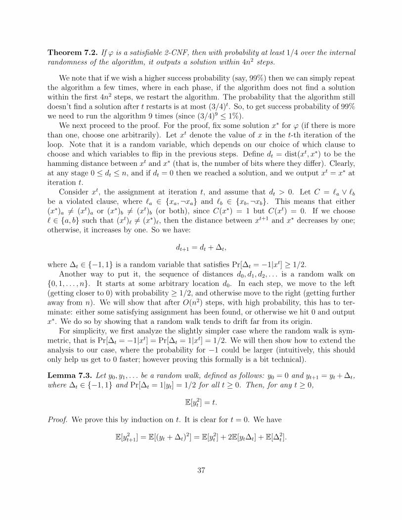
Lemma 7.3. Let y0, y1, . . . be a random walk, defined as follows: y0 = 0 and yt+1 = yt + ∆t,where ∆t ∈ −1, 1 and Pr[∆t = 1|yt] = 1/2 for all t ≥ 0. Then, for any t ≥ 0,
E[y2t ] = t.
Proof. We prove this by induction on t. It is clear for t = 0. We have
E[y2t+1] = E[(yt + ∆t)
2] = E[y2t ] + 2E[yt∆t] + E[∆2
t ].
37

By induction, E[y2t ] = t. Since ∆t ∈ −1, 1 we have E[∆2
t ] = 1. To conclude, we need toshow that E[yt∆t] = 0. We show this via the rule of conditional expectations:
E[yt∆t] = Eyt [E∆t [yt∆t|yt]] = Eyt [yt · E∆t [∆t|yt]] = Eyt [yt · 0] = 0.
We now prove the more general lemma, where we allow a consistent drift.
Lemma 7.4. Let y0, y1, . . . be a random walk, defined as follows: y0 = 0 and yt+1 = yt + ∆t,where ∆t ∈ −1, 1 and Pr[∆t = 1|yt] ≥ 1/2 for all t ≥ 0. Then, for any t ≥ 0,
E[y2t ] ≥ t/2.
Note that the same result holds by symmetry if we assume instead that Pr[∆t = −1|yt] ≥1/2 for all t ≥ 0.
Proof. The proof is by a “coupling argument”. Define a new random walk y′0, y′1, . . ., where
y′0 = 0, y′t+1 = y′t + ∆′t. In general, we would have that y′t,∆′t depend on y1, . . . , yt. So, fix
y1, . . . , yt, and assume that Pr[∆t = 1|yt] = α for some α ≥ 1/2. Define ∆′t as:
∆′t(yt,∆t) =
−1 if ∆t = −11 if ∆t = 1, with probability 1/2α−1 if ∆t = 1, with probability 1− 1/2α
It satisfies the following properties:
• ∆′t ≤ ∆t.
• Pr[∆′t = 1|y′t] = 1/2.
Note that the random walk y′0, y′1, . . . , is a symmetric random walk, which further satisfies
y′t ≤ yt for all t ≥ 0. By the previous lemma,
E[(y′t)2] = t.
Note moreover that since the random walk y′0, y′1, . . . is symmetric, Pr[y′t = a] = Pr[y′t = −a]
for any a ∈ Z. In particular, Pr[y′t ≥ 0] ≥ 1/2. Whenever y′t ≥ 0 we have y2t ≥ (y′t)
2. So wehave
E[y2t ] ≥ E[y2
t · 1y′t≥0] ≥ E[(y′t)2 · 1y′t≥0] = E[(y′t)
2]/2 = t/2.
We return now to the proof of Theorem 7.2. The proof will use Lemma 7.4, but theanalysis is more subtle.
38

Proof of Theorem 7.2. Recall that x0, x1, . . . is the sequence of “guesses” for a solution whichthe algorithm explores. Let T ∈ N denote the random variable of the step at which thealgorithm outputs a solution. The challenge in the analysis is that not only the sequence israndom, for also T is a random variable. For simplicity of notation later on, set xt = xT forall t > T .
Let y0, y1, . . . be defined as yt = dt − d0, where recall that dt = dist(xt, x∗). In order toanalyze this random walk, we define a new random walk z0, z1, . . . as follows: set zt = yt fort ≤ T , and for t ≥ T set zt+1 = zt + ρt, where ρt ∈ −1,+1 is uniformly and independentlychosen. We will argue that the sequence zt satisfies the conditions of Lemma 7.4. Namely,if we define ∆t = zt+1 − zt then Pr[∆t = −1|zt] ≥ 1/2.
To show this, let us condition on x0, . . . , xt. If none of them are solutions to ϕ then∆t = yt+1 − yt, and conditioned on x0, . . . , xt not being solutions, we already showed thatthe probability that ∆t = −1 is ≥ 1/2. If, on the other hand, x0, . . . , xt contain a solution,then ∆t = ρt and the probability that ∆t = −1 is exactly 1/2. In either case we have
Pr[∆t = −1|x0, . . . , xt] ≥ 1/2.
This then implies thatPr[∆t = −1|zt] ≥ 1/2.
Thus, we may apply Lemma 7.4 to the sequence z0, z1, . . . and obtain that for any t ≥ 1we have
E[z2t ] ≥ t/2.
Next, for t ≥ 1 let Tt = min(T, t). We may write zt as
zt = yTt +t−1∑i=Tt
ηi,
where the sum is empty if Tt = t. In particular, conditioning on T gives that
E[z2t |T ] = E
(yTt +t−1∑i=Tt
ηi
)2 ∣∣∣∣ T = E[y2
Tt |T ] + t− Tt.
Averaging over T gives then that
E[z2t ] = E[y2
Tt ] + t− E[Tt].
Next, observe that any yi = di − d0 is a difference of two numbers between 0 and n, andhence |yi| ≤ n. In particular, E[y2
Tt] ≤ n2. Thus we have
E[Tt] = E[y2Tt ] + t− E[z2
t ] ≤ n2 + t/2.
Wet t0 = 4n2. We haveE[Tt0 ] ≤ (3/4)t0.
39
By Markov inequality we have that
Pr[T ≥ t0] = Pr[Tt0 = t0] ≤ Pr[Tt0 ≥ (4/3)E[Tt0 ]] ≤ 3/4.
So, with probability at least 1/4, we have that T < t0, which means the algorithm finds asolution within t0 = 4n2 steps.
7.2 3-SAT
Let ϕ be a 3-CNF. Finding if ϕ has a satisfying assignment is NP-hard, and the best knownalgorithms take exponential time. However, we can still improve upon the naive 2n fullenumeration, as the following algorithm shows. The algorithm we analyze is due to Schoen-ing [Sch99].
Let m ≥ 1 be a parameter to be determined later.
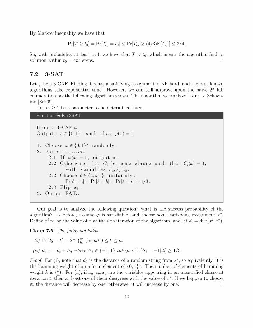
Function Solve-3SAT
Input : 3−CNF ϕOutput : x ∈ 0, 1n such that ϕ(x) = 1
1 . Choose x ∈ 0, 1n randomly .2 . For i = 1, . . . ,m :
2 . 1 I f ϕ(x) = 1 , output x .2 . 2 Otherwise , l e t Ci be some c l a u s e such that Ci(x) = 0 ,
with v a r i a b l e s xa, xb, xc .2 . 2 Choose ` ∈ a, b, c uni formly :
Pr[` = a] = Pr[` = b] = Pr[` = c] = 1/3 .2 . 3 F l ip x` .
3 . Output FAIL .
Our goal is to analyze the following question: what is the success probability of thealgorithm? as before, assume ϕ is satisfiable, and choose some satisfying assignment x∗.Define xi to be the value of x at the i-th iteration of the algorithm, and let di = dist(xi, x∗).
Claim 7.5. The following holds
(i) Pr[d0 = k] = 2−n(nk
)for all 0 ≤ k ≤ n.
(ii) dt+1 = dt + ∆t where ∆t ∈ −1, 1 satisfies Pr[∆t = −1|dt] ≥ 1/3.
Proof. For (i), note that d0 is the distance of a random string from x∗, so equivalently, it isthe hamming weight of a uniform element of 0, 1n. The number of elements of hammingweight k is
(nk
). For (ii), if xa, xb, xc are the variables appearing in an unsatisfied clause at
iteration t, then at least one of them disagrees with the value of x∗. If we happen to chooseit, the distance will decrease by one, otherwise, it will increase by one.
40
For simplicity, lets assume from now on that Pr[∆t = −1|dt] = 1/3, where the moregeneral case can be handled similar to the way we handled it for 2-SAT.
Claim 7.6. Assume that d0 = k. The probability that the algorithm finds a satisfying solutionis at least (
m
(m+ k)/2
)(1
3
)(m+k)/2(2
3
)(m−k)/2
.
Proof. Consider the sequence of steps ∆0, . . . ,∆m−1. If there are k more −1 than +1 in thissequence, then starting at d0 = k, we will reach dm = 0. The number of such sign sequencesis(
m(m+k)/2
), the probability for seeing a −1 is a 1/3, and the probability for seeing a +1 is
2/3.
Claim 7.7. For any 0 ≤ k ≤ n, the probability that the algorithms finds a solution is at least
2−n(n
k
)(m
(m+ k)/2
)(1
3
)(m+k)/2(2
3
)(m−k)/2
.
Proof. We require that d0 = k (which occurs with probability 2−n(nk
)) and, conditioned on
that occurring, apply Claim 7.6.
We now need to optimize parameters. Fix k = αn,m = βn for some constants α, β > 0.We will use the following approximation: for n ≥ 1 and 0 < α < 1,(
n
αn
)≈(
1
α
)αn(1
1− α
)(1−α)n
≈ 2H(α)n,
where H(α) = α log2( 1α
) + (1− α) log2( 11−α) is the entropy function. Then(
n
k
)≈ 2H(α)n,(m
(m+ k)/2
)≈ 2
H(
12
+α2β
)βn
(1
3
)(m+k)/2(2
3
)(m−k)/2
= 3−βn2(β−α)/2·n.
So, we can express the probability of success as ≈ 2−γn, where
γ = 1−H(α)−H(
12
+ α2β
)β + log2 3 · β − β−α
2.
Our goal is to choose 0 < α < 1 and β ≥ α to minimize γ. The minimum is obtained forα = 1/3, β = 1, which gives γ ≈ 0.41.
So, we have an algorithm that runs in time O(m) = O(n), and finds a satisfiable assign-ment with probability ≈ 2−γn. To find a satisfiable assignment with high probability, wesimply repeat it N = 5 · 2γn times. The probability it fails in all these executions is at most
(1− 2−γn)N ≤ exp(−2−γnN) ≤ exp(−5) ≤ 1%.
Corollary 7.8. We can solve 3-SAT in time O(2γn) for γ ≈ 0.41.
41
8 Hash functions: the power of pairwise independence
Hash functions are used to map elements from a large domain to a small one. They are com-monly used in data structures, cryptography, streaming algorithms, coding theory, and more- anywhere where we want to store efficiently a small subset of a large universe. Typically,for many of the applications, we would not have a single hash function, but instead a familyof hash functions, where we would randomly choose one of the functions in this family asour hash function.
Let H = h : U → R be a family of functions, mapping elements from a (typicallylarge) universe U to a (typically small) range R. For many applications, we would like two,seemingly contradicting, properties from the family of functions:
• Functions h ∈ H should “look random”
• Functions h ∈ H are succinctly described, and hence processed and stored efficiently.
The way to resolve this is to be more specific about what do we mean by “lookingrandom”. The following definition is such a concrete realization, which although is quiteweak, it is already very useful.
Definition 8.1 (Pairwise independent hash functions). A family H = h : U → R issaid to be pairwise independent, if for any two distinct elements x1 6= x2 ∈ U , and any two(possibly equal) values y1, y2 ∈ R,
Prh∈H
[h(x1) = y1 and h(x2) = y2] =1
|R|2.
We investigate the power of pairwise independent hash functions in this chapter, anddescribe a few applications. For many more applications we recommend the book [LLW06].
8.1 Pairwise independent bits
To simplify notations, let us consider the case of R = 0, 1. We also assume that |U | = 2k
for some k ≥ 1, by possibly increasing the size of the universe by a factor of at most two.Thus, we can identify U = 0, 1k, and identify functions h ∈ H with boolean functionsh : 0, 1k → 0, 1. Consider the following construction:
H2 = ha,b(x) = 〈a, x〉+ b (mod 2) : a ∈ 0, 1k, b ∈ 0, 1.
One can check that |H2| = 2k+1 = 2|U |, which is much smaller than the set of all functionsfrom 0, 1k to 0, 1 (which has size 22k). We will show that H2 is pairwise independent.To do so, we need the following claim.
Claim 8.2. Fix a x ∈ 0, 1k, x 6= 0k. Then
Pra∈0,1k
[〈a, x〉 (mod 2) = 0] =1
2.
42

Proof. Fix i ∈ [k] such that xi = 1. Then
Pra∈0,1k
[〈a, x〉 (mod 2) = 0] = Pr
[ai =
∑j 6=i
ajxj (mod 2)
]=
1
2.
Lemma 8.3. H2 is pairwise independent.
Proof. Fix distinct x1, x2 ∈ 0, 1k and (not necessarily distinct) y1, y2 ∈ 0, 1. In all thecalculations below of 〈a, x〉+ b, we evaluate the result modulo 2. We need to prove
Pra∈0,1k,b∈0,1
[〈a, x1〉+ b = y1 and 〈a, x2〉+ b = y2] =1
4.
If we just randomized over a then by Claim 8.2, for any y ∈ 0, 1 we have
Pra
[〈a, x1〉 ⊕ 〈a, x2〉 = y] = Pra
[〈a, x1 ⊕ x2〉 = y] =1
2.
Randomizing also over b gives us the desired result:
Pra,b
[〈a, x1〉+ b = y1 and 〈a, x2〉+ b = y2] =
Pra,b
[〈a, x1〉 ⊕ 〈a, x2〉 = y1 ⊕ y2 and b = 〈a, x1〉+ y1] =
1
2· 1
2=
1
4.
Next, we describe an alternative viewpoint, which will justify the name ”pairwise inde-pendent bits”.
Definition 8.4 (Pairwise independent bits). A distribution D over 0, 1n is said to bepairwise independent, if for any distinct i, j ∈ [n] and any y1, y2 ∈ 0, 1 we have
Prx∼D
[xi = y1 and xj = y2] =1
4.
We note that we can directly use H2 to generate pairwise independent bits. Assumethat n = 2k. Identify h ∈ H2, h : 0, 1k → 0, 1, with the string uh in0, 1n giving byconcatenating all the evaluations of h is some pre-fixed order. Let D be the distribution over0, 1n obtained by sampling h ∈ H2 uniformly and outputting uh. Then the condition thatD is pairwise independent is equivalent to that of H2 be pairwise independent. Note thatthe construction above gives a distribution D supported on |H2| = 2n elements in 0, 1n,much less than the full space. In particular, we can represent a string u in the support of Dby specifying the hash function which generated it, which only requires log |H| = log n + 1bits.
Example 8.5. Let n = 4. A uniform string from the following set of 8 = 23 strings ispairwise independent:
0000, 0011, 0101, 0110, 1001, 1010, 1100, 1111.
43

8.2 Application: de-randomized MAXCUT
Let G = (V,E) be a simple undirected graph. For S ⊂ V let E(S, Sc) = (u, v) ∈ E : u ∈S, v ∈ Sc be the number of edges which cross the cut S. The MAXCUT problem asks tofind the maximal number of edges in a cut.
MAXCUT(G) = maxS⊂V|E(S, Sc)|.
Computing the MAXCUT of a graph is known to be NP-hard. Still, there is a simplerandomized algorithm which approximates it within factor 2. Below, let V = v1, . . . , vn.Lemma 8.6. Let x1, . . . , xn ∈ 0, 1 be uniformly and independently chosen. Set
S = vi : xi = 1.
Then
ES[|E(S, Sc)|] ≥ |E(G)|2
≥ MAXCUT(G)
2.
Proof. For any choice of S we have
|E(S, Sc)| =∑
(vi,vj)∈E
1vi∈S1vj∈Sc .
Note that every undirected edge u, v in G is actually counted twice in the calculationabove, once as (u, v) and once as (v, u). However, clearly at most one of these is in E(S, Sc).By linearity of expectation, the expected size of the cut is
ES[|E(S, Sc)|] =∑
(vi,vj)∈E
E[1vi∈S1vj /∈S] =∑
(vi,vj)∈E
E[1xi=11xj=0]
=∑
(vi,vj)∈E
Pr[xi = 1 and xj = 0] = 2|E(G)| · 1
4=|E(G)|
2.
This implies that a random choice of S has a non-negligible probability of giving a 2-approximation.
Corollary 8.7. PrS
[|E(S, Sc)| ≥ |E(G)|
2
]≥ 1
2E(G)≥ 1
n2 .
Proof. Let X = |E(S, Sc)| be a random variable counting the number of edges in a randomcut. Let µ = |E(G)|/2, where we know that E[X] ≥ µ. Note that whenever X < µ, wein fact have that X ≤ µ − 1/2, since X is an integer and µ a half-integer. Also, note thatalways X ≤ |E(G)| ≤ 2µ. Let p = Pr[X ≥ µ]. Then
E[X] = E[X|X ≥ µ] Pr[X ≥ µ] + E[X|X ≤ µ− 1/2] Pr[X ≤ µ− 1/2]
≤ 2µ · p+ (µ− 1/2) · (1− p)≤ µ− 1/2 + 2µp.
So we must have 2µp ≥ 1/2, which means that p ≥ 1/(4µ) ≥ 1/(2E(G)).
44

In particular, we can sample O(n2) sets S, compute for each one its cut size, and we areguaranteed that with high probability, the maximum will be at least |E(G)|/2.
Next, we derandomize this randomized algorithm using pairwise independent bits. Asa side benefit, it will reduce the computation time from testing O(n2) sets to testing onlyO(n) sets.
Lemma 8.8. Let x1, . . . , xn ∈ 0, 1 be pairwise independent bits (such as the ones given byH2). Set
S = vi : xi = 1.Then
ES[|E(S, Sc)|] ≥ |E(G)|2
.
Proof. The only place where we used the fact that the bits were uniform in the proof ofLemma 8.6, was in the calculation
Pr[xi = 1 and xj = 0] =1
4
for all distinct i, j. However, this is also true for pairwise independent bits (by definition).
In particular, for one of the O(n) sets S that we generate in the algorithm, we must havethat |E(S, Sc)| exceeds the average, and hence |E(S, Sc)| ≥ |E(G)|/2.
8.3 Optimal sample size for pairwise independent bits
The previous application showed the usefulness of having small sample spaces for pairwiseindependent bits. We saw that we can generate O(n) binary strings of length n, such thatchoosing one of them uniformly gives us pairwise independent bits. We next show that thisis optimal.
Lemma 8.9. Let X ⊂ 0, 1n and let D be a distribution supported on X. Assume that Dis pairwise independent. Then |X| ≥ n.
Proof. Let X = x1, . . . , xm and let pi = Pr[D = xi]. For any i ∈ [n], we construct a vectorvi ∈ Rm as follows:
(vi)` =√p` · (−1)(x`)i .
We will show that the set of vectors v1, . . . , vn are linearly independent in Rm, and hencewe must have |X| = m ≥ n.
As a first step, we show that 〈vi, vj〉 = 0 for all i 6= j:
〈vi, vj〉 =m∑`=1
p` · (−1)(x`)i+(x`)j = Ex∼D[(−1)xi+xj
]= Pr
x∼D[xi + xj = 0 (mod 2)]− Pr
x∼D[xi + xj = 1 (mod 2)]
=1
2− 1
2= 0.
45

Next, we show that this implies that v1, . . . , vn must be linearly independent. Assumetowards contradiction that this is not the case. That is, there exist coefficients α1, . . . , αn ∈R, not all zero, such that ∑
αivi = 0.
However, for any j ∈ [n], we have
0 =⟨∑
αivi, vj
⟩=∑
αi 〈vi, vj〉 = αj‖vj‖2 = αj.
So αj = 0 for all j, a contradiction. Hence, v1, . . . , vn are linearly independent and hence|X| = m ≥ n.
8.4 Hash functions with large ranges
We now consider the problem of constructing a family of hash functions H = h : U → Rfor large R. For simplicity, we will assume that |R| is prime, although this requirement canbe somewhat removed. So, lets identify R = Fp for a prime p. We may assume that |U | = pk,by possibly increase the size of the universe by a factor p. This allows us to identify U = Fkp.Define the following family of hash functions:
Hp = ha,b(x) = 〈a, x〉+ b : a ∈ Fkp, b ∈ Fp.
Note that |H| = pk+1 = |U | · |R|, and observe that for p = 2 this coincides with our previousdefinition of H2. We will show that Hp is pairwise independent. As before, we need anauxiliary claim first.
Claim 8.10. Let x ∈ Fkp, x 6= 0. Then for any y ∈ Fp,
Pra∈Fk
p
[〈a, x〉 = y] =1
p.
Proof. Fix i ∈ [k] such that xi 6= 0. Then
Pra∈Fk
p
[〈a, x〉 = y] = Pr
[aixi = y −
∑j 6=i
ajxj
].
Now, for every fixing of aj : j 6= i, we have that aixi is uniformly distributed in Fp, hencethe probability that it equals any specific value is exactly 1/p.
Lemma 8.11. Hp is pairwise independent.
Proof. Fix distinct x1, x2 ∈ Fkp and (not necessarily distinct) y1, y2 ∈ Fp. All the calculationsbelow of 〈a, x〉+ b are in Fp. We need to show
Pra∈Fk
p ,b∈Fp
[〈a, x1〉+ b = y1 and 〈a, x2〉+ b = y2] =1
p2.
46

If we just randomized over a then by the claim, then for any y ∈ Fp by the claim,
Pra
[〈a, x1〉 − 〈a, x2〉 = y] = Pra
[〈a, x1 − x2〉 = y] =1
p.
Randomizing also over b gives us the desired result.
Pra,b
[〈a, x1〉+ b = y1 and 〈a, x2〉+ b = y2] =
Pra,b
[〈a, x1〉 − 〈a, x2〉 = y1 − y2 and b = 〈a, x1〉+ y1] =
1
p· 1
p=
1
p2.
8.5 Application: collision free hashing
Let S ⊂ U be a set of objects. A hash function h : U → R is said to be collision free for S ifit is injective on S. That is, h(x) 6= h(y) for all distinct x, y ∈ S. We will show that if R islarge enough, then any pairwise independent hash family contains many collision free hashfunctions for any small set S. This is extremely useful: it allows to give lossless compressionof elements from a large universe to a small range.
Lemma 8.12. Let H : h : U → R be a pairwise independent hash family. Let S ⊂ U be aset of size |S|2 ≤ |R|. Then
Prh∈H
[h is collision free for S] ≥ 1/2.
Proof. Let h ∈ H be uniformly chosen, and let X be a random variable that counts thenumber of collisions in S. That is,
X =∑x,y⊂S
1h(x)=h(y).
The expected value of X is
E[X] =∑x,y⊂S
Prh∈H
[h(x) = h(y)] =
(|S|2
)1
|R|≤ |S|
2
2|R|≤ 1
2.
By Markov’s inequality,
Prh∈H
[h is not collision free for S] = Pr[X ≥ 1] ≤ 1/2.
47
8.6 Efficient dictionaries: storing sets efficiently
We now show how to use pairwise independent hash functions, in order to design efficientdictionaries. Fix a universe U . For simplicity, we will assume that for any R we have afamily of pairwise independent hash functions H = h : U → R, and note that while ourprevious constructions required R to be prime (or in fact, a prime power), this will at mostdouble the size of the range, which at the end will only change our space requirements by aconstant factor.
Given a set S ⊂ U of size |S| = n, we would like to design a data structure which supportsqueries of the form “is x ∈ S”? Our goal will be to do so, while minimizing both the spacerequirements and the time it takes to answer a query. If we simply store the set as a sortedlist of n elements, then the space (memory) requirements are O(n log |U |), and each querytakes time O(log |U | + log n), by doing a binary search on the list. We will see that thesecan be improved via hashing.
First, consider the following simple hashing scheme. Fix a range R = 1, . . . , n2. LetH = h : U → [n2] be a pairwise independent hash function. We showed that a randomlychosen h ∈ H will be collision free on S with probability at least 1/2. So, we can sampleh ∈ H until we find such an h, which on average would require two attempts. Let A be anarray of length n2. It will be mostly empty, except that we set A[h(x)] = x for all x ∈ S.Now, to check whether x ∈ S, we compute h(x) and check whether A[h(x)] = x or not.Thus, the query time is only O(log |U |). However, we pay in our space requirements are big:to store n elements, we maintain an array of size n2, which requires at least n2 bits (andpossibly even O(n2 log |U |), depending on how efficient we are in storing the empty cells).
We describe a two-step hashing scheme due to Fredman, Komlos and Szemeredi [FKS84]which avoids this large waste of space. It will use only O(n log n+ log |U |) space, but wouldstill allow for query time of O(log |U |). As a preliminary step, we apply the collision freehash scheme we just described. So, may assume from now on that U = O(n2) and thatS ⊂ U has size |S| = n.
Step 1. We first find a hash function h : U → [n] which has only n collisions. Let Coll(h, S)denote the number of collisions of h for S, namely
Coll(h, S) = |x, y ⊂ S : h(x) = h(y)|].
If H = h : U → [n] is a family of pairwise independent hash functions, then
Eh∈H[Coll(h, S)] =∑x,y⊂S
Pr[h(x) = h(y)] =
(|S|2
)1
n≤ |S|
2
2n≤ n
2.
By Markov’s inequality, we have
Prh∈H
[Coll(h, S) ≥ n] ≤ 1/2.
So, after on average two iterations of randomly choosing h ∈ H, we find such a functionh : U → [n] such that Coll(h, S) ≤ n. We fix it from now on. Note that it is representedusing only O(log n) bits.
48

Step 2. Next, for any i ∈ [n] let Si = x ∈ S : h(x) = i. Observe that∑|Si| = n and
n∑i=1
(|Si|2
)= Coll(h, S) ≤ n.
Let ni = |Si|2. Note that∑ni = 2Coll(h, S) +
∑|Si| ≤ 3n. We will find hash functions
hi : U → [ni] which are collision free on Si. Choosing a uniform hash function from apairwise independent set of hash functions Hi = h : U → [ni] succeeds on average aftertwo samples. So, we only need O(n) time in total (on expectation) to find these functions.As each hi requires O(log n) bits to be represented, we need in total O(n log n) to representall of them.
Let A be an array of size 3n. Let offseti =∑
j<i nj. The sub-array A[offseti : offseti +ni]will be used to store the elements of Si. Initially A is empty. We set
A[offseti + hi(x)] = x ∀x ∈ Si.
Note that there are no collisions in A, as we are guaranteed that hi are collision free on Si.We will also keep the list of offseti : i ∈ [n] in a separate array.
Query. To check whether x ∈ S, we do the following:
• Compute i = h(x).
• Read offseti.
• Check if A[offseti + hi(x)] = x or not.
This can be computed using O(log n) bit operations.
Space requirements. The hash functions h requires O(log n) bits. The hash functionshi : i ∈ [n] require O(n log n) bits. The array A requires O(n log n) bits.
Setup time. The setup algorithm is randomized, as it needs to find good hash functions.It has expected running time is O(n log n) bit operations.
• To find h takes O(n log n) time, as this is how long it takes to verify that it is collisionfree.
• To find each hi takes O(|Si| log n) time, and in total it is O(n log n) time.
• To set up the arrays of offseti : i ∈ [n] and A takes O(n log n) time.
RAM model vs bit model. Up until now, we counted bit operations. However, com-puters can operate on words efficiently. A model for that is the RAM model, where we canperform basic operations on log n-bit words. In this model, it can be verified that the querytime is O(1) word operations, space requirements are O(n) words and setup time is O(n)word operations.
49

8.7 Bloom filters
Bloom filters allow for even more efficient data structures for set membership, if some errorsare allowed. Let U ba a universe, S ⊂ U a subset of size |S| = n. Let h : U → [m] be auniform hash function, for m to be determined later. The data structure maintains a bitarray A of length m, initially set to zero. Then, for every x ∈ S, we set A[h(x)] = 1. In orderto check if x ∈ S, we compute h(x), read the value A[h(x)] we answer “yes” if A[h(x)] = 1and “no” otherwise. This has the following guarantees:
• No false negative: if x ∈ S we will always say “yes”.
• Few false positives: if x /∈ S, we will say “yes” with probability |i:A[i]=1|m
, assuming his a fully random function.
So, if for example we set m = 2n, then the probability for x /∈ S that we say ”no” it at least1/2. In fact, the probability is greater, since when hashing n elements to 2n values therewill be some collisions, and so the number of 1’s in the array will be less than n. It turnsout that to get probability 1/2 we only need m ≈ 1.44n. This is since, the probability thatA[i] = 1, over the choice of h, is
Prh
[A[i] = 0] = Pr[h(x) 6= i, ∀x ∈ S] =
(1− 1
m
)n≈ e−n/m.
So, for m = n/ln(2) ≈ 1.44n, the expected number of 0’s in A is m/2.Note that a bloom filter uses O(n) bits, which is much less than the O(n log |U |) bits we
needed when we did not allow for any errors. It can be shown that we don’t need h to beuniform (which can be costly to store); a k-wise independent hash family (an extension ofpairwise independent) for k = O(log n) suffices, and such a function can be stored using onlyO(log2 n) bits.
50
9 Min cut
Let G = (V,E) be a graph. A cut in this graph is |E(S, Sc)| for some S ⊂ V , that is,the number of edges which cross a partition of the vertices. Finding the maximum cut isNP-hard, and the best algorithms solving it run in exponential time. We saw an algorithmwhich finds a 2-approximation for the max-cut. However, finding the minimum cut turnsout to be solvable in polynomial time. Today, we will see a randomized algorithm due toKarger [Kar93] which achieves this is a beautiful way. To formalize this, the algorithm willfind
min-cut(G) = min∅6=S(V
|E(S, Sc)|.
9.1 Karger’s algorithm
The algorithm is very simple: choose a random edge and contract it. Repeat n − 1 times,until only two vertices remain. Output this as a guess the for min-cut. We will show thatthis outputs the min-cut with probability at least 2/n2, hence repeating it 3n2 times (say)will yield a min-cut with probability at least (1− 2/n2)3n2 ≥ 99%.
Formally, to define a contraction we need to allow graphs to have parallel edges.
Definition 9.1 (edge contraction). Let G = (V,E) be an undirected graph with |V | = nvertices, potentially with parallel edges. For an edge e = (u, v) ∈ E, the contraction of Galong e is an undirected graph on n − 1 vertices, where we merge u, v to be a single node,and delete any self-loops that may be created in this process.
We can now present the algorithm.
Karger
Input : Undirected graph G = (V,E) with |V | = nOutput : Cut in G
1 . Let Gn = G .2 . For i = n, . . . , 3 do :2 . 1 Choose a uniform edge ei ∈ Gi .2 . 2 Set Gi−1 to be the con t ra c t i on o f Gi along ei .3 . Output the cut in G cor re spond ing to G2 .
Next, we proceed to analyze the algorithm. We start with a few observations. Bycontracting along an edge e = (u, v), we make a commitment that u, v belong to the sameside of the cut, so we restrict the number of potential cuts. Hence, any cut of Gi is a cut ofG, and in particular
min-cut(G) ≤ min-cut(Gi), i = n, . . . , 2.
51

In order to analyze the algorithm, lets fix from now on a min-cut S ⊂ V (G). We willanalyze the probability that the algorithm never chooses an edge in S. Hence, after n − 2contractions, the output will be exactly the cut S. First, we bound the min-cut by cuts forwhich one side is a single vertex.
Claim 9.2. min-cut(G) ≤ minv∈G deg(v) ≤ 2 |E||V | .
Proof. For any vertex v ∈ V , we can form a cut by taking E(v, V \ v). It has deg(v)many edges. Since 2|E| =
∑v∈V deg(v) we can bound
min-cut(G) ≤ minv∈V
deg(v) ≤ 2|E||V |
.
Claim 9.3. Let G = (V,E) be a graph, S ⊂ V be a minimal cut in G. Let e ∈ E be auniform chosen edge. Then
Pre∈E
[e ∈ E(S, Sc)] ≤ 2
|V |.
Proof. We saw that |E(S, Sc)| ≤ 2|E|/|V |. So, the probability that e is in the cut is
Pre∈E
[e ∈ E(S, Sc)] ≤ |E(S, Sc)||E|
≤ 2|E|/|V ||E|
≤ 2
|V |.
Theorem 9.4. For any min-cut S in G, Pr[algorithm outputs S] ≥ 1
(n2)≥ 2
n2 .
Proof. Fix a min-cut S ⊂ V . The algorithm outputs S if it never chooses an edge in S. So
Pr[algorithm outputs S] = Pr[en, . . . , e3 /∈ E(S, Sc)]
=3∏i=n
Pr[ei /∈ E(S, Sc)|en, . . . , ei+1 /∈ E(S, Sc)].
To analyze this, assume that en, . . . , ei+1 /∈ E(S, Sc), so that S is still a cut in Gi. Thus, it isalso a min-cut in Gi, and we proved that in this case, Pr[ei ∈ E(S, Sc)] ≤ 1/2|V (Gi)| = 1/2i.So
Pr[algorithm outputs S] ≥(
1− 2
n
)(1− 2
n− 1
). . .
(1− 2
3
)=n− 2
n· n− 3
n− 1· n− 4
n− 2· . . . · 2
4· 1
3
=2
n(n− 1).
We get a nice corollary: the number of min-cuts in G is at most(n2
). Can you prove it
directly?
52

9.2 Improving the running time
The time it takes to find a min-cut by Karger’s algorithm described above is O(n4): we needO(n2) iterations to guarantee success with high probability. Every iteration requires n − 2rounds of contraction, and every contraction takes O(n) time. We will see how to improvethis running time to O(n2 log n) due to Karger and Stein [KS96]. The main observationguiding this is that most of the error comes when the graph becomes rather small; however,when the graphs are small, the running time is also smaller. So, we can allow to run multipleinstances for smaller graphs, which would boost the success probability without increasingthe running time too much.
Fast-Karger
Input : Undirected graph G = (V,E) with |V | = nOutput : Cut in G
0 . I f n = 2 output the only p o s s i b l e cut .
1 . Let Gn = G and m = n/√
2 .2 . For i = n, . . . ,m+ 1 do :2 . 1 Choose a uniform edge ei ∈ Gi .2 . 2 Set Gi−1 to be the con t ra c t i on o f Gi along ei .3 . Run r e c u r s i v e l y Si = Fast-Karger(Gi) f o r i = 1, 2 .4 . Output S ∈ S1, S2 which minimizes E(S, Sc) .
Claim 9.5. Fix a cut S. Run the original Karger algorithm, but output Gm for m = n/√
2.Then the probability that S is still a cut in Gm is at least 1/2.
Proof. Repeating the analysis we did, but stopping once we reach Gm, gives
Pr[S is a cut of Gm] = Pr[en, . . . , em+1 /∈ E(S, Sc)] ≥ n− 2
n· . . . · m− 1
m+ 1=m(m− 1)
n(n− 1).
So, if we set m = n/√
2, this probability is at least 1/2.
Theorem 9.6. Fast-Karger runs in time O(n2 log n) and returns a minimal cut with prob-ability at least 1/4.
Proof. We first analyze the success probability. Let P (n) be the probability that the algo-rithm succeeds on graphs of size n. We will prove by induction that P (n) ≥ 1/4. We provedthat
Pr[min-cut(Gm) = min-cut(G)] ≥ 1
2.
So we have
P (n) ≥ 1
2· (1− P (m))2 ≥ 1
2·(
3
4
)2
=9
32≥ 1
4.
53

We next analyze the running time. Let T (n) be the running time of the algorithm on graphsof size n. Then
T (n) = 2 · T (n/√
2) +O(n2).
This solves to T (n) = O(n2 log n).
54

10 Routing
Let G = (V,E) be an undirected graph, where nodes represent processors and edges representcommunication channels. Each node wants to send a message to another node: v → π(v),where π is some permutation on the vertices. However, messages can only traverse on edges,and each edge can only carry one message at a given time unit. A routing scheme is a methodof deciding on pathes for the messages obeying these restrictions, which tries to minimizethe time it takes for all messages to reach their destination. If more than one packet needsto traverse an edge, then only one packet does so at any unit time, and the rest are queuedfor later time steps. The order of sending the remaining packets does not matter much. Forexample, you can assume a FIFO (First In First Out) queue on every edge.
Here, we will focus on the hypercube graph H, which is a common graph used in dis-tributed computation.
Definition 10.1 (Hypercube graph). The hypercube graph Hn = (V,E) has vertices corre-sponding to all n-bit strings V = 0, 1n and edges which correspond to bit flips,
E = (x, x⊕ ei) : x ∈ 0, 1n, i ∈ [n],
where ei is the i-th unit vector, and ⊕ is bitwise xor.
An oblivious routing scheme is a scheme where the path of sending v → π(v) dependsjust on the endpoints v, π(v), and not on the targets of all other messages. Such schemesare easy to implement, as each node v can compute them given only their local knowledgeof their target π(v). A very simple one for the hypercube graph is the “bit-fixing scheme”:in order to route v = (v1, . . . , vn) to u = (u1, . . . , un), we flip the bits in order whenevernecessary. So for example, the path from v = 10110 to u = 00101 is
10110→ 00110→ 00100→ 00101.
We denote by Pfix(v, u) the path from v to u according to the bit-fixing routing scheme.
10.1 Deterministic routing is bad
Although the maximal distance between pairs of vertices in H is n, routing based on thebit-fixing scheme can incur a very large overhead, due to the fact that edges can only carryone message at a time.
Lemma 10.2. There exists a permutation π : 0, 1n → 0, 1n for which the bit-fixingscheme requires at least 2n/2/n time steps to transfer all messages.
Proof. Assume n is even, and write x ∈ 0, 1n as x = (x′, x′′) with x′, x′′ ∈ 0, 1n. Considerany permutation π : 0, 1n → 0, 1n which maps (x′, 0) to (0, x′) for all x′ ∈ 0, 1n/2.These 2n/2 pathes all pass through a single vertex (0, 0). As it has only n outgoing edges,we need at least 2n/2/n time steps to send all these packages.
55
In fact, a more general theorem is true, which shows that any deterministic obliviousrouting scheme is equally bad. A deterministic routing scheme for a graph G = (V,E) is arouting scheme, that specifies in advance for any two nodes u, v ∈ V a path P (u, v) in G. Ifa permutation π maps u to v, then the message from u to v has the follow this one path.
Kaklamanis et al. [KKT91] proved that in any N node graph of degree d, any determin-istic routing scheme requires in the worst case Ω(
√N/d) time steps. When applied to the
hypercube, it shows that any deterministic routing scheme requires at least Ω(2n/2/n) timesteps in the worst case, matching our bound for the bit-fixing scheme.
Theorem 10.3. Let G = (V,E) be a graph on N nodes with maximal degree d. Fix anydeterministic routing scheme for G. Then there exists a permutation π : V → V for whichsome edge e ∈ E is contained in at least Ω(
√N/d) paths given by the routing scheme. In
particular, we need at least Ω(√N/d) time steps to send all the messages.
Proof. For every nodes u, v ∈ V let P (u, v) denote the path from u to v fixed by thedeterministic routing scheme. For every u, let Gu denote the graph given by the union ofall P (u, v) : v 6= u, where edges are taken with multiplicity. For a parameter k ≥ 1 to bedetermined later, let Su denote the set of edges in Gu which have multiplicity ≥ k; namely,they are contained in at least k paths P (u, v) for v 6= u. Let Vu denote the set of verticesadjacent to Su. We will assume that k ≤ (N − 1)/d, so that by definition u ∈ Vu (as thereare N − 1 choices for v 6= u and only ≤ d edges that are adjacent to u). Note furthermorethat |Vu| ≤ 2|Su|.
We first show that Vu is large for every u ∈ V . Concretely, we will show that
|V \ Vu| ≤ kd|Vu|.
To do that, we will assign a node in Vu for every node in V \ Vu, and argue that everynode in Vu is assigned at most (k − 1)(d − 1) times. So, fix v ∈ V \ Vu. Let P (u, v) beu = v0, v1, . . . , vt = v. We assign to v the last vertex in this path which is in Vu. There is atleast one such vertex, as u ∈ Vu. Assume this vertex is vi, where i < t. Then vi+1 /∈ Vu. Thismeans that the edge (vi, vi+1) is not in Su, which means that it is contained in ≤ k pathsstarting at u. The vertex vi can then be assigned to at most kd nodes in V \ Vu (there are≤ d edges leaving it; and only edges which are contained in < k paths can be used).
This then implies that
N = |V | ≤ (kd+ 1)|Vu| ≤ 2kd|Vu| ≤ 4kd|Su|.
This implies that
|Su| ≥N
4kd.
We next use an averaging argument. For an edge e let ne = |u : e ∈ Su| denote thenumber of times the edge e is contained in some Su. Then∑
e∈E
ne =∑u∈V
|Su| ≥N2
4kd.
56

Hence there exists e ∈ E for which
ne ≥N2
4kd|E|≥ N
2kd2.
Fix k so that k ≈ N2kd2
, which gives k ≈√N/2/d. The edge e is contained in say
Su1 , . . . , Suk for some distinct nodea u1, . . . , uk ∈ V . As |Sui | ≥ k, we can (greedily) choosenodes v1, . . . , vk ∈ V such that vi ∈ Sui and v1, . . . , vk are all distinct. Then all the pathesP (ui, vi) contain the edge e. To conclude, complete the partial permutation mapping eachui to vi to a complete permutation.
10.2 Randomized routing saves the day
We will consider the following oblivious routing scheme, which we call the two-step bit-fixingscheme. It uses randomness on top of the deterministic bit-fixing routing scheme describedearlier.
Definition 10.4 (Two-step bit fixing scheme). In order to route a packet from a sourcev ∈ 0, 1n to a target π(v) ∈ 0, 1n do the following:
(i) Sample uniformly an intermediate target t(v) ∈ 0, 1n.
(ii) Follow the path Pfix(v, t(v)).
(iii) Follow the path Pfix(t(v), π(v)).
Observe that t : 0, 1n → 0, 1n is not necessarily a permutation, as each t(v) issampled independently, and hence there could be collisions. Still, we prove that with veryhigh probability, all packets will be delivered in linear time.
Theorem 10.5. With probability ≥ 1−2−(n−1), all packets will be routed to their destinationsin at most 14n time steps.
In preparation for proving it, we first prove a few results about the deterministic bit-fixingrouting scheme.
Claim 10.6. Let v, v′, u, u′ ∈ 0, 1n. Let P = Pfix(v, u) and P ′ = Pfix(v′, u′). If the pathsseparate at some point, they never re-connect. That is, let w1, . . . , wm be the vertices of Pand let w′1, . . . , w
′m′ be the vertices of P ′. Assume that wi = w′j but wi+1 6= w′j+1. Then
w` 6= w′`′ ∀` ≥ i+ 1, `′ ≥ j + 1.
Proof. By assumption wi = w′j and wi+1 6= w′j+1. Then wi+1 = wi ⊕ ea and w′j+1 = w′j ⊕ ebwith a 6= b. Assume without loss of generality that a < b. Then (w`)a = (wi+1)a = (wi)a⊕ 1for all ` ≥ i + 1, while (w′`′)a = (w′j+1)a = (w′j)a = (wi)a for all `′ ≥ j + 1. Thus, for any` ≥ i+1, `′ ≥ j+1 we have w` 6= w′`′ , which means that the pathes never intersect again.
57
Lemma 10.7. Fix π : 0, 1n → 0, 1n and v ∈ 0, 1n. Let e1, . . . , ek be the edges ofPfix(v, π(v)). Define
Sv = v′ ∈ V : v′ 6= v, Pfix(v′, π(v′)) contains some edge from e1, . . . , ek.
Then the packet sent from v to π(v) will reach its destination after at most k + |Sv| steps.
Proof. Let S = Sv for simplicity of notation. The proof is by a charging argument. Let pv bethe packet sent from v to π(v). We assume that packets carry “tokens” on them. Initially,there are no tokens. Assume that at some time step, the packet pv it is supposed to traversean edge ei for some i ∈ [k], but instead another packet pv′ is sent over ei at this time step(necessarily v′ ∈ S). In such a case, we generate a new token and place it on pv′ . Next, iffor some v′ ∈ S, a packet pv′ with at least one token on it is supposed to traverse an edgeej for j ∈ [k], but instead another packet pv′′ is sent over it at the same time step (again,necessarily v′′ ∈ S), then we move one token from pv′ to pv′′
We will show that any packet pv′ for v′ ∈ S can have at most one token on it at any givenmoment. This shows that at most |S| tokens are generated overall. Thus, pv is delayed forat most |S| steps and hence reaches its destination after at most k + |S| steps.
To see that, observe that tokens always move forward along e1, . . . , ek. That is, if wefollow a specific token, it starts at some edge ei, follows a path ei, . . . , ej for some j ≥ i, andthen traverses an edge outside e1, . . . , ek. At this point, by Claim 10.6, it can never intersectthe path e1, . . . , ek again. So, we can never have two tokens which traverse the same edge atthe same time, and hence two tokens can never be on the same packet.
Lemma 10.8. Let t : 0, 1n → 0, 1n be uniformly chosen. Let P (v) = Pfix(v, t(v)). Thenwith probability at least 1− 2−n over the choice of t, for any path P (v), there are at most 6nother pathes P (w) which intersect some edge of P (v).
Proof. For v, w ∈ 0, 1n, let Xv,w ∈ 0, 1 be the indicator random variable for the eventthat P (v) and P (w) intersect in an edge. Our goal is to upper bound Xv =
∑w 6=vXv,w for
all v ∈ 0, 1n. Before analyzing it, we first analyze a simpler random variable.Fix an edge e = (u, u ⊕ ea). For v ∈ 0, 1n, let Ye,w ∈ 0, 1 be an indicator variable
for the event that the edge e belongs to the path P (w). The number of pathes which passthrough e is then
∑w∈0,1n Ye,w. Now, the path between w and t(w) passes through e iff
wi = ui for all i > a, and t(w)i = ui for all i < a. Let Ae = w ∈ 0, 1n : wi = ui ∀i > a.Only w with w ∈ Ae has a nonzero probability for the path from w to t(w) to go throughe. Note that |Ae| = 2a. Moreover, for any w ∈ Ae, the probability that P (w) indeed passesthrough e is given by
Pr[Ye,w = 1] = Pr[t(w)i = ui ∀i < a] = 2−(a−1).
Hence, the expected number of pathes P (w) which go through any edge e is at most 2, since
E
∑w∈0,1n
Ye,w
=∑w∈Ae
Pr[Ye,w = 1] = 2a · 2−(a−1) = 2.
58

Next, the pathes P (v), P (w) intersect if some e ∈ P (v) belongs to P (w). This impliesthat
Xv,w ≤∑e∈P (v)
Ye,w.
Hence we can bound
E[Xv] = E
[∑w 6=v
Xv,w
]≤ E
∑e∈P (v)
∑w 6=v
Ye,w
.In order to bound E[Xv], note that once we fix t(v) then P (v) becomes a fixed list of n edges.Hence
E[Xv|t(v)] =∑e∈P (v)
E
[∑w 6=v
Ye,w
]≤ 2n.
This then implies the same bound once we average over t(v) as well,
E[Xv] ≤ 2n.
This means that for every v, the path P (v) intersects on average at most 2n other pathesP (w). Next, we show that this if we slightly increase the bound, this happens with very highprobability. This requires a tail bound. In our case, a multiplicative version of the Chernoffinequality.
Theorem 10.9 (Chernoff bound, multiplicative version). Let Z1, . . . , ZN ∈ 0, 1 be inde-pendent random variables. Let Z = Z1 + . . .+ ZN with E[Z] = µ. Then for any λ > 0,
Pr [Z ≥ (1 + λ)µ] ≤ exp
(− λ2µ
2 + λ
).
In our case, let v ∈ 0, 1n, fix t(v) ∈ 0, 1n and let Z1, . . . , ZN be the random variablesXv,w : w 6= v. Note that they are indeed independent, their sum is Z = Xv, and thatµ = E[Xv] ≤ 2n. Taking λ = 2 gives
Pr[Xv ≥ 6n] ≤ exp(−2n).
By the union bound, the probability that Xv ≥ 6n for some v ∈ 0, 1n is bounded by
Pr[∃v ∈ 0, 1n, Xv ≥ 6n] ≤ 2n exp(−2n) ≤ 2−n.
Proof of Theorem 10.5. Let t : 0, 1n → 0, 1n be uniformly chosen. By Lemma 10.8, wehave that |Sv| ≤ 6n for all v ∈ 0, 1n with probability at least 1 − 2−n. By Lemma 10.7,this implies that the packet send from v to t(v) would reach its destination in at mostn+ 6n = 7n time steps. Analogously, we can send the packets from t(v) to π(v) in at most7n time steps (note that this is exactly the same argument, except that the starting pointis now randomized, instead of the end point). Again, the success probability of this phaseis 1− 2−n. By the union bound, the choice of t is good for both phases with probability atleast 1− 2 · 2−n.
59
11 Expander graphs
Expander graphs are deterministic graphs which behave like random graphs in many ways.They have a large number of applications, including in derandomization, constructions oferror-correcting codes, robust network design, and many more. Here, we will only give somedefinitions and describe a few of their properties. For a much more comprehensive surveysee [HLW06].
11.1 Edge expansion
Let G = (V,E) be an undirected graph. We will focus here on d-regular graphs, but manyof the results can be extended to non-regular graphs as well. Let E(S, T ) = |E ∩ (S × T )|denote the number of edges in G with one endpoint in S and the other in T . For a subsetS ⊂ V , its edge boundary is E(S, Sc). We say that G is an edge expander, if any set S hasmany edges going out of it.
Definition 11.1. The Cheeger constant of G is
h(G) = minS⊂V,1≤|S|≤|V |/2
E(S, Sc)
|S|.
Simple bounds are 0 ≤ h(G) ≤ d, with h(G) = 0 iff G is disconnected. A simple examplefor a graph which large edge expansion is the complete graph. If G = Kn, the completegraph on n vertices, then d = n− 1 and
h(G) = minS⊂V,1≤|S|≤|V |/2
E(S, Sc)
|S|= min
S⊂V,1≤|S|≤|V |/2|Sc| = n/2.
Our interest however will be in constructing large but very sparse graphs (ideally with d = 3)for which h(G) ≥ c for some absolute constant c > 0. Such graphs are “highly connected”graphs. For example, the following lemma shows that by deleting a few edges in such graphs,we can only disconnect a few vertices. This is very useful for example in network design,where we want the failure of edges to effect as few nodes as possible.
Lemma 11.2. To disconnect k vertices from the rest of the graph, we must delete at leastk · h(G) edges.
Proof. If after deleting some number of edges, a set S ⊂ V of size |S| = k gets disconnectedfrom the graph, then we must have deleted at least E(S, Sc) ≥ k · h(G) many edges.
There are several constructions of expander graphs which are based on number theory.The constructions are simple and beautiful, but the proofs are hard. For example, a con-struction of Selberg has V = Zp ∪ ∞ and E = (x, x+ 1), (x, x− 1), (x, 1/x) : x ∈ V . Itis a 3-regular graph, and it can be proven to have h(G) ≥ 3/32. The degree 3 is the smallestwe can hope for.
60

Claim 11.3. If G is 2-regular on n vertices then h(G) ≤ 4/n.
Proof. If G is 2-regular, it is a union of cycles. If it is disconnected then h(G) = 0. Otherwise,it is a cycle v1, v2, . . . , vn, v1. If we take S = v1, . . . , vn/2 then E(S, Sc) = 2, |S| = n/2 andhence h(G) ≤ 4/n.
11.2 Spectral expansion
We will now describe another notion of expansion, called spectral expansion. It must seemless natural, but we will later see that it is essentially equivalent to edge expansion. However,the benefit will be that it is easy to check if a graph has a good spectral expansion, while wedon’t know of an efficient way to test for edge expansion (other than computing it directly,which takes exponential time).
For a d-regular graph G = (V,E), |V | = n, let A be the adjacency matrix of G. That is,A is an n× n matrix with
Ai,j =
1 if (i, j) ∈ E0 if (i, j) /∈ E .
Note that A is a symmetric matrix, hence its eigenvalues are all real. We first note a fewsimple properties of them.
Claim 11.4.
(i) All eigenvalues of A are in the range [−d, d].
(ii) The vector ~1 is an eigenvector of A with eigenvalue d.
(iii) If G has k connected components then A has k linearly independent eigenvectors witheigenvalue d.
(iv) If G is bi-partite then A has eigenvalue of −d.
Parts (iii), (iv) are in fact iff, but we will only show one direction.
Proof. (i) Let v ∈ Rn be an eigenvector of A with eigenvalue λ. Let i be such that |vi| ismaximal. Then
λvi = (Av)i =∑j∼i
vj,
and hence |λ||vi| ≤∑
j∼i |vj| ≤ d|vi|, which gives |λ| ≤ d.(ii) For any i ∈ [n],
(A~1)i =∑j∼i
1 = d.
(iii) Let ~1S ∈ Rn be the indicator vector for a set S ⊂ V . If G has k connected components,say S1, . . . , Sk ⊂ V , then ~1S1 , . . . ,~1Sk
are all eigenvectors of G with eigenvalue d.
61

(iv) If G is bi-partite, say V = V1 ∪ V2 with E ⊂ V1 × V2, then the vector v = ~1V1 − ~1V2 haseigenvalue −d. Indeed, if i ∈ V1 then
(Av)i =∑j∼i
vj = −d
since if j ∼ i then j ∈ V2 and hence vj = −1. Similarly if i ∈ V2.
Let λ1 ≥ λ2 ≥ . . . ≥ λn be the eigenvalues of G. We know that λ1 = d and that λn ≥ −d.A graph is a spectral expander if all eigenvalues, except λ1, are bounded away from d,−d.
Definition 11.5. A d-regular graph G is a λ-expander for 0 ≤ λ ≤ d if |λ2|, . . . , |λn| ≤ λ.
It is very simple to check spectral expansion: we can simply compute the eigenvaluesof the matrix A. Surprisingly, having a nontrivial spectral expansion (namely λ ≤ d − ε)is equivalent to having a nontrivial edge expansion (namely h ≥ ε′). We next see that λ-expanders have a stronger property than just edge expansion: the number of edges betweenany two large sets, is close to the expected number in a random d-regular graph.
Lemma 11.6 (Expander mixing lemma). Let G be a d-regular λ-expander. Let S, T ⊂ V .Then ∣∣∣∣E(S, T )− d|S||T |
n
∣∣∣∣ ≤ λ√|S||T |.
Proof. We can write E(S, T ) = ~1TSA~1T . We decompose
~1S =∑
αivi
and~1T =
∑βivi.
ThenE(S, T ) =
∑αiβiλi.
The terms for i = 1 correspond to the “random graph” case: α1 =⟨~1S, v1
⟩= |S|/
√n,
β1 = |T |/√n and λ1 = d, so
α1β1λ1 =d|S||T |n
.
We can thus bound∣∣∣∣E(S, T )− d|S||T |n
∣∣∣∣ =
∣∣∣∣∣n∑i=2
αiβiλi
∣∣∣∣∣ ≤ λn∑i=2
|αi||βi| ≤ λ
√√√√ n∑i=2
α2i ·
√√√√ n∑i=2
β2i ,
where we used the Cauchy-Schwarz inequality 〈u, v〉 ≤ ‖u‖2‖v‖2 for vectors u, v. To conclude,
note that |S| =⟨~1S,~1S
⟩=∑α2i and similarly |T | =
∑β2i . Hence∣∣∣∣E(S, T )− d|S||T |
n
∣∣∣∣ ≤ λ√|S||T |.
62

For example, if |S| = αn, |T | = βn then
E(S, T ) = (αβd±√αβλ)n.
So, as long as λ/d√αβ then we have a good estimate on the number of edges between S
and T .
Corollary 11.7. Let G = (V,E) be a d-regular λ-expander. Let I ⊂ V be an independentset. Then |I| ≤ λ
d|V |.
Proof. If I ⊂ V is an independent set then E(I, I) = 0. Plugging this to the expandermixing lemma gives
d|I|2
|V |≤ λ|I|
which gives |I| ≤ λd|V |.
So, we can prove strong properties of a graph whenever λ d. But, how small can λ beas a function of the degree d? Alon and Boppana proved that λ ≥ 2
√d− 1(1 + o(1)). This
bound is tight, and graphs which attain it are called Ramanujan graphs. We will prove aslightly weaker bound.
Lemma 11.8. Let G = (V,E) be a d-regular λ-expander. Assume that |V | = n d. Thenλ ≥√d(1− o(1)).
Proof. For any real matrix M it holds that Tr(MM t) =∑|λi(M)|2. As A is symmetric,
we haveTr(A2) =
∑λ2i .
On the other hand,
Tr(A2) =n∑i=1
(A2)i,i =n∑
i,j=1
A2i,j = 2|E| = nd.
So∑λ2i = nd. We have λ1 = d and hence
n∑i=2
λ2i = nd− d2 = d(n− d).
As we have |λi| ≤ λ for all i ≤ 2, we conclude that
λ2 ≥ d(n− d)
n− 1= d
(1− d− 1
n− 1
)= d(1− o(1)).
63

11.3 Cheeger inequality
We will prove the following theorem, relating spectral expansion and edge expansion.
Theorem 11.9 (Cheeger inequality). For any d-regular graph G,
1
2(d− λ2) ≤ h(G) ≤
√2d(d− λ2).
Let v1, . . . , vn be the eigenvectors of A corresponding to eigenvalues λ1, . . . , λn. Sincethe matrix A is symmetric, we can choose orthonormal eigenvectors, 〈vi, vj〉 = 1i=j. Inparticular, v1 = 1√
n~1. We will only prove the lower bound on h(G), which is easier and is
sufficient for our goals - to show a nontrivial edge expansion, it suffices to show that λ2 d.We start with a general characterization of λ2.
Claim 11.10. λ2 = supw∈Rn,〈w,~1〉=1wTAwwTw
.
Proof. Let w ∈ Rn be such that⟨w,~1
⟩= 0. We can decompose w =
∑ni=2 αivi. Then
wTw =∑α2i and wTAw =
∑ni=2 λiα
2i . Since λi ≤ λ2 for all i ≥ 2, we obtain that
wTAw ≤ λ2wTw.
Clearly, if w = v2 then wTAw = λ2wTw, hence the claim follows.
So, to prove the lower bound h(G) ≥ (d− λ2)/2, which is equivalent to λ2 ≥ d− 2h(G),we just need to exhibit a vector w. We do so in the next lemma.
Lemma 11.11. Let S ⊂ V be a set for which h(G) = E(S,Sc)|S| . Define w ∈ Rn by
wi = ~1S −|S|n~1.
Then⟨w,~1
⟩= 0 and
wTAw
wTw≥ d− 2h(G).
Proof. It is clear that⟨w,~1
⟩= 0. For the latter claim, we first compute
wTw =
(~1S −
|S|n~1
)T (~1S −
|S|n~1
)= |S| − |S|
2
n.
Next, Aw = A~1S − d|S|n~1 and since
⟨w,~1
⟩= 0 we have
wTAw = wTA~1S = ~1TSA~1S −d|S|2
n= E(S, S)− d|S|2
n= d|S| − E(S, Sc)− d|S|2
n.
We now plug in E(S, Sc) = |S|h(G) and obtain that
wTAw = wTw
(d− |S||S| − |S|2/n
h(G)
)= wTw
(d− n
n− |S|h(G)
)≥ wTw (d− 2h(G))
since |S| ≤ n/2 and hence n/(n− |S|) ≤ 2.
64
11.4 Random walks mix fast
We saw one notion under which expanders are “robust” - deleting a few edges can onlydisconnect a few vertices. Now we will see another - random walks mix fast. This willrequire a bound on all λi for i ≥ 2, which is how we defined λ-expanders.
A random walk in a d-regular graph G is defined as one expects: given a current nodei ∈ V , a neighbour j of i is selected uniformly, and we move to j. There is a simplecharacterization of the probability distribution on the nodes after one step, given by thenormalized adjacency matrix. Define
A =1
dA.
We can describe distributions over V as vectors π ∈ (R+)n, where πi is the probability thatwe are at node i.
Claim 11.12. Let π ∈ (R+)n be a distribution over the nodes. After taking one step in therandom walk on G, the new distribution over nodes is given by Aπ.
Proof. Let π′ be the distribution over the nodes after the random walk. The probabilitythat we are at node i after the random walk is the sum over all its neighours j ∼ i, of theprobability that we were at node j before the step, and that we chose to go from j to i. Thislatter probability is 1/d always, as the graph is d-regular. So
π′i =∑j∼i
πj · (1/d) = (1/d)(Aπ)i = (Aπ)i.
We next use this observation to show that if λ2 d then random walks in G converge fastto the uniform distribution. The distance between distributions is the statistical distance,given by
dist(π, π′) =1
2
∑i
|πi − π′i| =1
2‖π − π′‖1.
It can be shown that this is also equivalent to the largest probability in which an event candistinguish π from π′,
dist(π, π′) = maxF⊆[n]
∑i∈F
πi − π′i.
Below, we denote by U = (1/n)~1 the uniform distribution over the nodes.
Lemma 11.13. Let π0 be any starting distribution over the nodes of V . Let π1, π2, . . . bethe distributions obtained by performing a random walk on the nodes. Then
‖πt − U‖1 ≤ n(λ/d)t.
65

Proof. Decompose π0 =∑αivi where α1 = 〈π0, v1〉 = 1/
√n⟨π0,~1
⟩= 1/
√n and hence
α1v1 = (1/n)~1 = U is the uniform distribution. We have that πt = Atπ0. The eigenvectorsof A are v1, . . . , vn with eigenvalues 1 = λ1/d, λ2/d, . . . , λn/d. Hence
πt =n∑i=1
(λi/d)tvi.
Thus, the difference between πt and the uniform distribution is given by
πt − U =n∑i=2
(λi/d)tvi.
In order to bound ‖πt − U‖1, it will be easier to first bound ‖πt − U‖2, and then use theCauchy-Schwarz inequality: for any w ∈ Rn we have
‖w‖21 =
(n∑i=1
|wi|
)2
≤ nn∑i=1
|wi|2 = n‖w‖22.
Now, |λi| ≤ λ for all i ≥ 2. So,
‖π − U‖22 =
n∑i=2
(λi/d)2t ≤ n(λ/d)2t.
Hence,‖π − U‖1 ≤ n(λ/d)t.
Corollary 11.14. The diameter of a d-regular λ-expander is at most 2 lognlog(d/λ)
.
Proof. Fix any i, j ∈ V . The probability of a random walk of length t which starts at i toreach j is 1/n± n(λ/d)t. If t = c logn
log(d/λ)then the error term is bounded by
n(λ/d)t ≤ n−(c−1).
So, for c > 2 the error term is < 1/n, and hence there is a positive probability to reach jfrom i within t steps. In particular, their distance is bounded by t.
11.5 Random walks escape small sets
We next show another property of random walks on expanders: they don’t stay trapped insmall sets.
66
Lemma 11.15. Let S ⊂ V . Let i0 ∈ V be uniformly chosen, and let i1, i2, . . . , it ∈ V benodes obtained by a random walk starting at i0. Then
Pr[i0, i1, . . . , it ∈ S] ≤(|S|n
+
(1− S
n
)λ
d
)t.
Proof. We analyze the event that i0, i1, . . . , it ∈ S by analyzing the conditional probabilities:
Pr[i0, i1, . . . , it ∈ S] = Pr[i0 ∈ S] · Pr[i1 ∈ S|i0 ∈ S] · . . . · Pr[it ∈ S|i0, i1, . . . , it−1 ∈ S].
Clearly, Pr[i0 ∈ S] = |S|n
. However, we will present it in another way. Let π0 = (1/n)~1 bethe uniform distribution, and let ΠS be the projection to S. That is, ΠS is a diagonal n× nmatrix with (ΠS)i,i = 1i∈S. Then
Pr[i0 ∈ S] = ~1TΠSπ0.
Let π′0 be the conditional distribution of i0, conditioned on i0 ∈ S. It is the uniform distri-bution over S. Equivalently,
π′0 =ΠSπ0
Pr[i0 ∈ S].
The distribution of i1, conditioned on i0 ∈ S, is given by π1 = Aπ′0. The probability thati1 ∈ S conditioned on i0 ∈ S is given by
Pr[i1 ∈ S|i0 ∈ S] = ~1TΠSπ1,
Let π′1 be the distribution of i1, conditioned on i0, i1 ∈ S. Then
π′1 =ΠSπ1
Pr[i1 ∈ S|i0 ∈ S]=
ΠSAπ′0
Pr[i1 ∈ S|i0 ∈ S]=
ΠSAΠSπ0
Pr[i1 ∈ S|i0 ∈ S] Pr[i0 ∈ S]=
ΠSAΠSπ0
Pr[i0, i1 ∈ S]
Similarly,Pr[i2 ∈ S|i0, i1 ∈ S] = ~1TΠSπ
′1,
and
π′2 =ΠSAπ
′1
Pr[i2 ∈ S|i0, i1 ∈ S]=
ΠSAΠSAΠSπ0
Pr[i0, i1, i2 ∈ S].
More generally, and exploting the fact that Π2S = ΠS, we have that the conditioned distri-
bution of it, conditioned on i0, . . . , it ∈ S, is given by
π′t =(ΠSAΠS)tπ0
Pr[i0, . . . , it ∈ S].
Since π′t is a distribution, ~1Tπ′t = 1. Hence we can compute
Pr[i0, i1, . . . , it ∈ S] = ~1T (ΠSAΠS)tπ0.
67
Let M = ΠSAΠS. As it is a symmetric matrix, its eigenvalues are all real. Let µ ∈ R denoteits largest eigenvalue in absolute value. We will shortly bound |µ|. This will then imply that‖Mv‖2 ≤ |µ|‖v‖2 for any vector v ∈ Rn, and hence ‖M tv‖2 ≤ |µ|t‖v‖2. Thus
Pr[i0, i1, . . . , it ∈ S] ≤ ‖~1‖2‖M tπ0‖2 ≤√n · |µ|t‖π0‖2 = |µ|t.
In order to bound |µ|, let w ∈ Rn denote the eigenvector corresponding to µ, where wenormalize ‖w‖2 = 1. Since µw = Mw = ΠS(AΠSw) we must have that w is supported onS, and hence ΠSw = w. Decompose w = αv1 +w⊥ where α = 〈w, v1〉 and
⟨w⊥, v1
⟩= 0, and
let β = ‖w⊥‖2. We have
1 = ‖w‖22 = α2‖v1‖2
2 + ‖w⊥‖22 = α2 + β2
and
|µ| = |wTMw| = |wT Aw| = |α2 + (w⊥)T Aw⊥| ≤ α2 + (λ/d)β2 = α2 + (λ/d)(1− α2).
So, to bound |µ| we need to bound |α|. As w is supported on S we have
|α| = |〈w, v1〉| =1√n
∣∣∣⟨w,~1⟩∣∣∣ =1√n
∣∣∣⟨w,~1S⟩∣∣∣ ≤ 1√n‖w‖2‖~1S‖2 =
√|S|/n
and hence
α2 ≤ |S|n.
We thus obtain the bound
|µ| ≤ |S|n
+
(1− |S|
n
)λ
d.
11.6 Randomness efficient error reduction in randomized algo-rithms
We describe an application of Lemma 11.15 in error reduction for randomized algorithms.Let A(x, r) be a randomized algorithm which computes a boolean function f(x) ∈ 0, 1.Lets assume for simplicity it has a one-sided error (the analysis can be extended to two-sidederror, but we won’t do that here). That is, we assume that
• If f(x) = 0 then A(x, r) = 0 always.
• If f(x) = 1 then Prr[A(x, r) = 1] ≥ 1/2.
Lets say that we want to increase the success probability for inputs x for which f(x) = 1from 1/2 to 1 − ε, where for simplicity we take ε = 2−t. A simple solution is to simplyrepeat the algorithm t times, and output 0 only if in all the runs it outputted 0. If A usesm random bits (eg r ∈ 0, 1m) then the new algorithm will use mt random bits. However,this can be improved using expanders.
68

Lemma 11.16. Let G = (V,E) be some d-regular λ-expander for V = 0, 1m, whereλ < d = O(1) are constants. We treat nodes of G as assignments to the random bits of A.Consider the following algorithm: choose a random r0 ∈ V , and let r1, . . . , rt be obtained bya random walk on G starting at r0. On input x, we run A(x, r0), . . . ,A(x, rt), and output 0only if in all the runs output 0. Then
1. The new algorithm is a one-sided algorithm with error 2−Ω(t).
2. The new algorithm uses only m+O(t) random bits.
Proof. If f(x) = 0 then A(x, r) = 0 for all r, hence we will return 0 always. So assumethat f(x) = 1. Let B = r ∈ 0, 1m : A(x, r) = 0 be the “bad” random strings, onwhich the algorithm makes a mistake. By assumption, |B| ≤ |V |/2. We will return 0 only ifr0, . . . , rt ∈ B. However, we know that
Pr[r0, . . . , rt ∈ B] ≤(
1
2+
1
2· λd
)t= pt
where p = p(λ, d) < 1 is a constant. So the probability of error is 2−Ω(t). The numberof random bits required is as follows: m random bits to choose r0, but only log d = O(1)random bits to choose each ri given ri−1. So the total number of random bits is m+O(t).
69

References
[Bal11] Simeon Ball. A proof of the mds conjecture over prime fields. In 3rd InternationalCastle Meeting on Coding Theory and Applications, volume 5, page 41. Univ.Autonoma de Barcelona, 2011.
[FKS84] Michael L Fredman, Janos Komlos, and Endre Szemeredi. Storing a sparse tablewith 0 (1) worst case access time. Journal of the ACM (JACM), 31(3):538–544,1984.
[HLW06] Shlomo Hoory, Nathan Linial, and Avi Wigderson. Expander graphs and theirapplications. Bulletin of the American Mathematical Society, 43(4):439–561, 2006.
[Kar93] David R Karger. Global min-cuts in rnc, and other ramifications of a simplemin-cut algorithm. In SODA, volume 93, pages 21–30, 1993.
[KKT91] Christos Kaklamanis, Danny Krizanc, and Thanasis Tsantilas. Tight bounds foroblivious routing in the hypercube. Mathematical Systems Theory, 24(1):223–232,1991.
[KS96] David R Karger and Clifford Stein. A new approach to the minimum cut problem.Journal of the ACM (JACM), 43(4):601–640, 1996.
[LG14] Francois Le Gall. Powers of tensors and fast matrix multiplication. In Proceedingsof the 39th international symposium on symbolic and algebraic computation, pages296–303. ACM, 2014.
[LLW06] Michael George Luby, Michael Luby, and Avi Wigderson. Pairwise independenceand derandomization. Now Publishers Inc, 2006.
[Rys63] Herbert John Ryser. Combinatorial mathematics. 1963.
[Sch80] Jacob T Schwartz. Fast probabilistic algorithms for verification of polynomialidentities. Journal of the ACM (JACM), 27(4):701–717, 1980.
[Sch99] Uwe Schoning. A probabilistic algorithm for k-sat and constraint satisfactionproblems. In Foundations of Computer Science, 1999. 40th Annual Symposiumon, pages 410–414. IEEE, 1999.
[Sha79] Adi Shamir. How to share a secret. Communications of the ACM, 22(11):612–613,1979.
[Str69] Volker Strassen. Gaussian elimination is not optimal. Numerische Mathematik,13(4):354–356, 1969.
[Zip79] Richard Zippel. Probabilistic algorithms for sparse polynomials. Springer, 1979.
70