bad and good news for strassen’s laser method: …

BAD AND GOOD NEWS FOR STRASSEN’S LASER METHOD: BORDER

RANK OF perm3 AND STRICT SUBMULTIPLICATIVITY

AUSTIN CONNER, HANG HUANG, AND J. M. LANDSBERG

Abstract. We determine the border ranks of tensors that could potentially advance the knownupper bound for the exponent ω of matrix multiplication. The Kronecker square of the smallq = 2 Coppersmith-Winograd tensor equals the 3 × 3 permanent, and could potentially be usedto show ω = 2. We prove the negative result for complexity theory that its border rank is 16,resolving a longstanding problem. Regarding its q = 4 skew cousin in C5⊗C5⊗C5, which couldpotentially be used to prove ω ≤ 2.11, we show the border rank of its Kronecker square is atmost 42, a remarkable sub-multiplicativity result, as the square of its border rank is 64. Wealso determine moduli spaces V SP for the small Coppersmith-Winograd tensors.

1. Introduction

This paper advances both upper and lower bound techniques in the study of the complexity oftensors and applies these advances to tensors that may be used to upper bound the exponent ωof matrix multiplication.

The exponent ω of matrix multiplication is defined as

ω ∶= infτ ∣ two n × n matrices may be multiplied using O(nτ) arithmetic operations.It is a fundamental constant governing the complexity of the basic operations in linear algebra.It is generally conjectured that ω = 2. It has been known since 1988 that ω ≤ 2.38 [22] which wasslightly improved upon 2011-2014 [49, 56, 38], and again in 2021 [3]. All new upper bounds onω since 1987 have been obtained using Strassen’s laser method, which bounds ω via auxiliarytensors, see any of [22, 7, 30] for a discussion. The bounds of 2.38 and below were obtainedusing the big Coppersmith-Winograd tensor as the auxiliary tensor. In [5] it was shown the bigCoppersmith-Winograd tensor could not be used to prove ω < 2.3 in the usual laser method.

In this paper we examine 6 tensors that potentially could be used to prove ω < 2.3 with thelaser method. Our approach is via algebraic geometry and representation theory, building onthe recent advances in [11, 20]. We solve the longstanding problem (e.g., [7, Problem 9.8], [13,Rem. 15.44]) of determining the border rank of the Kronecker square of the only Coppersmith-Winograd tensor that could potentially prove ω = 2 (the q = 2 small Coppersmith-Winogradtensor). The answer is a negative result for the advance of upper bounds, as it is 16, themaximum possible value. On the positive side, we show that a tensor that could potentiallybe used to prove ω < 2.11 has border rank of its Kronecker square significantly smaller thanthe square of its border rank. While this result alone does not give a new upper bound on theexponent, it opens a promising new direction for upper bounds. We also develop new lower andupper bound techniques, and present directions for future research.

2010 Mathematics Subject Classification. 68Q15, 15A69, 14L35.Key words and phrases. Tensor rank, Matrix multiplication complexity, border rank.Landsberg supported by NSF grant AF-1814254.

1

2 A. CONNER, H. HUANG, J.M. LANDSBERG

The tensors we study are the small Coppersmith-Winograd tensor [21] Tcw,q for q = 2 and itsskew cousin [18] Tskewcw,q for even q ≤ 10 (five such). These tensors are defined for even q > 10but they are only useful for the laser method when q ≤ 10. The tensors Tcw,2 and Tskewcw,2potentially could be used to prove ω = 2. Explicitly, the small Coppersmith-Winograd tensors[22] are

Tcw,q =q

∑j=1

a0⊗bj⊗cj + aj⊗b0⊗cj + aj⊗bj⊗c0

and, for q = 2p even, its skew cousins [18] are

Tskewcw,q =p

∑ξ=1

a0⊗bξ⊗cξ+p − a0⊗bξ+p⊗cξ − aξ⊗b0⊗cξ+p + aξ+p⊗b0⊗cξ + aξ⊗bξ+p⊗c0 − aξ+p⊗bξ⊗c0.

The small Coppersmith-Winograd tensors are symmetric tensors and their skew cousins areskew-symmetric tensors. When q = 2, after a change of basis Tcw,2 is just a monomial written asa tensor, Tcw,2 = ∑σ∈S3

aσ(1)⊗bσ(2)⊗cσ(3) and Tskewcw,2 = ∑σ∈S3sgn(σ)aσ(1)⊗bσ(2)⊗cσ(3). Here

S3 denotes the permutation group on three elements.

We need the following definitions to state our results:

A tensor T ∈ A⊗B⊗C = Cm⊗Cm⊗Cm has rank one if T = a⊗b⊗c for some a ∈ A, b ∈ B, c ∈ C,and the rank of T , denoted R(T ), is the smallest r such that T may be written as a sum ofr rank one tensors. The border rank of T , denoted R(T ), is the smallest r such that T maybe written as a limit of rank r tensors. In geometric language, the border rank is smallest rsuch that [T ] ∈ σr(Seg(PA×PB ×PC)), where σr(Seg(PA×PB ×PC)) denotes the r-th secantvariety of the Segre variety of rank one tensors.

For symmetric tensors T ∈ S3A ⊂ A⊗A⊗A we may also consider the Waring or symmetric rankof T , RS(T ), the smallest r such that T = ∑rs=1 vs⊗vs⊗vs for some vs ∈ A, and the Waring borderrank RS(T ), the smallest r such that T may be written as a limit of Waring rank r symmetrictensors.

For tensors T ∈ A⊗B⊗C and T ′ ∈ A′⊗B′⊗C ′, the Kronecker product of T and T ′ is the tensorT ⊠ T ′ ∶= T⊗T ′ ∈ (A⊗A′)⊗(B⊗B′)⊗(C⊗C ′), regarded as 3-way tensor. Given T ∈ A ⊗B ⊗ C,the Kronecker powers of T are T⊠N ∈ A⊗N ⊗B⊗N ⊗C⊗N , defined iteratively. Rank and borderrank are submultiplicative under Kronecker product: R(T ⊠ T ′) ≤ R(T )R(T ′), R(T ⊠ T ′) ≤R(T )R(T ′), and both inequalities may be strict.

Strassen’s laser method [51, 21] obtains upper bounds on ω by showing a random degenerationof a large Kronecker power of a simple tensor degenerates further to a sum of disjoint matrixmultiplication tensors, and then applying Schonhage’s asymptotic sum inequality [44]. Therelevant results for this paper are:

For all k and q, [22]

(1) ω ≤ logq(4

27(R(T⊠kcw,q))

3k ).

For all k and even q, [18]

(2) ω ≤ logq(4

27(R(T⊠kskewcw,q))

3k ).

Coppersmith-Winograd [22] showed R(Tcw,q) = q + 2. Applied to (1) with k = 1 and q = 8 givesω ≤ 2.41, which was the previous record before 2.38.

ALGEBRAIC GEOMETRY AND THE LASER METHOD 3

The most natural way to upper bound the exponent of matrix multiplication would be to upperbound the border rank of the matrix multiplication tensor directly. There are very few resultsin this direction: work of Strassen [53], Bini [6], Pan (see, e.g., [42]), and Smirnov (see, e.g., [47])are all we are aware of. In order to lower the exponent further with the matrix multiplicationtensor the first opportunity to do so would be to show the border rank of the 6 × 6 matrixmultiplication tensor equaled its known lower bound of 69 from [36].

The only still viable proposed paths to prove ω < 2.3 that we are aware of would be to obtainborder rank upper bounds for a Kronecker power of a small (q ≤ 10) Coppersmith-Winogradtensor (this path has been proposed since 1989) or its skew cousin (more recently proposed in[18]). The results in this paper take a few steps further on these two paths. There is no proposedpath that we are aware of to prove ω > 2.3 other than by proving border rank lower bounds forthe matrix multiplication tensor (or its symmetrized or skew-symmetrized versions [14]) for alln.

1.1. Main Results. After the barriers of [5], the auxiliary tensor viewed as most promising forupper bounding the exponent, or even proving it is two, is the small Coppersmith-Winogradtensor, or more precisely its Kronecker powers. In [18] bad news in this direction was shownfor the square of most of these tensors and even the cube. Left open was the square of Tcw,2 asit was unaccessible by the technology available at the time (Koszul flattenings and the bordersubstitution method), although it was shown that 15 ≤ R(T⊠2

cw,2) ≤ 16. With the advent of border

apolarity [11, 20] and the Flag Condition (Proposition 2.5) that strengthens it, we are able toresolve this last open case. See Remark 5.4 for an explanation why this result was previouslyunaccessible, even with the techniques of [11, 20]. The result for the exponent is negative:

Theorem 1.1. R(T⊠2cw,2) = 16.

For a detailed discussion of the relation of border rank bounds to the exponent for Kroneckerpowers of the small Coppersmith-Wingrad tensor and its skew cousin, see Section 1 of [18].

In [18] it was observed that T⊠2cw,2 = perm3, the 3×3 permanent considered as a tensor. Y. Shitov

[45] has shown that the Waring rank of perm3 is at least 16, which matches the upper bound of[27].

Remark 1.2. P. Comon [9] had conjectured that for symmetric tensors their Waring rank equalstheir tensor rank and it has similarly be conjectured that their Waring border rank equals theirtensor border rank. While Comon’s conjecture was shown to be false in general by Shitov [46],Theorem 1.1 shows that both versions hold for perm3.

Theorem 1.1 is proved in §5.

We determine the border rank of Tskewcw,q in the range relevant for the laser method:

Theorem 1.3. R(Tskewcw,q) ≤ 32q + 2 and equality holds for q ≤ 10.

While this is less promising than the equality R(Tcw,q) = q + 2, in [18] a significant drop in theborder rank of T⊠2

skewcw,2 = det3 was shown, namely that it is 17 rather than 25 = R(Tskewcw,2)2.

(The upper bound was shown in [18] and the lower bound in [20].) Theorem 1.3 impliesR(Tskewcw,4)2 = 64. The following theorem is the largest drop in border rank under a Kro-necker square that we are aware of:

Theorem 1.4. (∗) R(T⊠2skewcw,4) ≤ RS(T⊠2

skewcw,4) ≤ 42.


The Theorem is marked with a (∗) because the result is only shown to hold numerically. Theexpression we give has largest error 4.4 × 10−15. While we could have presented a solution tohigher accuracy, we were unable to find an exact expression. The new numerical techniques usedto obtain this decomposition are described in §9. We also give a much simpler Waring borderrank 17 expression for det3 = T⊠2

skewcw,2 than the one in [18], see §8.

Using Koszul flattenings (see §4) we show R(T⊠2skewcw,4) ≥ 39. For the cube we show R(T⊠3

skewcw,4) ≥219 whereas for its cousin we have 180 ≤ R(T⊠3

cw,4) ≤ 216. We also prove, using Koszul flatten-

ings, lower bounds for R(T⊠2skewcw,q) and R(T⊠3

skewcw,q) for q ≤ 10. These results are all part of

Theorem 4.1.

Remark 1.5. Starting with the fourth Kronecker power it is possible the border rank of T⊠4skewcw,q

is less than that of T⊠4cw,q, for q ∈ 2,6,8. The best possible upper bound on ω obtained from

some T⊠4skewcw,q would be ω ≤ 2.39001322 which could potentially be attained with q = 6. Starting

with the fifth Kronecker power it is potentially possible to beat the current world record for ωwith Tskewcw,q and for Tcw,q it is already possible with the fourth power.

Strassen’s asymptotic rank conjecture [52] posits that for all concise tensors T ∈ Cm⊗Cm⊗Cm(see Definition 1.8) with regular positive dimensional symmetry group (called tight tensors),

limk→∞[R(T⊠k)]1k = m. As a first step towards this conjecture it is an important problem to

determine which tensors T satisfy R(T⊠2) < R(T )2. We discuss what we understand about thisproblem in §3.2.

A variety that parametrizes all possible (minimal) border rank decompositions of a given tensorT , denoted V SP (T ), is defined in [11]. This variety naturally sits in a product of Grassmannians,see §3.1 for the definition. We observe that in many examples V SP (T ) often has a largedimension when R(T⊠2) < R(T )2 (although not always), and in all examples we know of, whenV SP (T ) is zero-dimensional one also has R(T⊠2) = R(T )2. This is reflected in the followingresults:

Theorem 1.6. For q > 2, V SP (Tcw,q) is a single point.

Theorem 1.7. V SP (Tcw,2) consists of three points.

More precise versions of these results and their proofs are given in §6.

In contrast V SP (Tskewcw,q) is positive dimensional, at least for all q relevant for complexitytheory (q ≤ 10). Explicitly, V SP (Tskewcw,2) is at least 8-dimensional, see Corollary 3.2, and for

4 ≤ q ≤ 10, dimV SP (Tskewcw,q) ≥ (q/22), see Corollary 7.1.

Border apolarity is just in its infancy. In §2.1 we give a history leading up to it. In §2.2 we explainresults from border apolarity needed in this paper. In §2.3 we discuss challenges to getting betterresults with the method and take first steps to overcome them in §2.4. In particular, Proposition2.5 was critical to the proof of Theorem 1.1 as it enables one to substantially reduce the borderapolarity search space in certain situations (weights occurring with multiplicities).

1.2. Previous border rank bounds on T⊠kcw,q and T⊠kskewcw,q.

R(T⊠2cw,q) = (q + 2)2 for q > 2 and 15 ≤ R(T⊠2

cw,2) ≤ 16. [18]

R(T⊠3cw,q) = (q + 2)3 for q > 4. [18]


R(T⊠2skewcw,2) = 17. [20]

R(Tskewcw,q) ≥ q + 3. [18]

For all q > 4 and all k, R(T⊠kcw,q) ≥ (q + 2)3(q + 1)k−3 and R(T⊠kcw,4) ≥ 36 ⋅ 5k−2. [18]

R(T⊠kcw,2) ≥ 15 ⋅ 3k. [18]

With the exception of the proof R(T⊠2skewcw,2) ≥ 17, which was obtained via border apolarity,

these lower bounds were obtained using Koszul flattenings.

Previous to these it was shown that R(T⊠kcw,q) ≥ (q + 1)k + 2k − 1 using the border substitutionmethod [8].

1.3. Definitions/Notation. Throughout, A,B,C will denote complex vector spaces of dimen-sion m. We let ai denote a basis of A, with either 0 ≤ i ≤ m − 1 or 1 ≤ i ≤ m and similarlyfor bj and ck. The dual space to A is denoted A∗. Since our vector spaces have names, were-order them freely without danger of confusion. The Z-graded algebra of symmetric tensorsis denoted Sym(A) = ⊕dSdA, it is also the algebra of homogeneous polynomials on A∗. ForX ⊂ A, X⊥ ∶= α ∈ A∗ ∣ α(x) = 0∀x ∈ X is its annihilator, and ⟨X⟩ ⊂ A denotes the span of X.Projective space is PA = (A/0)/C∗, and if x ∈ A/0, we let [x] ∈ PA denote the associatedpoint in projective space (the line through x). The general linear group of invertible linear mapsA→ A is denoted GL(A) and the special linear group of determinant one linear maps is denotedSL(A). The permutation group on r elements is denoted Sr.

The Young diagram associated to a partition (p1,⋯, pd) is an array of left-aligned boxes with pjboxes in the j-th row.

The Grassmannian of r-planes through the origin is denoted G(r,A), which we will view in itsPlucker embedding G(r,A) ⊂ PΛrA. We let Gr(r,A) denote the Grassmannian of codimensionr planes.

For a set Z ⊂ PA, Z ⊂ PA denotes its Zariski closure, Z ⊂ A denotes the cone over Z union theorigin, I(Z) = I(Z) ⊂ Sym(A∗) denotes the ideal of Z, and C[Z] = Sym(A∗)/I(Z), denotes the

homogeneous coordinate ring of Z. Both I(Z), C[Z] are Z-graded by degree.

We will be dealing with ideals on products of three projective spaces, that is, we will be dealingwith polynomials that are homogeneous in three sets of variables, so our ideals with be Z⊕3-graded. More precisely, we will study ideals I ⊂ Sym(A∗)⊗Sym(B∗)⊗Sym(C∗), and Istudenotes the component in SsA∗⊗StB∗⊗SuC∗.

For T ∈ A⊗B⊗C, define the symmetry group of T , GT ∶= g = (g1, g2, g3) ∈ GL(A) ×GL(B) ×GL(C) ∣ g ⋅ T = T.

Given T,T ′ ∈ A⊗B ⊗C, we say that T degenerates to T ′ if T ′ ∈ GL(A) ×GL(B) ×GL(C) ⋅ T ,the closure of the orbit of T . The closures are the same in the Euclidean and Zariski topologies.

Definition 1.8. Given T ∈ A⊗B⊗C, we may consider it as a linear map TC ∶ C∗ → A⊗B, andwe let T (C∗) ⊂ A⊗B denote its image, and similarly for permuted statements. A tensor T isA-concise if the map TA is injective, i.e., if it requires all basis vectors in A to write down inany basis, and T is concise if it is A, B, and C concise. A tensor is 1A-generic if T (A∗) ⊂ B⊗Ccontains an element of maximal rank m.


1.4. Acknowledgements. We thank J. Buczynski and J. Jelisiejew for very helpful conver-sations and J. Buczynski for extensive comments on a draft of this article. We also thank theanonymous referees for very careful readings of an earlier version and suggestions for significantlyimproving the exposition.

2. Border apolarity and the challenges it faces

2.1. History. Until very recently, essentially the only way to prove border rank lower boundsfor a tensor T was to find a polynomial P in the ideal of σr(Seg(PA × PB × PC)) such thatP (T ) ≠ 0. (See [40] for an exception.) The first nontrivial equations for tensors were found byStrassen in 1983 [50], although the equations essentially date back to 1877 when E. Toeplitz[55] wrote the equations in the partially symmetric case. No further equations were found until2004 [31], then 2008 [32], then 2013 [35, 37], and these are the state of the art. The equations(and a much broader class of equations) are known to have limits (see, e.g., [24]), essentially onecould not prove border rank lower bounds better than 2m − 3 for tensors in Cm⊗Cm⊗Cm. Asmall way to improve upon this was developed in [34, 8]: this border substitution method, whichgeneralizes the classical substitution method to prove rank lower bounds, is only applicable inpractice to tensors with positive dimensional symmetry groups: Let T ∈ A⊗B⊗C be A-concise.Let GT be the symmetry group of T and let BT ⊂ GT be a Borel subgroup. Let Gr(t,A∗) denotethe Grassmannian of codimension t-planes in A∗. Note that BT acts on Gr(t,A∗) so it makessense to discuss its Borel fixed elements. Then

(3) R(T ) ≥ minA′∈Gr(t,A∗),Borel fixed R(T ∣A′⊗B∗⊗C∗) + t.

This enables one to prove border rank lower bounds on T by proving border rank lower boundsvia known equations on the restrictions of T to all Borel fixed elements of the GrassmannianGr(t,A∗). In [11] Buczynska-Buczynski introduced Border apolarity, which generalizes theclassical apolarity for rank to border rank, and V SP which generalizes the the Variety of Sumsof Powers (VSP, see, e.g., [43]) for rank decompositions to border rank decompositions.

2.2. Border apolarity. If one has a border rank decomposition T = limε→0∑rj=1 Tj(ε), for eachε > 0, one obtains an ideal of polynomials in the coordinate ring of the Segre Seg(PA×PB×PC)vanishing on the r points [T1(ε)]⊔⋯⊔ [Tr(ε)]. These are ideals in three sets of variables (thoseof A,B,C), and since border rank decompositions only utilize a finite number of terms in theTaylor expansion of the Tj(ε), one may assume that for all ε > 0, the r points are in generalposition by modifying the higher order terms in the series. This has the effect that in eachmulti-degree Istu,ε ⊂ SsA∗⊗StB∗⊗SuC∗ has codimension r whenever s + t + u > 1. Thus foreach s, t, u there is a limiting Istu ∈ Gr(r, SsA∗⊗StB∗⊗SuC∗). Moreover, generalizing (3), onemay assume that each of the Istu is BT -fixed. By the construction in [26] these limiting spacesfit together to form an ideal. In particular the ideal annihilates T , which in practice meansI110 ⊆ T (C∗)⊥, I101 ⊆ T (B∗)⊥, I011 ⊆ T (A∗)⊥ and I111 ⊂ T ⊥. Moreover, since ideals are closedunder multiplication, the image of the direct sum of the three multiplication maps

Is−1,t,u⊗A∗ ⊕ Is,t−1,u⊗B∗ ⊕ Is,t,u−1⊗C∗ → SsA∗⊗StB∗⊗SuC∗,

must be contained in Istu. In particular the image must have codimension at least r, whichtranslates to rank conditions on the map. Call the map the (stu)-map and the rank conditionthe (stu)-test.

Write Estu = I⊥stu. It will be convenient to phrase the codimension tests dually:


Proposition 2.1. [20, Prop. 3.1] The (210)-test is passed if and only if the skew-symmetrizationmap

(4) A⊗E110 → Λ2A⊗B

has kernel of dimension at least r. The kernel is (A⊗E110) ∩ (S2A⊗B).

The (stu)-test is passed if and only if the triple intersection

(5) (Es,t,u−1⊗C) ∩ (Es,t−1,u⊗B) ∩ (Es−1,t,u⊗A)

has dimension at least r.

We will make repeated use of the following lemma:

Lemma 2.2 (Fixed ideal Lemma [11]). If T has symmetry group GT , then if there exists anideal as above then there exists one that is fixed under the action of a Borel subgroup of GTwhich we will denote BT . In particular, if GT contains a torus, if there exists such an ideal, thenthere exists one fixed under the action of the torus.

Border apolarity provides both lower bounds and a guide to proving upper bounds. For example,the (111) space for Tskewcw,q described in the proof of Theorem 1.3 hints at the formula (21),where the terms linear in t appear in the (111) space.

2.3. Challenges facing border apolarity. In modern algebraic geometry the study of geo-metric objects (algebraic varieties) is replaced by the study of the ideal of polynomials thatvanish on a variety. The study of a set of r points z1,⋯, zr in affine space CN is replaced bythe study of its ideal, more precisely the quotient C[x1,⋯, xN ]/Iz1⊔⋯⊔zr where C[x1,⋯, xN ] isthe ideal of all polynomials on CN and Iz1⊔⋯⊔zr is the ideal. Note that ring C[x1,⋯, xN ]/Iz1⊔⋯⊔zris a vector space of dimension r, called the coordinate ring of the variety. (In our case we willbe concerned with r points on the Segre variety Seg(PA × PB × PC) but the issues about tobe discussed are local and there is no danger working in affine space.) The study becomes oneof such rings, and one no longer requires them to correspond to ideals of points, only that thevector space has dimension r and that the ideal is saturated. Such ideals are called zero dimen-sional schemes of length r. If the ideal corresponds to r distinct points one says the scheme issmooth. A central challenge of border apolarity as a tool in the study of border rank, is thatapplied naıvely, it only determines necessary conditions for an ideal to be the limit of a sequenceof such ideals. One could split the problem of detecting non-border rank ideals into two: first,just get rid of the ideals that are not limits of ideals of zero dimensional schemes, then, given anideal that is a limit of ideals of zero dimensional schemes of length r, determine if it is a limit ofideals of smooth schemes (smoothability conditions). In this paper we address the first problemand the new additional necessary conditions we obtain (Proposition 2.5) are enough to enableus to determine R(T⊠2

cw,2) via border apolarity. In §2.6 we show that ideals that fail to deform tosaturated ideals occur already for quite low border rank. The second problem is ongoing workwith J. Buczynski and his group in Warsaw.

The second problem is a serious issue: The cactus rank [11, 10] of a tensor T is the smallest rsuch that T lies in the span of a zero dimensional scheme of length r supported on the Segrevariety. The cactus border rank of T , CR(T ) is the smallest r such that T is a limit of tensorsof cactus rank r. One has R(T ) ≥ CR(T ) and for almost all tensors the inequality is strict.The (stu) tests are tests for cactus border rank. Cactus border rank is not known to be relevantfor complexity theory, thus the failure of current border apolarity technology to distinguish


between them is a barrier to future progress. Moreover, the cactus variety fills the ambientspace of P(Cm⊗Cm⊗Cm) at latest border rank 6m − 4, see [25, Ex. 6.2 case k = 3].

2.4. Viability and the flag conditions. We begin in the general context of secant varietieswith a preliminary observation:

For a projective variety X ⊂ PN , define its variety of secant Pr−1’s,

σr(X) ∶= ⋃x1,⋯,xr∈X

⟨x1,⋯, xr⟩.

Proposition 2.3. Let X ⊂ PV be a projective variety and let PE ⊂ σr(X) be a Pr−1 arisingfrom a border rank r decomposition of a point on σr(X). Then there exists a complete flagE1 ⊂ E2 ⊂ ⋯ ⊂ Er = E such that for all 1 ≤ j ≤ r, PEj ⊂ σj(X).

Proof. We may write E = limt→0⟨x1(t),⋯, xr(t)⟩ where xj(t) ∈ X and the limit is taken in theGrassmannian G(r, V ) (in particular, for all t ≠ 0 we may assume x1(t),⋯, xr(t) are linearly in-dependent). Then take Ej = limt→0⟨x1(t),⋯, xj(t)⟩ where the limit is taken in the GrassmannianG(j, V ).

Let T ∈ A⊗B⊗C and let Estu be an r-dimensional space that is I⊥stu for a multi-graded idealthat passes all border apolarity tests up to total degree s + t + u + 1.

Definition 2.4. An multi-graded ideal, or an Estu, associated to a potential border rank de-composition of T is viable if it arises from an actual border rank decomposition.

Viability implies PEstu ⊂ σr(Seg(vs(PA) × vt(PB) × vu(PC))). Here vs ∶ PA → P(SsA) is theVeronese re-embedding, vs([a]) = [as].

To a c-dimensional subspace E ⊂ A⊗B, one may associate a tensor T ∈ A⊗B⊗Cc, well-definedup to isomorphism, such that T (Cc∗) = E. Much of the lower bound literature exploits thiscorrespondence to reduce questions about tensors to questions about linear subspaces of spaces ofmatrices. (This idea appears already in [50].) The following proposition exploits this dictionaryto obtain new conditions for viability of candidate Estu’s:

Proposition 2.5. [Flag conditions] If E110 is viable, then there exists a BT -fixed filtration ofE110, F1 ⊂ F2 ⊂ ⋯ ⊂ Fr = E110, such that Fj ⊂ σj(Seg(PA ×PB)). Let Tj ∈ A⊗B⊗Cj be a tensorequivalent to the subspace Fj . Then R(Tj) ≤ j.

Similarly, if Estu is viable, there are complete flags in Estu,A,B,C such that for all j < m,Estu,j ⊂ SsAj⊗StBj⊗SuCj and for all j ≤ r, PEstu,j ⊂ σj(Seg(vs(PA) × vt(PB) × vu(PC))).

Proof. Set C = C⊕Cr−m. Then there exists T ∈ A⊗B⊗C such that T (C∗) = E110 and R(T ) ≤ r.In this case the flag condition [33, Cor. 2.3] implies that since T ∈ A⊗B⊗C = Cm⊗Cm⊗Cr with

r ≥ m is concise of minimal border rank r, there exists a complete flag C1 ⊂ C2 ⊂ ⋯ ⊂ Cr = C∗

such that T (Ck) ⊂ σk(Seg(PA × PB)). Take Fk = T (Ck). The proof that the flag may be takento be Borel fixed is the same as in the Fixed ideal lemma.

The second assertion follows from the preceding discussion.

Proposition 2.5 provides additional conditions Estu must satisfy for viability beyond the borderapolarity tests. It allows one to utilize the known conditions for minimal border rank in anon-minimal border rank setting.


When Tj is concise, Proposition 2.5 is quite useful as there are many known conditions forconcise tensors to be of minimal border rank. In particular it must have symmetry Lie algebraof dimension at least 2j − 2 and if it is 1Cj -generic (for any of the factors), it must satisfy theEnd-closed condition (see [33]).

Remark 2.6. Proposition 2.5 also applies to cactus border rank decompositions, so it is a “non-deformable to saturated” removal condition rather than a smoothability one.

By the classification of tensors of border rank at most three [12, Thm. 1.2(iv)] the possibilitiesfor the first two filtrands of E110 are F1 = ⟨a⊗b⟩, F2a = ⟨a⊗b, a′⊗b′⟩ or F2b = ⟨a⊗b, a⊗b′ + a′⊗b⟩corresponding to either two distinct rank one points or a rank one point and a tangent vector,and there are five possibilities for F3:

(1) F3aa = ⟨a⊗b, a′⊗b′, a′′⊗b′′⟩ (three distinct points)

(2) F3aab = ⟨a⊗b, a⊗b′ + a′⊗b, a′′⊗b′′⟩ (two points plus a tangent vector to one of them)

(3) F3bc = ⟨a⊗b, a⊗b′ + a′⊗b, a′′⊗b + a′⊗b′ + a⊗b′′⟩ (points of the form x(0), x′(0), x′′(0) for acurve x(t) ⊂ Seg(PA × PB))

(4) F3abb = ⟨a⊗b, a⊗b′ + a′⊗b, a⊗b′′ + a′′⊗b⟩ (point plus two tangent vectors)

(5) F3bd = ⟨a⊗b, a⊗b′, a′⊗b + a′′⊗b′ + a⊗b′′⟩ (sum of tangent vectors to two colinear pointsx′ + y′) or its mirror F3bd = ⟨a⊗b, a′⊗b, a⊗b′ + a′⊗b′′ + a′′⊗b⟩.

The space E110 contains the distinguished subspace T (C∗). Write E′110 for a choice of a com-

plement to T (C∗) in E110.

Corollary 2.7. If E110 is viable and PT (C∗)∩σk(Seg(PA×PB)) = ;, then there exists a choiceof E′

110 such that Fk ⊂ E′110.

Proof. Say otherwise, then there exists M ∈ Fk ∩T (C∗). This contradicts T (C∗)∩σk(Seg(PA×PB)) = ;.

The following Corollary originally appeared in [8, Cor. 4.2]:

Corollary 2.8. If PT (C∗) ∩ σq(Seg(PA × PB)) = ;, then R(T ) ≥m + q.

Although we have stronger lower bounds, Corollary 2.8 provides the following “for free”:

Corollary 2.9. For all k, R(T⊠kcw,2) ≥ 3k + 2k − 1 and R(T⊠kskewcw,2) ≥ 3k + 2k − 1.

The first assertion originally appeared in [8].

Proof. Let iα, jβ ∈ 1,2,3. Then

T⊠kcw,2(C∗) = ⟨ ∑σ∈Zk2

σ ⋅ (ai1,⋯,ik⊗bj1,⋯,jk) ∣ iα ≠ jα∀1 ≤ α ≤ k⟩

and the action of σ is by swapping indices. This transparently is of rank bounded below by 2k.The case of T⊠kskewcw,2 is the same except that the coefficients appear with signs.


2.5. Free, pure and mixed kernels. Define three types of contribution to the kernel of the(210)-map: the free kernel

κf ∶= dim[(T (C∗)⊗A) ∩ (S2A⊗B)],

the pure kernel

κp = minE′

110dim[(A⊗E′

110) ∩ (S2A⊗B)],

where the min is over all choices of E′110 ⊂ E110, and the mixed kernel

κm = dim[(A⊗E110) ∩ (S2A⊗B)] − κp − κf

corresponding to elements of the kernel arising from linear combinations of elements of A⊗E′110

and A⊗T (C∗). In this language, E′110 passes the (210) test if and only if κp+κm ≥ r−κf . Define

corresponding κ′p, κ′m for the (120)-test.

Conjecture 2.10. If r >m and E110 is such that κm, κ′m = 0, then it is not viable.

Intuitively, if E′110 never “sees” the tensor, it should not be viable.

2.6. Limitations of the total degree 3 border apolarity tests.

Proposition 2.11. Let m ≥ 9, but m ≠ 10,15. Then for any tensor in Cm⊗Cm⊗Cm, there arecandidate ideals passing all degree three tests for border rank at most r when r ≥ 2m.

More generally, setting r = m + k2, there are candidate ideals in total degree two passing all

degree three tests once m ≤ k3

2 − k2

2 . In particular, for all ε > 0, r ≥m +m13+ε, and m sufficiently

large, there are such candidate ideals.

Proof. For the first assertion, it suffices to prove the case r = 2m and the tensor T is con-

cise. Set k = ⌊√m⌋, t = k + ⌈m−k22 ⌉, and t′ = k + ⌊m−k22 ⌋. Take E′

110 = ⟨a1,⋯, ak⟩⊗⟨b1,⋯, bk⟩ +⟨ak+1,⋯, at′⟩⊗b1 + a1⊗⟨bk+1,⋯, bt⟩ and similarly for the other spaces. Then

(E110⊗A) ∩ (S2A⊗B) ⊇S2⟨a1,⋯, ak⟩⊗⟨b1,⋯, bk⟩⊕ ⟨ak+1,⋯, at′⟩ ⋅ ⟨a1,⋯, ak⟩⊗b1 ⊕ S2⟨ak+1,⋯, at′⟩⊗b1 + a⊗2

1 ⊗⟨bk+1,⋯, bt⟩.

This has dimension (k+12)k + (t′ − k)k + (t

′−k+12

) + (t − k) which is at least 2m in the specifiedrange. (The only value greater than 8 the inequality fails for is m = 10.) Similarly the (120)test is passed at least as easily. Finally

(E110⊗C) ∩ (E101⊗B) ∩ (E011⊗A) ⊇ ⟨a1,⋯, ak⟩⊗⟨b1,⋯, bk⟩⊗⟨c1,⋯, ck⟩⊕ ⟨T ⟩

which has dimension k3+1 which is at least 2m in the range of the proposition. (The only valuegreater than 8 the inequality fails for is m = 15.)

The second assertion follows with the same E′110, taking r =m + k2 and t, t′ = 0.

Example 2.12. For T⊠3cw,2 it is easy to get E′

110 of dimension 21 (so for border rank 48 < 63)

that pass the (210) and (120) tests. Take E′110 spanned by rank one basis vectors such that the

associated Young diagram is a staircase. Then κp = κ′p = 1(6)+ 2(5)+ 3(4)+ 4(3)+ 5(2)+ 6(1) =56 > 48.


3. Moduli and submultiplicativity

3.1. Moduli spaces V SP . Following [11], define V SP (T ) to be the set of ideals as in §2.2 aris-ing from a border rank R(T ) decomposition of T . (In the notation of [11] this is V SP (T,R(T )).)Since for zero dimensional schemes of a fixed length (and more generally for schemes with a fixedHilbert polynomial), there is a uniform bound on degrees of generators of their ideals, this is afinite dimensional variety which naturally embedds in a product of Grassmannians.

A more classical object also of interest is V SPA⊗B⊗C(T ) ⊂ G(R(T ),A⊗B⊗C), which justrecords the R(T )-planes giving rise to a border rank decomposition, i.e., the annihilator of the(111)-component of the ideal. In particular dim(V SPA⊗B⊗C(T )) ≤ dim(V SP (T )).

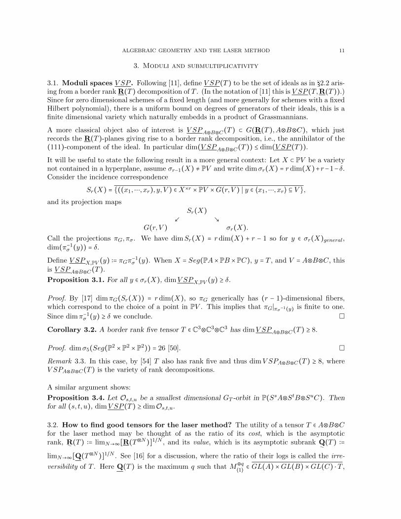
It will be useful to state the following result in a more general context: Let X ⊂ PV be a varietynot contained in a hyperplane, assume σr−1(X) ≠ PV and write dimσr(X) = r dim(X)+r−1−δ.Consider the incidence correspondence

Sr(X) = ((x1,⋯, xr), y, V ) ∈X×r × PV ×G(r, V ) ∣ y ∈ ⟨x1,⋯, xr⟩ ⊆ V ,and its projection maps

Sr(X)

G(r, V ) σr(X).Call the projections πG, πσ. We have dimSr(X) = r dim(X) + r − 1 so for y ∈ σr(X)general,dim(π−1

σ (y)) = δ.

Define V SPX,PV (y) ∶= πGπ−1σ (y). When X = Seg(PA×PB ×PC), y = T , and V = A⊗B⊗C, this

is V SPA⊗B⊗C(T ).Proposition 3.1. For all y ∈ σr(X), dimV SPX,PV (y) ≥ δ.

Proof. By [17] dimπG(Sr(X)) = r dim(X), so πG generically has (r − 1)-dimensional fibers,which correspond to the choice of a point in PV . This implies that πG∣πσ−1(y) is finite to one.

Since dimπ−1σ (y) ≥ δ we conclude.

Corollary 3.2. A border rank five tensor T ∈ C3⊗C3⊗C3 has dimV SPA⊗B⊗C(T ) ≥ 8.

Proof. dimσ5(Seg(P2 × P2 × P2)) = 26 [50].

Remark 3.3. In this case, by [54] T also has rank five and thus dimV SPA⊗B⊗C(T ) ≥ 8, whereV SPA⊗B⊗C(T ) is the variety of rank decompositions.

A similar argument shows:

Proposition 3.4. Let Os,t,u be a smallest dimensional GT -orbit in P(SsA⊗StB⊗SuC). Thenfor all (s, t, u), dimV SP (T ) ≥ dimOs,t,u.

3.2. How to find good tensors for the laser method? The utility of a tensor T ∈ A⊗B⊗Cfor the laser method may be thought of as the ratio of its cost, which is the asymptoticrank, R

:(T ) ∶= limN→∞[R(T⊠N)]1/N , and its value, which is its asymptotic subrank Q

:(T ) ∶=

limN→∞[Q(T⊠N)]1/N . See [16] for a discussion, where the ratio of their logs is called the irre-

versibility of T . Here Q(T ) is the maximum q such that M⊕q⟨1⟩

∈ GL(A) ×GL(B) ×GL(C) ⋅ T ,


where M⊕q⟨1⟩

is the so-called unit tensor, in bases M⊕q⟨1⟩

= ∑qj=1 aj⊗bj⊗cj . Unless a tensor is of

minimal border rank, we only can estimate the asymptotic rank of a tensor by computing itsborder rank and the border rank of its small Kronecker powers.

There are several papers attempting to find tensors that give good upper bounds on ω in thelaser method:

Papers on barriers may be interpreted as describing where not to look for good tensors: [16,2, 4, 1] discuss limits of the laser method for various types of tensors and various types ofimplementations.

A program to utilize algebraic geometry and representation theory to find good tensors for thelaser method was initiated in [19, 33].

Here we describe a more modest goal: determine criteria that indicate (or even guarantee) thatborder rank is strictly sub-multiplicative under the Kronecker square.

To our knowledge, the first example of a non-minimal border rank tensor that satisfied R(T⊠2) =R(T )2 was given in [18]: the small Coppersmith-Winograd tensor Tcw,q for q > 2 and in thispaper we show equality also holds when q = 2. This shows that tight tensors need not exhibitstrict submultiplicativity. Several examples of strict submultiplicativity were known previousto this paper: the 2 × 2 matrix multiplication tensor M⟨2⟩ ∈ C4⊗C4⊗C4, R(M⟨2⟩) = 7 [29] while

R(M⊠2⟨2⟩

) ≤ 46 [48]. The tensors of [15] have a drop of one, a generic tensor T ∈ C3⊗C3⊗C3

satisfies R(T ) = 5 while R(T⊠2) ≤ 22 [18], and R(Tskewcw,2) = 5 while R(T⊠2skewcw,2) = 17 [18, 20].

3.3. V SP and strict submultiplicativity. All the strict submultiplicativity examples havepositive dimensional V SP . This is attributable to the degeneracy of σ4(Seg(P2 × P2 × P2)) forthe generic tensors in C3⊗C3⊗C3, and to the large symmetry groups for the other cases: If atensor T ∈ A⊗B⊗C has a positive dimensional symmetry group GT and GT does not have aone-dimensional submodule in each of A⊗B, A⊗C, B⊗C, A⊗B⊗C, then dim(V SP (T )) > 0because any ideal in the GT -orbit closure of an ideal of a border rank decomposition for T willgive another border rank decomposition.

It would be too much to hope that a concise tensor T not of minimal border rank satisfyingdimV SP (T ) > 0 also satisfies R(T⊠2) < R(T )2. Consider the following example: Let T = T1⊕T2

with the Tj in disjoint spaces, where T1 has non-minimal border rank and dimV SP (T1) = 0and T2 has minimal border rank with dimV SP (T2) > 0. Then there is no reason to believe T⊠2

should have strict submultiplicativity.

It is possible that the converse holds: that strict submultiplicativity under the Kronecker squareimplies a positive dimensional V SP .

It might be useful, following [15] to split the submultiplicativity question into two questions: firstto determine if the usual tensor square is submultiplicative and then if the border rank of theKronecker square is less than the border rank of the tensor square. Note that in general, assumingnon-defectivity, for a projective variety X ⊂ PV of dimension N , σR−1(X) has codimensionN + 1 in σR(X). In our case R = r2 and in the tensor square case N = 6m − 6, and in theKronecker square case N = 3m2 − 3. A priori, for T ∈ Cm⊗Cm⊗Cm of border rank r, T⊗2 ∈σr2(Seg(P(m−1)×6)) and submultiplicativity is a codimension 6m − 5 condition, whereas T⊠2 ∈σr2(Seg(P(m

2−1)×3)) and submultiplicativity is a codimension 3m2 − 2 condition. Despite this,the second condition is weaker than the first.


4. Koszul flattening lower bounds

The best general technique available for border rank lower bounds are Koszul flattenings [37, 35].

Fix an integer p. Given a tensor T = ∑ijk T ijkai⊗ bj ⊗ ck ∈ A⊗B⊗C, the p-th Koszul flatteningof T on the space A is the linear map

T∧pA ∶ ΛpA⊗B∗ → Λp+1A⊗C

X⊗β ↦ ∑ijkT ijkβ(bj)(ai ∧X)⊗ck.

Then [35, Proposition 4.1.1] states

(6) R(T ) ≥rank(T ∧pA )(dim(A)−1

p).

The best lower bounds for any given p are obtained by restricting T to a generic 2p+1 dimensionalsubspace of A∗ so the denominator becomes (2p

p).

Theorem 4.1. The following border rank lower bounds are obtained by applying Koszul flat-tenings to a restriction of the tensor to a sufficiently generic C2p+1⊗B⊗C ⊂ A⊗B⊗C. Values ofp that give the bound are in parentheses.

(1) R(T⊠2skewcw,4) ≥ 39 (p = 2,3,4)

(2) R(T⊠2skewcw,6) ≥ 70 (p = 2,3,4)

(3) R(T⊠2skewcw,8) ≥ 110 (p = 4)

(4) R(T⊠2skewcw,10) ≥ 157 (p = 4)

(5) R(T⊠3skewcw,2) ≥ 49 (p = 4)

(6) R(T⊠3skewcw,4) ≥ 219 (p = 3)

(7) R(T⊠3skewcw,6) ≥ 550 (p = 3)

(8) R(T⊠3skewcw,8) ≥ 1089 (p = 3)

(9) R(T⊠3skewcw,10) ≥ 1886 (p = 3).

Better lower bounds for the larger cases are potentially possible, if not easily accessible, usinglarger values of p.

Compare these with the values for the small Coppersmith-Winograd tensor from [18]:

(1) R(T⊠2cw,4) = 36

(2) R(T⊠2cw,6) = 64

(3) R(T⊠2cw,8) = 100

(4) R(T⊠2cw,10) = 144

(5) R(T⊠3cw,4) ≥ 180

(6) R(T⊠3cw,6) = 512


(7) R(T⊠3cw,8) = 1000

(8) R(T⊠3cw,10) = 1728.

Note that R(T⊠4cw,q) ≤ (q + 2)4 and that R(T⊠4

skewcw,q) is at least the estimate in Proposition

4.1 times q + 1 by [18, Prop. 4.2]. Based on this, it is possible as of this writing that ofR(T⊠4

skewcw,q) ≤ R(T⊠4cw,q) for q = 2,6,8.

5. Proof of Theorem 1.1 that R(perm3) = 16

The upper bound follows as R(Tcw,2) = 4.

For the lower bound, we prove there is no E110 ⊂ A⊗B of dimension 15 that satisfies the flagcondition and passes the (210) and (120) tests. To do this, we need to show there is no E′

110

of dimension six that is spanned by weight vectors such that the resulting E110 passes the testsand satisfies the flag condition. We do this by separately analyzing the pure and mixed kernelsdiscussed in §2.5:

Lemma 5.1. There is a unique up to isomorphism choice of six-dimensional BTcw,2-fixed E′110

satisfying the flag condition with κm = 5 and this choice fails the (210)-test. All other choicessatisfy κm, κ

′m ≤ 4.

Lemma 5.2. For any six-dimensional E′110, κp, κ

′p ≤ 10 and if equality holds, then κm, κ

′m < 4.

Lemmas 5.1 and 5.2 together prove Theorem 1.1.

In order to prove Lemma 5.1 we need to analyze what the flag condition imposes on potentialE′

110. It turns out we only need to analyze the first three steps carefully. The essential point iswhen we analyze potential contributions to the mixed kernel, any element of the kernel carriesa “cost” of at least three, in the sense that either three rank one weight vectors are used toconstruct the element of the kernel, or a weight vector that cannot appear until the third stepin a flag is used, or a similar intermediate combination results in a cost of three.

In what follows, i, j, k = 1,2,3, i′, j′, k′ = 1,2,3, k′ ∈ i′, j′, k ∈ i, j etc..

Hereperm3(C∗) = ⟨aii′⊗bii′ + a

ii′⊗bii′ + a

ii′⊗bii′ + aii′⊗b

ii′⟩.

Thus perm3(C∗) ∩ σ3 = ;. Observe that κf = 1 as

(perm3(C∗)⊗A) ∩ (S2A⊗B) = ⟨∑akk′⊗(aii′⊗bjj′ + a

ji′⊗b

ij′ + aij′⊗b

ji′ + a

jj′⊗b

ii′)⟩.

Remark 5.3. In general, for any symmetric tensor T , κf ≥ 1 due to the copy of T in S3A ⊂S2A⊗B.

The possible weights of elements in A⊗B are (200)(200), (110)(110), (200)(110) and theirpermutations under the action of (S3 ×S3) ⋊ Z2. We will say an element has type (xyz)(pqr)if its weight is in the (S3 ×S3) ⋊Z2-orbit of (xyz)(pqr).

First step in flag: rank one weight vectors. All weight vectors of type (200)(200) haverank one, these are of the form aii′⊗bii′ . Vectors of type (200)(110) have rank one or two, thoseof rank one are of the form aii′⊗bik′ and vectors of type (110)(110) have rank at most four, the

rank one vectors among them are of the form aii′⊗bjj′ .


Second step in the flag. Given the first step, we could get the second step either by addinganother rank one weight vector, or taking a tangent vector to a rank one weight vector.

The rank two weight vectors tangent to a rank one element of type (200)(200), which we may

write as ajj′⊗bjj′ , are up to scale ajj′⊗b

j

j′+Kaj

j′⊗bjj′ , for some K ≠ 0, or its Z2-image, which are

of type (200)(110) or ajj′⊗bj

j′+Kaj

j′⊗bjj′ , which are of type (110)(110).

No rank two tangent vector to a rank one element of type (110)(110) is a weight vector.

The rank two tangent weight vectors to a rank one element of type (200)(110), e.g., aii′⊗bik′ , are

of the form aii′⊗bik′ +Kaii′⊗bik′ for some K ≠ 0, and they are of type (110)(110).

Third step in the flag. Given a two-step flag, the third step may be obtained either by addinganother rank one weight vector, or adding a new tangent vector to one of the rank one vectors inthe flag, or taking a rank three second derivative of a weight vector, whose first tangent vectoralso appears in the flag, or by taking a vector of the form x′ +y′ where x, y are rank one, appearin the flag, and are colinear.

Consider rank three second derivatives of a weight vector: Say we had some

(7) (a + ta′ + t2a′′)⊗(b + tb′ + t2b′′) = a⊗b + t(a⊗b′ + a′⊗b) + t2(a⊗b′′ + a′⊗b′ + a′′⊗b) + ...

In order that the t coefficient appears in E′110, either we would need either a′⊗b + a⊗b′ to

be a weight vector, or one of a⊗b′, a′⊗b to be a multiple of a⊗b. The second case yieldsnothing interesting. To see this, assume b′ = λb. Then the coefficient of t2 may be written asa⊗b′′ + (λa′ + a′′)⊗b, which is just a tangent vector to the original point, so we are just in thesituation of a rank one point and two tangent vectors, so we ignore this situation.

Recalling the possible tangent vectors that are weight vectors we have three potential cases:

⟨ajj′⊗bjj′ , a

jj′⊗b

j

j′+Kaj

j′⊗bjj′ , a

jj′⊗b

′′ + ajj′⊗bj

j′+Ka′′⊗bjj′⟩

⟨ajj′⊗bjj′ , a

jj′⊗b

j

j′+Kaj

j′⊗bjj′ , a

′′⊗bjj′+ aj

j′⊗bj

j′+ aj

j′⊗b′′⟩

⟨aii′⊗bik′ , aii′⊗bik′ +Ka

ii′⊗bik′ , a

′′⊗bik′ + aii′⊗bik′ +Ka

ii′⊗b′′⟩

In the first case, the third vector is not a weight vector for any choice of a′′, b′′ not both zero,and in the other two cases the third vector can only be a weight vector if the third term collapsesto a rank one element, and thus this scenario does not occur.

Since no two vectors of type (200)(200) are colinear, the only possibility of a vector of the formx′ + y′ appearing is if x is of type (200)(200) and y of type (200)(110), but in this case one justgets a weight vector of the form x′ of type (110)(110) by the weight vector requirement. If x, yare of type (200)(110), then any nontrivial x′ + y′ is not a weight vector. Thus this scenariodoes not occur.

Proof of Lemma 5.1. We first describe all possible elements in the mixed kernel, these are givenin equations (8) - (18). We then show that with a 6-dimensional E′

110 satisfying the flag condition,no matter what combinations appear, there is at most a four dimensional contribution to themixed kernel, with a unique (up to symmetry) exception whose pure kernel is too small for it topass the (210) test.


Let Γ = Z2 ×Z2 and Γ ⋅ ajj′⊗bkk′ = a

jj′⊗b

kk′ + a

jk′⊗b

kj′ + akj′⊗b

jk′ + a

kk′⊗b

jj′ . In what follows underlined

terms are elements of E′110. The group Gperm3

allows us to unambiguously define the elementsof E′

110 except those of type (110)(110).

Up to (S3 ×S3) ⋊ Z2, there are four types of potential vectors in the mixed kernel that use a

single element Γ ⋅ aii′⊗bjj′ of perm3(C∗):

First, E′110 could contain a complement to Γ ⋅aii′⊗b

jj′ in its weight space (the complement is three

dimensional). We have the following types:

(8) ajj′⊗(Γ ⋅ aii′⊗bjj′) − a

jj′⊗(aii′⊗b

jj′) − a

jj′⊗(aij′⊗b

ji′) − a

jj′⊗(aji′⊗b

ij′),

(9) ajj′⊗(Γ ⋅ aii′⊗bjj′) − a

jj′⊗(aii′⊗b

jj′ + a

ij′⊗b

ji′) − a

jj′⊗(aji′⊗b

ij′),

(10) ajj′⊗(Γ ⋅ aii′⊗bjj′) − a

jj′⊗(aji′⊗b

ij′ + aij′⊗b

ji′) − a

jj′⊗(aii′⊗b

jj′),

(11) ajj′⊗(Γ ⋅ aii′⊗bjj′) − a

jj′⊗(aii′⊗b

jj′ + a

ij′⊗b

ji′ + a

ji′⊗b

ij′).

We distinguish (9) and (10) because in (10) the rank two element appearing is tangent to a rankone weight vector of type (200)(200) and this is not the case in (9).

Note that the flag condition is crucial here: otherwise we could just take six vectors of the typeappearing in (11) to have κm = 6.

The other potential elements of the mixed kernel utilizing a single element of perm3(C∗) are(here and below, K,K ′ are constants):

(12) ajj′⊗(Γ ⋅ ajj′⊗bjj′) + a

j

j′⊗(ajj′⊗b

jj′) + a

jj′⊗(ajj′⊗b

j

j′+Kaj

j′⊗bjj′) + a

j

j′⊗(ajj′⊗b

jj′ +Ka

jj′⊗b

jj′),

where the underlined terms are respectively types (200)(200), (200)(110), (200)(110),

aii′⊗(Γ ⋅ akk′⊗bjj′) + a

kk′⊗(aii′⊗b

jj′ +Ka

jj′⊗b

ii′) + akj′⊗(aii′⊗b

jk′ +K

′ajk′⊗bii′)(13)

+ ajk′⊗(aii′⊗bkj′ +K ′akj′⊗bii′) + ajj′⊗(aii′⊗bkk′ +Ka

kk′⊗b

ii′),

where the underlined terms are all of type (110)(110) and they all live in different weight spaces,and

aji′⊗(Γ ⋅ ajk′⊗bjj′) + a

jk′⊗(aji′⊗b

jj′ +Ka

jj′⊗b

ji′) + a

jj′⊗(aji′⊗b

jk′ +K

′ajk′⊗bji′)(14)

+ ajk′⊗(aji′⊗bjj′ +K

′ajj′⊗bji′) + a

jj′⊗(aji′⊗b

jk′ +Ka

jk′⊗b

ji′),

where the underlined terms are respectively of types (200)(110), (200)(110), (110)(110), (110)(110).The two elements of type (110)(110) live in different weight spaces.

The possible terms in the mixed kernel with two elements of perm3(C∗) that are not just sumsof terms with one element having no cancellation are as follows:


aii⊗(Γ ⋅ akk⊗bij) + aik⊗(Γ ⋅ aii⊗bkj )

(15)

+ akk⊗(aii⊗bij +Kaij⊗bii) + akj⊗(aii⊗bik + aik⊗b

ii) + aki⊗(aik⊗b

ij) + aij⊗(aii⊗bkk +Ka

kk⊗b

ii) + aij⊗(aik⊗b

ki ),

where the underlined terms are respectively of types (200)(110), (200)(110), (200)(110), (110)(110),(110)(110) and the two type (110)(110) vectors live in different weight spaces, and

aii⊗(Γ ⋅ akk⊗bij) + aij⊗(Γ ⋅ aii⊗bkk)

(16)

+ akk⊗(aii⊗bij + aij⊗bii) + akj⊗(aii⊗bik +K′aik⊗b

ii) + aik⊗(aii⊗bkj +K ′akj⊗bii) + aik⊗(aij⊗bki ) + aki⊗(aij⊗bik),

where the underlined terms are respectively of types (200)(110), (200)(110), (110)(110), (110)(110)and the two type (110)(110) vectors live in different weight spaces.

The possible terms in the mixed kernel with three elements of perm3(C∗) are:

aii′⊗(Γ ⋅ aik′⊗bij′) + aik′⊗(Γ ⋅ aii′⊗bij′) + aij′⊗(Γ ⋅ aii′⊗bik′)(17)

+ aik′⊗(aii′⊗bij′ + aij′⊗bii′) + aij′⊗(aii′⊗bik′ + aik′⊗b

ii′) + aii′⊗(aik′⊗b

ij′ + aij′⊗bik′),

where all have type (200)(110), with the same (200) weight space and the three distinct (110)weight spaces.

aii′⊗(Γ ⋅ ajj′⊗bkk′) + a

jj′⊗(Γ ⋅ aii′⊗bkk′) + a

kk′⊗(Γ ⋅ aii′⊗b

jj′)(18)

+ aii′⊗(ajk′⊗bkj′ + akj′⊗b

jk′) + a

jj′⊗(aik′⊗b

ki′ + aki′⊗bii′) + akk′⊗(aij′⊗b

ji′ + a

ji′⊗b

ij′),

where all have type (110)(110) and lie in different weight spaces.

We first observe that no element appears in more than 4 of the potential kernel vectors. Sincewe only have six elements to obtain a 5 dimensional mixed kernel, we see any potential kernelvector using more than 3 elements of E′

110 cannot be used. (Here we are also using that withvectors involving more than 3 elements, no pair of elements appears in a same second potentialkernel vector.) We are reduced to examining (8), (9), (11), (12), (17) and (18).

Case: the kernel contains an element of type (8). We have three elements of type (110)(110) allof the same weight in E′

110. The only other relations among those we consider that use elementsof type (110)(110) are of type (18), but this requires two additional elements of that type withdifferent weights. We conclude elements of type (8) will not be useful.

Case: the kernel contains an element of type (9) or (10). The second underlined term is nottangent to the first, so the cost of such an element is three. If the element is obtained naively,we are in the same situtation as (8). For case (10) there is also the possibility to obtain the ranktwo element as a tangent vector to an element of type (200)(200). If we form the 3-plane withthe (200)(200) vector and want to use it in some other relation, we cannot reuse the (110)(110)vectors with it as no other kernel element involves this mixture of weights, so these cases arenot useful.


Case: the kernel contains an element of type (11). We have seen there is no way to constructthe element appearing at cost three other than as the sum of three rank one elements or as thesum of a rank one element and a tangent vector as above. Thus this case reduces to one of theprevious two cases.

Case: the kernel contains an element of type (12). These use an element of type (200)(200)and two of its type (200)(110) tangent vectors. Each (200)(200) element appears in 4 relations

of type (12). To obtain them, we only need include the four vectors ajj′⊗bj

j′+ aj

j′⊗bjj′ , a

jj′⊗b

jj′ +

Kajj′⊗bjj′ (where there are two possibilities for each of the the two hatted vectors). When K = 1,

this gives κm, κ′m = 4 (if K ≠ 1, then κ′m is smaller). At this point we have a five-plane in E′

110.We could take a (200)(110)-vector appearing as a tangent vector to the (200)(200) vector andattempt to use it in an element of type (17), in fact we may use two tangent vectors in such anexpression, but we still need to add a third (200)(110) vector that is not of rank one, and is nottangent to the (200)(200) vector. Explicitly, we may take

(19) E′110 = ⟨a1

1⊗b11, a11⊗b12 + a1

2⊗b11, a11⊗b13 + a1

3⊗b11, a11⊗b21 + a2

1⊗b11, a11⊗b31 + a3

1⊗b11, a12⊗b13 + a1

3⊗b12⟩

Here the (210) test fails, κp = 6 (for each basis vector v of E′110 there is a pure kernel of the form

a11⊗v +⋯), so the total kernel has dimension 12.

Case: the kernel contains an element of type (17). Each element is a tangent vector to a samevector of type (200)(200), namely aii′⊗bii′ . Thus to get just one element of the kernel alreadyuses 4 dimensions of E′

110. Unless we enlarge to obtain (19), we would have to enlarge to obtaineither additional relations of type (17) or relations of type (18). To get a second such relation,one needs at least two more elements, which would fill E′

110 and only give κm = 3. The terms in(18) have a different type, so that will not work either.

Case: the kernel contains an element of type (18). The elements appearing are all of type(110)(110) and in different weight spaces so at most one of these could be re-used in a differentrelation, so this situation cannot occur.

For the proof of Lemma 5.2 we use a basic fact from exterior differential systems (the easy partof Cartan’s test) [28, Prop. 4.5.3]: let B1 ⊂ B2 ⊂ ⋯ ⊂ B9 be a generic flag in B (generic inthe sense that s1 below is maximized, and having maximized s1, s2 is maximized etc..). Let s1

be the dimension of the projection of E′110 to A⊗B1. Define s2 by s1 + s2 is dimension of the

projection of E′110 to A⊗B2, set s1 + s2 + s3 to be the dimension of E′

110 projected to A⊗B3 etc..Then

(20) dim(S2A⊗B) ∩ (A⊗E′110) ≤ s1 + 2s2 +⋯ + 6s6.

In particular, κp ≤ s1 + 2s2 +⋯ + 6s6. If equality holds in (20), we will say E′110 is A-involutive.

Proof of Lemma 5.2. Let t1,⋯, t6 be the corresponding quantities for the (120) test. The onlyway to have κp, κ

′p ≥ 10 is if the associated Young diagrams are respectively A and B involutive,

and both the staircase, i.e., s1 = t1 = 3, s2 = t2 = 2, s3 = t3 = 1. This is because involutivitycan only hold if E′

110 is spanned by rank one elements and in this case the B-diagram is thetranspose of the A-diagram.

Thus there are a1, a2, a3 ∈ A and b1, b2, b3 ∈ B such that

E′110 = ⟨a1⊗b1, a1⊗b2, a2⊗b1, a1⊗b3, a3⊗b1, a2⊗b2⟩.


The best one can do here is to obtain κm = 1, e.g., by taking a1 = a11, a2 = a1

3, a3 = a31 and

similarly for the bj .

Remark 5.4. The reason perm3 was previously unaccessible was that already to choose E′110,

without the flag condition one needed to introduce numerous parameters due to the high weightmultiplicities that made the calculation infeasible. The flag condition guaranteed the presenceof low rank elements in E′

110 which significantly reduced the search space.

Remark 5.5. It is interesting to see what happens when dimE′110 = 7, to obtain a border rank

16 ideal fixed by the torus in Gperm3. One may take for example

E′110 = ⟨a1

1⊗b11, a12⊗b11 + a1

1⊗b12, a13⊗b11 + a1

1⊗b13, a21⊗b11 + a1

1⊗b21, a31⊗b11 + a1

1⊗b31, a12⊗b12, a1

3⊗b12 + a12⊗b13⟩.

Then we obtain the four (200)(200) contributions to κm from expressions of type (12) as wellas three additional contributions from expressions of type (17). Here s1 = t1 = 4, s2 = t2 = 3 and

(A⊗E′110) ∩ (S2A⊗B) =

⟨a11⊗a1

1⊗b11, a12⊗a1

1⊗b11 + a11⊗(a1

2⊗b11 + a11⊗b12), a1

3⊗a11⊗b11 + a1

1⊗(a13⊗b11 + a1

1⊗b13),a2

1⊗a11⊗b11 + a1

1⊗(a21⊗b11 + a1

1⊗b21), a31⊗a1

1⊗b11 + a11⊗(a3

1⊗b11 + a11⊗b31),

a12⊗a1

2⊗b12, a11⊗a1

2⊗b12 + a12⊗(a1

2⊗b11 + a11⊗b12), a1

3⊗a12⊗b12 + a1

2⊗(a13⊗b12 + a1

2⊗b13)⟩

so κp = κ′p = 8 and both the (210) and (120) tests are passed.

6. Descriptions of V SP (Tcw,q)

In this section we adopt the index range 1 ≤ α,β ≤ q. The small Coppersmith-Winograd tensorhas a well-known border rank decomposition, which is also a Waring border rank decomposition.

Tcw,q = limt→0

1

t2∑α

[(a0 + taα)⊗(b0 + tbα)⊗(c0 + tcα)]

− 1

t3[(a0 + t2∑

α

aα)⊗(b0 + t2∑α

bα)⊗(c0 + t2∑α

cα)]

− (q 1

t2− 1

t3)a0⊗b0⊗c0.

Let q > 2. Write A = B = C = L ⊕M , where L = ⟨a0⟩ and M = ⟨aα⟩. Set Q = ∑α aα⊗aα. Astraight-forward Lie algebra calculation (see, e.g., [19]) shows GTcw,q ⊃ SO(M,Q) × GL(L) =SO(q) ×C∗. Then

A⊗B = L⊗2 ⊕L ∧M ⊕ S20M ⊕Λ2M ⊕ (L ⋅M ⊕Q),

where the term in parenthesis is Tcw,q(C∗). Here S20M =M2ω1 is the complement to the trivial

SO(M,Q)-representation in S2M . In what follows we write Lk for L⊗k = SkL.

Theorem 6.1. For q > 2, V SP (Tcw,q) is a point. The unique ideal is as follows: for all s, t, uwith s + t + u = d, the annhilator of the ideal in degree (s, t, u) is

Ld ⊕Ld−1 ⋅M ⊕Ld−2 ⋅Q.Here

Ld−1 ⋅M = ⟨as−10 ⋅ aα⊗bt0⊗cu0 + as0⊗bt−1

0 ⋅ bα⊗cu0 + as0⊗bt0⊗cu−10 ⋅ cα ∣ α = 1,⋯, q⟩


and

Ld−2 ⋅Q = ⟨∑α

as−10 ⋅ aα⊗bt−1

0 ⋅ bα⊗cu0 + as−10 ⋅ aα⊗bt0⊗cu−1

0 ⋅ cα + as0⊗bt−10 ⋅ bα⊗cu−1

0 ⋅ cα

+ as−20 ⋅ a2

α⊗bt0⊗cu0 + as0⊗bt−20 ⋅ b2α⊗cu−1

0 ⋅ cα + as0⊗bt0⊗cu−20 ⋅ c2

α⟩.

Proof. We must have PE110 ∩ Seg(PA × PB) ≠ ;. This may be achieved by adding some

(u0a0 +∑α

uαaα)⊗(v0b0 +∑β

vβbβ)

for u0, uα, v0, vβ ∈ C. We also must have a flag as in Observation 2.5. Taking anything other thana0⊗b0, (u0a0+a)⊗b0 with u0 ∈ C, a ∈M , or xa0⊗bα+yaα⊗b0 (i.e., some a0⊗bα or aα⊗b0 since weare working modulo T (C∗)) makes the flag condition PF2 ⊂ σ2(Seg(PA×PB)) fail. (Here we usethat q > 2.) Taking anything other than a0⊗b0 makes the flag condition PF3 ⊂ σ3(Seg(PA×PB))fail. Thus there is a unique E110, and by symmetry unique E101 and E011. This triple exactlypasses all degree three tests.

To see E200 must be as asserted, it must be such that (E200⊗B) ⊇ E210. In order to have L⊗3

in this intersection, we need L⊗2 ⊂ E200. In order to have L2 ⋅M = ⟨a0⊗a0⊗bα + a0⊗aα⊗b0 +aα⊗a0⊗b0⟩ in the intersection, we see it must also contain ⟨a0⊗aα + aα⊗a0⟩ = L ⋅M . In order tohave L ⋅Q = ⟨∑α(a0⊗aα⊗bα + aα⊗a0⊗bα + aα⊗aα⊗b0)⟩ in the intersection, we see it must alsocontain ⟨∑α aα⊗aα⟩ = Q.

For the general case, assume by induction Es−1,t,u,Es,t−1,u,Es,t,u−1 are as asserted and isomorphic

as a module to L⊗d−1⊕Ld−2 ⋅M ⊕Ld−3 ⋅Q. Arguing as we did for E200, first obtaining L⊗d, thenLd−1 ⋅M , then Ld−2 ⋅Q we conclude.

Note that the ideal is GTcw,q -fixed as indeed it has to be if V SP is a point.

Now let q = 2, in this case it is more convenient to write Tcw,2 as

Tcw,2 = ∑σ∈S3

aσ(1)⊗bσ(2)⊗cσ(3).

Write A = B = C = L1 ⊕ L2 ⊕ L3 where, e.g., for A, Lj = ⟨aj⟩. A straight-forward Lie algebra

calculation shows GTcw,2 ⊇ (C∗)×3.

Theorem 6.2. V SP (Tcw,2) and V SP v3(P2),PS3C3(Tcw,2) each consists of three points. One

choice has for all s, t, u with s + t + u = d, the annihilator in degree (s, t, u) equal to

Ls1⊗Lt1⊗Lu1 ⊕ φ(Ld−11 ⊗L2)⊕ φ(Ld−1

1 ⊗L3)⊕ φ(Ls−21 ⊗L2⊗L3)

where φ ∶ (Ld−11 ⊗Lx) → SsA⊗StB⊗SuC is the symmetric embedding. The other two choices

arise from exchanging the role of L1 with L2, L3.

Proof. We have Tcw,2(C∗) = ⟨ai⊗bj + bj⊗ai ∣ i ≠ j⟩. The only possibilites for E110 for r = 4 thatpass the (210)-test arise by adding ak⊗bk to this for some k ∈ 1,2,3. Take k = 1. Then

(E110⊗A) ∩ (S2A⊗B) = ⟨a21⊗b1, a1a2⊗b1 + a2

1⊗b2, a1a3⊗b1 + a21⊗b3, ∑

σ∈S3

aσ(1)⊗aσ(2)⊗bσ(e)⟩

The only compatible choice of E200 is ⟨a21, a1a2, a1a3, a2a3⟩. The situation for higher multi-

degrees is similar.


Remark 6.3. In contrast to Tcw,2, by Corollary 3.2, dimV SP (Tskewcw,2) ≥ 8. From [23] (slightlychanging notation) we have the rank five decomposition:

Tskewcw,2 =1

2[2a1⊗(b2 − b3)⊗(c2 + c3)

− (a1 + a2)⊗(b1 − b3)⊗(c1 + c3) − (a1 − a2)⊗(b1 + b3)⊗(c1 − c3)+ (a1 + a3)⊗(b1 − b2)⊗(c1 + c2) − (a1 − a3)⊗(b1 + b2)⊗(c1 − c2)]

and the orbit of this decomposition already has dimension 8. (This can be seen by noting thatmore than four distinct vectors in C3 appear in the decomposition.)

7. Tskewcw,q, q > 2

Proof of Theorem 1.3. For the upper bound, we have

Tskewcw,q = limt→0

1

t3[∑ξ

[(a0 + t2aξ)⊗(b0 − t2bξ)⊗(c0 − tcξ+p) + (a0 − t2aξ)⊗(b0 − tbξ+p)⊗(c0 + t2cξ)

(21)

+ (a0 − taξ+p)⊗(b0 + t2bξ)⊗(c0 − t2cξ)]

+ 1

t5(a0 + t3∑

ξ

aξ+p)⊗(b0 + t3∑ξ

bξ+p)⊗(c0 + t3∑ξ

cξ+p)

− ( 3q

2t2+ 1

t5)a0⊗b0⊗c0].

For the lower bounds, write A = B = C = L⊕M with dimL = 1, dimM = q and M is equippedwith a symplectic form Ω. A straight-forward Lie algebra calculation shows GTskewcw,q ⊇ Sp(M)×GL(L) ×M∗⊗L. Then

A⊗B = L⊗2 ⊕L ⋅M ⊕ S2M ⊕Λ2M0 ⊕ (L ∧M ⊕Ω)where the term in parentheses equals Tskewcw,q(C∗). Here Λ2M0 =Mω2 , the complement to the

Sp(M)-trivial representation in Λ2M .

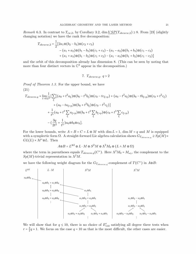
we have the following weight diagram for the GTskewcw,q -complement of T (C∗) in A⊗B:

L⊗2 L ⋅M S2M Λ2M

a0⊗b0a0⊗b1 + a1⊗b0

a0⊗b2 + a2⊗b0

a0⊗b3 + a3⊗b0⋮

a1⊗b1

a1⊗b2 + a2⊗b1

a1⊗b3 + a3⊗b1

a2⊗b3 + a3⊗b2 a1⊗b4 + a4⊗b1⋮

a1⊗b2 − a2⊗b1

a1⊗b3 − a3⊗b1

a2⊗b3 − a3⊗b2 a1⊗b4 − a4⊗b1⋮

We will show that for q ≤ 10, there is no choice of E′110 satisfying all degree three tests when

r = 32q + 1. We focus on the case q = 10 as that is the most difficult, the other cases are easier.


Note that elements of M may be raised to L, so an element of S2M cannot be placed in E′110

unless its raising to L ⋅M is also there. On the other hand, since L ∧M ⊂ E110, there is nosimilar restriction on elements of Λ2M .

We now restrict to q = 10. We split the types of (110) spaces into 10 types of cases dependingon the dimension of E′

110 intersected with the various irreducible modules:

case L⊗2 L ⋅M S2M Λ20M

1 1 4 0 02 1 3 1 03 1 2 2 0

4x 1 2 1 + 12

12

5 0 0 0 56 1 0 0 47 1 1 0 38 1 2 0 29 1 1 1 210 1 2 1 1

Types 1,2,3,8,9,10 are all single cases Types 5,6,7 each involve a choice of subset of weightvectors in Λ2

0M (so they are each a collection of a finite number of cases) and case 4 involves aparameter, where we use 1

2 to indicate the parameter, as the weight vector is a sum of a vectorin the two indicated spaces. Explicitly, case 4x may be written

E′110 = ⟨a0⊗b0, a0⊗b1 + a1⊗b0, a0⊗b2 + a2⊗b0, a1⊗b1, x(a1⊗b2 + a2⊗b1) + a1⊗b2 − a2⊗b⟩.

Of these cases 1,2,3,4x,8,10 pass the (210) and (120) tests. No triple passes the (111) test.

We remark that the decomposition (21) is Z3-invariant.

Corollary 7.1. For 10 ≥ q > 2, and q = 2p even, V SP (Tskewcw,q) contains the isotropic Grass-

mannian GΩ( q2 ,M). In particular it has dimension at least (p2).

Proof. Examining (21), by Sp(M) ⊂ GTskewcw,q we may replace ⟨aξ⟩ with any isotropic subspaceas long as we replace ⟨aξ+p⟩ with the corresponding dual subspace and the same changes inB,C.

8. A simpler Waring border rank 17 expression for det3

In this section and the next, we present explicit decompositions. The method used to obtainthe decompositions is discussed after the second decomposition at the end of §9.


Set i =√−1 and ζ = e2πi/12. Then det3 = ∑17

s=1m⊗3s (t) + O(t), where the ms are the following

matrices

⎛⎜⎝

ζ6

t50 0

0 ζ6 00 0 t5

⎞⎟⎠

⎛⎜⎝

1t5

0 00 1 00 0 0

⎞⎟⎠

⎛⎜⎝

ζ6

t50 0

0 0 tζ8

0 t4ζ4 0

⎞⎟⎠

⎛⎜⎝

ζ4

t50 0

0 0 tζ6

0 0 0

⎞⎟⎠

⎛⎜⎝

ζ5

t50 0

0 0 00 t4 0

⎞⎟⎠

⎛⎜⎝

ζ3

t50 0

0 0 00 0 t5

⎞⎟⎠

⎛⎜⎝

0 ζ10

t4ζ8

t3

0 0 tζ8

t3ζ6 0 0

⎞⎟⎠

⎛⎜⎝

0 ζ8

t4ζ6

t3

0 0 tζ6

0 0 0

⎞⎟⎠

⎛⎜⎝

0 1t4

1t3

0 0 0t3ζ6 0 0

⎞⎟⎠

⎛⎜⎜⎝

0 ζ6

t40

ζ6

t 0 00 0 t5ζ6

⎞⎟⎟⎠

⎛⎜⎝

0 ζ11

t40

0 0 0t3 0 0

⎞⎟⎠

⎛⎜⎝

0 ζ9

t40

0 0 00 0 t5ζ6

⎞⎟⎠

⎛⎜⎜⎝

0 0 1t3

ζ6

t 0 00 t4ζ6 0

⎞⎟⎟⎠

⎛⎜⎝

0 0 1t3

0 ζ4 0t3ζ2 t4 0

⎞⎟⎠

⎛⎜⎝

0 0 ζ6

t3

0 ζ10 00 0 0

⎞⎟⎠

⎛⎜⎜⎜⎜⎝

0 556 ζ2

5t4(1+ 2

5

√5)

13 ζ2

t3

(1− 25

√5)

13 ζ8

t 0 00 0 0

⎞⎟⎟⎟⎟⎠

⎛⎜⎜⎜⎜⎝

0 556 ζ8

5t4(1− 2

5

√5)

13 ζ2

t3

(1+ 25

√5)

13 ζ8

t 0 00 0 0

⎞⎟⎟⎟⎟⎠

.

9. A numerical border rank 42 expression for T⊠2skewcw,4

What follows is an expression for T⊠2skewcw,4 as ∑42

s=1ms(t)⊗3 +O(t) that is satisfied to an error of

at most 4.4 × 10−15 in each entry. Code to verify the assertion is available athttps://www.math.tamu.edu/∼jml/chllasersupp.html.

It consists of 42 matrices whose entries are rational expressions in the following 36 complexnumbers: Let i =

√−1 and let ζ = e2πi/12. Set

z0 = −0.8660155098072051 + 0.9452855522785384i z1 = −1.2981710770246242 + 0.0008968724089185688iz2 = 2.9260271139931078 + 0.1853833642730014i z3 = 0.2542517122150322 + 0.30793819438378284iz4 = 0.6964375578992822 + 0.2772662627986198i z5 = 0.5507020325318998 − 0.0493931308002328iz6 = 1.149228383831849 − 1.1683147648642283i z7 = 0.6586404058476252 − 0.16578044112199047iz8 = 0.7654345273805864 − 0.06877274843008892i z9 = 0.544690883860558 + 0.09720573163212605iz10 = 0.6932236636741451 + 0.14980159446358277i z11 = 0.5862637032385472 − 0.12844523449559558iz12 = 2.384363992555291 − 0.08927102369428247i z13 = 0.9664252976479286 + 0.08480470055107503iz14 = 0.6190926897383283 + 0.15631000400545272i z15 = 0.6283592253932955 − 0.5626050553495663iz16 = 1.8190778570602204 − 0.22163457440913656i z17 = 1.153187286528645 − 0.07977233251120702iz18 = 1.4498877801613976 − 0.22515738202335905i z19 = 0.7262464450114047 + 0.7050051641972112iz20 = 1.1195537528292199 − 0.26381000320340176i z21 = 0.4400325048210471 + 0.6593492930106759iz22 = 0.3476654993676339 + 0.4095417606798612i z23 = 0.9459769225333798 + 0.24589162882727128iz24 = 0.7637135867709066 − 0.10529269213820387i z25 = 0.7409392923310902 − 0.10474756303325146iz26 = 1.0112068238001992 − 0.12695675940574122i z27 = 1.5005677845016696 − 0.24533651960180036iz28 = 0.6134145054919202 + 0.08121891266185506i z29 = 1.145625294745251 − 0.3813562005184122iz30 = 1.0607612533915372 − 0.016294891090460426i z31 = 0.941339345482511 + 0.20413704882122435iz32 = 0.622575977639622 + 0.2555810563389569i z33 = 0.951746321194872 − 0.2894768358835511iz34 = 1.0532801812660977 − 0.2502246606675517i z35 = 1.0207644184200035 − 0.2106937666100475i.


The 42 matrices are:

⎛⎜⎜⎜⎜⎜⎜⎜⎜⎜⎜⎝

ζ3z25z26z31z35t269

ζ8z28t61

z23z25z26z31z33z34

ζ10z24z35t13

z23z25z26z31z33z340 0

z25z26z31z33z35t104

0 0 0ζ9z18z26z32t

148

z21z23z33z235

0 0 0 0 0

0 0ζ7z35t

121

z23z25z226z31z33z34

0ζ8z23z34t

91

z24z235

0 0 0 0 0

⎞⎟⎟⎟⎟⎟⎟⎟⎟⎟⎟⎠

⎛⎜⎜⎜⎜⎜⎜⎜⎜⎜⎜⎜⎝

ζ10z30t269

0ζ10z24z35t

13

z27z28z30z330 0

0 0ζ7z24z35t

178

z27z28z300 0

0 0 0 0 0

0 0ζ6z27z28z

235t

121

z223z25z

226z31z33z

234

0 0

0 ζt184

z27z30z340 0 0

⎞⎟⎟⎟⎟⎟⎟⎟⎟⎟⎟⎟⎠

⎛⎜⎜⎜⎜⎜⎜⎜⎜⎜⎝

0 0 0 0 00 0 0 0 0

0z18z24z28z32t

211

z21z223z25z

333z35

z0t163 0

ζz34t133

z25

0 0 0 0 0ζz23z25z33z24z31t

146ζ5z31z35t

184

z23z227z28z30z

234

0 0 0

⎞⎟⎟⎟⎟⎟⎟⎟⎟⎟⎠

⎛⎜⎜⎜⎜⎜⎜⎜⎜⎜⎝

ζ9z30z27t

269 0 0 ζ7

t650

0 0 0 0 00 0 0 0 0

0ζ5z27t

169

z30z330 0 0

0ζ9z27t

184

z30z34

z28t136

z26z34z350 0

⎞⎟⎟⎟⎟⎟⎟⎟⎟⎟⎠

⎛⎜⎜⎜⎜⎜⎜⎜⎜⎜⎜⎝

ζ4z19z35z3z12z13z18z32t

269 0 0 0ζ4z18z21z34

z2z12z25z31z32z35t17

ζz19z33z35z3z12z13z18z32t

104 0 0 0ζ9z19z26z

232z33z35t

148

z3z12z13z18

0 0 0 0 0ζ4z2z3z13z31

z12z19z20z21z32z34t161 0 0 0 0

0 0 0 0 0

⎞⎟⎟⎟⎟⎟⎟⎟⎟⎟⎟⎠

⎛⎜⎜⎜⎜⎜⎜⎜⎝

1z34t

269 0 0ζz24z26z35z28z34t

65 0

0 0 0 0 0ζ5

t1190 0

z24z26z35t85

z280

0 0 0 0 00 0 0 0 0

⎞⎟⎟⎟⎟⎟⎟⎟⎠

⎛⎜⎜⎜⎜⎜⎜⎜⎜⎜⎜⎜⎝

0ζ2z15z18z19z28z32t

61

z21z23z25z31z233z34

ζ11z15z19z35t13

z340 0

0 0 0 0 00 0 0 0 0

ζ11z15z21z23z25z31z35z18z

219z26z32z34t

161 0 0 0 0

ζ9z21z23z25z33z34z215z18z

219z26z

231z32z

235t146

0 0 0 0

⎞⎟⎟⎟⎟⎟⎟⎟⎟⎟⎟⎟⎠

⎛⎜⎜⎜⎜⎜⎜⎜⎜⎜⎜⎜⎜⎝

ζ5z25z31z23z34t

269 0 0 0 ζ4

t17

0 0 0 0 0ζ10z25z31z23t

119 0ζ7z23z24z33t

163

z220z31

0 ζ3z34t133

0ζ2z223z28z

234t

169

z225z231z33z35

0 0 0

0 0ζ10z23t

136

z25z310 0

⎞⎟⎟⎟⎟⎟⎟⎟⎟⎟⎟⎟⎟⎠

⎛⎜⎜⎜⎜⎜⎜⎜⎜⎜⎜⎝

ζ11z3z19z12z21z23z25z32t

269 0 0 0ζ10z2z18z21z23z24z34

z12z13z19z20z31z32z35t17

ζ8z3z19z33z12z21z23z25z32t

104 0 0 0ζ4z3z19z26z

232z33t

148

z12z21z23z25

0 0 0 0 0ζ9z13z31z35

z2z3z12z18z24z32z34t161 0 0 0 0

0 0 0 0 0

⎞⎟⎟⎟⎟⎟⎟⎟⎟⎟⎟⎠

⎛⎜⎜⎜⎜⎜⎜⎜⎜⎜⎝

ζ9z28t269

0 0 0 0

0 0 0 0 0ζ2z28z34t119

ζ10z34t211

z28z33z350 0 0

0 0 0 0 0

0 0 0ζ5z33z35t

58

z340

⎞⎟⎟⎟⎟⎟⎟⎟⎟⎟⎠

⎛⎜⎜⎜⎜⎜⎜⎜⎜⎜⎜⎜⎝

ζ5z24z26z329z30

z27t269 0

ζ11z322z27z33z35t13

z20z23z28z30z231

ζ2

t650

0 0 0 0 0ζ10z24z26z

329z30z34

z27t119 0 0 ζz34t

85 ζ10z18z322z26z27z32z34z35t

133

z20z21z223z25z28z30

0 0 0 0 0ζ10z18z

322z25z26z27z32z33z35

z20z21z23z24z28z30z31t146

z27t184

z24z26z329z30z34

0 0 0

⎞⎟⎟⎟⎟⎟⎟⎟⎟⎟⎟⎟⎠

⎛⎜⎜⎜⎜⎜⎜⎜⎜⎜⎜⎝

ζ2z25z26z31z32z35z18z21z34t

269

ζ11z21z24z232z35t

61

z25z310 0 0

ζ11z25z26z31z32z33z35z18z21z34t

104 0 0 0ζ11z28t

148

z221z23z24z32z33z34z

335

0 0 0 0 0ζ11z25z31z32z35z18z21z24z34t

161 0 0 0 0

0 0 0 0 0

⎞⎟⎟⎟⎟⎟⎟⎟⎟⎟⎟⎠

⎛⎜⎜⎜⎜⎜⎜⎜⎜⎜⎜⎝

0 0 0 0ζ6z18z26z31z32z20z21z34t

17

0 0 0 0 00 0 0 0 0

ζz221z223z24z25z33

z218z319z20z

226z31z

232t161

0 0 0 0

ζ11

t1460 0 0 0

⎞⎟⎟⎟⎟⎟⎟⎟⎟⎟⎟⎠

⎛⎜⎜⎜⎜⎜⎜⎜⎜⎜⎜⎜⎝

ζ3z9z10z11z18z19z30z32z34z5z7z8z16z21z23z25z33t

269 0 0 0ζz5z11z16z18z24z26z31z32

z4z20z21z25t17

0 0ζ11z5z11z16z20z33t

178

z40 0

0 0 0 0 0ζ10z4

z19z20z27z30z33t161 0 0 0 0

ζ2z4z19z20z27z30z34t

146 0ζ6z9z10z11z18z19z27z28z32t

136

z5z7z8z16z21z23z25z26z33z350 0

⎞⎟⎟⎟⎟⎟⎟⎟⎟⎟⎟⎟⎠

⎛⎜⎜⎜⎜⎜⎜⎜⎜⎜⎝

ζ5z28z235

t2690 0 ζ5

t650

ζ2z28z33z235

t1040 0 ζ8z33t

100 0

0 0 0 0 0

0 0 0 t43 0

0 0 0ζ10z33t

58

z340

⎞⎟⎟⎟⎟⎟⎟⎟⎟⎟⎠

⎛⎜⎜⎜⎜⎜⎜⎜⎜⎜⎜⎜⎝

0ζ9z217z21z24z28z

229t

61

z18z222z25z

227z32z33z34z35

ζ4z22z27t13

z17z26z29z231

ζz22z27z31z33z35z17z28z29t

65 0

0 0 0 0 0

0ζ2z217z21z24z28z

229t

211

z18z222z25z

227z32z33z35

0z22z27z31z33z34z35t

85

z17z28z29

ζ3z18z22z27z32z34t133

z17z21z23z25z29z33

0 0 0 0 0ζ3z18z22z25z27z32z17z21z24z29z31t

146

ζ2z217z22t184

z20z23z24z29z230z31z34

0 0 0

⎞⎟⎟⎟⎟⎟⎟⎟⎟⎟⎟⎟⎠


⎛⎜⎜⎜⎜⎜⎜⎜⎜⎜⎜⎜⎜⎝

ζ11z27z28z230

z26z35t269 0 0 0 ζ3

t17

0 0ζz220z21z25z33t

178

z18z24z26z31z320 0

0 0 0 0 0

0 0ζ7z26z35t

121

z27z28z230z33

0 0

0 0z25z31t

136

z23z26z234

0 0

⎞⎟⎟⎟⎟⎟⎟⎟⎟⎟⎟⎟⎟⎠

⎛⎜⎜⎜⎜⎜⎜⎜⎜⎜⎜⎝

ζ8z25z26z31z32z35z18z21z34t

269 0ζ4z21z24z35t

13

z25z26z31z320 0

ζ5z25z26z31z32z33z35z18z21z34t

104 0 0 0ζ5z28t

148

z221z23z24z32z33z34z

335

0 0 0 0 0ζ5z25z31z32z35z18z21z24z34t

161 0 0 0 0

0 0 0 0 0

⎞⎟⎟⎟⎟⎟⎟⎟⎟⎟⎟⎠

⎛⎜⎜⎜⎜⎜⎜⎜⎜⎜⎜⎜⎜⎝

ζ10z5z18z19z28z30z32z21z23z25z33z35t

269 0 0 0z4z11z16z31z5z19z20t

17

0 0ζ10z4z11z16z20z21z25z33t

178

z5z18z19z24z26z320 0

0 0 0 0 0ζ10z9z10z11z18z24z26z32z34z35

z4z7z8z16z20z21z25z27z28z30z33t161 0 0 0 0

ζ2z9z10z11z18z24z26z32z35z4z7z8z16z20z21z25z27z28z30t

146 0ζz5z18z19z27z

228z32t

136

z21z23z25z26z33z34z235

0 0

⎞⎟⎟⎟⎟⎟⎟⎟⎟⎟⎟⎟⎟⎠

⎛⎜⎜⎜⎜⎜⎜⎜⎜⎜⎜⎜⎝

ζ4z217z22z26z29

z20z23z30z34t269 0

z22z27z28z29z30z234t

13

z17z26z31z35

ζ8z22z24z26z29z33z235

z17z27z228z31z34t

65 0

0 0 0 0 0ζ9z217z22z26z29

z20z23z30t119 0 0

ζ7z22z24z26z29z33z235t

85

z17z27z228z31

ζ11z18z22z27z28z29z30z31z32z334t

133

z17z21z23z25z33z35

0 0 0 0 0ζ11z18z22z25z27z28z29z30z32z

234

z17z21z24z35t146 0 0 0 0

⎞⎟⎟⎟⎟⎟⎟⎟⎟⎟⎟⎟⎠

⎛⎜⎜⎜⎜⎜⎜⎜⎜⎝

0 0 ζ5z19z31t13 0 0

0 0 ζ8z19z31z33t178 0 0

0 0 0 0 0ζ8z21z23z25

z18z219z26z31z32t

161 0 0 0 0z21z23z25z33

z18z219z26z31z32z34t

146 0 0 0 0

⎞⎟⎟⎟⎟⎟⎟⎟⎟⎠

⎛⎜⎜⎜⎜⎜⎜⎜⎝

ζ3

t269ζ7t61

z330 ζ10

t650

z33t104

0 0 ζz33t100 0

0 0 0 0 0ζ4

t1610 0 0 0

0 0 0 0 0

⎞⎟⎟⎟⎟⎟⎟⎟⎠

⎛⎜⎜⎜⎜⎜⎜⎜⎜⎜⎝

0ζ10z216z21z23z25z28t

61

z18z19z32z350

ζ4z18z219z26z31z32z35

z16z21z23z25z28t65 0

0 0 0 0 00 0 0 0 0ζ

z16z19z26z31z33t161 0 0 0 0

ζ5

z16z19z26z31z34t146 0 0 0 0

⎞⎟⎟⎟⎟⎟⎟⎟⎟⎟⎠

⎛⎜⎜⎜⎜⎜⎜⎜⎜⎜⎝

ζ7z28t269

ζ3t61

z28z33z350 0 0

0 0 0 0 0z28z34t119

0 0 0 0

0 ζ4t169

z28z33z350 0 0

0 0 0ζ3z33z35t

58

z340

⎞⎟⎟⎟⎟⎟⎟⎟⎟⎟⎠

⎛⎜⎜⎜⎜⎜⎜⎜⎜⎝

z14t269

ζ4z30t61

z214z27z33

0 0 0

0 0 0 0 00 0 0 0 0

0 0 0ζ11z14z27t

43

z300

0 0 0 0 0

⎞⎟⎟⎟⎟⎟⎟⎟⎟⎠

⎛⎜⎜⎜⎜⎜⎜⎜⎜⎜⎝

ζ10z30t269

ζ2t61

z27z30z330 0 0

0 0 0 0 00 0 0 0 0

0 0ζz35t

121

z26z27z28z30z330

ζz27z28t91

z24z35

0 0 0 0ζ5z27z28z33t

106

z24z34z35

⎞⎟⎟⎟⎟⎟⎟⎟⎟⎟⎠

⎛⎜⎜⎜⎜⎜⎜⎜⎜⎜⎜⎝

ζ4

t269ζ3z28t

61

z33z350 0 0

0 0 0 0 0ζ9z34t119

ζ2z28z34t211

z33z350 0 0

0 0 ζ2t121

z26z330 0

0 0 0 0ζ4z33t

106

z24z34

⎞⎟⎟⎟⎟⎟⎟⎟⎟⎟⎟⎠

⎛⎜⎜⎜⎜⎜⎜⎜⎜⎜⎜⎝

ζ2z14t269

0 0 0 0

0ζ9z30t

226

z214z27

0 0 0

0 0 0 0 0

0ζz30t

169

z214z27z33

0ζz14z27t

43

z300

0 0 0 0 0

⎞⎟⎟⎟⎟⎟⎟⎟⎟⎟⎟⎠

⎛⎜⎜⎜⎜⎜⎜⎜⎜⎜⎜⎝

ζ4z30t269

0ζ4z24z35t

13

z27z28z30z330 0

0 0ζz24z35t

178

z27z28z300 0

0 0 0 0 0

0 0 0 0ζ7z27z28t

91

z24z35

0 0 0 0ζ11z27z28z33t

106

z24z34z35

⎞⎟⎟⎟⎟⎟⎟⎟⎟⎟⎟⎠

⎛⎜⎜⎜⎜⎜⎜⎜⎜⎜⎜⎝

ζ8z18z22z24z26z27z32z20z21z23z31z33t

269 0ζ2z20z22z27z34t

13

z330 0

0 0 0 0 0ζz18z22z24z26z27z32z34z20z21z23z31z33t

119 0ζ3z21z23z24z31t

163

z18z222z26z

227z32

0ζ10z22z27z31z33t

133

z20z23z25

0 0 0 0 0ζ10z22z25z27z

233

z20z24z34t146

ζ3z20z22z35t184

z24z27z28z300 0 0

⎞⎟⎟⎟⎟⎟⎟⎟⎟⎟⎟⎠

⎛⎜⎜⎜⎜⎜⎜⎜⎜⎜⎜⎝

ζ10

t2690 0 0 0

0 0 0 0 0ζ3z34t119

0 0 0 0

0 0 ζ8t121

z26z330 0

0 z1t184 ζ6z25z31t

136

z23z234

0 0

⎞⎟⎟⎟⎟⎟⎟⎟⎟⎟⎟⎠

⎛⎜⎜⎜⎜⎜⎜⎜⎜⎜⎝

ζ5z24z25z33z220z34t

269 0 0 0 ζ8

t17

0 0 0 0 0ζ10z24z25z33

z220t119

0 ζ9t163 0ζ3z23z24z33z34t

133

z220z31

0 0 0 0 0ζ

t1460 0 0 0

⎞⎟⎟⎟⎟⎟⎟⎟⎟⎟⎠


⎛⎜⎜⎜⎜⎜⎜⎜⎜⎜⎝

ζ6

t2690

ζz24t13

z330 0

0 0 0 0 0ζ11z34t119

0z24z34t

163

z330 0

0 0 0 0 0

0 0 0 0ζ6z33t

106

z24z34

⎞⎟⎟⎟⎟⎟⎟⎟⎟⎟⎠

⎛⎜⎜⎜⎜⎜⎜⎜⎜⎜⎜⎝

ζ10z9z34t269

0 0 0 0

0ζz7z8z11z18z31z32z35t

226

z10z21z23z25z27z28z300 0 0

0 0 0 0 0ζ5z9z34t161

0 0 0 0

ζ9z9z33t146

0ζz9z27z28t

136

z26z30z350 0

⎞⎟⎟⎟⎟⎟⎟⎟⎟⎟⎟⎠

⎛⎜⎜⎜⎜⎜⎜⎜⎜⎜⎜⎝

ζ7z21z24z18z23z26z32t

269 0 0 0 ζ5

t17

0 0 0 0 0z21z24z34

z18z23z26z32t119 0 0 0

ζ5z21z24z234t

133

z18z25z26z31z32

0 0 0 0 0ζ8z18z23z25z26z32z33

z220z21z34t

146 0 0 0 0

⎞⎟⎟⎟⎟⎟⎟⎟⎟⎟⎟⎠

⎛⎜⎜⎜⎜⎜⎜⎜⎜⎝

ζ9

t2690 0 ζ4

t650

ζ6z33t104

0 0 ζ7z33t100 0

0 0 0 0 0ζ10

t1610 0 0 0

0 0 0 0 0

⎞⎟⎟⎟⎟⎟⎟⎟⎟⎠

⎛⎜⎜⎜⎜⎜⎜⎜⎜⎜⎜⎜⎝

ζ11z25z35z13t

269 0 0 0ζ7z23z34

z13z31z235t17

ζ8z25z33z35z13t

104 0 0 0ζ4z25z26z

332z33z35t

148

z13

0 0 0 0 0

0ζ11z213z28t

169

z225z33

ζ9z213z31z35t121

z23z25z33z340 0

0 0 0 0 0

⎞⎟⎟⎟⎟⎟⎟⎟⎟⎟⎟⎟⎠

⎛⎜⎜⎜⎜⎜⎜⎜⎜⎜⎜⎝

ζ9z25z26z31z35t269

0 0 0 0

ζ6z25z26z31z33z35t104

0 0 0ζ3z18z26z32t

148

z21z23z33z235

0 0 0 0 0

0 0 0 0ζ2z23z34t

91

z24z235

0 0 0 0 0

⎞⎟⎟⎟⎟⎟⎟⎟⎟⎟⎟⎠

⎛⎜⎜⎜⎜⎜⎜⎜⎜⎜⎜⎜⎝

ζ9z7z11z16z30z34z6z27t

269 0 0ζ11z6z10z21z23z25z26z30

z9z18z32t65 0

0ζ2z8z10z

216z26z28z33z34t

226

z350 0 0

0 0 0 0 0ζ8z8z10z18z32z34

z16z21z23z25z31z33t161 0 0 0 0

z8z10z18z32z16z21z23z25z31t

146 0z7z11z16z28t

136

z6z26z350 0

⎞⎟⎟⎟⎟⎟⎟⎟⎟⎟⎟⎟⎠

⎛⎜⎜⎜⎜⎜⎜⎜⎜⎜⎜⎜⎝

ζ10z6z8z10z26z30z34z27t

269 0 0ζ2z10z16z28z30z6z9z31z35t

65 0

0ζ4z7z11z

216z21z23z25z26z31z33z34t

226

z18z320 0 0

0 0 0 0 0ζ10z7z11z34z35z16z28z33t

161 0 0 0 0

ζ2z7z11z35z16z28t

146 0ζz6z8z10z28t

136

z350 0

⎞⎟⎟⎟⎟⎟⎟⎟⎟⎟⎟⎟⎠

⎛⎜⎜⎜⎜⎜⎜⎜⎜⎜⎜⎜⎝

ζ8

z215z18z21z23t

269ζ3z15z18z28t

61

z23z25z26z31z32z233z34z35

ζ4z15z21z24z32z335t

13

z340 0

ζ5z33z215z18z21z23t

104 0 0 0ζz26z

332z33t

148

z215z18z21z23

0 0 0 0 0ζ11z15z23z25z31z18z21z24z34t

161 0 0 0 0

0 0 0 0 0

⎞⎟⎟⎟⎟⎟⎟⎟⎟⎟⎟⎟⎠

⎛⎜⎜⎜⎜⎜⎜⎜⎜⎜⎜⎜⎜⎝

ζ7z28z235

t269t61

z28z33z235

0 ζ7

t650

ζ4z28z33z235

t1040 0 ζ10z33t

100 0

0 0 0 0 0

0 ζt169

z28z33z235

0 ζ2t43 0

0 0 0z33t

58

z340

⎞⎟⎟⎟⎟⎟⎟⎟⎟⎟⎟⎟⎟⎠

We now give an overview of the method used to obtain the expressions for det3 and T⊠2skewcw,4:

Fix bases ai ∈ A, bi ∈ B, and ci ∈ C. A tensor T ∈ A⊗B⊗C has an expression T = ∑i,j,k T ijkai⊗bj⊗ckand is standard tight in this basis if there exist injective functions ωA ∶ [m] → Z, ωB ∶ [m] → Z,ωC ∶ [m]→ Z so that T ijk ≠ 0 implies ωA(i)+ωB(j)+ωC(k) = 0. In this case, we will call a choiceof (ωA, ωB, ωC) satisfying the constraints a set of tight weights. Given a set of tight weights forT , we consider border rank decompositions of the form:

(22) T = ∑rs=1As(t)⊗Bs(t)⊗Cs(t) +O(t),

where As(t) = ∑mi=1AsitωA(i)ai, Bs(t) = ∑mj=1BsjtωB(j)bj , and Cs(t) = ∑mk=1 CsktωC(k)ck. Notethat when the tight weights are trivial, this is an ordinary rank decomposition. In our situation,the equations correspond to a strict subset of the equations describing a rank decomposition,namely those corresponding to triples (i, j, k) where ωA(i) + ωB(j) + ωC(k) ≤ 0. In the case of

T⊠2skewcw,4 this reduces the number of equations down from (25+2

3) = 2925 to 692 and just as with

a rank decomposition, there are 3rm = 3150 unknowns.


We pick a choice of tight weights which minimizes the number of equations to be solved. Theproblem of obtaining a border rank decomposition is then split into two questions: first, tocompute a set of tight weights (ωA, ωB, ωC) so that #(i, j, k) ∣ ωA(i) + ωB(j) + ωC(k) ≤ 0 isminimal, and second, to solve the resulting equations (22) in the Asi, Bsj , Csk.

Consider the first question. Given sets S≤, S> ⊂ [m]×[m]×[m], consider the problem of decidingif there are tight weights (ωA, ωB, ωC) satisfying the additional constraints that ωA(i)+ωB(j)+ωC(k) ≤ 0 for (i, j, k) ∈ S≤ and ωA(i)+ωB(j)+ωC(k) ≥ 1 for (i, j, k) ∈ S>. These conditions alongwith the original equality conditions form a linear program on the images of (ωA, ωB, ωC) whichmay be efficiently solved. There is no harm in letting the linear program be defined over therationals, as we may clear denominators to obtain a solution in integers. One can use this fact toprune an exhaustive search of choices of S≤, S> to find one for which S≤∪S> = [m]×[m]×[m], thereexists a corresponding set of tight weights, and #S≤ is minimal. While this is an exponentialprocedure, this optimization was sufficient to solve the problem for this decomposition.

The second problem, solving the associated system, is solved with the Levenberg-Marquardtnonlinear least squares algorithm [39, 41]. The sparse structure of the answer is obtained byspeculatively zeroing (or setting to simple values) coefficients until all freedom with respect tothe equations is lost. In other words, we impose additional simple equations on the solutionand solve again until we obtain an isolated point, which can be verified by checking that theJacobian has full rank numerically. This procedure is repeated many times in order to find asimple solution. Ideally, we would prove the resulting parameters indeed approximate an exactsolution to the equations by searching for additional relations between the parameters and thenusing such relations to make symbolic methods tractable. In this case, all such attempts failed.See [18] for further discussion of these techniques.

The border rank decomposition in this section is also a Waring border rank decomposition, thatis, A = B = C, and As(t) = Bs(t) = Cs(t); in particular, ωA = ωB = ωC . This condition wasimposed to make the nonlinear search more tractable, and it also has independent interest. Thetechniques presented are equally applicable in the symmetric case as well as the asymmetric.

We remark that numerous relaxations of this method are possible. It was inspired by theimproved expression for det3, which had the structure we assume. It remains to determine howuseful it will be for more general types of tensors.

References

1. J. Alman and V. Vassilevska Williams, Limits on All Known (and Some Unknown) Approaches to MatrixMultiplication, 2018 IEEE 59th Annual Symposium on Foundations of Computer Science (2018).

2. Josh Alman, Limits on the universal method for matrix multiplication, 34th Computational Complexity Con-ference, LIPIcs. Leibniz Int. Proc. Inform., vol. 137, Schloss Dagstuhl. Leibniz-Zent. Inform., Wadern, 2019,pp. Art. No. 12, 24. MR 3984617

3. Josh Alman and Virginia Vassilevska Williams, A refined laser method and faster matrix multiplication,pp. 522–539.

4. , Further limitations of the known approaches for matrix multiplication, 9th Innovations in TheoreticalComputer Science Conference, ITCS 2018, January 11-14, 2018, Cambridge, MA, USA, 2018, pp. 25:1–25:15.

5. Andris Ambainis, Yuval Filmus, and Francois Le Gall, Fast matrix multiplication: limitations of theCoppersmith-Winograd method (extended abstract), STOC’15—Proceedings of the 2015 ACM Symposiumon Theory of Computing, ACM, New York, 2015, pp. 585–593. MR 3388238

6. Dario Bini, Grazia Lotti, and Francesco Romani, Approximate solutions for the bilinear form computationalproblem, SIAM J. Comput. 9 (1980), no. 4, 692–697. MR MR592760 (82a:68065)

7. Markus Blaser, Fast matrix multiplication, Graduate Surveys, no. 5, Theory of Computing Library, 2013.


8. Markus Blaser and Vladimir Lysikov, On degeneration of tensors and algebras, 41st International Sympo-sium on Mathematical Foundations of Computer Science, LIPIcs. Leibniz Int. Proc. Inform., vol. 58, SchlossDagstuhl. Leibniz-Zent. Inform., Wadern, 2016, pp. Art. No. 19, 11. MR 3578455

9. Jerome Brachat, Pierre Comon, Bernard Mourrain, and Elias Tsigaridas, Symmetric tensor decomposition,Linear Algebra Appl. 433 (2010), no. 11-12, 1851–1872. MR 2736103

10. Weronika Buczynska and Jaros l aw Buczynski, Secant varieties to high degree Veronese reembeddings, catalec-ticant matrices and smoothable Gorenstein schemes, J. Algebraic Geom. 23 (2014), no. 1, 63–90. MR 3121848

11. Weronika Buczynska and Jaros law Buczynski, Apolarity, border rank and multigraded Hilbert scheme,arXiv:1910.01944.

12. Jaroslaw Buczynski and J. M. Landsberg, On the third secant variety, J. Algebraic Combin. 40 (2014), no. 2,475–502. MR 3239293

13. Peter Burgisser, Michael Clausen, and M. Amin Shokrollahi, Algebraic complexity theory, Grundlehrender Mathematischen Wissenschaften [Fundamental Principles of Mathematical Sciences], vol. 315, Springer-Verlag, Berlin, 1997, With the collaboration of Thomas Lickteig. MR 99c:68002

14. Luca Chiantini, Jonathan D. Hauenstein, Christian Ikenmeyer, Joseph M. Landsberg, and Giorgio Ottaviani,Polynomials and the exponent of matrix multiplication, Bull. Lond. Math. Soc. 50 (2018), no. 3, 369–389.MR 3829726

15. Matthias Christandl, Fulvio Gesmundo, and Asger Kjærulff Jensen, Border rank is not multiplicative underthe tensor product, SIAM J. Appl. Algebra Geom. 3 (2019), no. 2, 231–255. MR 3941923

16. Matthias Christandl, Peter Vrana, and Jeroen Zuiddam, Barriers for fast matrix multiplication from irre-versibility, 34th Computational Complexity Conference, LIPIcs. Leibniz Int. Proc. Inform., vol. 137, SchlossDagstuhl. Leibniz-Zent. Inform., Wadern, 2019, pp. Art. No. 26, 17. MR 3984631

17. Ciro Ciliberto and Filip Cools, On Grassmann secant extremal varieties, Adv. Geom. 8 (2008), no. 3, 377–386.MR 2427466

18. Austin Conner, Fulvio Gesmundo, J.M. Landsberg, and Emanuele Ventura, Kronecker powers of tensors andStrassen’s laser method, arXiv:1909.04785.

19. Austin Conner, Fulvio Gesmundo, Joseph M. Landsberg, and Emanuele Ventura, Tensors with maximalsymmetries, arXiv e-prints (2019), arXiv:1909.09518.

20. Austin Conner, Alicia Harper, and J.M. Landsberg, New lower bounds for matrix mulitplication and det3,arXiv:1911.07981.

21. D. Coppersmith and S. Winograd, On the asymptotic complexity of matrix multiplication, SIAM J. Comput.11 (1982), no. 3, 472–492. MR 664715

22. Don Coppersmith and Shmuel Winograd, Matrix multiplication via arithmetic progressions, J. Symbolic Com-put. 9 (1990), no. 3, 251–280. MR 91i:68058

23. Harm Derksen, On the nuclear norm and the singular value decomposition of tensors, Found. Comput. Math.16 (2016), no. 3, 779–811. MR 3494510

24. Klim Efremenko, Ankit Garg, Rafael Oliveira, and Avi Wigderson, Barriers for rank methods in arithmeticcomplexity, 9th Innovations in Theoretical Computer Science, LIPIcs. Leibniz Int. Proc. Inform., vol. 94,Schloss Dagstuhl. Leibniz-Zent. Inform., Wadern, 2018, pp. Art. No. 1, 19. MR 3761737

25. Maciej Ga lazka, Apolarity, border rank and multigraded Hilbert scheme, arXiv1601.06211.26. Mark Haiman and Bernd Sturmfels, Multigraded Hilbert schemes, J. Algebraic Geom. 13 (2004), no. 4, 725–

769. MR 207319427. Nathan Ilten and Zach Teitler, Product ranks of the 3×3 determinant and permanent, Canad. Math. Bull. 59

(2016), no. 2, 311–319. MR 349264228. Thomas A. Ivey and Joseph M. Landsberg, Cartan for beginners, Graduate Studies in Mathematics, vol. 175,

American Mathematical Society, Providence, RI, 2016, Differential geometry via moving frames and exteriordifferential systems, Second edition [of MR2003610]. MR 3586335

29. J. M. Landsberg, The border rank of the multiplication of 2 × 2 matrices is seven, J. Amer. Math. Soc. 19(2006), no. 2, 447–459. MR 2188132 (2006j:68034)

30. , Geometry and complexity theory, Cambridge Studies in Advanced Mathematics, vol. 169, CambridgeUniversity Press, Cambridge, 2017. MR 3729273

31. J. M. Landsberg and L. Manivel, On the ideals of secant varieties of Segre varieties, Found. Comput. Math.4 (2004), no. 4, 397–422. MR 2097214 (2005m:14101)

32. , Generalizations of Strassen’s equations for secant varieties of Segre varieties, Comm. Algebra 36(2008), no. 2, 405–422. MR 2387532 (2009f:14109)


33. J. M. Landsberg and Mateusz Micha lek, Abelian tensors, J. Math. Pures Appl. (9) 108 (2017), no. 3, 333–371.MR 3682743

34. , On the geometry of border rank decompositions for matrix multiplication and other tensors withsymmetry, SIAM J. Appl. Algebra Geom. 1 (2017), no. 1, 2–19. MR 3633766

35. J. M. Landsberg and Giorgio Ottaviani, Equations for secant varieties of Veronese and other varieties, Ann.Mat. Pura Appl. (4) 192 (2013), no. 4, 569–606. MR 3081636

36. Joseph M. Landsberg and Mateusz Micha lek, A 2n2 − log2(n) − 1 lower bound for the border rank of matrixmultiplication, Int. Math. Res. Not. IMRN (2018), no. 15, 4722–4733. MR 3842382

37. Joseph M. Landsberg and Giorgio Ottaviani, New lower bounds for the border rank of matrix multiplication,Theory Comput. 11 (2015), 285–298. MR 3376667

38. Francois Le Gall, Powers of tensors and fast matrix multiplication, Proceedings of the 39th InternationalSymposium on Symbolic and Algebraic Computation (New York, NY, USA), ISSAC ’14, ACM, 2014, pp. 296–303.

39. Kenneth Levenberg, A method for the solution of certain non-linear problems in least squares, Quart. Appl.Math. 2 (1944), 164–168. MR 10666

40. Thomas Lickteig, A note on border rank, Inform. Process. Lett. 18 (1984), no. 3, 173–178. MR 86c:6804041. Donald W. Marquardt, An algorithm for least-squares estimation of nonlinear parameters, J. Soc. Indust.

Appl. Math. 11 (1963), 431–441. MR 15307142. Victor Pan, How to multiply matrices faster, Lecture Notes in Computer Science, vol. 179, Springer-Verlag,

Berlin, 1984. MR MR765701 (86g:65006)43. Kristian Ranestad and Frank-Olaf Schreyer, Varieties of sums of powers, J. Reine Angew. Math. 525 (2000),

147–181. MR MR1780430 (2001m:14009)44. A. Schonhage, Partial and total matrix multiplication, SIAM J. Comput. 10 (1981), no. 3, 434–455.

MR MR623057 (82h:68070)45. Y. Shitov, The Waring Rank of the 3 X 3 Permanent, https://vixra.org/abs/2007.0061.46. Yaroslav Shitov, A counterexample to Comon’s conjecture, SIAM J. Appl. Algebra Geom. 2 (2018), no. 3,

428–443. MR 385270747. A. V. Smirnov, The bilinear complexity and practical algorithms for matrix multiplication, Comput. Math.

Math. Phys. 53 (2013), no. 12, 1781–1795. MR 314656648. A. V. Smirnov, The Approximate Bilinear Algorithm of Length 46 for Multiplication of 4 x 4 Matrices, ArXiv

e-prints (2014).49. A. Stothers, On the complexity of matrix multiplication, PhD thesis, University of Edinburgh, 2010.50. V. Strassen, Rank and optimal computation of generic tensors, Linear Algebra Appl. 52/53 (1983), 645–685.

MR 85b:1503951. , Relative bilinear complexity and matrix multiplication, J. Reine Angew. Math. 375/376 (1987),

406–443. MR MR882307 (88h:11026)52. , Algebra and complexity, First European Congress of Mathematics, Vol. II (Paris, 1992), Progr. Math.,

vol. 120, Birkhauser, Basel, 1994, pp. 429–446. MR 134185453. Volker Strassen, Gaussian elimination is not optimal, Numer. Math. 13 (1969), 354–356. MR 40 #222354. Toshio Sumi, Mitsuhiro Miyazaki, and Toshio Sakata, About the maximal rank of 3-tensors over the real and

the complex number field, Ann. Inst. Statist. Math. 62 (2010), no. 4, 807–822. MR 265231855. Emil Toeplitz, Ueber ein Flachennetz zweiter Ordnung, Math. Ann. 11 (1877), no. 3, 434–463. MR 150992456. Virginia Williams, Breaking the coppersimith-winograd barrier, preprint.

Department of Mathematics, Texas A&M University, College Station, TX 77843-3368, USA

E-mail address, A. Conner: [email protected]

E-mail address, H. Huang: [email protected]

E-mail address, J.M. Landsberg: [email protected]

bad and good news for strassen’s laser method: …

Documents