CS3719 Algorithms & Complexity

• Lecturer: Cao An WANG wang@cs.cs.mun.ca ,

EN2010, 737 4096. • Reference Book: Introduction to Algorithms

T. Cormen, C. Leiserson, and R. Rivest• Lecture Room: EN 1051• Time: 3:00-4:30 pm Tue. & Thu.

• EVALUATION:

(2) Assignments 20%

(3) Midterm 30%

(4) Final Exam 50% • COURSE CONTENTS:

(6) Introduction (review computational models, computability and Algorithms)

(7) Algorithm design methods

(8) Select topics (NP-Completeness)

Computational Models

• Finite State Automata• Turing Machine

(see notes on Mathematica)

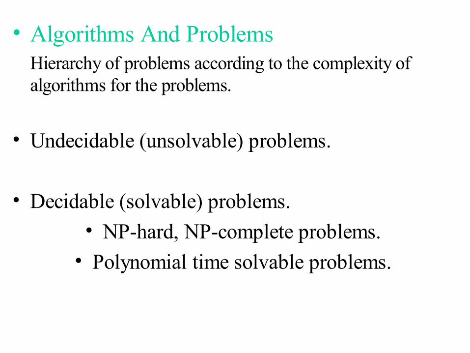
• Algorithms And Problems

Hierarchy of problems according to the complexity of algorithms for the problems.

• Undecidable (unsolvable) problems.

• Decidable (solvable) problems.• NP-hard, NP-complete problems.

• Polynomial time solvable problems.

Figure 1: An simple illustration of complexity of problems

• Undecidable (unsolvable) problems: (No algorithm exists)

The Halting problem: Does there exist a program (algorithm/Turing machine) Q to determine, for arbitrary given program P and input data D, whether

or not P will halt on D?

Post's correspondence problem

A correspondence system is a finite set P of ordered pairs of nonempty strings. A match of P is any string w ∈ ∑∗ such that for some n>0 and some pairs (u1, v1), (u2, v2),...,(un, vn) ∈P, w = u1u2...un = v1v2...vn.

For example If P = (a, ab), (b, ca), (ca, a), (abc, c), then w=abcaaabc is a match of P, since if the following sequence of five pairs is chosen, the concatenation of the first components and the concatenation of the second components are both equal to w= abcaaabc : (a, ab), (b, ca), (ca, a), (a, ab), (abc, c).

The post's correspondence problem is to determine given a correspondence system whether that system has a match.

Hilbert’s tenth problem

• To devise an `algorithm’ that test whether or not a polynomial has an integral root.

• A polynomial is a sum of terms. For example, 6x3yz2 + 3xy2 - x3 – 10 An integral root is a set of integer values

setting to the polynomial so that it will be zero.

For example, the above polynomial has an

Integral root: x=5, y=3, z=0 (135-125-10=0).• Let D denote a set of polynomials so that

D = p | p is a polynomial with an integral

root

Hilbert’s tenth problem becomes

Is D decidable?

The answer is that it is not decidable.

A brief idea of proof• Let D’ be a set of special polynomials that p has

one variable. I.e., D’=p | p is polynomial over x with an integral root. For example, 4x3 - 2x2 + x – 7• Let M’ be a Turing Machine that input: a polynomial p over the variable x. Program: Evaluate p with x set successively to the

values 0, 1, -1, 2, -2, 3, -3, … If at any point the polynomial evaluated to zero, accept.

• M’ recognizes D’.• For general polynomial, we can devise a Turing

machine M to recognize D similarly.

To set successively the values of all combinations to the variables, if the polynomial evaluated to zero, accept.

For example, x 0 0 1 0 -1 0 2 0 …

y 0 1 0 -1 0 2 0 -2 …

Can you set the value pattern as

x 0 0 0 0 0 … 1 1 1 1 1 …

y 0 1 -1 2 -2 … 0 1 -1 2 -2 … ?

• M’ can be modified as decidable with D’.

The bound of the value of the single variable can be calculated. For example,

4x3 - 2x2 + x – 7 has a bound of |x| < 7.

Since the bound is finite, if the value has

exceeded the bound and the polynomial is

not evaluated to zero, then stop. Thus,

M’ can decide D’.

• The general bound for D’ is |k Cmax/C1|.

• Matijasevic proved no such a bound for D.

An intuitive proof of Halting problem

• Let us assume there exits an algorithm Q

with such a property, i.e., Q(P(D)) will be

run forever if arbitrary algorithm P with

input data D, P(D) run forever.

halt if P(D) halts.

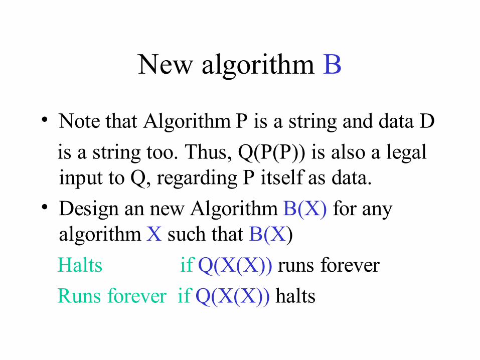
New algorithm B

• Note that Algorithm P is a string and data D

is a string too. Thus, Q(P(P)) is also a legal input to Q, regarding P itself as data.

• Design an new Algorithm B(X) for any algorithm X such that B(X)

Halts if Q(X(X)) runs forever

Runs forever if Q(X(X)) halts

The construction of B

• Note that B can be constructed because Q can be constructed. For example, we may build B on Q as follows: When Q detects P(D) stops and Q shall stop, but we modify Q (called B) and let B run forever; while Q detects P(D) runs forever and Q shall run forever, but we modify Q (called B) and let B stop.

ContradictionLet B run with input data B, then B(B) will

either halt or will run forever, and this can be detected by Q(B(B)).

• If B(B) stops, hence Q(B(B)) stops and forces B(B) runs forever by the construction of B.

--- B(B) enters both stop and run forever.

continuous• If B(B) runs forever, then Q(B,B) runs

forever and forces B(B) stops.

--- B(B) enters both stop and run forever.

• --- All statements are logically followed

the assumption --- assumption is wrong --- there cannot exist such a program Q.

The diagonalization method• This method is due Georg Cantor in 1873.• Definitions: one-to-one function f : A to B

if it never maps two different elements to the same place. f is onto if it hits every element of B. f is correspondence if it is both one-to-one and onto.

• Correspondence is to pair the elements in A and B.

• The correspondence can be used to compare the size of two sets. Cantor extended this idea to infinite set.

• Definition: A set A is countable if either it is finite or it has the same size as natural numbers N.

For example, N = 1,2,3,…, E=2,4,6,…, O=1,3,5,… are same size and hence countable.

Q be set of rational numbers:

Q=m/n | m, n in N

1/1 1/2 1/3 1/4 1/5 ……

2/1 2/2 2/3 2/4 2/5 ……

3/1 3/2 3/3 3/4 3/5 ……

4/1 4/2 4/3 4/4 4/5 …..

5/1 5/2 5/3 5/4 5/5 ……

.

. Q is countable.

• Real numbers R is uncountable.

Let f make correspondence between N and R.

n f(n)

1 3.14159265…

2 55.55555555…

3 1.41427689…

4 0.50000000…

. ……..

• Construct a real number x by giving its decimal

representation such that x is not belong to any f(n).

• To do that, we let the first digit of the first real be different from the first digi of x, say x=.2; then let the second digit of the second real be different from the second digit of x, say x=.34; so on so forth.

• The new real number x=.34…. is different from any real in the table by at least one digit difference. Therefore, x does not correspondence to any natural number and is uncountable. (can we choose 0 and 9 as digits in x?)

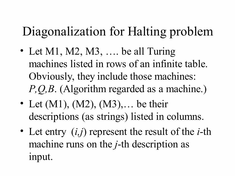
Diagonalization for Halting problem

• Let M1, M2, M3, …. be all Turing machines listed in rows of an infinite table. Obviously, they include those machines: P,Q,B. (Algorithm regarded as a machine.)

• Let (M1), (M2), (M3),… be their descriptions (as strings) listed in columns.

• Let entry (i,j) represent the result of the i-th machine runs on the j-th description as input.

(M1) (M2) (M3) … M1 accept rej/nstop accept … M2 accept accept rej/nstop … M3 rej/nstop accept rej/nstop … . ………………. . .

• When a machine M runs on a description as input, it either accept or reject or nonstop.

• When a machine Q runs on a description (machine M runs on input D), it either accept or reject.

(M1) (M2) (M3) … M1 accept reject accept … M2 accept accept reject … M3 reject accept reject … . ………………. .

• When a machine B runs on a description (machine B runs on input D), it both accept and reject.

(M1) (M2) (M3) … (B) …

M1 accept reject accept … M2 accept accept reject … M3 reject accept reject … . ………………. B reject reject accept ? …

.

Polynomial time decidable problems: (Algorithms exist and relatively efficient)

• Sorting a set of elements. Find the maximum, minimum, and median of a set of elements, Matrix multiplication. Matrix-chain multiplication, Single source shortest path. Convex hull of a set of points. Voronoi diagrams. Delaunay triangulations.

• NP-hard, NP-complete problems: (Algorithms exist, but not efficient)

• Boolean Satisfiability problem, vertex cover problem. Hamiltonian-cycle problem.

A hamiltonian cycle of an undirected graph G=(V,E) is a simple cycle that contains each vertex in V. Does a graph G have a hamiltonian cycle? Traveling salespersons problem (Ω(m!), where m is the number of vertices in V.)

The measurement of the efficiency of algorithms

– (1) The worst-case time (and space). Insertion

sort O(n2) in worst-case time. – (2) The average-case time.

Quick sort O(n log n) time in average-case, O(n2) in worst-case time.

Other analysis methods:

• The amortized analysis • The randomized analysis

In an amortized analysis, the time complexity is obtained by taking the average over all the operations performed. Even though a single operation in the sequence of operations may be very expensive, but the average cost of all operations in the sequence may be low.

Example: Incrementing a binary counter. We shall count the number of flips in the counter when we keep adding a one from its lowest bit.

• 0 0 0 0 0 0 0 0 • 0 0 0 0 0 0 0 1 • 0 0 0 0 0 0 1 0 • 0 0 0 0 0 0 1 1 • 0 0 0 0 0 1 0 0 • 0 0 0 0 0 1 0 1 • 0 0 0 0 0 1 1 0 • 0 0 0 0 0 1 1 1 • 0 0 0 0 1 0 0 0• 1 1 1 1 1 1 1 1

• Increment(A) i ← 0 While i < length[A] and A[i]=1 Do A[i] ← 0

i ← i+1 If i < length[A] Then

A[i] ← 1

• In the conventional worst-case analysis, consider all k bits in the counter are `1's. any further increasing a `1' will cause k flips. Therefore, n incremental will cause O(kn) flips.

• Note that A[1] flip every time, A[2] flip every other time, A[3] flip every foutrth time,..., A[i] flip every 2ith time.

• Thus, we have that ∑ log n

i=0 n/2i< n∑∞

i=01/2i = 2n.

The average cost of each incremental is O(1), not O(k).

• Optimal Algorithms • Upper bound of a problem

– (1) the number of basic operations sufficient to solving a problem

– (2) the minimum time complexity among all known algorithms for solving a problem

– (3) upper bound can be established by illustrating an algorithm.

• lower bound of a problem

(1) the number of basic operations necessary to solving a problem

(2) the maximum time complexity necessary by any algorithm for solving a problem

(3) lower bound is much more difficult to establish.

• An algorithm is optimal if its time complexity (i.e., its upper bound) matches with the lower bound of the problem. For example, the problem of sort n elements by comparisons. Lower bound = log2 n! as there are n! different outcomes (permutations) and any decision tree which has n! leaves must be of height >= log2 n! .Clearly, Merge-sort algorithm is optimal and insertion sort is not.

• While you may already learn some methods of lower bound establishment such as decision tree and adversary (oracle), we shall also introduce a very useful method: Establish upper and lower bounds by transformable problems.

Decision tree.

Adversary.

Transformation.

Figure 2Transfer of upper and lower bounds between transformable problems.

• Suppose we have two problems, problem α and problem β, which are related so that problem α can be solved as follows: – 1. The input to problem α is converted into a

suitable input to problem β. – 2. Problem β is solved. – 3. The output of problem β is transformed into a

correct solution to problem α– We then say that problem α has been

transformed to problem β. If the above transformation of step 1 and step 3 together can be done in O(τ(N)) time, where N is the size of problem α, then we say that α is τ(N)- transformable to β

– Proposition 1 (Lower bound via transformability). If problem α is known to require at least T(N) time and α is τ(N)-transformable to problem , then β requires at least T(N) - O(τ(N)) time.

– Proposition 2 (upper bound via transformability). If problem β can be solved in T(N) time and problem α is τ(N)-transformable to problem , then α can be solved in at most T(N) + O(τ(N)) time.

βα τ )(N∝

βα τ )( N∝

• For example. Element Uniqueness: Given N real numbers, decide if any two are unique. (Denote this problem as α.)

This problem is known to have a lower bound. In the algebraic decision tree model any algorithm that determines whether the member of a set of N real numbers are distinct requires Ω(N log N) tests.

Now, we have another problem, Closest Pair: Given N points in the Euclidean plane, find the closest pair of points (the shortest Euclidean distance). Denote this as β.

• We want to find the lower bound of this problem. (Can we use decision tree method or adversary method to this problem?)

• We transfer Element Uniqueness problem to Closest Pair problem. Given a set of real numbers (x1, x2, ..., xN) (INPUT to α), treat them as points in the y=0 line in the xy- coordinate system (convert them into a suitable input of β). Apply any algorithm to solve β. The solution is the closest pair. If the distance between this pair is nonzero, then the points are distinct, otherwise it is not. (Convert the solution of β to the solution of α.) τN= O(N). By Proposition 1, β takes at least Ω(N log N) - O(N) time, which is the lower bound.

• Using the same method, we can prove that the lower bound of sorting by comparison operations is Ω(n log n), by transferring the Element Uniqueness to Sorting. The lower bounds of a chain of problems can be proved in this manner.

Reduction for intractability

• The above transformation method can be used for proving a problem is intractable

or tractable if the cost of transformation is bounded by a polynomial.

For example,CLIQUE: Instance: A graph G=(V,E) and a positive

integer J <= |V|.

Question: Does G contain a clique of size J

or more? That is, a subset V’ in V such that

|V’| >= J and every two vertices in V’ are joined by an edge in E.

• VERTEX COVER (VC):

Instance: A graph G=(V,E) and a positive integer

k <= |V|.

Question: Is there a vertex cover of size k or less for G? That is, a subset V’in V such that |V’|<=k and for each edge in E at least one of the endpoints is in V.

Let A be VC and B be clique

• For every instance of A, we can convert it to an instance of B in polynomial time.

Let G=(V,E) and k <= |V| be an instance of VC. The corresponding instance of Clique is Gc and the integer j=|V|-k.

• For covert the output of B to an output of A in polynomial time (constant time yes/no).

=> If A is intractable, then B is intractable.

• For every instance of B, we can convert it to an instance of A in polynomial time.

Let G=(V,E) and j <= |V| be an instance of Clique. The corresponding instance of VC is Gc and the integer k=|V|-j.

=> If B is tractable, then A is tractable.

Reduction for decidability

• Mapping reducibility: If there is a computable function f: for every w in A, there is an f(w) in B.

• f is called the reduction of A to B.• If A <m B, and B is decidable, then A is

decidable.• If A <m B, and A is undecidable, then B is

undecidable.

Post correspondence problem

• Some instance has no match obviously.

(abc, ab) (ca, a) (acc, ba) since the first element in an order pair is always larger than the second.

• Let us define PCP more precisely:

PCP=[P] | P is an instance of the Post

correspondence problem with a match

Where P=t1/b1, t2/b2, … tk/bk, and a match

is a sequence i1, i2 , …, is such that

ti1 ti2… tis = bi1 bi2… bis .

• Proof idea: To show that for any TM M and input w, we can construct an instance P such that a match is an accepting computation history for M on w. Thus, if we can determine whether the instance P has a match, we can determine whether M accepts w (halting problem).

• Let us call [ti/bi ] a domino.

In the construction of P, we choose the dominos so that a match forces a simulation of M to accept w.

• Let us consider a simpler case that M on w does not move its head off the left-hand end of the type and the PCP requires a match always starts with [t1/b1. ] Call it MPCP.

MPCP=[P] | P is an instance of the Post

correspondence problem with a match

starting at [t1/b1].

Proof. Let TM R decide the PCP and construct TM S to decide ATM.

M =(Q,Σ, Γ, δ, qo, qaccept, qreject,),

where Q is the set of states, Σ is the input alphabet, Γ is the tape alphabet, δ is the transition function of M.

S constructs an instance of PCP P that has a match if and only if M accepts w.

• The construction of P’ of MCPC consists of 7 parts.

1. Let

[#

# qo w1 ww… wn]

be the first domino in P’, where C1 =qo w

= qo w1 ww… wn is the first configuration of M and # is the separator.

The current P’ will force the extension of the top string in order to form a match.

To do so, we shall provide additional dominos to allow this, but at the same time these dominos causes a single step simulation of M, as shown in the bottom part of the domino.

Parts 2, 3, and 4 are as follows:

2. For every a, b in Γ and every q, r in Q, where q is not q reject if δ( q, a) = (r ,b ,R),

put [qa/br] into P’. (head moves right)

3. For every a, b, c in Γ and every q, r in Q, where q is not q reject if δ( q, a) = (r ,b ,L),

put [cqa /rcb] into P’. (head moves left)

4. For every a in Γ , put [a/a] into P’. (head is not on symbol a)

What do the above construction parts mean?

Consider the following example: Let Γ =0, 1, 2, e, where e is empty, w= 0 1 0 0 , and the start state of M is qo.

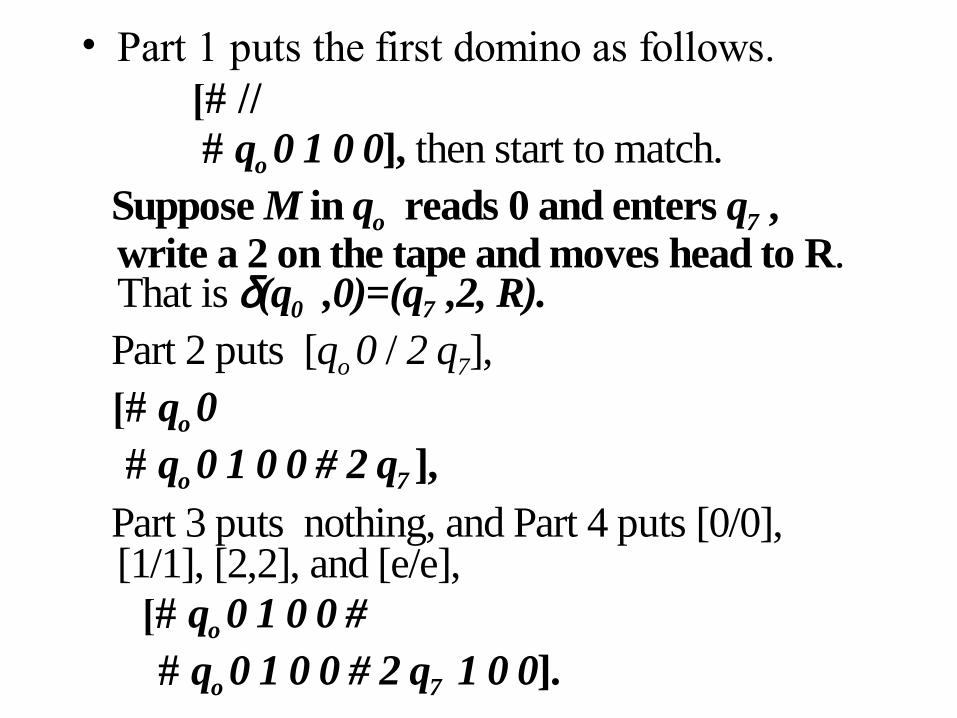
• Part 1 puts the first domino as follows. [# // # qo 0 1 0 0], then start to match. Suppose M in qo reads 0 and enters q7 ,

write a 2 on the tape and moves head to R. That is δ(q0 ,0)=(q7 ,2, R).

Part 2 puts [qo 0 / 2 q7], [# qo 0 # qo 0 1 0 0 # 2 q7 ], Part 3 puts nothing, and Part 4 puts [0/0],

[1/1], [2,2], and [e/e], [# qo 0 1 0 0 # # qo 0 1 0 0 # 2 q7 1 0 0].

Part 5 for copy the # symbol to separate different configuration of M. I.e., put [#/#] and [#/e#] into P’. The second domino allow us to add an empty symbol e to represent infinite number of blanks to the right.

Thus, the current P’ has two configurations

separated by #.

[# qo 0 1 0 0 # //

# qo 0 1 0 0 # 2 q7 1 0 0 #].

Now, suppose M in q7 reads 1 and enters q5 , write a 0 on the tape and moves head to R .

That is, δ(q7 ,1)=(q5 ,0, R).

We have that

[# qo 0 100 # 2 q7 1 0 0 # //

# qo 0100 # 2 q7 1 0 0 # 2 0 q5 0 0 #].

Then, suppose M in q5 reads 0 and enters q9 , write a 2 on the tape and moves head to L .

That is, δ(q5 ,0)=(q9 ,2, L).

We have dominos: [0q50 / q9 02], [1q50 / q9 12],

[2q50 / q9 22], and [eq50 / q9 e2]. Only the first domino fits.

[# qo 0100 # 2 q7 100 # 20 q5 00 #

# qo 0100 # 2 q7 100 # 20 q5 00 # 2 q9 020 # ].

This process of match and simulation M on w continue until q accept has been reached.

We need to make a catch up for the top part of the current P’. To do so, we have part 6.

6. For every a in Γ , put

[a qaccept / qaccept ] and [qaccept a / qaccept ] into P’.

This is to add pseudo-steps to M after halted

as the head eats the adjacent symbols until no

symbol left.

Suppose that M in q9 reads 0 and enters

qaccept.

[# qo 0100 # 2 q7 100 # 20 q5 00 #

# qo 0100 # 2 q7 100 # 20 q5 00 # 2 q9 020 # ].

[…#20q500#2q9020 #

…#20q500#2q9020 #2qaccept20#]

[…#20q500#2q9020 #2qaccept20#

…#20q500#2q9020 #2qaccept20#2qaccept0#]

[…#2q9020 #2qaccept20#2qaccept0#

…#2q9020 #2qaccept20#2qaccept0#2qaccept#]

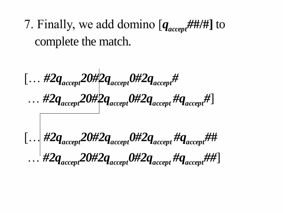
7. Finally, we add domino [qaccept##/#] to complete the match.

[… #2qaccept20#2qaccept0#2qaccept#

… #2qaccept20#2qaccept0#2qaccept #qaccept#]

[… #2qaccept20#2qaccept0#2qaccept #qaccept##

… #2qaccept20#2qaccept0#2qaccept #qaccept##]

To remove the restriction on P’. I.e., start at the first domino, we add some symbols to

every element of P’.

If P’ = [t1/b1],[ t2/b2], …, [tk/bk] is a match,

then we let

P=[*t1/*b1*],[ *t2/b2*], …, [*tk/bk*], [*o/o].

Clearly, PCP must start at the first domino.

[*o/o] for allowing the top of P to add #.

Algorithm design methods • Divide-and-Conquer Generic Algorithm. Divide: partition the (input of) original

problem into two smaller problems. Conquer: Solve the smaller problems, recursively.

Combine: The solutions of the two smaller problems are combined into the solution of the original problem.

The efficiency of this paradigm relies on the efficiency of step Combine.

• For example: Merge-sort has a linear-time merge procedure to merge two sorted lists into one sorted list.

1 9 5 3 6 2 7 4

1 9 3 5 2 6 4 7

1 3 5 9 2 4 6 7

1 2 3 4 5 6 7 9

• Find the median of a set of n elements in linear time.

Figure 3: For the Algorithm Select.

• Algorithm Select. 1.divide the n elements of the input array into n/5 group of 5 elements each and at most one group made up of the remaining nmod 5 elements.

2. Find the median of each of the n/5 groups by first insertion sorting the elements of each group and then picking the median from the sorted list of group elements.

3. Use select recursively to find the median x of the n/5 medians found in step 2. (Choose the lower one if there are even number of medians.)

• 4. Partition the input array around the median-of-medians x using the modified version of partition. Let k be one more than the number of elements on the low side of the partion, so that x is the kth smallest element and there are n-k elements on the high side of the partition.

• 5. If k=n/2, then return x, otherwise, use select recursively to find the median on the low side if n/2<k, or on the high side if n/2>k.

• The number of elements greater than x is at least 3( 1/2 n/5 -2 ) ≥ (3n)/10-6.

The number of elements less than x is at most (7n)/10+6. (Refer to the figure.)

In the worst case, this algorithm is recursively called on at most (7n)/10+6 element in Step 5.

Note that the recursive call in Step 3 yields T(n/5). Steps 1, 2, and 4 take O(n) time. Thus, we have the recurrence.

• Recurrence. T(n)≤T(n/5)+T((7n)/10+6) + O(n) if n≥ 140;

Θ(n) otherwise. • To solve this recurrence. T(n) ≤ cn/5 +

c((7n)/10+6) + an ≤ c n/5 +c + (7cn)/10+6c+an = (9cn)/10+7c + an =cn + (-(cn)/10 +7c + an).

• If (-(cn)/10 +7c +an) ≤ 0, then T(n) ≤ cn ∈ O(n).

• It follows if c ≥ 10a(n/(n-70)) when n > 140, choose c ≥ 20a will do.

• Dynamic Programming Matrix-Chain multiplication problem. Given a sequence (chain) of matrices , multiple

them to obtain the product with the minimum number of multiplication operations.

For example, given a chain of four matrices A1A2A3A4, there are five possible associations. If we give the size of these matrices as follows, then there will have different number of multiplication operations.

2 × 5, 5 × 3, 3 × 4, 4 × 6 be the size of corresponding matrix.

(A1(A2(A3A4)))

(2 × 5 × 6 + 5 × 3 × 6 + 3 × 4 × 6 = 222)(A1((A2A3)A4))

(5 × 3 × 4 + 5 × 4 × 6 + 2 × 5 × 6 = 240)((A1A2)(A3A4))

(2 × 5 × 3 + 3 × 4 × 6 + 2 × 3 × 6 = 138) ((A1(A2A3))A4)

(5 × 3 × 4 + 2 × 5 × 4 + 2 × 4 × 6 = 148) (((A1A2)A3)A4)

(2 × 5 × 3 + 2 × 3 × 4 + 2 × 4 × 6 = 102) An optimal solution can be found

by exhausting all the possible associations, which takes O(4n/n2) time (Catalan number).

Does Divide-and-conquer work for this problem? No.

(The solution after the combination of the solutions of smaller problems may not be the optimal one (the original one) if our partition is ` half-and-half' as the shown in the third row.)

• The essence of dynamic programming method is that – (1) Dynamic programming method calculates the

solution to all subproblems; – (2) the computation proceeds from the small

subproblems to the large subproblems; – (3) Storing the solutions in an table so that they

can be reused without recomputing the subproblems again.

– Dynamic programming relies on two properties of problems: the principle of optimality and overlapping subproblems.

• Optimality: if the partition between kth and k+1th matrices (A1 .... Ak)(Ak+1Ak+2...An) belongs to optimal associations (the last one), then any other optimal associations (say, the two second last associations) must lie within each subchain, (A1 .... Ak) and (Ak+1Ak+2...An) respectively. In other words, the second last association is also an optimal association for the subproblem. They can be determined in their corresponding subchains, respectively. Overlapping subproblems: Let Ai...Aj be a subchain of matrices A1...An. (see the figure)

Figure 4: Illustrating the overlapping subproblems.

3 partitions

Recurrence

• Let mi,j be the minimum number of multiplications for finding the product of this subchain. We have the following recursive formula to find the solution. mi,i=0, mi,i+1=pi-1pipi+1, where Ai has size of pi-1 × pi and Ai+1 has size of pi × pi+1.

mi,i+s = mini ≤ k < i+s(mi,k + mk+1,i+s + pi-1pkpi+s) Where 1 ≤ i ≤ n-s.

• The problem can be solved in O(n3) time.

• Greedy Method

Greedy method enjoys its simplicity. A greedy method generally only looks for local information to make its decision. For example, Prim's algorithm for finding the minimum spanning tree of a connected, undirected graph.

The algorithm starts at the source vertex; choose one of its incident edges satisfying the following criteria:

(a) It has the smallest weight among all the edges incident to this vertex; and

(b) add this edge to the partially built MST such that the partial MST does not form a cycle;

The algorithm grows the MST by adding such edges until either a complete MST is found or there are no edges left to be added.

Figure 5: Illustrating the Prim's algorithm.

• Often, greedy algorithm may not yeild an optimal solution. For example, the 0-1 Knapsack problem.

If we take the greatest value per pound for the criterion of greedy, it may not yield optimal solution.

• Fractional Knapsack problem using greedy

method can yield an optimal solution.

Figure 4: The greedy strategy does not work for the 0-1 knapsack problem.