create, design, engineer! - 北京天源博通科技有限公 … winding copper losses motor drive...

GOT-It - Optimization with Flux October 2012

1

Create, Design, Engineer!

GOT-ItOptimizing PM Machines

xxx

www.magsoft-flux.comwww.cedrat.com

Philippe [email protected]

2

Introduction: The Optimization

Find the best value of input parameters that maximizes or minimizes an objective function taking into account constraints

Use optimization algorithms that propose search strategies to find the optimum, based on evaluations of the objective function.

F

xX_opt

F

xX_opt

F(x)

Optimization algorithm

Objective function

(X_opt)


2

3

General optimization strategies…

Deterministic algorithms (SQP, Conjugate gradients,…)• Fast

• Based on local function variations

• Efficient to find local optimum

• Need gradients of the functions

Stochastic algorithms (Genetic algorithms, Niching,…)• Time-consuming

• Based on wide number of trials

• Efficient to find the global optimum

• Do not need gradients of the functions

F

x

4

Based on numerical models…

The time to evaluate the objective functions must be minimal:

• Each Finite Element evaluation is costly,

• They must be performed many times.

A good approach is based on Design Of Experiment.

Two strategies:• Reduce the number of input parameters: Screening,

• Use indirect optimization: Response Surface Methodology.F

x

F’(x)= a0 +a1.x1+a2.x2+a12.x1²+a22.x2²+a3.x1.x2 Design of Experiment tables


3

5

Strategy to reduce the size

Screening: detect the most influent parameters:• Can sort a large number of parameters,

• Reduce needed set of calculations.

6

Strategy to reduce computation time

Indirect Optimization: Response surface method

F

Design of Experiment tables

Response surface Method

xtable

x Sf(x)

f(xtable) Few costly calls

Objective function (FE calculation)

Numerous cheap calls

Optimization algorithm

Response surface (Surrogate function)

Build surrogate functionx

Sequential Surrogate optimizer (SSO)Response surface Indirect

optimizationResults RS

Results Flux


4

7

An Industrial and Multipurpose Tool

A wide range of applications: Minimize losses in a machine,

Minimize torque ripples,

Minimize time-response of an actuator,

Reduce electric field along a path,

Maximize efficiency ofelectromechanical conversion.

8

GOT-It Features…

Continuous and/or discrete parameters,

Single or multi-objective functions,

Constrained or unconstrained optimization,

Analytical functions or functions derived from numerical models,

Design Of Experiments (DOE),

Response surfaces (polynomial, RBF, kriging, Space Mapping).

Direct or indirect (SRM) optimization techniques.

Deterministic (CG, BFGS) or stochastic (GA, Niching, PSO) algorithms,

Post-processing (curves, surfaces, Pareto frontiers, sensitivity analysis, automatic report).


5

9

Basic Operation

Define the optimization problem • Objective function

(mono or multi-objective)

• Constraints

• Variations of input parameters

Choose an optimization algorithm and run it• Deterministic or stochastic

• Can be chosen automatically by GOT-It

Post-process the results • Draw curves

• Create automatic report (html format)

F

x

Feasible

G(X) <0

G(X) >0

Infeasible

F

xx_opt

10

GOT-It interface

Data tree Information

Menus bar

Console

Title bar


6

11

GOT-It contexts

Context Allows mainly…

ParametricParametric enhanced

Handling parametric studies

Screening Finding the most influent parameters

Model reduction Building response surfaces

OptimizationOptimization enhanced

Defining optimization problems, choosing optimization algorithms, launching optimizations and analyzing the optimum solutions

Expert using expert functionalities

The selected context determines the level of use

12

GOT-It entitiesThe selected context also determines the entities used

ParameterFunctionFunction vectorSurrogate factorySurrogateOptimization problemOptimization algorithmOptimizationOptimization problem factoryStochastic operator

Connector and Analysis tool are available in all contexts

ParametricParametric enhanced

ScreeningModel reduction

OptimizationOptimization enhanced

Expert


7

13

GOT-It analysis tools…Evaluator : F(x1,x2,…,xn) evaluation for reference values

of xn

Curve plotting : variation curve of F(x)

Surface plotting : variation surface of F(x1,x2)

Isoval plotting : parametric isovalues

Screening analyzer : sensitivity analysis of F(x1,x2,…,xn)

Variation plotting : Function variations around the optimum

Stochastic evaluator : robustness analysis

Pareto frontier : Pareto frontier in multi-objective optimizations

14

GOT-It – Flux coupling set up1) Export coupling component from

Flux project2) Create Flux communicator

in GOT-It project

Select (.F2G) file exported from Flux

Input parameters:Geometric parametersParameters I/O (scenario)

Parameters I/O (formula)Sensors

Output functions:

FluxFileForGOT-It.F2G.FLU LinkComponent.F2G


8

15

Coupling technology

GOT-It drives optimization based on CEDRAT tools simulations

Available in Flux v10.4.1 and subsequent versions 2D, 3D and Skew applications (according to the Flux license)

Need to launch Flux in advanced mode

16

Post processing command files

Specified in the coupling component for GOT-It

Used at each Flux evaluation

To get the min, max, mean value of a 2D curve

To get the time response

To compute losses, performances, cogging torque,…


9

17

See how it works!

18

Example 1: Minimize Core Losses and Cogging Torque

Industrial Application Motor pump

Water cooled

General Characteritics Constant speed operation at 2000 rpm

0.7 hp

4 poles

24 slots

3 Phase Y connected winding

Drive Information Sine

48 Volts

50 Amps max


10

19

Brushless PM Motor Dimensions/Materials

Motor Key Dimensions

Motor Materials Stator laminations: M19 24 Gauge equivalent

Rotor hub: 430F

Magnet: Ferrite grade

20

Motor Performances

Motor Magnetic Flux and Saturation


11

21

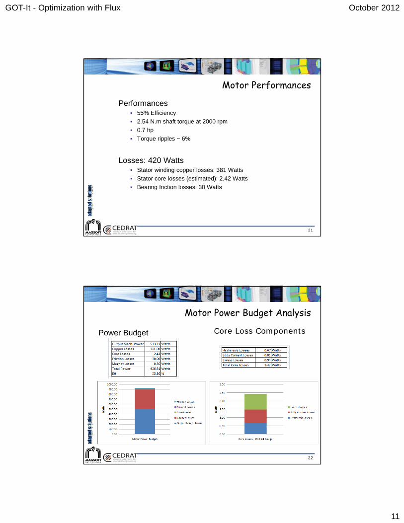
Motor Performances

Performances 55% Efficiency

2.54 N.m shaft torque at 2000 rpm

0.7 hp

Torque ripples ~ 6%

Losses: 420 Watts Stator winding copper losses: 381 Watts

Stator core losses (estimated): 2.42 Watts

Bearing friction losses: 30 Watts

22

Motor Power Budget Analysis

Power Budget Core Loss Components


12

23

Losses Minimization and Torque Ripples Reduction

Objective Increase motor efficiency by reducing the motor losses

Reduce torque ripples

Strategy: 2 approaches 2 sequential optimization problems with constraints

• Losses minimization

• Torque ripples minimization

Single step multi-constraints losses and torque ripplesminimization

• Objective: minimum losses

• Constraint: torque ripples below 4.5%

24


The Parameters

Geometric Magnet arc A_BetaM

Magnet edge A_Edge

Magnet thickness A_LM

Stator slot opening A_SO

Stator slot angle A_SOAng

Stator tip thickness A_TGD

Physics Motor drive rms current Airms

Magnet remanent flux density Abr


13

25


26

Method 1 - Screening and 2 StepsOptimization

Screening and Identification

Separation of losses minimization and torque ripples reduction Significant stator winding copper losses

Motor magnetics not saturated

Losses main contributor and key parameter Stator winding copper losses

Motor drive current

Constraint on minimum torque requirement => stronger magnet

Torque ripples reduction Shaping of stator tooth geometry

Shaping of magnet

Constraint on minimum torque requirement


14

27

Screening and 2 Steps OptimizationStep 1 Losses Minimization

Optimization Algorithm Sequential quadratic programming

Results Winding losses are reduced from 382 Watts to 96 Watts

Current is reduced from 30 Amps to 15.4 Amps

Magnet Br is increased from 0.41 T to 0.8 T

3 SQP iterations

28

Screening and 2 Steps OptimizationStep 1 Losses Minimization

Results: motor losses objective function and torque constrainst


15

29

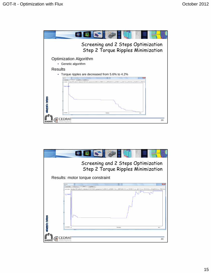
Screening and 2 Steps OptimizationStep 2 Torque Ripples Minimization

Optimization Algorithm Genetic algorithm

Results Torque ripples are decreased from 5.6% to 4.2%

30

Screening and 2 Steps OptimizationStep 2 Torque Ripples Minimization

Results: motor torque constraint


16

31

Method 2 - Losses Minimization withTorque Constraints

Objective Function Motor losses

Constraint Minimum torque requirement

Torque ripples less than 4.5%

Results Achieved motor losses: 217.31 Watts

Resulting torque ripples 3%

32

Losses Minimization with Torque Constraints

Results


17

33

Results Summary

Name Initial Optimum 1 Optimum 2 Motor Phase Current (Amps

rms) A_IRMS 30.00 15.40 21

Magnet Br A_Br 0.41 0.8 0.69 Slot Opening in mm A_SO 0.90 0.82 1.75

Stator Tooth Angle in deg. A_SOAng 20.00 10.00 39.9 Tooth Tip Thickness in mm A_TGD 1.00 0.80 2.00 Magnet Thickness in mm A_LM 5.50 5.56 7.73 Magnet Arc Angle in deg. A_BetaM 150.00 152.80 152.2

Magnet Edge Height in mm A_Edge 5.50 5.30 4.86 Motor Losses in Watts Lossesmotor 413.42 130.67 217.31 Average Torque in N.m T_Ave 2.51 2.50 2.5

Torque Ripples in % T_Ripples 5.56 4.21 3.01

34

Optimization Results


18

35

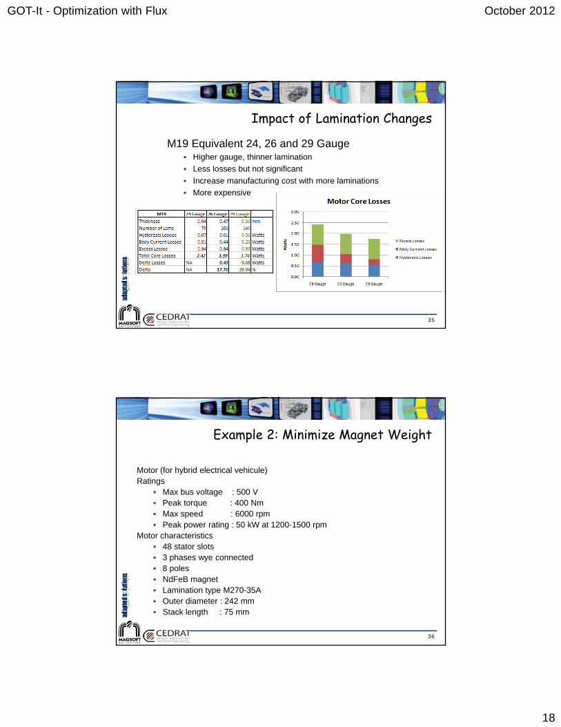
Impact of Lamination Changes

M19 Equivalent 24, 26 and 29 Gauge Higher gauge, thinner lamination

Less losses but not significant

Increase manufacturing cost with more laminations

More expensive

36

Example 2: Minimize Magnet Weight

Motor (for hybrid electrical vehicule)Ratings

Max bus voltage : 500 V Peak torque : 400 Nm Max speed : 6000 rpm Peak power rating : 50 kW at 1200-1500 rpm

Motor characteristics 48 stator slots 3 phases wye connected 8 poles NdFeB magnet Lamination type M270-35A Outer diameter : 242 mm Stack length : 75 mm


19

37

The machine: the real design

38

Our starting design: larger magnets, deeper pole piece


20

39

Starting Design – Flux Lines

40

Starting Design – Flux Density


21

41

Screening: 6 Geometric Parameters

42

Screening: 6+2 Parameters

Physics Parameters


22

43

Box 64 Screening 8 Parameters

44

Screening Results Box 64

Given the range of exploration set for each parameter:

As expected LM and MAGWID are the key parameters – we are trying to minimize weight,

Br has little impact – within the range of exploration

BETAM seems to have limited impact

The screening is run with only 5 parameters

Solutions evaluated during screening are the basis for the final optimisation


23

45

First run: 5 Parameters

46

Taguchi 16 Screening 5 par.


24

47

Improved Design – 5 Parameters

48

Magnet Xsection Area

Init – 450 mm^2 Improved – 308 mm^2


25

49

Improved Design

50

Initial Design

Improved Design

Commercial Design

Units

BetaM 150 140 140 eDegIPMHQ 15 13.3 10 mmLM 9 5.6 5 mmMagWid 50 55 54 mmLm x MagWid

450 308 270 mm^2

Lweb 2.75 1.3 2.75 mmWeb 10 10 10 mmGamma 45 52 45 eDegBr 1.15 1.15 1.2 TeslaAve_Torque 413 401 390 N.mMax_Torque 467 453 435 N.mMin_Torque 340 337 344 N.m


26

51

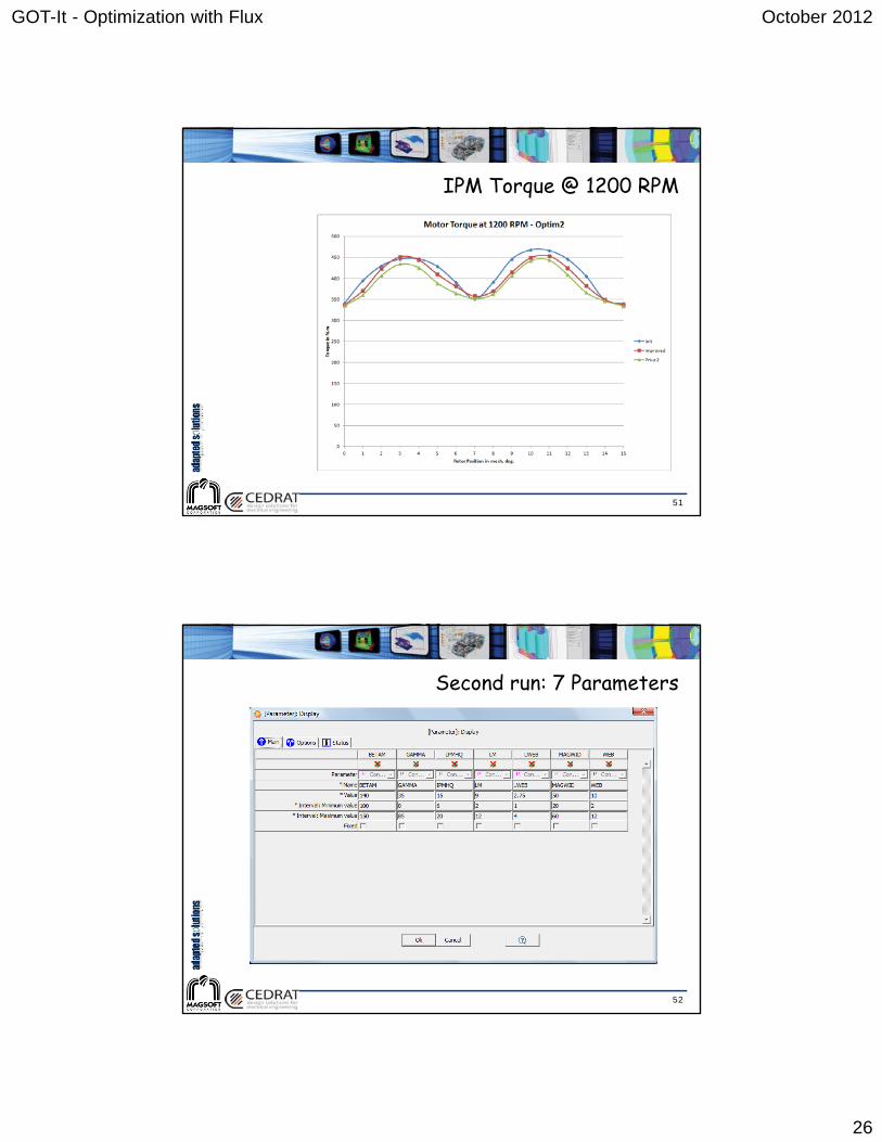
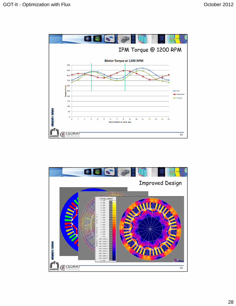
IPM Torque @ 1200 RPM

52

Second run: 7 Parameters


27

53

Magnet X-section Area

Init – 450 mm^2 Improved – 264 mm^2

54

Results SummaryInitial Design

Improved Des.

CommercialDesign

Units

BetaM 140 105 140 eDegIPMHQ 15 11.5 10 mmLM 9 6 5 mmMagWid 50 44 54 mmLm x MagWid

450 264 270 mm^2

Lweb 2.75 2.65 2.75 mmWeb 10 10.6 10 mmGamma 35 52 45 eDegBr 1.15 1.15 1.2 TeslaAve_Torque 413 402 390 N.mMax_Torque 467 447 435 N.mMin_Torque 340 361 344 N.m


28

55

IPM Torque @ 1200 RPM

56

Improved Design


29

57

Objective Function Convergence

58

PU Magnet Volume


30

59

Evaluation of MagWid & LM

60

Torque Constraints


31

61

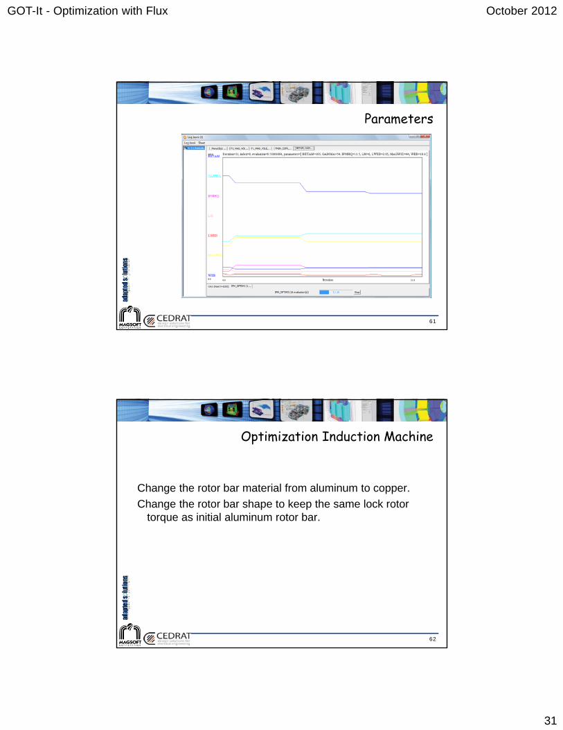
Parameters

62

Optimization Induction Machine

Change the rotor bar material from aluminum to copper.

Change the rotor bar shape to keep the same lock rotor torque as initial aluminum rotor bar.


32

63

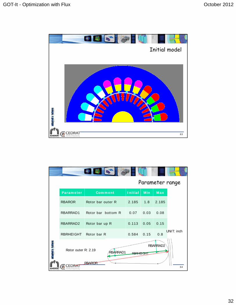
Initial model

64

Parameter range

Parameter Comment Initial Min Max

RBAROR Rotor bar outer R 2.185 1.8 2.185

RBARRAD1 Rotor bar bottom R 0.07 0.03 0.08

RBARRAD2 Rotor bar up R 0.113 0.05 0.15

RBRHEIGHT Rotor bar R 0.584 0.15 0.8UNIT: inch

RBRHEIGHT

RBARRAD2

RBARRAD1

RBAROR

Rotor outer R: 2.19


33

65

Screening

Box 16

Taguchi 9

Box 8

66

Fixed RBAROR

Box 8 only


34

67

Start optimization for lock rotor

Fixed RBAROR and RBARRAD1

68


35

69

Parameter range

Parameter Comment Initial Min Max final

RBAROR Rotor bar outer R 2.185fixed

RBARRAD1 Rotor bar bottom R 0.07

RBARRAD2 Rotor bar up R 0.113 0.05 0.15 0.0618

RBRHEIGHT Rotor bar R 0.584 0.15 0.8 0.222

UNIT: inchRBRHEIGHT

RBARRAD2

RBARRAD1

RBAROR

70

Geometry optimized for locked rotor condition


36

71

Current density

72

Copper

Aluminum


37

73

Optimization case2 multi objective

Decrease rotor yoke iron depth to make machine lighter.

Also keep the flux density in rotor yoke under saturation.

Add a parameter RBI (yoke iron depth)

74

RBI


38

75

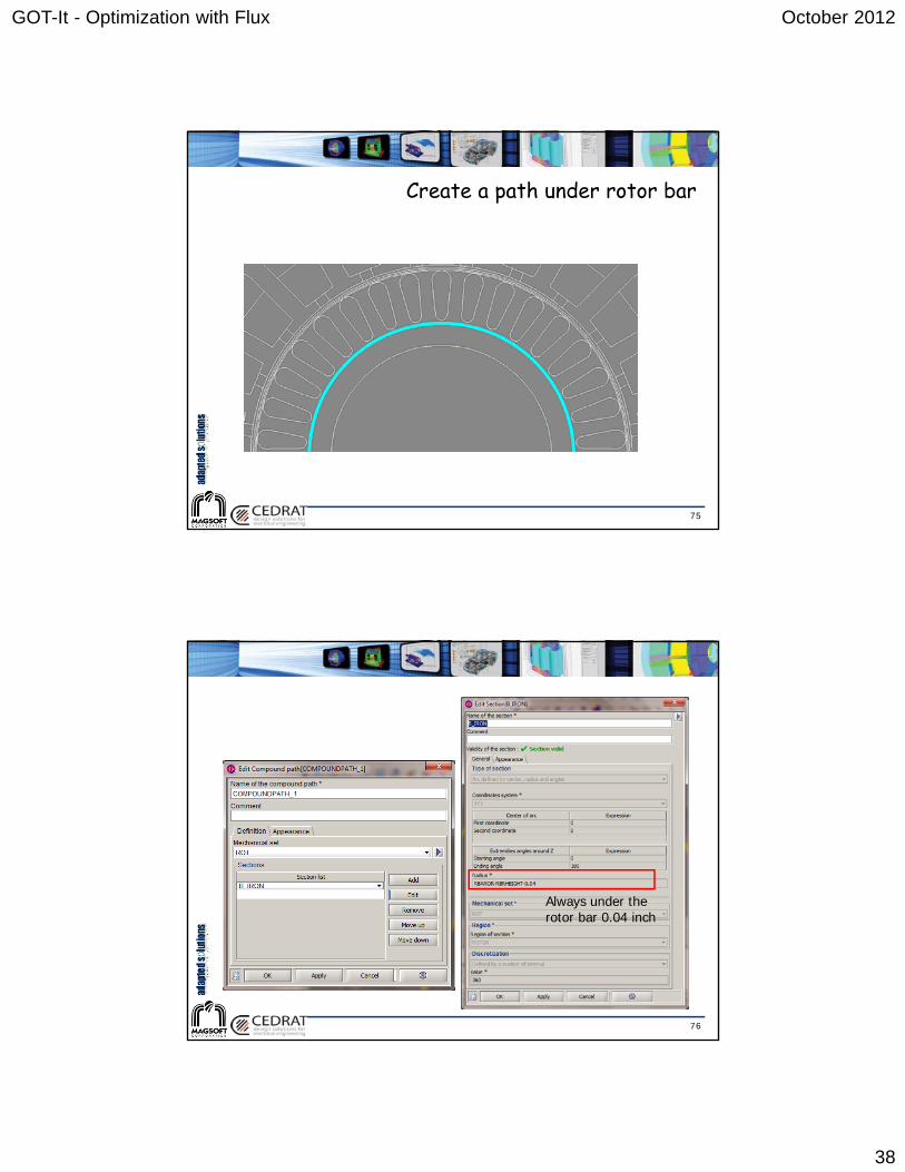
Create a path under rotor bar

76

Always under the rotor bar 0.04 inch


39

77

78

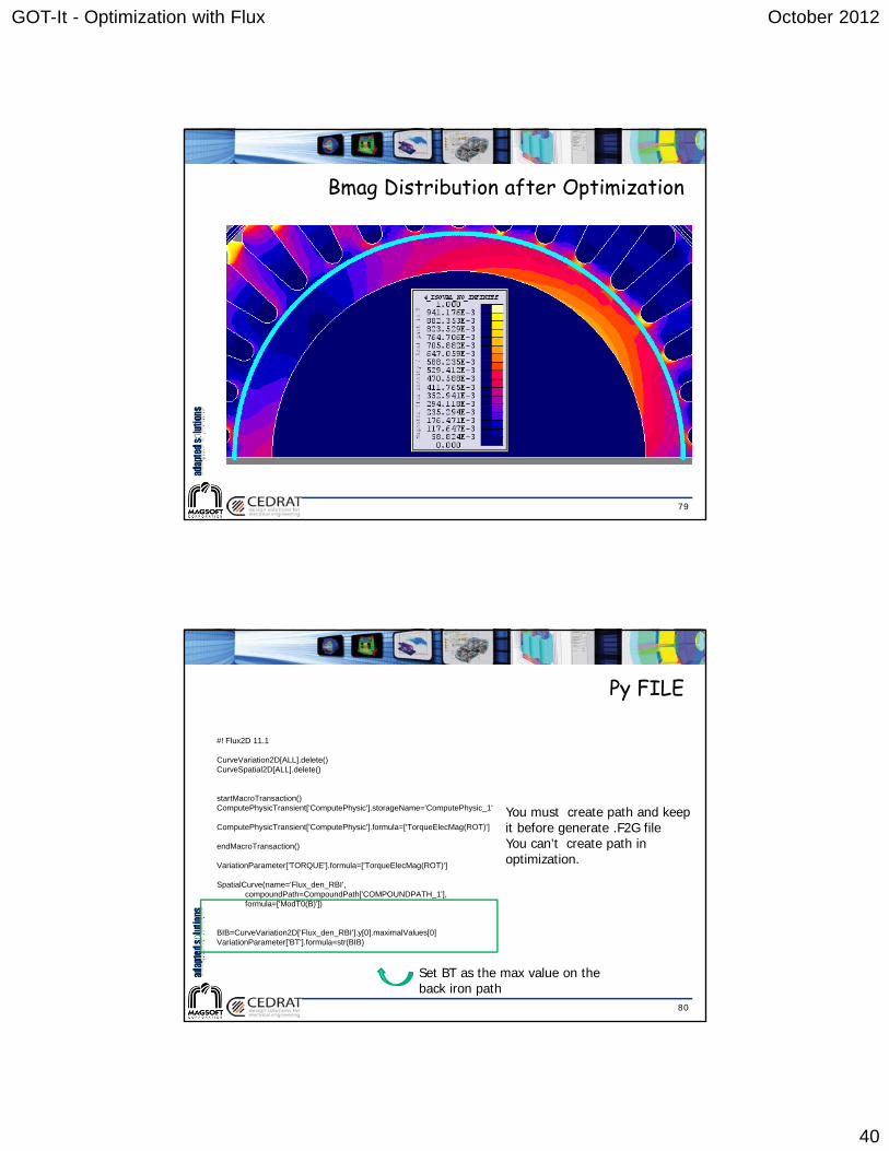
Flux Density in Rotor Yoke


40

79

Bmag Distribution after Optimization

80

Py FILE

#! Flux2D 11.1

CurveVariation2D[ALL].delete()CurveSpatial2D[ALL].delete()

startMacroTransaction()ComputePhysicTransient['ComputePhysic'].storageName='ComputePhysic_1'

ComputePhysicTransient['ComputePhysic'].formula=['TorqueElecMag(ROT)']

endMacroTransaction()

VariationParameter['TORQUE'].formula=['TorqueElecMag(ROT)']

SpatialCurve(name='Flux_den_RBI',compoundPath=CompoundPath['COMPOUNDPATH_1'],formula=['ModT0(B)'])

BIB=CurveVariation2D['Flux_den_RBI'].y[0].maximalValues[0]VariationParameter['BT'].formula=str(BIB)

You must create path and keep it before generate .F2G fileYou can’t create path in optimization.

Set BT as the max value on the back iron path


41

81

Parameter range


RBARRAD2 Rotor bar upR 0.113 0.05 0.15 0.0618

RBRHEIGHT Rotor bar R 0.584 0.15 0.8 0.222

RBI Rotor backiron depth 0.3 0.2 0.7 0.239

UNIT: inch

RBRHEIGHT

RBARRAD2

RBARRAD1

RBAROR

82

Objective functions

1. the same lock rotor torque.

2. decrease the rotor back iron depth


42

83

Add constraints

84


43

85

Flux density at slip = 0.277

86

Optimization Induction Machine 2

Change the rotor bar material from aluminum to copper.

Change the rotor bar shape to keep the same lock rotor torque as initial aluminum rotor bar.


44

87

1st Initial model Parameter range


CAGE1_SD_R Rotor bar slot depth 1.4 0.4 1.5 0.402

CAGE1_TW_R Rotor tooth width 0.25 0.2 0.3 0.2638

Copper resistivity: 2.2e-8

88

Lock rotor torque 426.317 Nm


45

89

117 iteration then interrupt

90

Torque – slip


46

91

Power balanceinput power -48677.98

speed(rpm) 1768.5

stator loss 1592.90T (Nm) 248.581rotor loss 725.86Pout 46036.4273total loss 2494.53Eff 0.9486power diff -147.02diff % -0.003020297

input power -48180.67

speed(rpm) 1761.66

stator loss 1405.64T (Nm) 246.709rotor loss 941.42Pout 45513.0253total loss 2544.01Eff 0.94706power diff ‐123.64

diff % 0.002566

input power -39990.71

speed(rpm) 1768.5

stator loss 1031.53T (Nm) 205.1822rotor loss 644.19Pout 37999.1047total loss 1872.67Eff 0.95303power diff -118.94diff % 0.002974194

Aluratedslip = 0.0175

copslip = 0.0175

copslip = 0.0213The same torque

92

Change rotor model

RB1

RB2

SDRB

RBI


47

93

2nd optimization for locked rotor torque

94

Parameter range 8 iteration interrupt


RB1 Rotor bar top radius 0.143 0.06 0.17 0.0912

RB2 Rotor bar bottom radius 0.05 0.01 0.11 0.0294

4

SDRB Rotor bar slot depth 1.1633 0.1 1.3 0.803


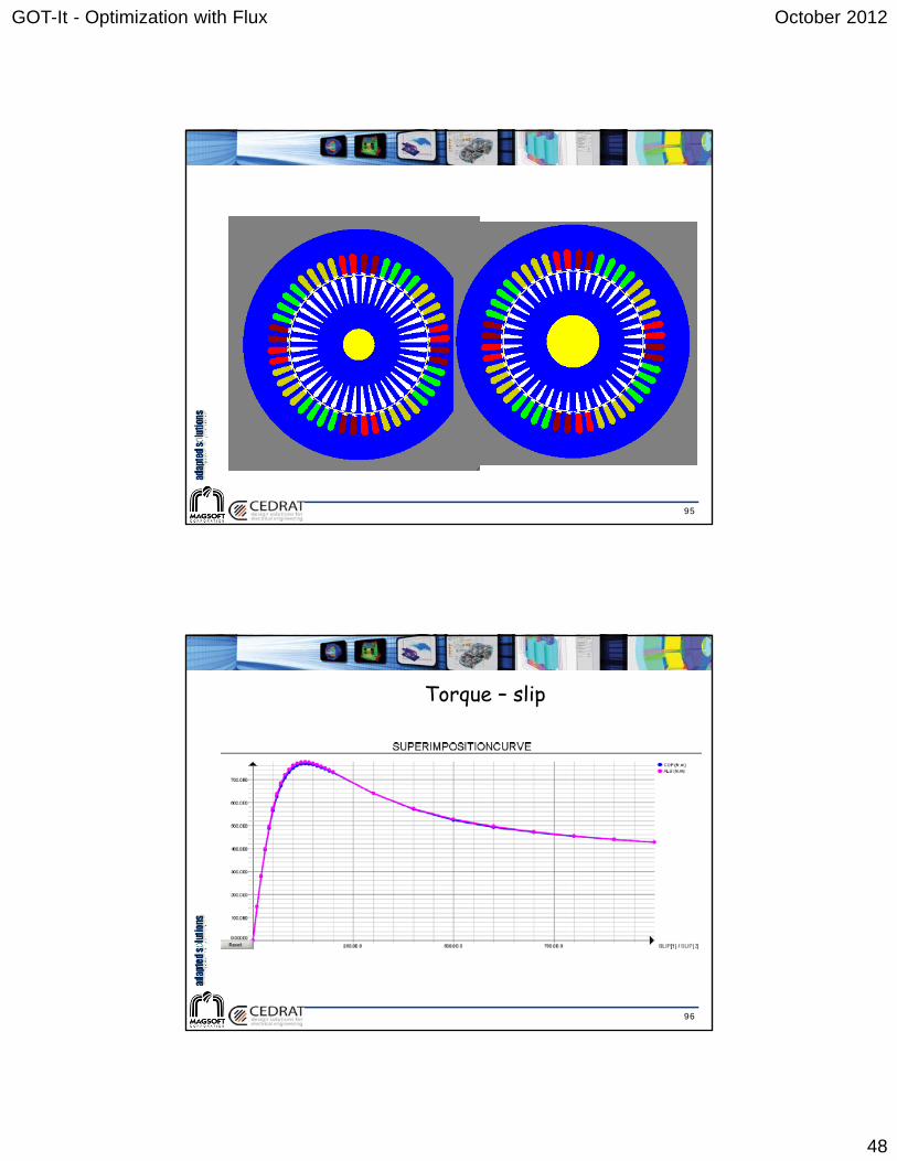
Torque - 426.184 Nm only 0.13 Nm difference with Alufor 9-hr solving period time


48

95

96

Torque – slip


49

97

Power balanceinput power -48677.98speed(rpm) 1768.5stator loss 1592.90T (Nm) 248.581rotor loss 725.86Pout 46036.4273total loss 2494.53Eff 0.9486power diff -147.02Rotor bar area(mm2) (each) 173.8

diff %

-0.00302029

7Rotor iron area(mm2) (1/4) 4446

input power -48384.68speed(rpm) 1768.5stator loss 1435.74T (Nm) 247.0765rotor loss 765.86Pout 45757.7986total loss 2397.72Eff 0.95021power diff -229.16Rotor bar area(mm2) (each) 73.1

diff %0.0047362



copslip = 0.0175

98

3rd optimization for rated speed rotor torque


50

99

Parameter range


RB1 Rotor bar top radius fixed 0.0912

RB2 Rotor bar bottom radius

0.02944 0.01 0.11 0.1031

SDRB Rotor bar slot depth 0.803 0.1 1.3 1.19

RBI Rotor back iron depth 1.3 0.7 2 0.424


Torque – 248.524 Nm only 0.057 Nm difference with Alu

100

Py FILE

#! Flux2D 11.1

CurveVariation2D[ALL].delete()CurveSpatial2D[ALL].delete()

startMacroTransaction()ComputePhysicTransient['ComputePhysic'].storageName='ComputePhysic_1'

ComputePhysicTransient['ComputePhysic'].formula=['TorqueElecMag(ROT)']

endMacroTransaction()

VariationParameter['TORQUE'].formula=['TorqueElecMag(ROT)']

SpatialCurve(name='Flux_den_RBI',compoundPath=CompoundPath['COMPOUNDPATH_1'],formula=['ModT0(B)'])

BIB=CurveVariation2D['Flux_den_RBI'].y[0].maximalValues[0]VariationParameter['BT'].formula=str(BIB)

You must create path and keep it before generate .F2G fileYou can’t create path in optimization.

Set BT as the max value on the back iron path


51

101

Obj functions

1. the same rated speed torque.

2. decrease the rotor back iron depth

102

Add constraints


52

103

Optimization algorithm – GMGAfor multi-obj.

104


53

105

106


54

107

108


55

109

110


56

111

Co lock rotor torque :370.428 Nm

Alu lock rotor torque : 426.314 Nm

112

Power balanceinput power -48677.98speed(rpm) 1768.5stator loss 1592.90T (Nm) 248.581rotor loss 725.86Pout 46036.4273total loss 2494.53Eff 0.9486power diff -147.02Rotor bar area(mm2) (each) 173.8

diff %

-0.00302029


input power -48661.38speed(rpm) 1768.5stator loss 1448.37T (Nm) 248.524rotor loss 769.87Pout 46025.8711total loss 2414.33Eff 0.95015power diff -221.19Rotor bar area(mm2) (each) 73.5

diff %0.0045453



copslip = 0.0175


57

113

Flux density between 1 T and 2 Tat lock rotor

114

Flux density between 1 T and 2 Tat rated speed


58

115

Current density at lock rotor

116

Thank you for your interest in our modelling solutions

www.magsoft-flux.com

[email protected]@[email protected]

create, design, engineer! - 北京天源博通科技有限公 … winding copper losses motor drive...

Documents