Institute of Transportation StudiesUniversity of California at Berkeley

July 2005ISSN 0192 4095

RESEARCH REPORTUCB-ITS-RR-2005-5

Crane Double Cycling in Container Ports: Effect on Ship Dwell Time

Anne V. Goodchild and Carlos F. Daganzo

Crane Double Cycling in Container Ports: Effect on Ship Dwell Time

Anne V. Goodchild, Carlos F. Daganzo Department of Civil and Environmental Engineering, University of California, Berkeley, CA 94720,

{anne_g@berkeley.edu, daganzo@ce.berkeley.edu}

Loading ships as they are unloaded (double-cycling) can improve the efficiency of a quay crane and thus container port. This paper describes the double-cycling problem, and presents two solution algorithms and simple formulae to estimate reductions in the number of operations, and operating time.

The problem is formulated as a scheduling problem. Small problems can be solved to optimality with a standard numerical solver, but problems of typical size are computationally burdensome and terminated after 10 hours with optimality gaps larger than 50%. A formula for an improved lower bound to the optimal solution is developed and shows the optimality gaps are actually below 2.5% in all cases.

The paper presents a greedy algorithm that can obtain solutions in seconds. A formula for an upper bound to the greedy algorithm’s performance can be used to accurately predict crane performance.

The problem is extended to include an analysis of double-cycling when ships have deck hatches. Results are presented for many simulated vessels, and compared to empirical data from a real-world trial. The paper demonstrates that analytical methods can be used in addition to numerical methods to provide greater insight. More importantly, the paper demonstrates that double-cycling can create significant efficiency gains.

Key words: logistics, freight transportation, terminal operations, container port terminal

Introduction The volume of goods moved by container through the US transportation system has grown dramatically over the last 15 years, but our infrastructure has not. This has led to significant freight congestion at transportation terminals, and greater interest in freight from governmental planning agencies. Strategies are required that aid the movement of freight through the system, and specifically through terminals. Quay cranes are the most expensive single unit of handling equipment in port container terminals, and because of this, one of the key operational bottlenecks at ports is quay crane availability (Crainic and Kim 2004). By improving quay crane utilization, ports can reduce ship turn-around time, improve port productivity and improve throughput in the freight transportation system. This work addresses the key bottleneck to port productivity; quay crane utilization.

Double-cycling is a technique that can be used to improve the utilization of quay cranes by converting empty crane moves into productive ones. Instead of using the current method, where all relevant containers are unloaded before any are loaded (single-cycling), containers are loaded and unloaded simultaneously (see Fig. 1). This allows the crane to carry a container while moving from the apron to the ship (one move) as well as from the ship to the apron; doubling the number of containers transported in a cycle (or two moves). This crane efficiency improvement can be used to reduce ship turn-around time and therefore improve port throughput, and address the capacity problem.

In their efforts to increase productivity, ports have undertaken various projects such as renovating and adding terminals, constructing and expanding intermodal facilities, and implementing new IT infrastructure (Mangelluzzo 2005). Because crane productivity is so important, ports have also invested in various crane utilization improvement strategies. For example, dual hoist cranes have been developed that separate the crane’s cycle into two subcycles that can be operated independently. These are currently in use at many ports, including Rotterdam and Norfolk. Operational changes are of interest because they provide benefits at less cost. The concept of double-cycling is recognized by some in the industry (Ward 2005), (Yau 2003), and its potential to improve efficiency is intuitively understood. Although small scale trials have been undertaken at San Pedro and Tacoma, as well as at ports in Asia and Europe, a broad implementation of double cycling has not occurred. There are several reasons for this. First, small scale trials have understated the benefits of double cycling which, as we will show, increase with the number of containers. Second, the lack of implementation tools that detail the necessary operational changes leave some operators doubting that the benefits will overcome the operational costs. Third, the absence of a rigorous analysis of the benefits of double cycling leaves the question of its impact on crane operations open. This paper aims to address this final point by providing a quantitative analysis of the impact of double cycling on crane efficiency. We emphasize this point through comparison with empirical data.

To address point two, we will assume the ship’s loading plans are given. Creating vessel

loading plans is a complicated process, with many competing objectives. Shipping lines use software tools to create loading plans that accommodate vessel stability requirements, placement constraints on hazardous materials, refrigerated containers, above, and below deck storage, and may include strategies to minimize the number of cycles necessary to unload containers at subsequently visited ports. From these tools, a sequence of operations is generated for the crane operator and foreman (who directs landside operations). When

considering the benefits of double cycling, this paper assumes that existing planning tools have been used to create a loading plan, as is current practice, and that this loading plan has made no accommodations for double cycling. We therefore consider changes only to the crane’s sequence of operations. In practice, this would be determined at a planning stage, and the crane operator would be given a sequence of operations to carry out, in the same way they are when performing single-cycle operations. This way we may demonstrate that double-cycling is feasible and beneficial without disrupting current operations.

Although no academic research has addressed the problem of double cycling, a significant

amount of research has addressed other problems of port design and operation. Port research typically focuses on strategic design planning issues such as the number of berths (Schonfeld and Sharafeldien 1985), the size of storage space (Kim and Kim 2002), and the number of various pieces of equipment to install (Vis et al 2001). Operational planning and control problems include berth scheduling (Park and Kim 2003), quay-crane scheduling (Daganzo 1989), stowage planning and sequencing (Christiansen et al 2004), storage space planning (Castilho and Daganzo 1993), and dispatching of yard cranes and prime movers (Kim and Bae 1999). To date, most of this work utilizes queueing theory and stochastic models (Daganzo 1990), simulation (Lai and Leung 2000), and classical operations research techniques such as routing, network, and scheduling problems (Kim and Kim 2002).

In the next section, a framework is set for analysis of the problem. The section also includes an example that is used to illustrate the problem’s basic properties. In Section 2 a scheduling formulation, and the results from its implementation with a numerical solver are presented. A lower bound to the problem is developed in Section 3. Section 4 presents a new algorithm and bounds its results. The problem is extended to accommodate ships with deck hatches in Section 5. Section 6 presents the results of simulated vessel loadings and unloadings, tools to convert benefits from cycles to time, and compares time-savings to empirical results. The paper concludes with a discussion.

1. Modeling Framework The layout of containers on a ship can be modeled as a 3-dimensional matrix. Containers are stacked on top of one another, and arranged in rows. One row stretches across the width of the ship. Large container vessels today typically hold 20 stacks of containers across the width of the ship, and up to 20 stacks along the length of the ship (40-foot equivalent units). Of course, we expect these figures to increase with the penetration of Malacca-max carriers. Figure 2 gives a top and side view of a typical vessel (although the number of container stacks is not representative). The complete operating cycle of the crane can be broken down into the following components;

a) locking to or unlocking from a container, b) lengthwise motion along the ship, c) horizontal motion across the ship, d) vertical motion.

It is important to point out that the number of locking and unlocking operations is not affected by double cycling. The same number of containers will need to be picked up and put down

with single or double cycling. In this research we will assume that dockside containers are ready for loading when required, and containers being unloaded can be quickly removed from the immediate area. In the initial analysis it will be assumed that ships lack hatch-coverings, or doors on the deck that separate above-deck and below-deck storage. This assumption will be relaxed in Section 5.

Consider the case where a ship arrives in port with a set of containers on board to be

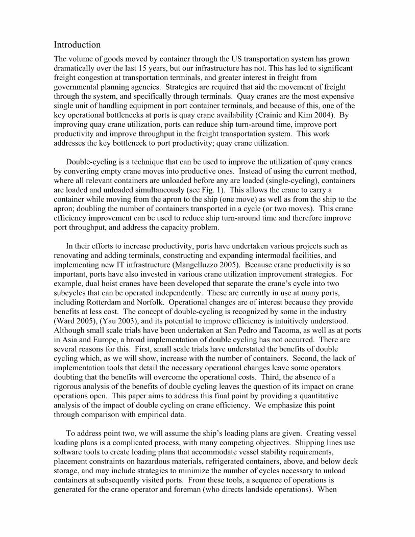
unloaded and a loading plan for containers to be loaded. The loading plan indicates the placement of containers on the ship. Given are uc and lc, the number of containers to be unloaded and loaded, respectively, in each stack labeled c. Figure 3 is an example problem that will be used for illustrative purposes. A rehandle is a container than must be moved to access containers below it, but will then be stowed again before the ship departs. Note that if any rehandles are necessary, these are included in the total number of loads and unloads. Note that this will over-estimate the amount of work necessary to unload and load a set of containers because the container is considered moved from the vessel to the shore and back to a location on the vessel. In Fig. 3, uA = 3 and lA = 2.

The set of stack labels, c, is called S. An ordering of these stacks can be described by a permutation function, Π. A permutation is a one-to-one correspondence between the set of n ∈ {1,…, N} and c ∈ S such that Π(n) = c, or n = Π-1(c). For example, in Fig. 3, the set of stack labels S = {A, B, C, D} a permutation of these is {B, A, C, D} given by the function Πe where Πe(1) = B, Πe(2) = A, Πe(3) = C, and Πe(4) = D.

If we consider the time it takes to unload and load a ship to be a measure of crane productivity, then the goal of double cycling is to reduce the total turn-around time. A proxy for this is the number of cycles. We will discuss time-savings in section 7. The number of cycles necessary to complete loading and unloading will be represented by the variable w. We will consider double cycling whithin one row of the ship. We will complete unloading and loading of one row before moving the crane lengthwise along the ship to the next row. Thus we will not require the crane to move laterally along the ship within one cycle. We will restrict our attention to special cases of the generic double-cycling method described below:

• Choose an unloading permutation, Π′ . Unload all containers in the first stack of the permutation, then all containers in the second stack of the permutation, proceed in this fashion until all stacks have been unloaded.

• Choose a loading permutation, Π, and load the stacks in that order. Load all containers in the first stack, then in the second, etc.. Loading can start in any stack as soon as it is empty or it contains just containers that should not be unloaded at this port. Once loading has begun in a stack, continue loading until that stack is complete.

Figure 4(a) is a queueing diagram for a single-cycling operation where the stacks of Fig. 3

are handled in the order {A,B,C,D} both for loading and unloading. Time is expressed in cycles. Note that loading operations must wait until cycle w = 10, when unloading is finished. The process requires w = 20 cycles.

If we double-cycle, we can still plot the unloading curve on the same diagram. Now, using the same sequence for unloading and loading, Π′= Π = {A,B,C,D}, we can shift the

loading curve to the left as far as possible without overlapping the unloading curve. Figure 4(b) shows the maximum shift. Loading can start as early as w = 4 and the process would require only 14 cycles. The same number of cycles is obviously obtained if we start loading each stack as early as possible, as in Fig. 4(c). This introduces some delay as the loading operations must wait one cycle for the unloading operations to be completed in stack B, but does not change the completion time.

With single-cycling one cycle is required for every container. With double-cycling, however, the number of cycles will depend on the sequence. Fig. 4(d) shows that if the loading and unloading sequence is {B,A,C,D}, then the completion time is w = 13.

In the next section we formulate the problem of determining Π′ and Π as a mixed integer program and discuss the results of its implementation using a numerical solver.

2. Scheduling Approach The problem is formulated as a job shop scheduling problem where jobs are equated with the loading or unloading of stacks and the crane operates as two machines . Since all work on loading and unloading is assumed to be continuous, we just look for the job completion times. Start times are identified from the known job durations. We use the following notation:

uc - number of containers to unload in stack c ∈ S lc - number of containers to load in stack c ∈ S Xc - completion time, i.e. cycles, of unloading c ∈ S Yc - completion time of loading c ∈ S w - total completion time Xkj - binary variable to track ordering of unloading jobs (1 if j ∈ S is unloaded after k ∈ S and 0 otherwise) Ykj - binary variable to track ordering of loading jobs (1 if j ∈ S is loaded after k ∈ S and 0 otherwise) M - a large number

The scheduling problem (SP) is to minimize the completion time of all jobs subject to

constraints that uniquely identify the permutations Π and Π′ , and a feasible set of job start and end times. It is assumed that the process starts at time zero. The formulation is: minimize w subject to w ≥ Yc ∀c ∈ S, (1a) Yc – Xc ≥ lc ∀ c ∈ S, (1b) Xk – Xj + MXkj ≥ uk ∀j,k ∈ S, (1c) Xj – Xk + M(1-Xkj) ≥ uj ∀j,k ∈ S, (1d) Yk – Yj + MYkj ≥ lk ∀j,k ∈ S, (1e) Yj – Yk + M(1-Ykj) ≥ lj ∀j,k ∈ S, (1f) Xc ≥ uc ∀c ∈ S, (1g) Xkj, Ykj = 1, 0 ∀j,k ∈ S. (1h)

These constraints completely define the double-cycling problem. Constraints (1a) ensure that the process ends when the last stack is loaded or later. Constraints (1b) ensure that stacks are only loaded when empty. Constraints (1c), (1d) and (1h) ensure that every stack is unloaded after the previous one in Π′ has been unloaded. This is achieved by specifying for every pair of stacks (j,k) that either stack k is unloaded before stack j (if Xkj = 1) or the reverse (if Xkj = 0), and that the time difference between the two events is large enough to unload the second of the two stacks. Constraints (1e), (1f) and (1h) are equivalent to (1c), (1d) and (1h) but for loading jobs. Constraints (1g) ensure that each unloading completion time allows for enough time to at least unload that stack.

The SP is in the family of job shop scheduling problems. These problems are notoriously difficult to solve. Heuristic solution algorithms have been developed for some versions. For a summary of current solution techniques see Pinedo (2002), or Applegate and Cook (1991). These methods are not readily applicable to the SP. In our problem, there are two machines; an unloading crane and a loading crane (in reality this is one device). Each stack must visit the unloading crane before the loading crane, and containers are only loaded into stacks from which all relevant containers have been unloaded.

Ship data were generated to evaluate the algorithm. The numbers of containers to load and unload in each stack were assumed to be independent and uniformly distributed between 0 and 10. A standard numerical solver (AMPL with CPLEX 8.0) was then used to determine the optimal permutation. Table 1 shows the number of stacks, solution time, number of runs, and optimality gap. Runs were carried out on a 1.4 MHz Dell Poweredge 1650 server, running Linux with 2 GB of real memory and 1 GB of swap space.

For small problems (10 stacks and fewer), the problem could be solved optimally. However, average solution times were found to grow quickly with problem size (number of stacks). Problems with more than 10 stacks (about half the size of typical problems) could not be solved optimally in less than 10 hours. The optimality gaps of Table 1 are the percent difference between the solution at ten hours and the highest lower bound known. The highest lower bound known is the solution to an infeasible relaxation to the problem. For example, if the solution was 100 cycles, and the highest lower bound known 75 cycles, then the optimality gap would be 25%. These gaps increased with problem size and were rather large, even for N = 15, so the quality of the 10-hour solutions were uncertain.

This shows that, for small problems, the numerical solver provides a good solution. For typical problems however, further analysis is desirable.

3. Lower Bound We will now determine a lower bound for the number of cycles, which can be used to better judge the quality of the numerical solver’s solutions. Define:

∑∑∈=

Π′ ==Sc

c

N

nn uuY

1)( , ∑∑

∈=Π ==Λ

Scc

N

nn ll

1)( .

Recall from Fig. 4(a) that using single-cycling, the number of cycles necessary to

complete a row is:

Υ + Λ.

This is intuitive; one cycle for each container. We have assumed the crane must start and

finish on the dock.

For double-cycling, with a specific loading permutation Π and unloading permutation Π′ , the number of cycles must be at least )1('Π+Λ u which satisfies:

)(min)1(' cc uu +Λ≥+Λ Π . (2)

The right-hand side of (2) is a general lower bound that applies to all permutations. It is also a lower bound if we force the same permutation for loads and unloads (Π′ = Π). More specifically, if w1

* is the optimal number of cycles with the same permutation for loading and unloading and w2

* is the optimal number of cycles with different permutations, we can write:

)(min*2

*1 cc uww +Λ≥≥ . (3)

1. The new lower bound reveals that the quality of the solution determined by the

numerical solver (in 10 hours) is quite high. Revised optimality gaps, using (3) for the lower bound, are given in Table 2.

Currently, rows do not accommodate more than 20 stacks, but it is useful to understand the behavior of the algorithm across a range of problem sizes. Vessels will continue to grow in size, and, in addition, technologies may change to allow for more efficient lateral movement of the crane. This is why our results were extended to 250 stacks. For current vessels, the generic algorithm is not fast enough to be used for real-time applications. Therefore, we will discuss an alternative algorithm that can be used for real-time applications, that is simpler, and provides greater flexibility and insight. The algorithm yields an upper bound formula for the required number of cycles. The formula can be evaluated without running the algorithm, and thus is useful for planning purposes.

4. Greedy Strategy and an Upper Bound We propose to unload and load each stack as soon as possible, assuming that the loading and unloading sequences are given by the same “greedy” permutation, Π′= Π = G. This greedy permutation is obtained by ordering the stacks in descending order of the variable dc where:

dc = lc – uc )( Υ≥Λif , (4a) dc = uc – lc )( Υ<Λif . (4b)

The rationale for (4a) is that we want the unloading operations to run ahead of the loading

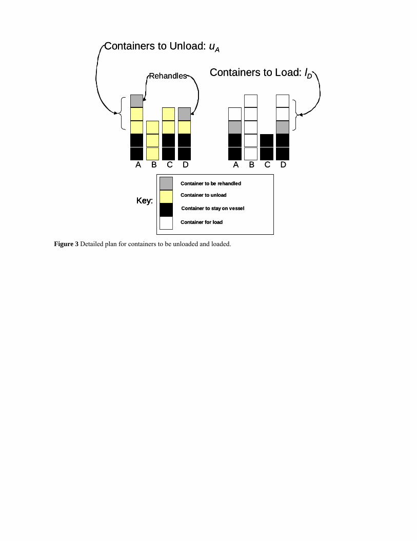
operations as much as possible. We will now introduce some terminology which will allow us to prove the existence of an upper bound on the number of cycles required using the greedy strategy. Associated with this strategy, we define functions U(w) and L(w) for the number of stacks completed as illustrated by the solid curves on the top and bottom parts of Fig. 5. We

also define L-1(c) and U-1(c) for integer c as the inverse functions, and Uc = uG(c) and Lc = lG(c)

as the horizontal steps of the curves. See Fig. 5 and the notations along the bottom of the abscissa’s axis. Note that U(Y) = L(Λ) = N. Define wG as the number of cycles with G. THEOREM 1. If Λ ≥ Y, then )(max)(min *

1*2 ccGcc uwwwu +Λ≤≤≤≤+Λ .

PROOF. In view of (3), it suffices to prove )(max*

1 ccG uww +Λ≤≤ . Since *1wwG ≥ it suffices to show that Gcc wu ≥+Λ )(max . Consider a horizontal shift, L,

to curve L, that will ensure curve L is to the right of curve U (as in the dotted curve in the top of Fig. 5), i.e. that L-1(c-1) + L ≥ U-1(c) for c = 1,... N. Obviously the least possible delay, L0, is maxi(U-1(c) – L-1(c-1)) = maxc(Uc + (U-1(c-1)-L-1(c-1)). Since Λ ≥ Y, the greedy strategy satisfies (U-1(c-1) – L-1(c-1)) ≤ 0 ∀ c. Hence L0 ≤ maxc(Uc). Therefore maxc(Uc) + Λ = )(max cc u+Λ is an upper bound to the number of cycles. □ COROLLARY 1. If Λ ≤ Y, then )(max)(min *

1*2 ccGcc lwwwl +Υ≤≤≤≤+Υ .

PROOF. G in this case is defined by (4b). That Corollary 1 is true should be

obvious by symmetry. If one were to record the process of unloading and loading the row, and then play this recording in reverse, the reversed movie would display a sequence of operations with the same total time as for a problem in which the role of loads and unloads is switched. Thus, for every problem instance with loads greater than unloads, there is a dual instance where unloads are greater than loads. Figure 6(b) shows the reverse movie of Fig. 6(a). Note that the greedy strategy continues to be greedy in reverse, and that everything said up to this point, including the bounds, continues to hold with time running backward. Note that in Fig. 6(b) the greedy strategy with time running backward implies a reverse ordering of {dc}, as specified in (4b), thus Corollary 1 holds. □

Define )(max),(max),(min),(min **cccccccc llanduulluu ===′=′ . Then given

Theorem 1 and Corollary 1 we can write:

),max(),max( ***1

*2 luwwwlu G +Υ+Λ≤≤≤≤′+Υ′+Λ . (5)

For rows of large ships where (Λ,Y) >> (u*, l*), the greedy strategy is very close to both

the upper and lower bounds since all the members of (5) are relatively close to max(Λ,Y). More specifically, note that if uc and lc are bounded by a constant (stack size) then the percent optimality gap vanishes as the number of stacks (problem size) tends to infinity. Thus the greedy strategy is asymptotically optimal.

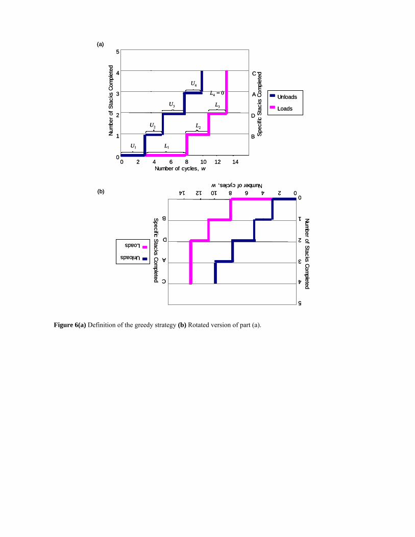
Figure 7 compares the performance of the scheduling and greedy algorithms. The percentage difference between each strategy’s solution and the minimum is shown. In general, both algorithms perform well. As expected, the greedy algorithm’s performance improves with row size. With the scheduling problem we could not provide an upper bound formula for the savings that double-cycling would provide over single-cycling. Using the

greedy strategy, we have been able to quantify the improvements double-cycling provides in all cases. Results for the greedy strategy are comparable to those of the scheduling algorithm (slightly better for the largest problems), but can be obtained more quickly. In the next section, we consider deck hatches as an extension to the problem considered so far.

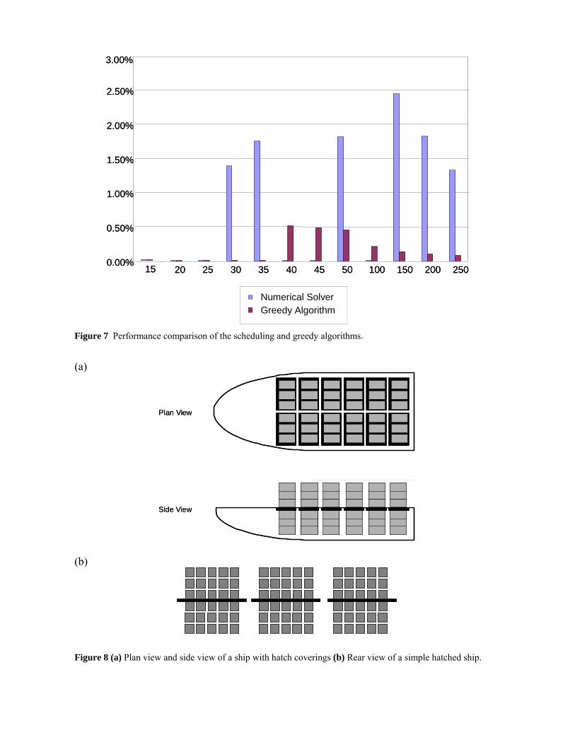
5. Deck Hatches Most container ships currently have hatch coverings, as shown in Figure 8. These are large steel plates that separate above-deck and below-deck storage. In Fig. 8(a) we have shown a vessel two hatches wide, with three stacks of containers above and below each hatch. In Fig. 8(b) we have shown a vessel three hatches wide, with five stacks above and below each hatch. Typical ships are three hatches wide, each hatch containing 5 or 6 stacks of containers. Hatches change the nature of the problem already addressed because the stacks are no longer independent. To access the containers below a hatch all containers must be unloaded from above the hatch, and before loading containers atop a hatch all containers below the hatch must be loaded.

The following algorithm (the greedy hatch strategy) will be considered. As in the hatchless case, assume that each stack on the ship is given an initial label. To carry out the strategy it is necessary to: 1. Order the hatches using a greedy strategy using the same method as for the hatchless

case. Treat the hatches as stacks, considering only the containers atop the hatches.

2. Order the stacks within each hatch using a greedy strategy, considering only the containers below deck.

The algorithm is then carried out as follows:

1. Apply the greedy strategy to the containers above deck, treating hatches as stacks,

pausing each time all containers above hatch h have been removed.

2. During the hth pause, unload and load the containers below the hth hatch using double-cycling.

As with the hatchless case, this method may not provide the least number of cycles to

complete loading and unloading operations on the row. The value of the method is its simplicity; parts of the unloading and loading process are equivalent to the hatchless ship problem already addressed. Each piece below a hatch is equivalent to a hatchless ship, and the containers above a hatch to a stack of a hatchless ship. These relationships will allow us to use the analysis of the hatchless ship to develop bounds for the hatched case. First it is necessary to define some notation. h – hatch label Sh – the set of stacks for hatch h Nh – the number of stacks of hatch h H – the set of hatches F – the number of hatches

hcu – the number of containers to unload below hatch h in stack c ∈ Sh hcu – the number of containers to unload above hatch h in stack c ∈ Sh

hcl – the number of containers to load below hatch h in stack c ∈ Sh hcl – the number of containers to load above hatch h in stack c ∈ Sh ∑

∈

=hSc

hch uu – containers to unload below hatch h

∑∈

=hSc

hch uu – containers to unload above hatch h

∑∈

=hSc

hch ll – containers to load below hatch h

∑∈

=hSc

hch ll – containers to load above hatch h

∑∑

∈ ∈

=Hh Sc

hc

h

uY – containers for unloading below deck

∑∑∈ ∈

=Hh Sc

hch

uY – containers for unloading above deck

∑∑∈ ∈

=ΛHh Sc

hc

h

l – containers for loading below deck

∑∑∈ ∈

=ΛHh Sc

hch

l – containers for loading above deck

wA = the number of cycles above deck wB = the number of cycles below deck wB,h = the number of cycles below hatch h

Also define the greedy permutation for hatches; P(f) = h; P-1(h) = f for f = 1... F; h∈H

and the greedy permutation for containers below hatch, h∈H: Π(n⏐h) = c∈Sh; Π-1(c|h) = n for c∈Sh, {n = 1...Nh}

THEOREM 2. An upper bound on the optimum number of cycles for the hatched case is },{max},{max},max{},max{ hchcSchhh

Hhhh lululu

h∈∈

++ΥΛ+∑ .

PROOF. We know from (5) that wA = number of cycles for a row of F stacks with

data given by {uh,lh} ≤ max{Λ,Y} + maxh{uh,lh}. Likewise wB =∑

∈HhhBw , =∑

∈Hh(number of cycles for a row of Nh stacks with data given by

},{ hchc lu ) ∑∈

∈+≤Hh

hchcSchh luluh

},{max},max{ . Obviously then, the total number of

cycles with the algorithm satisfies wA+ wB ≤ },{max},{max},max{},max{ hchcSchhh

Hhhh lululu

h∈∈

++ΥΛ+∑ . □

THEOREM 3. A lower bound on the optimum number of cycles for the hatched case is },{min},{min},max{},max{ hchcSchhh

Hhhh lululu

h∈∈

++ΥΛ+∑ .

PROOF. We know from (5), but treating each hatch as a stack, that the lower

bound on the number of cycles above deck is },{max},max{ hhh lu+ΥΛ . We also know from (5), but treating each hatch as a vessel, that the lower bound on the number of cycles below deck is },{max},max{ hchcSc

Hhhh lulu

h∈∈

+∑ . □

Clearly, for rows where },max{},max{ ΥΛ+∑

∈Hhhh lu >> },{max},{max hchcSchhh lulu

h∈+ ,

both the upper and lower bounds are close to the solution provided by the greedy strategy and },max{},max{ ΥΛ+∑

∈Hhhh lu provides a reasonable estimate of the total unloading and

loading time for one row. As with the hatchless case, the gap between the upper and lower bound is quite small, and decreases with the size of the row. Thus, the simple greedy algorithm is reasonably efficient.

If one only double-cycles below deck, as is current practice, the benefits of double-cycling will be reduced by roughly the ratio of containers above deck to containers below deck.

6. Evaluation This section addresses the magnitude of double cycling benefits. We present simulation results that estimate benefits in cycles for rows of current vessels. We also present tools to convert benefits from number of cycles to an amount of time, and compare these tools to data collected in a real-world trial of double cycling.

6.1 Simulation Results

To understand the benefits on a larger scale, a simulation program was developed to generate ship data for many vessels and calculate the number of cycles necessary to complete operations in each row using various double cycling strategies. For all results shown here, double-cycling only takes place below deck. This is current practice, and matches the real-world trial at the Port of Tacoma. Loading plans were generated from sets of parameters intended to approximate the universe of actual and future ships. For more details see Goodchild (2005). Results are shown in Figure 9.

As expected, the number of cycles using double cycling is always less than single cycling. Of course, if there are no containers to load, or unload, then double cycling provides no benefit. Similarly, there exist vessel loadings where double cycling will cut the number of cycles almost by half (if we were to have no containers above deck). But, on average, there is a 21% reduction in the number of cycles when using the greedy strategy. Of course, this percentage would be greater if we could also double-cycle above deck. Each time we replace two single cycles with one double cycle, we reduce the distance traveled by the crane, and save some time.

6.2 Time-Savings

We will use the following notation. Please refer to figure 10.

W – time saved for each replacement of two single cycles by one double cycle Sr - number of cycles required to turn-around row r ∈ {1…R} using single-cycling Dr - number of cycles required to turn-around row r ∈ {1…R} using double-cycling dr - number of cycles moving two containers while operating on row r ∈ {1…R} Vh - hoist speed of the trolley when not moving a container Vl – speed of the crane when moving lengthwise along the vessel Vt –horizontal travel speed of the trolley when not moving a container dV – vertical distance from the apron to the maximum height container reaches dL – lateral distance between two rows of the vessel b – horizontal distance from landside vehicle to the edge of the vessel P –width of the vessel Tr – time required to position landside vehicle after departure of previous vehicle

For each double-cycle we save some empty-crane travel relative to the two corresponding

single cycles, but we also experience a slight landside-repositioning penalty. The time penalty, Tr, is incurred because after dropping a container for unloading onto a landside vehicle, the crane must wait for a container for loading to be positioned below the crane. With single cycling, this can be done simultaneously with other crane operations. Any minor vertical motion necessary between dropping a container on the landside vehicle and picking up the next container (to remove the trolley from the work area) will also be accounted for in this penalty.

The total distance traveled by the crane is reduced by one complete empty cycle between

the apron and the position above either the container to load or the container to unload. Of course, some horizontal and vertical motions will take place simultaneously. An upper bound on the time saved per cycle, W, is provided by summing the horizontal and vertical travel times, the lower bound by taking the maximum of the two:

( ) ( )r

tth

Vr

tth

V TV

P

Vb

Vd

WTV

P

Vb

Vd

−⎥⎥

⎦

⎤

⎢⎢

⎣

⎡+⎟⎟

⎠

⎞⎜⎜⎝

⎛>>−

⎥⎥

⎦

⎤

⎢⎢

⎣

⎡++ 3

1,max23

12 (6)

For each double cycle the vertical distance is reduced by 2dV. The horizontal distance is reduced by twice the distance between the apron and the closer of the two containers. This is

))3/1((2 Pb + , assuming a uniform distribution of locations. If double cycling only below deck, the maximum height reached while double cycling will be the clearance height of the vessel. The number of cycles saved by double-cycling in each row is dr = Sr – Dr.

After completing loading and unloading operations on a row the crane moves along the

vessel to the next row. If there are R rows on a vessel, the time consumed with lateral motion is 2*(R-1)*dL/Vl with single cycling, and (R-1)*dL/V, exactly half, with double cycling.

6.3 Validation

In June 2003, the Center for the Commercial Deployment of Transportation Technologies, Transystems, the Port of Tacoma, and Washington United Terminals, worked together on a full-scale demonstration of the Efficient Marine Terminal concept. Double cycling of container cranes is a key element of this concept and on June 28, one bay of a Hanjin vessel was loaded and unloaded simultaneously using double cycling (TranSystems Corp. 2003). Double cycling occurred below deck only. During this trial, the adjusted average time for a single cycle was 1 minute and 45 seconds, and for a double cycle, 2 minutes and 50 seconds. We now compare the difference in these empirical cycle times to the differences obtained using the expressions developed above. Parameter values based on the trial at Tacoma are given in Table 3 (Garcia, 2005).

The lower bound is 25.4 seconds. The upper bound, 39.8 seconds. The upper bound is very close to the empirical difference of 40 seconds. We expect these empirical results to better match the upper bound as we assume a constant (maximum) speed of the crane.

Clearly the specific results depend on the parameters of each crane, vessel, and container arrangement, but we have demonstrated that our tools provide results that match empirical data. A 21% reduction in the number of cycles reduces operating time by approximately 8%. A 35% reduction in cycles would reduce operating time by 13%.

We can estimate the financial benefits of double cycling by comparing productive ship

time (moving containers) to unproductive time. Intercontinental freight rates are estimated at $.045 per TEU-km (Notteboom 2004). At this rate, each hour of idle vessel time costs the ship operator $10,000. The 40 second benefit of each double cycle is worth approximately $100. During typical operations, double cycling could provide approximately $350 per hour, saving about $15,000 on a large container vessel. With three cranes per vessel, this is comparable to the total crane operator’s wages for loading and unloading the vessel.

7. Discussion Through the research presented in this paper we have developed an understanding of the impact of double-cycling on loading and unloading operations both with respect to the number of cycles, and amount of time. For very small problems an exact, optimal solution is obtained. For larger problems, a sub-optimal strategy is developed that can be solved quickly. Results for this strategy are tightly bounded by simple formulae, and comparable to results obtained after 10 hours using a numerical solver. Savings in cycles and time can be quickly calculated allowing for a flexible and transparent process.

The results obtained are applicable to a wide range of scenarios including large and small vessels, those with many or few port visits, and a varying number of cranes operating per ship. An alternative approach that focused on providing more accurate information for specific cases would require detailed information on each container. Our approach relies on only a small number of parameters, and sensitivities to these parameters are easily measured. Favorable comparisons to empirical results support our approach.

Double-cycling while unloading and loading the vessel creates an opportunity to double-cycle landside equipment. Chassis used to deliver containers to the apron can then carry an unloaded container to local storage. Typically, these chassis return to local storage empty. Future work will consider double-cycling with landside equipment in more detail. Our ongoing research focuses on addressing planning level decisions such as the impact of double-cycling on the need for landside transport vehicles, apron space, and port productivity. We are also working on designing loading plans to create more opportunities to double cycle. Finally, we would like to emphasize a key result; that any amount of double cycling will reduce the time required to turn around the vessel, at $100 per cycle the savings can be very significant. While the benefits of double cycling will not solve current port congestion they can be implemented quickly and, in conjunction with other measures, can ease congestion before more long-term infrastructure projects come on line. Acknowledgements This work has been funded in part by the National Science Foundation, Grant CMS-0313317.

References Applegate, D., W. Cook. 1991. A Computational Study of the Job-Shop Scheduling Problem. ORSA Journal on Computing 3 149-156. Castilho, B. D., C. F. Daganzo. 1993. Handling Strategies for Import Containers at Marine Terminals. Transportation Research B: Methodology 27 151-166. Christiansen, M. et al. Forthcoming. “Maritime Transportation”, in Handbooks in Operations Research and Management Science: Transportation, C. Barnhart and G. Laporte (eds) North-Holland, Amsterdam, The Netherlands. Crainic T.G., K.H. Kim. Forthcoming. “Intermodal Transportation”, in Handbooks in Operations Research and Management Science: Transportation, C. Barnhart and G. Laporte (eds) North-Holland, Amsterdam, The Netherlands. Daganzo, C.F. 1989. The Crane Scheduling Problem, Transportation Research B: Methodology 23 159-175. Daganzo, C.F. 1990. The Productivity of Multipurpose Seaport Terminals. Transportation Science 24 205-216. Garcia, B. 2005. Personal Conversations. TranSystems Corp. Goodchild, A.V. 2005. An Analysis of Double Cycling and its Impact on Port Operations. PhD Dissertation. University of California at Berkeley. Kim, K.H., J.W. Bae. 1999. A Dispatching Method for Automated Guided Vehicles to Minimize Delay of Containership Operations. International Journal of Management Science 5 1-25.

Kim, K.H., H.B. Kim. 2002. The Optimal Sizing of the Storage Space and Handling Facilities for Import Containers. Transportation Research B: Methodology 36 821-835. Lai, K.K., J. Leung. 2000. Analysis of Gate House Operations in a Container Terminal, International Journal of Modeling and Simulation 20 89-94. Mongelluzzo, B. 2005. Ports Rush to Keep Up, Journal of Commerce 6(9) 26-30. Notteboom, T. 2004. Container Shipping and Ports: An Overview. Review of Network Economics 3(2) 86-106. Park, Y.M., K.H. Kim. 2003. A Scheduling Method for Berth and Quay Cranes, OR Spectrum 25 1-23. Pinedo, M. 2002. Scheduling: theory, algorithms, and systems, Prentice Hall, Upper Saddle, N.J.. Schonfeld, P., O. Sharafeldien. (1985) Optimal Berth and Crane Combinations, Journal of Waterway, Port, Coastal and Ocean Engineering 111 1060-1072. TranSystems Corp. 2003. Efficient Marine Terminal: Full Scale Demonstration. (available at www.ccdott.org). Vis, I.F.A., R. de Koster, K.J. Roodbergen. 2001. Determination of the Number of Automated Guided Vehicles Required at a Semi-automated Container Terminal, Journal of the Operational Research Society 52 409-417. Ward, T. 2005. Personal Conversations, JWD Group. Yau, V. 2003. Personal Conversations, American Presidential Lines.

Tables and Figures

Figure 1 (a) Unloading using single-cycling (b) Unloading and loading with double-cycling.

Figure 2 Plan and side views of a simplified ship (number of containers shown not representative of typical ship size).

Double CyclingDouble-Cycling

container Unload container Unload Return

without container

Load container Load container

Unload containerUnload container

Single CyclingSingle-Cycling

(a) (b)

Double CyclingDouble-Cycling

container Unload container Unload Load

container Load container

Unload containerUnload container

Single CyclingSingle-Cycling

(a) (b)(a) (b)

ABC

container

Plan View

Side View

stack label

DEF

IHG

ABC

stackcontainer

Plan View

Side View

DEF

Container for load

Key:

Container to be rehandled

Containers to Unload: uA

Key:

Containers to Load: lDRehandles

A B C D

Key:

A B C D

Container to unload

Container to stay on vessel

Container for load

Key:

Container to be rehandled

Containers to Unload: uA

Key:

Containers to Load: lDRehandles

A B C D

Key:

A B C D

Container to unload

Container to stay on vessel

Figure 3 Detailed plan for containers to be unloaded and loaded.

D

C

B

ASta

cks

com

plet

ed

Number of cycles5 10 15 20

D

C

B

ASta

cks

com

plet

ed

Number of cycles5 10 15 20

D

C

A

BSta

cks

com

plet

ed

Number of cycles5 10 15 20

D

C

B

ASta

cks

com

plet

ed

Number of cycles5 10 15 20

Unloads Loads

(a) (b)

(c) (d)

Y

Λ

ΛuB

D

C

B

ASta

cks

com

plet

ed

Number of cycles5 10 15 20

D

C

B

ASta

cks

com

plet

ed

Number of cycles5 10 15 20

D

C

A

BSta

cks

com

plet

ed

Number of cycles5 10 15 20

D

C

B

ASta

cks

com

plet

ed

Number of cycles5 10 15 20

Unloads Loads

(a) (b)

(c) (d)

Y

Λ

ΛuB

Figure 4 Turn-around time with different methods: (a) single-cycling with ordering {A,B,C,D} unloading starts at w = 10, 20 cycles (b) double-cycling with ordering {A,B,C,D} unloading starts at w = 4, 14 cycles. (c) double-cycling with ordering {A,B,C,D} unloading starts at w = 3, 14 cycles. (d) double-cycling ordering {B,A,C,D} unloading starts at w = 3, 13 cycles.

Number of Stacks

Average CPU Solution Time in minutes (limited to 10 hours (600 minutes))

Number of runs represented

Optimality Gap

2 0.00 10 ** 3 0.00 10 ** 4 0.00 10 ** 5 0.00 10 ** 6 0.00 10 ** 7 0.02 10 ** 8 0.28 10 ** 9 3.02 10 ** 10 56.11 10 ** 15 * 1 51.35% 20 * 1 67.43% 25 * 1 76.03% 30 * 1 78.08% 35 * 1 81.03% 40 * 1 84.10% 45 * 1 85.85% 50 * 1 87.05%

100 * 1 93.80% 150 * 1 96.15% 200 * 1 97.11% 250 * 1 97.63%

Table 1 Solution time and optimality gap for ships of increasing size. ** indicates the optimal solution was obtained so optimality gap is zero. * indicates run was terminated at 600 minutes.

Number of Stacks

Solution obtained after 10 hours

Lower Bound

Difference between solution and lower bound

15 74 74 0.00% 20 96 96 0.00% 25 121 121 0.00% 30 146 144 1.39% 35 174 171 1.75% 40 195 195 0.00% 45 205 205 0.00% 50 224 220 1.82%

100 468 468 0.00% 150 754 736 2.45% 200 1005 987 1.82% 250 1221 1207 1.16%

Table 2 The difference between the 10-hour solution, and the lower bound

Number of Cycles, w

U(w)

40

1

2

3

4

5

2 6 8 10 12 14 16

Number of Cycles,

Num

ber o

f Sta

cks

Com

plet

ed

U1

U2

U3

U4

U(Y) = N

L

L-1(1) + LB

D

A

C

Spec

ific S

tack

s Co

mpl

etedU(w)

L

L-1(1) + LB

D

A

C

L(w)

Number of cycles, w

L1

L3

L2

L4 = 0

L-1(0)

L(Λ ) = N

B

D

A

C

Spec

ific

Col

umns

Com

plet

ed

0

1

2

3

4

5

42 6 8 10 12 14 16

Num

ber o

f Sta

cks

Com

plet

ed

L(w)

0

1

2

3

4

5

2 6 8 10 12 14 16

U1

U2

U3

U4

U(Y) = N

U(w)

4

L

L-1(1) + LB

D

A

C

Unloads

Loads

U(w)

40

1

2

3

4

5

2 6 8 10 12 14 16

U1

U2

U3

U4

U(Y) = N

U-1(0)

B

D

A

C

Spec

ific

Col

umns

Com

plet

ed

0

1

2

3

4

5

42 6 8 10 12 14 16

Unloads

U-1(1) U-1(2)U-1(3) U-1(4)

L-1(1)L-1(2) L-1(3)

L-1(4)

Number of Cycles, w

U(w)

40

1

2

3

4

5

2 6 8 10 12 14 16

Number of Cycles,

Num

ber o

f Sta

cks

Com

plet

ed

U1

U2

U3

U4

U(Y) = N

L

L-1(1) + LB

D

A

C

Spec

ific S

tack

s Co

mpl

etedU(w)

L

L-1(1) + LB

D

A

C

L(w)

Number of cycles, w

L1

L3

L2

L4 = 0

L-1(0)

L(Λ ) = N

B

D

A

C

Spec

ific

Col

umns

Com

plet

ed

0

1

2

3

4

5

42 6 8 10 12 14 16

Num

ber o

f Sta

cks

Com

plet

ed

L(w)

0

1

2

3

4

5

2 6 8 10 12 14 16

U1

U2

U3

U4

U(Y) = N

U(w)

4

L

L-1(1) + LB

D

A

C

Unloads

Loads

U(w)

40

1

2

3

4

5

2 6 8 10 12 14 16

U1

U2

U3

U4

U(Y) = N

U-1(0)

B

D

A

C

Spec

ific

Col

umns

Com

plet

ed

0

1

2

3

4

5

42 6 8 10 12 14 16

Unloads

U-1(1) U-1(2)U-1(3) U-1(4)

L-1(1)L-1(2) L-1(3)

L-1(4)

Figure 5 Curves L and U of the greedy strategy

Number of cycles, w

Num

ber o

f Sta

cks

Com

plet

ed

U1

00

1

2

3

4

5

2 4 6 8 10 12 14

B

D

A

C

Unloads

Loads

Spec

ific S

tack

s Co

mpl

eted

U2

U3

U4

L4 = 0

L3

L2

L1

Number of cycles, w

Number of Stacks Com

pleted

00

1

2

3

4

5

2468101214

B

D

A

C

Unloads

Loads

Specific Stacks Completed

(a)

(b)

Number of cycles, w

Num

ber o

f Sta

cks

Com

plet

ed

U1

00

1

2

3

4

5

2 4 6 8 10 12 14

B

D

A

C

Unloads

Loads

Spec

ific S

tack

s Co

mpl

eted

U2

U3

U4

L4 = 0

L3

L2

L1

Number of cycles, w

Number of Stacks Com

pleted

00

1

2

3

4

5

2468101214

B

D

A

C

Unloads

Loads

Specific Stacks Completed

(a)

(b)

Figure 6(a) Definition of the greedy strategy (b) Rotated version of part (a).

0.00%

0.50%

1.00%

1.50%

2.00%

2.50%

3.00%

20 25 30 35 40 45 50 100 150 200 250

Numerical SolverGreedy Algorithm

150.00%

0.50%

1.00%

1.50%

2.00%

2.50%

3.00%

20 25 30 35 40 45 50 100 150 200 250

Numerical SolverGreedy Algorithm

15

Figure 7 Performance comparison of the scheduling and greedy algorithms.

(a)

Plan View

Side View

Plan View

Side View

(b)

Figure 8 (a) Plan view and side view of a ship with hatch coverings (b) Rear view of a simple hatched ship.

greedy strategysingle cycling

25

75

125

175

225

275

25 75 125 175 225 275

Num

ber o

f mov

es

Number of moves using single cycling

save 50%

save 0%

save 21%

greedy strategysingle cycling

greedy strategysingle cyclinggreedy strategysingle cycling

25

75

125

175

225

275

25 75 125 175 225 275

Num

ber o

f mov

es

Number of moves using single cycling

save 50%

save 0%

save 21%

greedy strategysingle cycling

Figure 9 Comparison in the number of moves required to turn-around a row using single cycling and the greedy strategy. Red bars show the distance between the greedy strategy the general lower bound. Savings of 0%, 21%, and 50% are indicated.

b

dV

horizontal distance

vertical distance b P

dV

horizontal distance

vertical distance b

dV

horizontal distance

vertical distance b P

dV

horizontal distance

vertical distance

Figure 10 Horizontal and vertical motion of the crane.

Parameter Value

Vh 300 feet per minute Vt 500 feet per minute

P 130 feet dV 75 feet b 60 feet Tr 15 seconds (Ward 2005) Table 3 Parameter values for evaluation, based on Port of Tacoma trial.