This content has been downloaded from IOPscience. Please scroll down to see the full text.

Download details:

IP Address: 128.210.3.50

This content was downloaded on 19/02/2014 at 21:02

Please note that terms and conditions apply.

Seismic imaging with the generalized Radon transform: a curvelet transform perspective

View the table of contents for this issue, or go to the journal homepage for more

2009 Inverse Problems 25 025005

(http://iopscience.iop.org/0266-5611/25/2/025005)

Home Search Collections Journals About Contact us My IOPscience

IOP PUBLISHING INVERSE PROBLEMS

Inverse Problems 25 (2009) 025005 (21pp) doi:10.1088/0266-5611/25/2/025005

Seismic imaging with the generalized Radontransform: a curvelet transform perspective*

M V de Hoop1, H Smith2, G Uhlmann2 and R D van der Hilst3

1 Center for Computational and Applied Mathematics, and Geo-Mathematical Imaging Group,Purdue University, West Lafayette, IN 47907, USA2 Department of Mathematics, University of Washington, Seattle, WA 98195-4350, USA3 Department of Earth, Atmospheric and Planetary Sciences, Massachusetts Institute ofTechnology, Cambridge, MA 02139, USA

E-mail: mdehoop@purdue.edu

Received 28 March 2008, in final form 30 October 2008Published 6 January 2009Online at stacks.iop.org/IP/25/025005

Abstract

A key challenge in the seismic imaging of reflectors using surface reflectiondata is the subsurface illumination produced by a given data set and for agiven complexity of the background model (of wave speeds). The imaging isdescribed here by the generalized Radon transform. To address the illuminationchallenge and enable (accurate) local parameter estimation, we develop amethod for partial reconstruction. We make use of the curvelet transform,the structure of the associated matrix representation of the generalized Radontransform, which needs to be extended in the presence of caustics and phaselinearization. We pair an image target with partial waveform reflection data,and develop a way to solve the matrix normal equations that connect theircurvelet coefficients via diagonal approximation. Moreover, we developan approximation, reminiscent of Gaussian beams, for the computationof the generalized Radon transform matrix elements only making use ofmultiplications and convolutions, given the underlying ray geometry; this leadsto computational efficiency. Throughout, we exploit the (wave number) multi-scale features of the dyadic parabolic decomposition underlying the curvelettransform and establish approximations that are accurate for sufficiently finescales. The analysis we develop here has its roots in and represents a unifiedframework for (double) beamforming and beam-stack imaging, parsimoniouspre-stack Kirchhoff migration, pre-stack plane-wave (Kirchhoff) migration anddelayed-shot pre-stack migration.

* This research was supported in part under NSF CMG grant DMS-0724808. MVdH was also funded in part bySTART-grant Y237-N13 of the Austrian Science Fund. HS was supported by NSF grant DMS-0654415. GU wasalso funded in part by a Walker Family Endowed Professorship.

0266-5611/09/025005+21$30.00 © 2009 IOP Publishing Ltd Printed in the UK 1

Inverse Problems 25 (2009) 025005 M V de Hoop et al

1. Introduction

1.1. Seismic imaging with arrays—beyond current capabilities

Much research in modern, quantitative seismology is motivated—on the one hand—by theneed to understand subsurface structures and processes on a wide range of length scales,and—on the other hand—by the availability of ever growing volumes of high-fidelity digitaldata from modern seismograph networks and access to increasingly powerful computationalfacilities.

Passive-source seismic tomography, a class of imaging techniques (derived from thegeodesic X-ray transform and) adopted from medical applications in the late 1960s, has beenused to map the smooth variations in the propagation speed of seismic P and S waves belowthe earth’s surface (see, e.g., Romanowicz [1], for a review and pertinent references). Toimage singularities in the earth’s medium properties one needs to resort to scattered wavesor phases. Exploration seismologists have developed and long used a range of imaging andinverse scattering techniques with scattered waves, generated by active sources, to delineateand characterize subsurface reservoirs of fossil fuels (e.g., Yilmaz [2]). A large class ofthese imaging and inverse scattering techniques can be formulated and analyzed in terms ofa generalized Radon transform (GRT [3–12]) and its extension [12] using techniques frommicrolocal analysis.

In this paper, we utilize the matrix representation of GRT operators in the curvelet frame[13–16, 50] to address issues of approximation of the imaging operator and its inverse. Underappropriate hypotheses, the GRT has sparse representation in the curvelet frame [50, 51, 54].We strengthen this result by constructing simple approximations to the action of the GRT on acurvelet, with an error term of size 2−k/2 on curvelets at frequency scale 2k . The approximationis expressed as the composition of a quadratic change of variables and Fourier multiplicationby a quadratic oscillatory function; the coefficients of the quadratic forms are determined bythe ray-geometry of the underlying background medium. For pseudodifferential operatorsthe approximating matrix is diagonal [57], allowing a simple construction of an approximateinverse for the normal operator associated with the GRT. The approximate inverse can then beused to exactly invert the imaging operator in the high-frequency region.

The action of the GRT on a source curvelet is highly localized in phase space near theimage curvelet produced by ray tracing [50]. This permits the localization of the inversionscheme (partial reconstruction). In particular, the singular perturbations to the backgroundmedium can be determined in a region of interest by the image of a collection of sourcecurvelets which illuminates that region.

The analysis we develop here has its roots in (double) beamforming, double beammigration [18, 19] and beam-stack imaging [20, 21], which pose less-stringent requirements ondata coverage than the GRT. Seismic data can be sparsely represented by curvelet-like functions[22]. Therefore, the results presented here shed new light on the concept of parsimoniouspre-stack Kirchhoff migration [23]. Our approach also retains aspects of pre-stack plane-wave(Kirchhoff) migration [24, 25], offset plane-wave migration [26, 27] and delayed-shot pre-stack migration [28]. For example, synthesizing ‘incident’ plane waves from point sourceshas its counterpart in the curvelet transform of the data.

Recently, while using tomographic models as a background, passive-source seismicimaging and inverse scattering techniques have been developed for the exploration of earth’sdeep interior. For the imaging of crustal structure and subduction processes, see Bostocket al [29] and Rondenay et al [30]—here, the incident, teleseismic, waves are assumed to be‘plane’ waves. Wang et al [31] present an inverse scattering approach based upon the GRT

2

Inverse Problems 25 (2009) 025005 M V de Hoop et al

CMB 660

x

x

x0

ξ0

ξ0

ξ

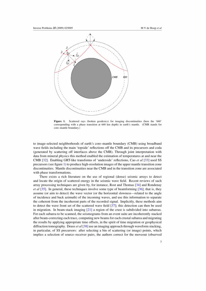
Figure 1. Scattered rays (broken geodesics) for imaging discontinuities (here the ‘660’corresponding with a phase transition at 660 km depth) in earth’s mantle. (CMB stands forcore–mantle boundary.)

to image-selected neighborhoods of earth’s core–mantle boundary (CMB) using broadbandwave fields including the main ‘topside’ reflections off the CMB and its precursors and coda(generated by scattering off interfaces above the CMB). Through joint interpretation withdata from mineral physics this method enabled the estimation of temperatures at and near theCMB [32]. Enabling GRT-like transforms of ‘underside’ reflections, Cao et al [33] used SSprecursors (see figure 1) to produce high-resolution images of the upper mantle transition zonediscontinuities. Mantle discontinuities near the CMB and in the transition zone are associatedwith phase transformations.

There exists a rich literature on the use of regional (dense) seismic arrays to detectand locate the origin of scattered energy in the seismic wave field. Recent reviews of sucharray processing techniques are given by, for instance, Rost and Thomas [34] and Rondenayet al [35]. In general, these techniques involve some type of beamforming [36]; that is, theyassume (or aim to detect) the wave vector (or the horizontal slowness—related to the angleof incidence and back azimuth) of the incoming waves, and use this information to separatethe coherent from the incoherent parts of the recorded signal. Implicitly, these methods aimto detect the wave front set of the scattered wave field [37]; this detection can then be usedin migration. In beam-stack imaging [21] a region of the crust is subdivided into subareas.For each subarea to be scanned, the seismograms from an event suite are incoherently stackedafter beam-correcting each trace, computing new beams for each crustal subarea and migratingthe results by applying appropriate time offsets, in the spirit of time migration or geophysicaldiffraction tomography. Deuss et al [38] use an imaging approach through waveform stacking,in particular, of SS precursors: after selecting a bin of scattering (or image) points, whichimplies a selection of source–receiver pairs, the authors correct for the moveout (observed

3

Inverse Problems 25 (2009) 025005 M V de Hoop et al

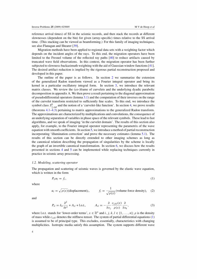
reference arrival times) of SS in the seismic records, and then stack the records at differentslownesses (dependent on the bin) for given (array-specific) times relative to the SS arrivaltime. (This stacking can be viewed as beamforming.) For this family of imaging techniques,see also Flanagan and Shearer [39].

Migration methods have been applied to regional data sets with a weighting factor whichdepends on the incident angles of the rays. To this end, the migration operators have beenlimited to the Fresnel volume of the reflected ray paths [40] to reduce artifacts caused bytruncated wave field observations. In this context, the migration operator has been furthersubjected to slowness-backazimuth weighting with the aid of Gaussian window functions [41].The desired artifact reduction is implied by the rigorous partial reconstruction proposed anddeveloped in this paper.

The outline of the paper is as follows. In section 2 we summarize the extensionof the generalized Radon transform viewed as a Fourier integral operator and bring itskernel in a particular oscillatory integral form. In section 3, we introduce the relevantmatrix classes. We review the (co-)frame of curvelets and the underlying dyadic parabolicdecomposition in appendix A. We then prove a result pertaining to the diagonal approximationof pseudodifferential operators (lemma 3.1) and the computation of their inverses on the rangeof the curvelet transform restricted to sufficiently fine scales. To this end, we introduce thesymbol class S0

12 ,rad

and the notion of a ‘curvelet-like function’. In section 4, we prove results

(theorems 4.1–4.3) pertaining to matrix approximations to the generalized Radon transform.The approximations are characterized by multiplications and convolutions, the consequence ofan underlying separation of variables in phase space of the relevant symbols. These lead to fastalgorithms, and we speak of imaging ‘in the curvelet domain’. The results of this section alsoapply, for example, to the Fourier integral operator representing the parametrix of the waveequation with smooth coefficients. In section 5, we introduce a method of partial reconstructionincorporating ‘illumination correction’ and prove the necessary estimates (lemma 5.1). Theresults of this section can be directly extended to other imaging schemes as long asthe canonical relation describing the propagation of singularities by the scheme is locallythe graph of an invertible canonical transformation. In section 6, we discuss how the resultspresented in sections 4 and 5 can be implemented while replacing techniques currently inpractice in seismic array processing.

1.2. Modeling, scattering operator

The propagation and scattering of seismic waves is governed by the elastic wave equation,which is written in the form

Pilul = fi, (1)

where

ul =√

ρ(x)(displacement)l, fi = 1√ρ(x)

(volume force density)i (2)

and

Pil = δil

∂2

∂t2+ Ail + l.o.t., Ail = − ∂

∂xj

cijkl(x)

ρ(x)

∂

∂xk

, (3)

where l.o.t. stands for ‘lower-order terms’, x ∈ Rn and i, j, k, l ∈ {1, . . . , n}; ρ is the density

of mass while cijkl denotes the stiffness tensor. The system of partial differential equations (1)is assumed to be of principal type. This excludes, essentially, characteristics with changingmultiplicities. Isotropic media satisfy this assumption. The system supports different wave

4

Inverse Problems 25 (2009) 025005 M V de Hoop et al

types (also called modes), one ‘compressional’ and n − 1 ‘shear’. We label the modes byM,N, . . . .

For waves in mode M, singularities are propagated along bicharacteristics, which aredetermined by Hamilton’s equations with Hamiltonian BM ; that is,

dx

dλ= ∂

∂ξBM(x, ξ),

dt

dλ= 1,

(4)dξ

dλ= − ∂

∂xBM(x, ξ),

dτ

dλ= 0.

The BM(x, ξ) follow from the diagonalization of the principal symbol matrix of Ail(x, ξ),namely as the (distinct) square roots of its eigenvalues. Clearly, the solution of (4) may beparameterized by t (that is, λ = t). We denote the solution of (4) with initial values (x0, ξ0) att = 0 by (xM(x0, ξ0, t), ξM(x0, ξ0, t)).

To introduce the scattering of waves, the total value of the medium parameters ρ, cijkl

is written as the sum of a smooth background component, ρ(x), cijkl(x), and a singularperturbation, δρ(x), δcijkl(x), namely ρ(x) + δρ(x), cijkl(x) + δcijkl(x). This decompositioninduces a perturbation of Pil (cf (3)),

δPil = δil

δρ(x)

ρ(x)

∂2

∂t2− ∂

∂xj

δcijkl(x)

ρ(x)

∂

∂xk

.

The scattered field, δul , in the single scattering approximation, satisfies

Pilδul = −δPilul.

Data are measurements of the scattered wave field, δu. When no confusion is possible,we denote data by u, however. We assume point sources (consistent with the far-fieldapproximation) and point receivers. Then the scattered wave field is expressible in termsof the Green’s function perturbations, δGMN(x, x, t), with incident modes of propagation Ngenerated at x and scattered modes of propagation M observed at x as a function of time. Here,(x, x, t) are contained in some acquisition manifold. This is made explicit by introducing thecoordinate transformation, y �→ (x(y), x(y), t (y)), such that y = (y ′, y ′′) and the acquisitionmanifold, Y say, is given by y ′′ = 0. We assume that the dimension of y ′′ is 2 + c, where c isthe codimension of the acquisition geometry. In this framework, the data are modeled by(

δρ(x)

ρ(x),δcijkl(x)

ρ(x)

)�→ δGMN(x(y ′, 0), x(y ′, 0), t (y ′, 0)). (5)

When no confusion is possible, we use the notation δGMN(y ′).We denote scattering points by x0; x0 ∈ X ⊂ R

n, reflecting that supp δρ ⊂ X andsupp δc ⊂ X. The bicharacteristics connecting the scattering point to a receiver (in mode M)or a source (in mode N) can be written as solutions of (4),

x = xM(x0, ξ0, t), x = xN(x0, ξ0, t ),

ξ = ξM(x0, ξ0, t ), ξ = ξN(x0, ξ0, t),

with appropriately chosen ‘initial’ ξ0 and ξ0, respectively. Then t = t + t representsthe ‘two-way’ reflection time. The frequency τ satisfies τ = −BM(x0, ξ0). We obtain(y(x0, ξ0, ξ0, t , t ), η(x0, ξ0, ξ0, t , t )) by transforming (x, x, t + t, ξ , ξ , τ ) to (y, η) coordinates.We then invoke the following assumptions that concern scattering over π and rays grazing theacquisition manifold.

Assumption 1. There are no elements (y ′, 0, η′, η′′) with (y ′, η′) ∈ T ∗Y\0 such that thereis a direct bicharacteristic from (x(y ′, 0), ξ (y ′, 0, η′, η′′)) to (x(y ′, 0),−ξ (y ′, 0, η′, η′′)) witharrival time t (y ′, 0).

5

Inverse Problems 25 (2009) 025005 M V de Hoop et al

Assumption 2. The matrix

∂y ′′

∂(x0, ξ0, ξ0, t , t )has maximal rank. (6)

With assumptions 1 and 2, equation (5) defines a Fourier integral operator of order n−1+c4

and canonical relation, that governs the propagation of singularities, given by

MN = {(y ′(x0, ξ0, ξ0, t , t ), η′(x0, ξ0, ξ0, t , t ); x0, ξ0 + ξ0)|

BM(x0, ξ0) = BN(x0, ξ0) = −τ, y ′′(x0, ξ0, ξ0, t , t ) = 0} (7)

⊂ T ∗Y\0 × T ∗X\0

[4, 9, 12]. The condition y ′′(x0, ξ0, ξ0, t , t ) = 0 determines the traveltimes t for given(x0, ξ0) and t for given (x0, ξ0). The canonical relation admits coordinates, (y ′

I , x0, η′J ),

where I ∪ J is a partition of {1, . . . , 2n − 1 − c}, and has an associated phase function,�MN = �MN(y ′, x0, η

′J ). While establishing a connection with double beamforming, we will

also use the notation xs = x(y ′, 0), xr = x(y ′, 0); when no confusion is possible, we use thesimplified notation y ′ = (xs, xr , t).

We refer to the operator above as the scattering operator. Its principal symbol can beexplicitly computed in terms of solutions of the transport equation [12]. In the further analysiswe suppress the subscripts MN, and drop the prime and write y for y ′ and η for η′.

2. Generalized Radon transform

Through an extension, the scattering operator becomes, microlocally, an invertible Fourierintegral operator, the canonical relation of which is a graph. The inverse operator acts onseismic reflection data and describes inverse scattering by the generalized Radon transform.

2.1. Extension

Subject to the restriction to the acquisition manifold Y, the data are a function of 2n − 1 − c

variables, while the singular part of the medium parameters is a function of n variables. Here,we discuss the extension of the scattering operator to act on distributions of 2n−1−c variables,equal to the number of degrees of freedom in the data acquisition. We recall the commonlyinvoked assumption as follows.

Assumption 3. (Guillemin [42]) The projection πY of on T ∗Y\0 is an embedding.

This assumption is known as the Bolker condition. It admits the presence of caustics.Because is a canonical relation that projects submersively on the subsurface variables (x, ξ)

(using that the matrix operator Pil is of principal type), the projection of (7) on T ∗Y\0 isimmersive [43, lemmas 25.3.6 and 25.3.4]. Indeed, only the injectivity part of the Bolkercondition needs to be verified. The image L of πY is locally a co-isotropic submanifold ofT ∗Y\0.

Since the projection πX of on T ∗X\0 is submersive, we can choose (x, ξ) as the first2n local coordinates on ; the remaining dim Y − n = n − 1 − c coordinates are denoted bye ∈ E,E being a manifold itself. Moreover, ν = ‖ξ‖−1ξ is identified as the seismic migrationdip. The sets X � (x, ξ) = const are the isotropic fibers of the fibration of Hormander [44],theorem 21.2.6; see also theorem 21.2.4. The wave front set of the data is contained in L andis a union of such fibers. The map πXπ−1

Y : L → X is a canonical isotropic fibration, whichcan be associated with seismic map migration [45].

6

Inverse Problems 25 (2009) 025005 M V de Hoop et al

With assumption 3 being satisfied, we define as the map (on ),

: (x, ξ, e) �→ (y(x, ξ, e), η(x, ξ, e)) : T ∗X\0 × E → T ∗Y\0;this map conserves the symplectic form of T ∗X\0. The (x, ξ, e) are ‘symplectic’ coordinateson the projection L of on T ∗Y\0. In the following lemma, these coordinates are extended tosymplectic coordinates on an open neighborhood of L, which is a manifestation of Darboux’stheorem stating that T ∗Y can be covered with symplectic local charts.

Lemma 2.1. Let L be an embedded co-isotropic submanifold of T ∗Y\0, with symplecticcoordinates (x, ξ, e). Denote L � (y, η) = (x, ξ, e). We can find a homogeneous canonicalmap G from an open part of T ∗(X × E)\0 to an open neighborhood of L in T ∗Y\0, such thatG(x, e, ξ, ε = 0) = (x, ξ, e).

Let M be the canonical relation defined as the graph of map G in this lemma, i.e.

M = {(G(x, e, ξ, ε); x, e, ξ, ε)} ⊂ T ∗Y\0 × T ∗(X × E)\0.

One can then construct a Maslov-type phase function for M that is directly related to a phasefunction for . Suppose (yI , x, ηJ ) are suitable coordinates for . For |ε| small, the constant-ε subset of M allows the same set of coordinates, thus we can use coordinates (yI , ηJ , x, ε) onM. Now there is (see theorem 4.21 in Maslov and Fedoriuk [46]) a function S(yI , x, ηJ , ε),called the generating function, such that M is given by

yJ = ∂S

∂ηJ

, ηI = − ∂S

∂yI

,

(8)ξ = ∂S

∂x, e = −∂S

∂ε.

A phase function for M is hence given by

�(y, x, e, ηJ , ε) = S(yI , x, ηJ , ε) − 〈ηJ , yJ 〉 + 〈ε, e〉. (9)

A phase function for is then recovered by

�

(y, x,

∂S

∂ε

∣∣∣∣ε=0

, ηJ , 0

)= �(y, x0, ηJ ).

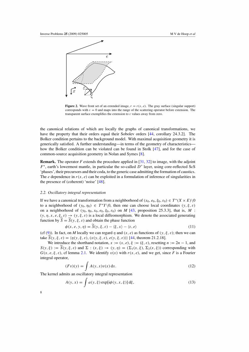
We then obtain a mapping from a reflectivity function (illustrated in figure 2) to reflectiondata that extends the mapping from contrast to data (cf (5)). We recall the following theorem.

Theorem 2.2. [12] Suppose microlocally that assumptions 1 (no scattering over π ), 2(transversality), and 3 (Bolker condition) are satisfied. Let F be the Fourier integral operator,

F : E ′(X × E) → D′(Y ),

with canonical relation given by the graph of the extended map G : (x, ξ, e, ε) �→ (y, η)

constructed in lemma 2.1. Then the data can be modeled by F acting on a distribution r(x, e)

of the form

r(x, e) = R(x,Dx, e)c(x), (10)

where R stands for a smooth e-family of pseudodifferential operators and c ∈ E ′(X) withc = ( δcijkl

ρ,

δρ

ρ

).

The operator F is microlocally invertible. By composing with an elliptic pseudodifferentialoperator we can assume without loss of generality that F is a zeroth-order Fourier integraloperator associated with a (local) canonical graph. We recall that for Fourier integral operators

7

Inverse Problems 25 (2009) 025005 M V de Hoop et al

Figure 2. Wave front set of an extended image, r = r(x, e). The gray surface (singular support)corresponds with ε = 0 and maps into the range of the scattering operator before extension. Thetransparent surface exemplifies the extension to ε values away from zero.

the canonical relations of which are locally the graphs of canonical transformations, wehave the property that their orders equal their Sobolev orders [44, corollary 24.3.2]. TheBolker condition pertains to the background model. With maximal acquisition geometry it isgenerically satisfied. A further understanding—in terms of the geometry of characteristics—how the Bolker condition can be violated can be found in Stolk [47], and for the case ofcommon-source acquisition geometry in Nolan and Symes [8].

Remark. The operator F extends the procedure applied in [31, 32] to image, with the adjointF ∗, earth’s lowermost mantle, in particular the so-called D′′ layer, using core-reflected ScS‘phases’, their precursors and their coda, to the generic case admitting the formation of caustics.The e dependence in r(x, e) can be exploited in a formulation of inference of singularities inthe presence of (coherent) ‘noise’ [48].

2.2. Oscillatory integral representation

If we have a canonical transformation from a neighborhood of (x0, e0, ξ0, ε0) ∈ T ∗(X ×E)\0to a neighborhood of (y0, η0) ∈ T ∗Y\0, then one can choose local coordinates (y, ξ, ε)

on a neighborhood of (y0, η0, x0, e0, ξ0, ε0) on M [43, proposition 25.3.3], that is, M :(y, η, x, e, ξ, ε) → (y, ξ, ε) is a local diffeomorphism. We denote the associated generatingfunction by S = S(y, ξ, ε) and obtain the phase function

φ(x, e, y, η) = S(y, ξ, ε) − 〈ξ, x〉 − 〈ε, e〉 (11)

(cf (9)). In fact, on M locally we can regard η and (x, e) as functions of (y, ξ, ε); then we cantake S(y, ξ, ε) = 〈η(y, ξ, ε), (x(y, ξ, ε), e(y, ξ, ε))〉 [44, theorem 21.2.18].

We introduce the shorthand notation, x := (x, e), ξ := (ξ, ε), resetting n := 2n − 1, andS(y, ξ) := S(y, ξ, ε) and � : (x, ξ) → (y, η) = (�1(x, ξ),�2(x, ξ)) corresponding withG(x, e, ξ, ε), cf lemma 2.1. We identify v(x) with r(x, e), and we get, since F is a Fourierintegral operator,

(Fv)(y) =∫

A(y, x)v(x) dx. (12)

The kernel admits an oscillatory integral representation

A(y, x) =∫

a(y, ξ) exp[iφ(y, x, ξ)] dξ, (13)

8

Inverse Problems 25 (2009) 025005 M V de Hoop et al

with non-degenerate phase function

φ(y, x, ξ) = S(y, ξ) − 〈ξ, x〉 (14)

and amplitude a = a(y, ξ), a standard symbol of order zero, with principal part homogeneousin ξ of order 0. With the above form of the phase function, it follows immediately that operatorF propagates singularities according to the map,(

∂S

∂ξ, ξ

)→

(y,

∂S

∂y

), (15)

which can be identified as �. Substituting (14) into (12) and (13) yields the representation

(Fv)(y) =∫

a(y, ξ) exp[iS(y, ξ)]v(ξ) dξ, (16)

in which S satisfies the homogeneity property S(y, cξ) = cS(y, ξ) for c > 0; v denotes theFourier transform of v, and dξ denotes (2π)−n times the Lebesgue measure.

We remark that the above representation is valid microlocally. In section 4 we studythe action of operators of the form (16) to curvelets. The results for the global Fourierintegral operator F are obtained by taking a superposition of the above representations usingan appropriate microlocal partition of the unity in phase space.

3. Matrix classes and operator approximations

3.1. ‘Curvelets’, matrix classes and operators

The (co)frame of curvelets, ϕγ , ψγ , is defined in (A.3). We introduce the notation C for thecurvelet transform (analysis): vγ = (Cv)γ (cf (A.4)), and also define C−1{cγ } = ∑

γ cγ ϕγ forthe inverse transform (synthesis). We observe that C−1 C = I on L2(Rn), and that CC−1 ≡ �

is a (not necessarily orthogonal) projection operator of �2γ onto the range of the analysis

operator C. It holds that �2 = �, but � is generally not self-adjoint unless ψγ = ϕγ .Observe that, as a matrix on �2

γ ,

�γ ′γ = 〈ψγ ′ , ϕγ 〉.If A : L2(Rn) → L2(Rn), then the matrix [A] = CA C−1 preserves the range of C, sinceC−1� = C−1, and �C = C. In particular, [A]� = �[A] = [A]. Here, and when convenient,we identify operators on �2

γ with matrices.Let d denote the pseudodistance on S∗(X) introduced in [49, definition 2.1]

d(x, ν; x ′, ν ′) = |〈ν, x − x ′〉| + |〈ν ′, x − x ′〉|+ min{‖x − x ′‖, ‖x − x ′‖2} + ‖ν − ν ′‖2.

If γ = (x, ν, k) and γ ′ = (x ′, ν ′, k′), let

d(γ ; γ ′) = 2− min(k,k′) + d(x, ν; x ′, ν ′). (17)

The weight function μδ(γ, γ ′) introduced in [50] is given by

μδ(γ, γ ′) = (1 + |k′ − k|2)−12−( 12 n+δ)|k′−k|2−(n+δ) min(k′,k)d(γ, γ ′)−(n+δ).

We summarize [50, definitions 2.6–2.8]. If χ is a mapping on S∗(Rn), the matrix M withelements Mγ ′γ belongs to the class Mr

δ(χ), if there is a constant C(δ) such that

|Mγ ′γ | � C(δ)2krμδ(γ′, χ(γ )) (2kr ≈ ‖ξ‖r ); (18)

here, χ(γ ) = (χ(xj , ν), k). Furthermore, Mr (χ) = ∩δ>0Mrδ(χ). If χ is the projection

of a homogeneous canonical transformation, then by [49, lemma 2.2] the map χ preserves

9

Inverse Problems 25 (2009) 025005 M V de Hoop et al

the distance d up to a bounded constant; that is d(χ−1(γ ), γ ′) ≈ d(γ, χ(γ ′)). Hence, thetranspose operation takes matrices in Mr (χ) to Mr (χ−1). We note that the projection map� = CC−1 belongs to M0(I ), see [50, lemma 2.9].

It is also useful to introduce norms on the class of matrices determined by distance-weighted �2

γ norms on columns and rows. Precisely, for α � 0 and a given χ ,

‖M‖22;α = sup

γ

∑γ ′

22|k−k′|α22 min(k,k′)αd(γ ′;χ(γ ))2α|Mγ ′γ |2

+ supγ ′

∑γ

22|k−k′|α22 min(k,k′)αd(γ ′;χ(γ ))2α|Mγ ′γ |2. (19)

We remark that any matrix bounded on �2γ must have finite (2; 0) norm, since this corresponds

to rows and columns being square summable. Additionally, it follows immediately that

‖M‖2;α+n < ∞ ⇒ M ∈ M0α(χ). (20)

Inclusion in the other direction follows from the proof of [50, lemma 2.4]

M ∈ M0α(χ) ⇒ ‖M‖2;α < ∞. (21)

The technique of (2;α) bounds has been designed for propagation and scattering problemsin rough background metrics (density normalized stiffness), but the Mr

δ conditions lead moredirectly to desired mapping properties.

3.2. Pseudodifferential operators and diagonal approximation

Pseudodifferential operators, of order r, with appropriate symbols are the most importantexample of operators with matrices of class Mr (I ).

Let

Av(x) ≡ a(x,D)v(x) =∫

exp[i〈x, ξ 〉]a(x, ξ )u(ξ) dξ,

where the symbol satisfies, for all j, α, β,∣∣〈ξ, ∂ξ 〉j ∂αξ ∂β

x a(x, ξ)∣∣ � Cj,α,β(1 + ‖ξ‖)− 1

2 |α|+ 12 |β|. (22)

We denote the class of symbols satisfying these estimates as S012 ,rad

. Thus, a ∈ S012 ,rad

precisely

when 〈ξ, ∂ξ 〉j a ∈ S012 , 1

2for all j . More generally, a ∈ Sr

12 ,rad

precisely when 〈ξ, ∂ξ 〉j a ∈ Sr12 , 1

2

for all j . Let A be a pseudodifferential operator with symbol in Sr12 ,rad

. A stationary phase

analysis then shows that Aϕγ = 2krfγ , where

fγ (ξ) = ρ−1/2k gν,k(ξ) exp[−i〈xj , ξ 〉], (23)

in which gν,k satisfies the estimates

|〈ν, ∂ξ 〉j ∂αξ gν,k| � Cj,α,N 2−k(j+ 1

2 |α|)(1 + 2−k|〈ν, ξ 〉| + 2−k/2‖ξ − Bν,k‖)−N

for all N, where ‖ξ − Bν,k‖ denotes the distance of ξ to the rectangle Bν,k supporting χν,k .Such an fγ will be called a ‘curvelet-like function’ centered at γ , cf (A.3). In particular,

|〈ψγ ′ , fγ 〉| � C(δ)μδ(γ′, γ )

for all δ > 0, so that 〈ψγ ′ , fγ 〉 ∈ M0(I ).If the principal symbol of A is homogeneous of order 0, a0(x, ξ) = a0(x, ξ/‖ξ‖), we have

the following diagonalization result, which is a simple variation of the phase-linearization ofSeeger–Sogge–Stein [52].

10

Inverse Problems 25 (2009) 025005 M V de Hoop et al

Lemma 3.1. Suppose that A is a pseudodifferential operator with homogeneous principlesymbol a0(x, ξ) of order 0. Then

Aϕγ = a0(xj , ν)ϕγ + 2−k/2fγ , (24)

where fγ is a curvelet-like function centered at γ .

Proof. The precise assumption we need is that the symbol of A equals a0 plus a symbol of

class S− 1

212 ,rad

. The terms of order − 12 can be absorbed into fγ , while

a0(x,D)ϕγ (x) = ρ−1/2k

∫exp[i〈x − xj , ξ 〉]a0(x, ξ)χν,k(ξ) dξ.

For convenience we assume that ν = (1, 0, . . . , 0) lies on the ξ1 axis. By homogeneity,a0(x, ξ) = a0(x, 1, ξ ′′/ξ1), where ξ ′′ = (ξ2, . . . , ξn). We take the first-order Taylor expansionon a cone about the ξ1 axis, that is,

a0(x, 1, ξ ′′/ξ1) − a0(xj , ν) = b1(x, ξ) · (x − xj ) + b2(x, ξ) · ξ ′′/ξ1,

where b1 and b2 are smooth homogeneous symbols. The term with ξ ′′/ξ1 is bounded by 2−k/2

on the support of χν,k , and preserves the derivative bounds (23) on χν,k with a gain of 2−k/2.The term b1 · (x − xj ) leads to a contribution

ρ−1/2k

∫exp[i〈x − xj , ξ 〉]Dξ(b1(x, ξ)χν,k(ξ)) dξ,

which also yields a curvelet-like function of order − 12 . �

In (24) we write rγ = 2−k/2fγ . Taking inner products with ψγ ′ yields

[A]γ ′γ = a0(xj , ν)�γ ′γ + 〈ψγ ′ , rγ 〉. (25)

If A is elliptic, we have uniform upper and lower bounds on the symbol a0(x, ξ), that isC−1 � |a0(x, ξ)| � C for some positive constant C. By (25) we then have

a0(xj , ν)−1[A]γ ′γ − �γ ′γ ∈ M− 12 (I ). (26)

Also, by (25),

|a0(xj , ν) − 〈ψγ , ϕγ 〉−1[A]γ γ | � C2−k/2.

It follows that (26) holds with a0(xj , ν) replaced by the normalized diagonal

Dγ = �−1γ γ [A]γ γ ,

after modifying [A]γ γ , if necessary, by terms of size 2−k/2, to allow for the possibility that thediagonal elements of [A] may vanish for small k.

We remark that (26) also holds with a0(xj , ν) replaced by a0(x′j , ν

′). (The latter appearsfrom applying the procedure of diagonal approximation to the adjoint of A.) This follows by(25) and the fact that

|a0(xj , ν) − a0(x′j , ν

′)| � C(|xj − x ′j | + |ν − ν ′|) � Cd(xj , ν; x ′

j , ν′)1/2,

hence the commutator (a0(x′j , ν

′) − a0(xj , ν))�γ ′γ belongs to M− 12 (I ). As above, it then

follows that

D−1γ ′ [A]γ ′γ = �γ ′γ + Rγ ′γ , R ∈ M− 1

2 (I ). (27)

While A need not be invertible, (27) implies that one can invert [A] on the range of Crestricted to k sufficiently large. Precisely, let �0 be a collection of indices γ . We denote by 1�0

the multiplication operator (diagonal) on �2γ that truncates a sequence to �0. Then ��0 = �1�0

11

Inverse Problems 25 (2009) 025005 M V de Hoop et al

is an approximate projection into the range of C, with rapidly decreasing coefficients awayfrom �0. In practice, it is desirous to take 1�0 , at each fixed scale k, to be a smooth truncationto a neighborhood of �0, such that

∣∣1�0γ − 1

�0γ ′

∣∣ � Cd(γ, γ ′)1/2. In this case,(1�0

γ − 1�0γ ′

)�γγ ′ ∈ M− 1

2 , (28)

so that 1�0 preserves the range of C at any fixed scale k up to an operator of norm 2−k/2, hencethe difference between ��0 and 1�0 is small on the range of C for large k.

If we multiply (27) on the right by 1�0γ , and use that R = R�, then

D−1[A]1�0 = �1�0 + R1�0 = (I + R0)��0 ,

where R0 is the matrix R restricted to the scales k occurring in �0. Hence, if �0 is supportedby k sufficiently large, then I + R0 can be inverted, and

(I + R0)−1D−1[A]1�0 = ��0 ,

using a Neumann expansion. To leading order the inverse is diagonal. We will exploit thisresult in section 5, while solving the normal equations derived from the composition F ∗F ,yielding ‘illumination correction’ and partial reconstruction of the reflectivity function.

4. Generalized Radon transform matrix approximation

We consider the action of the generalized Radon transform operator F on a single curvelet,that is v = ϕγ in (16),

(Fϕγ )(y) = ρ−1/2k

∫a(y, ξ)χν,k(ξ) exp[i(S(y, ξ) − 〈ξ, xj 〉)] dξ. (29)

With the outcome, we can associate a ‘kernel’

Aν,k(y, xj ) = (Fϕγ )(y). (30)

The infinite generalized Radon transform matrix is given by

[F ]γ ′γ :=∫

ψγ ′(y)(Fϕγ )(y) dy =∫

ψγ ′(y)Aν,k(y, xj ) dy. (31)

We then have F = C−1[F ]C.We seek an approximation of Fϕγ via expansions of the generating function S(y, ξ) and

the symbol a(y, ξ) near the microlocal support of ϕγ . The first-order Taylor expansion ofS(y, ξ) along the ν-axis, following [52], yields

S(y, ξ) − 〈ξ, xj 〉 =⟨ξ,

∂S

∂ξ(y, ν) − xj

⟩+ h2(y, ξ), (32)

where the error term h2(y, ξ) satisfies the estimates (22) on the ξ -support of χν,k .Consequently, exp[ih2(y, ξ)] is a symbol of class S0

12 ,rad

if ξ is localized to the rectangle

Bν,k supporting χν,k .We introduce the coordinate transformation (note that ν depends on k)

y → Tν,k(y) = ∂S

∂ξ(y, ν).

If bν,k(x, ξ) is the order 0 symbol

bν,k(x, ξ) = (a(y, ξ) exp[ih2(y, ξ)])|y=T −1ν,k (x),

then

(Fϕγ )(y) = [bν,k(x,D)ϕγ ]x=Tν,k(y).

12

Inverse Problems 25 (2009) 025005 M V de Hoop et al

This decomposition expresses the generalized Radon transform operator as a (ν, k)-dependentpseudodifferential operator followed by a change of coordinates, also depending on the pair(ν, k). This decomposition can be used to show that the matrix [F ] belongs to M0(χ), whereχ is the projection of the homogeneous canonical transformation � (cf (15)) to the co-spherebundle. (See also theorem 4.3.)

We use an expansion of the symbol and phase of the oscillatory integral representation toobtain an approximation for the generalized Radon transform matrix elements up to an errorof size 2−k/2; more precisely, the matrix errors will be of class M− 1

2 (χ). The principal parta0(y, ξ) of symbol a(y, ξ) is homogeneous of order 0. Following lemma 3.1, we may replacea0(y, ξ) by either a0(y, ν) or a0(yj , ν), where

xj = ∂S

∂ξ(yj , ν) = Tν,k(yj ),

with the effect of modifying the generalized Radon transform matrix by a matrix of classM− 1

2 (χ).The symbol h2(y, ξ) is homogeneous of order 1 and of class S0

12 ,rad

on the support of

χν,k , whence we need account for the second-order terms in its Taylor expansion to obtainan approximation within order − 1

2 . The relevant approximation is to Taylor expand in ξ

in directions perpendicular to ν, preserving homogeneity of order 1 in the radial direction;this is dictated by the non-isotropic geometry of the second-dyadic (or dyadic parabolic)decomposition.

For convenience of notation, we consider the case that ν lies on the ξ1 axis. Then (compare(32))

S(y, ξ1, ξ′′) = ξ1S(y, 1, ξ ′′/ξ1) = ξ · ∂S

∂ξ(y, ν) +

1

2

ξ ′′2

ξ1· ∂2S

∂ξ ′′2 (y, ν) + h3(y, ξ),

where h3(y, ξ) ∈ S− 1

212 ,rad

if ξ is restricted to the support of χν,k . Replacing the symbol

exp[ih3(y, ξ)] by 1 changes the matrix by terms of class M− 12 (χ), as in the proof of

lemma 3.1. Consequently, up to errors of order − 12 , one can replace the symbol

a(y, ξ) exp[ih2(y, ξ)] on Bν,k by

a(y, ν) exp[i 1

2ξ−11 ξ ′′2 · ∂2

ξ ′′S(y, ν)]1Bν,k

(ξ)

with 1Bν,ka smooth cutoff to the rectangle Bν,k supporting χν,k .

The exponent separates the variables y and ξ , and is bounded by a constant, independent of(ν, k). Approximating the complex exponential for bounded (by C) arguments by a polynomialfunction leads to a tensor-product representation of the symbol

a(y, ν) exp

[i1

2ξ−1

1 ξ ′′2 · ∂2ξ ′′S(y, ν)

]≈

N∑s=1

α1s;ν,k(y)α2

s;ν,k(ξ).

To obtain an error of size 2−k/2 requires CN/N! � 2−k/2, or N ∼ k/ log k.

Theorem 4.1. With N ∼ k/ log k, one may express

(Fϕγ )(y) =N∑

s=1

α1s;ν,k(y)

(α2

s;ν,k ∗ ϕγ

) ◦ Tν,k(y) + 2−k/2fγ , (33)

where fγ is a curvelet-like function centered at χ(γ ).

An alternative approximation starts with replacing a(y, ξ) or a(y, ν) by a(yj , ν) withyj = T −1

ν,k (xj ) (and γ = (xj , ν, k)). Similarly, up to an error of order − 12 , one may replace

13

Inverse Problems 25 (2009) 025005 M V de Hoop et al

ξ−11 ξ ′′2 · ∂2

ξ ′′S(y, ν) by ξ−11 ξ ′′2 · ∂2

ξ ′′S(yj , ν). Consequently, replacing bν,k(x, ξ) by the x-independent symbol

bγ (ξ) = a(yj , ν) exp[i 1

2ξ−11 ξ ′′2 · ∂2

ξ ′′S(yj , ν)]1Bν,k

(ξ) = αγ (ξ),

modifies the generalized Radon transform matrix by terms in M− 12 (χ). Precisely,

Theorem 4.2. One may express

(Fϕγ )(y) = (αγ ∗ ϕγ ) ◦ Tν,k(y) + 2−k/2fγ (34)

where fγ is a curvelet-like function centered at χ(γ ).

This is a generalization of the geometrical, zeroth-order approximation of the common-offset realization—valid in the absence of caustics—of the generalized Radon transformconsidered in [53]. In theorem 4.2, as well as theorem 4.3, the terms in the approximationare determined by the geometry of the underlying canonical transformation (ray tracing). Anapproach based upon uniform approximation of the symbol and zeroth-order phase terms byfunctions which separate space and frequency variables, as in theorem 4.1, was studied ingreater depth in [55].

The change of variables Tν,k can also be suitably approximated by a local expansionof the generating function about (yj , ν). This requires an approximation of the phase⟨ξ, ∂S

∂ξ(y, ν) − xj

⟩up to an error of size 2−k/2 (cf (32)), which is accomplished by taking

the second-order expansion in y about yj . Precisely, we write

∂S

∂ξ(y, ν) − xj = ∂2S

∂ξ∂y(yj , ν) · (y − yj ) +

1

2

∂3S

∂ξ∂y2(yj , ν) · (y − yj )

2 + h3(y, ν), (35)

where h3(y, ν) vanishes to third order at y = yj , and hence ξ · h3(y, ν) leads to terms oforder 2−k/2 as in lemma 3.1. The first two terms on the right-hand side of (35) are exactly thequadratic expansion of Tν,k about y = yj .

In the expression ξ · ∂3S∂ξ∂y2 (yj , ν) · (y − yj )

2, the terms in ξ perpendicular to ν are of size

2k/2 as opposed to 2k for the component of ξ parallel to ν, hence lead to terms of size 2−k/2.This allows one to replace the third-order derivative term by the quadratic expression

1

2

[ν · ∂3S

∂ξ∂y2(yj , ν) · (y − yj )

2

]ν

= 1

2

[∂2S

∂y2(yj , ν) · (y − yj )

2

]ν = Qγ · (y − yj )

2 (36)

with yj = T −1ν,k (xj ) (and γ = (xj , ν, k)) as before.

Theorem 4.3. One may express

(Fϕγ )(y) = (αγ ∗ ϕν,k) ◦ [DTγ · (y − yj ) + Qγ · (y − yj )2] + 2−k/2fγ , (37)

where fγ is a curvelet-like function centered at χ(γ ).

Here, the affine map DTγ = ∂Tν,k

∂y(yj ) = ∂2S

∂ξ∂y(yj , ν) can be decomposed into a rigid

motion and a shear. The shear factor acts in a bounded manner on the curvelet, in that itpreserves the position and direction; see also [51, 53].

The contribution Qγ · (y − yj )2 captures the curvature of the underlying canonical

transformation applied to the infinitesimal plane wave attached to ϕγ . As with the shearterm it acts in a bounded manner on a curvelet, and can be neglected in a zeroth-orderapproximation. This is the case in [50], where rigid approximations to Tν,k were taken. Both

14

Inverse Problems 25 (2009) 025005 M V de Hoop et al

shear and curvature terms must be accounted for to obtain an approximation up to errors ofsize 2−k/2.

The expansion in theorem 4.3 is analogous to the Gaussian beam expansion for isotropicwave packets evolving under the wave equation, that is, if F were the forward parametrix ofthe wave equation. A Gaussian beam is frequency localized to a ball of diameter 2k/2 in ξ ,and in the Gaussian beam expansion one considers quadratic expansions in ξ about the centerξ0 of the packet. For curvelets, the support is of dimension 2k in radial directions, and theapproximations to the phase must preserve homogeneity in the radial variable.

Remark. The matrix [F ∗], essentially, provides the means to perform generalized Radontransform imaging entirely in the curvelet domain (that is, ‘after double beamforming’).In this context, ‘beam-stack migration’ can be understood as ‘scanning’ the magnitude of〈Fδx0 , u〉 = ∑

γ 〈δx0 , F∗ϕγ 〉uγ = ∑

γ F ∗ϕγ (x0)uγ as a function of x0.

5. Partial reconstruction

In applications, the image will admit a sparse decomposition into curvelets. Suppose thegoal is to reconstruct the image contribution composed of a small set of curvelets (a ‘target’).The aim is to reconstruct this contribution by the available acquisition of data with the least‘artifacts’ (hence curvelets).

Let v denote a model of reflectivity, as before, and w its image, interrelated throughw = F ∗Fv. We write

N = F ∗F,

so that [N ] = [F ∗][F ]. The operator N is a pseudodifferential operator with polyhomogeneoussymbol of order 0; in particular, N has homogeneous principal symbol of order 0, and theresults of section 3.2 apply to N.

We describe a target region by the set of indices �0. Our resolution-illumination analysis isthus focused on the product [N ]��0 . The acquisition of data is accounted for by �S = �1S ,where S stands for the (finite) set of curvelets that can be observed given the acquisitiongeometry. The resolution is thus described by the operator, and matrix,

N = F ∗C−11S CF, [N] = [F ∗]1S [F ] = [F ∗]�S[F ], (38)

and the normal equation to be solved, yielding the partial reconstruction, is given by[N ]Cv = [F ∗]�S Cu, where �S Cu represents the observed data. The set S is assumedto contain a suitable neighborhood of χ(�0), in that d(γ, χ(γ0)) � 2−k for γ ∈ Sc andγ0 ∈ �0 at scale k. (Otherwise, �0, or S, need to be adjusted.) The matrix [N ] thenapproximates the matrix [N ] near �0 in the following sense.

Lemma 5.1. Let

��0 = infγ∈Sc,γ0∈�0

2|k0−k|2min(k0,k)d(γ ;χ(γ0)).

Then for all α, and m arbitrarily large, there exists a constant Cα,m such that

‖([N ] − [N ])��0‖2;α � Cα,m�−m�0

.

Proof. Since [F ∗]� = [F ∗] and [F ]� = [F ], the matrix [N ]��0 − [N]��0 takes the form∑γ ′′

[F ∗]γ γ ′′1Sc

γ ′′ [F ]γ ′′γ ′1�0γ ′ .

15

Inverse Problems 25 (2009) 025005 M V de Hoop et al

The sum is dominated by

Cδ,m

∑γ ′′

μδ(χ(γ ), γ ′′)1Sc

γ ′′μδ+m(γ ′′, χ(γ ′))1�0γ ′ .

We use the bound μδ+m(γ ′′, χ(γ ′)) � �−m�0

μδ(γ′′, χ(γ ′)) and [50, lemma 2.5], together with

invariance of the distance under χ , to bound the sum by Cδ,m�−m�0

μδ(γ, γ ′). The resultfollows, since ‖μδ(., .)‖2,α � 1 if δ � α. �

Finally, we explore the invertibility of [N ] on the range of ��0 . To this end, we introducean intermediate index set �1 with �0 ⊂ �1 ⊂ χ−1(S), for which ��1 ≈ ��0 , and with

‖��1��0 − ��0‖2;α � �−m�0

(39)

for m arbitrarily large. For γ in a set containing �1, then |[N]γ γ − [N ]γ γ | � 1. We introducethe inverse diagonal,

D−1γ = �γγ [N]−1

γ γ (40)

for γ near �1, and smoothly truncate D−1γ to 0 away from �1. Then

D−1[N ]��1 = ��1 + R,

where ‖R‖2,α � 1 if ��0 is sufficiently large, depending on the given α.If ��1 were a true projection then we would have R = R��1 , and applying (I + R)−1

would yield the desired inverse of [N ] on the range of ��1 . In the case of the approximateprojections ��0 ,��1 , one can obtain an approximate inverse against ��0 . We write

(I + R)−1D−1[N ]��1��0 = ��0 + (I + R)−1(��1��0 − ��0).

By (39) this yields

(I + R)−1D−1[N ]��0 = ��0 + R,

where ‖R‖2,α � 1, provided ��0 is sufficiently large, depending on the given α. Thus,by applying (I + R)−1D−1 to [F ∗]�S Cu, we obtain the desired, approximate, partialreconstruction of the reflectivity function, where C has replaced the notion of doublebeamforming, and [F ] and [F ∗] can now be replaced by their approximations developedin the previous section.

Remark. In practical applications, R and R are neglected. In general, with limitedillumination, the diagonal elements [N ]γ γ have to be estimated numerically through‘demigration’ followed by ‘remigration’ against ��0 . In the case of full illumination, thediagonal elements can be directly approximated using (25). For an optimization approach tosolving the normal equation, in this context, see Symes [56] and Herrmann et al [57].

Remark. The image of a single data curvelet is naturally given by w = F ∗ϕγ =∑γ ′[F ∗]γ ′γ ϕγ ′ whence wγ ′ = [F ∗]γ ′γ . From the fact that the matrix [F ∗] belongs to

M0(χ−1), it is immediate that for α arbitrarily large (cf (19))∑γ

22|k−k′|α22 min(k,k′)αd(γ ′;χ−1(γ ))2α|[F ∗]γ ′γ |2 � C

illustrating that the curvelet decomposition of the data eliminates the ‘isochrone smear’associated with imaging individual data samples.

16

Inverse Problems 25 (2009) 025005 M V de Hoop et al

6. Discussion

The results presented in this paper essentially provide a novel approach to imaging, based onthe generalized Radon transform, replacing the notions of ‘plane-wave migration’ and ‘beam-stack imaging’ by matrix approximations using curvelets on the one hand, and addressingthe problem of partial reconstruction on the other hand. However, the results presented insection 3.2 apply to general, elliptic, pseudodifferential operators, while the results presentedin section 4 pertain to all Fourier integral operators (of order zero) the canonical relation ofwhich is (locally) a canonical graph.

Application of the results presented in this paper, in the context of seismic array processing,consists of data decomposition into curvelets, imaging and reconstruction. We briefly discusseach step.

6.1. Decomposition

The curvelet transform applied to the data replaces the notion of double beamforming [36], atool used in seismic array processing [34]. Double beamforming can be introduced as follows.Let g be a real, even Schwartz function in R

n with ‖g‖L2 = (2π)−n/2; suppose that g issupported in the unit ball. For λ � 1, define

gλ(x; x0, ξ0) = λ−n/4 exp(i〈η, x − x0〉)g(λ1/2(x − x0)). (41)

The FBI transform [58] of u is then given by

U(x0, ξ0) = Tλu(x0, ξ0) =∫

u(x)gλ(x; x0, ξ0) dx. (42)

The adjoint, T ∗λ , of Tλ follows as

T ∗λ U(x) =

∫U(x0, ξ0)gλ(x; x0, ξ0) dx0 dξ0. (43)

We have the property T ∗λ Tλ = I .

For application to the data (see subsection 1.2), we identify y = (xs, xr , t) (replacing x)and η0 = τ(πs, πr , 1) (replacing ξ0). In the context and terminology of double beamforming,πs,r represent the slowness vectors. The remaining normal components of the associatedcovectors can be obtained by using that their norms equal the reciprocal wave speeds at x

s,r0 .

In the above, xr0 coincides typically with the geometrical center of the receiver array. It has

been noted that the applicability of beamforming requires relatively narrow-aperture arrays.To use earthquakes for source-array processing, normalizations have to be applied accountingfor source mechanisms and depths. Normalizations can be implemented as deconvolutions intime for each event. Furthermore, xs

0 in the above would be the location of a master event.Double beamforming is obtained as (changing order of integration4)

(Bu)(y0, πs, πr) = 1

2π

∫(Tλ=1u)(y0, τ (πs, πr , 1)) dτ. (44)

(Typically, one subjects the data, u, to rotations to separate the polarizations and identify aseismic phase prior to applying double beamforming.) Double beamforming aims to estimatethe variables (t0, π

s, πr), that is,(y0, π

s0 , πr

0

)for events (singularities) in the data [18].

In our procedure, Tλ is replaced by the curvelet transform, C, while the integration overτ is no longer carried out. One can think of setting λ = 2k and identifying in (42) x0 withxj and ξ0 with 2kν, and U(x0, ξ0) with uγ . In [59] discrete, almost symmetric wave packets

4 If g were replaced by a Gaussian function, Tλ=1 would be identified with the Gabor transform.

17

Inverse Problems 25 (2009) 025005 M V de Hoop et al

and a higher dimensional curvelet transform, acting on unevenly sampled data, have beendeveloped. To find a sparse decomposition, one can follow an �1 optimization procedure [60];we arrive at the index set S.

6.2. Imaging

Imaging structure in the earth with seismic array data has been carried out through first-orderTaylor expansions in xr (and xs) of the traveltime function (appearing in the canonical relation) about xr

0 (and xs0, with corresponding traveltime t0) relative to a prescribed scattering point

(x0 in (7)) defining slowness vectors; in the process, the amplitude (or semblance) of theoutcome using these traveltime-derived slowness vectors is displayed on a grid of scatteringpoints.

Here, we apply theorem 4.2, or 4.1, to generate an image from the decomposed data,which requires dynamical ray-tracing computations. The image is decomposed into curveletsyielding coefficients pertaining to the index set �1.

6.3. Reconstruction

For each index γ in the set �1, the diagonal entry [N]γ γ is computed. This is moststraightforwardly done by methods of so-called demigration–remigration, that is, following(38). One can apply the right-hand sides of (38) to the image obtained in the preceding step,and estimate a diagonal matrix acting on the curvelet-transformed image that recovers theresult. One then evaluates the inverse diagonal matrix (cf (40)) and applies the result to theoutcome of the imaging step to obtain the reconstruction (solution to the normal equations)on the index set �0.

Acknowledgment

The authors would like to thank A Deuss for stimulating discussions on beamforming.

Appendix A. Dyadic parabolic decomposition and ‘curvelet’

We introduce boxes (along the ξ1-axis, that is, ξ ′ = ξ1)

Bk =[ξ ′k − L′

k

2, ξ ′

k +L′

k

2

]×

[−L′′

k

2,L′′

k

2

]n−1

,

where the centers ξ ′k , as well as the side lengths L′

k and L′′k , satisfy the parabolic scaling

condition

ξ ′k ∼ 2k, L′

k ∼ 2k, L′′k ∼ 2k/2, as k → ∞.

Next, for each k � 1, let ν vary over a set of approximately 2k(n−1)/2 uniformly distributedunit vectors. (We can index ν by � = 0, . . . , Nk − 1, Nk ≈ �2k(n−1)/2�: ν = ν(�) while weadhere to the convention that ν(0) = e1 aligns with the ξ1-axis.) Let �ν,k denote a choice ofrotation matrix which maps ν to e1, and

Bν,k = �−1ν,kBk.

In the (co-)frame construction, we have two sequences of smooth functions, χν,k and βν,k , onR

n, each supported in Bν,k , so that they form a co-partition of unity

χ0(ξ)β0(ξ) +∑k�1

∑ν

χν,k(ξ)βν,k(ξ) = 1, (A.1)

18

Inverse Problems 25 (2009) 025005 M V de Hoop et al

and satisfy the estimates

|〈ν, ∂ξ 〉j ∂αξ χν,k(ξ)| + |〈ν, ∂ξ 〉j ∂α

ξ βν,k(ξ)| � Cj,α2−k(j+|α|/2).

We then form

ψν,k(ξ) = ρ−1/2k βν,k(ξ), ϕν,k(ξ) = ρ

−1/2k χν,k(ξ), (A.2)

with ρk the volume of Bk . These functions satisfy the estimates

|ϕν,k(x)||ψν,k(x)|

}� CN2k(n+1)/4(2k|〈ν, x〉| + 2k/2‖x‖)−N

for all N. To obtain a (co-)frame, one introduces the integer lattice: Xj := (j1, . . . , jn), thedilation matrix

Dk = 1

2π

(L′

k 01×n−1

0n−1×1 L′′kIn−1

), det Dk = (2π)−nρk,

and points xj = �−1ν,kD

−1k Xj . The frame elements (k � 1) are then defined in the Fourier

domain as

ϕγ (ξ) = ρ−1/2k χν,k(ξ) exp[−i〈xj , ξ 〉], γ = (xj , ν, k), (A.3)

and similarly for ψγ (ξ). We obtain the transform pair

vγ =∫

v(x)ψγ (x) dx, v(x) =∑

γ

vγ ϕγ (x) (A.4)

with the property that∑

γ ′:k′=k,ν ′=νvγ ′ ϕγ ′(ξ) = v(ξ)βν,k(ξ)χν,k(ξ), for each ν, k.

Remark. If we write vν,k(ξ) = ρ1/2k v(ξ)βν,k(ξ), the curvelet transform pair attains the form

of a quadrature applied to the convolution,

v(x) =∑ν,k

vν,k ∗ ϕν,k(x). (A.5)

This observation can be exploited to obtain sparse approximations, of v, by sums of wavepackets [22].

References

[1] Romanowicz B 2003 Global mantle tomography: progress status in the past 10 years Annu. Rev. Earth Planet.Sci. 31 303–28

[2] Yilmaz O 1987 Seismic data processing Society of Exploration Geophysicists, Tulsa, OK p 526[3] Beylkin G 1985 Imaging of discontinuities in the inverse scattering problem by inversion of a causal generalized

radon transform J. Math. Phys. 26 99–108[4] Rakesh 1988 A linearized inverse problem for the wave equation Commun. Partial Diff. Eqns 13 573–601[5] Beylkin G and Burridge R 1990 Linearized inverse scattering in acoustics and elasticity Wave Motion 12 15–52[6] de Hoop M V, Burridge R, Spencer C and Miller D 1994 Generalized Radon transform/amplitude versus angle

(GRT/AVA) migration/inversion in anisotropic media Mathematical Methods in Geophysical Imaging II(Proc. SPIE vol 2301) pp 15–27

[7] de Hoop M V and Bleistein N 1997 Generalized Radon transform inversions for reflectivity in anisotropic elasticmedia Inverse Problems 13 669–90

[8] Nolan C J and Symes W W 1997 Global solution of a linearized inverse problem for the wave equation Commun.Partial Diff. Eqns 22 919–52

[9] Ten Kroode A P E, Smit D J and Verdel A R 1998 A microlocal analysis of migration Wave Motion 28 149–72[10] de Hoop M V, Spencer C and Burridge R 1999 The resolving power of seismic amplitude data: an anisotropic

inversion/migration approach Geophysics 64 852–73

19

Inverse Problems 25 (2009) 025005 M V de Hoop et al

[11] de Hoop M V and Brandsberg-Dahl S 2000 Maslov asymptotic extension of generalized Radon transforminversion in anisotropic elastic media: a least-squares approach Inverse Problems 16 519–62

[12] Stolk C C and de Hoop M V 2002 Microlocal analysis of seismic inverse scattering in anisotropic, elastic mediaCommun. Pure Appl. Math. 55 261–301

[13] Candes E J and Donoho D 2004 New tight frames of curvelets abd optimal representations of objects withpiecewise-C2 singularities Commun. Pure Appl. Math. 57 219–66

[14] Candes E J and Donoho D 2005 Continuous curvelet transform: I. Resolution of the wavefront set Appl. Comput.Harmonic Anal. 19 162–97

[15] Candes E J and Donoho D 2005 Continuous curvelet transform: II. Discretization and frames Appl. Comput.Harmonic Anal. 19 198–222

[16] Candes E J, Demanet L, Donoho D and Ying L 2006 Fast discrete curvelet transforms SIAM Multiscale Model.Simul. 5 861–99

[17] Kiselev A P and Perel M V 2000 Highly localized solutions of the wave equation J. Math. Phys. 41 1934–55[18] Scherbaum F, Kruger F and Weber M 1997 Double beam imaging: mapping lower mantle heterogeneities using

combinations of source and receiver arrays J. Geophys. Res. 102 507–22[19] Kruger F, Baumann M, Scherbaum F and Weber M 2001 Mid mantle scatterers near the Mariana slab detected

with a double array method Geophys. Res. Lett. 28 667–70[20] Davies D, Kelly E J and Filson J R 1971 Vespa process for analysis of seismic signals Nature (Phys. Sci.) 232

8–13[21] Hedlin M A H, Minster J B and Orcutt J A 1991 Beam-stack imaging using a small aperture array Geophys.

Res. Lett. 18 1771–4[22] Andersson F, Carlsson M and de Hoop M V 2008 Nonlinear approximation of functions by sums of wave

packets Appl. Comput. Harmonic Anal. submitted[23] Hua B and McMechan G A 2003 Parsimonious 2D prestack Kirchhoff depth migration Geophysics 68 1043–51[24] Akbar F, Sen M and Stoffa P 1996 Pre-stack plane-wave Kirchhoff migration in laterally varying media

Geophysics 61 1068–79[25] Liu F, Hanson D W, Whitmore N D, Day R S and Stolt R H 2006 Toward a unified analysis for source plane-wave

migration Geophysics 71 S129[26] Mosher C C, Foster D J and Hassanzadeh S 1996 Seismic imaging with offset plane waves Mathematical

Methods in Geophysical Imaging IV (Proc. SPIE vol 2822) pp 52–63[27] Foster D J, Mosher C C and Jin S 2002 Offset plane wave migration Expanded Abstr. Eur. Assoc. Explor.

Geophys. B-14[28] Zhang Y, Sun J, Notfors C, Gray S, Chernis L and Young J 2003 Delayed-shot-3D prestack depth migration

Expanded Abstr. Soc. Explor. Geophys. 1027[29] Bostock M G, Rondenay S and Shragge J 2001 Multi-parameter two-dimensional inversion of scattered

teleseismic body waves: 1. Theory for oblique incidence J. Geophys. Res. 106 771–30–782[30] Rondenay S, Bostock M G and Shragge J 2001 Multi-parameter two-dimensional inversion of scattered

teleseismic body waves: 3. Application to the Cascadia 1993 data set J. Geophys. Res. 106 30, 795–808[31] Wang P, de Hoop M V, van der Hilst R D, Ma P and Tenorio L 2006 Imaging of structure at and near the

core–mantle boundary using a generalized Radon transform: 1. Construction of image gathers J. Geophys.Res. 111 (B12304:doi:10.1029/2005JB004241)

[32] van der Hilst R D, de Hoop M V, Wang P, Shim S-H, Ma P and Tenorio L 2007 Seismo-stratigraphy and thermalstructure of earth’s core–mantle boundary region Science 315 1813–7

[33] Cao Q, Wang P, de Hoop M V, van der Hilst R D and Lamm R 2008 High-resolution imaging of upper mantlediscontinuities with SS precursors Phys. Earth Planet. Inter. submitted

[34] Rost S and Thomas T 2002 Array seismology: methods and applications Rev. Geophys. 40 1008[35] Rondenay S, Bostock M G and Fischer K M 2005 Multichannel inversion of scattered teleseismic body waves:

practical considerations and applicability Seismic Data Analysis and Imaging With Global and Local Arraysvol 157 Am. Geophys. Union, Geophysical Monograph Series ed A Levander and G Nolet pp 187–204

[36] Capon J 1969 Investigation of long-period noise at the large aperture seismic array J. Geophys. Res. 74 3182–94[37] Riabinkin L 1991 Fundamentals of resolving power of controlled directional reception (CDR) of seismic waves

Slant Stack Processing Society of Exploration Geophysicists (Tulsa) pp 36–60[38] Deuss A, Redfern S A T, Chambers K and Woodhouse J H 2006 The nature of the 660-kilometer discontinuity

in earth’s mantle from global seismic observations of PP precursors Science 311 198–201[39] Flanagan M P and Shearer P M 1998 Global mapping of topography on transition zone velocity discontinuities

by stacking SS precursors J. Geophys. Res. 103 2673–92[40] Luth S, Buske S, Giese R and Goertz A 2005 Fresnel volume migration of multicomponent data

Geophysics 70 S121–9

20

Inverse Problems 25 (2009) 025005 M V de Hoop et al

[41] Kito T, Rietbrock A and Thomas C 2007 Slowness-backazimuth weighted migration: a new array approach toa high-resolution image Geophys. J. Int. 169 1201–9

[42] Guillemin V 1985 On some results of Gel’fand in integral geometry Pseudodifferential Operators andApplications (Providence, RI: American Mathematical Society) pp 149–55

[43] Hormander L 1985 The Analysis of Linear Partial Differential Operators vol IV (Berlin: Springer)[44] Hormander L 1985 The Analysis of Linear Partial Differential Operators vol III (Berlin: Springer)[45] Douma H and de Hoop M V 2006 Explicit expressions for pre-stack map time-migration in isotropic

and VTI media and the applicability of map depth-migration in heterogeneous anisotropic mediaGeophysics 71 S13–28

[46] Maslov V P and Fedoriuk M V 1981 Semi-Classical Approximation in Quantum Mechanics (Boston: D. Reidel)[47] Stolk C C 2000 Microlocal analysis of a seismic linearized inverse problem Wave Motion 32 267–90[48] Ma P, Wang P, Tenorio L, de Hoop M V and van der Hilst R D 2007 Imaging of structure at and near the core

mantle boundary using a generalized Radon transform: 2. Statistical inference of singularities J. Geophys.Res. 112 (B08303:doi:10.1029/2006JB004513)

[49] Smith H F 1998 A Hardy space for Fourier integral operators J. Geom. Anal. 8 629–54[50] Smith H F 1998 A parametrix construction for wave equations with C1,1 coefficients Ann. Inst. Fourier, Grenoble

48 797–835[51] Andersson F, de Hoop M V, Smith H F and Uhlmann G 2008 A multi-scale approach to hyperbolic evolution

equations with limited smoothness Commun. Partial Diff. Eqns 33 988–1017[52] Seeger A, Sogge C D and Stein E M 1991 Regularity properties of Fourier integral operators Ann. Math. 133

231–51[53] Douma H and de Hoop M V 2007 Leading-order seismic imaging using curvelets Geophysics 72 S231–48[54] Candes E J and Demanet L 2005 The curvelet representation of wave propagators is optimally sparse Commun.

Pure Appl. Math. 58 1472–528[55] Candes E J, Demanet L and Ying L 2007 Fast computation of Fourier integral operators SIAM J. Sci.

Comput. 29 2464–93[56] Symes W W 2006 Optimal scaling for reverse-time migration Technical Report 06-18 Department of

Computational and Applied Mathematics, Rice University[57] Herrmann F J, Moghaddam P P and Stolk C C 2007 Sparsity- and continuity-promoting seismic image recovery

with curvelet frames Appl. Comput. Harmonic Anal. at press[58] Bros J and Iagolnitzer D 1975–1976 Support essentiel et structure analytique des distributions Seminaire

Goulaouic-Lions-Schwartz 19[59] Duchkov A, Dong S, Andersson F and de Hoop M V 2008 Discrete, almost symmetric wave packets and

higher-dimensional ‘curvelet’ transform: a parallel algorithm (preprint)[60] Daubechies I, Defrise M and de Mol C 2004 An iterative thresholding algorithm for linear inverse problems

with a sparsity constraint Commun. Pure Appl. Math. 57 1413–57

21