course goals - university of...
TRANSCRIPT

Course Goals
1. Help you get started writing your second year paper and jobmarket paper.
2. Introduce you to macro literatures with a strong empiricalcomponent and the datasets used in these literatures.
Towards those goals:
I Problem sets
I Final Paper/Presentation

Notes on Heathcote et al. (2010):"Unequal we stand: An empiricalanalysis of economic inequality inthe United States, 1967-2006"

Research Questions
I How has cross-sectional inequality changed in the US over thelast 4+ decades?
I How does our understanding of inequality depend on...I the income/consumption measure?I the measure of inequality (e.g. variance of log, ginicoeffi cient)?
I the data source?

Why are these questions important?
I Differences between income and consumption inequality areinformative about interesting objects:
I duration/persistence of random income shocksI effectiveness of insurance and public policy mechanismsavailable to households
I Many datasets, each with their own strengths and weaknesses.I Important to know whether the income measures line up.

Current Population Survey (CPS)
I Approx. 150K individuals per year.I Monthly Sample
I Individuals surveyed for 4 months, then 4 months a year later.I Employment, education, demographic and geographicvariables.
I 1976 to present.
I March SampleI Richer data on sources of income, work.I 1962 to present.
I Disadvantages: Weak panel dimension. Little info onconsumption.
Panel Survey of Income Dynamics (PSID)
I Approx. 5-10K individuals, 1968 to the present.I Annual up to 1996; bi-annual beginning in 1999.
I Main advantages:I Can track individuals/families over time.I Income, asset holding, and demographic data.
I Disadvantages:I Not nationally representative (oversamples whites).I Little info on consumption, especially early on in the sample
I Food and housing since ’68I Education and health care since ’99I Furnishing, clothing, recreation, transportation since ’05

Consumption Expenditure Survey (CEX)
I Approx. 5K individuals.I Two types: Weekly Diary Survey and Interview.I Rich data on expenditures on different (approx. 700)categories of goods and services.
I Some data on sources of income, education, demographics.I How to access:
I 1980-present: ICPSRI 1996-present: BLS Website:https://www.bls.gov/cex/pumd.htm
I Disadvantages: Much less geographic info. Missing a large,growing fraction of consumption expenditures.

Survey of Consumer Finances (SCF)
I Approx. 3-7K individuals; rich are oversampledI 1980s to the present, every 3 yearsI Rich data on labor income, loans, asset holdings, income fromassets.
I Limited panel dimension (short panels in 1983-89 and2007-09)

Basis of ComparisonHow well do survey aggregates match up to those in the NIPA data?
I National Income and Product Accounts (NIPA) are 7 sets oftables on
I GDP and its componentsI personal incomeI government income and expendituresI foreign transactionsI saving and investmentI (labor and capital) income by industry.I etc...
I Many data sources: Census, BLS, IRS, Treasury Department,Dept. of Agriculture, Offi ce of Management and Budget.
I Double entry; Adjustments seek consistency across tables.I Only data on aggregates.

CPS and NIPA match up for labor income, not for pre-taxincome
I CPS "misses" in-kind compensation (e.g., employercontributions to pension and health insurance funds).

Discrepancy between aggregate CEX consumption andNIPA consumption is big, increasing.

The household budget constraint
c +(a′ − a
)= wm lm + wm lw + yAsset + tPrivate + tGovt.
I Several determinants of household consumption inequality:I individual labor supplyI labor income pooling within the familyI income from asset ownershipI private transfersI government taxes and transfers
I The shares of income from these different income sources, andthe correlations across income sources, shape consumptioninequality.

Inequality in hourly wages is increasing.
c +(a′ − a
)= wm lm + ww lw + yAsset + tPrivate + tGovt.
I Gini coeffi cient tracks 90-50 ratio; Variation of Log Incometracks 50-10 ratio.
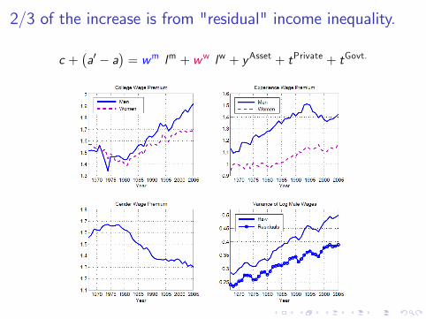
2/3 of the increase is from "residual" income inequality.
c +(a′ − a
)= wm lm + ww lw + yAsset + tPrivate + tGovt.

Inequality in labor earnings is increasing for men.
c +(a′ − a
)= wm lm + ww lw + yAsset + tPrivate + tGovt.

Inequality in household labor earnings is increasing.
c +(a′ − a
)= wm lm+ww lw + yAsset + tPrivate + tGovt.

Inequality in household labor earnings is increasing.
c +(a′ − a
)= wm lm+ww lw + yAsset + tPrivate + tGovt.
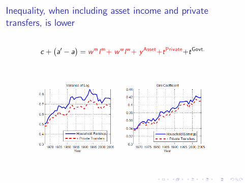
Inequality, when including asset income and privatetransfers, is lower
c +(a′ − a
)= wm lm+ ww lw+ yAsset+tPrivate+tGovt.

Inequality, when including taxes and government transfers,is even lower
c +(a′ − a
)= wm lm+ww lw+yAsset+tPrivate+tGovt.

Inequality in wealth is increasing
c +(a′ − a
)= wm lm + wm lw + yAsset + tPrivate + tGovt.

CEX: Inequality in expenditures is relatively flat.
c +(a′ − a
)= wm lm+ww lw+yAsset+tPrivate+tGovt.

CEX: Between/within group changes in inequality
c +(a′ − a
)= wm lm+ww lw+yAsset+tPrivate+tGovt.
Residual Variance Between-Group Variance
.05
0.0
5.1
.15
Cha
nge
in v
aria
nce
of lo
g co
nsum
ptio
n (o
r inc
ome)
1980 1985 1990 1995 2000 2005Y ear
0.0
2.0
4.0
6.0
8C
hang
e in
var
ianc
e of
log
cons
umpt
ion
(or i
ncom
e)
1980 1985 1990 1995 2000 2005Y ear
I Income inequality growth is largely within group.I Consumption inequality growth is largely between group.I Krueger and Perri (2006): These patterns are indicative ofeffective within-group insurance.

SummaryI Inequality is increasing
I First half of the sample: both 50-10 inequality and 90-50inequality
I Second half of the sample: 90-50 inequality only
I According to the CEX, expenditure inequality increases only alittle.
I Trends in earnings inequality are similar in the four datasetswe looked at.
I Micro data aggregates (increasingly) miss some componentsof income and expenditures.
I Also part of the same issue of the Review of EconomicDynamics: Analysis of inequality in Canada, GB, Germany,Italy, Spain, Sweden, Russia, Mexico.
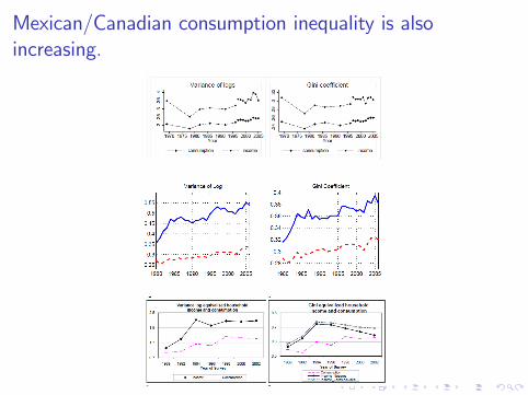
Mexican/Canadian consumption inequality is alsoincreasing.

Aguiar and BilsHas Consumption Inequality Mirrored Income Inequality?
.2.4
.6.8
1
Rat
io o
f Hou
seho
ld E
xpen
ditu
res,
CEX
vs. N
IPA
1980 1990 2000 2010Year

Aguiar and BilsHas Consumption Inequality Mirrored Income Inequality?
Health care
Serv ices
Goods.2
.4.6
.81
Rat
io o
f Hou
seho
ld E
xpen
ditu
res,
CEX
vs. N
IPA
1980 1990 2000 2010Year
Aguiar and BilsHas Consumption Inequality Mirrored Income Inequality?
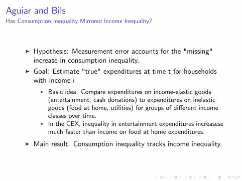
I Hypothesis: Measurement error accounts for the "missing"increase in consumption inequality.
I Goal: Estimate "true" expenditures at time t for householdswith income i
I Basic idea: Compare expenditures on income-elastic goods(entertainment, cash donations) to expenditures on inelasticgoods (food at home, utilities) for groups of different incomeclasses over time.
I In the CEX, inequality in entertainment expenditures increasesemuch faster than income on food at home expenditures.
I Main result: Consumption inequality tracks income inequality.

Income elasticities: β
Tobac
coFoo
d at h
ome
UtilitiesChil
dren's
cloth
ing
Applia
nces
All othe
r tran
sport
Health
care
Housin
g
Person
al ca
re
Vehicl
es
ShoesAlco
hol
Enterta
inmen
t equ
ipmen
t
Food o
ut
Adult c
lothin
g
Furnitu
reDom
estic
servi
ces
Educa
tion
Enterta
inmen
t fees
Cash c
ontrib
ution
s
.50
.51
1.5
22.
5β

Two main assumptions
1. Log-linear Engel curves:
log x∗hjt − log x̄∗jt = α∗jt + βj logX ∗ht + Γj Zh︸︷︷︸hh characteristics
+ ϕhjt︸︷︷︸taste shock
I Zh = number of earners (<2, 2+); household size; age (25-37,38-50, 51-64)
2. Household expenditures measurement error takes threecomponents:
xhjt = x∗hjteζhjt , where
ζhjt = ψjt + φit + υhjt
I ψjt : good-specific measurement errorI φit : income-group-specific measurement error.I Main assumption: υhjt , ϕhjt are orthogonal to householdcharacteristics or βj .

Growth of expenditures for high and low income groups
log xijt = αjt + φit + logX ∗itβj + εijt
clothes
alcbev
cashcont
chldrnclothes
educequpmt
foodawayfoodhome
ent
furniture
healthsvcs
trans
perscarehousing
shoes
tobacco
tvutilities auto
.25
0.2
5.5
.75
1Ex
pend
iture
Gro
wth
0 .5 1 1.5 2199496 E lasticities
clothes
alcbev
cashcont
chldrnclothes
educ
equpmtfoodawayfoodhome
ent
furniturehealth
svcs
trans
perscarehousing
shoes
tobacco
tvutilitiesauto
.5.2
50
.25
.5.7
51
Expe
nditu
re G
row
th
0 .5 1 1.5 2199496 E lasticities
I Left: log(xPoor,j ,2007xPoor,j ,1980
)= ∆αj ,2007−1980 + log
(X ∗Poor,2007X ∗Poor,1980
)βj
I Right: log(xRich,j ,2007xRich,j ,1980
)= ∆αj ,2007−1980 + log
(X ∗Rich,2007X ∗Rich,1980
)βj
I Slopes = −0.15, 0.28 ⇒ Expenditure inequality increases by43 log points.

Notes on Aguiar and Hurst (2007):"Measuring Trends in
Leisure: The Allocation ofTime over Five Decades"

The lecture so far
I Heathcote et al. (2010)I Household earnings inequality has been increasing since the1970s.
I Most of the increase is in residual ("within group") inequality.I Consumption inequality is basically flat. The small increase ismostly between-group inequality.
I Aguiar and Bils (2013)I Consumption inequality actually increases at a rate similar tothat of income inequality.

We care about utility from consumption expenditures......not consumption expenditures per se.
I We defined consumption ≡ f (x1, ..., xn) as a function ofexpenditures.
I Relevant budget constraint:∑i
pi · xi︸ ︷︷ ︸expenditures on good i
= W · tW︸ ︷︷ ︸labor income
+ V︸︷︷︸other income
I Becker (1965): Consumption consists of a bundle ofcommodities c1, ..., ci , ..., cn
I Commodities are a combination of market goods (xi ) and timeinputs (ti ): ci = φi (xi , ti )
I Extra budget constraint:∑i
ti︸︷︷︸time spent on commodity i
= T − tW

Research question and method
I Data on the evolution of tW have been readily available (inthe PSID, CPS, NLSY, etc...) for awhile. Not so for thecomponents of T − tW .
I How have the components of T − tW (time spent not workingin the market) changed over time
I ... on average?I ... for men vs. women?I ... for individuals in different income groups?
I Method: Combine time-use surveys from 1965 to 2003 (someresults extended to 2013).

Data Sources
I Use only retrospective diaries. Individuals badly estimate timeuse without time diaries.
I Robinson and Godbey (1997): Someone with a diary showing38 (55) hours/wk reports, in a retrospective interview, working40 (70+) hours/wk
I Americans Use of Time (1965-1966), Time Use in Economicand Social Accounts (1975-1976), Americans’Use of Time(1985), National Human Activity Pattern Survey (1992-1994).
I 2K-9K individuals per dataset.
I American Time Use SurveyI Annual, beginning in 2003.I 20K in 2003, somewhat fewer in other yearsI Can be linked to the CPS.

Main results and their implications
Two main findings:
1. Average time spent on leisure has gone up, by roughly 4 to 8hours
2. Dispersion in leisure time also increasing
2.1 90-10 difference in leisure time increases by 14 hours2.2 Less educated increase their leisure time more.
Implications:
I GDP growth may understate welfare growthI Looking at consumption expenditures may overstate thegrowth of inequality in the past few decades.

Demographic Change
>=College,6065
<HS,2129
0.0
1.0
2.0
3S
hare
in S
ampl
e
1970 1980 1990 2000 2010Year
I Most calculations "fix" demographic weights when computingaverages.
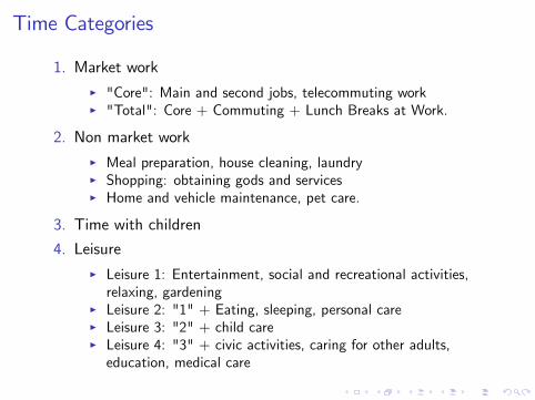
Time Categories
1. Market workI "Core": Main and second jobs, telecommuting workI "Total": Core + Commuting + Lunch Breaks at Work.
2. Non market workI Meal preparation, house cleaning, laundryI Shopping: obtaining gods and servicesI Home and vehicle maintenance, pet care.
3. Time with children
4. LeisureI Leisure 1: Entertainment, social and recreational activities,relaxing, gardening
I Leisure 2: "1" + Eating, sleeping, personal careI Leisure 3: "2" + child careI Leisure 4: "3" + civic activities, caring for other adults,education, medical care
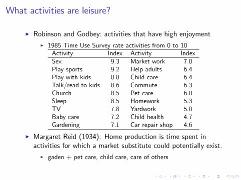
What activities are leisure?
I Robinson and Godbey: activities that have high enjoymentI 1985 Time Use Survey rate activities from 0 to 10
Activity Index Activity IndexSex 9.3 Market work 7.0Play sports 9.2 Help adults 6.4Play with kids 8.8 Child care 6.4Talk/read to kids 8.6 Commute 6.3Church 8.5 Pet care 6.0Sleep 8.5 Homework 5.3TV 7.8 Yardwork 5.0Baby care 7.2 Child health 4.7Gardening 7.1 Car repair shop 4.6
I Margaret Reid (1934): Home production is time spent inactivities for which a market substitute could potentially exist.
I gaden + pet care, child care, care of others

Time Spent in Market Work
2030
4050
Hou
rs
1970 1980 1990 2000 2010Year
I Core work declines 8 hours for men, up 3 hours for womenI "Non-core" market work declines 6 hours for men, 2 forwomen.

Time Spent in Home Production
1015
2025
3035
Hou
rs
1970 1980 1990 2000 2010Year
I Declines 11 hours for women, up 3 hours for men.

Time Spent with Children
02
46
8H
ours
1970 1980 1990 2000 2010Year
I Increases 2 hours for both men and women.

Leisure Time
3032
3436
38H
ours
1970 1980 1990 2000 2010Y ear
102
104
106
108
110
112
Hou
rs
1970 1980 1990 2000 2010Y ear
I "Leisure 2 measure" increases roughly by 6 hours for men, 5for women.

Leisure Time: Changing Demographic Weights
3032
3436
38H
ours
1970 1980 1990 2000 2010Y ear
102
104
106
108
110
112
Hou
rs
1970 1980 1990 2000 2010Y ear
I Slightly larger increase in leisure-2 time, with changingdemographic weights.
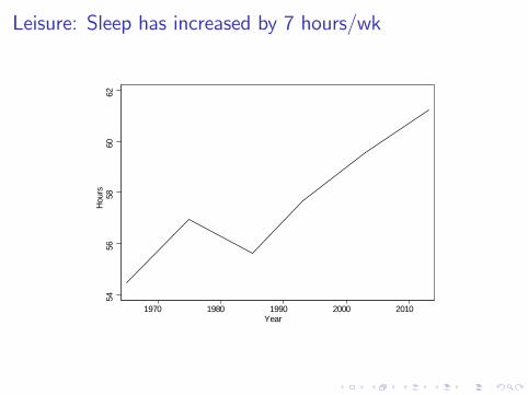
Leisure: Sleep has increased by 7 hours/wk
5456
5860
62H
ours
1970 1980 1990 2000 2010Year
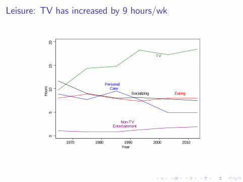
Leisure: TV has increased by 9 hours/wk
TV
PersonalCare
Socializing
NonTVEntertainment
Eating
05
1015
20H
ours
1970 1980 1990 2000 2010Year

Leisure: Reading has decreased by 4 hours/wk
Hobbies
Reading
Exercise
Gardenand Pet
All Other0
12
34
5H
ours
1970 1980 1990 2000 2010Year

Distribution of leisure time
Percentile 1965 1975 1985 1993 2003 201310 74.7 77.4 77.0 75.5 72.9 74.125 85.2 88.1 88.4 87.5 85.8 86.350 98.1 102.1 102.7 103.3 102.1 101.575 117.3 126 127.2 130.4 127.2 125.490 136.5 146.1 147.5 154.0 149.3 148.8Mean 102.0 107.0 107.5 110.8 110.2 109.2
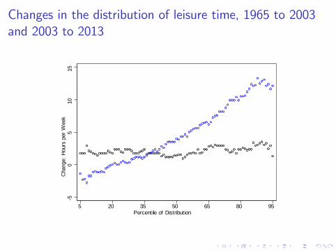
Changes in the distribution of leisure time, 1965 to 2003and 2003 to 2013
50
510
15C
hang
e: H
ours
per
Wee
k
5 20 35 50 65 80 95Percentile of Distribution

Changes in market time by education category
1525
3545
55H
ours
1970 1980 1990 2000 2010Y ear
1525
3545
55H
ours
1970 1980 1990 2000 2010Y ear
I Market time decreases most for less educated men.

Changes in leisure time by education category
100
105
110
115
120
Hou
rs
1970 1980 1990 2000 2010Y ear
100
105
110
115
120
Hou
rs
1970 1980 1990 2000 2010Y ear
I Leisure time increases most for less educated men.

Changes in leisure time by education category
Change:’65-’13
WholeSample
< HighSchool
HighSchool
SomeCollege
> College
Eating −0.64 −1.43 −0.62 −0.85 0.18Sleeping 6.78 8.17 7.98 6.84 3.57Pers. Care −4.10 −4.42 −4.40 3.52 −3.82TV 8.70 9.66 9.74 8.35 6.46Non-TV Ent. 0.84 0.98 0.95 0.82 0.57Socializing −4.96 −3.89 −4.95 −4.77 −6.06Hobbies −0.91 −0.89 −1.05 −0.77 −0.79Reading −3.75 −3.38 −3.75 −3.55 −4.23Exercise 0.77 0.47 0.48 0.58 1.66Garden 1.19 1.17 1.34 1.12 1.04All Other 1.33 3.05 1.35 0.92 0.18

Conclusion
I Average leisure increases by approx. 5 hours.
I 90th percentile in leisure distribution increases from 137 to149 hours per week; 10th percentile is flat at 74-75 hours.
I Leisure increases are concentrated in high school graduates,dropouts.
I Is it possible to estimate the functions, φi , f from thebeginning of the presentation (where, again,
c = f(φ1 (x1, t1) , ..., φi (xi , ti ) , ..., φn (xn, tn)
))
How does inequality in∑xi compare to inequality in c?

Notes on Aguiar et al. (2013):"Time Use During theGreat Recession"

Introduction
I Main Question: How does leisure and home production timevary over the business cycle?
I Because of data limitations, this question has been (up tonow) diffi cult to answer.
I ATUS begins in 2003. Now have dataset spanning only onerecession.
I Challenge to separate trend from cycle, draw inference from 1recession.
I Strategy: Use geographic (cross-state) variation on changes inmarket hours. Many more observations.

Outline
I Data.I Aggregate results.I Cross-state results.I Implications for Benhabib et al (1991).

Data
I American Time Use Survey: 2003 to 2013 (2010 in the paper).I Similar categorization to Aguiar and Hurst (2007), with a fewextra categories
I Market work. Approx 32 hoursI Other income generating activities. 10 minutesI Job search. 15 minutes;I Nonmarket work. 18 hoursI Leisure: TV, Socializing, Sleeping, Eating & Personal Care.108 hours.
I Child care. 4.5 hours.I Other: Education, Religion activities, Own medical care. 5hours.

Leisure has increased by roughly 3 hours
2003 2004 2005 2006 2007 2008 2009 2010 2011 2012 2013106
107
108
109
110
111
112
AllMenWomen
I About half of the increase from sleeping, the other half fromTV watching.

Leisure roughly 25 minutes above trend in the GR
2003 2004 2005 2006 2007 2008 2009 2010 2011 2012 2013106.5
107
107.5
108
108.5
109
109.5
110
110.5
111

Homework 15 minutes above trend in the GR
2003 2004 2005 2006 2007 2008 2009 2010 2011 2012 201316.5
17
17.5
18
18.5
19
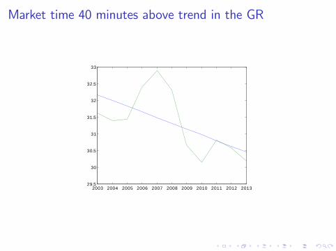
Market time 40 minutes above trend in the GR
2003 2004 2005 2006 2007 2008 2009 2010 2011 2012 201329.5
30
30.5
31
31.5
32
32.5
33

The method of de-trending matters
2003 2004 2005 2006 2007 2008 2009 2010 2011 2012 201329.5
30
30.5
31
31.5
32
32.5
33

The method of de-trending matters
Homework-Dev. from trend Leisure-Dev. from trend
2003 2004 2005 2006 2007 2008 2009 2010 2011 2012 20130.8
0.6
0.4
0.2
0
0.2
0.4
0.6
2003 2004 2005 2006 2007 2008 2009 2010 2011 2012 20131.2
1
0.8
0.6
0.4
0.2
0
0.2
0.4
0.6
I Deviation roughly 3× as large for homework, 40% higher forleisure, when using a quadratic trend.
I Not enough info from aggregate data ⇒ Use cross-statevariation.

Compare states with different market hours
∆τ jst = αj − βj∆τmarketst + εjst
s = state, t = period, j = activity
ALAL
AL
AL
AK
AKAK
AK
AZ
AZ
AZ
AZ
AR
ARAR
ARCACA CA
CA
COCO
CO COCTCT
CT
CT
DE
DE
DE
DEDC
DC
DC
DC
FL
FLFLFL
GA
GA
GA
GA HIHI
HI
HI
ID
ID
ID
ID
ILILIL
IL
IN
IN
IN
IN
IA
IA IA
IAKS
KSKS
KS
KY
KY
KY
KYLA
LALA
LAME
ME
ME
ME
MDMDMD
MD
MA
MA MA
MA
MI
MI
MI
MI
MNMN
MN
MN
MS
MSMS
MS
MO
MOMO
MO
MT
MTMT
MT
NE
NE
NENE
NVNV NV
NVNH
NHNH
NH
NJNJ
NJ NJ
NM
NM NM
NMNY
NY
NY
NY
NC
NC
NCNC
NDND
ND
ND
OH
OH OH
OH
OKOK OK
OK
OROR
ORORPA
PAPAPA
RI
RI
RI
RI
SCSCSC
SCSD
SDSD
SD
TNTN
TN
TNTX
TX
TX
TX
UT
UT
UT
UT
VT
VTVT
VT
VA
VA
VA
VAWA
WAWA
WA
WV
WV
WV
WV
WI WIWI
WIWY WY
WY
WY
AL
AK
AZ
ARCA CO
CT
DE
DC
FL GA
HI
ID
IL
IN
IA
KS
KYLAME MD
MA MIMNMS
MOMT
NE
NV
NHNJNM NYNC
ND
OH
OK
OR
PA
RI
SC
SD
TN
TX
UT
VT
VA
WAWV WI WY
20
10
010
20C
hang
e in
Lei
sure
Hou
rs
20 10 0 10 20 30Change in work hours
ALAL
AL
AL
AZ
AZAZ
AZ
AR
ARAR
CACA CACA
COCO
CO CO CTCTCT
FL
FLFLFLGA
GA
GA
GA
ID
ID
ILILIL
IL
IN
IN
IN
IN
IA
IA IA
KSKSKS
KY
KY
KY
KYLA
LALA
LAMD
MDMDMD
MA
MA MA
MA
MI
MI
MI
MI
MNMN
MN
MNMS
MSMS
MO
MOMO
MO
NE
NE
NE
NVNV NVNJ NJNJ NJ
NM
NM NM
NY
NY
NY
NY
NC
NC
NCNCOH
OH OH
OH
OKOK OKOROR
ORORPA
PAPAPASC
SCSCSC
TNTN
TN
TNTX
TX
TX
TX
UT
UT
UTVA
VA
VA
VAWA
WAWA
WA
WV
WV
WV
WI WIWI
WI
AL
AZ
ARCA CO
CT
FL GAIL
IN
IA
KSKY
LAMDMA MIMNMS
MO
NENV
NJNM NYNC
OH
OK
ORPASCTN
TX
UT
VAWAWI
20
10
010
2030
Cha
nge
in L
eisu
re H
ours
20 10 0 10 20 30Change in work hours
β leisure ≈ 0.55

Compare states with different market hours
∆τ jst = αj − βj∆τmarketst + εjst
s = state, t = period, j = activity
AL
AL
ALAL
AK
AK AK
AK
AZ
AZAZ
AZAR
AR AR
ARCACA
CA
CACO
COCO
CO
CTCTCT
CTDE
DE
DEDE
DC
DC
DC
DCFLFL
FLFL
GA
GAGA
GA
HI
HI
HI
HI
ID
ID
ID
ID
ILIL
ILILIN
ININ
IN
IA
IAIA
IA
KS KSKS
KS
KY
KY
KYKYLA
LA
LA
LA
ME
ME
ME
ME MDMDMDMDMA
MA
MA
MAMI MI
MI
MI
MNMN
MNMN
MS
MSMSMSMO
MOMOMO
MT
MTMT
MT
NE
NE
NE
NE
NV
NV
NV
NV
NH
NHNH
NH
NJ
NJNJ
NJ
NM
NMNM
NM
NYNY NY
NY
NC
NCNC
NC
ND
ND
ND
ND
OHOH OHOH
OK
OK
OK
OKOR
OR
OR
OR
PA
PA PAPA
RI
RIRI
RI
SC
SCSC SC
SD
SD
SDSD
TN
TN TNTNTX
TX
TXTX
UT
UTUT
UT
VT
VT
VT
VT
VA
VAVA
VA
WA
WAWA
WAWV WVWV
WV
WI
WI
WI
WI
WY
WY
WY
WY
AL
AK
AZ
ARCA
CO
CT
DE
DCFLGA
HIID IL
IN
IA
KS
KY
LA
MEMD
MA
MI
MNMS
MO
MT
NE NV
NHNJ
NMNY
NC
ND
OHOKOR
PA
RI
SC
SD
TNTX
UT
VT
VAWA
WV
WI
WY
10
010
20C
hang
e in
Hom
e W
ork
Hou
rs
20 10 0 10 20 30Change in work hours
AL
AL
ALAL
AZ
AZAZ
AZAR
AR AR
CACA
CA
CACO
COCO
CO
CTCTCT FL
FLFL
FL
GA
GAGA
GA
ID
IDILIL
ILILIN
ININ
IN
IA
IAIA
KS KSKS
KY
KY
KYKYLA
LA
LA
LA
MDMDMDMD
MAMA
MA
MAMI MI
MI
MI
MNMN
MN
MN
MS
MSMS
MO
MOMOMO
NE
NE
NE NV
NV
NV
NJ
NJNJ
NJ
NM
NMNM
NYNY NY
NY
NC
NCNC
NC
OHOH OHOH
OK
OK
OK
OR
OR
OR
OR
PA
PAPA
PA
SC
SCSC SC
TN
TNTN
TNTX
TX
TXTX
UT
UTUT
VA
VAVA
VA
WA
WAWA
WAWV WV
WV
WI
WI
WI
WI
AL
AZ
ARCA
CO
CTFL
GAIL
IN
IA
KS
KY
LA
MD
MA
MI
MNMS
MO
NE NV
NJ
NMNY
NC
OHOKOR
PASC
TNTX
UT
VAWA
WI
10
010
20C
hang
e in
Hom
e W
ork
Hou
rs20 10 0 10 20 30
Change in work hours
βhome work ≈ 0.30

More Comparisons
SampleMean
β̂unweighted
β̂weighted
Other income-generating activities
0.14 7.9 0.9
Job search 0.23 2.8 1.5Child care 3.36 1.6 4.2Nonmarket work 13.03 29.1 31.8Core home production 6.91 13.2 13.3Home ownership activities 1.57 4.4 5.8
Leisure 79.52 55.6 52.7TV watching 13.07 12.4 13.2Socializing 5.61 8.5 7.2Sleeping 43.85 14.8 17.9Eating and personal care 9.75 0.5 -0.1Other leisure 7.23 19.5 14.4
Other 3.72 10.1 8.9

How to identify e from cross-state data?
I Simulate Benhabib, Rogerson, Wright model; 51 "states" and58 years of data (discard first 50 years).
I From the simulated data, regress
∆τhomest = αj − βj∆τmarketst + εjst
I Version 1 (2): Leisure includes (excludes) sleep.I Now try different values of e
VersionModele = 0.8
Modele = 0.5
DataFull Sample
DataRecession
1 0.74 0.46 0.50 0.572 0.48 0.20 0.39 0.47

How to identify "e" from cross-state data?
∆τhomest = αj − βj∆τmarketst + εjst
I σ ∈ [2.5, 4] ⇐⇒ e ∈ [0.6, 0.75]

Connections to structural transformation?
I Different groups of individuals (women, college+ educated)had faster labor income growth. Is this related to
I Increase in the prominence of services? (Problem Set 3)I Decline in the price of capital (particularly computer-relatedinvestment goods)?
I Time spent in home production declines (and women’s laborforce participation increases)
I ⇐declines in relative price of durable consumption goods?
I Capital share of income is increasing... Implications forinequality? (Problem Set 1)

Connections to other macro issues
I This paper: One example application of time use surveys:Reexamining changes in inequality
I One other example: Babcock and Marks (2010) examine timediaries of college students. Hours spent studying declines bya third between 1961 and 2003 ⇒ Declining production ofhuman capital.
I Data from other countries are also readily available:Multinational Time Use Survey (MTUS) is a harmonizeddataset of ˜ 20 (mainly developed) countries.
I Survey of Unemployed Workers in New Jersey: Individual-levelpanel of time use.