COST-CAUSALITY BASED TARIFFS FOR

DISTRIBUTION NETWORKS WITH DISTRIBUTED

GENERATION

author

Jesus Mario Vignolo

SUBMITTED IN PARTIAL FULFILLMENT OF THE

REQUIREMENTS FOR THE DEGREE OF

DOCTOR OF ELECTRICAL ENGINEERING

AT

UNIVERSIDAD DE LA REPUBLICA ORIENTAL DEL URUGUAY

JULIO HERRERA Y REISSIG 565, MONTEVIDEO, URUGUAY

c© Copyright by Jesus Mario Vignolo, 2007

Email: jesus@fing.edu.uy

.

ii

UNIVERSIDAD DE LA REPUBLICA ORIENTAL DEL URUGUAY

INSTITUTO DE INGENIERıA ELECTRICA

The undersigned hereby certify that they have read and recommend

to Facultad de Ingenierıa for acceptance a thesis entitled “Cost-causality

Based Tariffs for Distribution Networks with Distributed

Generation” by Jesus Mario Vignolo in partial fulfillment of the

requirements for the degree of Doctor of Electrical Engineering.

Date: October 2007

Thesis Director:Paul M. Sotkiewicz

Academic Director:Gonzalo Casaravilla

External Examiner:Hugh Rudnick

Mario Bergara

Jorge Vidart

Pablo Monzon

Jose Cataldo

iii

ISSN: 1510 7264 Reporte Tecnico N o....

Universidad de la Republica

Facultad de Ingenierıa

Julio Herrera y Reissig 565

Montevideo, CP 11300

Uruguay

iv

UNIVERSIDAD DE LA REPUBLICA ORIENTAL DEL

URUGUAY

Date: October 2007

Author: Jesus Mario Vignolo

Title: Cost-causality Based Tariffs for Distribution

Networks with Distributed Generation

Institute: Ingenierıa Electrica

Degree: Doctor of Electrical Engineering (PhD.)

Permission is herewith granted to Universidad de la Republica Orientaldel Uruguay to circulate and to have copied for non-commercial purposes, atits discretion, the above title upon the request of individuals or institutions.

Signature

The author reserves other publication rights, and neither the thesis norextensive extracts from it may be printed or otherwise reproduced without the author’swritten permission.

The author attests that permission has been obtained for the use of anycopyrighted material appearing in this thesis (other than brief excerpts requiringonly proper acknowledgement in scholarly writing) and that all such use is clearlyacknowledged.

v

.

vi

Index

Index ix

Abstract xi

Acknowledgements xiii

1 Distribution Networks with Distributed Generation: Technical and

Commercial Issues 1

1.1 Introduction: Some History and Evolution Towards Distributed Gen-

eration . . . . . . . . . . . . . . . . . . . . . . . . . . . . . . . . . . . 1

1.2 What is Distributed Generation? . . . . . . . . . . . . . . . . . . . . 7

1.3 DG Technologies . . . . . . . . . . . . . . . . . . . . . . . . . . . . . 9

1.3.1 Reciprocating engines . . . . . . . . . . . . . . . . . . . . . . . 9

1.3.2 Simple cycle gas turbines . . . . . . . . . . . . . . . . . . . . . 9

1.3.3 Microturbines . . . . . . . . . . . . . . . . . . . . . . . . . . . 11

1.3.4 Fuel cells . . . . . . . . . . . . . . . . . . . . . . . . . . . . . . 11

1.3.5 Renewable technologies . . . . . . . . . . . . . . . . . . . . . . 11

1.3.6 The role of natural gas and petroleum prices in cost estimates 11

1.4 Potential Benefits of Distributed Generation . . . . . . . . . . . . . . 12

1.4.1 Combined heat and power applications . . . . . . . . . . . . . 12

1.4.2 Impact of DG on reliability (security of supply) . . . . . . . . 14

1.4.3 Impact of DG on network losses and usage . . . . . . . . . . . 14

1.4.4 Impact of DG on voltage regulation . . . . . . . . . . . . . . . 17

1.4.5 Potential to postpone generation investment . . . . . . . . . . 20

1.4.6 Potential electricity market benefits . . . . . . . . . . . . . . . 21

1.4.7 Potential environmental benefits . . . . . . . . . . . . . . . . . 22

1.5 Policies and Chapter Concluding Remarks . . . . . . . . . . . . . . . 22

2 Current Schemes for Distribution Pricing 23

2.1 Costs in the Distribution Business . . . . . . . . . . . . . . . . . . . . 23

2.1.1 Capital costs . . . . . . . . . . . . . . . . . . . . . . . . . . . 23

2.1.2 Operational costs . . . . . . . . . . . . . . . . . . . . . . . . . 25

2.1.3 Fixed and variable costs . . . . . . . . . . . . . . . . . . . . . 25

vii

2.2 Traditional Cost Allocation Methodologies . . . . . . . . . . . . . . . 25

2.2.1 Average losses . . . . . . . . . . . . . . . . . . . . . . . . . . . 26

2.2.2 Allocation of fixed costs . . . . . . . . . . . . . . . . . . . . . 27

2.2.3 Full charges . . . . . . . . . . . . . . . . . . . . . . . . . . . . 28

2.2.4 The effect of traditional cost allocation methodologies on the

development of DG . . . . . . . . . . . . . . . . . . . . . . . . 28

2.3 Present Pricing and Policy Approaches with respect to DG . . . . . . 29

2.4 Chapter Concluding Remarks . . . . . . . . . . . . . . . . . . . . . . 30

3 A New Distribution Tariff Framework for Efficient Enhancing DG 31

3.1 Nodal Pricing for Distribution Networks . . . . . . . . . . . . . . . . 31

3.1.1 Full marginal losses from nodal prices . . . . . . . . . . . . . . 33

3.1.2 Reconciliated marginal losses . . . . . . . . . . . . . . . . . . 34

3.2 Allocation of Fixed Costs: The Amp-mile Methodology . . . . . . . . 35

3.2.1 Extent-of-use methods for distribution networks . . . . . . . . 35

3.2.2 The Amp-mile methodology: Allocation strategy and descrip-

tion of charges . . . . . . . . . . . . . . . . . . . . . . . . . . . 37

3.2.3 Extent-of-use measurement defined for Amp-mile . . . . . . . 40

3.2.4 Defining costs for Amp-mile . . . . . . . . . . . . . . . . . . . 42

3.2.5 Defining time differentiated charges per MWh for Amp-mile . 43

3.2.6 Fixed charges based on extent-of-use at system peak . . . . . 44

3.2.7 Nonlocational charges under Amp-mile . . . . . . . . . . . . . 46

3.3 Combining Nodal Pricing with Amp-mile Charges . . . . . . . . . . . 48

3.4 Chapter Concluding Remarks . . . . . . . . . . . . . . . . . . . . . . 49

4 Application of Combined Nodal Pricing and Amp-mile to Distribu-

tion Networks 51

4.1 General Considerations . . . . . . . . . . . . . . . . . . . . . . . . . . 51

4.2 Application: System Characteristics . . . . . . . . . . . . . . . . . . . 51

4.3 Simulations and Results for Controllable and Intermittent DG . . . . 52

4.4 Amp-mile: Time Differentiated Charges vs. Fixed Yearly Charges at

Coincident Peak . . . . . . . . . . . . . . . . . . . . . . . . . . . . . . 59

4.4.1 Time differentiated per unit locational charges . . . . . . . . . 61

4.4.2 Fixed, coincident peak locational charges . . . . . . . . . . . . 64

4.5 Chapter Concluding Remarks . . . . . . . . . . . . . . . . . . . . . . 66

5 Towards a New Tariff Framework for Distribution Networks 81

5.1 General Considerations . . . . . . . . . . . . . . . . . . . . . . . . . . 81

5.2 Tariff Decomposition Results . . . . . . . . . . . . . . . . . . . . . . . 81

5.2.1 Averaging losses and network costs . . . . . . . . . . . . . . . 82

5.2.2 Averaging losses and coincident peak network costs . . . . . . 82

5.2.3 Averaging losses and Amp-mile network charges . . . . . . . . 84

5.2.4 Reconciliated marginal losses and Amp-mile network charges . 86

viii

5.2.5 Full marginal losses and Amp-mile network charges . . . . . . 88

5.2.6 Benchmark average cost tariff vs. proposed cost causation based

tariff . . . . . . . . . . . . . . . . . . . . . . . . . . . . . . . . 90

5.3 Chapter Concluding Remarks . . . . . . . . . . . . . . . . . . . . . . 92

6 General Conclusions and Results 95

Bibliography 100

A Power Flow and Analytical Derivatives Calculation 107

A.0.1 The iterative algorithm . . . . . . . . . . . . . . . . . . . . . . 110

A.0.2 Derivatives calculation . . . . . . . . . . . . . . . . . . . . . . 110

B Published papers at IEEE 115

ix

x

Abstract

Doctor of Electrical Engineering Thesis“Cost-causality Based Tariffs for Distribution Networkswith Distributed Generation”Author: Jesus Mario Vignolo.Thesis Director: Paul M. Sotkiewicz.Academic Director: Gonzalo Casaravilla.Universidad de la Republica - Uruguay - October de 2007

Around the world, the amount of distributed generation (DG) deployed in dis-

tribution networks is increasing. It is well understood that DG has the potential to

reduce network losses, decrease network utilization, postpone new investment in cen-

tral generation, increase security of supply, and contribute to service quality through

voltage regulation. In addition, DG can increase competition in electricity markets,

and for the case of renewable DG provide environmental benefits.

The increasing penetration of DG in the power systems worldwide has changed

the concept of the distribution networks. Traditionally the costs of these networks

were allocated only to demand customers, not generation because these networks were

viewed as serving demand only. In this sense, traditional distribution networks were

considered passive networks unlike transmission networks which serve both generation

and demand and have always been considered active networks. The introduction of

DG transforms a distribution network from a passive network into an active network.

Present tariffs schemes at distribution level have been conceived using the tradi-

tional concept of distribution and do not recognize the new situation. Tariffs have

been, and actually are, designed for networks which only have loads connected. These

tariffs that normally average costs among network users are not able to capture the

real costs and benefits of some customers like DG. Consequently, traditional tariffs

schemes at the distribution level can affect the competitiveness of DG and can actually

hinder or stop its development.

In this work a cost-causality based tariff is proposed for distribution taking into

account new distribution networks tend to be active networks, much like transmis-

sion. Two concepts based on the same philosophy used for transmission pricing are

proposed. The first is nodal pricing for distribution networks, which is an economi-

cally efficient pricing mechanism for short term operation with which there is a great

deal of experience and confidence from its use at transmission level. The second is

xi

xii

an extent-of-use method for the allocation of fixed costs that uses marginal changes

in a circuit’s current flow with respect to active and reactive power changes in nodes,

and thus was called Amp-mile method. The proposed scheme for distribution pricing

results to give adequate price signals for location and operation for both generation

and loads. An example application based on a typical 30 kV rural radial network in

Uruguay is used to show the properties of the proposed methodology.

Acknowledgements

This work could not have been possible without the continuous support of my family

and friends.

I would like to specially thank Dr. Gonzalo Casaravilla and Dr. Paul Sotkiewicz,

who believed in this project from the very beginning and gave their unconditional

support to me over the past four years.

xiii

Chapter 1

Distribution Networks withDistributed Generation: Technicaland Commercial Issues1

1.1 Introduction: Some History and Evolution To-

wards Distributed Generation

When the electricity supply industry (ESI) was first developed, municipally owned

companies supplied electric energy in a community and installed generators located

according to the distribution needs. The ESI began its history using distributed

generation (DG), or generation directly installed in the distribution network, very

near to consumers (CIGRE WG 37.23, 1999). Plans for new generation capacity

were developed to satisfy demand, with a certain reserve margin for security reasons.

Over time, increasing electricity demand was satisfied by installing large genera-

tion plants, generally near the primary energy sources (e.g., coal mines, rivers, etc.).

The rationale behind this was the great efficiency difference due to economies of scale

between one big generation plant and several small ones. In addition, the resulting

system reserve margins were smaller with large central stations than with distributed

resources. The result was the traditional concept of the electric power system (EPS),

as shown in Figure1.1. In an EPS with big generators, energy must necessarily be

transported to the demand using very high voltage networks. This development ra-

tionale has been systematically promoted by the fact that the transmission system

costs have been smaller than the cost savings produced by the economies of scale

1This chapter draws heavily in both text and concept from the published version of(Sotkiewicz, P.M. and Vignolo, J.M. 2/07, 2007).

1

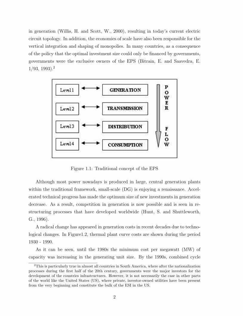
in generation (Willis, H. and Scott, W., 2000), resulting in today’s current electric

circuit topology. In addition, the economies of scale have also been responsible for the

vertical integration and shaping of monopolies. In many countries, as a consequence

of the policy that the optimal investment size could only be financed by governments,

governments were the exclusive owners of the EPS (Bitrain, E. and Saavedra, E.

1/93, 1993).2

Figure 1.1: Traditional concept of the EPS

Although most power nowadays is produced in large, central generation plants

within the traditional framework, small-scale (DG) is enjoying a renaissance. Accel-

erated technical progress has made the optimum size of new investments in generation

decrease. As a result, competition in generation is now possible and is seen in re-

structuring processes that have developed worldwide (Hunt, S. and Shuttleworth,

G., 1996).

A radical change has appeared in generation costs in recent decades due to techno-

logical changes. In Figure1.2, thermal plant curve costs are shown during the period

1930 - 1990.

As it can be seen, until the 1980s the minimum cost per megawatt (MW) of

capacity was increasing in the generating unit size. By the 1990s, combined cycle

2This is particularly true in almost all countries in South America, where after the nationalizationprocesses during the first half of the 20th century, governments were the major investors for thedevelopment of the countries infrastructures. However, it is not necessarily the case in other partsof the world like the United States (US), where private, investor-owned utilities have been presentfrom the very beginning and constitute the bulk of the ESI in the US.

2

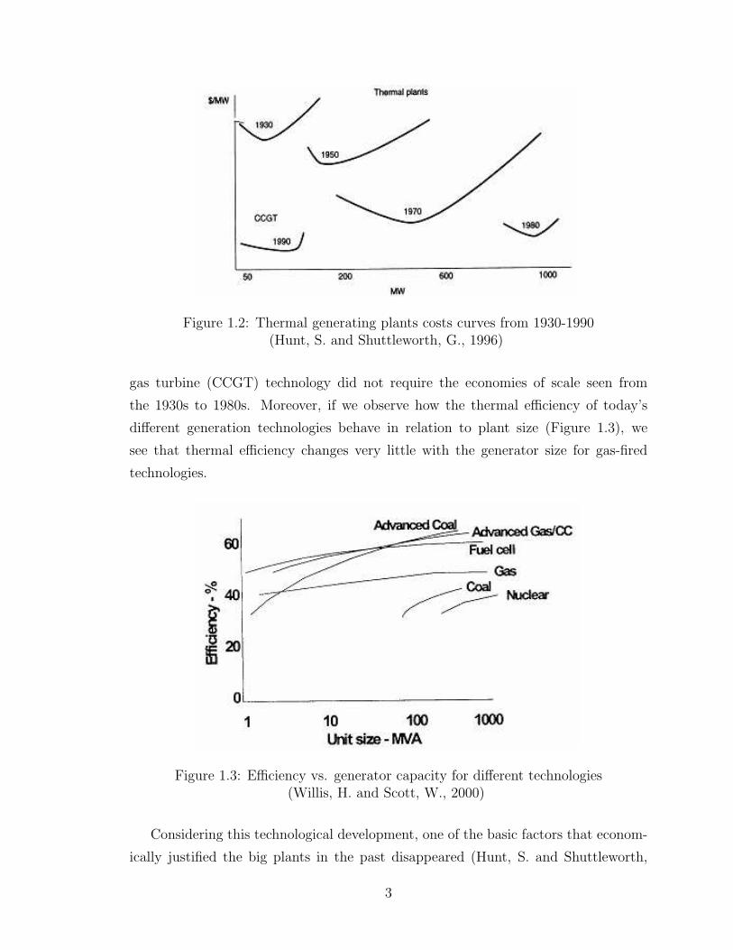
Figure 1.2: Thermal generating plants costs curves from 1930-1990(Hunt, S. and Shuttleworth, G., 1996)

gas turbine (CCGT) technology did not require the economies of scale seen from

the 1930s to 1980s. Moreover, if we observe how the thermal efficiency of today’s

different generation technologies behave in relation to plant size (Figure 1.3), we

see that thermal efficiency changes very little with the generator size for gas-fired

technologies.

Figure 1.3: Efficiency vs. generator capacity for different technologies(Willis, H. and Scott, W., 2000)

Considering this technological development, one of the basic factors that econom-

ically justified the big plants in the past disappeared (Hunt, S. and Shuttleworth,

3

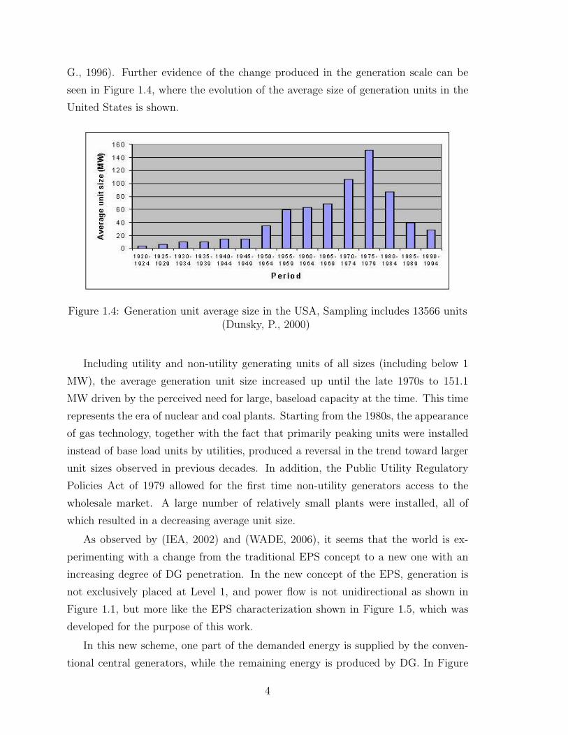
G., 1996). Further evidence of the change produced in the generation scale can be

seen in Figure 1.4, where the evolution of the average size of generation units in the

United States is shown.

Figure 1.4: Generation unit average size in the USA, Sampling includes 13566 units(Dunsky, P., 2000)

Including utility and non-utility generating units of all sizes (including below 1

MW), the average generation unit size increased up until the late 1970s to 151.1

MW driven by the perceived need for large, baseload capacity at the time. This time

represents the era of nuclear and coal plants. Starting from the 1980s, the appearance

of gas technology, together with the fact that primarily peaking units were installed

instead of base load units by utilities, produced a reversal in the trend toward larger

unit sizes observed in previous decades. In addition, the Public Utility Regulatory

Policies Act of 1979 allowed for the first time non-utility generators access to the

wholesale market. A large number of relatively small plants were installed, all of

which resulted in a decreasing average unit size.

As observed by (IEA, 2002) and (WADE, 2006), it seems that the world is ex-

perimenting with a change from the traditional EPS concept to a new one with an

increasing degree of DG penetration. In the new concept of the EPS, generation is

not exclusively placed at Level 1, and power flow is not unidirectional as shown in

Figure 1.1, but more like the EPS characterization shown in Figure 1.5, which was

developed for the purpose of this work.

In this new scheme, one part of the demanded energy is supplied by the conven-

tional central generators, while the remaining energy is produced by DG. In Figure

4

Figure 1.5: The new EPS concept

1.5, a distinction is made between DG and DG - self-generation. The latter cor-

responds to those cases in which consumers produce electric energy for themselves,

rather than for distribution. However, it may be observed that this type of generation

is also considered DG.

Currently, most of the electricity produced in the world is generated in large

generating stations, but some electricity is produced by DG resources. In contrast

to large generating stations, DG can be used by a local distribution utility or by

an independent producer to supply power directly to the local distribution network

close to demand, or DG produces power on site for direct use by an individual cus-

tomer. DG technologies include engines, small turbines, fuel cells, and photovoltaic

systems. Although they represent a small share of the electricity market, DG tech-

nologies already play a key role: for applications in which reliability is crucial, as a

source of emergency capacity and as an alternative to expansion of a local network.

In some markets, DG technologies are actually displacing more costly grid-supplied

electricity.3 Government policies favoring combined heat and power (CHP) genera-

tion, renewable energy, and technological development will likely assure the continued

growth of DG.

3In many of these cases, grid-supplied power is not provided at the correct price, leading to this“bypass ”of the grid.

5

The Working Group 37.23 of the CIGRE (Conseil International des Grands Reseaux

Electriques - International Council on Large Electric Systems) (CIGRE WG 37.23,

1999) has summarized the reasons for an increasing share of DG in different countries.

The aspects included in the report are the following:

• DG technologies are mature, readily available, and modular in a capacity range

from 100 kW to 150 MW.

• The generation can be sited close to customer load, which may decrease trans-

mission costs.

• Sites for smaller generators are easier to find.

• No large and expensive heat distribution systems are required for local systems

fed by small CHP-units.

• Natural gas, often used as fuel for DG, was expected to be readily available in

most customer load centers and was expected to have stable prices.

• Gas based units are expected to have short lead times and low capital costs

compared to large central generation facilities.

• Higher efficiency is achievable in cogeneration and combined cycle configurations

leading to low operational costs.

• Politically motivated regulations, e.g., subsidies and high reimbursement tariffs

for environmentally friendly technologies, or public service obligations, e.g., with

the aim to reduce CO2 - emissions, lead to economically favorable conditions.

• In some systems, DG competes with the energy price paid by the consumer

without contributing to or paying for system services which gives DG an ad-

vantage compared to large generation facilities.

• Financial institutions are often willing to finance DG-projects since economics

are often favorable.

• Unbundled systems with more competition on the generation market provide

additional chances for industry and others to start a generation business.

• Customers demand for “green power” is increasing.4

4This has it also been cited by (Hyde, D., 1998).

6

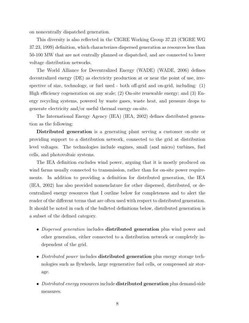
Information provided by the World Alliance for Decentralized Energy (WADE),

shows the share of decentralized energy in different countries for 2005 (Figure 1.6).

The share of decentralized power generation in the world market has increased to 10.4

percent in 2005, up from 7 percent in 2002.

Figure 1.6: Decentralized energy share in the world(WADE, 2006)

1.2 What is Distributed Generation?

Many terms have emerged to describe power that comes from sources other than

from large, centrally dispatched generating units connected to a high voltage trans-

mission system or network. In fact, there is no clear consensus as to what constitutes

distributed generation (IEA, 2002), (CIRED, 1999).

The CIRED (Congres International des Reseaux Electriques de Distribution - In-

ternational Conference on Electricity Distribution) Working Group 4 (CIRED, 1999)

created a survey of 22 questions which sought to identify the current state of dispersed

generation in various CIRED-member countries. Response showed no agreement on a

definition of dispersed generation with some countries using a voltage level definition,

while others considered direct connection to consumer loads. Other definitions relied

on the type of prime mover (e.g., renewable or cogeneration), while others were based

7

on noncentrally dispatched generation.

This diversity is also reflected in the CIGRE Working Group 37.23 (CIGRE WG

37.23, 1999) definition, which characterizes dispersed generation as resources less than

50-100 MW that are not centrally planned or dispatched, and are connected to lower

voltage distribution networks.

The World Alliance for Decentralized Energy (WADE) (WADE, 2006) defines

decentralized energy (DE) as electricity production at or near the point of use, irre-

spective of size, technology, or fuel used - both off-grid and on-grid, including: (1)

High efficiency cogeneration on any scale; (2) On-site renewable energy; and (3) En-

ergy recycling systems, powered by waste gases, waste heat, and pressure drops to

generate electricity and/or useful thermal energy on-site.

The International Energy Agency (IEA) (IEA, 2002) defines distributed genera-

tion as the following:

Distributed generation is a generating plant serving a customer on-site or

providing support to a distribution network, connected to the grid at distribution

level voltages. The technologies include engines, small (and micro) turbines, fuel

cells, and photovoltaic systems.

The IEA definition excludes wind power, arguing that it is mostly produced on

wind farms usually connected to transmission, rather than for on-site power require-

ments. In addition to providing a definition for distributed generation, the IEA

(IEA, 2002) has also provided nomenclature for other dispersed, distributed, or de-

centralized energy resources that I outline below for completeness and to alert the

reader of the different terms that are often used with respect to distributed generation.

It should be noted in each of the bulleted definitions below, distributed generation is

a subset of the defined category.

• Dispersed generation includes distributed generation plus wind power and

other generation, either connected to a distribution network or completely in-

dependent of the grid.

• Distributed power includes distributed generation plus energy storage tech-

nologies such as flywheels, large regenerative fuel cells, or compressed air stor-

age.

• Distributed energy resources include distributed generation plus demand-side

measures.

8

• Decentralized power refers to a system of distributed energy resources connected

to a distribution network.

For the purpose of this work, distributed generation will be defined as generation

used on-site and/or connected to the distribution network irrespective of size, tech-

nology, or fuel used. This nomenclature encompasses the definition in (IEA, 2002).

However, unlike the IEA criteria, wind power is included if it is connected to the

distribution network close to the demand.

1.3 DG Technologies

1.3.1 Reciprocating engines

Reciprocating engines, according to (IEA, 2002), are the most common form of dis-

tributed generation. This is a mature technology that can be fueled by either diesel

or natural gas, though the majority of applications are diesel fired. The technology

is capable of thermal efficiencies of just over 40 percent for electricity generation and

relatively low capital costs but relatively high running costs as shown in Table 1.1.

The technology is also suitable for back-up generation as it can be started up quickly

and without the need for grid-supplied power. When fueled by diesel, this technology

has the highest nitrogen oxide (NOx) and carbon dioxide (CO2) emissions of any of

the distributed generation technologies considered here as seen in Table 1.2.

1.3.2 Simple cycle gas turbines

This technology is also mature deriving from the development and use of turbines as

jet engines. The electric utility industry uses simple cycle gas turbines as units to

serve peak load, and these turbines generally tend to be larger in size. Simple cycle

gas turbines have the same operating characteristics as reciprocating engines in terms

of start-up and the ability to start independently of grid-supplied power making them

suitable as well for back-up power needs. This technology is also often run in CHP

applications which can increase overall thermal efficiency. Capital costs are on par

with natural gas engines as seen in Table 1.1 with a similar operating and levelized

cost profile. The technology tends to be cleaner as it is designed to run on natural

gas as seen in Table 1.2.

9

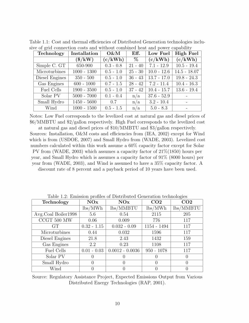
Table 1.1: Cost and thermal efficiencies of Distributed Generation technologies inclu-sive of grid connection costs and without combined heat and power capability

Technology Installation O&M Eff. Low Fuel High Fuel($/kW) (c/kWh) % (c/kWh) (c/kWh)

Simple C. GT 650-900 0.3 - 0.8 21 - 40 7.1 - 12.9 10.5 - 19.4Microturbines 1000 - 1300 0.5 - 1.0 25 - 30 10.0 - 12.6 14.5 - 18.07Diesel Engines 350 - 500 0.5 - 1.0 36 - 43 13.7 - 17.0 19.8 - 24.3Gas Engines 600 - 1000 0.7 - 1.5 28 - 42 7.2 - 11.4 10.4 - 16.3Fuel Cells 1900 - 3500 0.5 - 1.0 37 - 42 10.4 - 15.7 13.6 - 19.4Solar PV 5000 - 7000 0.1 - 0.4 n/a 37.6 - 52.9 -

Small Hydro 1450 - 5600 0.7 n/a 3.2 - 10.4 -Wind 1000 - 1500 0.5 - 1.5 n/a 5.0 - 8.3 -

Notes: Low Fuel corresponds to the levelized cost at natural gas and diesel prices of$6/MMBTU and $2/gallon respectively. High Fuel corresponds to the levelized cost

at natural gas and diesel prices of $10/MMBTU and $3/gallon respectively.Sources: Installation, O&M costs and efficiencies from (IEA, 2002) except for Windwhich is from (USDOE, 2007) and Small Hydro from (WADE, 2003). Levelized costnumbers calculated within this work assume a 60% capacity factor except for SolarPV from (WADE, 2003) which assumes a capacity factor of 21%(1850) hours peryear, and Small Hydro which is assumes a capacity factor of 91% (8000 hours) peryear from (WADE, 2003), and Wind is assumed to have a 35% capacity factor. A

discount rate of 8 percent and a payback period of 10 years have been used.

Table 1.2: Emission profiles of Distributed Generation technologiesTechnology NOx NOx CO2 CO2

lbs/MWh lbs/MMBTU lbs/MWh lbs/MMBTUAvg.Coal Boiler1998 5.6 0.54 2115 205

CCGT 500 MW 0.06 0.009 776 117GT 0.32 - 1.15 0.032 - 0.09 1154 - 1494 117

Microturbines 0.44 0.032 1596 117Diesel Engines 21.8 2.43 1432 159Gas Engines 2.2 0.23 1108 117Fuel Cells 0.01 - 0.03 0.0012 - 0.0036 950 - 1078 117Solar PV 0 0 0 0

Small Hydro 0 0 0 0Wind 0 0 0 0

Source: Regulatory Assistance Project, Expected Emissions Output from VariousDistributed Energy Technologies (RAP, 2001).

10

1.3.3 Microturbines

This technology takes simple cycle gas technology and scales it down to capacities of

50-100 kW. The installed costs per kW of capacity are greater than for gas turbines,

and the efficiencies are lower as well as seen in Table 1.1. However, it is much quieter

than a gas turbine and has a much lower emissions profile than gas turbines as seen in

Table 1.2. The possibility also exists for microturbines to be used in CHP applications

to improve overall thermal efficiencies.

1.3.4 Fuel cells

Fuel cells are a relatively new technology and can run at electrical efficiencies compa-

rable to other mature technologies. Fuels cells have the highest capital cost per kW of

capacity among fossil-fired technologies and consequently have the highest levelized

costs as seen in Table 1.1. Offsetting that, the emission footprint of fuel cells is much

lower than the other technologies as seen in Table 1.2.

1.3.5 Renewable technologies

There are three major types of renewable energy technologies we discuss here: solar

photovoltaic (PV), small hydro, and wind. These technologies are intermittent in

that each are dependent upon either the sun, river flows, or wind, but also have no

fuel costs and have a zero emissions profile as seen in Table 1.2. The intermittency

of each of these technologies make them unsuitable for back-up power. The capital

costs vary significantly among the technologies, and operating conditions over the

year affect their respective levelized costs. Solar PV is by far the most expensive in

both capital costs and levelized costs as seen in Table 1.1. Capital costs for wind

are much lower, but levelized costs are in the range of more traditional technologies

as seen in Table 1.1. Small hydro capital costs can vary widely with levelized costs

reflecting the same variation.

1.3.6 The role of natural gas and petroleum prices in costestimates

The levelized cost figures in Table 1.1 make assumptions about the price of natural gas

and diesel. Two levels have been assumed for the purpose of calculation within this

work: Low Fuel in Table 1.1 corresponds to $6/MMBTU natural gas and $2/gallon

11

diesel while High Fuel in Table 1.1 corresponds to and $10/MMBTU gas and $3/gallon

diesel. These levels are based on the Assumptions made by (USEIA 1/07, 2007)

and (USEIA 2/07, 2007) accounting for the rise in fuel prices in recent years and

the forecasted projections. In current terms, the range of prices also represents the

difference between city gate prices for gas or spot prices for diesel and the retail prices

at the delivery point.

1.4 Potential Benefits of Distributed Generation

DG has many potential benefits. One of the potential benefits is to operate DG in

conjunction with CHP applications which improves overall thermal efficiency. On a

stand-alone electricity basis, DG is most often used as back-up power for reliability

purposes but can also defer investment in the transmission and distribution network,

avoid network charges, reduce line losses, defer the construction of large generation

facilities, displace more expensive grid-supplied power, provide additional sources of

supply in markets, and provide environmental benefits (Ianucci, J.J. et al., 2003).

However, while these are all potential benefits, one must be cautious not to over-

state the benefits as will be discussed below. In addition, DG may present potential

disadvantages, which will not be discussed here.5

1.4.1 Combined heat and power applications

CHP, also called cogeneration, is the simultaneous production of electrical power and

useful heat for industrial processes as defined by (Jenkins, N. et al., 2000). The heat

generated is either used for industrial processes and/or for space heating inside the

host premises or alternatively is transported to the local area for district heating.

Thermal efficiencies of centrally dispatched, large generation facilities are no greater

than 50 percent on average over a year, and these are natural gas combined cycle fa-

cilities (RAP, 2001). By contrast, cogeneration plants, by recycling normally wasted

heat, can achieve overall thermal efficiencies in excess of 85 percent (WADE, 2003).

Applications of CHP range from small plants installed in buildings (e.g., hotels, hos-

pitals, etc.) up to big plants at chemical manufacturing facilities and oil refineries.

5For instance, power quality issues, network reinforcements due to higher short circuit levelsand more complexity in network operation and regulations may result from DG as discussed in(PDT-FI, 2006).

12

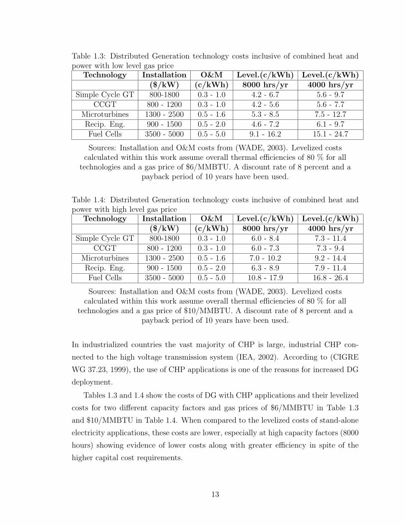
Table 1.3: Distributed Generation technology costs inclusive of combined heat andpower with low level gas price

Technology Installation O&M Level.(c/kWh) Level.(c/kWh)($/kW) (c/kWh) 8000 hrs/yr 4000 hrs/yr

Simple Cycle GT 800-1800 0.3 - 1.0 4.2 - 6.7 5.6 - 9.7CCGT 800 - 1200 0.3 - 1.0 4.2 - 5.6 5.6 - 7.7

Microturbines 1300 - 2500 0.5 - 1.6 5.3 - 8.5 7.5 - 12.7Recip. Eng. 900 - 1500 0.5 - 2.0 4.6 - 7.2 6.1 - 9.7Fuel Cells 3500 - 5000 0.5 - 5.0 9.1 - 16.2 15.1 - 24.7

Sources: Installation and O&M costs from (WADE, 2003). Levelized costscalculated within this work assume overall thermal efficiencies of 80 % for all

technologies and a gas price of $6/MMBTU. A discount rate of 8 percent and apayback period of 10 years have been used.

Table 1.4: Distributed Generation technology costs inclusive of combined heat andpower with high level gas price

Technology Installation O&M Level.(c/kWh) Level.(c/kWh)($/kW) (c/kWh) 8000 hrs/yr 4000 hrs/yr

Simple Cycle GT 800-1800 0.3 - 1.0 6.0 - 8.4 7.3 - 11.4CCGT 800 - 1200 0.3 - 1.0 6.0 - 7.3 7.3 - 9.4

Microturbines 1300 - 2500 0.5 - 1.6 7.0 - 10.2 9.2 - 14.4Recip. Eng. 900 - 1500 0.5 - 2.0 6.3 - 8.9 7.9 - 11.4Fuel Cells 3500 - 5000 0.5 - 5.0 10.8 - 17.9 16.8 - 26.4

Sources: Installation and O&M costs from (WADE, 2003). Levelized costscalculated within this work assume overall thermal efficiencies of 80 % for all

technologies and a gas price of $10/MMBTU. A discount rate of 8 percent and apayback period of 10 years have been used.

In industrialized countries the vast majority of CHP is large, industrial CHP con-

nected to the high voltage transmission system (IEA, 2002). According to (CIGRE

WG 37.23, 1999), the use of CHP applications is one of the reasons for increased DG

deployment.

Tables 1.3 and 1.4 show the costs of DG with CHP applications and their levelized

costs for two different capacity factors and gas prices of $6/MMBTU in Table 1.3

and $10/MMBTU in Table 1.4. When compared to the levelized costs of stand-alone

electricity applications, these costs are lower, especially at high capacity factors (8000

hours) showing evidence of lower costs along with greater efficiency in spite of the

higher capital cost requirements.

13

1.4.2 Impact of DG on reliability (security of supply)

It seems quite clear that the presence of DG tends to increase the level of system

security. To confirm this idea, consider the example in Figure 1.7.

Figure 1.7 shows a very simple distribution network. It consists of two radial

feeders, each with 10 MW of capacity, which feed busbar B. A constant load of 10

MW is connected to B. The forced outage rate (FOR) of the two feeders is given in the

table in Figure 1.7. Additionally, consider a 10 MW DG source with an availability

factor of 80 percent.

To begin with, only consider the two feeders and assume there is no distributed

resource connected to busbar B. The loss of load probability (LOLP), the probability

that load is not served, is simply the probability of both feeders being out of service at

the same time which can be calculated by multiplying the two probabilities of failure.

Consequently, LOLP= (0.04 x 0.04) = 0.0016. The expected number of days in which

the load is not served can also be calculated multiplying the LOLP by 365, which

results in 0.584 days/year. This number can be expressed in hours/year multiplying

by 24, resulting in 14 hours/year.

Now consider including the DG source. It has an outage rate greater than the

two feeders at 0.20, but it also adds a triple redundancy to the system. Thus the

addition of the DG source is expected to decrease the LOLP. The new LOLP is the

probability that both feeders fail and the DG source is not available. Therefore, the

LOLP = (0.04 x 0.04 x 0.20) = 0.00032. That is, the probability of being unable to

serve load is five times less than before. This translates to an expected number of

hours per year unable to serve load at just less than 3 hours per year in this example.

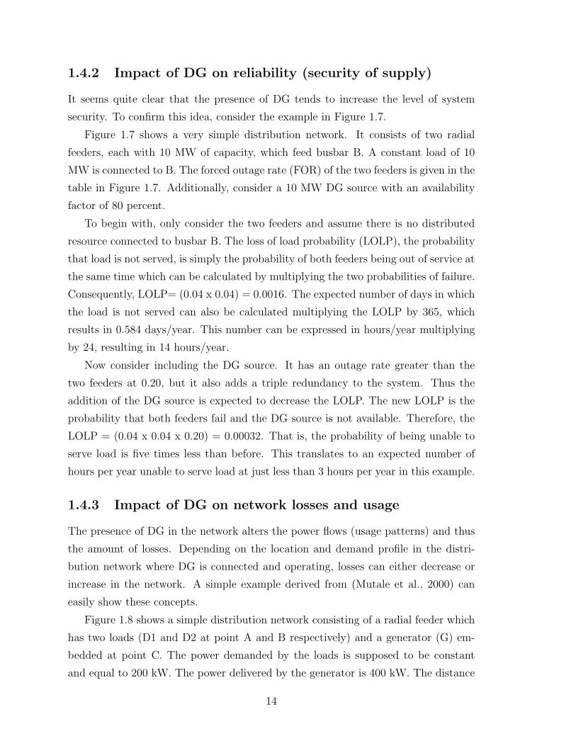
1.4.3 Impact of DG on network losses and usage

The presence of DG in the network alters the power flows (usage patterns) and thus

the amount of losses. Depending on the location and demand profile in the distri-

bution network where DG is connected and operating, losses can either decrease or

increase in the network. A simple example derived from (Mutale et al., 2000) can

easily show these concepts.

Figure 1.8 shows a simple distribution network consisting of a radial feeder which

has two loads (D1 and D2 at point A and B respectively) and a generator (G) em-

bedded at point C. The power demanded by the loads is supposed to be constant

and equal to 200 kW. The power delivered by the generator is 400 kW. The distance

14

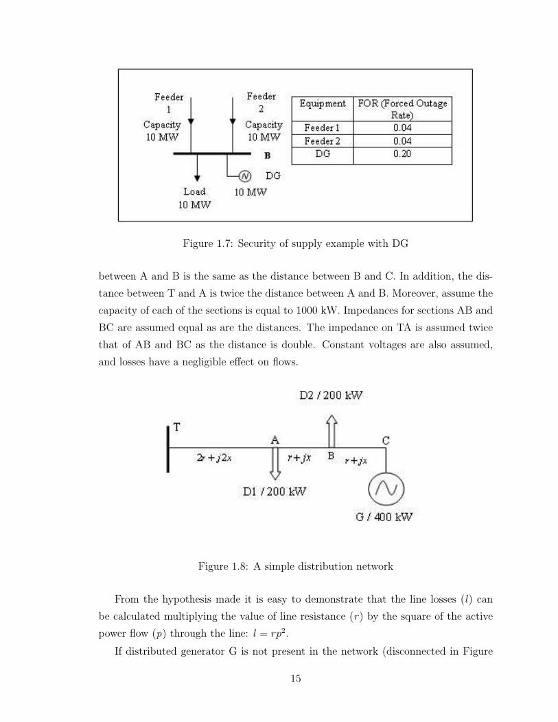
Figure 1.7: Security of supply example with DG

between A and B is the same as the distance between B and C. In addition, the dis-

tance between T and A is twice the distance between A and B. Moreover, assume the

capacity of each of the sections is equal to 1000 kW. Impedances for sections AB and

BC are assumed equal as are the distances. The impedance on TA is assumed twice

that of AB and BC as the distance is double. Constant voltages are also assumed,

and losses have a negligible effect on flows.

Figure 1.8: A simple distribution network

From the hypothesis made it is easy to demonstrate that the line losses (l) can

be calculated multiplying the value of line resistance (r) by the square of the active

power flow (p) through the line: l = rp2.

If distributed generator G is not present in the network (disconnected in Figure

15

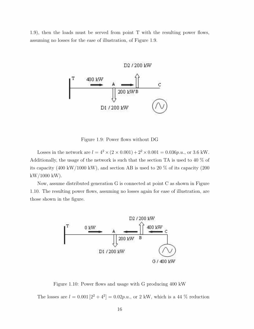
1.9), then the loads must be served from point T with the resulting power flows,

assuming no losses for the ease of illustration, of Figure 1.9.

Figure 1.9: Power flows without DG

Losses in the network are l = 42× (2× 0.001)+22×0.001 = 0.036p.u., or 3.6 kW.

Additionally, the usage of the network is such that the section TA is used to 40 % of

its capacity (400 kW/1000 kW), and section AB is used to 20 % of its capacity (200

kW/1000 kW).

Now, assume distributed generation G is connected at point C as shown in Figure

1.10. The resulting power flows, assuming no losses again for ease of illustration, are

those shown in the figure.

Figure 1.10: Power flows and usage with G producing 400 kW

The losses are l = 0.001 [22 + 42] = 0.02p.u., or 2 kW, which is a 44 % reduction

16

in losses compared to the case without DG. The reduction in losses comes from

transferring flows from the longer circuit TA to a shorter circuit BC. Moreover, since

less power must travel over the transmission network to serve the loads D1 and D2,

losses on the transmission system are reduced, all else equal.

Additionally, the pattern of usage has also changed. The usage on AB is still 200

kW, but the flow is in the opposite direction from the case without DG. The flow

on TA has been reduced from 400 kW to 0 kW. In effect, the DG source at C has

created an additional 400 kW of capacity on TA to serve growing loads at A and B.

For example, suppose the loads D1 and D2 increased to 700 kW each. Without DG,

this would require extra distribution capacity be added over TA, but with DG, no

additional distribution capacity is needed to serve the increased load. In short, DG

has the ability to defer investments in the network if it is sited in the right location.

It is important to emphasize that the potential benefits from DG are contingent

upon patterns of generation and use. For different generation patterns, usage and

losses would be different. In fact, losses may increase in the distribution network as

a result of DG. For example, let G produce 600 kW. For this case, losses are 6 kW,

greater than the 3.6 kW losses without DG. Moreover, while DG effectively creates

additional distribution capacity in one part of the network, it also increases usage in

other parts of the network over circuit BC. In Figure 1.11 shows the curve Losses vs.

Generation. As it can be seen, losses first decrease as DG output increases, reaching

a minimum when generation is 225 kW. After this point, losses begin to increase.

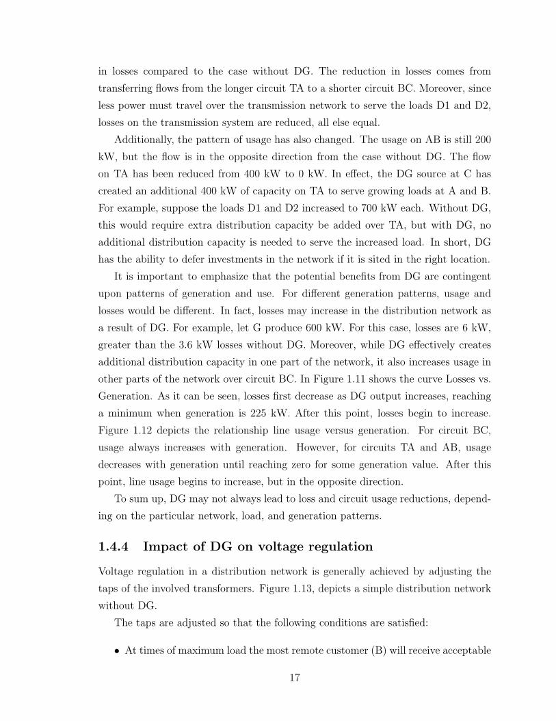
Figure 1.12 depicts the relationship line usage versus generation. For circuit BC,

usage always increases with generation. However, for circuits TA and AB, usage

decreases with generation until reaching zero for some generation value. After this

point, line usage begins to increase, but in the opposite direction.

To sum up, DG may not always lead to loss and circuit usage reductions, depend-

ing on the particular network, load, and generation patterns.

1.4.4 Impact of DG on voltage regulation

Voltage regulation in a distribution network is generally achieved by adjusting the

taps of the involved transformers. Figure 1.13, depicts a simple distribution network

without DG.

The taps are adjusted so that the following conditions are satisfied:

• At times of maximum load the most remote customer (B) will receive acceptable

17

Figure 1.11: Variation of network losses for different DG production

voltage (above the minimum allowed).

• At times of minimum load the customers will receive acceptable voltage (below

the maximum allowed).

If we now consider DG connected to the circuit of Figure 1.13, as indicated in Fig-

ure 1.14, the load flows, and hence the voltage profiles, will change in the distribution

network.

If the generator is exporting, then this will cause the voltage to rise. The degree

of the rise will depend on many factors such as the following:

• Level of export relative to the minimum load on the network

• Siting of the generator (proximity to a busbar where the voltage is regulated by

the distribution company)

• Distribution of load on the network

• Network impedance from busbar to generator

• Type and size of generator

• Magnitude and direction of reactive power flow on the network

18

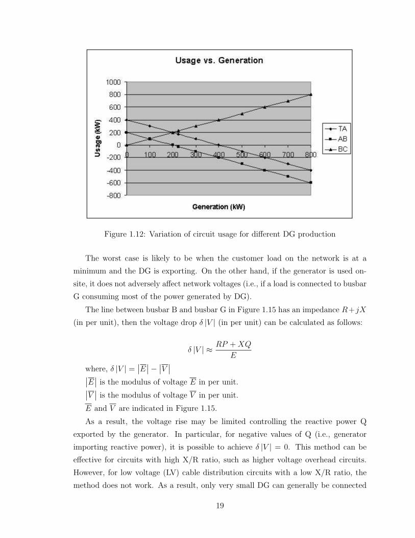
Figure 1.12: Variation of circuit usage for different DG production

The worst case is likely to be when the customer load on the network is at a

minimum and the DG is exporting. On the other hand, if the generator is used on-

site, it does not adversely affect network voltages (i.e., if a load is connected to busbar

G consuming most of the power generated by DG).

The line between busbar B and busbar G in Figure 1.15 has an impedance R+jX

(in per unit), then the voltage drop δ |V | (in per unit) can be calculated as follows:

δ |V | ≈ RP + XQ

E

where, δ |V | =∣∣E

∣∣−∣∣V

∣∣∣∣E

∣∣ is the modulus of voltage E in per unit.∣∣V∣∣ is the modulus of voltage V in per unit.

E and V are indicated in Figure 1.15.

As a result, the voltage rise may be limited controlling the reactive power Q

exported by the generator. In particular, for negative values of Q (i.e., generator

importing reactive power), it is possible to achieve δ |V | = 0. This method can be

effective for circuits with high X/R ratio, such as higher voltage overhead circuits.

However, for low voltage (LV) cable distribution circuits with a low X/R ratio, the

method does not work. As a result, only very small DG can generally be connected

19

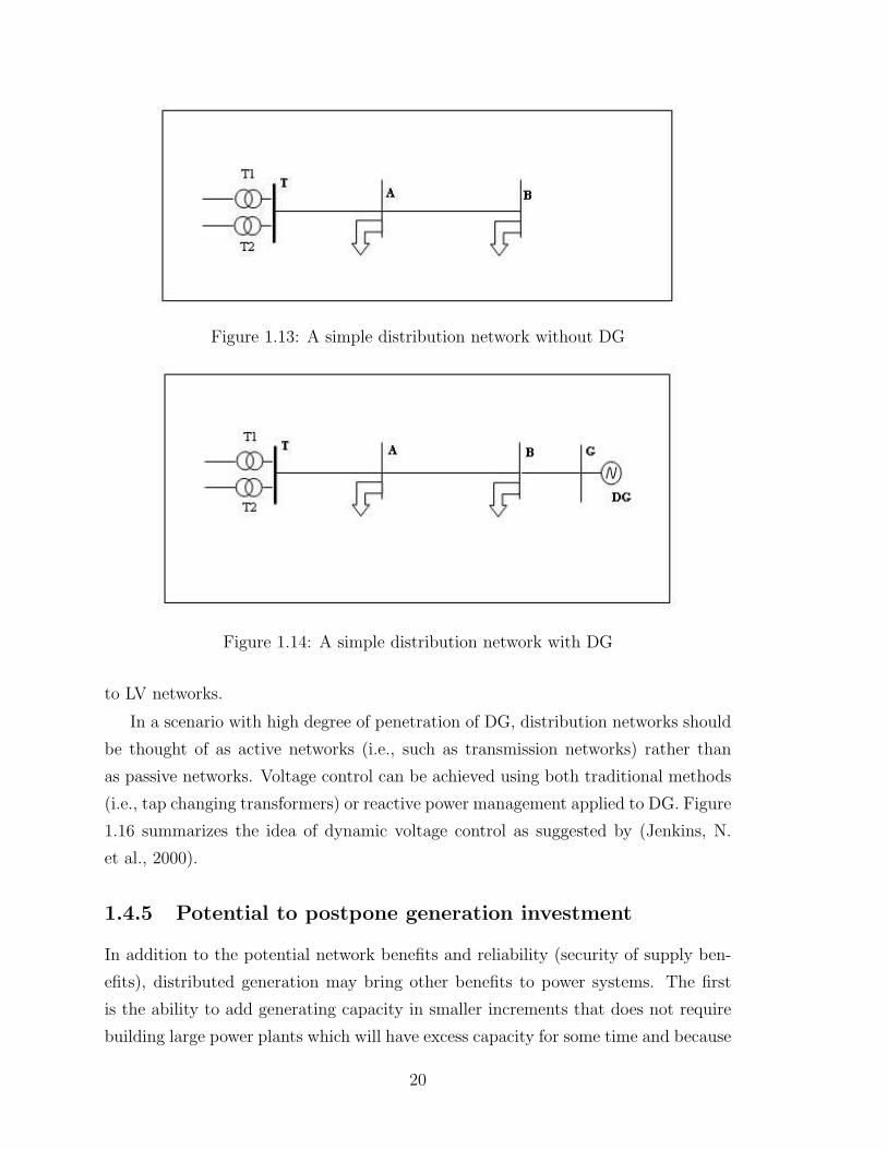
Figure 1.13: A simple distribution network without DG

Figure 1.14: A simple distribution network with DG

to LV networks.

In a scenario with high degree of penetration of DG, distribution networks should

be thought of as active networks (i.e., such as transmission networks) rather than

as passive networks. Voltage control can be achieved using both traditional methods

(i.e., tap changing transformers) or reactive power management applied to DG. Figure

1.16 summarizes the idea of dynamic voltage control as suggested by (Jenkins, N.

et al., 2000).

1.4.5 Potential to postpone generation investment

In addition to the potential network benefits and reliability (security of supply ben-

efits), distributed generation may bring other benefits to power systems. The first

is the ability to add generating capacity in smaller increments that does not require

building large power plants which will have excess capacity for some time and because

20

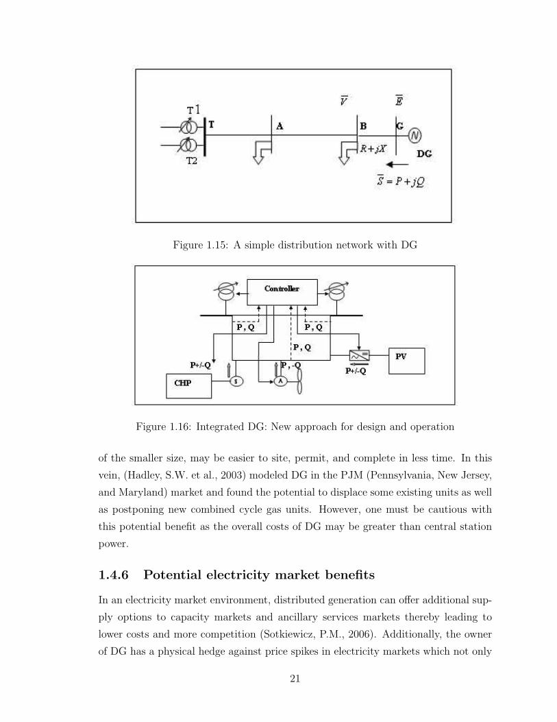
Figure 1.15: A simple distribution network with DG

Figure 1.16: Integrated DG: New approach for design and operation

of the smaller size, may be easier to site, permit, and complete in less time. In this

vein, (Hadley, S.W. et al., 2003) modeled DG in the PJM (Pennsylvania, New Jersey,

and Maryland) market and found the potential to displace some existing units as well

as postponing new combined cycle gas units. However, one must be cautious with

this potential benefit as the overall costs of DG may be greater than central station

power.

1.4.6 Potential electricity market benefits

In an electricity market environment, distributed generation can offer additional sup-

ply options to capacity markets and ancillary services markets thereby leading to

lower costs and more competition (Sotkiewicz, P.M., 2006). Additionally, the owner

of DG has a physical hedge against price spikes in electricity markets which not only

21

benefits the owner of DG, but should also help dampen the price volatility in the

market (IEA, 2002).

1.4.7 Potential environmental benefits

Finally, distributed generation resources may have lower emissions than traditional

fossil-fired power plants for the same level of generation as can be observed in Table

1.2, depending on technology and fuel source. Of course, this is true for renewable

DG technologies. The benefits are potentially large in systems where coal dominates

electricity generation as can also be seen in Table 1.2. (Hadley, S.W. et al., 2003)

model DG in the PJM market and find DG displacing generation on the system led

to lower emissions levels. (CIGRE WG 37.23, 1999) cited these reasons as determin-

ing factors for some DG deployment. Moreover, since losses may also be reduced,

distributed generation may reduce emissions from traditional generation sources as

well. Additionally, increased customer demand for renewable energy because of its

lower emissions profile may also be a factor be driving renewable energy deployment

(Hyde, D., 1998).

1.5 Policies and Chapter Concluding Remarks

Though it is not yet competitive with grid-supplied power on its own, distributed

generation can provide many benefits. Current policies to induce DG additions to the

system generally consist of tax credits and favorable pricing for DG-provided energy

and services that are subsidized by government (IEA, 2002). While such policies

may be effective to capture some potential benefits from DG, such as environmental

benefits, they do not address the network or market benefits of DG, as it will be

discussed in next chapter.

This dissertation will consider locational pricing of network services as a way to

provide better incentives without subsidies as recommended by (IEA, 2002). A new

tariff scheme is proposed for distribution networks with DG, which uses nodal prices

to recover losses and an “extent-of-use” method to recover fixed network costs.

22

Chapter 2

Current Schemes for DistributionPricing

2.1 Costs in the Distribution Business

The distribution business consists of the transportation of electricity from the points

of transmission supply at high voltages (power supply points or PSPs) to the end-

use consumers. Within the new electricity industry model (i.e., after restructuring)

a distinction is made between “distribution” and “supply” of electricity (Williams,

P. and Strbac, G., 2001). “Distribution” refers only to the wires business or the

network service, while “supply” is related to the commercialization of the “electricity

product”. Although in some countries like the UK, there is actually retail competition

with different companies doing “distribution” and “supply” at the same location, in

the majority of the other cases worldwide, the same company is engaged in both

businesses as a single distribution service.

The distribution of electricity basically involves two types of costs: capital costs

and operational costs.

2.1.1 Capital costs

The capital costs refer both to the ongoing expenditures in new assets, as well as the

cost of capital for all the installed assets owned by the distribution company, which

need to be paid an expected rate of return.

In those countries where a restructured electricity industry model applies, the

regulator establishes a value of the asset base (i.e., regulatory value of the existing

assets) as well as a rate of return, which must be applied to assure an adequate

capital remuneration. In addition, some kind of depreciation rule for the asset base

23

is generally defined to allow for depreciation charges.

Different methodologies are applied to evaluate the asset base. In (Foster, V. and

Antmann, P., 2004) these methodologies are divided into two categories: economic

value or market-based and replacement-cost-based.

The economic value is the value that the market offers for the distribution business

in the service area, and it is related to the capacity of the assets to generate profits.

For instance, it can be the price resulting from a public auction in a privatization

process of a distribution company. In this case, once the allowed tariffs are determined

by the regulator or government for the distribution company, it is possible to calculate

the net present value of the assets. However, if tariffs are not determined in advance,

the privatization price cannot be used to determine the asset value for future tariff

setting purposes due to a circularity problem in that the asset value is dependant on

the future tariff level which is itself dependant on the asset value.

On the other hand, the replacement-cost-based methodologies imply a cost eval-

uation of the distribution assets. This cost evaluation can be done in different man-

ners. One possibility is to use the current cost valuation (CCV) method, which uses

historic purchase prices adjusting them through inflation and depreciation over the

corresponding period. A variation of the CCV is the use of historic accounting costs,

which uses historic purchase prices and adjusts them only through depreciation over

the period (i.e., inflation is not taken into account) (Bernstein, J.S., 1999). Another

way is to use the depreciated optimized replacement cost (DORC), which evaluates

the replacement cost of each individual asset at current purchase prices and then

adjusts the value for depreciation taking into account the asset age. Finally, a third

method within cost replacement is the reference utility or gross optimized replacement

cost (GORC) methodology, which supposes the creation of a hypothetical distribution

company that provides the same service as the regulated one but in an efficient man-

ner. Then the present purchasing costs of the reference utility assets are evaluated to

determine the asset base.

As discussed in (Foster, V. and Antmann, P., 2004), there is not a universally

accepted methodology for asset valuation. All the described methodologies have

been used by regulators worldwide. For instance, economic valuation has been used

in the UK. In Australia, regulators have been increasingly opting for DORC, while in

several countries in Latin America the GORC (reference utility) has been used. For

the same case, different methodologies could give result discrepancies of 2:1 or more,

24

which normally lead to opposite positions between regulators and companies, as it is

shown in detail for the Brazilian case by (Foster, V. and Antmann, P., 2004).

2.1.2 Operational costs

The operational costs are the costs incurred by the distribution company to run the

business. These costs include technical and administrative employee wages, office

and land rent, transportation and fuel costs, metering and billing, operation and

maintenance (O,&M) costs of lines, cables, transformers, circuit breakers, and other

equipment.

Important components of the operation costs are the losses, both technical and

nontechnical. Technical losses refer to the Joule losses in lines, cables, and transform-

ers, which depend mainly on the equipment capacity (e.g., cross-sectional area in lines

and cables), voltage level, and actual current flow. On the other hand, nontechnical

losses include electricity theft and mistakes in measurement and billing. 1

2.1.3 Fixed and variable costs

For the purpose of this work, distribution costs will be grouped into fixed costs and

variable costs.

Fixed costs are the costs that do not change with throughput in the short run.

These costs include all capital costs plus the nonvariable operational costs.

On the other hand, variable costs are those which change with throughput. Apart

from technical losses, which actually change with power flow patterns, there is gen-

erally little if any other variable operational costs. As a result, technical losses are

assumed to be the only variable costs.

2.2 Traditional Cost Allocation Methodologies

Traditionally, distribution costs have typically been allocated on a pro rata basis either

using a volumetric (per MWh) charge and/or a fixed charge based on kW demand at

either coincident or noncoincident peak. The cost-allocation methods translate into

two basic tariff setting methods. The first tariff method consists of full averaging of

all distribution costs, fixed and variable, into a single per MWh charge. The second

tariff method consists of averaging losses plus some portion of other distribution costs

1Only technical losses are considered within this work.

25

into a MWh charge, and taking the remaining distribution costs and allocating them

through fixed charges based on kW demand at coincident or noncoincident peak.

The reason for using these simple, traditional methods for allocating distribu-

tion costs is that the cost of service for areas of similar density parameters (e.g.,

number of customers per km or kWh per inhabitant) tend to be similar. As a re-

sult, current practices assess the distribution costs dividing the whole service area

of the distribution company in areas with different density parameters. Each area

has an assigned cost to be recovered through the distribution tariffs (for instance, in

Chile this cost is expressed in $/kW, while in England and Colombia it is expressed

in $/kWh, (Bernstein, J.S., 1999)). Total distribution area costs are then used to

calculate tariffs.

The following variables are defined to mathematically characterize the expressions

describing the traditional cost allocation methodologies:

k is the index of busses on the distribution network with k = 0, ..., n.

k = 0 is the reference bus, and this is also the power supply point (PSP) for the

distribution network.

t is the time index with t = 1, ..., T .

Subscripts d and g represent demand and generation.

Pdtk and Pgtk are the active power withdrawals by demand and injections by genera-

tion respectively at node k at time t.

λt is the price of power at the reference bus at time t.

Losst is the line loss at time t.

l is the index of circuits with l = 1, ..., L.

CCl accounts for all fixed costs of circuit l.

peak is a superscript denoting values at the coincident peak.

2.2.1 Average losses

Averaging losses over all MWh sold is a traditional allocation scheme used in many

countries, though it does not provide either locational or time-of-use signals to net-

work users. The tariff charge related to losses to customer d at node k over all time

periods is obtained simply by dividing the loss cost by the total active energy con-

sumed in the network, and multiplying by the customer’s consumption as defined in

equation 2.2.1.

26

ALdk =

∑Tt=1 Pdtk∑T

t=1

∑nk=1 Pdtk

T∑t=1

Losstλt (2.2.1)

It is important to note in equation 2.2.1 losses are allocated to only demand

customers and not to DG. This is the practice followed in Uruguay for DG sources

connected to the system (Decreto PE No277/02 Uruguay, 2002). This rule is a sim-

plistic attempt by the regulator to recognize the potential benefits of DG in reducing

line losses.2

However, DG connected at bus k still collects revenue from selling power and is

paid the prices at the PSP, λt each period it runs.

RALgk =

T∑t=1

Pgtkλt (2.2.2)

2.2.2 Allocation of fixed costs

Per MWh average charges

The per MWh charge is computed by dividing the total fixed costs of all circuits by

the total active energy consumed in the network regardless of time or location and,

therefore, does not provide incentives to customers to reduce the use of potentially

congested or congestible network infrastructure. The total charges for customer d at

node k over all time periods t is

NACdk =

∑Tt=1 Pdtk∑T

t=1

∑nk=1 Pdtk

L∑

l=1

CCl. (2.2.3)

Once again, following the regulatory practice in Uruguay, distributed generation

resources do not face fixed network charges.

Coincident peak charges

The network costs are divided by the yearly system peak load (in MW), and the

charges are allocated to the customers according to their contribution to that peak

(i.e., coincident peak); a fixed charge per year is obtained. Note that if a particular

2However, as seen in the previous chapter, DG may either reduce or increase losses in the distri-bution network.

27

customer has zero consumption at the yearly system peak load, then the charge will

be zero.

This allocation method provides a time-of-use signal insofar as it encourages

smoother consumption or a higher load factor, but still does not provide a locational

price signal. The charge for customer d at node k is

NPCdk =P peak

dk∑nk=1 P peak

dk

L∑

l=1

CCl. (2.2.4)

It is assumed here that distributed generation does not face fixed network charges

under this tariff scheme as would be regulatory practice in Uruguay.

2.2.3 Full charges

The full charge for a given demand customer d at node k is obtained by adding the

charge related to losses and the charge related to fixed costs. According to the two

basic tariff setting methods explained before, two possibilities arise: full average cost

(FAC), which results from the summation of 2.2.1 and 2.2.3 according to equation

2.2.5; or averaging losses plus a fixed charge for fixed costs (ALFC) which results

from the summation of 2.2.1 and 2.2.4 according to equation 2.2.6.

FACdk =

∑Tt=1 Pdtk∑T

t=1

∑nk=1 Pdtk

(T∑

t=1

Losstλt +L∑

l=1

CCl) (2.2.5)

ALFCdk =

∑Tt=1 Pdtk∑T

t=1

∑nk=1 Pdtk

T∑t=1

Losstλt +P peak

dk∑nk=1 P peak

dk

L∑

l=1

CCl (2.2.6)

2.2.4 The effect of traditional cost allocation methodologieson the development of DG

As can be observed, these traditional cost allocation and tariff methodologies likely

do not provide adequate incentives for the deployment of DG as no consideration is

given to DG resources that may reduce network use or losses.

Although simple, averaging costs over typical distribution areas does not deter-

mine the impact of each customer on each network asset based on location or time.

28

Within this approach, all customers with the same levels of consumption or peak de-

mand are assumed to be equally responsible for the costs and thus must pay for them.

In contrast to the per MWh average charges, coincident peak charges send a time-

of-use signal encouraging higher load factor in the system. Higher load factors may

benefit the network in term of reduced use at peak and losses over the year. However,

with none of these methods, a distinction is made between a demand customer sited

at the end of a very long line, which may have a great impact increasing network use

and losses, with others sited near the main distribution substation, which may im-

pose lower network use or losses. In the same way, the impact of a DG resource will

be different dependent on location. Consequently the tariff scheme applied should

properly recognize this.

2.3 Present Pricing and Policy Approaches with

respect to DG

Looking at different regulatory frameworks worldwide, what can be observed is that

DG faces distribution pricing schemes that were developed for loads and not for gener-

ation. In the most favorable cases, DG is exempted from all or part of the distribution

network charges that all other demand customers must pay to the distribution com-

pany. These policies attempt to recognize the potential benefits of DG, for instance,

in reducing network use and losses. However, they can lead to inefficiencies and poor

incentives because, as seen in the previous chapter DG can, in some cases, increase

network use or losses.

Examples of these types of pricing schemes can be observed in the Netherlands

and in Uruguay. In the case of the Netherlands, small DG under 10 MVA is exempted

from all the distribution network charges. However, DG above 10 MVA pays both

distribution use of system charges and full connection charges (IEA, 2002). In the

case of Uruguay, DG 3 is released from the distribution use of system charges, but

must pay deep connection charges (i.e., all reinforcement costs in the network due to

DG connection) (Decreto PE No277/02 Uruguay, 2002).

Only recently, efforts can be seen in the direction of creating new tariff frame-

works that consider the presence of DG in the distribution network and its specific

nature. This is the case in the UK, where OFGEM has been implementing new tariff

3Under the Uruguayan regulatory framework, DG is the generation connected to the distributionnetwork with an installed capacity not greater than 5 MW.

29

arrangements for DG (OFGEM, 2005). In the UK, DG paid deep connection charges

until April 2005 when the regulations changed to a shallow connection charge plus a

distribution use of system charges scheme (OFGEM, 2005).

Rather than considering DG pricing as a distribution network pricing problem,

most countries which are aware of the potential benefits of DG adopt specific ad-hoc

policies such as subsidies, tax credits, etc., or exempt DG from charges, as seen before,

which is a form of a subsidy (IEA, 2002).

For example, in Japan, CHP benefits from investment incentives such as tax

credits, low interest rate loans and investment subsidies. In the Netherlands, CHP

has benefited from investment subsidies and favorable natural gas prices; at present,

CHP benefits from tax credits, exemption of CHP electricity consumption from the

regulatory energy tax, and financial support of EUR 2.28/MWh (for output up to

200 GWh) (IEA, 2002). Similar policies can be seen in other countries worldwide

(WADE, 2006).

2.4 Chapter Concluding Remarks

The presence of DG in the distribution network transforms distribution from a passive

network (e.g., a network that only has loads connected to it) into an active network,

not unlike a transmission network. Traditional cost allocation methods do not rec-

ognize this, and as a result other policies such as subsidies and tax credits have been

used to induce greater penetration of DG. As an alternative to the use of subsidies

and tax credits, cost-allocation methodologies used for transmission networks such as

nodal pricing (extensively used in various forms by electricity markets in New York,

New England, PJM, Argentina, and Chile) and MW-mile (which has been used for

instance in the UK, Argentina, and Uruguay) could be adopted to promote more

cost-reflective pricing at the distribution level, which will provide better financial

incentives for the entry and location of DG or large loads on, and investment in,

distribution networks. Following this idea, the next chapter assesses nodal pricing

and a usage-based allocation methodology applied to the distribution network.

30

Chapter 3

A New Distribution TariffFramework for Efficient EnhancingDG 1

3.1 Nodal Pricing for Distribution Networks

As distributed generation (DG) becomes more widely deployed in distribution net-

works, distribution takes on many of the same characteristics as transmission in that it

becomes more active rather than passive. Consequently, pricing mechanisms that have

been employed in transmission, such as nodal pricing as first proposed in (Schweppe

et al., 1988), are good candidates for use in distribution. Nodal pricing is an economi-

cally efficient pricing mechanism for short-term operation of transmission systems and

has been implemented in various forms by electricity markets in New York, New Eng-

land, PJM, New Zealand, Argentina, and Chile. Clearly, this is a pricing mechanism

with which there is a great deal of experience and confidence.

While nodal pricing is most often associated with pricing congestion as discussed in

(Hogan, W.W., 1998), the pricing of line losses at the margin, which can be substantial

in distribution systems with long lines and lower voltages, can be equally important.

In this section, the use of nodal pricing in distribution networks is proposed. Nodal

pricing sends the right price signals to locate DG resources, and to properly reward

DG resources for reducing line losses through increased revenues derived from prices

that reflect marginal costs.

The manner in which nodal prices are derived in a distribution network is no

1This chapter draws heavily in both text and concept from the published versionsof (Sotkiewicz, P.M. and Vignolo, J.M. 1/06, 2006) and (Sotkiewicz, P.M. and Vignolo,J.M. 2/06, 2006).

31

different from deriving them for an entire power system. Let t, k, g, and d be the

indices of time, busses, generators at each bus k, and loads at each bus k. Define

Pgk, Qgk and Pdk, Qdk respectively, as the active and reactive power injections and

withdrawals by generator g or load d located at bus k. The interface between gener-

ation and transmission, the power supply point (PSP), is treated as a bus with only

a generator. P and Q without subscripts represent the active and reactive power

matrices respectively.

Let Cgk(Pgk, Qgk) be the total cost of producing active and reactive power by

generator g at bus k where Cgk is assumed to be convex, weakly increasing, and once

continuously differentiable in both of its arguments. The loss function Loss(P,Q)

is convex, increasing, and once continuously differentiable in all of its arguments. I

assume no congestion on the distribution network and that the generator prime mover

and thermal constraints are not binding.

The optimization problem for dispatching distributed generation and power from

the PSP can be represented as the following least-cost dispatch problem at each time

t:

minPgtk,Qgtk∀gk,dk

∑

k

∑g

Cgk(Pgtk, Qgtk) (3.1.1)

subject to

Loss(P,Q)−∑

k

∑g

Pgtk +∑

k

∑

d

Pdtk = 0,∀t (3.1.2)

Application of the Karush-Kuhn-Tucker conditions lead to a system of equations

and inequalities that guarantee the global maximum (Nemhauser et al., 1989).

The net withdrawal position for active and reactive power at each bus k at time

t are defined by Ptk =∑

d Pdtk −∑

g Pgtk and Qtk =∑

d Qdtk −∑

g Qgtk. Nodal

prices are calculated using power flows locating the “reference bus” at the PSP, so

λt corresponds to the active power price at the PSP. Assuming interior solutions, the

following prices for active and reactive power respectively are as follows:

patk = λt(1 +∂Loss

∂Ptk

) (3.1.3)

prtk = λt(∂Loss

∂Qtk

) (3.1.4)

32

3.1.1 Full marginal losses from nodal prices

The charge for marginal losses for loads at bus k summed over all time periods t is

MLdk =T∑

t=1

λt[(∂Losst

∂Ptk

)Pdtk + (∂Losst

∂Qtk

)Qdtk]. (3.1.5)

Under nodal pricing, distributed generation connected to the network is paid the

nodal price including marginal losses. The revenue collected by distributed generation

at bus k summed over all time periods t is

RMLgk =

T∑t=1

λt[(1 +∂Losst

∂Ptk

)Pgtk + (∂Losst

∂Qtk

)Qgtk]. (3.1.6)

The distribution company recovers energy costs inclusive of losses plus a merchan-

dising surplus over all hours t (MS ) equal to

MS =T∑

t=1

n∑

k=1

[patk(Pdtk − Pgtk) + prtk(Qdtk −Qgtk)]

−T∑

t=1

λtPt0 (3.1.7)

MS =T∑

t=1

n∑

k=1

λt[(1 +∂Losst

∂Ptk

)(Pdtk − Pgtk)

+(∂Losst

∂Qtk

)(Qdtk −Qgtk)]−T∑

t=1

λtPt0. (3.1.8)

It should be noted that, in general, the merchandising surplus is greater than

zero, which means that the total amount paid by demand customers in the distri-

bution network is greater than the whole sum paid to generators. This leads to an

overcollection of losses.

In the case of transmission, it has been argued that the MS should not be used to

finance the network company because of the high volatility, the perverse short-term

incentives to increase losses, and the insufficiency of the MS to cover all network costs

(Bialek, J. 1/97, 1997). However, as it will be seen later in this chapter, the yearly

MS can be used to offset the fixed distribution costs, without the poor short-term

effects mentioned above.

33

3.1.2 Reconciliated marginal losses

As suggested by (Mutale et al., 2000), it may be desirable for other reasons not to

overcollect for losses as would be the case under nodal prices. (Mutale et al., 2000)

suggests adjusting marginal loss coefficients so that the nodal prices derived collect

exactly the cost of losses. This method can be called reconciliated marginal losses.

One particular reconciliation method is offered below. The approximation of losses

in the distribution network, ALosst is defined as

ALosst =n∑

k=1

(∂Loss

∂Ptk

Ptk +∂Loss

∂Qtk

Qtk). (3.1.9)

Dividing the actual losses by the approximation of losses provides the reconcilia-

tion factor in period t, RFt.

RFt =Losst

ALosst

(3.1.10)

Reconciliated prices can then be computed, similar to the prices in equations

(3.1.3) and (3.1.4), but with the marginal loss factors multiplied by the reconciliation

factor and the resulting loss charges for load summed over all time periods t for bus

k.

partk = λt(1 + RFt

∂Losst

∂Ptk

) (3.1.11)

prrtk = λt(RFt

∂Losst

∂Qtk

) (3.1.12)

RLdk =T∑

t=1

λtRFt(∂Losst

∂Ptk

Pdtk +∂Losst

∂Qtk

Qdtk) (3.1.13)

Under reconciliated nodal pricing distributed generation connected to the network

is paid the nodal price including marginal losses. The revenue collected by DG at bus

k summed over all time periods t is

RRLgk =

T∑t=1

(λtPgtk + λtRFt[(∂Losst

∂Ptk

)Pgtk

+(∂Losst

∂Qtk

)Qgtk]). (3.1.14)

34

The resulting reconciliated merchandising surplus is equal to zero by construction.

This method overcomes the concerns regarding the overcollection of losses men-

tioned previously, although it dampens the signals and reduces the efficiency proper-

ties of nodal pricing.

MSr =T∑

t=1

n∑

k=1

[partk(Pdtk − Pgtk) + prr

tk(Qdtk −Qgtk)]

−T∑

t=1

λtPt0 (3.1.15)

MSr =T∑

t=1

n∑

k=1

λt[(1 + RFt∂Losst

∂Ptk

)(Pdtk − Pgtk)

+RFt(∂Losst

∂Qtk

)(Qdtk −Qgtk)]−T∑

t=1

λtPt0

=T∑

t=1

n∑

k=1

λt(Pdtk − Pgtk + Losst)−T∑

t=1

λtPt0 = 0 (3.1.16)

3.2 Allocation of Fixed Costs: The Amp-mile Method-

ology

3.2.1 Extent-of-use methods for distribution networks

It is already well understood that nodal energy prices as developed by (Schweppe

et al., 1988) send short-run efficient time and location differentiated price signals to

load and generation in transmission networks as discussed in (Hogan, W.W., 1998).

These signals can also be used for sending the appropriate signals for the siting of DG

in distribution networks as demonstrated in the last section. While these short-run

efficient nodal prices collect more revenue from loads than is paid out to generators,

it has been shown in (Perez-Arriaga et al., 1995), (Rudnick et al., 1995), and (Pereira

da Silva et al., 2001) to be insufficient to cover the remaining infrastructure and other

fixed costs of the network.

As discussed in Chapter 2, it is also well established that passing through the

remaining infrastructure costs on a pro rata basis, as is often the case in many tariff

methodologies, does not provide price signals that are based on cost causality (cost

reflective), provide for efficient investment in new network infrastructure, or long-term

signals for the location of new loads or generation. Beginning with (Shirmohammadi

35

et al., 1989), many have written about “extent-of-use” methods for the allocation

of transmission network fixed costs. These “extent-of-use” methods for allocating

costs have also become known generically as MW-mile methods as they were called

in (Shirmohammadi et al., 1989). The “extent-of-use” can be generically defined as a

load’s or generator’s impact on a transmission asset (line, transformer, etc. ) relative

to total flows or total capacity on the asset as determined by a load flow model.

Other variations on this same idea can be seen in (Maranagon Lima, J.W., 1996).

An interesting trend in the literature on MW-mile methodologies emerges on closer

examination. As different methods are proposed to allocate fixed transmission costs,

rarely is there any incentive to provide for counter-flow on a transmission asset as

transmission owners worry they would be unable to collect sufficient revenues due

to payments made to generators that provided counter-flows (Shirmohammadi et al.,

1989), (Maranagon Lima et al., 1996), (Kovacs, R.R. and Leverett, A.L., 1994), and

(Pan et al., 2000). (Maranagon Lima et al., 1996) propose recognizing counter-flows,

but to ease potential worries to transmission owners, propose that counter-flows be

assessed a charge of zero.

As there are many cost-allocation methods, there are many load Flow-based meth-

ods to determine the extent-of-use. (Bialek, J. 2/97, 1997), (Bialek, J., 1998), and

(Su, C.T. and Liaw, J.H., 2001) use a tracing method that relies on the use of propor-

tional sharing of flows into and out of any node. Marginal factors such as distribution

factors are used in (Shirmohammadi et al., 1989) and (Rudnick et al., 1995), while

(Park et al., 1998) use line utilization factors that depend on demand in the system

being fixed. (Pan et al., 2000) provide an overview and comparison of these methods

and shows all methods examined arrive at very similar results for flows and charges,

leading to the conclusion that there still is no agreement on the best method to

determine the extent-of-use.

As discussed before, the rationale for examining extent-of-use methods is that the

presence of DG in the distribution network transforms distribution from a passive

network (e.g., a network that only has loads connected to it) into an active network,

not unlike a transmission network. As with nodal pricing for short-run operation

of power systems where price signals are sent so that generators close to loads are

rewarded for reducing losses, or generators locating downstream of a congested as-

set are rewarded for alleviating that congestion, generators or loads that locate in a

manner that reduces line loading or uses fewer assets should be rewarded with lower

36

charges for the recovery of fixed costs as essentially these generators or loads “create”

additional distribution capacity. As a result, extent-of-use, cost- allocation method-

ologies from transmission networks could, and should, be adopted to promote more

cost-reflective pricing which will provide better financial incentives for the entry and

location of DG or large loads on, and investment in, distribution networks.

The extent-of-use measure proposed in this dissertation uses marginal changes

in current, as opposed to power, in a distribution asset with respect to both active

and reactive power injections multiplied by those injections to determine the extent-

of-use at any time t.2 Unlike most previous applications of extent-of-use measures,

this extent-of-use measure explicitly accounts for flow direction to provide better

long-term price signals and incentives for DG to locate optimally in the distribution

network and to alleviate potential constraints and reduce losses.

Two possibilities to price the extent-of-use are proposed, the merits of which will

be discussed in the next section below. First, the extent-of-use can be computed at

each bus in each hour and prices the extent-of-use on a per MWh basis at each bus

in each hour, with any remaining fixed costs spread over all load in the system on a

per MWh basis. The other pricing option explored is the use of fixed charges based

on the extent-of-use at each bus at the system coincident peak, with any remaining

fixed costs recovered over all load at coincident peak.

3.2.2 The Amp-mile methodology: Allocation strategy anddescription of charges

From an economic perspective, allocation methods for fixed costs do not have effi-

ciency properties per se. But the allocation of costs, regardless of the method, is

entirely necessary for the owners of distribution infrastructure, so they may recover

the costs associated with providing distribution service. Thus, given the general lack

of efficiency properties and the need to allocate fixed costs, allocating costs to those

who cause them (cost causality) is another method that is often used, and is the cri-

teria used in the proposed allocation strategy. Moreover, since these are fixed costs

that are being allocated, there are no “short-term” incentive changes that one would

observe akin to the changes that occur when moving to efficient nodal prices for

energy.

2The extent-of-use measure proposed is not a marginal methodology like the nodal pricing of con-gestion and losses, but is analogous to the expenditures incurred or revenues gained (price multipliedby quantity) under nodal pricing.

37

However, long-term entry and siting incentives may change depending on the

allocation of fixed costs. Consider the siting of DG on a distribution system, and

consider an allocation of costs based on the line loading attributable to DG that pays

generators for providing counter-flow that effectively “creates” additional capacity.

This provides a better financial incentive for DG to locate where it provides counter-

flow, versus locating where it increases line loading. In contrast, allocation of costs

based on the extent-of-use will lead a large industrial customer to site its facility closer

to the interface with the transmission system rather than at the end of the network

where line loading will increase for more distribution facilities.

In the design of the proposed allocation strategy, two observations can be made

regarding distribution networks. The first is that distribution networks are designed

primarily to handle circuit currents. The second observation is that current flow bet-

ter corresponds to the thermal capacity limits of a line or asset since voltages may

not necessarily be held constant in the network (Baldick, R., 2003). Consequently,

the “extent-of-use” of distribution network circuits should be measured in terms of

the contribution of each customer to the current flow, not to the power flow, through

the circuit at any point in time similar to (Chu et al., 2001) in their derivation of

utilization factors. This current flow can be traced to injections and withdrawals of

active and reactive power at each busbar using active and reactive power to current

distribution factors, APIDFs and RPIDFs respectively. The proposed extent-of-use

measure is grounded in the idea that costs should be allocated to those who cause

them. Given that it is propose current flows attributed to network customers be

used, this methodology is called the “Amp-mile” or “I-mile” methodology for allocat-

ing fixed distribution network costs. The remainder of this subsection conceptually

describes the methodology, while the mathematical expressions are derived in the

next subsection.

The contribution of a given customer to the current flow on a given circuit at any

time is the summation of the correspondent APIDF and RPIDF multiplied by the

actual active and reactive power respectively injected or withdrawn by the customer

at that time. The summation for a given circuit of all customers’ contributions

closely approximates the current flow. A reconciliation factor must be used to obtain

the exact current flow through the circuit using the APIDFs and the RPIDFs. The

reconciliated contributions can be used as a measure of the “extent-of-use”, and active

power extent-of-use (AEoU) and reactive power extent-of-use (REoU) factors can be

38

obtained.

The fixed cost of each circuit is calculated summing up the capital and nonvariable

operational costs of the conductor and other circuit-related equipment such as circuit

breakers, isolators, dischargers, etc., including installation costs. The capital portion

of the fixed cost is assumed to be a levelized cost. A locational charge for each

customer, which recovers the used network capacity, can be determined summing up

the individual facility charges for circuit usage. These individual charges are obtained

multiplying the correspondent AEoU and REoU factors by the adapted circuit cost

(ACC). The ACC for a circuit is calculated multiplying the levelized circuit cost by the

used circuit capacity (UCC) factor, which is given by the ratio between current flow

and current capacity of the circuit. As suggested by (Maranagon Lima, J.W., 1996)

and (Pan et al., 2000), and employed by (Bialek, J., 1998), any remaining network

costs related to the unused capacity of the circuits can be recovered by a nonlocational

charge.

Each customer (generator/demand) faces two types of charges for the recovery of

fixed costs for the distribution network: a locational charge based on the extent-of-use

and a nonlocational charge covering all other remaining costs that are either averaged

over all MWh or allocated based on contributions to the system coincident peak.

The locational charge considers both active power (active locational charge) and

reactive power (reactive locational charge) injections or withdrawals. Unlike previous

applications of flow-based, extent-of-use methodologies and charges that only account

for flow magnitudes and not flow direction, in the Amp-mile method counter-flows are

explicitly accounted and the method rewards potential DG units that free up or, in ef-

fect, create additional distribution network capacity with negative locational payments

(payments to the DG source). The nonlocational charge is levied to recover the cost

of the unused network capacity and spreads the cost of the unused capacity over all

load in some fashion.3 It can be argued that the spare capacity is a common “sys-

tem benefit” to all users as the excess capacity reduces losses for every customer and

provides system security and, therefore, should be paid for by all users.

There exists a variety of possibilities for assessing the locational and nonlocational

charges. One possibility is to allocate both charges on a per MWh basis. However,

a drawback to allocating charges for fixed costs on a per MWh basis is that it would

3Nonlocational charges are allocated only over load as this is the allocation concept used inUruguay, upon which the forthcoming examples are based. If some costs are allocated to generators,it does not change the results qualitatively.

39

distort short-term price signals if those short-term signals were based on efficient

nodal prices. However, assessing the charges on a per MWh basis would make it

easier to implement the suggestion by (Perez-Arriaga, I.J. and Smeers, Y., 2003) that

extent-of-use charges for network infrastructure may be more long-term efficient if

they are time differentiated to account for different usage patterns over different time

periods. By assessing these charges each hour, the suggestion is taken to the extreme.

Time differentiating locational charges for the recovery of fixed costs has also been

previously implemented in (Rubio-Odriz, F.J. and Perez-Arriaga, I.J., 2000). At

the other extreme, the charges could be assessed as a fixed charge, which is simpler

to implement from a computational point of view. The basis for the fixed locational

charge could be determined by a customer’s contribution to line loading at the system

peak, while the remaining nonlocational charge could be based on the demand at the

coincident peak. The main rationales for a fixed charge at coincident peak are that

it is consistent the design criteria of distribution networks to serve the system peak,

and fixed charges also preserve the efficiency of short-term nodal prices. There are

other possibilities for allocating fixed charges, but those are beyond the scope of this

work.

The examples provided in the following chapters, show the results of both per

MWh charges and fixed charges based on demand at the system peak for both the

locational component and the nonlocational component of the Amp-mile method.

3.2.3 Extent-of-use measurement defined for Amp-mile

In (Baldick, R., 2003) the power to current distribution factor, from injection at bus

k to current magnitude on the line l, is defined as the sensitivity

∂I l

∂Pk

. (3.2.1)

The active power to absolute current distribution factor with respect to an injec-

tion or withdrawal at bus k to the absolute value of current on the line l, at time t,

is defined as the sensitivity

APIDF tlk =

∂Itl

∂Ptk

. (3.2.2)

where,

Itl is the absolute value of current I tl through circuit l, at time t.

Ptk is the active power withdrawal at node k, at time t.

40

In the same way, the reactive power to absolute current distribution factor with

respect to an injection or withdrawal at bus k to the absolute value of current on the

line l, at time t, can be defined as the sensitivity

RPIDF tlk =

∂Itl

∂Qtk

(3.2.3)

where,

Qtk is the reactive power withdrawal at node k, at time t.

Within this framework, both APIDF tlk and RPIDF t

lk are calculated using the

Jacobian matrix derived from the power flow equations in Appendix A.

Absolute value of current at line l, at time t, can be approximated as follows:

Itl∼=

n∑

k=1

APIDF tlk [Pdtk + Pgtk] +

n∑

k=1

RPIDF tlk [Qdtk + Qgtk] (3.2.4)

where,

Pdtk is the active power consumption by demand at bus k, for time t with Pdkt ≥ 0.

Pgtk is the active power consumption by generation at bus k, for time t with

Pgkt < 0.

Qdtk is the reactive power consumption by demand at bus k, for time t with

Qdkt ≥ 0.

Qgtk is the reactive power consumption by generation at bus k, for time t with

Qdkt < 0 for a generator providing reactive power to the network.

n is the number of buses in the distribution network, with k = 0 as the slack bus,

and L is the number of lines in the network where L = n− 1.

Itl is closely approximated as actual circuit currents are approximately a linear

function of active and reactive power at buses. However, to define AEoU and REoU

factors, a reconciliation factor is needed so that the “extent-of-use” factors for a given

line sum to 1. I define AItl so that

AItl =n∑

k=1

APIDF tlk [Pdtk + Pgtk] +

n∑

k=1

RPIDF tlk [Qdtk + Qgtk]. (3.2.5)

41

Then, dividing by AItl, the product of the active/reactive power to the current

distribution factor with the active/reactive power injection or withdrawal, the extent-

of-use factors are obtained. Note that the summation for all buses, for a given line l,

at a given time t, of these factors equals one.

Active power related extent-of-use factor for line l with respect to demand at

busbar k, for time t is

AEoU tdlk =

APIDF tlk × Pdtk

AItl

. (3.2.6)

Active power related extent-of-use factor for line l with respect to generation at

busbar k, for time t is

AEoU tglk =

APIDF tlk × Pgtk

AItl

. (3.2.7)

Reactive power related extent-of-use factor for line l with respect to demand at

busbar k, for time t is

REoU tdlk =

RPIDF tlk ×Qdtk

AItl

. (3.2.8)

Reactive power related extent-of-use factor for line l with respect to generation at

busbar k, for time t is

REoU tglk =

RPIDF tlk ×Qgtk

AItl

. (3.2.9)

3.2.4 Defining costs for Amp-mile

Let CCl be the levelized annual cost of circuit l. If line flows are measured every hour

during the year, for example, then the levelized cost for each hour is CCtl = CCl

8760.

Without loss of generality, the number of time periods can vary depending on how

often flows are measured, whether they are measured every hour or every five minutes.

The adapted cost of circuit l, for time t, is defined as

ACCtl = UCCt

l × CCtl (3.2.10)

where,

UCCtl is the used circuit capacity of l, for time t, and is defined by

UCCtl =

Itl

CAPl

. (3.2.11)

42

Itl, the current through circuit l, for time t, and CAPl, the circuit capacity of l.

3.2.5 Defining time differentiated charges per MWh for Amp-mile

Related active and reactive locational charges for demand/generation at busbar k, for

time t, can now be determined. These charges can be expressed as a total charge at

time t. These charges can change on an hourly basis as they are time differentiated

per MWh or MVArh.

The total active locational charge for demand at bus k is a follows:

ALtdk =

L∑

l=1

AEoU tdlk × ACCt

l (3.2.12)

The total charge can be broken down into a per MWh charge by noting that total

charges for bus k can be expressed as

ALtdk =

L∑

l=1

APIDF tlk × Pdtk

AItl

× Itl

CAPl

CCtl . (3.2.13)

Note that AItl∼= Itl for each line l, and dividing through by the active power

demand at bus k, Pdtk, then the per MWh charge can be expressed as

ALtdk

MWh∼=

L∑

l=1

APIDF tlk × CCt

l

CAPl

. (3.2.14)

As a time and location differentiated charge, the per unit charge has two desirable

properties in terms of cost causality. First, as the active power load at bus k increases,

the extent-of-use increases so that at peak usage times, the customer at bus k will

face a higher overall charge. Second, the more circuits over which power demanded

at bus k must travel, the greater will be the overall charge.

Moreover, the per unit charges, a per MWh charge as expressed in equation

(3.2.14), should be stable over both time and differing load levels at bus k. Both

CCtl and CAPl are constants. In addition, APIDF t

lk is approximately constant as

the relationship between injections or withdrawals and current flow are approximately

linear.

Analogously, for active power injected, the total active locational charge for gen-

eration at bus k is as follows:

ALtgk =

L∑

l=1

AEoU tglk × ACCt

l (3.2.15)

43

Moreover, just as the per MWh charge for load has been defined, the per MWh

charge for generation at bus k is

ALtgk

MWh∼= −

L∑

l=1

APIDF tlk × CCt

l

CAPl

. (3.2.16)

Note that for this case a minus sign must be added in the formula because APIDFs

and RPIDFs are defined for the case of withdrawals, and power generation, Pgkt, is a

negative withdrawal when calculating this per MWh charge.

Then, if the generation at bus k is reducing the line flows, the per MWh charge

for injections at bus k are really payments made to generation for “creating” extra

capacity on each circuit l. The more circuits on which flows are reduced, and hence

“capacity created”, the greater is the payment to the source that reduces line flows.4

Analogous charges for reactive power withdrawals and injections at bus k that

have the same properties and interpretations can be defined.

Related reactive locational charge for demand at bus k is

RLtdk =

L∑

l=1

REoU tdlk × ACCt

l (3.2.17)

RLtdk

MV Arh∼=

L∑

l=1

RPIDF tlk × CCt

l

CAPl

. (3.2.18)

Related reactive locational charge for generation at bus k is:

RLtgk =

L∑

l=1

REoU tglk × ACCt

l (3.2.19)

RLtgk

MV Arh∼= −

L∑

l=1

RPIDF tlk × CCt

l

CAPl

. (3.2.20)

3.2.6 Fixed charges based on extent-of-use at system peak

Fixed charges based on the extent-of-use at the system peak have two desirable at-

tributes over per unit charges. First, as the charge is independent of use at each

hour except the peak hour, it will not distort efficient short-term price signals such as

4However, it should be noted that if the generation at bus k is providing counter-flows thatchanges the sign of the dominant flows, it may result in payments to use the system.

44

nodal prices. Second, as distribution networks are often designed explicitly to handle

the system peak, it is logical to assess the charge based on use at the peak. The

measure of extent-of-use as defined in equations 3.2.6, 3.2.7, 3.2.8, 3.2.9 can be used

to define analogous the extent-of-use at the system peak for active and reactive load

and generation.

AEoUpeakdlk =

APIDF peaklk × P peak

dk

AIpeakl

(3.2.21)

AEoUpeakglk =

APIDF peaklk × P peak

gk

AIpeakl

(3.2.22)

REoUpeakdlk =

RPIDF peaklk ×Qpeak

dk

AIpeakl

(3.2.23)

REoUpeakglk =

RPIDF peaklk ×Qpeak

gk

AIpeakl

(3.2.24)

The peak superscript denotes the values at the system peak. 5 As the fixed charge

will be fixed for the entire year, the adapted circuit capacity for the levelized annual

circuit cost of the capacity is defined to be

ACCpeakl =

Ipeakl

CAPl

× CCl, (3.2.25)

where CCl is the levelized annual cost of circuit l. Thus, the locational charges to

load and generation for active and reactive power are as follows:

ALpeakdk =

L∑

l=1

AEoUpeakdlk × ACCpeak

l (3.2.26)

ALpeakgk =

L∑

l=1

AEoUpeakglk × ACCpeak

l (3.2.27)

RLpeakdk =

L∑

l=1

REoUpeakdlk × ACCpeak

l (3.2.28)

RLpeakgk =

L∑

l=1

REoUpeakglk × ACCpeak

l (3.2.29)

Relative to the per unit, time differentiated charges, given that the PIDFs are

approximately constant, the total charges over the year can differ significantly using

5The system peak is the maximum active power demanded by the distribution system at thePSP, considering both loads and generation.

45

a fixed, coincident peak charge. In fact, if an individual load at the coincident peak

is greater than the average load for that individual customer over the year, then the

charges will be higher. Conversely, if the individual load at the coincident peak is less

than the average load for that individual customer over the year, then the charges

will be lower.

3.2.7 Nonlocational charges under Amp-mile

As mentioned previously, the proposed extent-of-use method does not allocate all fixed

costs based upon the extent-of-use. The condition under which locational charges will

cover the entire fixed cost of an asset are described below. The remaining fixed costs

not recovered by locational charges in the case of time differentiated, per unit charges

is

RCCt =L∑

l=1

[CCtl − ACCt

l ]

RCCt =L∑

l=1

CCtl

[1− Itl

CAPl

],

(3.2.30)

and these costs will be allocated over all load for the year on a per MWh basis.

The remaining nonlocational costs that must be covered for the fixed, coincident

peak locational charge are

RCCpeak =L∑

l=1

(CCl − ACCpeakl )

RCCpeak =L∑

l=1

CCpeakl (1− Ipeak

l

CAPl

), (3.2.31)

and these costs will be allocated based on the individual loads, not to generation, at

the coincident peak as a nonlocational charge NLpeakdk .

NLpeakdk =

P peakdk∑n

k=1 P peakdk

RCCpeak (3.2.32)

When locational charges cover all fixed costs of an asset

In general, the proposed method does not recover all of the fixed costs through loca-

tional charges; only the adapted circuit costs are recovered through them. However,

46

the locational charges defined above can recover all fixed costs when the circuit is

fully loaded (i.e., used circuit capacity equals 1). Obviously, this results directly from

the proposed allocation strategy, but can also be easily verified. The total amount

recovered by locational charges applied to all busbars, for a given line l, at time t,

when the current equals the circuit capacity is

Loctl = ACCt

l ×n∑

k=1

(AEoU tdlk + AEoU t

glk +

REoU tdlk + REoU t

glk). (3.2.33)

Loctl =

ACCtl

AItl

×n∑

k=1

(APIDF tlk × (Pdtk + Pgtk)

RPIDF tlk × (Qdtk + Qgtk)) (3.2.34)

Loctl =

Itl × CCtl

CAPl × AItl

×n∑

k=1

(APIDF tlk × (Pdtk + Pgtk)

+RPIDF tlk × (Qdtk + Qgtk)) (3.2.35)

Loctl =

Itl

CAPl

× CCtl ×

1

AItl

× AItl (3.2.36)

Then, as Itl = CAPl, it results in the locational charge equaling the circuit cost,

Loctl = CCt

l .

The same can be shown for the fixed, coincident peak charge substituting peak

values for time differentiated values and the levelized annual cost for the levelized

hourly cost, as follows:

Locpeakl = ACCpeak

l ×n∑

k=1

(AEoUpeakdlk + AEoUpeak

glk +

REoUpeakdlk + REoUpeak

glk ) (3.2.37)

Locpeakl =

ACCpeakl

AIpeakl

×n∑

k=1

(APIDF peaklk × (P peak

dk + P peakgk )

RPIDF peaklk × (Qpeak

dk + Qpeakgk )) (3.2.38)

47

Locpeakl =

Ipeakl × CCl

CAPl × AIpeakl

×n∑

k=1

(APIDF peaklk × (P peak

dk + P peakgk )

+RPIDF peaklk × (Qpeak

dk + Qpeakgk )) (3.2.39)

Locpeakl =

Ipeakl

CAPl

× CCl × 1

AIpeakl

× AIpeakl (3.2.40)

Then again, as Ipeakl = CAPl, it results in the locational charge equaling the

circuit cost, Locpeakl = CCl.

As a result, the greater the circuits are loaded in the network, the greater are the

locational charges, and the stronger are the signals.

3.3 Combining Nodal Pricing with Amp-mile Charges

In general, under nodal pricing, there is a positive merchandising surplus, MS, defined

in equation (3.1.8). When using nodal pricing and Amp-mile in tandem, the mer-

chandising surplus can be used to offset the total fixed costs. This provides a lower

cost base from which to apply the Amp-mile charges over each circuit l. Define CCMSl

as the levelized capital and nonvariable operational costs or fixed costs of circuit l

adjusted for the merchandising surplus where

CCMSl = (

∑

l

CCl −MS)CCl∑l CCl

CCMSl = CCl − CCl∑

l CCl

.MS (3.3.1)

CCMSl in equation (3.3.1) can be substituted for CCl in equation (3.2.10) (e.g.,

time differentiated charges) or equation (3.2.25) (e.g., fixed charges) and carried

throughout the subsequent equations in subsection refamp-mile to 3.2.7 to derive

the Amp-mile charges used in conjunction with nodal pricing. Using the merchandis-

ing surplus from nodal pricing to offset the capital costs used in the Amp-mile method

does not dampen the locational price signal. The locational signal is strengthened

since network fixed costs are recovered through locational signals via the merchan-

dising surplus resulting from nodal prices and through the locational signal from the

Amp-mile tariff on the remaining fixed costs.

48

3.4 Chapter Concluding Remarks

As DG penetrates in the distribution network, it becomes more of an active network

than a passive network, not unlike transmission.

In this chapter, the use of nodal pricing at the distribution level in the same

manner that it is used for transmission networks has been proposed. Nodal prices

are efficient (i.e., result from a minimum cost optimization problem) and enable the

distribution company to recover the cost of losses, giving at the same time the right

signals to network users for both location and operation. These prices tend to over-

collect for losses, but they can also be adjusted/reconciliated to recover the exact

amount of losses if necessary. The former option retains the efficiency properties

without distortion and produces a merchandising surplus which can be used to offset

the network fixed costs.

To allocate the fixed costs, a cost-causation methodology, Amp-mile or I-mile

method, has been proposed that adapts the general philosophy behind the MW-mile

methods used for transmission to the distribution networks, where design relies more

on current flows than on power flows. This method can be implemented either with

either time differentiated charges or with fixed charges at the coincident peak. Unlike

traditional tariff designs that average fixed costs over all load, the proposed methodol-

ogy uses cost causality (extent-of-use) to assign part of the fixed costs of the network.

In particular, DG receives payments for the reduction of network utilization (a virtual

increase in network capacity) when it produces beneficial counter-flows. Moreover,

demand customers who impose a low network use have, within the proposed method-

ology, lower charges than those who impose a high network use. The price signals

sent with the Amp-mile method become stronger as network utilization increases. In

particular, if the network were fully loaded, all fixed costs would be recovered by the

locational charges.

In the next chapter, applications of the proposed new methodologies for distribu-

tion pricing are shown for a case study in the Uruguayan context.

49

50

Chapter 4

Application of Combined NodalPricing and Amp-mile toDistribution Networks 1

4.1 General Considerations

In this Chapter the proposed methodologies developed in Chapter 3 are shown on

a real distribution network. The calculations are made using the combined Nodal

Pricing and Amp-Mile methods explained in section 3.3 of Chapter 3. The simulations

are performed considering both controllable and intermittent DG of different capacity

factors.

A more detailed examination of the Amp-mile methodology with a discussion

on the use of time differentiated charges versus fixed charges at coincident peak is

presented at the end of the Chapter. Considerations and implications on the use of

full marginal losses versus reconciliated marginal losses are made in Chapter 5.

4.2 Application: System Characteristics

A rural radial distribution network is shown in Figure 4.1. The characteristics of the

distribution network in Figure 4.1 are meant to reflect conditions in Uruguay where

there are potentially long, radial lines. This network consists of a busbar (1) which

is fed by two 15 MVA, 150/30 kV transformers, and 4 radial feeders (A, B, C, D).

The network data is shown in Table 4.1 and Figure 4.1. For simplicity only feeder

A is used for the simulations. Feeder A consists of a 30 kV overhead line feeding

1Some of the simulations and discussions which appear in this chapter were drawnfrom (Sotkiewicz, P.M. and Vignolo, J.M. 2/06, 2006).

51

6 busbars (3, 4, 5, 6, 7, 8). Except for the case of busbar 4, which is an industrial

customer, all the other busbars are 30/15 kV substations providing electricity to low

voltage customers (basically residential). It is assumed the industrial customer has

the load profile of Figure 4.2 and the residential customers have the load profile of

Figure 4.3. The load profiles used in this section have been taken from real cases of

customers connected to the state-owned electric utility in Uruguay. As can be seen

in the figures, the residential load profiles follow a typical pattern with daily peaks

in the evening. The seasonal peak is in the winter season. The industrial load profile

is from a particular customer that operates at night due to the tariff structure in

Uruguay that encourages usage at night, with daily peaks between midnight and 4

am, and a seasonal peak in the winter. For all cases the power factor for load is

assumed to be 0.9 lagging.

Table 4.1: Typical data for 120AlAl conductorr(Ω/km) x(Ω/km)0.3016 0.3831

As can be seen, each load profile can be divided into eight different scenarios

corresponding to seasons and to weekdays and weekends. The levelized annual fixed

cost of the considered portion of the network is assumed to be $134.640USD which is

reflective of prices in Uruguay.2

In addition, the PSP prices are taken from real 2004 data reported by the Uruguayan

ISO, ADME at the Web Page.3 As Uruguay has nearly all demand covered by hydro-

electric generation, prices are seasonal. In this case, prices are $26/MWh, $96/MWh,

$76/MWh and $43/MWh for summer, autumn, winter and spring, respectively.

4.3 Simulations and Results for Controllable and

Intermittent DG

Simulations were performed considering different cases with no DG in the network

and with DG of different characteristics connected to bus 8 as follows:

• Controllable DG: 1 MVA DG resource at bus 8 that operates at a 0.95 lagging

power factor, and during weekends it only operates at 500 kVA (half capacity).

2This value was obtained from the Electricity Regulator, Unidad Reguladora de Servicios deEnergıa y Agua (URSEA) in Uruguay.

3http://www.adme.com.uy/

52

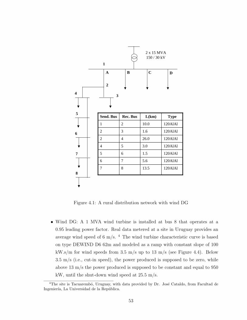
2 x 15 MVA150 / 30 kV

A B C D

1

2

34

5

6

7

8120AlAl13.587

120AlAl5.676

120AlAl1.565

120AlAl3.054

120AlAl26.042

120AlAl1.632

120AlAl10.021

TypeL(km)Rec. BusSend. Bus

Figure 4.1: A rural distribution network with wind DG

• Wind DG: A 1 MVA wind turbine is installed at bus 8 that operates at a

0.95 leading power factor. Real data metered at a site in Uruguay provides an

average wind speed of 6 m/s. 4 The wind turbine characteristic curve is based

on type DEWIND D6 62m and modeled as a ramp with constant slope of 100

kW.s/m for wind speeds from 3.5 m/s up to 13 m/s (see Figure 4.4). Below

3.5 m/s (i.e., cut-in speed), the power produced is supposed to be zero, while

above 13 m/s the power produced is supposed to be constant and equal to 950

kW, until the shut-down wind speed at 25.5 m/s.

4The site is Tacuarembo, Uruguay, with data provided by Dr. Jose Cataldo, from Facultad deIngenierıa, La Universidad de la Republica.

53

0

500

1000

1500

2000

2500

3000

3500

4000

4500

0 4 8 12 16 20 24

Ind_Sum_Working

Ind_Aut_Working

Ind_Win_Working

Ind_Sp_Working

0

20

40

60

80

100

120

140

160

180

0 4 8 12 16 20 24

Ind_Sum_Weekends

Ind_Aut_WeekendsInd_Win_Weekends

Ind_Sp_Weekends

P(kW)

P(kW)

Hr

Hr

Figure 4.2: Daily load profiles for the industrial customer

• Wind DG of different capacity factors with the same type of wind turbine as

before but changing the average wind speeds to obtain the different capacity

factors.

For the cases of intermittent DG, wind has been assumed to have a Rayleigh

distribution with the average equal to the real average wind speed measured as cited

above (Mendez et al., 2002). The simulations were performed using the Monte Carlo

technique running 10,000 draws from the distribution for each hour of each day for

each of the four seasons.

54

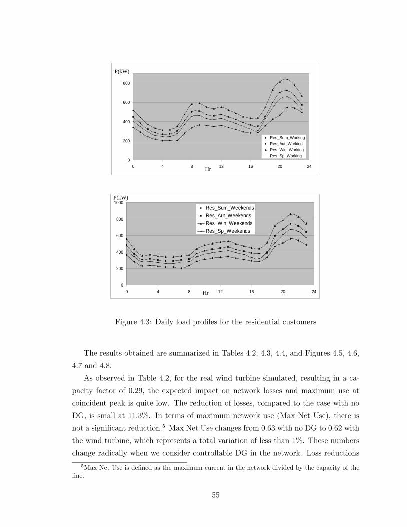
0

200

400

600

800

0 4 8 12 16 20 24

Res_Sum_Working

Res_Aut_WorkingRes_Win_Working

Res_Sp_Working

0

200

400

600

800

1000

0 4 8 12 16 20 24

Res_Sum_WeekendsRes_Aut_WeekendsRes_Win_WeekendsRes_Sp_Weekends

P(kW)

P(kW)

Hr

Hr

Figure 4.3: Daily load profiles for the residential customers

The results obtained are summarized in Tables 4.2, 4.3, 4.4, and Figures 4.5, 4.6,

4.7 and 4.8.

As observed in Table 4.2, for the real wind turbine simulated, resulting in a ca-

pacity factor of 0.29, the expected impact on network losses and maximum use at

coincident peak is quite low. The reduction of losses, compared to the case with no

DG, is small at 11.3%. In terms of maximum network use (Max Net Use), there is

not a significant reduction.5 Max Net Use changes from 0.63 with no DG to 0.62 with

the wind turbine, which represents a total variation of less than 1%. These numbers

change radically when we consider controllable DG in the network. Loss reductions

5Max Net Use is defined as the maximum current in the network divided by the capacity of theline.

55

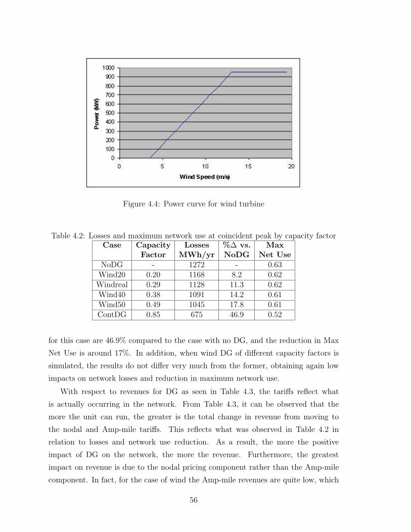
Figure 4.4: Power curve for wind turbine

Table 4.2: Losses and maximum network use at coincident peak by capacity factorCase Capacity Losses %∆ vs. Max

Factor MWh/yr NoDG Net UseNoDG - 1272 - 0.63Wind20 0.20 1168 8.2 0.62Windreal 0.29 1128 11.3 0.62Wind40 0.38 1091 14.2 0.61Wind50 0.49 1045 17.8 0.61ContDG 0.85 675 46.9 0.52

for this case are 46.9% compared to the case with no DG, and the reduction in Max

Net Use is around 17%. In addition, when wind DG of different capacity factors is

simulated, the results do not differ very much from the former, obtaining again low

impacts on network losses and reduction in maximum network use.

With respect to revenues for DG as seen in Table 4.3, the tariffs reflect what

is actually occurring in the network. From Table 4.3, it can be observed that the

more the unit can run, the greater is the total change in revenue from moving to

the nodal and Amp-mile tariffs. This reflects what was observed in Table 4.2 in

relation to losses and network use reduction. As a result, the more the positive

impact of DG on the network, the more the revenue. Furthermore, the greatest

impact on revenue is due to the nodal pricing component rather than the Amp-mile

component. In fact, for the case of wind the Amp-mile revenues are quite low, which

56

Table 4.3: DG Revenues in dollars per year and additional revenue from nodal pricingand Amp-mile

Case Cap. PSP Nodal Amp- (3)+(2) %∆Fac. only (2) mile -(1) vs. PSP

(1) (3)NoDG - 0 0 0 0 -Wind20 0.20 99729 105318 62 5651 5.7Windreal 0.29 144554 151780 110 7336 5.1Wind40 0.38 188376 197067 163 8854 4.7Wind50 0.49 246138 256153 247 10262 4.2ContDG 0.85 428590 456400 2696 30506 7.1

Table 4.4: Total charges to load in dollars per yearCase Cap. Charges MS Remaining Total

Factor Nodal (1) Network (2) (1)+(2)NoDG - 1778890 101740 32897 1811787Wind20 0.20 1769224 93366 41336 1810560Windreal 0.29 1764979 90110 44641 1809620Wind40 0.38 1760939 87151 47651 1808590Wind50 0.49 1755579 83426 51461 1807040ContDG 0.85 1719300 53478 83858 1803158

will be further discussed later. In percentage terms, because of the intermittent

nature of wind and the likelihood it will not be running when it is most valuable to

the system, its additional revenues are quite small in total and amount to 4-6% of

the revenue gained from only receiving prices at the PSP. In contrast, in percentage

terms, the controllable DG does better than wind even starting from a larger base.

The reason for this is the wind turbine is a consumer of reactive power, operating at

0.95 leading power factor, and must pay for reactive power.6 The controllable DG

resource operates at a 0.95 lagging power factor and is supplying reactive power to

the system for which it is paid. Moreover, the low impact on network use due to

the random characteristic of wind generation is expressed in monetary terms as a

low revenue through network charges to DG. Even for capacity factors of 0.5 the DG

revenue for contributing to reduce network use (e.g. $247/yr.) is less than 10% of

the revenue obtained by controllable DG (e.g. $2696/yr.) reflecting the fact that it

is not expected to be running at peak times to reduce line utilization.

6With power electronic devices applied to wind turbines this could not be the case. It is possibleto have both leading or lagging power factors.

57

Regarding charges to loads on the network as shown in Table 4.4, total charges

collected from loads decrease as the DG capacity factor increases, but even with

controllable DG the percentage reduction in total charges to loads is less than 0.5%.

This decrease, be it ever so slight, is taking place as the total fixed network costs are

increasing due to payments to DG for freeing up network capacity! It is also worth

noting that as DG runs at higher capacity factors, the nodal price charges decrease,

but this implies a lower merchandising surplus (MS) that can be used to offset fixed

network charges as seen in Table 4.4, and thus leads to more of the fixed network cost

being allocated through the Amp-mile method.

The pattern of nodal active power prices is shown in Figures 4.5 and 4.6. The

price curve for the case of intermittent DG is in between the curves for no DG and

controllable DG as would be expected because intermittent DG will provide some

reduction in nodal prices, but not to the same extent as with controllable DG. For

instance, in winter at weekdays, at node 8 (Figure 4.5), without DG, peak active

power prices are just above $92/MWh, while with controllable DG, peak active power

prices decrease to around $87/MWh. For the same case, with intermittent DG, at

0.29 capacity factor, expected peak prices are around $91/MWh. Once again, the

effect of intermittent DG is relatively low in expectation. Similar price behavior can

be observed at node 4. In Figure 4.6 is it can be observed that prices are higher

without DG and lower with controllable DG, being the prices with intermittent DG

in between them. However, it is important to note without DG, prices are higher at

node 8 than node 4 as node 8 is further away from the PSP. This reflects the higher

impact of distant nodes on network losses. A similar price behavior can be seen with

intermittent DG. However, if node 4 and node 8 are compared when controllable

DG is running at node 8 for the same season and time, then a different pattern is

observed. Because DG is reversing the power flows in circuits 6-7 and 7-8, the price

at node 4 is higher than the price at node 8.

A different pattern emerges with respect to nodal reactive power prices as seen

in Figures 4.7 and 4.8. Because wind DG operates at a leading power factor, nodal

reactive power prices are even higher with intermittent wind DG than without any

DG at all. For instance, in Figure for winter weekdays, at node 8 without DG,

peak reactive power prices are around $9.50/MVArh, while with controllable DG,

peak reactive power prices are nearly $7/MVArh. For this case, with intermittent

DG, peak reactive power prices are slightly higher than the $9.50/MVArh obtained

58

without DG. Consequently, as discussed above, the additional revenues available to

DG are eroded somewhat by the need for wind to purchase reactive power from the

system. In Figure 4.8 similar price patterns can be observed. Peak reactive power

prices are higher without DG than with controllable DG, but with intermittent DG

they are slightly higher than without DG. When comparing nodes 8 and 4, reactive

power prices do not vary as much as active power prices do between nodes.

Finally, it is worth observing the shape of the prices curves (Figures 4.5, 4.6, 4.7

and 4.8) and the load profile curves (Figures 4.2 and 4.3) are quite similar. Nodal

prices follows the load, which means that at times of higher load, nodal prices are

higher, while at times of lower load, nodal prices are lower. The signal sent by nodal

prices is clear both for loads and generators. When the network is more loaded, prices

are high, which gives the incentive to demand customers to consume less power. For

the case of generators, these high prices give them the incentive to produce more

power.

4.4 Amp-mile: Time Differentiated Charges vs.

Fixed Yearly Charges at Coincident Peak

In this section the difference between time differentiated charges and fixed charges

are examined within the Amp-mile method. A benchmark for comparison is the per

MWh charge where the fixed cost of the network is averaged over all load for the entire

year without regard to location or peak load. This yields a charge of $5.40/MWh and

the yearly charges for each bus can be seen in Table 4.5. Because nodes 3, 5, 6, 7,

and 8 have the same load profiles, their yearly charges are identical in the benchmark

case. For all cases there is no load at busses 1 and 2, and there is no need to report

any results for those busses.

To make matters simple for the ease of comparison, the merchandising surplus is

not used to offset the fixed cost. That is, the network fixed cost to be allocated has

been taken in full (i.e. $134.640). In addition, the simulations were conducted either

considering no DG in the network or fully controllable DG with the characteristics

used in section 4.3.

As expected, residential customers’ (i.e. same load profiles) locational charges

increase with the distance between the customer and the PSP. The more circuits over

which power demanded at bus k must travel, the greater is the charge. This reflects

59

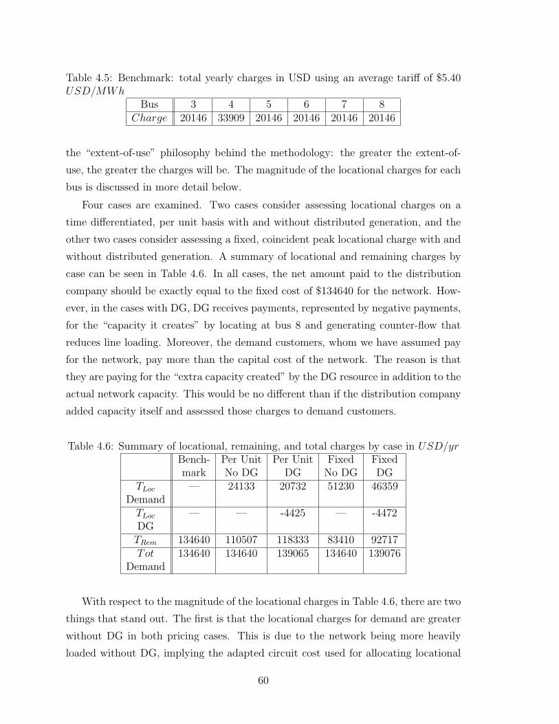
Table 4.5: Benchmark: total yearly charges in USD using an average tariff of $5.40USD/MWh

Bus 3 4 5 6 7 8Charge 20146 33909 20146 20146 20146 20146

the “extent-of-use” philosophy behind the methodology: the greater the extent-of-

use, the greater the charges will be. The magnitude of the locational charges for each

bus is discussed in more detail below.

Four cases are examined. Two cases consider assessing locational charges on a

time differentiated, per unit basis with and without distributed generation, and the

other two cases consider assessing a fixed, coincident peak locational charge with and

without distributed generation. A summary of locational and remaining charges by

case can be seen in Table 4.6. In all cases, the net amount paid to the distribution

company should be exactly equal to the fixed cost of $134640 for the network. How-

ever, in the cases with DG, DG receives payments, represented by negative payments,

for the “capacity it creates” by locating at bus 8 and generating counter-flow that

reduces line loading. Moreover, the demand customers, whom we have assumed pay

for the network, pay more than the capital cost of the network. The reason is that

they are paying for the “extra capacity created” by the DG resource in addition to the

actual network capacity. This would be no different than if the distribution company

added capacity itself and assessed those charges to demand customers.

Table 4.6: Summary of locational, remaining, and total charges by case in USD/yrBench- Per Unit Per Unit Fixed Fixedmark No DG DG No DG DG

TLoc — 24133 20732 51230 46359Demand

TLoc — — -4425 — -4472DGTRem 134640 110507 118333 83410 92717Tot 134640 134640 139065 134640 139076

Demand

With respect to the magnitude of the locational charges in Table 4.6, there are two

things that stand out. The first is that the locational charges for demand are greater

without DG in both pricing cases. This is due to the network being more heavily

loaded without DG, implying the adapted circuit cost used for allocating locational

60

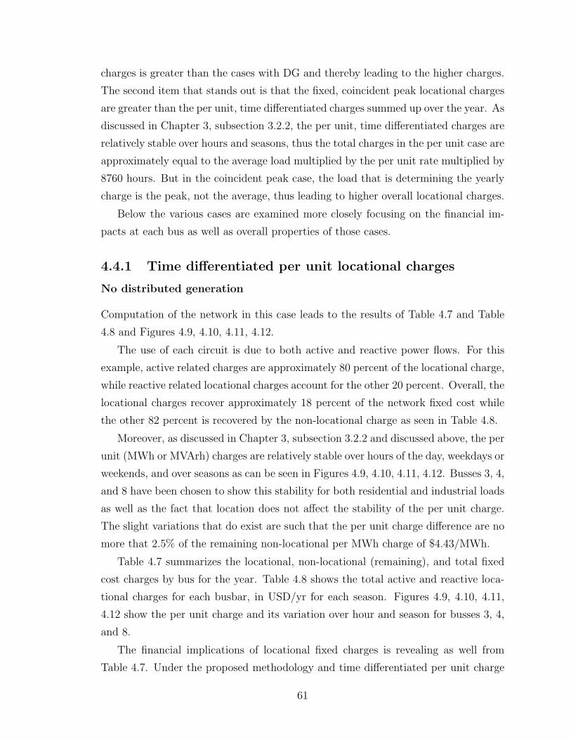
charges is greater than the cases with DG and thereby leading to the higher charges.

The second item that stands out is that the fixed, coincident peak locational charges

are greater than the per unit, time differentiated charges summed up over the year. As

discussed in Chapter 3, subsection 3.2.2, the per unit, time differentiated charges are

relatively stable over hours and seasons, thus the total charges in the per unit case are

approximately equal to the average load multiplied by the per unit rate multiplied by

8760 hours. But in the coincident peak case, the load that is determining the yearly

charge is the peak, not the average, thus leading to higher overall locational charges.

Below the various cases are examined more closely focusing on the financial im-

pacts at each bus as well as overall properties of those cases.

4.4.1 Time differentiated per unit locational charges

No distributed generation

Computation of the network in this case leads to the results of Table 4.7 and Table

4.8 and Figures 4.9, 4.10, 4.11, 4.12.

The use of each circuit is due to both active and reactive power flows. For this

example, active related charges are approximately 80 percent of the locational charge,

while reactive related locational charges account for the other 20 percent. Overall, the

locational charges recover approximately 18 percent of the network fixed cost while

the other 82 percent is recovered by the non-locational charge as seen in Table 4.8.

Moreover, as discussed in Chapter 3, subsection 3.2.2 and discussed above, the per

unit (MWh or MVArh) charges are relatively stable over hours of the day, weekdays or

weekends, and over seasons as can be seen in Figures 4.9, 4.10, 4.11, 4.12. Busses 3, 4,

and 8 have been chosen to show this stability for both residential and industrial loads

as well as the fact that location does not affect the stability of the per unit charge.

The slight variations that do exist are such that the per unit charge difference are no

more that 2.5% of the remaining non-locational per MWh charge of $4.43/MWh.

Table 4.7 summarizes the locational, non-locational (remaining), and total fixed

cost charges by bus for the year. Table 4.8 shows the total active and reactive loca-

tional charges for each busbar, in USD/yr for each season. Figures 4.9, 4.10, 4.11,

4.12 show the per unit charge and its variation over hour and season for busses 3, 4,

and 8.

The financial implications of locational fixed charges is revealing as well from

Table 4.7. Under the proposed methodology and time differentiated per unit charge

61

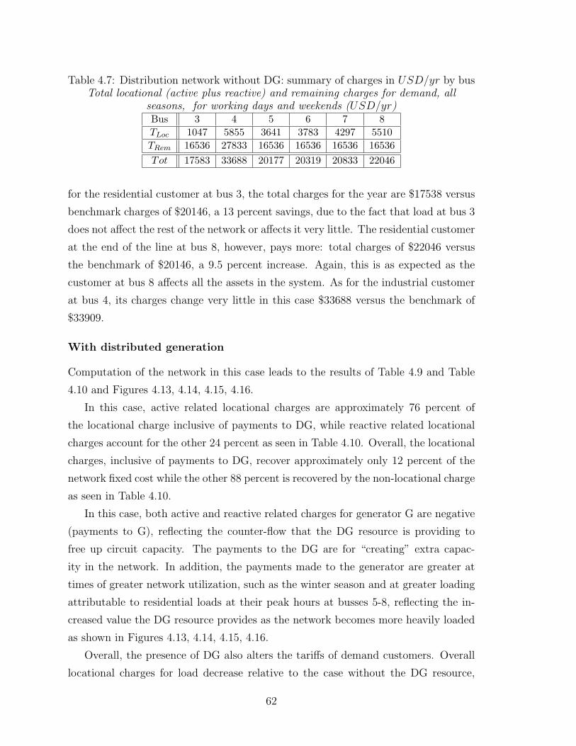
Table 4.7: Distribution network without DG: summary of charges in USD/yr by busTotal locational (active plus reactive) and remaining charges for demand, all

seasons, for working days and weekends (USD/yr)Bus 3 4 5 6 7 8TLoc 1047 5855 3641 3783 4297 5510TRem 16536 27833 16536 16536 16536 16536Tot 17583 33688 20177 20319 20833 22046

for the residential customer at bus 3, the total charges for the year are $17538 versus

benchmark charges of $20146, a 13 percent savings, due to the fact that load at bus 3

does not affect the rest of the network or affects it very little. The residential customer

at the end of the line at bus 8, however, pays more: total charges of $22046 versus

the benchmark of $20146, a 9.5 percent increase. Again, this is as expected as the

customer at bus 8 affects all the assets in the system. As for the industrial customer

at bus 4, its charges change very little in this case $33688 versus the benchmark of

$33909.

With distributed generation

Computation of the network in this case leads to the results of Table 4.9 and Table

4.10 and Figures 4.13, 4.14, 4.15, 4.16.

In this case, active related locational charges are approximately 76 percent of

the locational charge inclusive of payments to DG, while reactive related locational

charges account for the other 24 percent as seen in Table 4.10. Overall, the locational

charges, inclusive of payments to DG, recover approximately only 12 percent of the

network fixed cost while the other 88 percent is recovered by the non-locational charge

as seen in Table 4.10.

In this case, both active and reactive related charges for generator G are negative

(payments to G), reflecting the counter-flow that the DG resource is providing to

free up circuit capacity. The payments to the DG are for “creating” extra capac-

ity in the network. In addition, the payments made to the generator are greater at

times of greater network utilization, such as the winter season and at greater loading

attributable to residential loads at their peak hours at busses 5-8, reflecting the in-

creased value the DG resource provides as the network becomes more heavily loaded

as shown in Figures 4.13, 4.14, 4.15, 4.16.

Overall, the presence of DG also alters the tariffs of demand customers. Overall

locational charges for load decrease relative to the case without the DG resource,

62

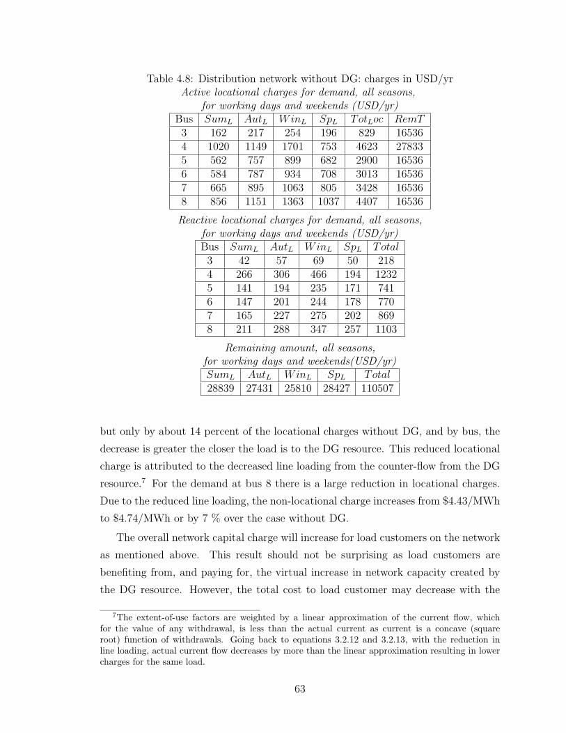
Table 4.8: Distribution network without DG: charges in USD/yrActive locational charges for demand, all seasons,

for working days and weekends (USD/yr)Bus SumL AutL WinL SpL TotLoc RemT3 162 217 254 196 829 165364 1020 1149 1701 753 4623 278335 562 757 899 682 2900 165366 584 787 934 708 3013 165367 665 895 1063 805 3428 165368 856 1151 1363 1037 4407 16536

Reactive locational charges for demand, all seasons,for working days and weekends (USD/yr)Bus SumL AutL WinL SpL Total3 42 57 69 50 2184 266 306 466 194 12325 141 194 235 171 7416 147 201 244 178 7707 165 227 275 202 8698 211 288 347 257 1103

Remaining amount, all seasons,for working days and weekends(USD/yr)SumL AutL WinL SpL Total28839 27431 25810 28427 110507

but only by about 14 percent of the locational charges without DG, and by bus, the

decrease is greater the closer the load is to the DG resource. This reduced locational

charge is attributed to the decreased line loading from the counter-flow from the DG

resource.7 For the demand at bus 8 there is a large reduction in locational charges.

Due to the reduced line loading, the non-locational charge increases from $4.43/MWh

to $4.74/MWh or by 7 % over the case without DG.

The overall network capital charge will increase for load customers on the network

as mentioned above. This result should not be surprising as load customers are

benefiting from, and paying for, the virtual increase in network capacity created by

the DG resource. However, the total cost to load customer may decrease with the

7The extent-of-use factors are weighted by a linear approximation of the current flow, whichfor the value of any withdrawal, is less than the actual current as current is a concave (squareroot) function of withdrawals. Going back to equations 3.2.12 and 3.2.13, with the reduction inline loading, actual current flow decreases by more than the linear approximation resulting in lowercharges for the same load.

63

Table 4.9: Distribution network with DG: summary of charges in USD/yr by busTotal locational (active plus reactive) and remaining charges for demand, all

seasons, for working days and weekends (USD/yr)Bus 3 4 5 6 7 8D 8GTLoc 1033 5704 3535 3648 3809 3003 -4425TRem 17706 29801 17706 17706 17706 17706 -

Tot 18739 35505 21241 21354 21515 20709 -4425

decrease in line losses induced by the increased network capacity as shown in Table

4.4, though losses are not examined in this section. The total charges paid by load

for network fixed costs, relative to the benchmark are all higher, except for bus 3, and

they are all higher than the case without DG except for bus 8 which benefits directly

from being at the same bus as DG.

4.4.2 Fixed, coincident peak locational charges

No distributed generation

A summary of the fixed, coincident peak locational charges without DG can be found

in Table 4.11 and Table 4.13. As discussed above, the total charges paid, relative to

the time differentiated per unit charges, will depend on whether the load for a partic-

ular bus at the coincident peak is less than or greater than the average load over the

year. For example, the loads at all residential (3,5,6,7,8) busses pay lower locational

charges, and lower overall charges, than they did under the time differentiated pricing

regime because their load at the coincident peak hour is less than the average load

over the year. The overall charges for residential loads are also much lower than the

benchmark charges. In fact, the coincident peak occurs in hour 3 during the winter

season, and is driven by the industrial customer at bus 4. Moreover, from the load

profiles in Figures 4.2 and 4.3, it is easy to see that at the peak hour, residential

customers are close to their minimums rather than their peaks. This result is purely

an artifact of the load data from Uruguay. If the residential customers peaked at

about the same time as the industrial customer, they too would pay more than under

the per unit charges just as the industrial customer at bus 4 does. The industrial

customer, because it is driving the peak, pays more than six times more in locational

charges than it did under the other pricing mechanism, and drives the overall more

than doubling in locational charges.

64

Table 4.10: Distribution network with DG: charges in USD/yrActive locational charges for demand and generation,all seasons, for working days and weekends(USD/yr)Bus SumL AutL WinL SpL TotLoc RemT3 156 211 249 190 806 177064 973 1105 1641 717 4436 298015 511 716 860 637 2724 177066 519 738 889 653 2799 177067 492 754 946 649 2841 17706

8-dem 310 532 728 438 2008 177068-gen -626 -844 -999 -754 -3223 -

Reactive locational charges for demand and generation,for working days and weekends (USD/yr)Bus SumL AutL WinL SpL Total3 45 59 70 53 2274 282 314 465 207 12685 165 210 244 192 8116 172 220 256 201 8497 188 254 298 228 968

8-dem 181 260 328 226 9958-gen -279 -304 -327 -292 -1202

Remaining amount, all seasons,for working days and weekends(USD/yr)SumL AutL WinL SpL Total30571 29435 28012 30315 118333

With distributed generation

Much like the time differentiated, per unit pricing scheme with distributed generation,

distributed generation leads to an overall decrease of 10 percent in locational charges

for loads, and that decrease is greater for busses closer to the DG resource. Moreover,

the overall network capital charge will increase, as it did in the previous pricing

scheme, for load customers on the network. Again, load customers are benefiting

from, and paying for, the virtual increase in network capacity created by the DG

resource. It is interesting to note that the DG resources revenues from creating extra

capacity have changed little, increasing by just over 1 percent. For loads, the overall

charges have increased versus fixed charges without DG, except for loads at busses 7

and 8 which benefit greatly from the presence of DG at peak. Just as before under

fixed charges without DG, the residential busses pay far less than the benchmark,

65

Table 4.11: Distribution network without DG: summary of peak charges in USD/yrTotal locational (active plus reactive) and remaining charges for demand, all

seasons, for working days and weekends (USD/yr)Bus 3 4 5 6 7 8 TOT

TotLoc 827 36230 3039 3145 3535 4455 51230TotRem 4675 60035 4675 4675 4675 4675 83410

Tot 5502 96265 7714 7820 8210 9130 134640

Table 4.12: Distribution network with DG: summary of peak charges in USD/yrTotal locational and remaining charges for demand, all seasons, for working days

and weekends (USD/yr)Bus 3 4 5 6 7 8D 8G

TotLoc 819 35200 2940 3004 2668 1764 -4472TotRem 5196 66737 5196 5196 5196 5196 -

Tot 6015 101937 8136 8200 7864 6960 -4472

and far less than under the per unit prices.

4.5 Chapter Concluding Remarks

For the case study, it has been shown the DG resource can provide benefits to the

network through reduced line losses and line loading by 47 perecent and 17 percent

respectively. DG resources are rewarded, through nodal pricing as can be seen by the

revenue in Table 4.3, for providing such benefits to the distribution system. From

Figures 4.5, 4.6, 4.7, 4.8 the price impact of losses with and without the DG resource,

and with DG resources of different capacity factors can be observed.

Without the incentives provided by nodal pricing through higher prices leading to

larger revenues for DG resources, there is less opportunity of inducing DG resources

to locate and operate so they can provide the system benefits as shown above. Given

worldwide experience with nodal pricing, and the fact that DG resources transform

the distribution network into an active network like transmission, it makes sense to

consider nodal pricing in distribution.

In relation to the Amp-mile proposed methodology applied to the model network,

the financial incentives are in the desired direction, and the signals are strongest

for those loads that drive the coincident peak of the system, and that are far away

from the power supply point. Using a fixed, coincident peak charge recovers more of

the fixed costs through locational charges than does a time differentiated, per unit

66

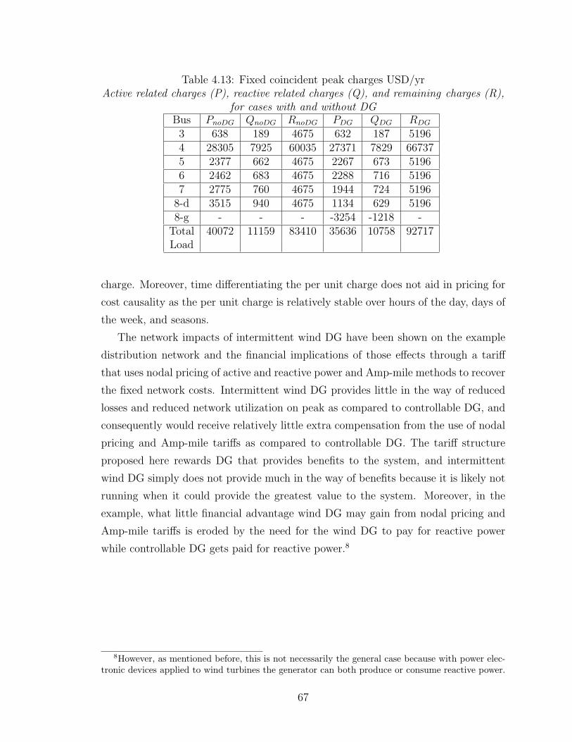
Table 4.13: Fixed coincident peak charges USD/yrActive related charges (P), reactive related charges (Q), and remaining charges (R),

for cases with and without DGBus PnoDG QnoDG RnoDG PDG QDG RDG

3 638 189 4675 632 187 51964 28305 7925 60035 27371 7829 667375 2377 662 4675 2267 673 51966 2462 683 4675 2288 716 51967 2775 760 4675 1944 724 5196

8-d 3515 940 4675 1134 629 51968-g - - - -3254 -1218 -

Total 40072 11159 83410 35636 10758 92717Load

charge. Moreover, time differentiating the per unit charge does not aid in pricing for

cost causality as the per unit charge is relatively stable over hours of the day, days of

the week, and seasons.

The network impacts of intermittent wind DG have been shown on the example

distribution network and the financial implications of those effects through a tariff

that uses nodal pricing of active and reactive power and Amp-mile methods to recover

the fixed network costs. Intermittent wind DG provides little in the way of reduced

losses and reduced network utilization on peak as compared to controllable DG, and

consequently would receive relatively little extra compensation from the use of nodal

pricing and Amp-mile tariffs as compared to controllable DG. The tariff structure

proposed here rewards DG that provides benefits to the system, and intermittent

wind DG simply does not provide much in the way of benefits because it is likely not

running when it could provide the greatest value to the system. Moreover, in the

example, what little financial advantage wind DG may gain from nodal pricing and

Amp-mile tariffs is eroded by the need for the wind DG to pay for reactive power

while controllable DG gets paid for reactive power.8

8However, as mentioned before, this is not necessarily the general case because with power elec-tronic devices applied to wind turbines the generator can both produce or consume reactive power.

67

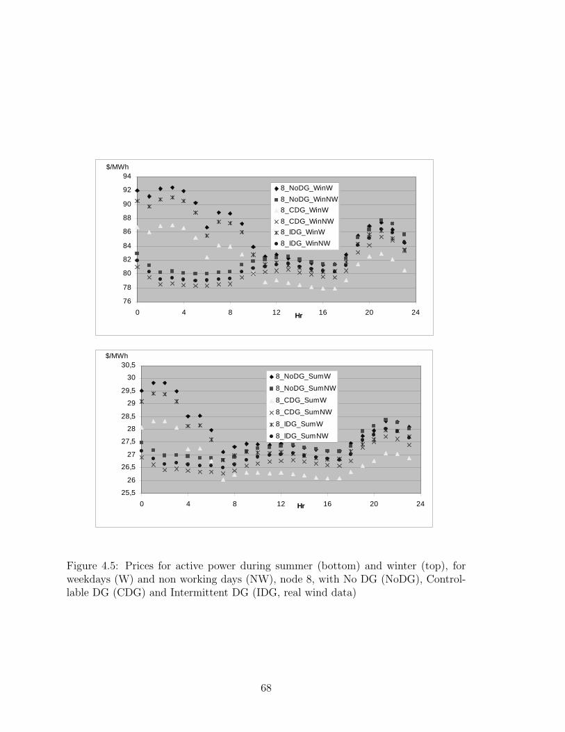
76

78

80

82

84

86

88

90

92

94

0 4 8 12 16 20 24Hr

8_NoDG_WinW

8_NoDG_WinNW

8_CDG_WinW

8_CDG_WinNW

8_IDG_WinW

8_IDG_WinNW

25,5

26

26,5

27

27,5

28

28,5

29

29,5

30

30,5

0 4 8 12 16 20 24Hr

8_NoDG_SumW

8_NoDG_SumNW

8_CDG_SumW

8_CDG_SumNW

8_IDG_SumW

8_IDG_SumNW

$/MWh

$/MWh

Figure 4.5: Prices for active power during summer (bottom) and winter (top), forweekdays (W) and non working days (NW), node 8, with No DG (NoDG), Control-lable DG (CDG) and Intermittent DG (IDG, real wind data)

68

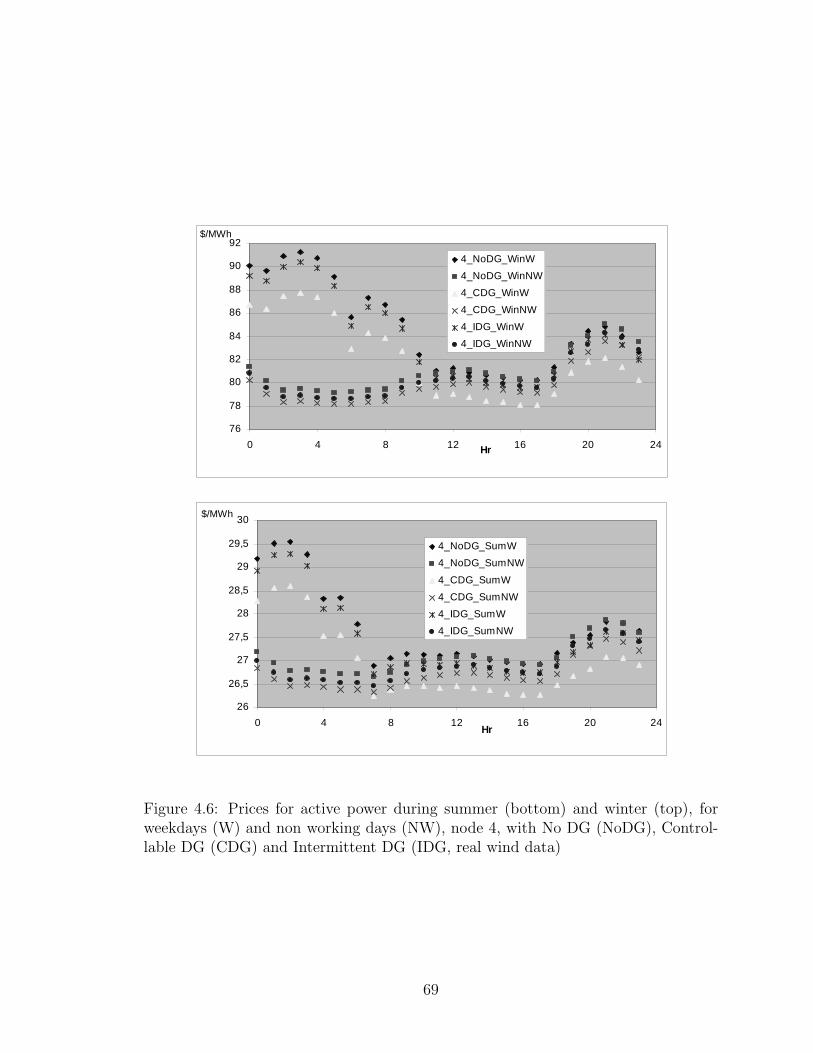
76

78

80

82

84

86

88

90

92

0 4 8 12 16 20 24Hr

4_NoDG_WinW

4_NoDG_WinNW

4_CDG_WinW

4_CDG_WinNW

4_IDG_WinW

4_IDG_WinNW

26

26,5

27

27,5

28

28,5

29

29,5

30

0 4 8 12 16 20 24Hr

4_NoDG_SumW

4_NoDG_SumNW

4_CDG_SumW

4_CDG_SumNW

4_IDG_SumW

4_IDG_SumNW

$/MWh

$/MWh

Figure 4.6: Prices for active power during summer (bottom) and winter (top), forweekdays (W) and non working days (NW), node 4, with No DG (NoDG), Control-lable DG (CDG) and Intermittent DG (IDG, real wind data)

69

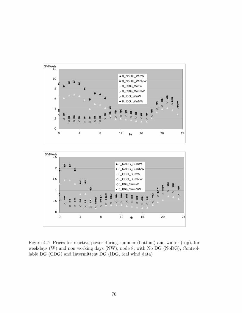
0

2

4

6

8

10

12

0 4 8 12 16 20 24Hr

8_NoDG_WinW

8_NoDG_WinNW

8_CDG_WinW

8_CDG_WinNW

8_IDG_WinW

8_IDG_WinNW

0

0,5

1

1,5

2

2,5

0 4 8 12 16 20 24Hr

8_NoDG_SumW

8_NoDG_SumNW

8_CDG_SumW

8_CDG_SumNW

8_IDG_SumW

8_IDG_SumNW

$/MVArh

$/MVArh

Figure 4.7: Prices for reactive power during summer (bottom) and winter (top), forweekdays (W) and non working days (NW), node 8, with No DG (NoDG), Control-lable DG (CDG) and Intermittent DG (IDG, real wind data)

70

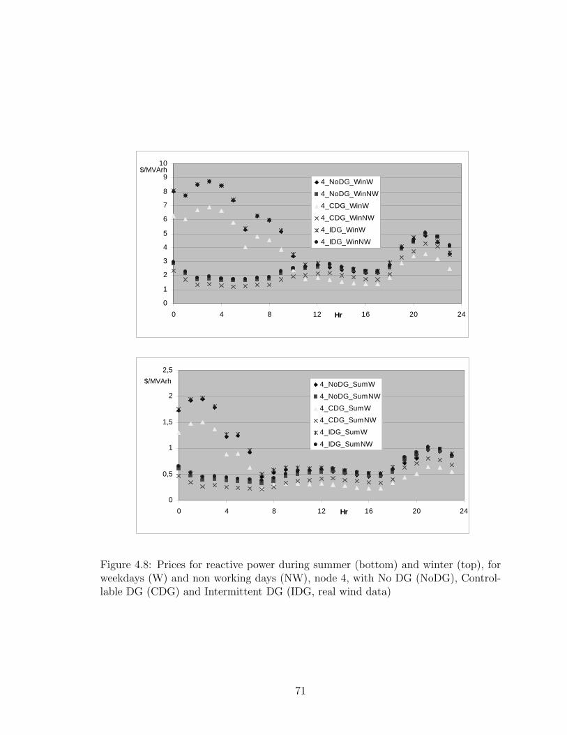
0

1

2

3

4

5

6

7

8

9

10

0 4 8 12 16 20 24Hr

4_NoDG_WinW

4_NoDG_WinNW

4_CDG_WinW

4_CDG_WinNW

4_IDG_WinW

4_IDG_WinNW

0

0,5

1

1,5

2

2,5

0 4 8 12 16 20 24Hr

4_NoDG_SumW

4_NoDG_SumNW

4_CDG_SumW

4_CDG_SumNW

4_IDG_SumW

4_IDG_SumNW

$/MVArh

$/MVArh

Figure 4.8: Prices for reactive power during summer (bottom) and winter (top), forweekdays (W) and non working days (NW), node 4, with No DG (NoDG), Control-lable DG (CDG) and Intermittent DG (IDG, real wind data)

71

0,00

0,20

0,40

0,60

0,80

1,00

1,20

0 4 8 12 16 20 24

Node3_SumW

Node3_SumNW

Node4_SumW

Node4_SumNW

Node8_SumW

Node8_SumNW

USD/MWh

Hr

RemT = 4.43 USD/MWh

0,00

0,20

0,40

0,60

0,80

1,00

1,20

0 4 8 12 16 20 24

Node3_WinW

Node3_WinNW

Node4_WinW

Node4_WinNW

Node8_WinW

Node8_WinNW

USD/MWh

Hr

RemT = 4.43 USD/MWh

Figure 4.9: Active locational tariffs for demand during summer (top) and winter (bot-tom), for working (W) and non-working days (NW), nodes 3, 4 and 8 (USD/MWh)

72

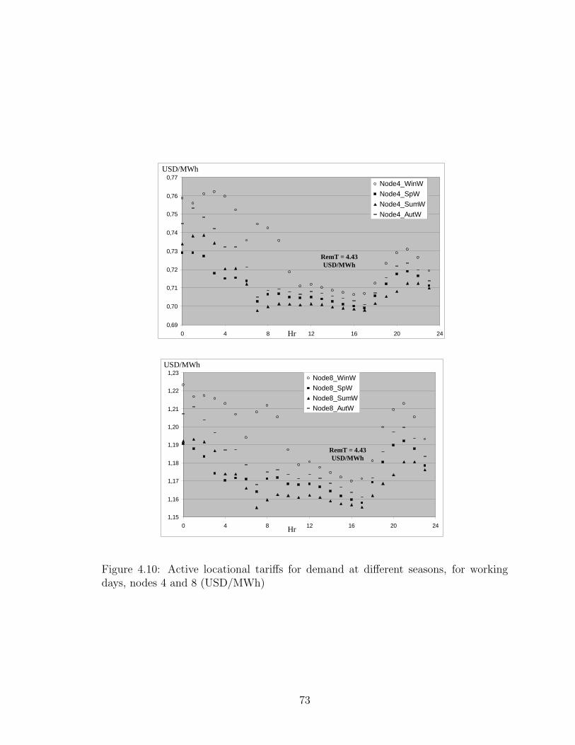
0,69

0,70

0,71

0,72

0,73

0,74

0,75

0,76

0,77

0 4 8 12 16 20 24

Node4_WinW

Node4_SpW

Node4_SumW

Node4_AutW

1,15

1,16

1,17

1,18

1,19

1,20

1,21

1,22

1,23

0 4 8 12 16 20 24

Node8_WinW

Node8_SpW

Node8_SumW

Node8_AutW

USD/MWh

USD/MWh

Hr

Hr

RemT = 4.43 USD/MWh

RemT = 4.43 USD/MWh

Figure 4.10: Active locational tariffs for demand at different seasons, for workingdays, nodes 4 and 8 (USD/MWh)

73

0,00

0,20

0,40

0,60

0,80

0 4 8 12 16 20 24

Node3_SumW

Node3_SumNW

Node4_SumW

Node4_SumNW

Node8_SumW

Node8_SumNW

0,00

0,20

0,40

0,60

0,80

0 4 8 12 16 20 24

Node3_WinW

Node3_WinNW

Node4_WinW

Node4_WinNW

Node8_WinW

Node8_WinNW

USD/MVArh

USD/MVArh

Hr

Hr

Figure 4.11: Reactive locational tariffs for demand during summer (top) and win-ter (bottom), for working (W) and non-working days (NW), nodes 3, 4 and 8(USD/MVArh)

74

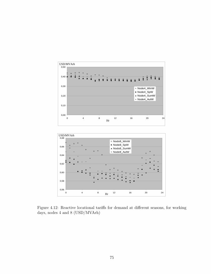
0,00

0,10

0,20

0,30

0,40

0,50

0 4 8 12 16 20 24

Node4_WinW

Node4_SpWNode4_SumW

Node4_AutW

0,56

0,58

0,60

0,62

0,64

0,66

0,68

0 4 8 12 16 20 24

Nodo8_WinWNode8_SpW

Nodo8_SumWNode8_AutW

USD/MVArh

USD/MVArh

Hr

Hr

Figure 4.12: Reactive locational tariffs for demand at different seasons, for workingdays, nodes 4 and 8 (USD/MVArh)

75

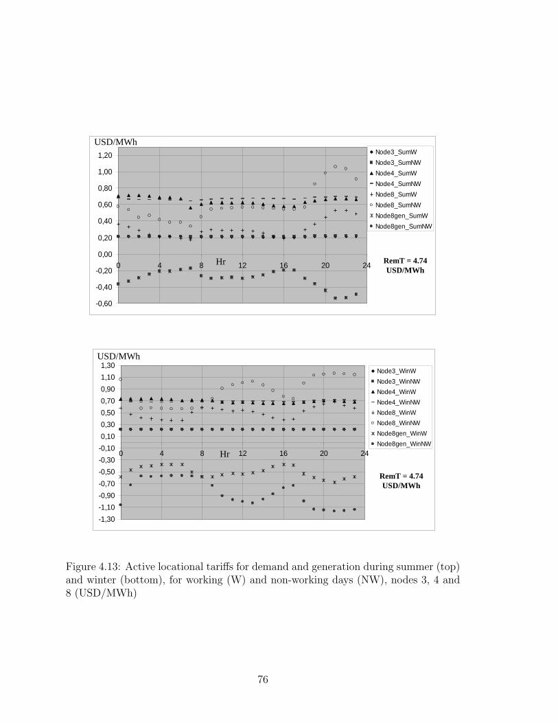
-0,60

-0,40

-0,20

0,00

0,20

0,40

0,60

0,80

1,00

1,20

0 4 8 12 16 20 24

Node3_SumW

Node3_SumNW

Node4_SumW

Node4_SumNW

Node8_SumW

Node8_SumNW

Node8gen_SumW

Node8gen_SumNW

-1,30

-1,10

-0,90

-0,70

-0,50

-0,30

-0,10

0,10

0,30

0,50

0,70

0,90

1,10

1,30

0 4 8 12 16 20 24

Node3_WinW

Node3_WinNW

Node4_WinW

Node4_WinNW

Node8_WinW

Node8_WinNW

Node8gen_WinW

Node8gen_WinNW

USD/MWh

USD/MWh

Hr

Hr

RemT = 4.74 USD/MWh

RemT = 4.74 USD/MWh

Figure 4.13: Active locational tariffs for demand and generation during summer (top)and winter (bottom), for working (W) and non-working days (NW), nodes 3, 4 and8 (USD/MWh)

76

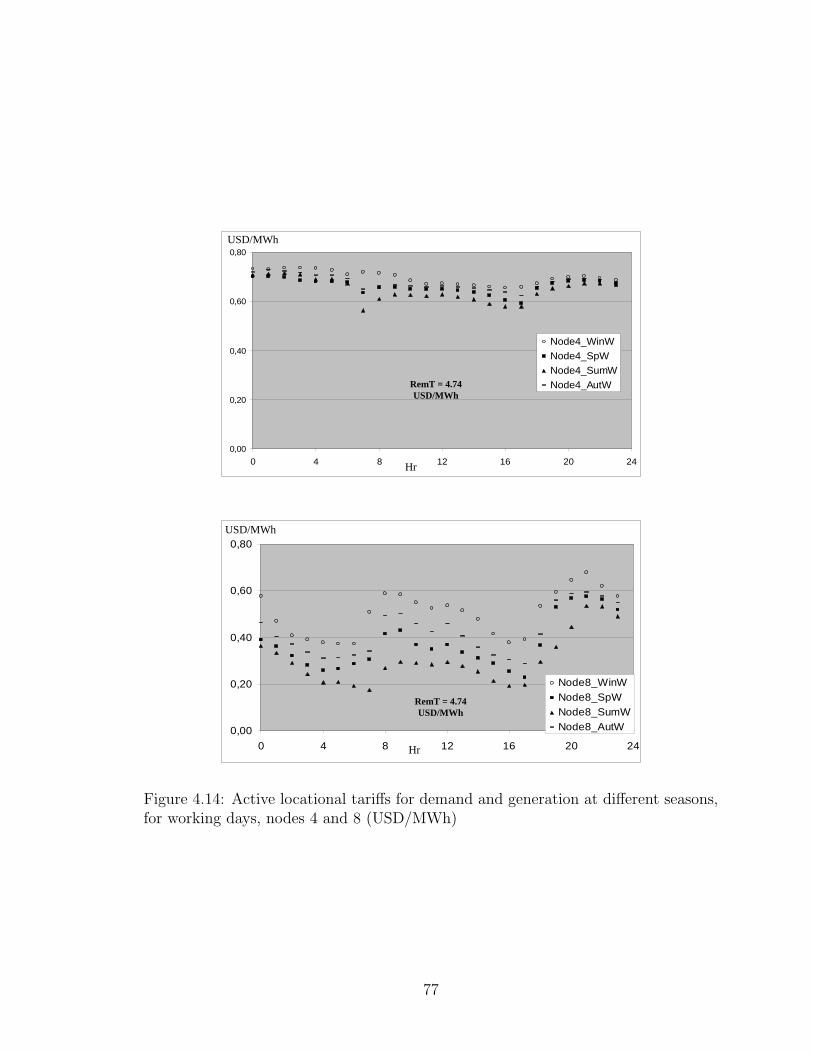
0,00

0,20

0,40

0,60

0,80

0 4 8 12 16 20 24

Node4_WinWNode4_SpWNode4_SumW

Node4_AutW

0,00

0,20

0,40

0,60

0,80

0 4 8 12 16 20 24

Node8_WinWNode8_SpWNode8_SumWNode8_AutW

USD/MWh

USD/MWh

Hr

Hr

RemT = 4.74 USD/MWh

RemT = 4.74 USD/MWh

Figure 4.14: Active locational tariffs for demand and generation at different seasons,for working days, nodes 4 and 8 (USD/MWh)

77

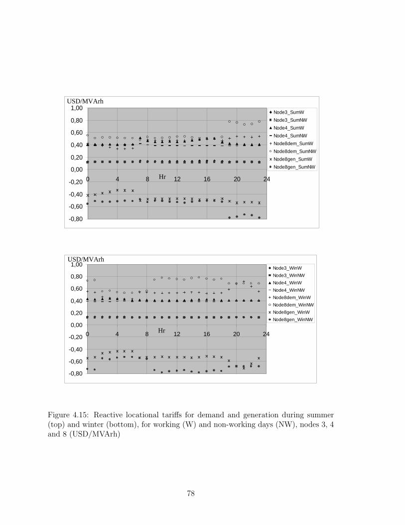
-0,80

-0,60

-0,40

-0,20

0,00

0,20

0,40

0,60

0,80

1,00

0 4 8 12 16 20 24

Node3_SumW

Node3_SumNW

Node4_SumW

Node4_SumNW

Node8dem_SumW

Node8dem_SumNW

Node8gen_SumW

Node8gen_SumNW

-0,80

-0,60

-0,40

-0,20

0,00

0,20

0,40

0,60

0,80

1,00

0 4 8 12 16 20 24

Node3_WinW

Node3_WinNW

Node4_WinW

Node4_WinNW

Node8dem_WinW

Node8dem_WinNW

Node8gen_WinW

Node8gen_WinNW

USD/MVArh

USD/MVArh

Hr

Hr

Figure 4.15: Reactive locational tariffs for demand and generation during summer(top) and winter (bottom), for working (W) and non-working days (NW), nodes 3, 4and 8 (USD/MVArh)

78

0,00

0,10

0,20

0,30

0,40

0,50

0,60

0 4 8 12 16 20 24

Node4_WinWNode4_SpW

Node4_SumWNode4_AutW

0,00

0,10

0,20

0,30

0,40

0,50

0,60

0,70

0,80

0 4 8 12 16 20 24

Nodo8_WinW

Node8_SpWNodo8_SumWNode8_AutW

USD/MVArh

USD/MVArh

Hr

Hr

Figure 4.16: Reactive locational tariffs for demand and generation at different seasons,for working days, nodes 4 and 8 (USD/MVArh)

79

80

Chapter 5

Towards a New Tariff Frameworkfor Distribution Networks 1

5.1 General Considerations

Moving from a traditional average cost tariff scheme for distribution networks in

which costs are allocated pro rata to cost reflective tariff scheme produces different

financial impacts on the network users. In this chapter the changes in distribution

charges in moving from a tariff that averages the cost of losses and fixed network

costs over all load to a cost-causality based tariff that uses nodal pricing to recover

the cost of losses and the proposed Amp-mile method to recover fixed network costs

through a locational charge based on the “extent of use” at the coincident peak is

examined. This study is quite important to determine which part of the tariff change

is the biggest driver for tariff differences. There are both locational and time-of-use

components in the proposed cost reflective tariff scheme that must be analyzed so it

can be determined what is exactly driving the changes in individual tariff charges. The

change can be decomposed into four components that are detailed in next section. The

decomposition analysis is undertaken accounting for the example system of Chapter

4, with DG, and without controllable DG located at bus 8.

5.2 Tariff Decomposition Results

Following the direct comparison of the average cost tariff to the proposed cost-

reflective tariff, I decompose the overall change in four steps to determine the following

effects separately.

1This chapter draws heavily in both text and concept from the published version of(Sotkiewicz, P.M. and Vignolo, J.M. 1/07, 2007).

81

1. Changes attributable to moving to peak network charges from averaging.

2. Changes attributable to moving to location-based peak network charges from

nonlocation-based peak network charges.

3. Changes attributable to moving to location and time-of-use based marginal

losses from averaging, and respecting the constraint that collections for losses

must equal the cost of losses.

4. Changes attributable to full marginal losses that potentially over-collect for

losses, but respecting the constraint that collections for costs must equal the

costs to be covered. This means any over-collections for losses reduce network

charges.

Additionally, the difference made by DG at each decomposition step is also shown.

5.2.1 Averaging losses and network costs

As seen in section 2.2.3, the average cost tariff charge for load at bus k for the year

is the sum of (2.2.1) and (2.2.3).

ACdk =

∑Tt=1 Pdtk∑T

t=1

∑nk=1 Pdtk

(∑

t

Losstλt +L∑

l=1

CCl). (5.2.1)

As DG resources are not charged for losses or network costs, it does not face

charges but collects revenue as defined by equation (2.2.2), which is the summation,

for all time periods, of the price of power at the PSP multiplied by the active power

output of the DG resource.

5.2.2 Averaging losses and coincident peak network costs

As seen in section 2.2.3, this tariff scheme is different from the averaging scheme only

in the charges for fixed network costs, which are based on coincident peak. The tariff

charge for the year under this scheme is the sum of (2.2.1) and (2.2.4).

ALCPdk =

∑Tt=1 Pdtk∑T

t=1

∑nk=1 Pdtk

∑t

Losstλt

+P peak

dk∑nk=1 P peak

dk

L∑

l=1

CCl. (5.2.2)

82

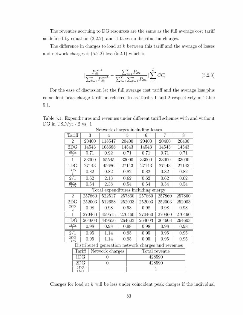
The revenues accruing to DG resources are the same as the full average cost tariff

as defined by equation (2.2.2), and it faces no distribution charges.

The difference in charges to load at k between this tariff and the average of losses

and network charges is (5.2.2) less (5.2.1) which is

[P peak

dk∑nk=1 P peak

dk

−∑T

t=1 Pdtk∑Tt=1

∑nk=1 Pdtk

]L∑

l=1

CCl (5.2.3)

For the ease of discussion let the full average cost tariff and the average loss plus

coincident peak charge tariff be referred to as Tariffs 1 and 2 respectively in Table

5.1.

Table 5.1: Expenditures and revenues under different tariff schemes with and withoutDG in USD/yr - 2 vs. 1

Network charges including lossesTariff 3 4 5 6 7 8

2 20400 118547 20400 20400 20400 204002DG 14543 108688 14543 14543 14543 145432DG

20.71 0.92 0.71 0.71 0.71 0.71

1 33000 55545 33000 33000 33000 330001DG 27143 45686 27143 27143 27143 271431DG

10.82 0.82 0.82 0.82 0.82 0.82

2/1 0.62 2.13 0.62 0.62 0.62 0.622DG1DG

0.54 2.38 0.54 0.54 0.54 0.54Total expenditures including energy

2 257860 522517 257860 257860 257860 2578602DG 252003 512658 252003 252003 252003 2520032DG

20.98 0.98 0.98 0.98 0.98 0.98

1 270460 459515 270460 270460 270460 2704601DG 264603 449656 264603 264603 264603 2646031DG

10.98 0.98 0.98 0.98 0.98 0.98

2/1 0.95 1.14 0.95 0.95 0.95 0.952DG1DG

0.95 1.14 0.95 0.95 0.95 0.95

Distributed generation network charges and revenuesTariff Network charges Total revenue1DG 0 4285902DG 0 4285902DG1DG

– 1

Charges for load at k will be less under coincident peak charges if the individual

83

share of load at coincident peak is less than the share of average load over the year,

or

P peakdk∑n

k=1 P peakdk

<

∑Tt=1 Pdtk∑T

t=1

∑nk=1 Pdtk

. (5.2.4)

Another way of expressing this is to say the load factor, defined by coincident peak,

is higher relative to other loads on the network, rewarding load that is relatively more

constant or has peaks counter-cyclic to the system peak. Conversely, charges will be

higher for those customers with relatively low load factors or have peaks coincident

with the system peak. Rearranging (5.2.4) yields

∑Tt=1

∑nk=1 Pdtk∑n

k=1 P peakdk

<

∑Tt=1 Pdtk

P peakdk

. (5.2.5)

Dividing both sides of (5.2.5) by 8760 hours yield the load factor result.

This result can be readily seen in Table 5.1 and looking back to Figures 4.2 and

4.3. Residential customers have relatively low loads at peak and in fact have peaks

that are countercyclical to the system peak. Consequently, their distribution tariff

charges are 38 percent and 46 percent lower without and with DG respectively than

under full averaging. However, the industrial customer who is driving the peak sees

its distribution tariff charges go up 113 percent and 138 percent without and with

DG respectively just by moving to allocation of fixed network costs based on the

peak. However, DG leads to lower overall distribution charges for both residential

and industrial customers relative to not having DG due to the reduction in line losses.

While the percent changes are large for distribution charges, as a percentage of total

charges, inclusive of energy, the changes are relatively much smaller with residential

customers seeing a 5 percent decline in overall charges while the industrial customer

sees a 14 percent increase both with and without DG. Still, moving to coincident

peak charges to recover network fixed costs has a large effect on who pays for those

costs versus averaging.

5.2.3 Averaging losses and Amp-mile network charges

This tariff scheme introduces locational aspects into recovery of the fixed cost portion

of network charges. The charge for load at bus k is the sum of (2.2.1), (3.2.26),

(3.2.28), and (3.2.32).

84

ALAMdk =

∑Tt=1 Pdtk∑T

t=1

∑nk=1 Pdtk

∑t

Losstλt

+L∑

l=1

(AEoUpeakdlk + REoUpeak

dlk )× ACCpeakl

+P peak

dk∑nk=1 P peak

dk

RCCpeak. (5.2.6)

DG pays a charge for its extent of use

L∑

l=1

(AEoUpeakglk + REoUpeak

glk )× ACCpeakl (5.2.7)

I note that if (5.2.7) is negative, this is a payment to DG for effectively creating

network capacity at peak, and it adds costs that must recovered from all load by the

same amount. This potential source of revenue is in addition to proceeds from sales

in (2.2.2).

The difference in charges to load at bus k between this tariff and the previous

tariff with average losses and coincident peak charges is (5.2.6) less (5.2.2)

L∑

l=1

(AEoUpeakdlk + REoUpeak

dlk )× ACCpeakl

− P peakdk∑n

k=1 P peakdk

L∑

l=1

Ipeakl

CAPl

CCl (5.2.8)

Customers with the same load profile but located at different buses will pay ac-

cording to their impact on network use. Intuitively, those located far from the PSP

will pay more than those located near the PSP. Again, for the ease of presentation,

let the tariffs defined by (5.2.2) and (5.2.6) be Tariffs 2 and 3 respectively. The

comparison between these two tariffs can be seen in Table 5.2.

The changes in charges moving to a locational allocation for fixed network costs

without DG are quite small compared to the changes observed in moving to coincident

peak charges. The loads closest to the PSP (3 and 4) observe a decrease in charges,

while the remainder see increases of up to 8 percent. With DG at bus 8, the changes

are again quite small compared to moving toward coincident peak charges, but the

85

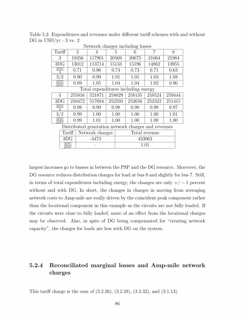
Table 5.2: Expenditures and revenues under different tariff schemes with and withoutDG in USD/yr - 3 vs. 2

Network charges including lossesTariff 3 4 5 6 7 8

3 18356 117901 20569 20675 21064 219843DG 13012 113714 15133 15196 14862 139553DG

30.71 0.96 0.74 0.73 0.71 0.63

3/2 0.90 0.99 1.01 1.01 1.03 1.083DG2DG

0.89 1.05 1.04 1.04 1.02 0.96Total expenditures including energy

3 255816 521871 258029 258135 258524 2594443DG 250472 517684 252593 252656 252322 2514153DG

30.98 0.99 0.98 0.98 0.98 0.97

3/2 0.99 1.00 1.00 1.00 1.00 1.013DG2DG

0.99 1.01 1.00 1.00 1.00 1.00

Distributed generation network charges and revenuesTariff Network charges Total revenue3DG -4473 4330633DG2DG

– 1.01

largest increases go to busses in between the PSP and the DG resource. Moreover, the

DG resource reduces distribution charges for load at bus 8 and slightly for bus 7. Still,

in terms of total expenditures including energy, the changes are only +/− 1 percent

without and with DG. In short, the changes in charges in moving from averaging

network costs to Amp-mile are really driven by the coincident peak component rather

than the locational component in this example as the circuits are not fully loaded. If

the circuits were close to fully loaded, more of an effect from the locational charges

may be observed. Also, in spite of DG being compensated for “creating network

capacity”, the charges for loads are less with DG on the system.

5.2.4 Reconciliated marginal losses and Amp-mile networkcharges

This tariff charge is the sum of (3.2.26), (3.2.28), (3.2.32), and (3.1.13).

86

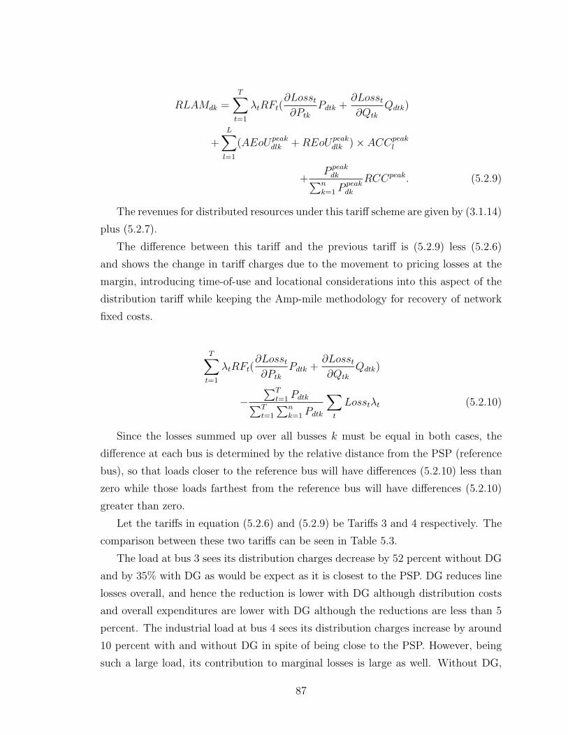
RLAMdk =T∑

t=1

λtRFt(∂Losst

∂Ptk

Pdtk +∂Losst

∂Qtk

Qdtk)

+L∑

l=1

(AEoUpeakdlk + REoUpeak

dlk )× ACCpeakl

+P peak

dk∑nk=1 P peak

dk

RCCpeak. (5.2.9)

The revenues for distributed resources under this tariff scheme are given by (3.1.14)

plus (5.2.7).

The difference between this tariff and the previous tariff is (5.2.9) less (5.2.6)

and shows the change in tariff charges due to the movement to pricing losses at the

margin, introducing time-of-use and locational considerations into this aspect of the

distribution tariff while keeping the Amp-mile methodology for recovery of network

fixed costs.

T∑t=1

λtRFt(∂Losst

∂Ptk

Pdtk +∂Losst

∂Qtk

Qdtk)

−∑T

t=1 Pdtk∑Tt=1

∑nk=1 Pdtk

∑t

Losstλt (5.2.10)

Since the losses summed up over all busses k must be equal in both cases, the

difference at each bus is determined by the relative distance from the PSP (reference

bus), so that loads closer to the reference bus will have differences (5.2.10) less than

zero while those loads farthest from the reference bus will have differences (5.2.10)

greater than zero.

Let the tariffs in equation (5.2.6) and (5.2.9) be Tariffs 3 and 4 respectively. The

comparison between these two tariffs can be seen in Table 5.3.

The load at bus 3 sees its distribution charges decrease by 52 percent without DG

and by 35% with DG as would be expect as it is closest to the PSP. DG reduces line

losses overall, and hence the reduction is lower with DG although distribution costs

and overall expenditures are lower with DG although the reductions are less than 5

percent. The industrial load at bus 4 sees its distribution charges increase by around

10 percent with and without DG in spite of being close to the PSP. However, being

such a large load, its contribution to marginal losses is large as well. Without DG,

87

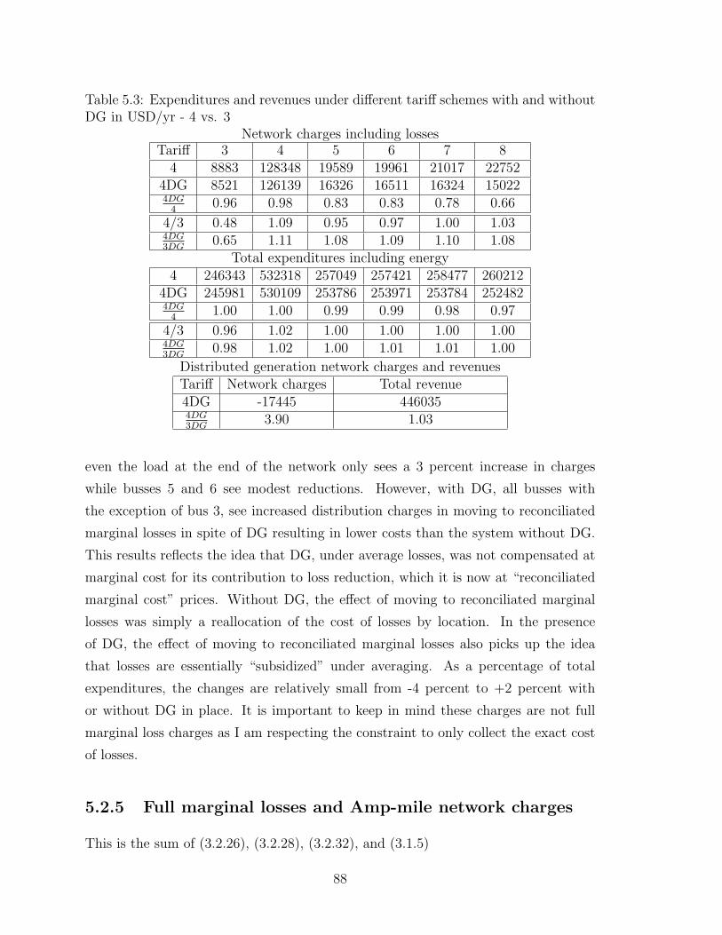
Table 5.3: Expenditures and revenues under different tariff schemes with and withoutDG in USD/yr - 4 vs. 3

Network charges including lossesTariff 3 4 5 6 7 8

4 8883 128348 19589 19961 21017 227524DG 8521 126139 16326 16511 16324 150224DG

40.96 0.98 0.83 0.83 0.78 0.66

4/3 0.48 1.09 0.95 0.97 1.00 1.034DG3DG

0.65 1.11 1.08 1.09 1.10 1.08Total expenditures including energy

4 246343 532318 257049 257421 258477 2602124DG 245981 530109 253786 253971 253784 2524824DG

41.00 1.00 0.99 0.99 0.98 0.97

4/3 0.96 1.02 1.00 1.00 1.00 1.004DG3DG

0.98 1.02 1.00 1.01 1.01 1.00

Distributed generation network charges and revenuesTariff Network charges Total revenue4DG -17445 4460354DG3DG

3.90 1.03

even the load at the end of the network only sees a 3 percent increase in charges

while busses 5 and 6 see modest reductions. However, with DG, all busses with

the exception of bus 3, see increased distribution charges in moving to reconciliated

marginal losses in spite of DG resulting in lower costs than the system without DG.

This results reflects the idea that DG, under average losses, was not compensated at

marginal cost for its contribution to loss reduction, which it is now at “reconciliated

marginal cost” prices. Without DG, the effect of moving to reconciliated marginal

losses was simply a reallocation of the cost of losses by location. In the presence

of DG, the effect of moving to reconciliated marginal losses also picks up the idea

that losses are essentially “subsidized” under averaging. As a percentage of total

expenditures, the changes are relatively small from -4 percent to +2 percent with

or without DG in place. It is important to keep in mind these charges are not full

marginal loss charges as I am respecting the constraint to only collect the exact cost

of losses.

5.2.5 Full marginal losses and Amp-mile network charges

This is the sum of (3.2.26), (3.2.28), (3.2.32), and (3.1.5)

88

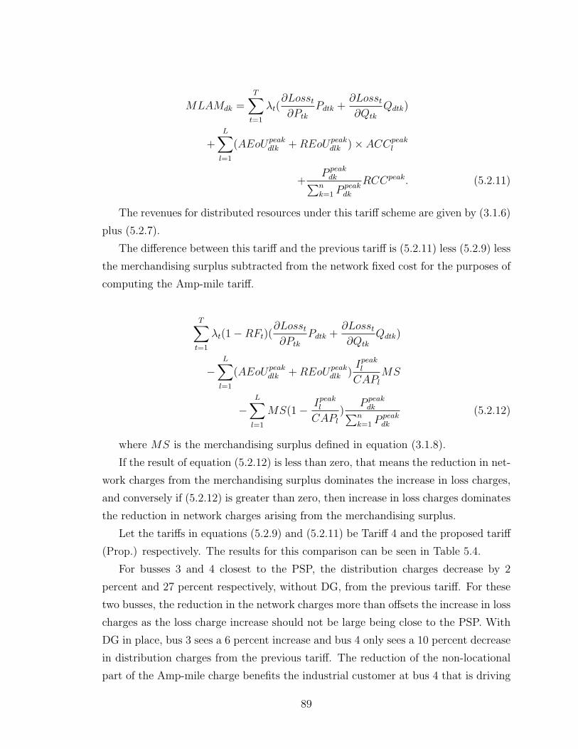
MLAMdk =T∑

t=1

λt(∂Losst

∂Ptk

Pdtk +∂Losst

∂Qtk

Qdtk)

+L∑

l=1

(AEoUpeakdlk + REoUpeak

dlk )× ACCpeakl

+P peak

dk∑nk=1 P peak

dk

RCCpeak. (5.2.11)

The revenues for distributed resources under this tariff scheme are given by (3.1.6)

plus (5.2.7).

The difference between this tariff and the previous tariff is (5.2.11) less (5.2.9) less

the merchandising surplus subtracted from the network fixed cost for the purposes of

computing the Amp-mile tariff.

T∑t=1

λt(1−RFt)(∂Losst

∂Ptk

Pdtk +∂Losst

∂Qtk

Qdtk)

−L∑

l=1

(AEoUpeakdlk + REoUpeak

dlk )Ipeakl

CAPl

MS

−L∑

l=1

MS(1− Ipeakl

CAPl

)P peak

dk∑nk=1 P peak

dk

(5.2.12)

where MS is the merchandising surplus defined in equation (3.1.8).

If the result of equation (5.2.12) is less than zero, that means the reduction in net-

work charges from the merchandising surplus dominates the increase in loss charges,

and conversely if (5.2.12) is greater than zero, then increase in loss charges dominates

the reduction in network charges arising from the merchandising surplus.

Let the tariffs in equations (5.2.9) and (5.2.11) be Tariff 4 and the proposed tariff

(Prop.) respectively. The results for this comparison can be seen in Table 5.4.

For busses 3 and 4 closest to the PSP, the distribution charges decrease by 2

percent and 27 percent respectively, without DG, from the previous tariff. For these

two busses, the reduction in the network charges more than offsets the increase in loss

charges as the loss charge increase should not be large being close to the PSP. With

DG in place, bus 3 sees a 6 percent increase and bus 4 only sees a 10 percent decrease

in distribution charges from the previous tariff. The reduction of the non-locational

part of the Amp-mile charge benefits the industrial customer at bus 4 that is driving

89

Table 5.4: Expenditures and revenues under different tariff schemes with and withoutDG in USD/yr - Proposed vs. 4

Network charges including lossesTariff 3 4 5 6 7 8Prop 8724 93600 27815 28421 29976 31980

PropDG 8996 113329 22454 22762 22871 21474PropDG

Prop1.03 1.21 0.81 0.80 0.76 0.67

Prop/4 0.98 0.73 1.42 1.42 1.43 1.41PropDG

4DG1.06 0.90 1.38 1.38 1.40 1.43

Total expenditures including energyProp 246184 497570 265275 265881 267436 269440

PropDG 246456 517299 259914 260222 260331 258934PropDG

Prop1.00 1.04 0.98 0.98 0.97 0.96

Prop./4 1.00 0.93 1.03 1.03 1.03 1.04Prop.4DG

1.00 0.98 1.02 1.02 1.03 1.03

Distributed generation network charges and revenuesTariff Network charges Total revenue

PropDG -30506 459096PropDG

4DG1.75 1.03

the peak. The presence of DG reduces losses and loading and hence reduces the

merchandising surplus under full nodal pricing so the amount of rebate the industrial

customer at bus 4 and the load at bus 3 can receive is less. For the remaining busses,

the distribution charges increase between 38 percent and 43 percent driven by their

distance from the PSP, and their low contribution to system peak that results in a

low “rebate” from the merchandising surplus. Still, in spite of the large percentage

changes in distribution charges, the overall change in energy charges ranges from -7

to +4 percent without DG and a range of -2 to +3 percent with DG.

5.2.6 Benchmark average cost tariff vs. proposed cost cau-sation based tariff

Having looked at the decomposition of the tariff changes, the complete change in

moving from the average cost tariff to the proposed cost-causation based tariff is

examined in Table 5.5. On observation is that even residential loads far from PSP see

a decrease in distribution tariff charges moving toward the nodal pricing, Amp-mile

method whether or not DG is present in the system, though the decreases are larger

with DG in the system than without it. This is a counterintuitive result in that

90

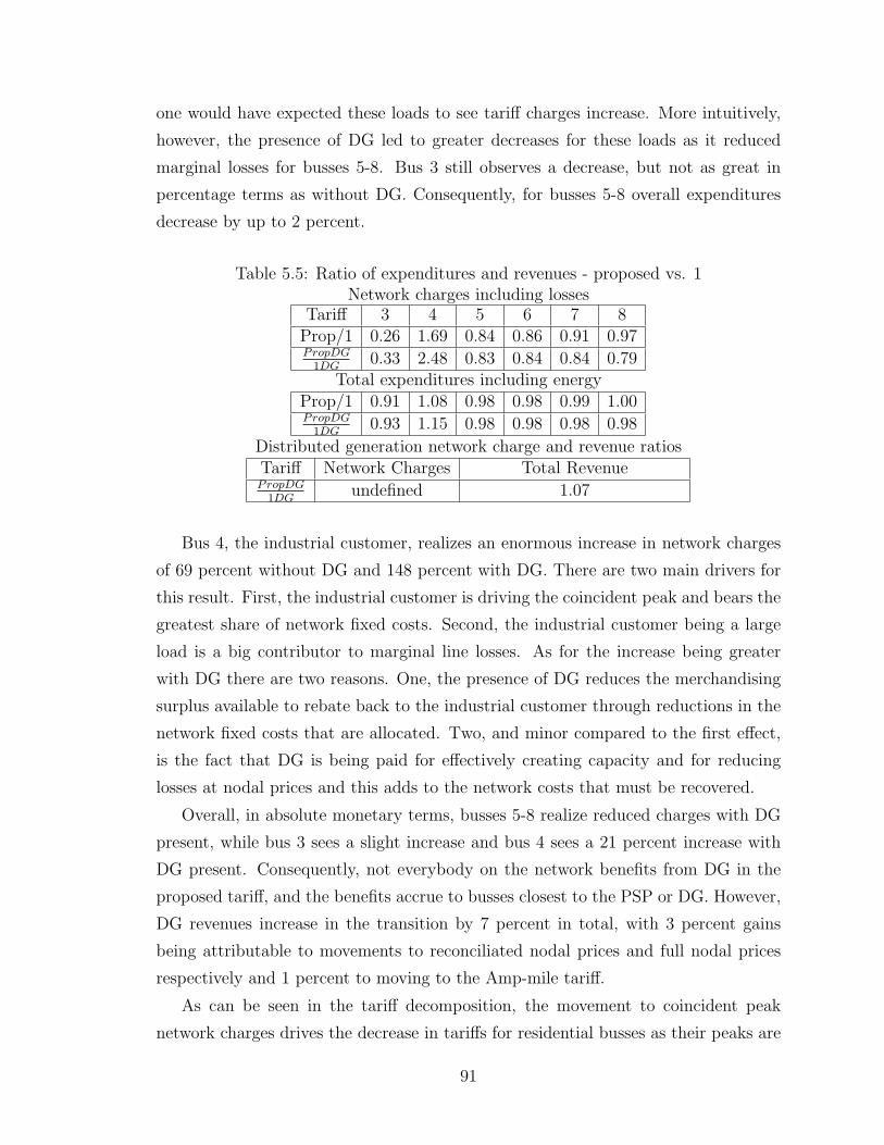
one would have expected these loads to see tariff charges increase. More intuitively,

however, the presence of DG led to greater decreases for these loads as it reduced

marginal losses for busses 5-8. Bus 3 still observes a decrease, but not as great in

percentage terms as without DG. Consequently, for busses 5-8 overall expenditures

decrease by up to 2 percent.

Table 5.5: Ratio of expenditures and revenues - proposed vs. 1Network charges including losses

Tariff 3 4 5 6 7 8Prop/1 0.26 1.69 0.84 0.86 0.91 0.97PropDG

1DG0.33 2.48 0.83 0.84 0.84 0.79

Total expenditures including energyProp/1 0.91 1.08 0.98 0.98 0.99 1.00PropDG

1DG0.93 1.15 0.98 0.98 0.98 0.98

Distributed generation network charge and revenue ratiosTariff Network Charges Total RevenuePropDG

1DGundefined 1.07

Bus 4, the industrial customer, realizes an enormous increase in network charges

of 69 percent without DG and 148 percent with DG. There are two main drivers for

this result. First, the industrial customer is driving the coincident peak and bears the

greatest share of network fixed costs. Second, the industrial customer being a large

load is a big contributor to marginal line losses. As for the increase being greater

with DG there are two reasons. One, the presence of DG reduces the merchandising

surplus available to rebate back to the industrial customer through reductions in the

network fixed costs that are allocated. Two, and minor compared to the first effect,

is the fact that DG is being paid for effectively creating capacity and for reducing

losses at nodal prices and this adds to the network costs that must be recovered.

Overall, in absolute monetary terms, busses 5-8 realize reduced charges with DG

present, while bus 3 sees a slight increase and bus 4 sees a 21 percent increase with

DG present. Consequently, not everybody on the network benefits from DG in the

proposed tariff, and the benefits accrue to busses closest to the PSP or DG. However,

DG revenues increase in the transition by 7 percent in total, with 3 percent gains

being attributable to movements to reconciliated nodal prices and full nodal prices

respectively and 1 percent to moving to the Amp-mile tariff.

As can be seen in the tariff decomposition, the movement to coincident peak

network charges drives the decrease in tariffs for residential busses as their peaks are

91

counter-cyclic to the coincident peak and contribute relatively little to the coincident

peak. By the same token, the industrial customer drives the peak and its tariff increase

is driven by the move toward coincident peak network charges. The locational aspects

have only a small effect in relative terms surprisingly. This may be different if the

network is close to fully loaded at peak.

With respect to losses, the movement to full marginal losses under nodal pricing

has an offsetting effect from the movement to coincident peak network charges and

the two are intimately linked. Full marginal losses leads to charges that are higher

the farther away from the PSP, all else equal. Moreover, there is a merchandising

surplus from using full marginal losses that can be used to offset the network charges

for everybody in the proposed methodology. And because the industrial customer is

driving the coincident peak, it will also benefit most from the use of the merchandising

surplus to offset the network charges. Hence, the overall decrease to busses 5-8 is

dampened by full marginal losses under nodal pricing and the overall increase to the

industrial customer is dampened by the use of full marginal losses.

5.3 Chapter Concluding Remarks

In this chapter a decomposition of the changes in distribution tariff charges in moving

from a purely average cost tariff structure to a cost-causation based tariff structure

with full marginal losses and an extent-of-use (Amp-mile) method for the recovery of

network fixed costs with and without the presence of controllable distributed genera-

tion has been shown. Decomposing the tariff changes is important to understanding

why charges have changed in the way they have so that seemingly counter-intuitive

results can be understood. In the case study, the big drivers for the change in tariff

charges are the changes due to moving to coincident peak charges for network cost

allocation and moving to full nodal pricing for the recovery of losses. Consequently,

both time and locational aspects are important. The counter-intuitive results were

that residential loads far from the PSP saw their charges decrease, and industrial load

closer to the PSP saw its charges increase substantially. More intuitively, the charges

of the industrial customer should rise as it is driving the coincident peak whereas the

residential peaks are countercyclical to the coincident peak and it is this result that

dominates the locational result. The results would look different under different load

profiles and topologies.

DG adds nuances to the analyzed effects. With respect to moving to reconciliated

92

marginal losses, DG exposes the idea that paying for losses at higher prices shows how

load is being “subsidized” under loss averaging. Moreover, DG increases the network

fixed costs that must be recovered as it effectively creates network capacity. DG also

reduces line losses overall and thus reduces the merchandising surplus that can be

rebated back to load by offsetting network fixed cost. Finally, DG, while benefiting

those closest to it, seems to increase network charges for some loads on the network.

It is important to note in the final analysis that the effects of tariff changes in the

presence of DG may change considerably with different load profiles and different

topologies.

93

94

Chapter 6

General Conclusions and Results

Traditional cost allocation methodologies such as averaging do not provide adequate

incentives for the deployment of DG as no consideration is given for the ability of DG

to reduce the network use or losses. Rather than viewing DG pricing as a distribution

network pricing problem, most countries which are aware of the potential benefits of

DG adopt specific ad-hoc policies which subsidize DG.

In this research, it has been proposed to use cause-causality based tariffs for dis-

tribution networks to enhance DG revenue without using ad-hoc policies or subsidies.

As the distribution network becomes an active network, similar to transmission, tra-

ditional pricing schemes need to be adapted or changed. Although there is little

literature existing regarding cost reflective or usage based tariffs for distribution,

there is a lot of work and experience for the case of transmission. Except for the work

of (Mutale et al., 2000), (Costa P. and Matos, M., 2004) or (De Oliveira et al., 2004),

which assess the problem of allocation of network losses for distribution networks with

DG, nothing is found with respect to new methods for allocation of fixed costs at the

distribution level.

The proposed tariff scheme for distribution networks with DG is based on two

concepts:

1. The use of nodal pricing for distribution networks, which allocates losses in an

efficient manner.

2. The design of a particular “extent of use” method for the allocation of fixed

network costs.

With respect to the allocation of fixed network costs, the Amp-mile method,

inspired by the well known MW-mile methods used for transmission, but adapted

95

to distribution networks (i.e., using current flows instead of power flows) has been

proposed. The method proves to have the following features:

• It is cost reflective or usage based in the sense that network users (e.g. loads

and generators) pays accordingly to their extent-of-use of the network.

• It explicitly accounts for flow direction rewarding potential DG units that free

up, or in effect, create additional distribution network capacity.

• For the case of load, demand customers who impose a low network use have

lower charges than those which impose high network use.

• The price signals sent become stronger as network utilization increases; in par-

ticular, if the network were fully loaded all fixed costs would be recovered by

the locational charges.

• The resulting charges give price signals with respect to the operation and siting

of DG and loads.

Simulating the use of Amp-mile tariffs within a distribution network similar to

one that can be found in Uruguay, it was found that overall, for the case without DG,

the locational charges recover 18 percent of the network fixed cost while the other 82

percent is recovered by the non-locational charges. With DG, as it reduces network

loading, the amount recovered by locational charges is reduced to only 12 percent.

As the simulation show, the more the network is loaded, the greater is the amount

recovered by the locational component of the tariff. Moreover, both for the case of

time differentiated, per unit locational charges or fixed, coincident peak locational

charges within Amp-mile, without DG, customers with the same load profiles (e.g.

residential) pay more the farther away they are from the PSP. In particular, demand

customers at node 3 benefit from being closer to the PSP as they have lower network

use, while demand customers at node 8 are charged more for having higher network

use. However, with DG installed at node 8, as the power flows in circuits 6-7 and 7-8

are reversed, demand customers at bus 8 have lower network use than in the previous

case without DG, and thus pay lower Amp-mile charges. In all the simulated cases,

DG receives payments from Amp-mile tariffs in recognition for essentially creating

extra capacity in the network. In addition, these payments are greater the more

hours the DG is running, varying from $62/yr for the case of wind DG with 0.20

capacity factor to $2696/yr for the case of controllable DG.

96

With respect to the allocation of losses, it has been proposed to use nodal pricing

which has the following properties:

• Nodal pricing is an economically efficient pricing mechanism for short term

operation that has been used worldwide for transmission systems.

• Nodal prices give the right signals for location and operation of both demand

and generation

• Under nodal pricing distributed generators / loads are paid / charged the nodal

price including marginal losses.

• The distribution company recovers the energy costs inclusive of losses plus a

merchandising surplus that, in general, is greater than zero. This amount can

be used to offset the total fixed network costs, which provides a lower cost base

from which to apply the Amp-mile charges.

• Using the merchandising surplus from nodal pricing to offset the fixed costs

used in the Amp-mile method does not dampen the locational price signal. The

locational signal is strengthened since network fixed costs are recovered through

locational signals via the merchandising surplus resulting from nodal prices and

through the locational signal from the Amp-mile tariff on the remaining fixed

costs.

When simulating nodal prices in the specific case study network it was found that,

depending on load, these prices can differ quite significantly from the PSP prices. For

instance, without DG, in winter, at node 8 (which is far away from the PSP), nodal

active prices reach values of above $92/MWh, while the PSP price is $76/MWh. This

reflects the high impact on network losses of demand customers at node 8. In addition,

for the same season and time, and also without DG, values of nodal prices at node

4 are less than $92/MWh, because node 4 is closer to the PSP. Without DG, prices

increase with the distance to the PSP. This means that demand customers far away

from the PSP must pay higher electricity prices, because they impose higher network

losses. Similar results can be observed for nodal reactive prices. The graphs showed

that nodal prices follow the load profile curve, being greater at times of higher network

loading and smaller at times of lower network loading. Once again, demand customers

must pay higher electricity prices at times of higher network loading, not only because

it price are higher at higher load levels, but also because they are imposing greater

97

losses. As a result, at peak times, the incentives for demand customers are to reduce

loading, while the incentives for a DG resource is to increase production. With nodal

prices controllable DG receives $456400 per year instead of the $428590 obtained

with PSP prices, representing 6.5 percent increase in revenues. In the case study,

the effect of controllable DG in the network was to reduce losses and thus to reduce

nodal prices. The merchandising surplus decreases from $101740 for the case without

DG, to $53478 with controllable DG, with decreasing values for intermittent DG of

increasing capacity factors. Since the merchandising surplus is used for offsetting fixed

network charges, reduced values of merchandising surplus leads to more of the fixed

network cost being allocated through the Amp-mile method. However, it was found

that total charges collected from loads decrease as the DG capacity factor increases.

This decrease (of less than 0.5 percent for controllable DG) takes place as the total

fixed network costs are increasing due to payments to DG for freeing up network.

The proposed tariff scheme (i.e., nodal pricing plus Amp-mile) is analyzed relative

to traditional pro-rata methodologies to show the difference in DG revenue, tariff

expenditures, and decomposition of tariff and revenue changes.

• For this particular case, controllable DG receives 7 percent more income, which

takes into account both the effects of reduced losses and network use. These

revenues reflect cost causality and can offset subsidies that have been used to

promote DG.

• With regard to intermittent wind DG, contributions to loss reductions and

network use are not as great in expectation as it contributes little to counter

flows at peak time, when the extent of use and losses are greatest.

• Examination of the decomposition of the changes in distribution tariff charges

in moving from a purely average cost tariff structure to a cost-causation based

tariff structure with full marginal losses and the Amp-mile method for the re-

covery of network fixed cost, it can be seen that the big drivers for the change

are the changes due to moving to coincident peak charges for network cost allo-

cation and moving to full nodal pricing for the recovery of losses. Although the

result is dependant on the particular network characteristics (i.e., topology, load

profiles and generation pattern), in general, both time and locational aspects of

generation and consumption are important.

98

It seems to be clear that without cost reflective tariffs at distribution level, there

is little hope of inducing DG resources to locate and operate so they can provide the

system benefits as shown in previous chapters. Given worldwide experience with nodal

pricing and extent-of-use methods for fixed cost allocation at transmission level, and

the fact that DG resources transform the distribution network into an active network

like transmission, it makes sense to consider these methodologies in distribution.

Finally, there is much more work to do regarding the pricing of DG. Apart from

the potential benefits of DG that are recognized in the proposed tariffs within this

research (i.e. reduce in network use and losses), DG has the potential to provide

ancillary services in the distribution network, such as voltage control or capacity

reserve. These services need also to be efficiently priced and should be considered

and studied in future research. In addition, for renewable DG, there is the potential

to reduce emissions, and this characteristic should also be properly recognized and

rewarded.

99

100

Bibliography

Baldick, R. (2003). Variations of Distribution Factors with Loading. IEEE Transac-

tions on Power Systems, Vol. 18, No4, pp. 1316-1323.

Bernstein, J.S. (1999). Regulacion en el Sector Distribucion Electrica. Tesis presen-

tada en la Pontificia Universidad Catolica de Chile, Escuela de Ingenierıa, Dpto.

Ingenierıa Electrica.

Bialek, J. (1998). Allocation of Transmission Supplementary Charge to Real and

Reactive Loads. IEEE Transactions on Power Systems, Vol. 13, No3, pp. 749-

754.

Bialek, J. 1/97 (1997). Elimination of merchandise surplus due to spot pricing of

electricity. IEE Proc.-Gener.Transm.Distrib., Vol. 144, No5, September 1997.

Bialek, J. 2/97. (1997). Topological Generation and Load Dispatch Factors for Sup-

plement Charge Allocation in Transmission Open Access. IEEE Transactions on

Power Systems, Vol. 12, No3, pp. 1185-1194.

Bitrain, E. and Saavedra, E. 1/93 (1993). Rol Regulador y Empresarial del Estado.

Publicacion dentro de Hacia el Estado Regulador, Oscar Munoz, CIEPLAN.

Bitrain, E. and Saavedra, E. 2/93 (1993). La regulacion del sector electrico: la expe-

riencia chilena. Publicacion dentro de Hacia el Estado Regulador, Oscar Munoz,

CIEPLAN.

CIGRE (1999). Working Group 37.23. Impact of Increasing Contribution of Dispersed

Generation on Power System.

CIRED (1999). Working Group 4. Preliminary Report Discussion at CIRED 1999,

Nice, France, 2nd June.

101

Costa, P. and Matos, M. (2004). Loss Allocation in Distribution Networks with

Embedded Generation. IEEE Transactions on Power Systems, Vol. 19, No1, Feb.

2004, pp. 384-389.

Chu, W.C., Chen, B.K., Hsu, N.S. (2001). The Economic Dispatch With Considera-

tion of Transmission Service Charge for a Generation Company. IEEE Transac-

tions on Power Systems, Vol. 16, No4, 2001, pp. 737-742.

De Oliveira, M., Ochoa, L., Padilha-Feltrin, A and Mantovani, J. (2004). Network

Reconfiguration and Loss Allocation for Distribution Systems with Distributed

Generation. Proceedings Latin America IEEE T & D 2004, No079, Sao Paulo,

Brazil.

Dunsky, P. (2000). Cogeneration and On-Site Power Production. COSPP, Issue 6.

Foster, V. and Antmann, P. (2004). The Regulatory Challenge of Asset Valu-

ation. A Case Study from the Brazilian Electricity Distribution Sector. The

World Bank Group, Energy Working Notes, Energy and Mining Sector Board,

found at http://siteresources.worldbank.org/INTENERGY/Resources/335544-

1111615897422/EnergyWorkingNotes2.pdf

Ghosh, S. and Das, D. (1999). Method for load-flow solution of radial distribution

networks. IEE Proc.-Gener.Transm.Distrib.,Vol. 146, No6, November 1999, pp.

641-648.

Hadley, S.W., Van Dyke, J.W., Stovall, T.K. (2003). The Effect of Distributed Energy

Resource Competition with Central Generation. ORNL/TM-2003/236, Depart-

ment of Energy, Office of Energy Efficiency and Renewable Energy, Oak Ridge

National Laboratory, October 2003.

Hogan, W.W. (1998). Nodes and Zones in Electricity Markets: Seeking Simplified

Congestion Pricing in Designing Competitive Electricity Market. Hung-po Chao

and Hillard G. Huntington, editors.

Hunt, S. and Shuttleworth, G. (1996). Competition and Choice in Electricity. John

Wiley & Sons.

Hyde, D. (1998). Will Consumers Choose Renewable Energy, and Should You Care

One Way or the Other. IEEE Power Engineering Review.

102

Ianucci, J.J., Cibulka, L., Eyer, J.M., and Pupp, R.L. (2003). DER Benefits Analysis

Study: Final Report, NREL/SR-620-34636. National Renewable Energy Labora-

tory, September 2003.

International Energy Agency (2002). Distributed Generation in Liberalised Electricity

Markets. OECD/IEA Publications, Paris, France.

Jenkins, N. et al. (2000). Embedded Generation. IEE Power and Energy Series 31,

ISBN 0 85296 774 8.

Kovacs, R.R. and Leverett, A.L. (1994). A Load Flow Based Method for Calculating

Embedded, Incremental, and Marginal Cost of Transmission Capacity. IEEE

Transactions on Power Systems, Vol. 9, No1, pp. 272-278.

Maranagon Lima, J.W. (1996). Allocation of Transmission Fixed Charges: An

Overview. IEEE Transactions on Power Systems. Vol. 11, No3, pp. 1409-1418,

August 1996.

Maranagon Lima, J.W., Pereira, M.V.F. and Pereira, J.L.R. (1996). An Integrated

Framework for Cost Allocation in a Multi-Owned Transmission System. IEEE

Transactions on Power Systems. Vol. 10, No2, pp. 971-977, May 1996.

Mendez, V.H., Rivier, J., De la Fuente, J.I., Gomez, T., Areceluz, J., Marin, J. (2002).

Impact of Distributed Generation on Distribution Losses. Universidad Pontificia

Comillas, found at www.iit.upcomillas.es/docs/02VMQ01.pdf, November 2002.

Mutale, J., Strbac, G., Curcic, S. and Jenkins, N. (2000). Allocation of losses in distri-

bution systems with embedded generation. IEE Proc.-Gener. Transm. Distrib.,

147(1), pp. 1-8.

Nemhauser, G.L., Rinnoy Kay, A.H.G., Todd, M.J.(eds.) (2000). Handbooks in Oper-

ation Research and Management Science. Vol. 1, Optimization, North Holland.

OFGEM (2005). Structure of electricity distribution charges. Consultation on the

longer term charging framework, found at http://www.ofgem.gov.uk.

Pan, J., Teklu, Y., Rahman, S., and Jun, K. (2000). Review of Usage-Based Trans-

mission Cost Allocation Methods under Open Access. IEEE Transactions on

Power Systems, Vol. 15, No4, 2000, pp. 1218-1224.

103

Park, Y.M., Park, J.B., Lim, J.U. and Won, J.R. (1998). An Analytical Approach

for Transaction Cost Allocation in Transmission Systems. IEEE Transactions on

Power Systems, Vol. 13, No4, 1998, pp. 1407-1412.

Pereira da Silva, J., Saraiva, J.T. and Ponce de Leao, M.T. (2001). Use of Power

Flow Based Embedded Methods to Set Tariffs for Use of Networks - A Case

Study Using the Portuguese Transmission System. Presented at 2001 IEEE Porto

Power Tech Conference, 10-13 September, 2001, Porto, Portugal.

Perez-Arriaga, I.J. and Smeers, Y. (2003). Guidelines on Tariff Setting in Transport

Pricing of Electricity Networks. Francois Leveque, editor.

Perez-Arriaga, I.J., Rubio, F.J., Puerta, J.F., Arceluz, J., Marın, J. (1995). Marginal

Pricing of Transmission Services: An Analysis of Cost Recovery. IEEE Transac-

tions on Power Systems, Vol. 10, No1, pp. 546-553.

Programa de Desarrollo Tecnologico (PDT) - Facultad de Ingenierıa (2006).

Proyecto PDT S/C/OP/16/04: Generacion distribuida en el Uruguay: Eval-

uacion de fortalezas, oportunidades y tratamiento regulatorio, found at

http://iie.fing.edu.uy/investigacion/grupos/gd/informefinalcompleto.pdf

Poder Ejecutivo de Uruguay (2002). Reglamento de Distribucion de Energıa Electrica,

Decreto No277/02.

Regulatory Assistance Project (RAP). (2001). Expected Emissions

Output from Various Distributed Energy Technologies, found at

http://www.raponline.org/ProjDocs/DREmsRul/Collfile/

DGEmissionsMay2001.pdf.

Rubio-Odriz, F.J. and Perez-Arriaga, I.J. (2001). Marginal Pricing of Transmission

Services: A Comparative Analysis of Network Cost Allocation Models. IEEE

Transactions on Power Systems, Vol. 15, No1, pp. 448-454.

Rudnick, H., Palma, R., Fernandez, J.E. (1995). Marginal Pricing and Supplement

Cost Allocation in Transmission Open Access. IEEE Transactions on Power

Systems, Vol. 10, No2, pp. 1125-1132.

Schweppe, F.C., Caramanis, M.C., Tabors, R.D. and Bohn, R.E. (1988). Spot Pricing

of Electricity.

104

Shirmohammadi, D., Gribik, P.R., Law, E.T.K., Malinowski, J.H. and O’Donnell,

R.E. (1989). Evaluation of Transmission Network Capacity Use for Wheeling

Transactions. IEEE Transactions on Power Systems, Vol. 4, No4, pp. 1405-1413.

Sotkiewicz, P.M. and Vignolo, J.M. 1/07 (2007). Towards a Cost Causation-Based

Tariff for Distribution Networks with DG. IEEE Transactions on Power Systems,

Vol. 22, No3, August 2007, pp. 1051-1060.

Sotkiewicz, P.M. and Vignolo, J.M. 2/07 (2007). Distributed Generation. The Ency-

clopedia of Engineering and Technology, Ed. Barney Capehart, New York, Taylor

and Francis, July 2007.

Sotkiewicz, P.M. and Vignolo, J.M. 1/06 (2006). Nodal Prices for Distribution Net-

works: Efficient Pricing for Efficiency DG Enhancing. Letters to IEEE Transac-

tions on Power Systems, Vol. 21, No2, May 2006.

Sotkiewicz, P.M. and Vignolo, J.M. 2/06 (2006). Allocation of Fixed Costs in Dis-

tribution Networks with Distributed Generation. IEEE Transactions on Power

Systems, Vol. 21, No2, May 2006.

Sotkiewicz, Paul M. (2006). Nodal Pricing and MW-mile Methods for Distribution:

Have We Uncovered Markets or Elements for Wholesale Markets. Presentation

at the Harvard Electricity Policy Group 42nd Plenary Session, March 2, 2006,

La Jolla, CA. Found at www.ksg.harvard.edu/hepg

Su, C.T. and Liaw, J.H. (2001). Power Wheeling Pricing Using Power Tracing and

MVA-KM Method, presented at 2001 IEEE Porto Power Tech Conference, 10-13

September, 2001, Porto, Portugal.

United States Department of Energy (USDOE) (2007). Annual Report on U.S.

Wind Power Installation, Cost, and Performance. Trends: 2006, found at

http://www.eere1.energy.gov/windandhydro/pdfs/41435.pdf

United States Energy Information Administration (USEIA) 1/07 (2007).

Annual Energy Outlook 2007 with Projections to 2030, found at

http://www.eia.doe.gov/oiaf/aeo/pdf/trend 4.pdf.

United States Energy Information Administration (USEIA) 2/07 (2007). Gasoline and

Diesel Fuel Update and Spot Prices, found at http://www.tonto.eia.doe.gov.

105

Vignolo, J.M. (2002). The Influence of Market Regulations in the Development of

Distributed Generation. Proceedings of the 2nd International Symposium on Dis-

tributed Generation, Estocolmo, Suecia, 2002.

Vignolo, J.M. and Zeballos, R. (2001). Transmission Networks or Distributed Gen-

eration? Proceedings of the Sixth IASTED International Conference on Power

and Energy Systems, Rodas, Grecia, Junio, 2001.

Vignolo, J.M. and Zeballos, R. (2000). La Generacion Distribuida en el Mercado

Electrico Uruguayo, Encuentro Camara de Industrias del Uruguay.

World Alliance for Decentralized Energy (WADE) (2006).

World Survey of Decentralized Energy 2006, found at

http://www.localpower.org/documents pub/report worldsurvey06.pdf

World Alliance for Decentralized Energy (WADE) (2003). WADE

Guide to DE Technologies - Cogeneration Technologies, found at

http://www.localpower.org/documents pub/report de technologies.pdf

Williams, P. and Strbac, G. (2001). Costing and pricing of electricity distribution

services. Power Engineering Journal, Electricity Distribution, 125-136.

Willis, H. Lee and Scott, Walter G. (2000). Distributed Power Generation. Planning

and Evaluation. Marcel Dekker, Inc., ISBN 0-8247-0336-7.

106

Appendix A

Power Flow and AnalyticalDerivatives Calculation1

The equations for the power flow are:

i(k) =∑

h∈Hink

f(h)−∑

h∈Houtk

f(h),∀k ∈ V (A.0.1)

v(k)conj(i(k)) = s(k) = p(k) + jq(k), ∀k ∈ V (A.0.2)

v(kh,ini)− v(kh,end) = (r(h) + jx(h))f(h), ∀h ∈ E (A.0.3)

where,

i(k), is the complex charging current for node k

f(h), is the complex current flowing through line h

v(k), is the complex voltage at node k

conj(z), is the conjugate of complex number z

s(k), is the loading apparent power at node k, being p(k), q(k), the active and

reactive power respectively; p(k), q(k) > 0 corresponds to consumption/demand,

p(k), q(k) < 0 corresponds to generation

r(h), x(h), are the resistance and the reactance for line h

H ink , Hout

k are the sets of entry lines and salient lines for node k, respectively

V , is the set of nodes

E, is the set of lines

1This power flow was developed with the assistance of MSc. Ing. Alfredo Piria.

107

Equation A.0.1 corresponds to the current balance at each node, equation A.0.2

is the definition of the apparent power for each node relating voltage, current and

power and equation A.0.3 is Ohms law applied to each line. Note that all magnitudes

are in per unit.

For the case we are studying our unknown variables are v and i while the known

variables are all ps and qs. The only exception to this is the voltage at the slack bus,

which is known and set at 1 p.u..

We will work with the matricial form of equations A.0.1, A.0.2, A.0.3:

i = AT f (A.0.4)

v. ∗ conj(i) = p + jq (A.0.5)

Av = −(r + jx). ∗ f (A.0.6)

where A es the incident matrix lines-nodes defined as follows:

A/

A(h, kh,end) = 1

A(h, kh,ini) = −1

A(h, k) = 0∀k 6= kh,ini, kh,end

(A.0.7)

The notation .∗ indicates the operation element by element.

For our particular case where the network is radial we have nnod = nlines+1 and the

slack bus ks is the PSP, where the distribution network connects to the transmission

network.

Let us call Vns the set of nodes different from the slack bus, then V = ks ∪ Vns.

We will use a similar notation for vectors v, i and for matrix A:

v = (vs, vns); i = (is, ins); A = (As, Ans)

where vs = v0 is known, As is the column ks of A and Ans is a square matrix

obtained from withdrawing the column ks of A. It is possible to prove that Ans is

invertible; we are not going to do so here.

Then equations A.0.4, A.0.5, A.0.6 can be written as follows:

108

is = ATs f (A.0.8)

ins = ATnsf (A.0.9)

v0conj(is) = ps + jqs (A.0.10)

vns. ∗ conj(ins) = pns + jqns (A.0.11)

Asv0 + Ansvns = −Rf (A.0.12)

where R is a diagonal matrix with vector r + jx at the diagonal. In order to

find vns, ins, f we can focus in the resolution of equations A.0.9, A.0.11 and A.0.12.

Afterwards equations A.0.8 and A.0.10 allow us to calculate the current and the power

at the slack bus once fluxes f through the lines are known. Let us call,

A2 =(AT

ns

)−1

We can then calculate f from A.0.9 obtaining:

f = A2ins (A.0.13)

Then substituting in A.0.12 we have:

Asv0 + Ansvns = −RA2ins

and then,

vns = A−1ns (−Asv0 −RA2ins)

vns = −v0AT2 As − AT

2 RA2ins

vns = d + Dins (A.0.14)

where,

d = −v0AT2 As is a column vector of nline elements

109

D = −AT2 RA2 is a square matrix of size nline.

To sum up, we have to solve a non linear system of equations consisting in equa-

tions A.0.11 and A.0.14, which may be written as:

ins = (pns − jqns)./conj(vns) (A.0.15)

vns = d + Dins (A.0.16)

The advantage of this reasoning is that allows to calculate the currents from the

voltages and viceversa in a form that is adequate to an iterative algorithm.

A.0.1 The iterative algorithm

The iterative algorithm used is as follows:

First step: Choose tolerance ε and set v(k) = v0∀k ∈ Vns

Iterative step:

1) Save in vold the actual value of voltage vector vns

2) Calculate the current vector ins using A.0.15

3) Calculate the voltage vector vns using A.0.16

4) If ‖vns − vold‖ < ε, the iteration is finished. In other case, go to 1).

Final step: Calculate f using A.0.13, then is using A.0.8, and active and reactive

powers ps, qs using A.0.10.

The convergence of the method can be proven in a similar way as it is done in

(Ghosh, S. and Das, D., 1999). It can be proven a linear convergence, corresponding

to the limit: limiter→∞

‖viter+1−v∗‖‖viter−v∗‖ < β , with β < 10−2.

In practice, it can be observed a fast convergence, reaching a tolerance of 10−6 in

vector v within an average of 6 iterations.

A.0.2 Derivatives calculation

Derivatives of node currents with respect to loading active and reactivepowers

From equations A.0.11 and A.0.16 which relate current, voltage and active and

reactive powers at network nodes:

110

conj(ins). ∗ vns = pns + jqns

vns = d + Dins

we obtain the node loading power as a function of the node loading current:

sns = pns + jqns = F (ins) = conj(ins). ∗ (d + Dins) (A.0.17)

The idea is to find the matrix derivatives of powers with respect to currents and

then calculate the inverse.

To do this, we firstly make a distinction between the real and imaginary parts of

the complex magnitudes:

ins = z + jy, D = D1 + jD2

Then substituting in equation A.0.17 we obtain two real functions:

pns = F1(z, y)

qns = F2(z, y)

pns = z. ∗ (d + D1z −D2y) + y. ∗ (D2z + D1y) (A.0.18)

qns = −y. ∗ (d + D1z −D2y) + z. ∗ (D2z + D1y) (A.0.19)

In order to find the matrix of partial derivatives, we will see at first how the

Jacobian matrix ∂f∂x

of a vectorial function f : RN → RN defined as f(x) = u(x).∗v(x)

looks like.

As fk(x) = uk(x)vk(x), ∂fk(x)∂xh

= ∂uk(x)∂xh

vk(x)+uk(x)∂vk(x)∂xh

. Then row k of ∂f∂x

matrix

is∂fk

∂x= vk

∂uk

∂x+ uk

∂vk

∂x

and then:

∂f

∂x= diag(v)

∂u

∂x+ diag(u)

∂v

∂x(A.0.20)

As a result, applying A.0.20 to our functions in A.0.18 and A.0.19, we have:

111

∂F1

∂z= diag(z)D1 + diag(y)D2 + diag(d + D1z −D2y) (A.0.21)

∂F1

∂y= −diag(z)D2 + diag(y)D1 + diag(D2z + D1y) (A.0.22)

∂F2

∂z= diag(z)D2 − diag(y)D1 + diag(D1z + D2y) (A.0.23)

∂F2

∂y= diag(z)D1 + diag(y)D2 − diag(d + D1z −D2y) (A.0.24)

The desired Jacobian matrices are then:

J0 =∂(pnr, qnr)

∂(z, y)=

(∂F1

∂z∂F1

∂y

∂F2

∂z∂F2

∂y

)

and

J1 =∂(z, y)

∂(pnr, qnr)=

(∂F1

∂z∂F1

∂y

∂F2

∂z∂F2

∂y

)−1

(A.0.25)

Derivatives of the line currents with respect to node currents

From equation A.0.13, and including notation f = f1 + jf2, we have that f1 + jf2 =(AT

ns

)−1(z + jy) and then:

∂f1

∂z=

∂f2

∂y=

(AT

ns

)−1,∂f1

∂y=

∂f2

∂z= 0

Finally, the Jacobian matrix is:

J2 =

(∂f1

∂z∂f1

∂y

∂f2

∂z∂f2

∂y

)=

( (AT

ns

)−10

0(AT

ns

)−1

)(A.0.26)

Derivatives of absolute values of line currents with respect to node activeand reactive powers

We would like to calculate the Jacobian matrix J6 = ∂I∂(pns,qns)

with the partial deriva-

tives of absolute values I(h) = abs (f(h)) =√

f1(h)2 + f2(h)2 of the line currents

with respect to the active and reactive powers at nodes (except the slack).

112

We have already calculated matrix J2 = ∂(f1,f2)∂(z,y)

with the derivatives of the line

currents with respect to node currents ins = z + jy, and matrix J1 = ∂(z,y)∂(pns,qns)

with

the derivatives of node currents with respect to active and reactive powers.

Then, the Jacobian matrix we are looking for now can be calculated as

J6 =∂I

∂(pns, qns)=

∂I

∂(f1, f2)

∂(f1, f2)

∂(pns, qns)= J7J21 (A.0.27)

with

J21 =∂(f1, f2)

∂(pns, qns)= J2J1

and

J7 =∂I

∂(f1, f2)=

(diag(f1) diag(f2)

)./I

113

114

Appendix B

Published papers at IEEE

115