cost-benefit analysis of the greenhouse gases …...entific research documents, whether they are...
TRANSCRIPT
HAL Id: dumas-00758839https://dumas.ccsd.cnrs.fr/dumas-00758839
Submitted on 29 Nov 2012
HAL is a multi-disciplinary open accessarchive for the deposit and dissemination of sci-entific research documents, whether they are pub-lished or not. The documents may come fromteaching and research institutions in France orabroad, or from public or private research centers.
L’archive ouverte pluridisciplinaire HAL, estdestinée au dépôt et à la diffusion de documentsscientifiques de niveau recherche, publiés ou non,émanant des établissements d’enseignement et derecherche français ou étrangers, des laboratoirespublics ou privés.
Cost-benefit analysis of the greenhouse gases mitigationoptions in livestock Case study: anaerobic digesters in
pig and dairy farms in the USA and VietnamCindy Schoumacher
To cite this version:Cindy Schoumacher. Cost-benefit analysis of the greenhouse gases mitigation options in livestock Casestudy: anaerobic digesters in pig and dairy farms in the USA and Vietnam. Sciences agricoles. 2012.�dumas-00758839�

Master’s thesis
College year : 2011-2012
Major : Politiques et Marchés de l’Agriculture et des Ressources (POMAR)
By Cindy SCHOUMACHER
Before the board of examiners: Philippe Le Goffe Defended at Rennes (FRANCE)
Pierre Aurousseau
Defended on September 11th, 2012
Under the presidency of: Philippe Le Goffe
Supervisor: Benjamin HENDERSON
Supervising teacher: Philippe LE GOFFE
Agrocampus Ouest
65 rue de Saint Brieuc
35042 Rennes Cedex
Tel.: +33 (0)2 23 48 50 00
CS 84215
Food and Agriculture Organization
of the United Nations
Viale delle Terme di Caracalla
00153 Rome, Italy
Tel.: +39 0657051
Engineer degree from the High Education College of Agricultural,
Agri-food, Horticultural and Landscape Sciences
Cost-benefit analysis of the greenhouse gases mitigation options in livestock
Case study: anaerobic digesters in pig and dairy farms in the USA and Vietnam
“The analysis and the conclusions of this student work involve only the responsibility of its author
and not the one of Agrocampus Ouest”
To fill by the teacher responsible for the major Last version
Or by his representative
Date: / / ; Signature: Permission to distribute: yes no
Table of contents
List of figures .......................................................................................................................................... i
List of tables ........................................................................................................................................... ii
Acknowledgments .................................................................................................................................iii
Acronym ............................................................................................................................................... iv
Introduction ............................................................................................................................................ 1
I. Literature review ............................................................................................................................ 2
A. The greenhouse gases (GHGs) in livestock ................................................................................ 2
a. Background ............................................................................................................................. 2
b. Livestock GHGs emission trends ........................................................................................... 6
c. Legislation for GHGs emissions ............................................................................................. 7
B. Mitigation options ...................................................................................................................... 8
a. Interaction between mitigation options and GHGs emissions ................................................ 8
b. Choice of the studied technologies to reduce manure GHGs ............................................... 14
c. Anaerobic digestion .............................................................................................................. 15
C. Costs of anaerobic digesters and technical and economic feasibility assessment .................... 18
a. Costs and cost-effectiveness ................................................................................................. 18
b. Technical and economic feasibility assessment ................................................................... 21
D. MAC curves’ usefulness: information given by these curves .................................................. 21
II. Methodology and results .............................................................................................................. 22
A. Model constructed for this study .............................................................................................. 22
a. The baselines ........................................................................................................................ 23
b. Evaluation of the mitigation options ..................................................................................... 23
c. Building the MAC curves ..................................................................................................... 27
d. Assumptions ......................................................................................................................... 27
B. Geographical scope and technologies considered in the study ................................................. 29
a. Example among the developing countries ............................................................................ 29

b. Example among the developed countries ............................................................................. 31
C. Data research and results .......................................................................................................... 33
a. Data used in this study .......................................................................................................... 33
b. Data sources and application of the model ........................................................................... 33
D. Sensitivity analysis and more details about the model done in this study ................................ 42
a. Distribution of the digester: the 1/n assumption ................................................................... 43
b. The discount rate................................................................................................................... 52
c. Sensitivity analyze of the break-even price P ....................................................................... 54
d. Distinction between small and large farms in the USA ........................................................ 55
e. Progressive adoption rate ...................................................................................................... 56
III. Discussion................................................................................................................................. 57
A. Focusing on manure ................................................................................................................. 57
B. Suitability of the data found ..................................................................................................... 57
C. Next steps ................................................................................................................................. 59
Conclusion ........................................................................................................................................... 60
Bibliography ........................................................................................................................................ 61
Appendix I: GHGs origins ......................................................................................................................I
Appendix II: GHGs emissions calculation............................................................................................ II
Appendix III: Annex B of the Kyoto Protocol ..................................................................................... III
Appendix IV: Comparison of the GHGs mitigation potential between 3 options in Thailand over time
.............................................................................................................................................................. IV
Appendix V: Anaerobic digestion mechanism ..................................................................................... V
Appendix VI: Components of an anaerobic digestion system ............................................................. VI
Appendix VII: AgSTAR .................................................................................................................... VII
Appendix VIII: Results of the cost study .......................................................................................... VIII
Appendix IX: MAC curves examples .................................................................................................. IX
Appendix X: Annuity factor and break-even price ............................................................................... X

Appendix XI: Description of the Vietnamese digesters ....................................................................... XI
Appendix XII: Details about the digesters in the USA ...................................................................... XV
Appendix XIII: Consequences of the change of the capital cost (with the inflation rate) in the USA
(above) and Vietnam (below) ........................................................................................................ XVIII
Appendix XIV: USEPA (2006) results for the USA and Vietnam before tax .................................. XIX
Appendix XV: Cost-benefit analysis for a covered lagoon in a 940 pig farm (Payback method) .... XXI
Appendix XVI: Inventory and digesters distribution in the USA ................................................... XXII
Appendix XVII: Climate zones in the USA and the digesters distribution .................................... XXV
Appendix XVIII: Methodology used for the geographic distribution study .................................. XXVI
Appendix XIX: Vietnamese regions and comparison of 3 regions............................................. XXVIII
Appendix XX: Picture of a failed lagoon ....................................................................................... XXIX
Appendix XXI: Comparison of the MAC curves under 2 implied adoption rate assumptions in
Vietnam ........................................................................................................................................... XXX
Appendix XXII: Financial analysis for Vietnamese digesters ....................................................... XXXI
Appendix XXIII: Effect of the change in the discount rate in Vietnam (10% above, 13% below)
....................................................................................................................................................... XXXII
Appendix XXIV: Methodology for the MAC curves building while taking into account a progressive
adoption rate (5 or 10%) and extract of the break-even price calculation (10% rate) ................ XXXIII
Appendix XXV: AgSTAR assumption test (500 cows, 2000 pigs) ............................................. XXXV

i
List of figures
Figure 1: Nitrification/denitrification process ........................................................................................ 3
Figure 2: Benefits of the anaerobic digestion. ..................................................................................... 17
Figure 3: Methods to assess the economic feasibility of a project ....................................................... 21
Figure 4: Abatement potential calculation ........................................................................................... 23
Figure 5: Regional emission reduction potential ................................................................................. 24
Figure 6: Profit equation ...................................................................................................................... 24
Figure 7: Electricity revenue-savings calculation ................................................................................ 25
Figure 8: Break-even price with annual parameters and before tax..................................................... 26
Figure 9: Explanation of the annuity factor calculation ....................................................................... 26
Figure 10: Break-even price after tax .................................................................................................. 26
Figure 11: Cost share for the Vietnamese technologies ....................................................................... 31
Figure 12: Cost share for the USA technologies.................................................................................. 32
Figure 13: Results of this study for the USA ....................................................................................... 36
Figure 14: Comparison MAC curves before tax with the abatement potential relative to the total
baseline (blue) and relative to the manure CH4 baseline (orange) in the USA .................................... 37
Figure 15: Results of this study for Vietnam ....................................................................................... 38
Figure 16: Comparison MAC curves from this study before tax with the abatement potential relative
to the total baseline (blue) and relative to the manure CH4 baseline (orange) in Vietnam .................. 38
Figure 17: Results of this study after tax USA (left) – Vietnam (right) .............................................. 39
Figure 18: Individual and total abatement potential ............................................................................ 41
Figure 19: Individual and total abatement potential ............................................................................ 42
Figure 20: Share of each kind of digester in the US farms .................................................................. 43
Figure 21: Share of each kind of digester in the Vietnamese farms .................................................... 44
Figure 22: Comparison observed share- 1/n distribution for each technology in the USA ................. 45
Figure 23: Comparison observed share- 1/n distribution for each technology in Vietnam ................. 46
Figure 24: Comparison of the MAC curves under 3 scenarios in the USA ......................................... 50

ii
Figure 25: Present value ....................................................................................................................... 52
Figure 26: Effect of the discount rate change in the USA (model left, change discount rate right) .... 53
Figure 27: Cost-effectiveness of the digesters in the little (left) and large (right) dairy farms ............ 55
Figure 28: Effect of the application rate in the USA (left) and Vietnam (right) .................................. 56
List of tables
Table 1: Enteric emissions mitigation options ....................................................................................... 9
Table 2: Manure emissions mitigation options .................................................................................... 10
Table 3: The biogas recovery systems (or anaerobic digesters) .......................................................... 16
Table 4: List of the USEPA (2006) assumptions tested in this study .................................................. 29
Table 5: List of the data requested in the model .................................................................................. 33
Table 6: Dairy digester spread among states ....................................................................................... 48
Table 7: Swine digesters spread in the USA ........................................................................................ 48
Table 8: Geographic share of the digesters in the USA ....................................................................... 49
Table 9: Effects of the change of each one of the parameters in the break-even price calculation ..... 54

iii
Acknowledgments
I would like to thank my supervisor, Benjamin Henderson, for his time, patience and help for this
project. Thank you for having giving me the possibility to work on a great subject that combines
economics and environment, and the opportunity to discover the “FAO world”. I also wanted to
thank Pierre Gerber for having accepted my internship request, Daniel Pambudi for his help about
some economic problems, Carolyn Opio and Michael Macleod for their help and data
communication.
Thank you also to Robert Beach, Senior Research Economist at RTI international, for his answers to
the many questions I had about the model he contributed to build. A huge thank you to Angela
McEliece, environmental consultant at RCM international who had the patience and took the time to
give me many cost estimates for some digesters in the USA. Thank you also to Felipe R. Montes,
from Penn State University, William Lazarus, Professor and Extension Economist at the University
of Minnesota, Curt Gooch, Dairy Environmental Systems and Sustainability Engineer at Cornell
University, Jennifer Lynn Pronto, Research support specialist at Cornell University, Allan Stocks,
Director of the Environmental Programs at the National Pork Board, Doug Young, Spruce Haven
Farm and Research Center, and Jerry Bingold, Director Renewable Energy at the Dairy Management
Inc. Innovation Center for U.S. Dairy, for their help during my data research in the USA.
I wanted also to thank Louis Bockel from FAO, Tina Amusa from the Asian Development Bank,
Pham Van Thanh, director of the Center for Community Health Research and Development in
Vietnam, Nguyen Vo Chau Ngan, lecturer at the Department of Environmental Engineering at the
College of Environment and Natural Resources in Cantho University in Vietnam, and Matthew Carr,
advisor Renewable Energy at SNV Vietnam, for their huge help during my data research in Vietnam.
Without them, the Vietnam part of this study would not have been possible.
And finally, thank you to Philippe Le Goffe, my supervising teacher for his follow up for this
internship.

iv
Acronym
ASEAN: Association of Southeast Asian Nations
BSE: Bovine Spongiform Encephalopathy
CDM: Clean Development Mechanism
COD: Chemical Oxygen Demand
EU: European Union
FAO: Food and Agriculture Organization of the United Nations
GDP: Gross Domestic Product
GHG: Greenhouse gas
GWP: Global Warming Potential
HDPE: High Density Polyethylene
IPCC: Intergovernmental Panel on Climate Change
IRT: Investment Return Time
KES: Kenyan Shilling
kWh: Kilowatt hour
lb: Pound
MAC: Mitigation Abatement Cost
MICCA: Mitigation of Climate Change in Agriculture
MtCO2eq: Metric ton CO2 equivalent = ton CO2 equivalent (tCO2eq)
MMtCO2eq: Million metric ton CO2 equivalent = 10^6MtCO2eq
MWh: Megawatt hour
NASS: National Agricultural Statistic Service
NRCS: Natural Resources Conservation Service
OM: Organic Matter
Ppbv: part per billion by volume
PTD: Plastic Tube Digester
UK: United Kingdom
UNECE: United Nations Economic Commission for Europe
UNFCCC: United Nations Framework Convention on Climate Change
USDA: United States Department of Agriculture
USEPA: United States Environmental Protection Agency
USA: United States of America
VFA: Volatile Fatty Acids

1
Introduction
Since a couple of years, thanks to the creation of the United Nations Framework Convention on
Climate Change and the Kyoto Protocol, concerns have been developed about the need to reduce the
greenhouse gases emissions, whose amount increased, to fight against climate change. These gases
have many sources but the role of agriculture is especially significant as is the potential to reduce its
CO2 and non-CO2 (such as CH4 and N2O) emissions. Indeed, 63% of the world’s anthropogenic non-
CO2 emissions (84% of the N2O and 52% of the CH4 generated) [USEPA a, 2006] and 10-12% of all
GHGs anthropogenic emissions [IPCC, 2007] were generated by agricultural activities in 2005, and
as the population continues to increase, we expect that the contribution of agriculture to climate
change will not decrease unless measures be taken. Livestock contributes to 39% of the world’s non-
CO2 greenhouse gas (GHG) emissions (2005), whose 7% from manure [IPCC, 2007]. Animal and
their excreta are the principal agricultural methane source and most of the N2O comes from the field
and animal house. Thus, within agriculture, livestock is one important source of GHGs. Many
international organizations, programs, researchers, politicians tried to find the best mitigation options
from agriculture. It is also the case for FAO, which is actively working on the livestock sector to find
solutions to decrease the impact of agriculture on the environment and especially on climate change.
More specifically, the Mitigation of Climate Change in Agriculture (MICCA) Program has been
created in 2010. This program, funded by Germany, Finland and Norway, tries to improve the
livelihood of small farmers in developing countries, while proposing solutions to these farmers to
decrease the GHGs emissions. The aims are also to estimate the GHG emission sources in agriculture
and the mitigation potential of different management practices within farming systems, their
economic implications and the factors the policymakers have to take into account while building new
policies about climate change. One of the most effective mitigation options from manure is the use of
anaerobic digesters in hog and dairy farms. This technology can capture methane and convert it in
biogas, which can be used to generate heat and electricity. Thus, the GHGs emissions can be reduced
directly and indirectly by decreasing the amount of fossil fuel used to generate the electricity.
There are many types of anaerobic digester technologies. They also differ between developed and
developing countries. In this study, we firstly explore what could be the GHGs abatement potential of
these technologies, and secondly which technology could be the most cost-effective in the USA and
Vietnam. Marginal Abatement Cost (MAC) curves are built to answer to these questions, and
according to the sensitivity of the model to some parameters, we can analyze what could be the key
factors policymakers have to take into account in future climate change policies. Then, the
effectiveness of a model applied at a country level can be tested, the same way the effectiveness of a
global model can be tested at the international level. This study can thus support the FAO MICCA
project.
We begin with a literature of GHGs and their mitigation options in a global scale to explain the
current state of the greenhouse gases emissions and why we chose to focus on manure emissions and
anaerobic digesters. Then, an economic model will be built to construct MAC curves about the
anaerobic digesters in the USA and Vietnam, according to the available data in 2010, and test some
assumptions including those used by USEPA (2006) in a similar study. The results will be finally
discussed to point out some limitations of the analysis and future improvements.

2
I. Literature review
A. The greenhouse gases (GHGs) in livestock
a. Background
GHGs have many sources (energy, industry, agriculture, waste, see Appendix I). In 2005, 5
developing regions, including South and East Asia, Latin America and Caribbean, Sub-Saharan
Africa, were responsible for the ¾ of the total agricultural emissions [IPCC, 2007]. Agricultural
GHGs will increase over the next 20 years especially in Asia (particularly from livestock), Africa
(which have the highest emission growth) and Latin America (because of the high exportation and
deforestation). Because of population growth, more products are demanded, the diet is changing
(more meat (5% increase until 1997, probably 57% in 2020 especially in South Asia and Africa
[IPCC, 2007]) and dairy products), and the technologies, the public policies, the prices and costs are
changing too. Developing countries emit more GHGs than developed countries, but methane
emissions from manure were higher in developed countries up to 2005 [USEPA b, 2006]. West
Europe is supposed to be the only region where the GHGs emissions should decrease in 2020, thanks
to the climate and environmental policies and the economic constraints on agriculture [IPCC, 2007].
Compared with the 2000 level, the four main non-CO2 emission sources which are agricultural N2O,
enteric livestock CH4, manure CH4 and N2O, and rice CH4 could increase by 37%, 30%, 24% and
22% until 2020, respectively [USEPA a, 2006]. Ruminants are the main livestock CH4 producers
because of their special digestive system.
Housed animals can produce slurry (feces, urine, feed residues, bedding material, and water
[Van der Meer, 2008]) and manure, in other words liquid manure and solid manure, which can give
nutrients to plants, but also generate GHGs. These gases include nitrous oxide (N2O), methane
(CH4), ammonia (NH3, which is a precursor to N2O), which are much more effective than CO2 at
trapping heat because they have a higher global warming potential (GWP1). Their amount can be
measured thanks to several techniques (see Appendix II). Most of these GHGs emitted from manure
are CH4 emissions which come from swine and dairy cattle, because their manure is typically
managed in liquid under anaerobic conditions. The other species emit less because they are either on
pasture (non-dairy ruminants) or housed with dry litter systems (poultry) with solid manure deposited
in aerobic conditions [USEPA a, 2006, Rigolot et al., 2010]. This statement may be opened to debate
because other studies indicate that liquid manure emits twice less GHGs than solid manure, because
of the high levels of N2O emitted from this latter. As manure is an important source of GHGs and
because many benefits can be obtained from this mitigation (see B.a. and B.c.), it is the focus of this
study.
1 The GWP enables us to compare the ability of the GHG to trap the heat in the atmosphere. CO2 is the
reference and the calculation of this GWP is based on 100 years. Thus CH4’s GWP is 23 and N2O’s GWP is 296.
With this “unit”, we can convert the non-CO2 emissions into CO2 equivalent units. Here we will only present the
GHGs that come from agriculture (and not the high GWP gases that come from industry). [IPCC b, 2001]

3
i. Nitrous oxide (N2O)
This gas can remain for about 114 years in the atmosphere (CO2 has a lifetime of 100 years) and
has a heat trapping effect 296 times higher than CO2 (100 years of time horizon) [IPCC b, 2001].
Thus, it has an important impact on global warming and on the ozone depletion in the stratosphere
(conversion of N2O in NO). N2O can be produced naturally (about 60% of the N2O emissions on a
global basis [IPCC a, 2001]), especially from biological sources in soil and water, and by humans
through agricultural soil and livestock waste management (65% of the anthropogenic N2O [FAO,
2006], but Kroeze (1998) explained that the contribution of N2O from the animals is not really
known and could be negligible at national scale [Monteny et al., 2001] because of the anaerobic
character of slurry that prevents nitrification), mobile and stationary fossil fuel combustion, adipic
and nitric acid production (main manmade sources in the USA). Once in the atmosphere it can be
removed by photolysis in the stratosphere. The atmospheric concentration of N2O increased by 16%
between 1750 and 1998 (314 ppbv). Nowadays the increase rate is 0.25% per year. [USEPA a, 2006]
N2O is produced by nitrification (aerobic)/denitrification (anaerobic, no oxygen) from soil after
manure spreading, livestock bedding, solid manure stores, and stored slurry (figure 1).
Figure 1: Nitrification/denitrification process
The ammonification of urea from urine creates ammonium NH4+, which will be subject to
aerobic conditions. So, nitrification occurs and produces nitrate (NO3-) for denitrification. A delay
can be observed between manure application and N2O emission because of
mineralization/nitrification and the sufficient NO3- creation. The emission factor (between 0.1 and
3% [Chadwick et al., 2011]) depends on the soil type and conditions, the manure composition, the
measurement period, the type of bacteria involved in the process, and the amount of oxygen and
liquid in the manure system. Immediate N2O emissions following manure application can occur
because of a source of NO3- within the manure, or the denitrification of residual soil NO3
-. But, no
N2O will be produced in the short and medium term from the organic form. Within 48 hours, a large
amount of N volatilizes as NH3 after manure spreading, which decreases the quantity available for
N2O production. So the readily available N drives N2O emissions.
The key management decisions that have an impact on N2O emissions after spreading are:
- Manure type: dairy slurry leads to higher emissions than pig slurry (not the same C content
and presence of fine solids in the dairy slurry blocking soil pores which creates anaerobic
conditions).
- Soil type: a clay soil after manure application leads to higher emissions (different water
capacity, organic matter (OM) content and cation exchange capacity) [Chadwick et al.,
2011]. The source of N2O in this soil is denitrification, while the one in a sandy loam soil is
nitrification [Rochette et al., 2008]
NH4+ NH2OH NO2
- NO3- NO2
- NO N2O N2
N2O
Nitrification Denitrification

4
- Timing of manure application (temperature, soil water): After autumn/winter slurry
application, a higher quantity of N lost as NO3- can be found because slurry applied to
actively growing crops during spring creates a bigger N sink. If water content of the surface
layer reduces, then N2O emissions will increase. [Chadwick et al., 2011]
- Manure application rate: optimizing the rate, timing and technique of manure application
could reduce losses of direct (higher rates lead to more N2O losses) and indirect N2O (via O2
depletion of the soil, which increases denitrification). [Van der Meer, 2008]
- Application method: broadcasting across the surface or slurries injected into the soil. Shallow
injections (reduce the contact with the air) can reduce 73% and 23% of the NH3 emissions
when applied to grassland and arable land respectively, but increase N2O emissions
[Misselbrook et al., 2002]. If the conditions are not good enough for denitrification, injection
can reduce NH3 emissions without increasing N2O one. [Chadwick et al., 2011]
- Slurry treatment: soils treated with digested slurries could lead to lower emissions than from
untreated slurries, but it depends on soil properties (for example the redox potential) and on
application conditions [Chadwick et al., 2011].
Moreover, studies mentioned by Chadwick et al. in 2011 show that the absence of bedding or the
presence of hard standing areas enable slurry to stay in anaerobic state which prevents nitrification
and so no or little N2O emissions will occur. Higher emissions will occur from deep litter systems
with fattening pigs. Slurry stores create anaerobic conditions. Thus, N2O production from slurry
manure with no surface cover is negligible (no nitrification). Some materials used to cover liquid
manure stores to prevent ammonia emissions enhance crust formation (aerobic conditions), which
leads to an increase in N2O emissions.
Finally, solid manure stores provide aerobic and anaerobic conditions. They are a source of N2O
production, consumption and emission (which release usually between less than 1% and 4.3% of the
total N). Thorman et al. in 2006 showed that between 0.2 and 0.8% of total heap N is lost as N2O
from stored poultry manure and covering these heaps reduces NH3 emissions but has no effect on
N2O. However, covering the heaps and compacting the manure create anaerobic conditions that can
reduce N2O and NH3 emissions from solid manure heaps [Chadwick et al., 2011].
ii. Methane (CH4)
Its lifetime in the atmosphere is 12 years and its GWP is 23 times higher than CO2 (100 years
time horizon) [IPCC b, 2001]. CH4 comes from landfills, natural gas and petroleum systems, coal
mining, agriculture, combustion, wastewater treatment, and industrial processes [USEPA a, 2006].
The livestock sector emits 37% of the world anthropogenic CH4 [FAO, 2006]. 10% of the digestible
feed intake or 5.5% of the gross energy intake will become CH4 for ruminants. For pigs and poultry it
is far less than that (0.6% of gross energy for sows [Jorgensen et al., 2011]). The type of feed, the
production level (beef cattle versus dairy cows) and the age (calves versus dairy cows) have a great
impact on CH4 emission levels [Monteny et al., 2001].
o Enteric CH4
The enteric fermentation occurs in the stomach/rumen of the ruminants (major emitters) and in
the colon of the pigs (less CH4 produced because the capacity for this production is lower) where
microbes in animal’s digestive system ferment food [USEPA a, 2006]. This is the most important

5
source of CH4 in dairies (80%) whereas fermentation of manure is the most important source of CH4
for pig and poultry farms (70%) [Monteny et al., 2006]. If the increase of CH4 is proportional to the
increase in livestock number, then the CH4 production from livestock should increase by 60% in
2030, but changes in the feed and manure management could improve the situation [IPCC, 2007].
Concerning beef cattle, non lactating cows like heifers produce less CH4 per day than steers because
the latter have higher daily feed intake. But their higher growth rate leads to 20% less CH4 produced
during the whole production period. The cattle on pasture can emit more CH4 if the grass quality is
poor and if their level of performance is low [Clemens et al., 2001]. The fermentation occurs in two
steps: the fast growth of acidogenic bacteria (optimum at 30°C), which produces organic acids, H and
CO2, and the specific methanogenic bacteria work, which produces CH4 from organic acids
[Monteny et al., 2006]. Enteric fermentation is responsible for 80% of the CH4 emission from cattle
houses and 35% (mainly from indoor) for pig’s houses in the Netherland (72%, 23%, 1,3% of the
CH4 emissions from enteric fermentation came from beef cattle, dairy cattle, and swine respectively
in the USA in 2000 [USEPA, 2012]). [Monteny et al., 2001]
o Manure CH4
Manure stores are also a major source of CH4. If manure is stored or treated in anaerobic
conditions (e.g. as liquid or slurry in lagoons or tanks), its decomposition will produce CH4.
Preventing anaerobic conditions could therefore decrease CH4 production. As mentioned, if manure
is solid or deposited on pasture for example, there will be an aerobic decomposition and little CH4
production. Liquid system use is higher in dairy and swine farms in industrialized countries and in
newly industrializing countries in Asia and Latin America [USEPA a, 2006].
CH4 flux is positively correlated with slurry temperature, and it tends to increase above 15°C
[Chadwick et al., 2011]. This CH4 source is influenced by the composition of the manure which
depends on the animal type and diet. If the feed contains a lot of energy, there will be more CH4
produced. But some higher-energy feeds are more digestible than lower energy feeds, so less waste
will be excreted from the animal [USEPA a, 2006]. A lot of studies have been done to determine the
factors that affect CH4 production, which is influenced by management and environmental factors
like the temperature, the biomass composition, the manure management, the duration of the indoor or
outdoor storage, the percentage of volatile solids, pH, water content, or the substrate availability
[Chadwick et al., 2011]. This production depends also on the rate of organic matter fermentation, the
type of volatile fatty acids produced (if their production increases and if pH decreases, there will be
more production of propionate which is an alternative to the production of CH4), and the efficiency
of microbial biosynthesis. As CH4 is not soluble, it will easily volatilize [Monteny et al., 2006]. CH4
comes also from the anaerobic digestion of slurry stored indoor and outside, and more specifically
from the hydrolysis of hemicelluloses. Temperature and storage are the most important parameters
that determine the amount of CH4 produced [Monteny et al., 2001].
Diet and animal type (age and the weight) have an impact on CH4 emissions [Monteny et al.,
2001]. CH4 production will increase if the organic matter content in the excreta increases. So cattle
slurry produces less CH4 than pig slurry, which produces less CH4 than poultry manure, but more
slurry are produced from cattle so CH4 emissions from this slurry is higher.

6
CH4 is an energy source. The prevention or the capture and then the use of CH4 emissions can
provide energy, economic and environment benefits (see part I.B.c.). A study on air bubbles in
glaciers shows that there are more CH4 now than at any time during the past 400 000 years [USEPA
a, 2006]. Since 1750, CH4 concentration in the atmosphere increased by 150% up to 1745 ppbv in
1998 [IPCC a, 2001], but it is slowing nowadays (with a rate of 20, 9-13, and 0-13 ppbv per year in
the late 1970s, 1980s, and 1990s respectively), up to 1751 ppbv in 2002. [USEPA a, 2006]
CH4 is removed from the atmosphere by sinks. The main one is the oxidation with hydroxide
radicals OH (CH4+OH=CH3+H2O) in the troposphere. The same process happens in the stratosphere
but with less amount of CH4 destroyed. Troposphere and stratosphere reactions represent 90% of the
CH4 removal. The other sinks are the microbial uptake of CH4 in soils (7% of the CH4 removal) and
the reaction of CH4 with chlorine atoms in the marine boundary layer (<2% of the CH4 removal)
[USEPA a, 2006]. The most effective way to reduce CH4 emissions during outside storage could be
to reduce organic matter content of slurry with a biogas digester (emissions 30 to 66% lower).
[Chadwick et al., 2011]
iii. Ammonia (NH3)
This gas is not considered as a direct GHG, however, it is a precursor to N2O (direct active
GHG) and NO [Clemens et al., 2001]. 65% of all NH3 emissions from terrestrial systems come from
animal farming systems [National Research Council, 2002]. NH3 comes from the anaerobic digestion
of food proteins. In the cow’s rumen, the microbes use NH3 to create proteins. But sometimes, too
much NH3 can be found in the rumen, so it goes into the blood and is excreted with the urine in the
urea form. When NH3 is in the atmosphere, a part of this gas comes back to the ground, which can
create environmental problems such as the acidification or changes of the ground structure, and the
other part remains in the atmosphere and reacts with some atmospheric acids to create aerosols,
which can be a problem for air quality and for animal’s and human’s health. [McGinn et al., 2007]
b. Livestock GHGs emission trends
The livestock sector has grown fast in recent decades as population growth and increases in per
capita incomes have increased demand for livestock products, particularly in developing countries.
New technologies, including genetic selection, shift from grazing to feedlot systems, reproductive
technologies, increased livestock production in response to the increase in demand. Thus, meat and
milk production are projected to double between 2001 and 2050 [FAO, 2006], and this demand could
be met especially through an increase in animal numbers in developing countries [Rosegrant et al.,
2008]. This increase in livestock number will lead to more GHGs emissions (20% more enteric and
manure CH4 emissions from 2005 to 2020 particularly from China, Latin America, Africa, South
Asia, South East Asia…) [USEPA b, 2006]. The amount of emissions depends also on the animal
type: beef production emits 13 times more (by output weight) than chicken meat production (because
it is less intensive and they have a better feed conversion efficiency), on the regions (beef meat
production in Argentina leads to much higher emissions than in the US or in South Korea), and on
the production type (meat emits more than milk for example because dairy farms are more efficient
at converting feed into food for consumption). Thus, agriculture and livestock contribute to climate
change, which has bad impacts on agriculture and grazing livestock systems especially (increases
temperature, changes in rainfall, extreme weather) [Henderson et al. 2011]. Non grazing livestock,

7
which stay inside buildings, can better control production conditions [FAO, 2009]. Finally, 70% of
the mitigation potential is in the developing countries [McKinsey & Company, 2009], where
appropriate policies (climate or non-climate one) will have to be created to reduce the emissions.
[Henderson et al., 2011]
c. Legislation for GHGs emissions
CH4 and N2O production are regulated by the Kyoto protocol (1997) under the United Nations
Framework Convention on Climate Change (UNFCCC). The countries do not have the same
emission targets. For example, the USA’s target would have been -7% between 2008 and 2012 if
they had ratified the protocol [UNFCCC a, no date]. To reach this aim, the countries can create
national measures or use three mechanisms: the carbon market (emission trading), the Clean
Development Mechanism (CDM, see below) or the Joint implementation (a country from the Annex
B of the protocol, see Appendix III, can earn emission reduction credits from a project in another
Annex B country). National or international strategies exist to reduce the GHGs directly or indirectly,
e.g. In the case of the Nitrates Directive for the protection of the water against NO3- that comes from
agriculture and that could be used for denitrification and produce N2O. The Gothenburg Protocol
(1999) to Abate Acidification, Eutrophication and Ground-level Ozone is included in the Convention
on Long-range Transboundary Air Pollution (CLRTAP) and provides abatement options and
economic instruments to reduce NH3 emissions from agriculture. [Chadwick et al., 2011] [UNECE
no date]
30 to 50% of the total N2O emissions from agriculture could come from wastes from animal
production systems [Oenema et al., 2005]. The assessment of the percentage of manure N2O
emissions includes manure spreading, manure management in animal housing and stores, and
excludes emissions from urine and feces from grazing livestock. This percentage varies from country
to country, for example, in the UK and Japan, manure contributes to 16% and 50% of agricultural
emissions in 2007 respectively; this difference comes from different use of fertilizer, crop, livestock,
or management. Globally, 12 to 41% of the agricultural CH4 emissions come from manure.
Differences in these emissions among countries come from the duration of manure storage, the
proportion of ruminant livestock and the extent of rice production and biomass burning [Chadwick et
al., 2011]. So, each country needs legislations adapted to their amount of emissions to respect their
Kyoto protocol commitments. The manure management legislation in the Netherlands in 2008
forbids to discharge livestock effluent to surface waters (collection and storage of feces and urine)
and to apply slurry in the season without plant growth or when the soil is frozen (need storage). The
establishment of new livestock farms, the expansion of existing farms in areas with a high livestock
density and the application rate of N are restricted [Van der Meer, 2008].
In developing countries the CDM projects are important. It enables some projects, whose aim is
to reduce emissions, to earn Certified Emission Reduction (CER) credits and to sell them to
developed countries. These countries will then use these credits to meet their emission targets under
the Kyoto Protocol. Thus, this mechanism can benefit both developing and developed countries. It
allows developing countries to develop new technologies and achieve sustainable development while
decreasing their own GHGs emissions, and provides developed countries with more flexibility to
meet their commitments under the Kyoto Protocol. A lot of CDM projects exist in China (49.73%),
India (19.47%), Latin America or Brazil. On August, 14th 2012, 4464 projects were registered, whose

8
163 in agriculture (36.2% large scale, 63.8% small scale) [UNFCCC b, no date]. Some countries
such as China have introduced many laws and programs under some UN conventions, which can also
achieve mitigation benefits related to land use. For example, under the UN Convention on
Biodiversity, China created a program to restore croplands close to lakes, sea, or other natural lands
as conservation zones for wildlife (this could increase soil carbon sequestration but also CH4
emissions) [IPCC, 2007].
In many regions, non-climate policies related to macro-economics, agriculture and environment
have a higher impact on agriculture pollution mitigation than climate policies. Even if agriculture has
good technical potential for mitigation, only little progress has been made to apply these mitigation
options because of barriers that cannot be easily overcome [IPCC, 2007].
B. Mitigation options
Many options exist to reduce the GHGs emissions, some of them focus on one GHG, others are
efficient only in laboratory experiments, and some are widely studied and discussed in the literature.
According to the evidence found in studies about the effectiveness of these mitigation practices,
some options will be selected to be compared. While there are some effective measures which reduce
the emissions only indirectly, e.g. genetic selection for more efficient animals, these measures are not
taken into account, but if they did, they could increase the abatement potential by 2/3 [Moran et al.,
2008]. Enteric options will be presented here but not taken into account in the rest of the study.
a. Interaction between mitigation options and GHGs emissions
i. Summary of possible options
Some reviews have been done for GHGs mitigation options. Clemens’s study (2001) sets apart
the preventive measures, which reduce C and N input or output related to animal husbandry (the best
one, according to criteria such as the emission reduction potential, the efficiency of N conversion, or
the effect on yield, is animals with a high productivity fed with an optimized diet to reduce CH4
production), and “end of pipe” measures, which reduces GHGs production from C and N in the
system of animal husbandry (the best one is the anaerobic digestion of the manure).

9
o Measures to reduce enteric emissions (table 1)
Mitigation options Comments
Preventive measures for ruminants
Optimizing the diet (more concentrates, less
forages, or improve forage quality)
Can reduce the CH4 emissions especially in
developing countries (for example, less crude fiber)
High performance animals, herd management CH4 decreases when the product unit increases (for
example, lower emission/unit of milk produced)
Anabolic steroids 5-10% reduction of the GHGs emissions
Hormone treatment Increases milk production by 10-20% and reduces
animal stock reduction of 9% of the CH4
emissions in the USA
Increasing the reproductive performance,
selecting the individuals for the reproduction
Decrease of the GHGs emissions
Change bacterial flora of the ruminant stomach
End of pipe measures No technology available
Table 1: Enteric emissions mitigation options [Clemens et al., 2001]
The anabolic steroid and hormone treatment options can be effective, but they are forbidden in some
countries such as Germany, Canada, EU because some residues remain in the final product. As non-
ruminants do not emit a lot of enteric emissions, these mitigation options are not relevant for them.
For ruminants, the most effective CH4 mitigation dietary measures could be the increase of the
level of starch or soluble carbohydrate to increase the production of propionate instead of CH4, the
change of the diet (less fiber) to increase the productivity, or the decrease of methanogens. But only
the two first solutions are feasible because the third option would lead to the addition of probiotics
for example and many consumers are against this. The change of the diet could decrease enteric CH4
emissions but also change the composition of the manure and thus the greenhouse gases production
from this source [Monteny et al., 2006]. Moreover, the use of additives has an effect on rumen
microflora population, which could change the fermentation and lead to lower emissions (but some
additives, considered as medicines are not allowed in some countries including those in the EU).
So, it appears that among these different options, the change in the diet2, the selection of the
animals and genetics (better breeding, feeding methods and husbandry can lead to 10-14% less CH4
emissions from dairy in Germany (30% less CH4 emissions over the last 40 years in this country)
[Clemens et al., 2001]) are efficient and feasible options to reduce the enteric emissions.
2 especially in developing countries because in developed countries the diet is already optimized, which can lead to
20% less CH4 emissions per cow per day but 21% more CH4 emissions from the total herd if an intensive production
system becomes an extensive one with more cows and a restricted diet [Monteny et al., 2006], 20-30% less
ammonia emissions according to Powell et al. 2008, less N excretion, and other potential benefits according to
Chadwick et al. (2011) and Oenema et al. (2005)

10
o Measures to reduce manure GHGs emissions (table 2)
Mitigation options Comments
Preventive measures
Reduction of the N output of the excreta By reducing the animal number for example
Optimizing the diet of the animals Improve the digestibility which could decrease CH4
emissions
Influencing and controlling microbial processes in
the excreta
For the non grazing systems so that the excreta can
be collected, the grazing systems are uncontrolled
Adding straw to solid manure Will reduce NH3 emissions but could increase N2O
emissions; mixing 50% straw with cattle manure at
the beginning of the storage reduced CH4 and N20
emissions by 45% and 32% [Chadwick, 2011]
Compact farmyard manure Will reduce NH3 but increase CH4
Quickly remove the excreta into biogas plant while
using a storage in a closed system
Will reduce CH4 and N2O emissions (10%)
[Monteny et al., 2001]; in pig houses, emissions can
be 40% lower than in houses where channels are not
cleared frequently. [Haeussermann, 2006]
Outdoor slurry treatment (combination of aerobic
(nitrification) and anaerobic (denitrification)
treatment) (example of the Netherland’s veal calf)
Could lead to an ammonia free slurry. Between 10
and 20% of the slurry N can be lost as N2O from
aerobic slurry treatment. [Monteny et al., 2001]
Adding lactic acid until pH 4.5 90% less NH3 and CH4, decrease of N2O emissions
[Monteny et al., 2001]
Total solid content: at least 18% (more aeration) Decreases CH4 and N2O emissions [Monteny, 2001]
End of pipe measures
Anaerobic digesters Improve energy efficiency, can reduce 85% of CH4
Housing system and manure storage
Hot fermentation Could remove 60% of the N in the liquid manure
(reduction of the CH4)
A cover placed on the excreta surface or a biofilter For nitrification of the NH3 (but NO2 emissions
would increase)
Adding gypsum (CaSO4) to pig slurry (experiment
in Germany [Berg et al., 2008])
CH4 flux decrease linearly with the quantity of
added gypsum, no NO2 emission detected
Field application
Influencing the balance NH3-NH4+ (acidification,
addition of CaSO4 to modify the pH)
No or a few CH4 is emitted after land application of
the excreta; a solution with a low pH no NH3
emissions
Incorporation of slurry Reduce NH3 but increase N2O emissions
After slurry application 40% of the NH4+ applied with liquid manure
reaches the soil microorganisms and is available for
the plants (the rest volatilized as NH3). These 40%
are a potential source of N2O. The injection of
liquid manure avoids the NH3 volatilization and
about 90% of the NH4+ could be available for the
soil microorganisms
Table 2: Manure emissions mitigation options [Clemens et al., 2001]

11
As shown in table 2, there are many mitigation options for manure. For the preventive measures,
optimizing the diet for cows while decreasing the crude content and the use of proteins with low
degradability in the rumen could decrease the N excretion. For sows and fattening pigs, improving
the amino acid content of the diet could also decrease this N excretion (the change in the feeding
method could lead to 12% less N excretion [Clemens et al., 2001]). Moreover, composting can lead
to lower inorganic nitrogen (available for the plants), lower total carbon concentration, higher dry
matter, higher total mass losses (water + dry matter), higher losses of C and N but it allows the
transport of up to twice more phosphorus than fresh or stockpiled manure [Larney et al., 2006].
For the “end of pipe” measures, cooling the manure (<10°C), (21% less CH4 emissions for pig
slurry in-house), reducing the pH (with lactic acid), removing manure from indoor storage pits (if a
sufficient outdoor storage capacity and other measures to prevent outdoor CH4 emissions are
available), and a better management of the bedding (minimize compaction, add litter, remove
regularly) are other CH4 mitigation options. Nitrification inhibitors can be used to decrease N2O
emissions, the control of nitrification/denitrification is important to have a greater flux of N2 instead
of N2O (the factors controlling N2O/N2 ratio are not perfectly well-known). The interaction between
manure and fertilizer nitrate is important for N2O emissions especially in the Nitrate Vulnerable
Zones3.
Anaerobic digestion (which will be detailed below) will first decrease the amount of CH4 emitted
but could also increase the amount of NH3 available for the plants, have an impact on the quantity of
C (the anaerobic digester will use more C for the biomass or for CH4 production, less C in the slurry
will be available for the denitrification), and will reduce the N2O emissions after land spreading
[Monteny et al., 2006]. We can deal with the climate change problem while using CH4 for energy
production (reduce the emissions of CH4 and CO2 from fossil fuels). Finally, the use of anaerobic
digestion and electrochemical oxidation has been tested for dairy manure in Japan by Ihara et al.
(2008). Indeed, anaerobic digestion can recover biomass energy and treat animal waste for C
recycling but it does not allow much denitrification. Hence the need for electrochemical oxidation of
the NH3 produced, which requires electricity. This study evaluates the feasibility of using electricity
created by a biogas plant for the electrochemical oxidation of ammonium nitrogen in anaerobically
digested effluent. The author found that 24 to 33% of the electricity required for the electrochemical
oxidation can be supplied by the biogas plant, which is not very efficient. But electrochemical
oxidation of digested effluent from a biogas plant for dairy manure is a good option for the treatment
of NH4-N. This oxidation and the use of NaCl decrease NH4-N and COD (by 28.9% for COD and
almost 100% for NH3 after 5h). Indeed, during the indirect oxidation, the electrochemically
generated oxidants destroy the pollutants and decrease NH4-N in the solution. During the direct
oxidation, the organic matter is destroyed on the oxide anode by electrochemical conversion or
combustion. Indirect oxidation is dominant during electrochemical oxidation of the digested effluent
[Ihara et al., 2008].
3 Area of land that have or could have an excess of nitrate (more than the limit 50 mg NO3/L) and where farmers
have to take measures to decrease the NO3 concentration (less fertilizer use or use it with a better timing, better
management of the manure application to land…) otherwise they will have to pay a fine

12
o Packages of options and interactions between measures
Finally, the use of several mitigation options is feasible. For example in the UK, the use of
ionophore, improved genetics and productivity for beef and dairy, and anaerobic digesters for beef,
dairy, poultry and pigs could lead to the reduction of 5% of the emissions [Moran et al., 2008].
Moreover, there could be some interactions between enteric and manure emissions. Indeed, the
adoption of one option to reduce emissions from one source could also have an effect on other
emission sources. The typical example is the change in the diet, which could lead to less enteric
emissions but will also change the composition of the manure and thus, could decrease the emissions
from this source.
Some options can decrease GHGs but others, in some conditions, can increase them or decrease
one of them and increase the others. A study done by De Klein about the N2O mitigation options in
2008 concludes that nitrification inhibitors, managing animal diets and fertilizer management had the
best potential for reducing emissions in the short-term. But some practices could increase CH4
emissions (practices that increase the efficiency of N in the soil-plant system), so all GHGs need to
be taken into account to be sure that the mitigation of one GHG will not lead to the increase of
another one. Schils et al. (2006) showed that the reduction of N fertilizer used and grazing times
could lead to the mitigation of 50% of the N2O emissions in Dutch dairy farms, but only 26% of the
total GHGs emissions will be reduced. Indeed, for example, if N2O emissions decrease but CO2 or
CH4 emissions increase, then total GHGs emissions could increase [De Klein et al., 2008].
Dinuccio (2008) made a study about the treatment of the slurry by solid-liquid separation, which
creates a nutrient rich solid fraction that can be transported at lower costs to deficit areas. GHGs
emissions have been measured during the storage of pig slurry such as the solid and liquid fractions
obtained by mechanical separation in laboratory. The study found 7.8% solid and 92.2% liquid
produced after the separation. It also shows that this separation, for the solid phase, increases the pH,
doubles the total nitrogen, decreases the total ammonia-nitrogen, and leads to higher volatile solids in
total solids whereas it is the contrary for the liquid phase. The main GHG emitted from liquid manure
(and also for rough slurry) is CH4 (and then CO2, and NH3). N2O emissions are low during slurry
storage (anaerobic conditions). The main GHG emitted from solid fraction is N2O (and then CO2 and
CH4) because solid fraction produces a fibrous product, so the air goes into the upper part of the solid
fraction samples, where nitrification and denitrification occur. NH3 and CH4 emissions are low. So, if
we combine solid and liquid, N2O emissions increase, CH4 and CO2 emissions increase by 3% and
10% respectively, NH3 emissions decrease. In general, GHGs emissions increase by 25%. So, solid
liquid separation is not a good option for the environment due to high emissions of CH4 from the
liquid fraction and high emissions of N2O from the solid fraction [Dinuccio et al., 2008]. But this
study has been done from manure of one farm in Europe, so the results are specific to this area.
Different results may be found in other agro-climatic conditions.
However, only a few adverse effects have been found for anaerobic digesters. For example, their
use could decrease the carbon supply in the soil, which could decrease the organic matter supply, and
thus have an effect on the mineral transfer in the soil. Their use could also lead to some issues about
the cultivated land for food or energy purposes.

13
Thus, among these options, the ones that lead to a decrease of one GHG but an increase of
another one may not be considered as efficient measures: literature about adding straw leads to
different results, in some condition (little amount of straw and litter used which will create wet and
dense areas like anaerobic ones), N2O emissions could increase; the compaction of farmyard manure;
slurry incorporation. Moreover, lactic acid is considered as a biochemical pesticide which is strictly
regulated and can face consumer opposition and the addition of gypsum has been tested only during
an experiment. So these options cannot be considered as feasible either. The efficiency of changing
the diet explained before is valid for enteric and manure emissions. The reduction of the animal
number is feasible only if their performance and productivity increase. Finally, removing excreta in a
biogas plant, treating the slurry and using a cover are options used within the anaerobic digester
technology. This method is very detailed in the literature and is well developed in the developing and
developed countries (USA, Germany, Vietnam…). Its efficiency can be up to 85% less GHG (CH4)
in the USA for example and the digesters, according to their type and localization, can be quite cost-
effective. According to these criteria (environmental, studies and international discussions about this
option), the anaerobic digestion, while using a digester, can be one of the best options to reduce the
GHGs from manure.
ii. Co-benefits from GHGs manure mitigation options
Land application of livestock manure increases soil OM, C content, soil structure and aeration,
water-holding capacity and cation exchange capacity. Thus a good use of manure can improve soil
quality and yields. [Van der Meer, 2008]. Increasing on-farm N-use will slow down nitrate loading
and eutrophication of surface and coastal water. The use of N more efficiently will decrease the need
of fertilizer, and so the quantity of CO2 emission (because CO2 is created while producing these
fertilizers). Some practices to reduce CH4 emissions can also improve crop and animal productivity
(like changing the diet or improving the animal breeding). Moreover, the use of CH4 for energy could
lead to less expenditure on energy and so could decrease CO2 emissions. Increasing soil organic
matter levels can lead to improved fertility and soil sustainability (better water storage capacity,
increased water infiltration, reduced erosion, increased soil buffering capacity and storage of
essential plant nutrients) [Paustian et al., 2004]. Composting can lead to less haulage requirement and
can remove viable weed seeds, bacteria and human parasites [Lamey, 2006]. It can also reduce the
manure volume and weight. Finally, manure is a good product for agriculture. It contains N, P, K,
nutrients, improves infiltration and aggregation, decreases the energy needed for tillage. Organic
carbon and mineralizable N in manure-amended surface soils are 22 to 40% greater than in non-
manure amended soils receiving fertilizer and/or herbicide. The conservation of N could reduce the
cost of crop production, so manure has economic and energy efficiency potential. But the use of
excess manure could have adverse effects: soil and water pollution, acidification, less water
infiltration, which has an impact on soil-exchangeable K and P. The fast removal of the manure from
feedlots can reduce the nitrate movement into the soil, maintain aerobic conditions and decrease odor
[Eghball et al., 1994]. According to these environmental or social benefits, emissions mitigation from
manure is an important issue. This is why we will focus on this source.

14
iii. Comparison example of different methods to reduce manure GHGs
A study has been done by Kaku in Thailand in 2008 about the comparison between GHGs
emissions with and without mitigation options for broiler manure in the context of a small-scale
CDM, which can be used to have credit in the ASEAN and Japanese livestock industries. This study
estimates GHGs emissions from three different waste management systems in the broiler industry in
Thailand in an international market (mainly for the Japanese customers): incineration, drying without
energy input (with sunlight), drying with energy input (thermal energy). The CH4 emissions for one
management of broiler excretion are obtained by multiplying the emission factor for a treatment with
the amount of organic matter in broiler manure. CH4 and N2O emission factors for sunlight drying
are 0.20%, CH4 and N2O emission factors for thermal drying are 0% and 2%, CH4 and N2O emission
factors for incineration are 0.40% and 0.1% respectively. From 1994 to 2003, the GHGs emissions
increased of 26% because broiler and pork were the favorite meat in Thailand and decreased of 37%
in 2004 (baselines) because of the influenza (less production). If we use energy, GHGs emissions
will be reduced by 57% and incineration will increase GHGs emissions by 17% if we compare to the
no mitigation option scenario (see Appendix IV) [Kaku et al., 2008].
Hishinuma in 2008 compares different methods of mitigation (composting and biogas plants) in
Japan, where GHGs emissions from manure treatment and application represented 26.3% of the
agricultural GHGs emissions. Three cases are observed for 100 cows: composting at a compost depot
and then application (case 1), solid and liquid composting and then application (case 2), biogas plant
for slurry treatment and then application (case 3). Efficiency of NH3 reduction and fuel consumption
for splash plate (spreading slurry to the air), band spread (spilling to surface through hoses) and
shallow injection (SI) into the soil have been compared, and CO2, CH4, N2O, NO, SO, NH3 are also
taken into consideration for each process. No emissions related to the energy in the case 3 are
observed because a co-generator is used instead of electricity or fuel. The lowest NH3 emissions are
for case 3 but it requests fuel for the manure application. GHGs emissions are the highest in case 2
and the lowest for case 3 (because of lower emissions during manure treatment and higher N2O
emissions from composting). Thus biogas plant is the best option. Acidification gases emissions from
manure treatment were divided by 2 for case 3 compared with other cases. However, NH3 emissions
from digested slurry application were relatively high. Biogas plant with digested slurry application
and with SI seems to be the best option according to this study. [Hishinuma et al., 2008]
b. Choice of the studied technologies to reduce manure GHGs
According to what we said before, manure appears to be an important GHGs source and many
mitigation options exist to reduce the amount of the gases emitted. The benefits from manure
mitigation options are numerous (environmental or economic).
Especially, it appears that among all the mitigation options that exist in the literature, anaerobic
digesters, especially the largest ones, seem to be one of the best technologies to reduce GHGs
emissions from manure: in 2005, 39% of the agricultural non-CO2 emissions came from livestock,
whose 7% from manure (the digester could help to decrease this percentage) [IPCC, 2007], many
studies about this, a lot of environmental, agricultural and social benefits, high effectiveness to
reduce GHGs, no important adverse effects, can be cost-effective (see below)... Thus this study will
focus on the comparison and cost-effectiveness analysis of several anaerobic digesters to reduce the
GHGs emissions, especially CH4 emissions, from manure.

15
c. Anaerobic digestion
i. Background
Anaerobic digesters are used to treat biodegradable organic matter, such as manure, by the use
of bacteria which will create CH4 biogas. The aim of this option is to recover the CH4 before its
emission in the air, and use it for electricity, offsetting purchases electricity, heat, offsetting
purchases of propane or natural gas, or hot water production, to reduce household and farm operating
costs [USEPA, 1999].
Anaerobic digestion takes place in six steps (see Appendix V):
- Hydrolysis of solid organic particles or high molecular weight compounds (which are too
large to permeate the cell membrane). It is catalyzed by extracellular enzymes released by
fermentative and/or acid forming bacteria.
- The carbohydrate and protein hydrolysis will create sugars, lipids and amino acids, and they
will become volatile fatty acids (VFA), H2 and CO2 by fermentative bacteria.
- H2 producing acetogens oxidize VFA and long chain fatty acids into acetic acid, H2 and CO2.
These bacteria work with methanogens which consume the H2 produced during oxidation.
- CO2 and H2 will be transformed into acetic acid by homoacetogenic bacteria.
- Acetic acid will be degraded into CH4 and CO2 by acetoclastic methanogens.
- H2 utilizing methanogens will reduce CO2 to CH4.
This process can be done at psychrophilic (10-25°C, but at a low biogas production), mesophilic
(more common, 30-40°C) and thermophilic (50-60°C, the biogas production is faster but more
difficult to manage) temperature with a batch reactor (5 operations: fill, react, settle, draw, idle), a
sequencing batch reactor (for farm scale operations), and continuous flow reactors (plug flow
reactor). [Massé et al., 2011]
An anaerobic digester can be fed with manure, water, plant matter, straw and other materials.
Manure can bring fresh bacteria and stabilize the pH (usually at 7.5-8) and so the environment. The
OM in liquid manure is lower than in solid manure. The plant matter such as crop, fruit or vegetable
waste have a high CH4 production potential and can easily be assimilated by bacteria. A balanced
food ration (which depends on the fat and protein quantity, the C/N ratio or the NH3 concentration
for example) is essential for the well-running of the digester (otherwise, the biogas production will be
lower and the digester could be damaged). [ADEME, 2011]
Such a system has 4 components: a manure collection system, the anaerobic digester (to stabilize
manure and optimize the CH4 production), a biogas collection system (collected and piped to a
combustion device) and a gas use device (heat or electricity). [AgSTAR, no date] (see Appendix VI)
There are 8 different kinds of biogas recovery systems (table 3):

16
Biogas recovery system (= anaerobic digester) Description Large-scale covered anaerobic lagoon (13% of the
biogas recovery system in the USA) A flexible cover is installed over the lagoon, the
CH4 is recovered and piped to the combustion
device. This method is the cheapest one but
inappropriate at low temperature. It requires low
manure solid concentration (< 3%) for swine/dairy
and the CH4 can be used on-farm. This technology
is not heated so the gas flow can vary a lot. Plug flow digester (51% of the biogas recovery
system in the USA) Tank with a rigid or flexible cover and a heated
underground (same temperature and gas flow, used
in cold climate), and limited to dairy manure
because it requires 11-13% of solids content. Complete mix digester (26% of the biogas recovery
system in the USA) Enclosed heated tank with a mechanical, hydraulic,
or gas mixing system. This method is better with
diluted manure and requires 3-10% of solid
content. The wastewater spends 15-20 days in the
tanks. Used in all climates, especially in warm one,
the manure being flushed out of barns with water. Fixed-film digester Adapted to low solid content (3%, manure diluted
with water) in warm climate. The tank stays in inert
environment and the bacteria grow as a biofilm. Dome digester Small-scale and unheated. A cylinder in the ground
is divided in two by a wall, which is used in
developing countries like China and India. The
biogas is used for cooking and other energy needs. Polyethylene bag digester Small-scale and unheated, used in developing
countries and the biogas is destined for cooking or
other energy needs. This option is a simple hole in
the ground covered with a plastic bag with an area
for manure and pipes for the biogas produced. Covered lagoon (small-scale) Cheaper than a large-scale one, the biogas is also
used for power, cooking, and other farm use. Flexible-bag digester Cheap and used in developing countries, the biogas
is collected with a plastic bag. Table 3: The biogas recovery systems (or anaerobic digesters). Source: USEPA a 2006 and AgSTAR no date
The four first options are applied only in the USA, EU-15, Japan, Australia and some other
developed countries and also in Eastern Europe, Central and East Asia, China, and South Korea
according to the climate, the environmental regulations or the costs. They are estimated to reduce
CH4 emissions by 85% (maximum) compared to the baseline (when CH4 is released into the
atmosphere) as mentioned part I.B.a. [USEPA a, 2006]. Other studies find differences according to
the animals: 62 and 70% less CH4 from dairy and hogs [Chadwick et al., 2011], or according to the
climate: 50% less GHGs from the farm-scale, centralized digesters in cool climate, 75% less GHGs
in warm climate in Europe [Bates, 2001]. The four other options are applied in the other part of the
world, in China and in some countries in East Asia, namely especially developing countries. They
could reduce emissions by 50% (between 23 and 53% according to Hristov et al. (2012)). If an
option has engines and equipment for electricity production, it will need twice as much labor than
options which only produce heat. The animal production yields do not change with these options but
other revenues could come from the use of CH4 for heat and electricity. [USEPA a, 2006]

17
ii. Efficiency of this mitigation option
o Environmental, agronomic and socio-economic benefits (figure 2)
Figure 2: Benefits of the anaerobic digestion. Sources: Massé et al. 2011 for environmental and agronomic benefit, ADEME 2011 for socio-economic benefits.
Anaerobic digestion can lead to many benefits (figure 2). The GHGs mitigation from manure
storage can be realized provided that a bioreactor eliminates fugitive CH4 from the full bioreactor,
the retention time is enough to extract most of the energy from the organic substrates and, the long
term storage tank receiving the bioreactor effluent has a gas tight cover to collect and recycle residual
CH4. Moreover, the anaerobic digestion could be a potential solution for mortality disposal (reduces
the risk of farm contamination related to transport of infected livestock carcasses but this is not
allowed in the USA, and Europe made strict rules following the BSE case). [Massé et al., 2011]
o AgSTAR guide
AgSTAR (see Appendix VII) developed a guide to find the place in the USA where the best
opportunities are present to install and operate biogas recovery systems with dairy and swine manure.
The profitable systems depends on the ability to recover the capital and costs at a good rate of return
and generate a long-term income stream, which depends on the size of the operation (costs of
construction and operation decrease when biogas system size increases and better financial returns
can be made for a herd size over 500 cows or over 2000 heads in theory), the manure management
method (liquid, slurry, semi-solid state, collection frequency), local energy costs (electricity price
from the local electric utility), the carbon price, the baseline CH4 emissions and reductions from the
farms. This study concludes that for swine, 85% of the electricity generating potential is concentrated
in 10 states, with North Carolina and Iowa (big pork producing states) each accounting for 20% of

18
the total. For dairy, 80% of the electricity generating potential can be found in 10 states, with
California accounting for 40%. [AgSTAR, no date]
C. Costs of anaerobic digesters and technical and economic feasibility
assessment
a. Costs and cost-effectiveness
The cost-effectiveness of abatement technologies (anaerobic digesters or other options listed in
I.B.a) depends on the cost of the technology, revenue impacts, GHG emission reductions, and GHG
regulations, including the potential for emissions trading and/or any penalties imposed for non-
compliance. Thus, the cost-effectiveness of these technologies will vary from country to country [De
Klein et al., 2008]. This cost varies with the size and the type of the system, the type of livestock
operation, and the site-specific conditions. An analysis has been conducted by AgSTAR from 28
dairy farms, of which 10 have complete mix digesters, 16 have plug flow digesters, 2 have covered
lagoons, based on the prices of 2005-2008. The variability in the costs in this analysis is based on the
different equipments used. So only the costs of system components that are included in the available
cost estimates are taken into account. Total capital cost for plug flow is higher than the complete mix
one. Other components are also included in the price “equation” like hydrogen sulfide treatment or
utility charges [AgSTAR, 2009].
o Differences among the digester type
A study by USEPA (1999) analyses the costs of emission reductions. The most feasible and cost-
effective option for the reduction of the manure CH4 emission is the CH4 recovery. Its cost depends
on the recovery type, the option chosen and the farm size. The cost of the covered lagoon for dairies
is $150 000, for a break-even herd size of 500 heads which provides $29 000 annual revenue. The
break-even herd size and the annual revenue are smaller for a covered lagoon in dairy farms than
with a complete mix and the costs are lower too. The same observation can be made for hogs. Indeed,
the cost for a covered anaerobic digester in 1997 (includes lagoon, cover, gas piping) was $245 -
$380 per milk cow and $130 - $220 per hog. Whereas, the cost for a complete mix digester (includes
vessel, heat, mixing system, gas piping) was $235 - $410 per milk cow and $130 - $260 per hog. The
engine generator cost $160 - $260 per cow and $32 - $90 per hog. It cost also $750/kW. [USEPA,
1999]
Finally another study has been done in Kenya by Ochieng (2010) to test the performance of
Plastic Tube Digester (PTD) installed by a company called Pioneer Technology, and to collect data
to continue or not the implementation of PTD in Rwanda. Five counties were selected for the visiting
farms (the others are similar to these ones). 87% of the digesters are in rural areas. According to
Pionneer, the cost is $525 and $810 for a standard PTD (6m3, 1 dairy cow, 2.4m3 of gas
produced/day, 65% of the digesters installed) and for a large PTD (16m3, 1-3 dairy cows, 3.2m3 of
gas produced/day) respectively, whereas the study on the field found a cost between $250 and $562.5
(some of them have not been installed by Pioneer but by other companies whose some of them joined
Pioneer in 2006, and the material price for PTD increased so Pioneer’s competitor found prices
cheaper). It appears that a 6m3 fixed dome in Rwanda costs $473, a plastic tube digester in Rwanda
costs $548, $351.38, $461.29 (estimations, locally made with no subsidy, locally made with subsidy,

19
imported from Kenya with subsidy respectively), a plastic tube in Kenya costs $548. Thus a locally
produced PTD with subsidy is less expensive than a dome digester of equal size, but the PTD
production costs in Rwanda are the same than the one in Kenya. This study found that 82.4% of the
digesters produce gas regularly, and 5.9% of them had holes, easily repairable, in the bag due to
animals or children, 8.8% do not work because they burst or thick scum appeared due to bad feeding.
For those receiving gas from the digester, 100% have the cooking stove working and produce enough
heat, but in the evening, cooking and heat can be limited because of the low gas production at these
times, and on the contrary, during mid-day on sunny days, the production is high. So gas storage
could be the solution but none of the farms have one. Thus, this study found that these digesters are
working quite well. The biogas produced is used for cooking but not for lighting (too low gas
pressure) and leads to less use of charcoal and firewood and less indoor air pollution. The slurry is
used as a fertilizer and soil conditioner. Moreover, the payback period (investment costs/savings) can
be found being based on firewood use (43 months for fixed dome digester, 29 for PTD), on biomass
residue (66 months for fixed dome, 43 for PTD) or on charcoal. A family of 5 persons will use
64.7kg of charcoal/month. The payback period found is 17 months. As the price should increase, this
period is shorter and PTD is attractive. Health expenditure decreases, 10% of the farmers think they
improved their way of life thanks to the convenience and cleanliness of the gas, and benefits were
obtained from the use of slurry as a fertilizer or soil conditioner. Moreover, infrequent feeding, over-
feeding and under-feeding lead to low pressure and/or low gas production. With good maintenance,
and education including good extension services (like visits, support…), these PTD’s can last up to
15 years. Finally, this study showed that 5.9% of the farmers stopped their plastic tube and built a
masonry digester because of the increase in the need of energy (lighting and cooking) and because of
the low gas pressure in the morning and late evening (long cooking time). It looks like the PTD is
recommendable in Rwanda but farmers will need support and training, skills to repair the digester,
materials and the owner have to be involved in the funding of the digester. [Ochieng, 2010]
o Differences among the country conditions, scale and C prices
The efficiency of this mitigation option depends also on the country (climate, economics,
projects, acceptability…). Liang et al. (2008) did a study in Malaysia to evaluate the viability of
converting biogas from wastewater treatment system in pig farms into electricity. This paper explains
the opportunities and challenges during this study and then shares the experience with farmers and
carbon credit trading companies to prepare for an eventual future project. However, to achieve the
carbon emission reduction fixed by the CDM project, between 100 000 and 130 000 pigs are needed.
Pig farm size is between 100 and 20 000 pigs in this country. So the chance to develop a CDM
project is low. This study concludes that in Malaysia, anaerobic wastewater treatment is a good
source of renewable energy, can decrease the GHGs emissions by 9.4% (compared to the total
baseline emissions found for this project), can enhance the quality of livestock wastewater, and have
a quite short payback period (6 years). But this technology seems to be applicable or successfully
practiced only in large scale industries (like in developed countries). For smaller livestock farms in
developing countries, there will be some problems that prevent the use of this technology: reduction
of water usage, sometimes no real support by the government for such projects (even if they have
signed the Kyoto Protocol), not the same electricity demand at each time of the day, which leads to a

20
lack of electricity produced by the digester at a moment of the day (early morning-midday), and an
excess the rest of the day, a lack of mechanisms for selling the electricity. [Liang et al., 2008]
Baylis et al. (2011) explained that in Canada, only farms with more than 675 dairy cows are
recommended to use an anaerobic digester (using three price scenarios, and given electricity
($0.10/kWh) and C ($15/tCO2eq) prices). However, this statement can be discussed because no
difference has been made between fixed investment and cow investment costs. This herd size
depends also on the model used. Hog farms would have to produce almost 2000 hogs/year to
economically justify purchasing such a technology. Thus, for an average Canadian hog operation
(1700 head), C prices will need to be a few dollars higher than the baseline taken in this study
($17/tCO2eq) to justify the use of a digester (the C prices depend on the cost of the operation). C
prices are very important to enable the use of a digester ($13/t in the USA [Key et al., 2011]).
Moreover, all hog operations in Canada use liquid manure storage, so digester systems are widely
applicable as a CH4 mitigation option. The model is also sensitive to electricity prices. In Ontario,
when the electricity price changes from 0.10 to 0.14 $/kWh and anaerobic digester becomes feasible
for 200 dairy cows operation and for less than 500 hogs operation. Sometimes, the digester would not
be adopted for electricity production without renewable energy subsidies or higher electricity prices
[Baylis et al., 2011]. This is why only a few digesters exist in France, the electricity price (46-
78€/MWh) is not enough, despite increases in these prices to 110-140€/MWh in 2006 (became
higher than in the US at this time, where the price was 8.9ct/kWh [USEIA, 2007]) [Levasseur et al.,
2007]. In Germany, a higher price (150-210€/MWh) allowed a lot of digesters to be built.
[Levasseur, 2006]
The anaerobic digestion cost-effectiveness criteria are: the promotion of the heat produced
(subsidy, use the heat for the house, the animals building...), the optimization of the biogas produced,
and economies of scale. The investment unit cost decreases with the increase of the electric power of
the operation. The farm size and especially the amount of by-products introduced in the digester can
increase the biogas production. In France, 53%, 44% and 3% of the pig farms, which represent 15%,
69% and 3% of the sow population, have less than 100, between 100 and 500, and more than 500
sows respectively (data taken from a study done by SCEES (Service Central des Enquêtes et Etudes
Statistiques) in 2005). Three cases of anaerobic digestion at 38°C have been compared: only swine
liquid manure (case 1), manure and corn silage (case 2), manure and waste of vegetables and fat
(case 3). Each case contains as much manure as by-products. The indemnification and the transport
costs are not taken into account. The whole investment is funded by loans. The investment return
time (IRT) has been calculated for the three scenarios (see Appendix VIII). For the case 1, the energy
produced by the co-generator is not enough to heat the digester at 38°C in Brittany (need 88
MWh/year for a 100 sow’s farm whereas only 80 MWh/year is produced). Thus this project is not
feasible technically and economically. The amount of dry matter (4%) is not enough to allow the
anaerobic digestion. The case 2 does not seem cost-efficient because of too high investment and corn
silage market prices (18€/t should be enough to have a 10 years IRT, which is far below the currently
prices) and probably also because the electricity prices are too low. The energy promotion is not
enough. However in Germany, this kind of process (liquid manure and corn silage) exists with a
subsidy of 0.06€/kWh for energetic culture use. Finally the case 3 seems the better one. Indeed,
enough use of organic wastes (free and/or with a high anaerobic digestion power) could lead to lower
IRT even for small farms. The promotion of the heat produced has little impact on the cost-efficiency

21
of the scenarios that already have a low IRT. Between 0.4 and 3.9% of the primary energy can be
promoted (that could be higher if the temperature change and if the NH3 and CO2 concentration are
lower). In French pig farms, the use of organic wastes with a high anaerobic digestion power is a
necessary and sufficient condition to obtain a cost effective anaerobic digestion project. However, the
use of an energetic crop is not cost-effective and the promotion of the thermal energy is not enough
to improve the cost-effectiveness of the projects. [Levasseur et al., 2007]
b. Technical and economic feasibility assessment
A guide has been prepared by AgSTAR in 2004 [USEPA, 2004] for the selection of an
appropriate and cost effective biogas technology option. First of all, we must match a digester to the
facility, which depends on the climate and the solids content of the manure. Complete mix and plug
flow digesters can be used in all climate and need supplemental heat (waste heat can be captured
from a generator) between 35 to 55°C. Lagoons do not use supplementary heat (because not enough
waste heat) and need large capacities, so this option is feasible only in moderate or warm climates. In
cold climate, lagoon can also decrease odor and GHGs emissions, and they should be equipped with
flare systems to combust the biogas. The “as excreted” total solid content (TSC) is between 9 and
25% according to the feed and the animal type (25% for caged layers, 9.2-10% for swine). The solid
concentration increases if we add bedding and decreases if we add water. Secondly, we need
information about the climate, farm type (size, manure collection and treatment method), livestock
population, manure management, energy information (rates, electricity and propane costs). And then,
we can estimate the costs and revenues of the project. And finally, three techniques can be used to
assess the economic feasibility of a project (figure 3):
Figure 3: Methods to assess the economic feasibility of a project [USEPA, 2004]
D. MAC curves’ usefulness: information given by these curves
Many organizations, consulting companies or researchers produce MAC curves (USEPA,
McKinsey & Company, ICF international…). For example, the USEPA (2006) global analysis on the
abatement potential of non-CO2 GHGs looks at all non-CO2 GHGs (CH4 and N2O that come from
energy, agriculture and industry, and other GHGs that come from industry), the four emitting sectors
of the economy (energy, agriculture, industry, waste) and all regions in the world. Previous studies
made by USEPA (in 2006, 2001 and 1999) and the European Commission (in 2001) have been done
to estimate the potential CH4 and N2O emissions reductions from all sectors and quantified costs and

22
benefits of these reductions. The points in the MAC determine the abatement potential for mitigation
technologies at a given break-even price. Energy and agricultural sectors have the greatest potential
for mitigation of non-CO2 GHGs, whereas waste sector has the lowest potential. Of all the gases, the
largest potential for mitigation is found for CH4. Hence the importance to find mitigation options for
this gas. At $0/tCO2eq, CH4 mitigation is 500 MMtCO2eq whereas N2O mitigation is about 100-150
MMtCO2eq. The N2O curve is quite inelastic whereas the CH4 mitigation curve is quite elastic (a
small increase of the price will lead to a high increase of the CH4 mitigation). China, USA, EU,
India, Brazil emit the most non-CO2 GHGs, so they can offer the biggest mitigation opportunities.
Significant emissions reduction can be done at 0 or low C prices (see Appendix IX for MAC curves).
This report found that enteric fermentation is the second largest source of global agricultural
non-CO2 emissions (32% in 2000, 27% in the USA, 2% of all GHGs emissions). Global enteric CH4
emissions represented 1799 MMtCO2eq in 2000 and are supposed to increase more than 30% up to
2020. The livestock manure is the fourth largest source of global agricultural non-CO2 emissions
(less than 8% in 2000, 13% in the USA, 1% of all GHGs). Manure CH4 and N2O emissions
represented 421 and 24 MMtCO2eq in 2000. CH4 and N2O will increase by 24% up to 2020. At 0$,
the report found that the global mitigation for livestock management in 2020 is 3% (if the number of
animals is constant) and 5% (if the production is constant). At 60$/tCO2eq, this mitigation is 7%
(constant number of animals) and 10% (constant production) [USEPA a, 2006]. The USA have the
greatest potential to reduce GHGs emissions if the number of animal is constant. If the production is
constant, the MACs are quite different. The mitigation is larger at any price with this assumption. If
options increase yields, a constant production can be obtained by decreasing the number of animals
by the amount of the increase in productivity. Some mitigation options increase net GHGs emissions
per animal but increase productivity much more, so we can have lower emissions per unit of output.
But if a constant number of animals is assumed, then these options will lead to an increase in
emissions. [USEPA a, 2006]
II. Methodology and results
The aim of this study is to build a model to calculate the break-even price of anaerobic digester
technologies, and finally build a set of MAC curves for these technologies applied to dairy and hog
producers in the USA and Vietnam, to know the cost-effectiveness of these options. We will use a
“static” model. The costs and revenues are represented annually and the baseline emissions and
prices do not change relative to 2010.
A. Model constructed for this study
First of all, we need to define the baselines for each sector. The abatement potential (horizontal
axis of the MAC curves) then needs to be calculated for each option, and then the break-even price
(vertical axis) can be found. The MAC curves can then be built.

23
a. The baselines
The USEPA (2006) model used the emissions projections from the USEPA’s Global
Anthropogenic Non-CO2 GHG emissions 1990-2020 [USEPA b, 2006].
In this study we use the baseline developed by USEPA (2011). In this database, historical
estimates are reported from 1990 to 2005, every 5 years, and then, projections are done from 2010 to
2030 with a linear extrapolation. This USEPA (2011) report collected baselines from nationally-
prepared GHGs reports, which give information consistent with the Revised 1996 Intergovernmental
Panel on Climate Change Guidelines for National Greenhouse Gas Inventories (IPCC Guidelines),
the IPCC Good Practice Guidance and Uncertainty Management in National Greenhouse Gas
Inventories 2000, and the Revised 2006 Intergovernmental Panel on Climate Change Guidelines for
National Greenhouse Gas Inventories. If information were missing for a country then IPCC default
methodologies found in these previous IPCC documents, international statistics, and the IPCC Tier 1
default emission factors were used (growing emission rate) [USEPA, 2011]. These new baselines
appear to be higher than the previous version published by USEPA in 2006. Thus, the potential to
reduce the GHGs emissions is also higher and the corresponding break-even price could be lower.
b. Evaluation of the mitigation options
The previous step provided the GHGs emissions (total or per gas) for each country. Now, the use
of some technologies is considered. Whereas the USEPA (2006) study used especially three other
reports (USEPA (2001), USEPA (1999), European Commission (2001)) to evaluate the technologies
and the CH4 mitigation options costs, this study will just focus on the anaerobic digesters for the
USA and Vietnam cases, according to information that have been found in the literature or thanks to
personal communications. The sources for each one of the parameters for the abatement potential
(baseline, technical applicability, efficiency to reduce the GHGs and implied adoption rate) and the
break-even price (costs, revenues and yield) calculation will be presented later.
o The abatement potential
The abatement potential of an option can be found with the formula presented in figure 4:
Figure 4: Abatement potential calculation
With TAP = Total Abatement Potential (%), TA = Technical applicability of an option (%), IAR =
Implied Adoption Rate (%), RE = Reduction efficiency (%).
The technical applicability is the percentage of baseline emissions from a single emission source to
which a given option could be applied. For example, if an option applies only to the swine farms,
then the technical applicability for this option is the percentage of emissions from swine relative to
total emissions from livestock (swine and dairy in the anaerobic digester case). However, all swine
options may not be applied to all swine emissions, thus the definition used in this study could be
modified. In this study, the implied adoption rate is defined as the observed share of the digesters in
the country in the 2010 baseline. Thus, it depends on the economic costs and benefits of each
measure (some have a higher investment cost, others allow more electricity savings), the suitability
to the climate in a particular location (a warm climate is requested for the non-heated digesters), non-
TAP = TA * IAR * RE

24
financial objectives of adopting the technology (e.g. solving odor problems), the livestock situation
in a country or region (some counties/countries raise more animals or one type of animals than others
and intend to animal production) and other parameters (See part II.D.a.). All these parameters will
have an impact on the farmer choice for a digester type. In USEPA (2006) a different but equally
strong assumption about the implied adoption rate was made: if there are n options, then each option
is applied in equal 1/n shares of total emissions from each source, which may be unrealistic. This
study will test alternative assumptions about this rate. The reduction efficiency is the percentage
reduction achieved with the adoption of the option, taking into account the leakage4. The regional
abatement potential of an option can be calculated using the formula in figure 5:
Figure 5: Regional emission reduction potential
With ER = amount of emissions reduced by an option, which is the regional abatement potential
(MMtCO2eq), B = baseline (MMtCO2eq) for each sector and region.
o The break-even price
The break-even price P is the carbon equivalent emission price that perfectly offsets the cost of
the digester, i.e. the price that equalizes the net present value of the benefits and the net present value
of the costs. The break-even price represents the cost-effectiveness of the technology and this price is
initially used to rank the technologies one by one, without any consideration about their allocation in
a country/sector. Thus, while figure 5 will be used to estimate the total emission reduction, or the
horizontal axis of the MAC curves (MMtCO2eq), this equation, without the implied adoption rate,
will only be used to calculate the break-price P (expressed per Mt output) (figure 6).
Figure 6: Profit equation
With P = Break-even price ($/MtCO2eq), ER = emission reduction potential of the technology
(Mt CO2eq), CC = capital cost (investment cost in $), RC = recurring cost (O&M) of the option
(especially the labor costs in $/year), R = revenue from energy production, sales of by-products (like
compost), livestock revenue... ($/year), TB = Tax break = CC*TR /T, T = lifetime of the digester,
TR = tax rate (40%, [USEPA a, 2006]), DR = discount rate (10%).
The revenue could be: the value of the recovered gas (CH4 used as a gas or for electricity, so the
energy savings), the value of the mitigation of a gas like CH4 according to a gas price ($/tCO2eq) and
other benefits of the abatement (other than the decrease of the GHGs, like the increase of the yields
or commercially valuable by-products such as the compost for example). The costs could include: the
one-time capital costs (investment, equipment which could be considered as capital costs), the annual
4 Corresponds to the difference between the biogas production potential of a digester and the amount of gas
actually used. This loss of gas occurs because of physical and design leakage in the biogas system for example.
ER = TAP * B

25
operation and maintenance costs and the labor. The transaction costs are not taken into account in
this study. In the present study, the MACs are constructed for 2 countries and real 2010 prices are
used (i.e. prices from different time periods are corrected by the inflation rate, see part II.C.b.). Here
we compare the benefits and costs in the baseline situation, where there are no digesters adopted, and
the situation where there is adoption. For the benefits, the introduction of the technology will lead to
an increase in the energy revenue (when there is an electricity production) but there is no change in
the livestock production revenue and we suppose the digestate is not sold (indeed, the farmer often
spread their own manure on their field, but selling their digested manure does not appear to be a
common practice) and that the fertilizer savings associated with the use of the digested manure as a
fertilizer does not change between the two situations (that means that we suppose the N and P content
of manure before and after digestion does not change which is a strong but necessary assumption,
given the lack of information found on this topic). Thus, R only includes the electricity savings.
These latter have been calculated using a formula, which is actually quite close to the one found the
study done by Minchoff in 2006. In addition we used more parameters to show the difference in the
efficiency of the heated digester (plug flow or complete mix) and the unheated one (lagoon) to
capture the methane. The formula to calculate the electricity produced is this one (figure 7):
Figure 7: Electricity revenue-savings calculation
With EP = electric Energy Produced (Btu/d), BP = Biogas Production (ft3/d), 600 = energy
content of the gas (Btu/ft3), CollE = Collection Efficiency of the digester to collect the methane (%),
ConvE = Conversion efficiency of the digester to convert the energy into electricity (%), ElecP =
Electricity Produced (kWh/d), R = Revenue electricity ($/d), price = electricity price ($/kWh).
We suppose that 60% of the biogas is CH4 and the heat potential of the methane is 1000, the
efficiency of the digester to collect the CH4 is 99% for the heated digesters (plug flow, complete mix,
fixed film) and 75% for the non heated one (lagoon), and the efficiency to convert the biogas into
electricity is 25% [Lazarus et al., 2011]. At this time we can have the electricity produced in Btu/day,
so we convert it into kWh/year while multiplying by 1/3142 * 365. And then the revenue can be
obtained while using the electricity price (which changes among the states5). Thus we have the total
energy savings (electricity sold or savings if we assume the selling price of the electricity is the same
than the buying price).
For the recurring costs, only the labor costs change compared with the baseline situation where
there is no digester. So RC is the change in the labor costs (LC).
The sources of the costs, revenues and prices found for this study will be presented later.
In this study, we assess the net costs before tax (TR = 0). Thus the formula used for the break-
even price calculation is presented in figure 8 (see Appendix X for explanations):
5 Source: http://www.eia.gov/electricity/state/ visited on the 7/7/12

26
Figure 8: Break-even price with annual parameters and before tax
With S = annuity factor = (see figure 9 for explanations)
The present value PV of a price Pr is:
S
Figure 9: Explanation of the annuity factor calculation
As mentioned, we use a static framework, thus we do not project changes in annual emissions,
productivity, or prices for capital labor and outputs. Thus, while the technologies are assumed to
have a 20 year lifespan, we focus on the 2010 base year, and the estimated present values reflect the
situation in 2010. All parameters are expressed as annual amounts including the capital cost which is
annualized by dividing by the annuity factor. The value of the discount rate has been fixed at 10%
but a sensitivity analysis will be conducted for this parameter (see part II.D.b.).
Thus we can have the results without taking into account the tax (social perspective). If the tax
rate is taken into account (40% [USEPA a, 2006]), the break-even price can be found with this
formula (figure 10, see calculation Appendix X, every parameter is annualized):
Figure 10: Break-even price after tax
As each digester is independent from the others, the adoption of one option will not affect the
effectiveness of other one. Thus we will not need to account for interactions between measures,
which may be necessary when considering multiple mitigation options for enteric fermentation
emissions.
27
o Constant population/production
The MAC curves can be built in two different ways. We can choose to construct the curves
assuming constant animal population (total production changes because of the change in the yield/ha
and the productivity/animal) or assuming constant production (the population changes with the
modification of the yield/ha to have the same final production). A lot of mitigation options could
actually increase the emissions per head but also the productivity. Thus they decrease the emission
per unit of output. In practice, we can have a reduction of the GHGs emissions with the increase of
the productivity through these mitigation options while reducing the number of head in equilibrium
to meet the global demand. Finally, we can observe a decrease in the GHGs per unit output (the aim
of this study and of the mitigation options) even if there is an increase of the emissions per head. In
this study we choose to be at constant production, so every value has to be expressed per metric ton
of output.
c. Building the MAC curves
To build these curves we need to first calculate the break-even price, P, and the abatement
potential, ER. The options are then classified in an ascending order of P and the incremental value of
the abatement potential is calculated. Each point represents the price for an option and its associated
GHG emission reduction. The MAC curves therefore represent the marginal costs of each unit of
emissions reduced, based on the mean net costs of these reductions by each option. As mentioned,
ER is typically reported on the horizontal axis and the unit costs on the vertical axis. The adoption
rate depends on the number of available options and assumptions about the share of farms to which
each option can be applied to. If the same distribution of the options used by the farms in baseline is
assumed, then it means that the market share of each option will not explicitly consider their cost
effectiveness, otherwise the most cost effective option would be applied uniformly everywhere,
which may be an even less realistic assumption (see II.D.a.). Further social factors affecting the use
of an option in a particular market are not taken into account. Because of their qualitative nature they
are difficult to quantify. Given the way the implied adoption rate is calculated in this study, the
observed distribution of the digesters in the baseline is of critical importance in assessing the total
abatement potential for the anaerobic digesters in the US and Vietnam.
d. Assumptions
For this study, some assumptions were made. To calculate the abatement potential and the break-
even price, we suppose that:
- We do not take into account environmental policies that can encourage some technologies, or
the effect of some possible information or administrative implementation barriers
- We do not take into account the indirect emissions reductions e.g. the one that could come from
the substitution of the electricity from the grid with the electricity produced on-farm
- We do not take into account the qualitative parameters such as the social factors
- The lifetime of the technologies is assumed to be 20 years, except for the Vietnamese
polyethylene bag whose lifetime is 3 years
- We chose to do a static study: each parameters do not change during the 20 years horizon time,
and the technologies themselves do not change

28
- Because of the lack of data in the dairy sector in Vietnam, we will study only the pig sector, and
the list of the existing technologies and their share have been obtained thanks to expert judgment
- The implied adoption rate found in 2010 (see below) is assumed to stay the same over the 20
years time horizon (static study). The rate found for the USA for each kind of digester and for
dairy and pig sector comes from the list of digesters made by AgSTAR and we assume this list is
the biggest one for this technology in this country. The rate found for Vietnam (total share
without any distinction between dairy and pigs) is assumed to be the same for pig sector.
- The technical applicability related to the 2011 baseline used in this study is assumed to be the
same than the baseline used in the USEPA’s 2006 model (no such information has been released
for the 2011 report, so it was not possible to calculate it again)
- The reduction efficiency is 70% for hogs and 62% for dairy in the USA (AgSTAR source) and
60% for Vietnam (expert judgment)
- The P calculation does not take into account the transaction costs because of the lack of data
- The labor costs are the only variable costs that change with the adoption of the digester, and we
suppose that the number of hours required for the digester used in the American model are the
same in 2010 (very few information exist about this) so that we can borrow this information
from this source. Due to a lack of information, the price will be assumed not to change also but
it will be corrected for inflation between 2000 and 2010 (the price used in this study is from
USEPA (2006) but expressed in 2010 US dollars)
- We chose to consider only the changes in the electricity savings for the revenue (efficiency of
the digesters : 25%), and assume that the fertilizer savings do not change as explained before
- We assume constant production
- We take into account the digesters operational in 2010 to determine the distribution of digesters
(implied adoption rate), no matter when they have been built. Then, all the digesters present in
the country until the baseline 2010 are considered here (those that have been built after are not
taken into account). That means that each digester has a given and maximum share of the
adoption rate at any C price. Thus, we can study the 2010 situation and the potential of each kind
of digester to abate the GHGs according to their real distribution in the country. The costs of the
digesters in particular, expressed with the dollar value of the related study or of the year they
have been built, will be converted in 2010 US dollar.
One of the aims of this study is to test some of the assumptions used by the USEPA (2006) (table 4
lists the assumptions that will be tested), which estimates the GHG abatement potential for many
countries in the world and for many technologies or options (anaerobic digester, improved feed
conversion, antibiotics, propionate precursors, intensive grazing for example). Given its global scope
and wider range of mitigation options, a lot of assumptions were necessary which may not reflect the
reality and which should therefore be evaluated.

29
USEPA (2006) tested assumptions
Data
• If we lack data about revenue for a region, the model is based on 2 ratio: average prices of
natural gas or of electricity in this region/ average prices of natural gas or of electricity in the
USA, GDP per capita in a given region/ GDP per capita in the United States
• The share of each technology is supposed to be 1/n if n technologies are available
• No distinction is made across the farms with regard to scale and localization and the impact
of these factors on adoption
Model and calculation
• Can extrapolate the abatement potential and the costs from one representative farm to the
entire country, without any consideration of the spatial and temporal differences within the
biophysical and management conditions
• Discount rate fixed at 10%
• Tax rate fixed at 40%
• The large scale digesters are assumed to have a 20 years lifetime and 10 years for small scale
Table 4: List of the USEPA (2006) assumptions tested in this study
B. Geographical scope and technologies considered in the study
The digester technologies that can feasibly be applied in developed countries appear to be very
different to those that are feasible in the developing countries. Thus, this study will be based on one
example for each case.
a. Example among the developing countries
i. Choice of the country
In the 1980s, the annual per capita meat consumption in developing countries was about 14kg.
The main purpose of livestock was not necessarily for food (products too expensive), but often for
manure, power, or insurance in case of emergency. Then, population growth and increased incomes
led to an increase in meat consumption (up to 28kg/capita/year in 2002 [FAO, 2006]), especially for
monogastrics meat, like pigs, whose number of animals increased four-fold between 1980 and 2004
[FAO, 2006]. Pig manure managed in liquid is responsible for a huge part of the CH4 emissions.
Consequently, this growth led to environmental and disease problems (influenza for example).
South-East Asia has especially become an important place for manure collection and livestock and
the GDP per capita grew by 3.6% from 1991 to 2001 [FAO, 2006]. Finally, many CDM projects and
anaerobic digesters have been built in this area to address some of the environmental and economic
challenges of manure management in this region.
Vietnam is the 20th biggest CH4 emitter in the world. The swine production creates 630 000
tCO2eq per year [Eastern Research Group et al., 2010]. There are 27 373 100 pigs and 5 916 300
cows in Vietnam in 20106 (5th country in the world in terms of pig number, and 6th for the meat
production [GFA b, 2011]) and most of the manure from these sectors is untreated. Vietnam is one of
the countries in South-East Asia that has recently grown the fastest (6.5% in GDP between 1998 and
6 http://www.gso.gov.vn/default_en.aspx?tabid=469&idmid=3&ItemID=11740, visited on the 19/06/2012

30
2003, 8% from 2004 and 2007). 20% of the GDP comes from the agriculture, and 20% of this comes
from livestock [Easter Research Group et al., 2010]. Meat and milk production increased by 7.3 and
12.6% respectively from 1995 to 2007 and among the meat, pig meat production increased by 148%
and cattle meat production doubled in the same period. The consumption per capita also increased
from 1995 to 2005 (6.4% for meat and 11% for milk). To meet the demand, the country has also
increased its importation of livestock (12.9% from 1995 and 2006) [FAO, 2009]. In 2000, there were
only 2000 small scale digesters in the country. In 2007, their number was at least 10 times higher
[Easter Research Group et al., 2010]. Biogas technology has been studied and applied in Vietnam
since 1960. Then, the technology has been widely applied at different scales, which represents many
benefits to the society and the environment. Biogas plant provides fuel for cooking and lighting
demand of small farmers. Thus, they have economic benefits and improve household conditions and
quality of life. By using biogas, farmers reduce the use of firewood, its collection and/or purchase,
the indoor air pollution caused by combustion of firewood and reliance on forest resources of the
community. They can also use the biogas for electricity production, but this practice is for the
moment not well developed in Vietnam. Finally, during the period 2001-2010, the government
created many policies to encourage the development of a sustainable livestock sector [Nguyen Quang
Dung, 2011]. Thus, MAC curves will be developed for this country, to assess and demonstrate the
economic performance of some options that are relevant for developing countries.
ii. Studied technologies
The studied technologies for this country will be: the VACVINA digester, the domes KT1/2, the
composite digester and the polyethylene (or plastic) bag. These digesters are not the only one in
Vietnam. Indeed, other types also exist such as the TG-BP or the EQ model. However, the TG-BP is
an old version of a digester (KT1/2 and EQ are improved versions) and the EQ model is not well
spread (only about 200 units in Vietnam). The plastic digester bag (polyethylene bag) with separate
gas storage bag (between 2 and 10m3) is dominating in some southern provinces (see a picture of this
very simple technology Appendix XI). The number is very high but difficult to quantify because the
material is easily available on local markets. The KT1 and KT2 (from 8 to 15 m3) are spherical
shaped fixed dome digesters. They are the most popular rural biogas plant models after the plastic
bag. The covered anaerobic lagoon is a simple technology in Vietnam. The sheet for covering the
lagoon to store the biogas is made of HDPE. The bottom of the lagoon is sealed by compacted soil,
covered by HDPE or made of concrete. [GFA a, 2011]. The VACVINA digester is an improved
version of the dome and aboveground covered digester to overcome the disadvantage of these two
technologies and keep the benefits. But this digester is still being tested in some provinces and it
appears to be more efficient that the basic dome [Hai Anh, 2010]. A more detailed description of
each one of these technologies can be found in Appendix XI. These digesters are made to fit the very
small herd size that we can find in some developing countries: farm-scale and very basic. These
digesters enable farmers to save money from heat generation (the heat produced by the digester is
used on farm or for cooking), they can decrease the GHGs emissions, and if a CDM project is
developed, the decrease of the emissions in Vietnam leads to carbon credits and developed countries
can meet their targets with respect to the Kyoto protocol. A study done by Huu Luu et al. in 2011
about the comparison of 2 biogas digesters in 3 regions in Vietnam, explains that 97% of the biogas
users have pigs and 3% of the digesters users have only dairy cows (44% have both pigs and cows).

31
Thus, and also because of the lack of information about the dairy sector in Vietnam, only the
digesters in the pig farms will be taken into account and we will suppose that the share given before
represents the share of each technology for the pig farms.
We can classify the costs into 3 categories: the capital costs (first investment for the digester, the
engine-generator, the cost of the engineering design, the installation), the labor costs, and the other
input costs (material and supply, services, running costs...). As explained before, only the capital
costs and the labor costs change. These two costs do not have the same share of the total costs (figure
11) and so, will not have the same impact on the break-even price.
Figure 11: Cost share for the Vietnamese technologies
In Vietnam, the capital costs of the digesters are not very high, and farmers often have help from
a project to build a digester. However, even if the labor price is really cheap in Vietnam, they need
maintenance and repair (some of the digesters can last only 3 or 10 years) and the technicians often
need training, so they need labor time. This observation also demonstrates the “induced innovation”
theory (Ruttan and Hayami): the economic system, and so the relative factor scarcities, has an effect
on the prices and the innovation. Thus, the share of the labor costs is more important in this country.
b. Example among the developed countries
i. Choice of the country
The situation in developed countries is quite different. Indeed, the consumption of livestock
products has not increased much in recent decades, as the population growth has been low and
markets have reached a relatively stable equilibrium for the supply and demand of livestock products.
One reason consumption is not growing is that people are concerned about health issues from high
intake in livestock food which could lead to diseases or cancers for example. Thus, livestock
production only increased by 22% only between 1980 and 2004 (ruminant production decreased and
monogastric production increased, especially poultry which is acceptable to all religion groups)
[FAO, 2006]. Even if the production did not increase a lot over the past years, the GHGs emissions
from the developed countries agriculture are still very important. The increase in the population in
these countries will also have an impact on livestock production and GHGs emissions. Thus, and for
many other reasons, manure management in these countries could and should be improved.
In the USA, meat and milk production increased by 1.8% and 1.5% respectively from 1995 to
2007. For meat, pig and cattle production increased by 22.9% and 4% respectively. Thus compared

32
with the production growth in a developing country such as Vietnam, we can see than the evolution
of the livestock production in the USA is low. The consumption per capita of meat barely increased
from 1995 to 2005 (0.8%) and even decreased for milk (0.1%) [FAO, 2009]. Finally, the USA was
the second biggest polluter in the world in terms of CO2 in 2008 and the 4th one in 2005 in terms of
agricultural CH4 (France is 18th)7, and has the highest emissions from manure in the world, many
anaerobic digesters have also been built in this country, and they have a special program about
digesters (AgSTAR). Thus, we can discuss the efficiency of some options especially used in the
developed countries, through the example of the USA.
ii. Studied technologies
The studied technologies for this country will be: for the dairy sector, the plug flow, complete
mix and covered lagoon digester with and without an engine for electricity production, and the fixed
film digester without engine; for the pig sector, the covered lagoon with and without engine, the plug
flow and complete mix digester with engine. A small description has been made part I.B.c.i (see
Appendix XII for more details). Some other technologies can be found in the USA but not enough
data were available about them.
As for Vietnam, only the capital costs and the labor costs change. These two costs do not have
the same share of the total cost (see figure 12):
Figure 12: Cost share for the USA technologies
In the USA the capital costs are the most important, that is why the farmers need incentives from the
state (to sell electricity) to install a digester.
The change of each of these costs will not have the same impact on the break-even price. Even a
“correction” of the capital costs with the inflation rate (which is +26.6% 8 from 2000 to 2010 in the
USA) will have an impact on the break-even price and on the order of the most cost-efficient
technologies (see Appendix XIII that also presents this change for Vietnam, where the inflation was
+108%9 from 2000 to 2010).
7 World bank database
8 Source: http://www.bls.gov/cpi/#tables visited on the 25/07/12
9 Source: http://databank.worldbank.org/ddp/home.do visited on the 25/07/12

33
C. Data research and results
a. Data used in this study
Many types of data are used in this model to calculate the emission reductions and the break-
even prices (in $/Mt output or in $/head) (table 5).
Main data Secondary data
Capital costs ($)
Lifetime
Change in labor costs
Change in Energy Revenue/Energy
Savings
Change in livestock revenue (0)
Total regional baseline GHG emissions
from livestock production (MMtCO2eq)
Total regional baseline CH4 emissions
from enteric fermentation and from manure
and total baseline N2O emissions from
manure (MMtCO2eq)
Technical applicability enteric CH4,
manure CH4 and manure N2O (%)
Economic applicability (%, implied
adoption rate here)
Percentage Change in CH4 emissions from
enteric fermentation and manure,
percentage change in N2O emissions from
manure
Discount rate
Tax rate
Number of animals
Animal production (Mt)
Yield (kg/head) (the digesters do not
change the yield)
Labor price
Labor hours per head with and without
digester (and so the change in labor hour)
Electricity price ($/kWh)
Biogas production (ft3/d)
Digester efficiency to collect, destroy and
convert the CH4 in electricity (%)
Share of the digesters
Table 5: List of the data requested in the model
These data are requested per country, per digester type (e.g. covered lagoon, fixed film,
complete mix, plug flow, VACVINA, domes KT1/2, composite, polyethylene bag) and per animal
type (dairy, pigs) for the base year 2010.
b. Data sources and application of the model
i. Data research
The main difficulty about the analysis of the model was finding year 2010 data, especially in
Vietnam. In the absence of these data, a number of assumptions had to be used in combination with
the available data to build the model in the USA and Vietnam.

34
USA
The capital costs ($/head) have been found in a report done by USDA NRCS in 2007 [Beddoes
et al., 2007] and in a study done by Gooch in 2009 [Gooch et al., 2009]. These reports were the most
comprehensive sources found, so, for each technology, a mean has been estimated from the data in
these sources. First of all, the values have been corrected with the inflation rate from 2006 to 2010
for the NRCS study, and from each start-up year to 2010 for Gooch et al. (2009) study, to be
expressed in 2010$. Then, to have these values in dollar per Mt output, they have been divided by the
yield (kg/head), as they were expressed in $/head, and multiplied by 1000. The yield has been
calculated while dividing the production found in USDA National Agricultural Statistics Service10
(NASS) in 2010 by the number of animals which comes from the same source but has been corrected
by not taking into account the number of animals in the farms that already have a digester (which
does not change a lot the total number because the number of farms that have a digester is low).
According to many studies on anaerobic digesters in the USA, the lifetime of the technologies is 20
years, which corresponds to the lifetime used in the USEPA model. No records are provided about
the change in the labor cost. Indeed, it depends on the characteristics of the farm, the size of the
digester and of the herd. But we can suppose than the extra number of hours needed for the digester
has not changed from 2006. However, the dollar value changed and so, the labor price. Because of
the lack of data about labor, we changed the labor price with the employment cost rate (since 2000
because in the initial model, the labor cost with the value of the dollar in 2000 has been used), which
is +35%11.
The revenue from electricity savings have been calculated using a formula presented in figure 7
(part II.A.b,) for each farm listed in the AgSTAR website. Then, a mean value has been used for each
kind of digester, without taking into account the “extreme” values, namely the one that are too high
and not representative compared to the other revenues. The biogas production used for the dairy
farms is the one found in AgSTAR website for each farm. For pigs, there are fewer digesters
currently used and the difference between these digesters can be big. In this study, the biogas
production per head used will be the one given by RCM international LLC (a company that designs
and builds some digesters in the USA) through the cost estimates they did for 940 and 2000 pigs.
Indeed, this production per head actually does not change if the manure management system does not
change and its value is 7.6 ft3/d/head. Thus, because of the lack of case studies for the pig sector, we
will use this mean biogas production per head. Then the same methodology is used to obtain the
revenue (equation 4).
The updated baseline emissions in this study are those published by the USEPA in 201112, for
which we suppose the share of the enteric, manure CH4 and manure N2O have not changed from
2006 (no published information about the share of each GHG source within these new baseline). The
implied adoption rate is the share of the digesters in the USA and will be discussed part II.D.a. This
share has been found thanks to the record of the digesters by AgSTAR13. Sometimes a part of the gas
can escape from the digester because of the leakage. The digester efficiency can thus be lower. The
10
http://www.nass.usda.gov/Quick_Stats/ visited on the 24/06/12 11
http://www.nass.usda.gov/Quick_Stats/ visited on the 21/08/12 12
http://www.epa.gov/climatechange/EPAactivities/economics/nonco2projections.html visited on the 24/06/12 13
http://www.epa.gov/agstar/projects/index.html visited on the 24/06/12

35
digesters could reduce 70% of the CH4 from swine and 62% from dairy (66% in total, taking into
account the efficiency to capture, combust and convert the CH4 or biogas and the leakage) [AgSTAR,
no date]. These figures have also been taken into account in another related study (Baylis et al.
2011). Thus, we will use them for the updated model. These values correspond to the “feasible
farms” with more than 500 cows or 2000 pigs, but here, we will not take into account these
thresholds, will suppose that all the farms could build a digester (actually, 87.6% and 90% of the
digesters are in “feasible” dairy and pig farms respectively) but these thresholds will be studied in
part II.D.d. Finally, the abatement potential can be calculated and expressed per Mt output, while
dividing by the production level in the USA.
Vietnam
First of all, the digester technologies used in Vietnam has been found listed in a report by FAO
on biogas in Vietnam [Bockel et al., 2011], and in the description of a project by GFA Consulting
group for the Asian Development Bank [GFA a, 2011]. Here, we will consider the dome digesters
KT1/2, the VACVINA digester, the polyethylene bag and the composite digester (see Appendix XI
for information about these digesters) for pig sector only because of the lack of information about
dairy sector. The capital costs for pig farms have been found in an evaluation study [Hai Anh, 2010]
(expressed in 2010$) and thanks to information given by an expert (Pham Van Thanh, who is
working for VACVINA in Vietnam) on biogas production in this country (average for a 7m3
digester, converted in 10m3 to be consistent with the information found in Hai Anh’s study). The
yield has been calculated while dividing the production by the number of animals14 (total number in
2010 corrected by not taking into account the number of animals in the farms that already have a
digester, but here again this number is quite low). We can have the capital costs per head, and then
per Mt output thanks to the yield. The evaluation study of Hai Anh (2010) also gives the lifetime of
each technology (20 years except for the polyethylene bag, 3 years). As in the USA, the labor hours
do not change but the labor price has been changed with the consumer price index (+108%15 from
2000 to 2010, no information has been found about the employment cost inflation). The revenue
savings have also been found in the evaluation study. As for the USA, the emission baselines are
those published by USEPA in 2011. And we also suppose that the technical applicability does not
change from 2006 to 2010. The implied adoption rates have been found thanks to the information
given by experts (Pham Van Thanh and Matthew Carr from SNV Vietnam) on the number of each
technology already available in Vietnam without distinction between pig and dairy farms. We
suppose the total share of each kind of digester can be used as the share in the pig farms (see II.D.a.
for explanation). Finally, another expert (Vo Chau Ngan Nguyen, lecturer at the Can Tho University,
Can Tho city, Vietnam) who is working on this area assures that the efficiency of the digesters to
reduce the CH4 is 60-65%, without any distinction of the technologies. A report done by the Asian
development bank in 2011 [GFA c 2011] explains that the leakage of the digester is about 10%, thus
we will suppose that 60% of the CH4 can be reduced. This value, as no publication has been done
about that in this country, has been validated by another Vietnamese expert (Pham Ho Hai, vice head
14
Source: General Statistic Office of Vietnam http://www.gso.gov.vn/default_en.aspx?tabid=469&idmid=3 visited
on the 21/08/12 15
Source: World Bank: http://databank.worldbank.org/ddp/home.do?Step=1&id=4 visited on the 21/08/12

36
of the Department of Animal Health of the Research Institute of Agricultural Science for Southern
Vietnam (IAS)). Here again the abatement potential per Mt output can be found while dividing by the
production (found in the general statistic office of Vietnam).
ii. The MAC curves
o The break-even price
Two beak-even prices have been calculated. The first one does not take into account the tax. The
second one gives the results after tax.
o The MAC curves before tax
USA:
Figure 13: Results of this study for the USA
Figure 13 represents the MAC curves developed in this study for the USA. They present the
results for 2010 considering the digesters that were available in 2010. First of all, some break-even
prices ($/tCO2eq) are negative because the present value of the potential electric revenues can be
much higher, in the whole period of 20 years, than the present value of the costs. The MAC curves
show the cost of abating each additional unit of emissions. The break-even price represents the value
at which the costs will equal the revenues. Thus, if electrical revenues are higher than the costs, then
the break-even price will be negative. Thus, the technologies are presented first in the curves are the
most cost-effective ones. The more the break-even price increases, the more expensive and the less
cost-effective the technology is. We can see that this study found more cheap technologies than the
USEPA model (see Appendix XIV) and that hog’s farms have the potential to be also cheaper
according to our results (more technologies for hog’s farms found among the cheapest options).
While analyzing the order of the technologies, we can see that firstly, those with engines are the
most cost effective and secondly, those applied to pigs are on average more cost-effective than those
applied to dairy. Indeed, the digesters for pigs are cheaper. They can reduce more emissions per unit

37
of output than the digesters for cows (especially if we compare without taking into account the
implied adoption rate). Moreover, the benefits linked to the electricity production show that the
digesters with engines are more profitable than the ones without. Here we consider existing digesters,
namely digesters built in feasible farms in a state where the electricity price is high enough to allow
the building of a digester. The results show that the cheapest technologies for dairy farms are the
plug flow and complete mix with an engine, which also correspond to what we can find on the field
(indeed, among the digesters in dairy farms, these two kinds are the most represented). However, for
the pig farms, the results show that the cheapest digesters are the complete mix and then the covered
lagoon with an engine. Despite this, we observe that lagoons are the most commonly installed
digesters (see part II.D.a.i.). We can see that the characteristics of the digesters (for example the
maximal solid content), the climate conditions and the manure management, will play an important
role in the farmer’s choice about the digester type to applied. Therefore, the cheapest technologies
are not necessarily the most applied.
The anaerobic digesters can decrease the amount of CH4 emitted only, thus the abatement
potential actually corresponds to the quantity of CH4 reduced. Then, this potential (in percentage) can
be express according to both the baseline of CH4 from manure as well as total non-CO2 emissions
from livestock (figure 14).
Figure 14: Comparison MAC curves before tax with the abatement potential relative to the total baseline (blue)
and relative to the manure CH4 baseline (orange) in the USA
Thus the incremental value of the abatement potential shows that 13.37% (23.26 MMtCO2eq) of
the total livestock non-CO2 GHGs and 52.11% of the CH4 emitted from agriculture in the US can be
reduced thanks to this technology with the assumptions used for this model and considering that all
the animals, and thus all the farms that do not have a digester yet, could have one. The assumptions
will be discussed further.

38
Vietnam:
Figure 15: Results of this study for Vietnam
First of all, figure 15 shows that all the technologies are found to be profitable in Vietnam. In
comparison, USEPA (2006) found that the lagoon digester had a positive break-even price in
Vietnam (see Appendix XIV), whereas this option was not included in this study. A few lagoons do
exist in Vietnam but not enough information, especially about the revenue from this technology, was
available to be able to build the curves taking into account the lagoon. But as this technology is
devoted to large farms only, the initial capital costs could be afforded only by big farms. The other
farms will not have the funding, the place, or the number of animals required to run such a
technology. Thus, it is likely that the break-even price can be positive for this technology.
The VACVINA digesters are the most profitable, whereas the composite is the least profitable
technology and does not reduce a lot of emissions mainly because it is not widely applied over the
country. The composite digester is similar to the dome digester, this is why their break-even prices
are close. However, the domes contribute to much more mitigation. The polyethylene bag is one of
the cheapest technologies in terms of capital costs, but is less efficient than the others and lasts only 3
years. Thus, with capital costs not much more higher than the dome and higher electricity savings,
the VACVINA is estimated to be the most cost-effectiveness technology.
Figure 16: Comparison MAC curves from this study before tax with the abatement potential relative to the total
baseline (blue) and relative to the manure CH4 baseline (orange) in Vietnam

39
According to figure 16, the anaerobic digesters in Vietnam could reduce 14.98% (2.47
MMtCO2eq) of all GHGs from livestock and 51.43% of the CH4 emissions from manure, while
generating profits at the same time.
A comparison between the 2 countries is quite difficult. Indeed, the technologies, the materials,
the farms aims while using such options (electricity and heat savings for the USA, especially heat
savings and for cooking for Vietnam), and the economic situation of the countries are not the same.
However, it seems that, according to the results, the Vietnamese technologies are cheaper than the
USA ones and can be very cost-effective. This finding can be important for developed countries.
Indeed, if their targets to reduce their emissions under the Kyoto protocol is quite high, then, they
will need to buy credits from some developing countries that can maybe more easily (because of the
material prices, labor prices, help from national programs) reduce their emissions. This is why the
results found in this study about the effectiveness of the Vietnamese technologies may be of interest
to some countries, such as the USA or the countries that have ratified the Kyoto Protocol, which
could invest in these technologies to reach their emissions reduction targets.
o The MAC curves after tax
This study has been done without taking into account the tax rate. If we take this rate into
account, then we will have new curves (figure 17), and a new order of the technology.
Figure 17: Results of this study after tax USA (left) – Vietnam (right)
To simplify the calculations, we studied the results without tax rate (0%). This latter has been
fixed at 40% here. This change has no impact on the abatement potential but it does affect the break-
even price ($/tCO2eq). The consideration of the tax or not will lead to different results.
First of all, in the USA, all the prices increase if the tax rate is taken into account, which is quite
an obvious result. Indeed, we can find more cheap technologies without tax (5 negative prices) than
with a tax rate (3 negative prices). Moreover, 60% of these cheap options without tax are for the pig
farms, whereas 67% of them when we take into account the tax rate concern the pig farms. That
means that after tax, the pig farms appear to have the biggest potential to be more profitable farms
than the dairy farms. Finally, the order of the technologies changes. This change can be explained by
the formula to calculate the break-even price. Indeed, the fact of taking into account the tax rate will
add a new term in the break-even price calculation and decrease the denominator of the first term.

40
Then, the evolution and classification of the technologies prices will depend on the value of the other
parameters such as the capital cost.
For Vietnam, we could see that before tax, all the technologies are cheap (negative break-even
price, see figure 15). After tax, all the prices increase but the order of the technologies does not
change. We can especially see that the VACVINA digester represents, after tax, a good option to
reduce the greenhouse gases emissions and should maybe in the future, have a higher market share so
that it will contribute more to the GHG mitigation.
Thus, these results, along with previous MAC studies, could help policymakers to find some
technical and economic solutions to decrease the GHGs emissions from farms and fight against
climate change. For example in the USA, for a C price (incentives) of $US 27/tCO2eq (may be lower
in other countries like Japan or EU [Golub et al. 2012]), about 15 MMtCO2eq of gas emissions could
have been reduced in 2010 (8.6% of the CH4 manure and enteric emissions, 33.6% of the CH4
manure). With these results, we can see that if the incentives are just a few dollar higher (for
example, $32/tCO2eq), the quantity of GHG (especially CH4) reduced could have been 5 MMtCO2eq
higher. In Vietnam, we saw that the VACVINA represents a good option to decrease the GHGs. But
they are still not very numerous in the country. Thus, it could be possible to create incentives to
encourage the building of the VACVINA digester (cheaper), so that their market share will increase,
along with their total potential to decrease the GHGs.
o The abatement potential
This potential, as explained before, depends on 4 parameters (the baseline, the technical
applicability, the implied adoption rate, the efficiency to reduce the GHGs). No new data has been
found for the technical applicability for pigs and cows, but the 3 others parameters have been updated
(except the baseline enteric emissions because we are working on the manure emissions). The
following curves present the results for the abatement potential of each technology and the total
potential for the USA and Vietnam.
USA:
Because of their different distribution (share), the technologies do not have the same potential to
decrease the GHGs (figure 18):

41
Figure 18: Individual and total abatement potential
We can see that, the 1/n assumption is first not realistic, and then could have given credit to
technologies that does not play an important role in the abatement potential (fixed film digesters) and
underestimate the number of other technologies and so the abatement potential of these technologies
(plug flow digesters with engine for dairy farms and covered lagoons without engine for hogs
farms).This is why a discussion will be devoted to this assumption in part II.D.a. As note, the
observed distribution of each technology in 2010 is used to determine the allocation of digesters in
the country.
We can see that the shape of the incremental abatement potential curve is not a linear curve,
unlike the incremental curve based on the USEPA (2006) results, which distribute the share of each
technology homogenously (see Appendix XIV for USEPA’s results). This study found that 23.27
MMtCO2eq could have been avoided in 2010 (which is a little bit less than the agricultural CH4
emission of Venezuela in 2005), whereas the USEPA found that 28.42 MMtCO2eq can be avoided
thanks to the technologies (which is a little bit less than the total CH4 emission of Germany in 2005).
The difference is about 5.15 MMtCO2eq (-18%), which almost corresponds to the total CH4 emission
from agriculture in Denmark in 200516. Thus, these differences are quite significant.
As mentioned, this study also found that 13.37% and 52.11% of the total (enteric and manure) or
CH4 manure only baseline could have been reduced respectively, which is actually lower than
USEPA’s results. This latter may have overestimated the abatement potential of the technologies in
2010.
16
Source: World Bank visited on the 26/07/12

42
Vietnam:
Figure 19: Individual and total abatement potential
In Vietnam too, some technologies do not appear in the USEPA model (composite and
VACVINA) and some have not really been found in the reality (lagoon) or have not been taken into
account in this study (dairy sector). Here again, the most interesting difference is the adoption rate.
Indeed, the technologies considered here are not the same and the curves presented in figure 19
represent the share of each technology in reality: small role to the composite and VACVINA
digesters, but the curves show the real potential of the dome and the plastic bag (even if it is
underestimated for the plastic bag especially). USEPA’s model found that the Vietnamese digesters
in pig farms could have reduced 2.34 MMtCO2eq in 2010 (see Appendix XIV), which is very similar
to this study’s results.
Finally, the results shows that 14.98% and 51.43% of the total (enteric and manure) or CH4
manure only baseline could have been reduced respectively in 2010, which is also lower compared to
USEPA’s results, but here the technologies are not exactly the same, the comparison is more
difficult.
D. Sensitivity analysis and more details about the model done in this study
This paragraph will first discuss the strong assumption made by USEPA (2006) about the
homogeneous distribution of the digesters and secondly try to prove, with some examples, why
having precise data for each parameter is really important to build a model as close as possible from
the reality and to what extent a change in one parameter could affect the results. Therefore, we will
look closer to: the discount rate, the farm size, the adoption of the technology.

43
a. Distribution of the digester: the 1/n assumption
i. Share of the digesters
USA:
In the USA, only 191 digesters are currently working (2012) whose 175 have an engine for
electricity or heat generation. Among them, 157, 23, 4, 2, 5 are in dairy, pig, poultry, beef and mixed
dairy-pig farms respectively. In this study, we will analyze the situation in 2010 for dairy and pig
farms. At this time there were 134 digesters in the dairy farms and 20 in the pig farms17. Thus this
technology is for the moment not very well spread in this country, even if it has proved its efficiency
and if many new projects are predicted or have already started about these digesters. The market
potential to implement them is quite big.
Again, a very strong assumption made in USEPA (2006) concerns the repartition of the digesters
in a country. If n technologies exist, then each one of these technologies is assumed to be applied
equally, using a share equal to 1/n. Thus, the lack of precise data can be overcome and all the
technologies can be considered without economic consideration that could lead to the selection of
only the most cost-effective option. The observed share of each technology in 2010 is the one given
in figure 20:
Figure 20: Share of each kind of digester in the US farms (source: USEPA AgSTAR 2012)
Thus, the assumption 1/n is not realistic because most of the digesters in a dairy and pig farm are
plug flow and covered lagoon respectively (because plug flow digesters need a high solid content,
which can be provided only by dairy cows, and because lagoons are the cheapest technologies and
they need a low solid content; the choice of a type of digester by a farmer depends on a lot of
parameters which will be discussed below). Moreover, the fixed film digesters currently do not exist
in a pig farm and we can find only a few of them in a dairy farm. This results also show that only
three types of digesters exist for pigs whereas at less 5 types exist for dairy (the “other” types are
often batch reactors). Finally, among the most common type of digesters for pigs, the covered
lagoon, 77% of them do not have an engine to produce electricity, which implies that selling
electricity from a pig farm is not profitable and that farmers decide to build a digester for other
reasons than trying to make a benefit from the electricity selling, for example, save money from heat,
17
Source: http://www.epa.gov/agstar/projects/index.html visited on the 29/06/12

44
odor control or using the digestate as a fertilizer (45% of the digesters found in the pig farm in 2010
have an engine). However, 90% of the most common digester for dairy, the plug flow, have an
engine (86.6% of the digesters in a dairy farm have an engine). So selling electricity appears to be
more profitable for dairy farms than for pig farms which can explain why only a few digesters exist
in a pig farm. The manure production per day is 83.5lb/1000 lb of dairy cow and 67.3lb/1000 lb of
swine18. Werner et al. in 1989 claim that one cattle can produce about 9-15kg of dung (0.4m3 gas)
per day and one pig can produce 2kg of manure (0.15m3 gas) per day. Thus, not enough manure is
produced by pig farms to have an excess of electricity. Pig farms usually do not produce enough
energy to sell the excess power out on the grid at a rate that could help them to be easily refunded or
even to exceed the investment, the compensation is not enough. However, dairy farms can produce
much more power than they really need in the farm and so, they can have an interesting energy
revenue or savings from the selling of the electricity.
Vietnam:
The share of each kind of digester is also different, as explained in figure 21:
Figure 21: Share of each kind of digester in the Vietnamese farms (source: experts)
In Vietnam, as explained part II.B.a, the technologies are not the same (see Appendix XI for
information about the Vietnamese digesters). Most of the technologies in this country are domes KT1
in the North or KT2 in the South due to their affordability. Indeed, they represent 83.27% of the
digesters. However, we mentioned that the polyethylene bags number is difficult to quantify, thus
they are very likely to be more numerous than the domes. The value here corresponds to what an
expert and a researcher who is working for VACVINA (which install the digesters) has conveyed.
The composite and the lagoon represent only 0.49% and 0.11% of the total digesters in the country
respectively. The rest (0.01%) corresponds to another type of digesters which will not be studied
here. Another estimation is that, while taking into account the many plastic bags that there could be
in the country, the number of digesters in the pig farms would be about 2 million (but of course it is
impossible to check). (Source: La Van Kinh from the Vietnam Academy of Agricultural Sciences).
18
http://www.nrcs.usda.gov/wps/portal/nrcs/detailfull/national/technical/nra/rca/?&cid=nrcs143_014154 visited
on the 29/06/12

45
Therefore, it is quite important to understand what drive these figures. Indeed, if the assumption
1/n is inaccurate, the alternative assumption that the cheapest technology is the most applied is not
really helpful neither. Similarly the assumption that the observed distribution for current adopters is
representative for the entire country, as assumed in this study, is also imperfect. Ideally, bio-physical
parameters and other adoption constraints need to be taken into account. The potential impact of
selected biophysical factors on adoption is discussed later in section II.D.a.iii.
ii. Effects on the MAC curves
USA:
Figure 22: Comparison observed share- 1/n distribution for each technology in the USA
CM = Complete Mix, PF = Plug Flow, FF = Fixed Film, CL = Covered Lagoon, w/ = with an
engine for electricity production, w/o = without an engine for electricity production.
The change in the share of each technology will have an impact on the abatement potential but
not on the break-even price, thus the classification of the technologies will not change. Indeed, we do
a one-by-one comparison of options without taking into account the economic applicability. The
options in figure 22 have been classified in an ascendant order of break-even prices.
Many differences can be observed between the observed share and the homogeneous distribution
of the technologies assumptions. We can see that most of the time, the reduction potential of each
digester is overestimated with the 1/n assumption and that the total incremental value of the reduction
potential is lower with the real distribution (13.4% instead of 14.1%, or 23.27 instead of 24.61
MMtCO2eq). Thus, the interpretation that we could do with a homogeneous assumption cannot
always be applied in the reality. For example, the plug flow digesters with an engine for dairy farms
actually reduce much more GHGs than what could be predicted with the homogeneous assumption
because the share of these digesters is higher than the other ones (49.25% in reality, 14.29% with the
1/n assumption). On the contrary, the complete mix digesters without engine in dairy farms
contribute less to the GHGs mitigation because they are not often use in the US (0.75% in reality,
14.29% in the model). Thus we can discuss the efficiency of a global model at a country scale
because of the need to take into account the fact that farmers will prefer one type of digester because
it is more efficient or less expensive for example.

46
Vietnam:
Figure 23: Comparison observed share- 1/n distribution for each technology in Vietnam
For Vietnam, the same kind of analysis can be done except that the technologies considered here
are not very numerous (only four) and are not the same than the one found in USEPA (2006). The
dome digester and the polyethylene bags are technologies studied here and in USEPA (2006) and
found in the reality. But the composite and VACVINA are new technologies. Moreover, the flexible
bag, covered lagoon, and the digesters for dairy are not taken into account here because of the lack of
data about these technologies. Thus, the MAC curves in this study will actually lead to more
abatement potential for the dome because of their share in the country and lower ones for the 3 other
technologies (figure 23). The total incremental potential however, is found to be almost the same if
we consider the 1/n assumption or the observed share.
iii. Farm profile and scale
Whereas the previous section explained the difference between the digesters distribution and its
impact on the MAC curves, especially on the emissions reduction, this section will provide some
information to explain the different repartition of the digesters across the country (number of
animals, climate and digester distribution according to the states/regions characteristics).
USA:
o The number of animal
The total number of animals that digesters could be applied to in the USA is estimated to be 4
898 789 dairy cows and 55 360 530 pigs. Indeed, in 2010 there were 9 117 500 dairy cows and 64
778 500 hogs in the USA19. AgSTAR estimated that only the pig farms with more than 2000 pigs and
the dairy farms with more than 500 cows have the technical requirements to build a digester
(affordable construction costs, energy price, management practices), which actually corresponds to
19
Source: USDA NASS, http://quickstats.nass.usda.gov/ visited on the 24/07/12

47
only 12.3%20 of the pig farms and 3% of the dairy farms. 56.6% of the dairy cows and 86% of the
pigs are in such farms21. This observation shows that considering all the farms in the USA as a
potential farm to implement a new digester is unrealistic. It does not mean that the little farms cannot
have a digester, it means that it is not advised to build a digester in such farms. Thus 5 160 505 dairy
cows and 55 709 510 pigs are in the farms suitable for a digester. If we put apart the number of farms
(and so animals) that already have a digester, 4 898 789 dairy cows and 55 360 530 hogs should be
considered in the model and study. The largest farms could afford a break-even price lower than the
smallest farms. However, if we take into account the AgSTAR results, then we do not take into
account the small farms that could have a digester even if it is not advised. Moreover, distinguishing
the small and large farms requires enough data about the capital costs and revenues for each kind of
farms, for dairy and pigs, and for each type of digester with and without an engine. If this difference
can be made for dairy farms, it is not possible for pigs. Indeed, 90% of the digesters in the pig farms
are fed by more than 2000 pigs. So there is not really case studies for the little pig farms. Finally, we
could wonder what will be the aim of this study if we only take into account the farms that are
already “feasible” for the building of a digester, no matter what is the carbon price. So, we will keep
the total number of animal for the general study (less the farms that already have a digester, even if
their number is quite low), will discuss the difference between the small and the large farms in the
US dairy sector in part II.D.d., and give an example of a cost analysis for a 940 hogs farm (the mean
number of pigs in a pig farm in the US is about 940-960 according to USEPA database) in Appendix
XV. Thus, the farm size plays a role in the digester choice and distribution.
A lagoon is less efficient than another digester to produce electricity because it is not heated. So,
to be efficient, it could first need more animals than the plug flow and complete mix (without any
consideration of the climate). This can explain why, according to the distribution of the digesters in
the USA and the cow and swine inventory (see Appendix XVI), we can observe that most of the
lagoons in the dairy and swine farms are in California and North Carolina (see below), the leader
states for dairy and swine farms respectively and where we can find very large farms (91% and 75%
of the milk cows and pigs are in farms with a herd size of at least 500 cows in California or 5000 pigs
in North Carolina in 2007 respectively). However, this observation is an assumption, no real figures
or a minimal number of animals have been found about this. It is even more true for the pig sector,
which produces less manure per head per day. Thus, the lagoons can be found in North Carolina, the
leader state for pig farms and where 75% of the farms had more than 5000 heads (2007).
o The digester distribution
We saw that the share of the digesters is not the same for all technologies in the USA, but
actually, not every state has the required conditions to build such a technology. Indeed, it appears that
more digesters can be found at the East of the USA and, above the 40th parallel, no lagoon can be
built for energy production because of the low ambient temperature (the more the temperature is high
the more CH4 can be produced) [AgSTAR, no date]. Indeed, the tables 6 and 7 show how each type
of digester for dairy and pig farms is spread among the states:
20
Source: Pork Checkoff 2012 21
Source: USDA NASS

48
Plug flow Covered lagoon Complete mix
Wisconsin (23.29%)
New York (15.07%)
Vermont (12.33%)
California (46.67%)
New York (33.33%)
Pennsylvania (22.22%)
Wisconsin (19.44%)
New York (16.67%)
Table 6: Dairy digester spread among states
The covered lagoons need less than 3% of solid, a warm climate (because it is a non-heated
technology) and low water intake. California is the first state in the US for dairy production, has a
quite high electricity price compared to the other states (13ct/kWh22) and we can find large
operations (more than 500 cows) and a warm climate. Finally, the lagoons are cheaper than the other
digesters. Thus, most of the lagoons for dairy farms are in California.
Wisconsin is the second state for dairy production, the electricity price is 9.78ct/kWh (like the
mean price in the USA) and the climate is not really warm (so building a lagoon is not possible).
Finally, the plug flow is supposed to be cheaper than the complete mix and needs a high solid content
(more than 10%, which is possible to obtain only with dairy manure). This is why a lot of plug flow
can be found in Wisconsin especially.
Finally, Pennsylvania has a high electricity price (10ct/kWh) and is especially rural, which can
lead to odor issues. Thus more complete mixed will be found in this state.
A company that provides the digesters (RCM international) will not install a lagoon in New
York unless for odor control and biogas burn to have a carbon credit. New York has a cold climate so
the digester will have to be heated during the winter, which is why the plug flow and complete mix
digesters are the main types of technologies built in New York. Moreover, the manure has to be
collected as dry for the complete mix. So this company would only consider building an anaerobic
digester system in New York farms which have dry manure collection systems (scrape or vacuum).
In the situation where a farm in New York uses a lot of water to collect manure (flush manure
collection), a covered lagoon would be appropriate, but the manure would be too diluted to be kept
warm in the winter and the digester would not produce much biogas in freezing winter. So, a covered
lagoon system in New York would not be productive or profitable. It would only be installed if the
farm wanted to flare the gas. However, there are no grants for projects that do not produce electricity
and the value of carbon offsets will not help to pay for the capital investment of this kind of project.
So it appears that the climate zone will be an important factor to take into account for the
implementation of the technology (see Appendix XVII the climatic zones in the USA and the
digester distribution in 2012).
Plug flow Covered lagoon Complete mix
Pennsylvania (100%) North Carolina (30.77%)
Texas (15.38%)
Wyoming (40%)
Table 7: Swine digesters spread in the USA
North Carolina is the first state for pig production. They have a low electricity price (8.7ct/kWh)
but an important manure management program because of water quality and odor issues and a mean
22
Source: http://www.eia.gov/electricity/state/ visited on the 24/07/12 (all the electric rates come from there)

49
annual temperature of 15 C° (which is considered as warm). Moreover, covered lagoons are cheaper
and they need only between 0 and 3% of solid content (possible with pigs). Thus a lot of covered
lagoons (without electricity production) can be found in North Carolina.
There are only two plug flow digesters and five complete mix digesters for pig in the USA, thus
studying their repartition is not really relevant.
So, for dairy and pigs, the temperature is an important factor for the implementation of the
covered lagoons which are not heated. Indeed, above the 40th parallel, it is difficult to run such a
digester in an efficient way because of the low temperature. Building a lagoon in the northern part is
possible but they cannot be built for economic reasons (selling the electricity). So we could say that
the lagoon with electricity production could be apply only in 50% of the US territory, whereas the
plug flow and complete mix could be applied everywhere (just considering the weather factor). Then
we have to consider the management of the farm (amount of water used, collection of the manure...).
In a lot of states, no real incentives for electricity exist to help farmers to pay the investment,
which is a problem for pig farms because they do not produce enough energy. Thus the digesters are
mainly based in the states where the electricity price and the farm size are high (it is also the case for
dairy farms). And indeed, we can see that 87.6% and 90% of the digesters in the dairy and pig sectors
in 2010 are in farms with more than 500 cows or 2000 pigs respectively.
The choice of the digester type and its efficiency also depends on the farm type (the bedding
type used at a dairy for example can affect the digester designs that will work the best), the storage
type (solid, slurry, lagoon), the type of manure stored, which are different among the states. Thus, the
extrapolation of mean results for the USA is difficult because they cannot be applied to every farm.
Depending on the temperature variation, the repartition of the animals in the country, and the
farm size, new rules can be made about the implied adoption rate. This time, it will not be a
percentage of the whole quantity of technologies; it will be a percentage of the number of animals.
Here, we will build new rules to obtain a geographic distribution of the digesters that have been
studied within the model. The methodology is presented in Appendix XVIII. The aim is here use an
implied adoption rate based on bio-physical parameters especially and to observe the difference with
the homogeneous distribution assumption and the real share observed in 2010.
The table 8 summarizes the new rules that could be taken into account:
Lagoon with
engine
Lagoon
without
engine
Plug flow
with engine
Plug flow
without
engine
Complete mix
with engine
Complete mix
and fixed film
without
engine
Dairy Swine Dairy Swine Dairy Swine Dairy
4%
Dairy Swine Dairy
4% 33.6% 21.3% 7.1% 10.1% 23.6% 7.5% 23.6% 61%
Table 8: Geographic share of the digesters in the USA
Now, we can compare the results for 3 case studies: using the real data about the share of each
kind of digesters in 2010 (results of this study), using the assumption of 1/n for each technology,
using the geographical distribution explained above. These 3 options will change the abatement
potential but will have no effect on the break-even price of each individual option. Figure 24
represents what we can observe (before tax):

50
Figure 24: Comparison of the MAC curves under 3 scenarios in the USA
Here again, it appears that building new rules to consider a geographic distribution of the
technologies a little bit more based on bio-physical parameters such as the climate or the localization
of the animals, leads to many differences compared to the homogeneous distribution assumption.
Indeed, the shape of the curves, and so the evolution of the incremental mitigation potential, and the
amount of gas reduced for a given break-even price are not the same. However, the total mitigation
potential using this method appears to be almost the same than the one found with the 1/n
assumption. Here for example, if we consider a carbon price of $50/tCO2eq, we can see that the 1/n
assumption gives the lowest amount of gas reduced whereas the geographic distribution leads to the
highest one. Thus, the implied adoption rate appears to be really important to be able to predict the
potential of a technology to decrease the GHGs emissions, and to present correct estimations or
predictions to policymakers. The fixed film has been represented here as a heated digester, quite
expensive, with a low solid content. Thus they could be spread over the country as the complete
mixed. However, the difference between these 2 technologies is the manure management. Indeed,
plug flow and complete mixed are not feasible for the flushed manure systems, on the contrary of the
lagoon and the fixed film. For example, in Florida, the manure is handled that way, so the best
technologies in this state will be the lagoon or the fixed film. However, as it appeared to be quite
difficult to do a geographic distribution of the manure management practices, this parameter (that
could be important), has not been taken into account here.
This study has been done for the whole USA. However, with regard to what has been explained
above, the different characteristics of each state (climate, electricity price, programs for digesters)
and of each farm (number of animal, manure management, budget, odor problems, etc) prevent the
extrapolation of one state profile to another one and thus, the general results found for the USA may
not be applicable to every states.
Thus, it appears that the implied adoption rate of each kind of technology depends on a lot of
factors: the herd size, which contributes to define the digester size; the temperature or the weather,
which contribute to explain where some kind of digesters can or cannot be built; the environmental
issues, such as the manure management or the odor control; the digester efficiency (CH4 collection
efficiency), that appears to be 75% for the non-heated digester (lagoon) and 99% for the heated one

51
(plug flow and complete mix) [Lazarus et al., 2011]; the economic factor, with the capital costs of
the digesters and the electricity price. It is important to consider all of these bio-physical parameters
in order to not consider the fact that the cheapest technology will be the most applied. These
parameters will all contribute to determine an implied adoption rate for each kind of technology.
Vietnam:
Much less information exists about the farm profile and the scale and about the dairy sector in
general. The choice of purchasing a digester in a developing country depends on several parameters.
First of all, the investment costs. The farms in Vietnam are small for most of them, thus they cannot
afford an expensive digester. Moreover, the farmers and technicians need to learn how to operate and
maintain this kind of technology. The registration can be long (3.5 months), which can discourage
some farmers to build a digester. The soil has to be good (a poor soil condition and rain problems
could lead to a fail of the digester). Finally, the farmers need to have enough manure to fill the biogas
plant (an excess of manure will also lead to a low efficiency). [Nguyen Quang Dung, 2011]
o The number of animals
In 2010, the number of pigs were 27 373 100 and they were especially in the North Central of
Vietnam and in the Red River Delta (40.4% and 26.7% of the total number of pigs) respectively23
(see Appendix XIX for the Vietnamese regions).
Over the 6 331 941 households that raise pigs, 55.73% have 1 or 2 pigs, 27.64% have between 3
and 5 animals, 14.89% have between 6 and 20 pigs and 1.75% have more than 21 pigs [General
statistics office of Vietnam, 2007]. Thus for the pig farms, a lot of households cannot use a large
scale digester like the lagoon. Only the largest farms can but they are only 17 000 and among them
only a small number (0.3%) have such large scale digester. So, almost all large scale farms could
have a digester. And a lot of farms can only use the plastic bag digester or the dome with a low size.
[Source: Pham Van Thanh]
Pig farms can be found especially in the North of Vietnam, where most of the KT1 and
composite are also found (10000 composite units in 2011 [Nguyen et al., 2012]). Small farmers have
80% of the pig population. Indeed 75% of the pig population is in a traditional pig production (1-10
head), which is a common practice everywhere (slaughter weight: 50kg/head). 10-15% of the pig
population is in a family farm (10-30 sows or 10-50 fattening pigs), which is popular in Red River
Delta (slaughter weight: 70-75kg). And 10% of the pigs and 20-25% of the pork volume is in a pig
farm (more than 20 sows or more than 100 fattening pigs), whose number increases especially in the
Red River Delta, the South East and the Mekong (slaughter weight: 80-85kg) [GFA b, 2011].
6 pigs or 1 cattle are the minimum to produce enough cooking fuel for a 6 member family.
Indeed, a 50 kg pig produces 0.27m3 of biogas daily and one person needs 0.3m3 per day for cooking,
thus, a family of 6 persons maximum needs 6-7 pigs (15-18kg of manure) [Nguyen, 2005]. If this
family has less than 6 pigs, then it will have some cows (1 for dome, 3 for VACVINA). In 2009, the
households had an average of 26.7 pigs and 0.5 cattle [Huu Luu et al., 2011].
23
Source: General statistic office of Vietnam http://www.gso.gov.vn/default_en.aspx?tabid=469&idmid=3 visited
on the 24/07/12

52
o Digester distribution
According to the biogas user survey 2010-2011, most of the digesters are in the North Vietnam
(88.86% among the regions studied) and small-scale but some of them are large scale. It is the case
for the covered lagoons. However, those installed in the North are not efficient and highly seasonally
variable (covered lagoon needs warm climate, but the weather is quite cold in the North Vietnam
during the winter, thus at this period, the digesters does not produce a lot of biogas) (see Appendix
XX for a picture of a lagoon that does not work). According to the low carbon agricultural project
draft [GFA, 2012], the number of large farms in 2009 was 7 552 (36.3% of the total number of farms
found in the General statistic office of Vietnam), whose 1 186 had a biogas plant (15.7% of the large
farms). The KT1/2 and VACVINA digesters need between 10 and 30 animals, the composite need
10-15 animals, the plastic bag 5-10 and the lagoon between 1000 and 5000 [expert judgment].
The distribution of the livestock determines the distribution of the digester’s one (see Appendix
XIX for 3 Vietnamese regions comparison). As the weather condition in the North is quite variable,
the development of the lagoon option is not easy. However, it seems that the plastic bag could be
found everywhere.
Here again, the repartition of the digester over the country is heterogeneous because of
differences of climate, livestock inventory, availability of the materials (some are popular only in the
South) for the digester building, the choice of the farmers among the digester types (sometimes
simply driven by the choices of other farmers in the area), the digester costs. However, not enough
information has been found to realize a geographic distribution like the one that have been done in
the USA. However, we can compare the MAC curves between the 2010 share of the digesters and the
1/n assumption. As for the USA, the shape of the curves, and so the evolution of the incremental
mitigation potential, and the amount of gas reduced for a given break-even price are not the same
(see Appendix XXI).
o The payback period and efficiency of the digesters
The choice of a digester instead of another one also depends on the payback period when many
options are available. If this period is higher than the lifetime of the digester, then of course, the
building of this digester does not worth it. The Appendix XXII explains the financial analysis of the
technologies in pig farms available in Vietnam. Even if the payback period is shorter in the plastic
bag case, this kind of digester is much less efficient than the dome according to the farmer and the
lifetime is much more shorter than the other digester types. Moreover, the VACVINA digester
produces 4% more biogas than the dome (2.25 m3/day for the dome, 2.34 for the VACVINA). [Huu
Luu et al., 2011]
b. The discount rate
The discount rate is used to depreciate a future value and to determine its present value. The
formula is this one (figure 25):
Figure 25: Present value
With P0 = value at the initial time, Pt = future value, i = real interest rate (or discount rate), t = time

53
It reflects the time value of money (theory of time preference, an investor would prefer having cash
now rather than waiting for some years), and the risk (uncertainty).
This rate has been fixed (10%), but in reality, some countries could choose to have a lower one
(because it is an environmental study so they are expecting long term results with slow growing
benefits, which will increase the net present value), other would prefer a higher one (to have a higher
and faster payback). A lot of studies have been done about anaerobic digesters cost-effectiveness, but
not the same discount rate has been applied. The choice of this rate is an arbitrary decision and
depends on the vision the author has of the study he is doing. If the aim is to work on a social,
environmental study, then the discount rate should be low. On the contrary, if the financial
motivations are more important than the social ones, then a highest rate will be chosen. For the USA,
among many studies that have been done about carbon price and anaerobic digesters ([Baylis et al.,
2011], [USEPA, 1999], [Bishop et al., 2010], [Mueller, 2006], [Hurley et al., 2006], [Jackson,
2006]), we can see that quite often, the discount rate chosen is quite low, which suggests that the
social and environmental vision of such projects could be important. We can observe the
consequences of a change of the discount rate, fixed at 7% for example, in the MAC curves shape
(figure 26):
Figure 26: Effect of the discount rate change in the USA (model left, change discount rate right)
The change in the discount rate will not change the abatement potential but will change the
break-even price P. For a same level of reduction the break-even price is lower with a lower discount
rate. Indeed, this can be explained with the formula expressed part II.A.b. The discount rate DR
decreases so the net present value related to increases. The denominator increases, so the break-even
price decreases (the other terms are fixed). It looks like the assumptions done about the discount rate
could underestimate the cost-effectiveness of the mitigation options.
Moreover, when the discount rate changes, the order of the most cost-efficient technologies will
change too. Indeed, the first cost-effective technology is still the same, and so are the 3 last ones, but
the rest of the options are re-ordered. In this case for example, the covered lagoon with engine for
dairy becomes more cost efficient than the covered lagoon without engine for hogs. Indeed, the
changes in the order of the most cost-effective technologies depend on the value of the other
parameters (the capital costs, possible electricity savings…). Thus, the break-even price could
become smaller for one type of lagoon compared to the other one. So, it appears that the results and

54
interpretations can change when the discount rate changes. For Vietnam, among studies done about
carbon price and anaerobic digesters, it appears on the contrary that the discount rate is a little bit
higher than 10%. In this country, the researchers and farmers may be more preoccupied by the
payback period than the social and environmental aspect. Thus, a discount rate of 13% will be taken
to see what could be the consequences in this country in terms of cost-effectiveness (Appendix
XXIII). Here, the prices increase (again, this can be explained by the formula) but the way the
technologies are classified is the same. Thus, the choice and the variation of this parameter will not
have the same impact according to the country.
c. Sensitivity analyze of the break-even price P
Table 9 gives the break-even price ($/tCO2eq) of the covered lagoon with electricity production
in USA pig farms if each parameter in its calculation changes with a given percentage. This table
also presents the changes relative to the initial value found in this study for this technology, namely -
21.84$/tCO2eq. This table could thus show how robust the break-even price is to uncertainties in the
parameters.
-30% -10% +10% +30%
Change
ER -31.20
decrease
42.86% -24.27
decrease
11.1% -19.86
increase
9.1% -16.80
increase
23%
Change
CC -28.50
decrease
30.5% -24.06
decrease
10.15% -19.62
increase
10% -15.19
increase
30.5%
Change
LC -22.60
decrease
3.5% -22.09
decrease
1.16% -21.59
increase
1.16% -21.08
increase
3.5%
Change
R -7.88
increase
63.9% -17.19
increase
21.3% -26.50
decrease
21.3% -35.81
decrease
63.9%
Total
change -21.84 no change -21.84 no change -21.84 no change -21.84 no change
Table 9: Effects of the change of each one of the parameters in the break-even price calculation
We can see that if the capital costs change by ±X%, then the break-even price will change by
about ±X% too, whereas the change in the labor costs leads to a lower change in the break-even
price. Indeed, as explained before, in the USA, the capital costs have a bigger part in the total costs
than the labor costs. If the revenues decrease for example, then the break-even price will increase to
offset the costs. The results observed for the change in the emissions reduction can be surprising.
Indeed, we could think that if the emission reduction decreases, then the break-even price should
increase. But actually here, it will depend on the value of the other parameters. Indeed, the value of
the revenue is higher than the value of the annualized capital costs (twice higher). Thus, for example
if the emission reduction decreases by 30%, the break-even price could decrease too.

55
d. Distinction between small and large farms in the USA
AgSTAR (no date) explained that the profitable farms that could develop a digester are the one
that have more than 500 cows or more than 2000 pigs. Up to now, this study did not take into
account these thresholds (whose value will be discussed later). Here we will explain the results if we
take them into account (only for the dairy farms because of the lack of information and data in the
pig farms). Figure 27 represents the MAC curves if we consider only the little farms (less than 500
cows, 11.9% of the reported dairy farms with a digester) or only the large farms (more than 500
cows, 88.1%), while selecting the capital costs, the energy revenues and the production related to the
largest farms or the smallest one:
Figure 27: Cost-effectiveness of the digesters in the little (left) and large (right) dairy farms
Globally, we can find more cheap technologies within the large farms. For example, if we look at
the digesters that have been found in both cases, the plug flow digester with and without an engine
for electricity generation, we can see that the break-even price is lower in the large farms (economies
of scale), so the cost for abating an additional ton of emission is lower. This is one of the reasons for
which such technologies are more suitable in the large farms. Among the little farms, some could be
research centers so they could receive helps from the state or from some programs. Other may
produce biogas but if the electricity price from the grid exceeds the amount the local utility paid the
farm, then the electricity could be used to power the farm and the digester can be used for odor
reduction, selling the soil and compost, improve manure handling during the winter months.
Now if we compare to what happens in reality we can see that among the little farms that have a
digester in 2010 (14 known digesters), 42.86% have a complete mix with an engine, 28.57% have a
plug flow (3 farms with and 1 without engine), and 21.43% have a covered lagoon (2 farms with and
1 without an engine). Thus, here according to our results, the cheapest technology is not the most
applied among the small farms. In the large farms (114 known digesters), 61% have a plug flow (63
farms with and 6 without an engine), 26.55% have a complete mix (29 farms with and 1 without an
engine), and 10.62% have a covered lagoon (half of the farms have an engine, the other half do not).
Here, on the contrary, the order of the most cost efficient technologies is the same than the one we
found on the field and the share of each digester type here is consistent with the allocation made
before (implied adoption rate in 2010). Thus, the little and large farms do not react the same way and
their motivations to choose a digester type is not the same.
As explained before, this study, distinguishing the little and large farms, for pig farms is not
possible because only 2 farms with less than 2000 animals and equipped with a digester are known
among the pig farms that have a digester, and not enough information is available about these farms

56
to build other MAC curves. However, we can observe these 2 farms both have a plug flow, among
the 5 farms that have between 2000 and 4999 head, 80% have a lagoon, among the 7 farms that have
between 5000 and 9999 heads, 57% have a lagoon (the rest have a complete mix), and finally 83% of
the largest farms (more than 10 000 heads, 6 farms) have a lagoon. Thus we can see that the smallest
pig farms have a plug flow and the largest one have a lagoon24.
e. Progressive adoption rate
Up to now, we did not pay attention to the adoption “rate”. Indeed, the implied adoption rate,
namely the share of the digesters in 2010, has been taken into account, but we supposed the full
adoption at this rate the first year (over the 20 years lifetime). However, in reality, this assumption is
not possible. Indeed, for any carbon equivalent price, the adoption rate is likely to be progressive,
increasing gradually over time as farmers learn from others about the benefits of adoption and
participation in carbon markets. Thus, the MAC curves have been built again taking into account
both 5% and 10% adoption rates each year. As explained above, the break-even price does not
change if we consider the full adoption the first year or a progressive one, because this price is not
linked to the quantity of farms that use the technology. However, the abatement potential will
change. The methodology used to build these new curves is explained in Appendix XXIV. Figure 28
presents the results:
Figure 28: Effect of the application rate in the USA (left) and Vietnam (right)
Thus it appears that the full adoption assumption for the first year overestimate the abatement
potential, for each technology and the incremental potential. The lowest rate we take, the lowest
abatement potential we have. Indeed, an application rate of 5% each year leads to about twice less
mitigation if we consider all the technologies together than a full adoption assumption the first year.
24
Source: AgSTAR, http://www.epa.gov/agstar/projects/index.html visited on the 24/07/12

57
III. Discussion
A. Focusing on manure
Livestock manure is not actually the first kind of manure that raised some issues about climate
change. Indeed, Wilkinson et al. in 2012 explained that according to their model and assumptions,
dinosaur manure, and especially their methane emissions, could have played an important role in
influencing the climate in the Mesozoic (from 250 to 65 million years ago).
As explained before, manure is an important source of GHG. Thus, focusing on manure in this
study provides results that are relevant to a significant share of anthropogenic emissions. However,
quite often, the farmers do not use only manure to feed the digester. Indeed, they can use plants,
fruits, or a mix of different kind of manure (pig and dairy for example). So, even if the digesters are
mainly fed with manure in this study, it is very difficult to know the exact share of manure in the
digester. In Germany for example, in 2011, there were about 7000 digesters. All use manure to feed
the digester but it appears that only 45% of the digester volume is excreta (animal and sometimes
human). Moreover, the plug flow digesters in the US need a high solid content, so, the farmers can
use other by-products with the dairy manure to obtain this solid content. In Vietnam, it is quite
common that the farmers have pigs and poultry or pigs and cows. So the manure type that will feed
the digester will not come from only one type of animal. But in Vietnam or developing countries
much more than in developed countries, it is hard to have precise data on the farmers’ practices. So
the composition of the digester is a parameter that we did not take into account but that is quite
important to be sure of the efficiency of the digesters fed with manure.
B. Suitability of the data found
o Sources
US data mainly come from AgSTAR and some official report (US dairy for example) and the
data found are quite precise (besides about the labor costs). However, in Vietnam, the data come
from expert judgments and new documents from a recent project for pig farms. The suitability of the
data found can be discussed. However, very few information exist in this area and the researchers
who are working on this are not numerous. In this study, the same efficiency of the digesters to
reduce the CH4 has been used for each kind of digester. Indeed, not enough information enabled us to
distinguish the different kind of digesters. However, some studies have been done about the
characteristics of the Vietnamese digesters. From these studies, we can guess some differences in the
efficiencies but no quantitative data could have been found from them. Nguyen et al. (2012) explain
that the efficiency of the options to decrease the amount of CH4 emitted depends on:
- The hydraulic retention time (HRT): the lower it is, the less efficient the treatment is.
According to this study, the HRT of the KT1/2 is higher than the one for the plastic bag,
which is higher than the one for the composite digester.
- The ratio manure/water: the standards are 1:1, 1:3. It is the case for the composite and the
KT1/2 but not for the plastic bag.

58
- The gas pressure: if it is low, the gas cannot be used for something else than cooking. This
pressure within a composite digester is higher than within a KT1/2 which is higher than
within a plastic bag.
Moreover the plastic bag is not very robust, is sensitive to the sun, people, animals and objects, so the
leakage risk is higher, the temperature is not constant so its efficiency will vary according to the
climate or the season. Thus, according to these parameters, we can guess than the plastic bag is less
efficient to reduce the CH4 than the other digesters. However, it is not really possible to have figures
on the difference of efficiency between the digester types. This is why the same one has been taken
in this study. Finally, the figure found for the leakage (10%) comes from one single source. It is
possible than other studies find another figure.
The data collected in the USA for the capital costs were quite precise for some technologies, but
much less for those who are not used a lot. Indeed, the capital costs of 23 dairy farms have been used
for the plug flow digester, but only 7 dairy farms have been taken into account for the complete mix
digester. Indeed, no additional information has been found about the other dairy farms that have this
kind of digester. Thus, we can wonder if these data are very representative of the reality. A cost
estimate for a mean dairy farm for the lagoon and the complete mix has been done. The comparison
between this cost estimate done for the complete mix (in New York and Pennsylvania) and the mean
cost per head found in the study shows that this difference is not really important (the estimate gives
a higher amount, but it depends on the possible grants the farm could obtain from the state or any
program related to the installation). Finally very few information have been found for the lagoon,
especially with a digester in the dairy farms. Thus the capital cost per head from the cost estimate
done by RCM international has been used. The values used for the capital cost, labor costs, revenues,
are “representative” of a mean farm according to the information available. The emission baselines
are for the country. Thus, we assumed that the values taken for the costs and revenues can be valid
for every farm in the whole country, which is obviously not true (distinguishing the farm with more
criteria than their size is possible but require more time and data).
o Assumptions
AgSTAR declared that the digesters are profitable in the farms that have at least 500 cows or
2000 pigs. RCM, a company that install a digester, would apparently not install, or at least would not
advise to set up a digester, in the small farms.
Having a digester is profitable if the farmer can be paid back for his investment within the life
time of the technology, namely 20 years. Thus the payback period should be 20 years maximum. So,
the number of animals has been calculated so that the farmer will be refunded 20 years after the
building of the digester. This quantity of animals will be the minimum number of animals requested
in the farm to run the digester because the more animals the farmer have, the less time he will have to
wait before being paid back. Indeed, if the revenue per head does not change, the cost per head
decreases when the number of animals increases (economy of scale).
Some cost estimates for 500 and 1000 cows, and for 940 and 2000 pigs have been done by RCM
international. Thanks to these studies for dairy and pigs, it is possible to find out how many animals
will lead to a payback of 20 years with and without grants. The result of this test is presented in
Appendix XXV with the excel extract of the calculations.

59
The results show that for a pig farm that would like to build a lagoon in North Carolina (first state
for pig production and where many lagoons can be found), 1793 pigs will be requested to have a
payback of 20 year with grants from USDA (25% of the total cost) and NRCS ($760 for 1000 lbs of
animal weight) and 2504 if the farmer receives no grants. Thus the assumption of 2000 pigs
according to AgSTAR is feasible. For dairy farms, the study has been done for a complete mix
digester in Pennsylvania (one of the first state for dairy production and where many complete mix
digesters can be found). The results show that 583 animals are requested to have a payback of 20
years without grants from USDA or from CFA (clean energy program from Pennsylvania state
especially), and that any kind of farm could be profitable if the farmer receives these grants. Thus,
the assumption of 500 cows is feasible if we consider that the farmers could not have these helps
from the state. However again, this remark does not mean that the little farms cannot have a digester.
It just means that it is not advised. In reality, as explained before, we can find some little farms that
have a digester, almost none in the pig farms but some in dairy farms.
C. Next steps
A couple of parameters have not been taken into account in this study because of the lack of data
or time. For example, the transaction costs. Only a few studies exist about this and these costs could
change within a country. But these are costs that could be taken into account in the model because
they change between the situation where there was no digester and the situation where there was one.
Moreover, the fact that digested manure could be sold and used as a fertilizer has not been taken
into account either because of the lack of time. Here however, studies, at least in the developed
countries such as Europe or the USA, have been done about this. Thus, the benefits could be higher if
we consider this revenue source. However, to have benefits from the digested manure sold or spread
in the land, the N and P contents of the manure after the digestion have to be higher than before.
Otherwise we could have opportunity costs.
In this study we just took into account the electric revenue to look at the effect of the electricity
savings on the break-even price if the digesters have an engine or not. But the heat savings could
have also been taken into account. Indeed, even the digesters that do not have an engine could use the
biogas to heat the buildings for example, whereas the one that have an engine use the biogas for
electricity and heat. Then, the farmer will save money from propane or natural gas. We said that the
digester efficiency to convert the biogas in electricity is 25%. The rest could be used as heat. So the
heat savings could actually be important if we consider a natural gas price of $11.39/1000ft3
($1.122*10^-5/Btu)25. However, this savings can be lowered if we consider the efficiency of the
digester to use the heat and to transport it to the buildings.
Finally, it could also be possible to do a dynamic analysis from this static one. Indeed, from a
starting date of 2010, we could have a look on the trends up to 2030. However, if the trends in the
emissions can be found, we need to find the relative trends in the animal number. This information
has not been found, this is why the dynamic part could not have been done in this study. Moreover,
the technologies can improve and the prices can decrease. Under those conditions, this static study
could underestimate the abatement potential. This is also why, leading a dynamic study could be
interesting.
25
Source: http://www.eia.gov/dnav/ng/ng_pri_sum_dcu_nus_a.htm (visited on the 16/08/12)

60
Conclusion
The objectives of this study were to express the potential of the anaerobic digesters in the USA
and Vietnam to reduce the greenhouse gases and to estimate the net costs of these technologies, and
to build the MAC curves, under a range of assumptions. This work was not easy, especially in
Vietnam, because of the difficulty to find information about this technology in a developing country,
but also in the USA because these options are still not well-adopted in this country. However, the
results highlight nevertheless the existence of some cost-effective technologies in both countries,
which have the potential to play an important role in the agricultural greenhouse gases mitigation and
in the fight against climate change. In the USA, the plug flow digester with electricity production and
the complete mix with electricity production appear to be quite cost-effective technologies in the
dairy and pig farms respectively. Indeed, they both have a negative break-even price, which is also
lowest than for the other options. Moreover, the model found that all these technologies could lead to
a total abatement potential of 23.26 MMtCO2eq, which represents 13.37% of the total non-CO2
emissions from livestock or 52% of the manure CH4 in 2010. In Vietnam, the VACVINA digester
seems to be the most cost-effective technology in pig farms. The model also found that 2.47
MMtCO2eq could have been reduced in 2010 thanks to these four technologies (under the
assumptions used in this model), which represents 15% of the total non-CO2 emissions from
livestock or 51% of the manure CH4 in 2010. Moreover, it shows the heterogeneity of the farms
situation within each country, the different concerns of the farmers and the mass of parameters that
actually have an impact on the choice of a farmer for the type of digester to install and on his
willingness to install it. Indeed, sometimes, the cheapest technologies are not always the most applied
and a homogeneous distribution of the technologies in the country or a geographic distribution of the
options based on bio-physical parameters lead to different mitigation potentials compared to the
observed share of the digesters in 2010. Distinguishing the small and large farms to take into account
the farm size is also an important parameter to take into account. It appears that these technologies
are mostly profitable in a developing country such as Vietnam and could also interest the developed
countries that try to meet their commitments under the Kyoto Protocol. Thus, the policymakers have
to deal with many factors while building new climate change policies for example about anaerobic
digesters: economic one such as the price and the economic situation of the country or region, and
bio-physical ones such as the climate effects or the location. Finally, this study also proved the need
to have precise data and realistic assumptions. These latter are necessary while building a global
model, this is why its applicability at a country or county scale can be discussed.
If manure is one of the main GHG sources in agriculture and livestock, enteric emissions are also
very important. Moreover, as mentioned before, some measures on the animal diet could reduce
enteric GHGs and manure GHGs. Thus, while this study has been done about a technology that can
only reduce manure CH4, doing a similar analysis about some measures that will have an effect on
enteric GHG emissions could be also very useful for policymakers. Indeed, analyzing the effects of
an option, whose aim is to decrease the enteric emissions, on the manure emissions could be an
interesting study to reduce GHGs from both sources. And then, the comparison of the MAC curves
could help to find the best mitigation options to decrease GHGs from livestock.

61
Bibliography
ADEME (Agence de l’environnement et de la maitrise de l’énergie), AILE (Association
d’Initiatives locales pour l’Energie et l’environnement), Solagro, TRAME (2011). La
méthanisation a la ferme : guide pratique, pour les projets d’une puissance électrique inférieure à
500 kWe. ISBN: 978 - 235 -80 - 052 - 2 / Référence ADEME 7201, 20p.
AgSTAR, United States Environmental Protection Agency (no date), Market Opportunities for
Biogas Recovery Systems: A Guide to Identifying Candidates for On-Farm and Centralized
Systems. EPA-430-8-06-004, 34p.
AgSTAR (2009). Anaerobic digestion capital costs for dairy farms. 2p.
BATES Judith. Economic Evaluation of Sectoral Emission Reduction Objectives for Climate
Change: Economic Evaluation of Emission Reductions of Nitrous Oxides and Methane in
Agriculture in the EU, Bottom-up Analysis. Abingdon (UK): AEA Technology Environment,
2001, 90p.
Baylis K., Paulson N.D. (2011). Potential for carbon offsets from anaerobic digesters in livestock
production. Animal feed science and technology, 166-167, 446-456, 11p.
BEDDOES Jenifer, BRACMORT Kelsi S., BURNS Robert T., LAZARUS William F.,
HERBERT Noller H. An analysis of energy production costs from anaerobic digestion systems
on U.S. Livestock production facilities. USDA, Natural Resources Conservation Service
(NRCS), 2007. 33p. Technical note No.1.
Berg W., Model A. (2008). Gypsum reduces methane emission during the storage of pig slurry.
Australian Journal of Experimental Agriculture, 48, 96–98, 3p.
BISHOP C., FREAR C., SHUMWAY R., CHEN S. Economic evaluation of commercial dairy
anaerobic digester. Pullman: Washington State University, Center for Sustaining Agriculture and
Natural Resources, 2010. 17p. CSANR Research Report 2010 – 001. Available at this website
http://csanr.wsu.edu/publications/researchreports/CFF%20Report/CSANR2010-001.Ch04.pdf
visited on the 30/07/12.
Bockel L., Touchemoulin O. (2011). Draft the low carbon agricultural support project (LCASP) in
Vietnam: Carbon balance appraisal with the Ex-Ante Carbon balance Tool. FAO, Rome, 26p.
Chadwick D., Sommer S., Thorman R., Fangueiro D., Cardenas L., Amon B., Misselbrook
T. (2011). Manure management: Implication for greenhouse gas emissions. Animal feed science
and technology, 166-167, 514-531, 18p.
Clemens J., Ahlgrimm H-J. (2001). Greenhouse gases from animal husbandry: mitigation options.
Nutrient Cycling in Agroecosystems, 60, 287–300, 14p.

62
De Klein C.A.M, Eckard R.J. (2008), Targeted technologies for nitrous oxide abatement from
animal agriculture. Australian Journal of Experimental Agriculture, 48, 14–20, 7p.
Dinuccio E., Balsari P., Berg W. (2008). GHG emissions during the storage of rough pig slurry and
the fractions obtained by mechanical separation. Australian Journal of Experimental Agriculture,
48, 93-95, 3p.
Eastern Research Group Inc, PA consulting group, International institute for energy
conservation (2010). Resource Assessment Report for Livestock and Agro-Industrial Wastes
Vietnam. The Methane to Markets Partnership, 2010. 63p. Available at this website:
http://www.globalmethane.org/documents/ag_vietnam_res_assessment.pdf visited on the
31/07/12.
Eghball B., Power J.F. (1994). Beef cattle feedlot manure management. Journal of soil and water
conservation, 49, 2, 113, 15p.
Food and Agriculture Organization of the United Nations (FAO) (2006). Livestock’s Long
Shadow: Environmental Issues and Options. FAO, Rome (Italy), 416p.
Food and Agriculture Organization of the United Nations (FAO) (2009), State of Food and
Agriculture: Livestock in the Balance. Rome (Italy), 166p. Available at this website:
http://www.fao.org/docrep/012/i0680e/i0680e.pdf visited on the 17/08/12
General Statistics Office of Vietnam (2007), Volume 3: Agriculture, forestry and fishery In:
Results of the 2006 rural, agricultural and fishery census. Statistical publishing house, Hanoi
(Vietnam), part 3, 98p.
Website: http://www.gso.gov.vn/default_en.aspx?tabid=515&idmid=5&ItemID=8058 visited on
the 17/08/12.
GFA Consulting Group GmbH a, Asian Development Bank (2011). Supplementary documents:
Biogas technology assessment. In: Strengthening Project Management and Developing Strategies
and Options for Biogas Development Program Expansion Vietnam Mid-term report, Krause G.
(GFA Consulting Group), Hamburg (Germany), 84p.
GFA Consulting Group GmbH b, Asian Development Bank (2011). Supplementary documents:
Livestock sector detailed technical assessment. In: Strengthening Project Management and
Developing Strategies and Options for Biogas Development Program Expansion Vietnam Mid-
term report, Krause G. (GFA Consulting Group), Hamburg (Germany), 21p.
GFA Consulting Group GmbH c, Asian Development Bank (2011). Proposed Loan Socialist
Republic of Vietnam: Strategies and Options for Biogas Development Program Expansion. In:
Strengthening Project Management and Developing Strategies and Options for Biogas
Development Program Expansion Vietnam Mid-term report, Krause G. (GFA Consulting Group),
Hamburg (Germany), 131p.

63
GFA Consulting Group GmbH, Asian Development Bank (2012). Proposed Loan Socialist
Republic of Vietnam: Low Carbon Agriculture Support Project Vietnam Draft final report,
Krause G. (GFA Consulting Group), Hamburg (Germany), 202p. Project Number: 45406
Golub A.A., Henderson B., Hertel T.W., Gerber P.J., Rose S.K., Sohngen B. (2012). Global
climate policy impacts on livestock, land use, livelihoods, and food security. PNAS, Herrero M.,
6p.
Gooch C.A., Pronto J.L. (2009). Capitalizing on Energy Opportunities on New York Dairy Farms
Participant Briefing Paper: Reference Document. In: Dairy Power New York Summit: Creating a
Greener, Cleaner Future, Syracus (USA), October 29-30 2009, 100p.
Haeussermann A., Hartung, E., Gallmann, E., Jungbluth, T. (2006). Influence of season,
ventilation strategy, and slurry removal on methane emissions from pig houses. Agriculture,
Ecosystems and Environment, 112, 115–121, 7p.
HAI ANH Tran. Evaluation study for household biogas plant models. Vietnam: Sustainable Energy
Development Consultancy Joint Stock Company (SEDCC), 2010. 114p.
Henderson B., Gerber P., Opio C. (2011). Livestock and climate change, challenges and options.
CAB Reviews: Perspectives in Agriculture, Veterinary Science, Nutrition and Natural Resources,
6, 116, 11p.
Hishinuma T., Kurishima H., Yang C., Genchi Y. (2008). Using a life cycle assessment method to
determine the environmental impacts of manure utilisation: biogas plant and composting systems.
Australian Journal of Experimental Agriculture, 48, 89-92, 4p.
HRISTOV A. H., OH J., LEE C., MEINEN R., MONTES F., OTT T., FIRKINS J., ROTZ A.,
DELL C., ADESOGAN A., YANG W., TRICARICO J., KEBREAB E., WAGHORN G.,
DIJKSTRA J., OOSTING S. Regionally appropriate and effective livestock non-CO2 mitigation
package. FAO, 2012. 120p.
HURLEY Sean, AHERN James, WILLIAMS Douglas. Clustering of Independent Dairy
Operators for Generation of Bio-Renewable Energy: A Feasibility Analysis. San Louis Obispo
(USA): California Polytechnic State University, California Institute for the Study of Specialty
Crops, 2006. 89p.
Huu Luu D., Potvin C., Kooijman van Dijk A., Geurts P. (2011). Vietnam Biogas Assessment
Research Project. 52p.
Ihara I., Toyoda K., Watanabe T., Umetsu K. (2008). Nitrogen and energy balances of a combined
anaerobic digestion and electrochemical oxidation process for dairy manure management.
Australian Journal of Experimental Agriculture, 48, 208-212, 5p.
IPCCa (Intergovernmental Panel on Climate Change), (2001). Atmospheric Chemistry and
Greenhouse Gases. In : Climate Change 2001 : The scientific basis, Contribution of Working
Group I to the Third Assessment Report of the Intergovernmental Panel on Climate Change.

64
IPCC, Watson, R.T. and the Core Writing Team (eds.), Cambridge University Press, Cambridge
(UK) and New York (USA). Available at this website:
http://www.grida.no/publications/other/ipcc_tar/ visited on the 29/07/12.
IPCCb (Intergovernmental Panel on Climate Change) (2001). Radiative forcing of climate
change. In: Climate Change 2001 : The scientific basis, Contribution of Working Group I to the
Third Assessment Report of the Intergovernmental Panel on Climate Change. IPCC, Watson,
R.T. and the Core Writing Team (eds.), Cambridge University Press, Cambridge (UK) and New
York (USA). Available at this website: http://www.grida.no/publications/other/ipcc_tar/ visited on
the 03/08/12.
IPCC (Intergovernmental Panel on Climate Change), Smith P, Martino D, Cai Z, Gwary D,
Janzen H, Kumar P, McCarl B., Ogle S., O’Mara F., Rice C., Scholes B., Sirotenko O.
(2007). Chapter 8: Agriculture. In: Climate Change 2007: Mitigation of climate change.
Contribution of Working Group III to the Fourth Assessment Report of the Intergovernmental
Panel on Climate Change. Metz B., Davidson O.R., Bosch P.R., Dave R., Meyer L.A. (eds),
Cambridge University Press, Cambridge (UK) and New York (USA). Available at this website:
http://www.ipcc.ch/publications_and_data/ar4/wg3/en/ch8.html visited on the 27/07/12.
Jackson R.S. (2006), Economic implications of anaerobic digesters on dairy farms in Texas. Master
of science, Major Subject: Agricultural Economics, Texas A&M University, 142p.
Jørgensen H., Theil P.K. and Bach Knudsen K.E. (2011). Enteric methane emission from pigs. In:
Planet Earth 2011 – Global Warming Challenges and Opportunities for Policy and Practice. Dr.
Carayannis E.G. (editor), Rijeka (Croatia), 605-622, 18p.
Kaku K., Ikeguchi A. (2008). Approximation of baselines and greenhouse gas reduction scenarios
for a small-scale Clean Development Mechanism on agriculture and livestock in ASEAN.
Australian Journal of Experimental Agriculture, 48, 248-250, 3p.
KEY N., SNEERINGER S., Carbon prices and the adoption of methane digesters on dairy and hog
farms. Washington (USA): U.S. Department of Agriculture (USDA), Economic Research Service,
2011. 8p. EB-16.
Larney F.J, Buckley K., Xiying H., McCaughey W. P. (2006). Fresh, Stockpiled, and Composted
Beef Cattle Feedlot Manure: Nutrient Levels and Mass Balance Estimates in Alberta and
Manitoba. Journal of Environmental Quality, 35, 5, 1844-1854, 11p.
LAZARUS, William F., GOODKIND Andrew, GALLAGHER Paul, CONWAY Roger. Carbon
Prices Required to Make Digesters Profitable on U.S. Dairy Farms of Different Sizes. St Paul
(USA): University of Minnesota, 2011. 48p.
Levasseur P. (2006)., L’expérience allemande de la méthanisation à la ferme : transposition au
contexte français. Techniporc, Vol. 29, N°4, 13-20, 8p.
Levasseur P., Marcon M., Massabie P. (2007). Méthanisation à la ferme, levier de rentabilité en
élevage porcin. TechniPorc, la revue technique de l’IFIP, Vol. 30, N°5, 17-22, 6p.

65
Liang J.B., Suzuki S., Kawamura A., Habasaki A., Kato T. (2008). Opportunities and challenges
of converting biogas from pig farms into renewable energy in developing countries in Asia – a
Malaysian experience. Australian Journal of Experimental Agriculture, 48, 54–59, 6p.
Massé D.I., Talbot G., Gilbert Y. (2011). On farm biogas production: A method to reduce GHG
emissions and develop more sustainable livestock operations. Animal Feed Science and
Technology, 166-167, 436-445, 10p.
McGinn S.M., Flesch T.K., Crenna B.P, Beauchemin K.A., Croates T. (2007). Quantifying
ammonia emissions from a cattle feedlot using a dispersion model. Journal of Environmental
Quality, 36, 6, p. 1585, 6p.
McKinsey & Company, Pathways to a Low-Carbon Economy: Version 2 of the Global Greenhouse
Gas Abatement Cost Curve. 2009. 192p.
Minchoff CJ M. (2006). Economic Feasibility Study for a Centralized Digestion System. A Master
of Engineering Project, Faculty of the Graduate School of Cornell Unviersity, Ithaca, 114p.
Misselbrook T. H., Smith K. A., Johnson R. A., Pain B. F. (2002). Slurry Application Techniques
to reduce Ammonia Emissions: Results of some UK Field-scale Experiments. Biosystems
Engineering, 81 (3), 313–321, 9p.
Monteny G.J, Bannink A., Chadwick D. (2006), Greenhouse gas abatement strategies for animal
husbandry. Agriculture, Ecosystems and Environment, 112, 163–170, 8p.
Monteny G.J, Groenestein C.M., Hilhorst M.A. (2001). Interactions and coupling between
emissions of methane and nitrous oxide from animal husbandry. Nutrient Cycling in
Agroecosystems, 60, 123–132, 10p.
MORAN D., MACLEOD M., WALL E., EORY V., PAJOT G., MATTHWES R., MCVITTIE
A., BARNES A., REES B., MOXEY A., WILLIAMS A., SMITH P. UK Marginal Abatement
Cost Curves for the Agriculture and Land Use, Land-Use Change and Forestry Sectors out to
2022, with Qualitative Analysis of Options to 2050. Edinburgh (UK): SAC Commercial Ltd, The
Committee on Climate Change, 2008. 168p. RMP4950.
Mueller S. (2006). Manure’s allure: Variation of the financial, environmental, and economic benefits
from combined heat and power systems integrated with anaerobic digesters at hog farms across
geographic and economic regions. Renewable Energy, 32, 248–256, 9p.
NATIONAL RESEARCH COUNCIL. The scientific basis for estimating air emissions from
animal feeding operation. Washington DC (USA): National research council, 2002. 69p.
NGUYEN QUANG DUNG. Biogas user survey 2010-2011, Biogas development program for
livestock sector in Vietnam 2007-2012. Hanoi (Vietnam): Vietnam Livestock Department-
MARD, Netherland development organization-SNV, 2011. 50p.

66
NGUYEN QUOC CHINH. Dairy Cattle Development: Environmental Consequences and Pollution
Control Options in Hanoi Province, North Vietnam. Hanoi (Vietnam): The Faculty of Economics
& Rural Development Hanoi Agricultural University, Economy and Environment Program for
Southeast Asia (publisher), 2005. 42p. No. 2005-RR6. Available at this website:
http://idl-bnc.idrc.ca/dspace/bitstream/10625/46079/1/132568.pdf visited on the 31/07/12.
Nguyen V.C.N., Phan T.H., Vo H.N. (2012). Review on the most popular anaerobic digester
models in the Mekong Delta. Journal of Vietnamese Environment, Vol. 2, No. 1, pp. 8-19.
Available at this address:
http://www.openaccess.tu-dresden.de/ojs/index.php/jve/article/view/24/14 visited on the
31/07/12).
OCHIENG Francis Xavier. Survey of Plastic Tube Digesters in Kenya, A field assessment survey
of the Performance of Plastic tube digestors in Kenya, Nairobi (Kenya): Deutsche Gesellshaft für
Technische Zusammentarbeit (GTZ), 2010. 49p. Consultancy Reference Number:
INT/EK/04/2010/GTZ
Oenema O., Wrage N., Velthof G.L., van Groenigen J. W., Dolfing J., Kuikman P.J. (2005).
Trends in global nitrous oxide emissions from animal production systems. Nutrient Cycling in
Agroecosystems, 72, 51–65, 15p.
PAUSTIAN Keith, BABCOCK Bruce, HATFIELD Jerry, LAL Rattan, MCCARL Bruce,
MCLAUGHLIN Sandy, POST Wilfred M., MOSIER Arvin, RICE Charles, ROBERTSON
G. Philip, ROSENBERG Norman J., ROSENZWEIG Cynthia, SCHLESINGER William
H., ZILBERMAN David. Agricultural Mitigation of Greenhouse Gases: Science and Policy
Options, Council on Agricultural Science and Technology, 2004. Page 120. Report R141 2004.
PORK CHECKOFF. Quick facts. Des Moines (USA): Pork Checkoff, 2012. 122p. #09133-04/12.
Available at this website : http://www.pork.org/Resources/95/QuickFacts.aspx visited on the
31/07/12.
Powell J.M., Misselbrook T.H., Casler M.D. (2008). Season and bedding impacts on ammonia
emissions from tie-stall dairy barns. Journal of Environmental Quality, 37, 7–15, 9p.
Rigolot C., Espagnol S. (2010). Effluents d’élevage et émissions de gaz à effet de serre. In
Rencontre INRA Élevages demain pour des systèmes de production animale durable, Parc des
expositions de Paris Porte de Versailles, 1er mars 2010, 1p.
Rochette P., Angers D. A., Chantigny M., Gagnon B., Bertrand N. (2008). N2O fluxes in soils of
contrasting textures fertilized with liquid and solid dairy cattle manures. Canadian Journal of
Soil Science, 88, 175 -187, 13p.
Rosegrant M.W., Fernandez M., Sinha A. (2008). Global Chapter 5 Looking into the future for
agriculture and AKST (Agriculture Knowledge Science and Technology). In: International
Assessment of Agricultural Science and Technology for Development (IAASTD) Global Report.

67
71p. (available at this address: http://www.agassessment-watch.org/background.htm visited on
the 29/07/12)
Schils R. L. M., Verhagen A., Aarts H. F. M., Kuikman P. J., Sebek L. B. J. (2006). Effect of
improved nitrogen management on greenhouse gas emissions from intensive dairy systems in the
Netherlands. Global Change Biology, 12, 382–391, 10p.
Thorman R.E., Chadwick D.R., Boyles L.O., Matthews R., Sagoo E., Harrison R. (2006).
Nitrous oxide emissions during storage of broiler litter and following application to arable land,
International Congress Series 1293, 355– 358, 4p.
UNITED STATES ENERGY INFORMATION AGENCY (USEIA). State Electricity Profiles
2006. Washington: USEIA, 2007. 266p. DOE/EIA-0348(01)/2.
United States Environmental Protection Agency (USEPA) office of air and radiation (2004),
Chapter 4 Technical and feasibility assessment. In: A Manual For Developing Biogas Systems at
Commercial Farms in the United States, AgSTAR Handbook. Roos K.F., Martin J.B., Jr., and
Moser M.A. (editors), EPA-430-B-97-015, 12p.
UNITED STATES ENVIRONMENTAL PROTECTION AGENCY (USEPA) a, office of
atmospheric programs. Global Mitigation of non-CO2 Greenhouse gases. Washington DC
(USA): USEPA, 2006. 438p. EPA 430-R-06-005
UNITED STATES ENVIRONMENTAL PROTECTION AGENCY (USEPA) b, office of
atmospheric programs, Climate change division. Global anthropogenic non-CO2 greenhouse
gas emissions: 1990-2020. Washington DC (USA): USEPA, 2006. 274p. EPA-430-R-06-003
UNITED STATES ENVIRONMENTAL PROTECTION AGENCY (USEPA). Inventory of US
Greenhouse gas emissions and sinks: 1990-2010. Washington DC (USA): USEPA, 2012. 481p.
EPA 430-R-12-001
UNITED STATES ENVIRONMENTAL PROTECTION AGENCY (USEPA). Draft: Global
Anthropogenic Non-CO2 Greenhouse Gas Emissions: 1990 – 2030. Washington DC (USA):
USEPA, 2011. 182p. EPA 430-D-11-003
United States Environmental Protection Agency (USEPA) office of air and radiation (1999).
Livestock manure management. In: U.S. Methane Emissions 1990 – 2020: Inventories,
Projections, and Opportunities for Reductions. USEPA, Washington (USA), 5_1-5_17, 26p.
Van der Meer H.G. (2008). Optimising manure management for GHG outcomes. Australian
Journal of Experimental Agriculture, 48, 38–45, 8p.
Wilkinson D.M., Nisbet E.G., Ruxton G.D. (2012). Could methane produced by sauropod
dinosaurs have helped drive Mesozoic climate warmth? Current Biology, Vol 22, No 9, 2p.
68
Werner U., Stöhr U., Hees N. (1989). Biogas plants in animal husbandry. Deutsches Zentrum für
Entwicklungstechnologien (GATE), Division of the Deutsche Gesellschaft für Technische
Zusammenarbeit (GTZ), 134p.
Websites
United Nation Economic Commission for Europe (UNECE) (no date). Protocol to Abate
Acidification, Eutrophication and Ground-level Ozone.
http://www.unece.org/env/lrtap/multi_h1.html (visited on the 29/07/12)
United Nations Framework Convention on Climate Change (UNFCCC a) (no date). Kyoto
Protocol.
http://unfccc.int/kyoto_protocol/items/3145.php (visited on the 03/08/12)
United Nations Framework Convention on Climate Change (UNFCCC b) (no date). About
CDM.
http://cdm.unfccc.int/about/index.html (visited on the 29/07/12)

I
Appendix I: GHGs origins
Methane (CH4) Nitrous oxide (N2O)
ENERGY
• Coal Mining Activities
• Natural Gas and Oil Systems
• Stationary and Mobile Combustion
• Biomass Combustion
ENERGY • Biomass Combustion
• Stationary and Mobile Combustion
INDUSTRIAL • Chemical Production
• Iron and Steel Production
• Metal Production
• Mineral Products
• Petrochemical Production
• Silicon Carbide Production
INDUSTRIAL • Adipic Acid and Nitric Acid Production
• Metal Production
• Miscellaneous Industrial Processes
AGRICULTURE • Manure Management
• Enteric Fermentation
• Rice Cultivation
• Agricultural Soils
• Field Burning of Agricultural Residues
• Prescribed Burning of Savannas
AGRICULTURE • Manure Management
• Agricultural Soils
• Field Burning of Agricultural Residues
• Prescribed Burning of Savannas
WASTE • Landfilling of Solid Waste
• Wastewater
• Solvent and Other Product Use
• Waste Combustion
WASTE • Human Sewage
• Fugitives from Solid Fuels
• Fugitives from Natural Gas and
• Oil Systems
• Solvent and Other Product Use
• Waste Combustion
Source: Christa Clapp, U.S. EPA (2007), Climate Change: Tackling Non-CO2 Greenhouse Gases
II
Appendix II: GHGs emissions calculation
A study has been done by McGinn et al. in 2006 in a feedlot with a capacity of 22 500 cattles in
Canada. The aim of this study is to quantify the NH3 emissions with the Lagrangian stochastic
inverse-dispersion technique (micrometeorological method). An atmospheric dispersion model has
been used to find the source of an emission. A 3.4m tour has been built in the middle of the farm to
measure the NH3 concentration (with a laser) and the air speed (with an anemometer). A datalogger
could determine the wind and heat flux every 15 min. Thus the laser calculates the NH3 concentration
and gives a result every 15 min. Some periods were ignored (too low wind, too much or not enough
stable atmosphere, too high values that could be errors). So during the study period, 1307 15-min
intervals have been collected after the data were filtered. And the average NH3 concentration can be
determined. Average emissions have also been estimated and this value can be compared to the other
studies done in other US states like Texas (the value found is higher than the one found in Texas
during summer). The difference between the studies can be explained by the different weather
conditions. Moreover, for this study, a high coefficient of determination for heat flux but a low one
for the wind has been found. The rain could also have an effect on NH3 concentration but it’s less
obvious (could decrease NH3 emissions). Finally in this farm, 63% of the feed N is lost. The
technique used in this study seems efficient to quantify the N lost as NH3 but it could be interesting
to measure the NH3 emissions from several sources to have national data. [McGinn et al., 2007]
Another study made by EPA explains the calculation of the CH4 emissions. The quantity and
type of manure produced, the system for the management and the climate are the information
required. The sum of the emissions at the state level according to the animal type and the
management system leads to the national CH4 emissions. So, the total amount of CH4 produced in
the USA depends on the total manure produced by animal type j in state i. For this manure, only the
percentage that has been managed by system k (always for the animal type j in a state i, MF (ijk)) is
taken into account. Then, for this manure in this system in this state for this type of animal, only the
percentage of manure that is volatile solid (VS (ij)) is conserved, and then find the maximum
methane potential of manure in this percent of volatile solids for a type of animal (Bo (j), found by
laboratory researches). Finally, because all the manure don’t convert into methane, we use the CH4
conversion factor for the management k in the state i (MCF (ik)). The formula is:
This study concludes that manure production in 2020 could be 7% higher than in 1990 and 20 %
more manure would be managed in liquid. So in 2020, CH4 production in USA will be 8% higher
than in 2000. The uncertainty about this study come from the estimates of the amount of manure
managed by each type of manure system and of the CH4 conversion factors for each manure system
(not enough data for farm-size distribution), the amount of CH4 produced which varies a lot between
farms, forecasts of future dairy and meat consumption and productivity because of possible changes
in the global market that will lead to a different demand for livestock exports. [USEPA, 1999]
CH4 = Σi Σj Σk manure (ij) * MF (ijk) * VS (ij) * Bo (j) * MCF
(ik)

III
Appendix III: Annex B of the Kyoto Protocol
Australia
UE-15 Lithuania Russian Federation
Bulgaria
Hungary Monaco Slovakia
Canada
Iceland New Zealand Slovenia
Croatia
Japan Norway Switzerland
Czech Republic
Latvia Poland US
Estonia
Liechtenstein Romania Ukraine
Source: http://unfccc.int/kyoto_protocol/items/3145.php

IV
Appendix IV: Comparison of the GHGs mitigation potential
between 3 options in Thailand over time
Source: Kaku et al. 2008

V
Appendix V: Anaerobic digestion mechanism
Source: http://methanisation.info/etapes.html and Massé et al. (2011)
Complex organic matter
(protein, lipid, carbohydrate)
Biogas
CO2 + CH4
CO2 + H2
Neutral compounds
(alcohol, glycerol)
Acetate
Organic acids
(lactate, propionate)
Simple organic matter
(amino acids, sugar, glycerol, fat acids)
Acetogen
bacteria
Methanogenesis by
CO2 reduction
Methanogenesis by
decarboxylation
Acetogenesis
Acidogenesis
Hydrolysis
Hydrolitic
bacteria
Fermentative and
acetogen bacteria
acetoclastic
methanogens
homoacetogenic
bacteria

VI
Appendix VI: Components of an anaerobic digestion system
Source: AgSTAR : http://www.epa.gov/agstar/anaerobic/ad101/index.html
Manure source and collection
Manure handling
Anaerobic digester
Biogas handling
system
Gas use: heat, electricity
generation, pipeline injection...
Effluent
storage
Flare excess
gas
Digester by-products:
bedding, potting soil, land
application, other

VII
Appendix VII: AgSTAR
AgSTAR is a program created in 1994 to reduce CH4 emissions from livestock, especially with
the use of anaerobic digestion, and depends on the USEPA, the US Department of Agriculture and
the US Department of Energy. AgSTAR provides many information and tools to help producers to
evaluate and implement these systems, including:
Conducting farm digester extension events and conferences
Providing “How-To” project development tools and industry listings
Conducting performance characterizations for digesters and conventional waste management
systems
Providing farm recognition for voluntary environmental initiatives
Collaborating with federal and state renewable energy, agricultural, and environmental
programs
AgSTAR helps farmers to determine if their facility can build a biogas recovery system and find
the best technology for a site (creation of tools like the AgSTAR Handbook and FarmWare, which is
software for a pre-feasibility assessment of anaerobic digestion). This is a project development. This
program can also give information about strategies like low-interest loans, grants, and tax incentives
to help farmers interested in anaerobic digestion technology to overcome financial barriers to project
development. Moreover, AgSTAR provides contacts in industry field (project developers, energy
services, equipment manufacturers and distributors, etc) and market opportunities studies.
191 systems exist in the United States, whose 175 produce electrical or thermal energy, which
leads to important environmental and energy benefits (625 000 MWh generated per year). This
increase in the number of digesters is due to financial incentives. For example, the USDA Rural
Development through the Farm Bill gives grants and loans, which is important to partially fund
installations of livestock waste digestion technologies. These anaerobic digesters can reduce GHGs
emissions with the capture and burning of CH4 (thus, it doesn’t escape into the atmosphere) from the
waste management system and while avoiding the emissions of GHGs (CO2, CH4, and N2O) and
other pollutants from the use of fossil fuels that otherwise would be used to generate energy.
AgSTAR works with state agencies, agricultural extension offices, universities, and other non-
governmental organizations to promote the planning, deployment, and long-term success of
anaerobic digester projects. The members of this partnership in the US receive technical, marketing,
and networking assistance in return for their commitment to identify and overcome barriers for
anaerobic digester projects, share information, and provide education to farms in their area.
This program also works with the Global Methane Initiative which reassembles 30 countries and
the European Commission for the CH4 capture and use in landfills, agriculture, underground coal
mines, and oil and natural gas systems. This partnership works especially on the biogas project
development in agricultural sector in the world.
Source: http://www.epa.gov/agstar/

VIII
Appendix VIII: Results of the cost study
Farm Size 100 sows 500 sows
Swine
manure
% total
input
100 75 50 75 50 100 75 50 75 50
Corn silage 0 25 50 0 25 50
Vegetable
waste
20 40 20 40
Fat 5 10 5 10
Economic
Aspects
Units
Energy
promoted
W/O(1)
% - 46 46 44 46 >100 54 50 52 49
Price W/O Cent/kWh - 11,5 11,5 11,3 11,5 - 12,1 11,6 11,9 11,3
Energy
promoted
W(2)
% - 53 49 49 48 - 57 52 54 50
Price W Cent/kWh - 12,1 11,7 11,8 11,7 - 12,4 11,7 12,1 11,3
Investment
promotion
heat (total)
k€ - 46,9 - 56,3
Yearly
energy spare
k€/year - 7 - 18,6
Investment
without heat
promotion
k€ - 246 394 257 550 - 868 1647 965 2187
Investment
with heat
promotion
k€ - 293 441 304 597 - 924 1703 1021 2243
Sum of the
product W(2)
k€/year - 57 96 47 133 - 215 511 272 665
Sum of the
product
W/O(1)
k€/year - 30 87 38 124 - 192 488 249 642
Operational
costs
k€/year - 34 85 19 43 - 154 417 82 201
IRT(3)
Without heat
promotion
Number
of year
190 13 7 23 23 6 5
With heat
promotion
62 128 11 7 15 18 5 5
(1)
: without thermal energy promotion other than for the digester (2)
: with heat promotion (house, animal building…) (3)
: total investment/(sum of the yearly product – sum of the yearly operational costs)
: above 12 years : between 6 and 12 years : below 6 years
Source: Levasseur et al. 2007

IX
Appendix IX: MAC curves examples
Source: USEPA a 2006

X
Appendix X: Annuity factor and break-even price
Without tax, with P = break-even price:
With a tax rate (TR):
Tax break

XI
Appendix XI: Description of the Vietnamese digesters
o KT1-KT2
They are small biogas plants, made of concrete and bricks that can be found in Vietnam [Bockel
et al., 2011]. The KT2 model is developed within the project “Vietnam Biogas Program for the
Animal Husbandry Sector”, presided by the Department of Livestock Production - Vietnam’s
Ministry of Agriculture and Rural Development in cooperation to the Netherlands Development
Organization (SNV). It appeared in the country in 2003 [Nguyen et al., 2012].
KT1 and KT2 are applied for low and high level water table respectively. The models have 6
main parts: mixing tank, digester (KT1: Vd=8m3, Vg=1.4m3, KT2: Vd=6m3, Vg=2.4m3),
compensation tank, inlet, outlet and gas pipe. These digesters look like a dome, whereas the mixing
tank has a rectangle shape. The compensation tank can have a dome-shape or a rectangle shape. All
three tanks are connected together by inlet and outlet pipes. These digesters are very common. Their
advantages are: the materials are easily available in Vietnam, the digesters have a long lifetime
(because of the good materials quality), they are underground so some space is available for an
animal shed, these technologies are easy to use, there could be quality controls, and they are gas and
water tight (no odor, good bio-slurry). But they also have some disadvantages: they need a lot of
space, the masons need to be trained, the damages are difficult to detect and to repair, and the KT1
can’t be build on a week or high water level soil. [Hai Anh, 2010]. A 2, 3, 4, 5, 6, 8, 10m3 digester
need 50, 75, 100, 125, 150, 200, 250 kg of manure per day respectively. The hydraulic retention time
is 30-40 days and the gas pressure is quite high26. [Nguyen et al., 2012]
Source: Hai Anh (2010)
26
The lower the hydraulic retention time is, the lower the treatment efficiency is. If the gas pressure is low, the gas
can’t be used in another aim than cooking (lighting for example)

XII
o Composite
This technology is originated from China and has been introduced in Vietnam in 2008.
Composite material made of synthetic fiberglass, carton fiber glass and polyester. The composite
materials have to be imported outside of Vietnam [Bockel et al., 2011].
It has 5 parts:
- Digester, Vd= 7 m3
- Gas storage, Vg=1.5 m3
- Gas pipe
- Inlet for feeding material (with the dimension of 800mm)
- Overflow outlet (with the dimension of 900mm)
The tanks are designed in one block and buried underground.
This model is quite popular in the North and Central of Vietnam. Its advantages are: gas and
water tight, a high durability, a quite long lifetime (20 years), simple and fast construction and
installation (doesn’t need to train the masons), it is supposed to be odorless, is suitable to week soil
and high water table soil and the operation and maintenance works are easy to do. It can be installed
in areas where underground water table is high. The disadvantages of this model are: the high cost
(supposed to be the most expensive digester besides the large scale one), the difficult transport, no
quality control, the technical problem with the gas pipe sometimes, the leakage through the pipes and
the fact that not a lot of sizes are available for this digester. The hydraulic retention time is 10 days.
[Hai Anh 2010, Nguyen et al. 2012]
Source: Nguyen et al. 2012
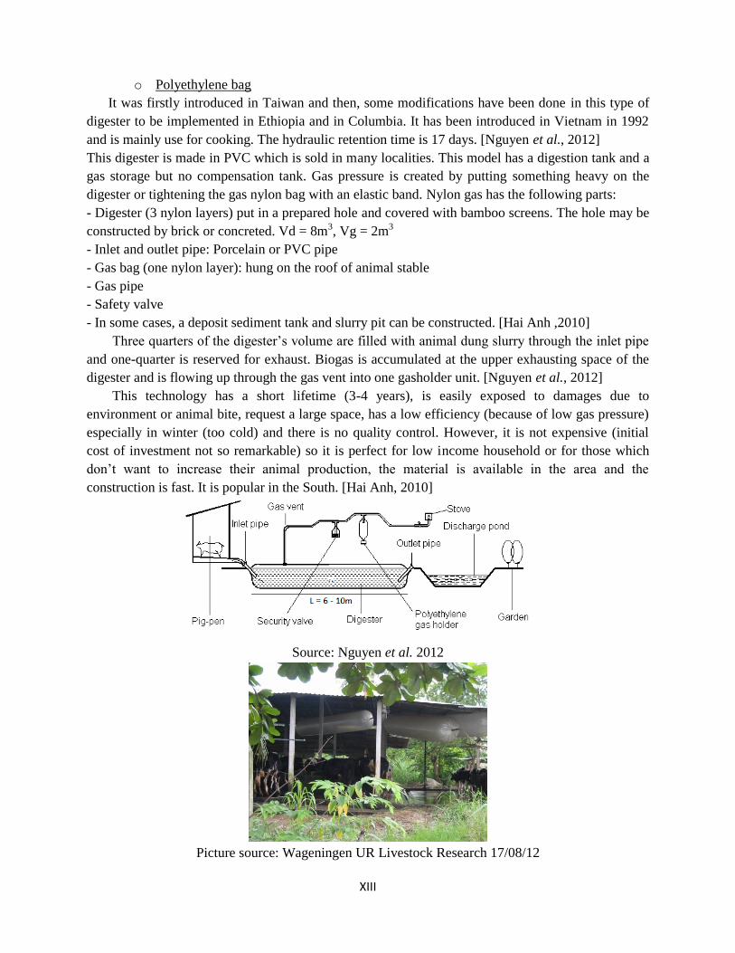
XIII
o Polyethylene bag
It was firstly introduced in Taiwan and then, some modifications have been done in this type of
digester to be implemented in Ethiopia and in Columbia. It has been introduced in Vietnam in 1992
and is mainly use for cooking. The hydraulic retention time is 17 days. [Nguyen et al., 2012]
This digester is made in PVC which is sold in many localities. This model has a digestion tank and a
gas storage but no compensation tank. Gas pressure is created by putting something heavy on the
digester or tightening the gas nylon bag with an elastic band. Nylon gas has the following parts:
- Digester (3 nylon layers) put in a prepared hole and covered with bamboo screens. The hole may be
constructed by brick or concreted. Vd = 8m3, Vg = 2m3
- Inlet and outlet pipe: Porcelain or PVC pipe
- Gas bag (one nylon layer): hung on the roof of animal stable
- Gas pipe
- Safety valve
- In some cases, a deposit sediment tank and slurry pit can be constructed. [Hai Anh ,2010]
Three quarters of the digester’s volume are filled with animal dung slurry through the inlet pipe
and one-quarter is reserved for exhaust. Biogas is accumulated at the upper exhausting space of the
digester and is flowing up through the gas vent into one gasholder unit. [Nguyen et al., 2012]
This technology has a short lifetime (3-4 years), is easily exposed to damages due to
environment or animal bite, request a large space, has a low efficiency (because of low gas pressure)
especially in winter (too cold) and there is no quality control. However, it is not expensive (initial
cost of investment not so remarkable) so it is perfect for low income household or for those which
don’t want to increase their animal production, the material is available in the area and the
construction is fast. It is popular in the South. [Hai Anh, 2010]
Source: Nguyen et al. 2012
Picture source: Wageningen UR Livestock Research 17/08/12

XIV
o Covered lagoon
This technology is a manure storage lagoon with a cover, which traps gas produced during the
manure decomposition. The lagoon is suitable for liquid manure with less than 3% solids and the
hydraulic retention times are from 30 days to 55 days. For this type of digester, an impermeable
floating cover covers all or part of the lagoon. A concrete footing along the edge of the lagoon holds
the cover in place with an airtight seal. The CH4 produced in the lagoon is collected under the cover.
A pipe extracts the gas for use. Covered lagoon digesters require large lagoon volumes and a warmer
climate. Covered lagoons have low capital costs for the digester volume itself, but these systems are
not suitable for locations in cooler climates or where a high water table exists. The membrane to
cover the lagoon is in HDPE (imported from Thailand or Taiwan). The disadvantages of such lagoon
are: it occupies a large surface area, sediments blocks 30-40% of the treatment volume after 5-6 years
of operation (need a cleaning of the lagoon, which never happens so the efficiency is reduced) [GFA
a, 2011].
o VACVINA
This model has been developed in Viet Nam in 1998. It is an innovative, low-maintenance and
easy to build model. The siting, similar as all brick and concrete fixed dome biogas plants, reduces
land requirements to a minimum (available space is a major problem for many households). On the
other hand, its hybrid nature (plastic bag biogas reservoir) helps keep the cost down, and avoids
design leakages of methane emissions in an open compensation chamber. Biogas is collected in a
separated plastic bag hanging in the stable or kitchen roof. The gas pressure increases by using a
rubber rob wrapped around the gas storage bag. Therefore gas burners used for this digester type are
the same as for each plastic bag digester. According to Huu Luu et al. (2011), 20% of the Vacvina
users have less than 5 pigs, 43% have between 6-10 pigs and 28% have between 11 and 20 pigs. 8%
of the fixed dome users have less than 5 pigs, 30% have 6-10 pigs and 42% have between 11 and 20
pigs. It appears that the domes (KT1/2) could request more animals than Vacvina to be as efficient.

XV
Appendix XII: Details about the digesters in the USA
The schema at the end of this appendix presents the choice of a digester type for some kind of
manure handlings.
o The plug flow digester
These digesters have a long and narrow heated tank, often built underground. They request a high
solid content (11-13%), so can be used especially in dairy farms. As they are heated, they stay at a
constant temperature all the year, and so can maintain a constant gas production. [USEPA a 2006].
They usually operate at mesophilic or thermophilic temperature and are working well with a scrape
manure management system. The retention time is 15-20 years. In theory, manure flows as a plug,
and move through the outlet when new manure is added. Then, it can be discharged over an outlet
weir, while maintaining a gas tight atmosphere. But in practice, a different process can occur: the
manure does not remain as a plug and some of the manure flow through the digester faster than
others and some parts stay in the digester. Then, the biogas produced is used to heat the digester. The
excess of biogas can be used for the engine generator. Heat can also be recovered from the engine
generator and used for space or water heating for example. The excess of biogas can also be used to
produce electricity, using an engine generator, to offset the cost of purchased electricity, propane,
natural gas or fuel oil27.
Source: USEPA AgSTAR: http://www.epa.gov/agstar/anaerobic/ad101/anaerobic-digesters.html
o The complete mix digester
These digesters have a mixing tank where manure accumulates before going into the digester.
Pumps and gravity are used to move the manure in the system. These digesters are also made up of a
vertical cylinder, and are made of steel or concrete with a gas-tight cover. As they are also heated,
they stay at a constant temperature all the year (can work at mesophilic or thermophilic temperature),
and so can maintain a consistent gas production. But they are more common in the warm climates,
where manure is flushed with water, which lower the solid content up to 3-10%. They can be used in
dairy and swine farms. [USEPA a 2006]. The gas is trapped with a gas-tight cover. Retention time is
10-20 days. The gas can then be used to heat the digester. The excess of gas can be used for the
engine generator. Heat can also be recovered from the engine generator and used for space or water
heating for example. The excess of biogas can also be used to produce electricity, using an engine
generator, to offset the cost of purchased electricity, propane, natural gas or fuel oil28.
27
Source : http://www.biogas.psu.edu/plugflow.html visited on the 25/08/12 28
Source : http://www.biogas.psu.edu/completemix.html visited on the 25/08/12
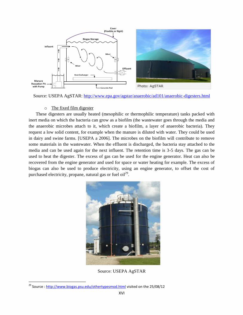
XVI
Source: USEPA AgSTAR: http://www.epa.gov/agstar/anaerobic/ad101/anaerobic-digesters.html
o The fixed film digester
These digesters are usually heated (mesophilic or thermophilic temperature) tanks packed with
inert media on which the bacteria can grow as a biofilm (the wastewater goes through the media and
the anaerobic microbes attach to it, which create a biofilm, a layer of anaerobic bacteria). They
request a low solid content, for example when the manure is diluted with water. They could be used
in dairy and swine farms. [USEPA a 2006]. The microbes on the biofilm will contribute to remove
some materials in the wastewater. When the effluent is discharged, the bacteria stay attached to the
media and can be used again for the next influent. The retention time is 3-5 days. The gas can be
used to heat the digester. The excess of gas can be used for the engine generator. Heat can also be
recovered from the engine generator and used for space or water heating for example. The excess of
biogas can also be used to produce electricity, using an engine generator, to offset the cost of
purchased electricity, propane, natural gas or fuel oil29.
Source: USEPA AgSTAR
29
Source : http://www.biogas.psu.edu/othertypesmod.html visited on the 25/08/12

XVII
o The covered lagoon
The methane is capture by the lagoon, which is covered by a flexible or floating gas tight cover.
The manure is stored and the gas is piped out to be flared or used on-farm. They request a low solid
content (less than 3%) and can be used for swine and dairy manure. They are not heated, so the
quantity of gas available varies over the year and less gas is produced when the temperature is low.
This is why the farms that have this digester and are located in the regions that have a high year
round temperature, can produce biogas for energy (heat recovery can be used to heat swine nursery
for example), reduce odors or increase the nutrient content of the effluent. These digesters are not
expensive and are considered to be a simple technology available in the developed and developing
countries (whereas the 3 technologies presented above are present in developed countries only).
[USEPA a 2006]. The retention time is quite long (30-45 days) and the dilution factor is high. They
are typically used with a flush manure management system. Sometimes, if they have enough biogas
produced, these digesters can use an engine generator. If they don’t (colder climate), then the biogas
is just flared for odor control and GHGs reduction30.
Sources: USEPA AgSTAR: http://www.epa.gov/agstar/anaerobic/ad101/anaerobic-digesters.html
Source: AgSTAR, no date
30
Source : http://www.biogas.psu.edu/coveredlagoon.html visited on the 25/08/12

XVIII
Appendix XIII: Consequences of the change of the capital cost (with
the inflation rate) in the USA (above) and Vietnam (below)

XIX
Appendix XIV: USEPA (2006) results for the USA and Vietnam
before tax
o USA MAC curves
o USA mitigation potential

XX
o Vietnam MAC curves
o Vietnam abatement potential

XXI
Appendix XV: Cost-benefit analysis for a covered lagoon in a 940
pig farm (Payback method)
Costs Benefits Payback period
Tank
Pumping and
mixing
Piping
Digester
Building
Other
5302
21865
84375
126706
267233
226054
Electricity sales
REC
5870
4696
With grants:
398651/8348 = 48 years
Without grants:
731535/8348 = 88 years
Total capital costs 731535
- Possible grants 332884
Net cost 398651 Yearly benefits 5870+4696-
2218= 8348 O&M 2218
Source: RCM international, 2012
This cost-benefit estimate has been done for a farm size far below the minimal number of animal
requested to run a digester in a profitable way according to AgSTAR in North Carolina, the first state
for pig production. This table summarizes the costs and potential benefits of such a project. In this
case, the farmer will finish paying his initial investment after 48 years if he had helps from USDA
and NCRS for building the digester (which is not always the case and the amount of the grants
changes from state to state). If he had not, the payment will be “refunded” only 88 years afterwards.
This project is too expensive for the little amount of benefits that the farmer could have. This is why
a minimum number of animals in the farms to produce a minimum amount of biogas could be
necessary.

XXII
Appendix XVI: Inventory and digesters distribution in the USA
o Dairy inventory and farm size

XXIII
o Swine inventory and farm size

XXIV
o Digester distribution
Source graphs: USDA NASS and AgSTAR

XXV
Appendix XVII: Climate zones in the USA and the digesters
distribution
The digesters in the dairy farms are within the purple outline and the ones in the pig farms are within
the yellow outline. The more the outline is thick, the more digesters are found in this place.
40th parallel

XXVI
Appendix XVIII: Methodology used for the geographic distribution
study
We said that, because the lagoon is unheated, it will request to be built in states where there is
low temperature variability, and a warm climate. Indeed, covered lagoons require large capacities to
treat the liquid manure properly at low temperatures (which is expensive and usually not cost-
effective). Therefore, covered lagoons for energy recovery (electricity and heat) are feasible only in
moderate to warm climates, where additional heat will not be required. Thus we consider that the
states above the 40th parallel could not build this kind of digester. So the lagoon could be applied to
50% of the territory. In the colder state, some lagoon could be built but only to solve odor problems.
As the aim of the study is to take into account the energy recovery, we will suppose that no lagoon
can be built in the states above the 40th parallel. Then, the lagoon is less efficient than the others
digesters, it will request more animals especially for the one that have an engine for electricity
production. The USA will be shared into 4 equal zones (North-West, North-East, South-West, and
South-East). The North-West part will go from Washington-Oregon to North-Dakota-Nebraska, the
South-West includes the states from California to Kansas-Texas, The South-East includes Missouri,
Kentucky, Virginia and the southern states, and the rest represents the North-East part. 47.2% of the
dairy cows are in the North-East of the USA, 33.6% are in the South West, 12.1% are in the North
West and 7.1% are in the South East, according to USDA NASS in 2010. Moreover, among 29 states
where the inventory could have been found in 2007 (no data after 2007), half of them have more than
500 cows and they are almost all located at the west part of the USA. Thus, we consider that the
lagoon with an engine applies to 25% of the territory (low temperature variation and big herd size in
the South West of the USA) and 33.6% of the dairy cows, and those without an engine apply to 7.1%
of the dairy cows (South East). For pigs, 61% of them are in the North East of the USA, 21.3% are in
the South East, 10.1% are in the South West and 7.5% are in the North West and almost all the states
where the inventory per herd size could have been found have more than 2000 pigs. Thus we
consider that lagoon in pig farm apply to 50% of the territory. The one with an engine can apply to
21.3% of the pigs in the South East and the one without can apply to 10.1% of the pigs in the South
West. For the heated digesters (plug flow, complete mix and fixed film) in dairy farms, they do not
have the problem of the temperature variation, and they are more efficient, so they could be applied
to the whole territory and all types of farms.
So, the information given above enables us to have a geographical distribution of the
technologies according bio-physical parameters, without any consideration of the economics.
However, we need to use the results of this study to be able to distinguish the heated digesters that
could be applied everywhere. Thus, we need to take into account the price of each technology among
the region where we could find many technologies to avoid double counting effects. For the pig
farms, the complete mix with an engine appeared to be cheaper than the plug flow and the North East
part has the highest amount of animals, so we will suppose the complete mix will be especially
applied in this part and will concern 61% of the pig population. Thus the plug flow with engine will
be supposed to be especially applied in the North-West part of the country and will concern 7.5% of
the animals (here we suppose the farmers can obtain the high solid content requested for this
technology while adding co-products). For dairy farms, most of the animals can be found in the
North-East part and the cheapest technologies are the plug flow and the complete mix with an engine

XXVII
(this also the part where most of the technologies in 2010 have been adopted). Thus, we will suppose
these 2 technologies will be the most applied in this part of the USA and will be adopted equally.
Thus, each one of these options will concern 23.6% of the dairy cows. And finally these options
without engine and the fixed film digester will be assumed to be the most applied in the North West
part of the USA and they will also share the same amount of animals. Thus, each one of them will
concern 4% of the animals.

XXVIII
Appendix XIX: Vietnamese regions and comparison of 3 regions
Source: Eastern Research Group (2010)
A comparison of 3 regions (Northern Mountain, North Central and South Central) in Vietnam
and 2 digesters has been done by Huu Luu et al. in 2011. In the mountain area, the animal husbandry
represents 30.2% of the activities, the mean temperature is 22.4°C, 1500 digesters can be found in
2008 (there are not a lot of pig farms in this area). In the North Central region (more than 1 million
pigs, with an average of 18 animals per households, 66% of the biogas users have between 10 and 20
pigs), 89.6% of the households are rural, the mean temperature is 23-24°C, 8000 digesters can be
found (especially domes), the humidity is 85-87%. Finally in the South Central region, we can found
even less pigs than in the mountain area, thus the number of digesters is also lower (800), especially
the dome digesters, the temperature is 26,7°C, and the humidity is 79%.

XXIX
Appendix XX: Picture of a failed lagoon
Source: Mattew Carr, Advisor Renewable Energy, SNV, 25/06/12

XXX
Appendix XXI: Comparison of the MAC curves under 2 implied
adoption rate assumptions in Vietnam
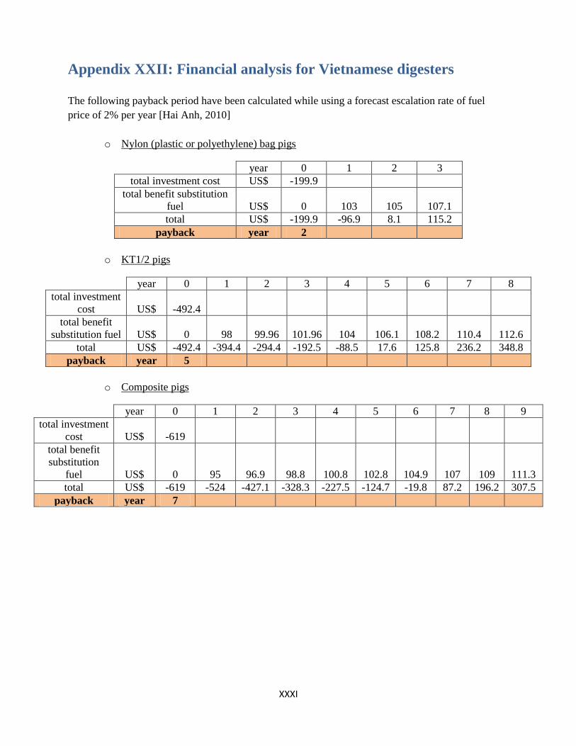
XXXI
Appendix XXII: Financial analysis for Vietnamese digesters
The following payback period have been calculated while using a forecast escalation rate of fuel
price of 2% per year [Hai Anh, 2010]
o Nylon (plastic or polyethylene) bag pigs
year 0 1 2 3
total investment cost US$ -199.9
total benefit substitution
fuel US$
0 103 105 107.1
total US$ -199.9 -96.9 8.1 115.2
payback year 2
o KT1/2 pigs
year 0 1 2 3 4 5 6 7 8
total investment
cost US$ -492.4
total benefit
substitution fuel US$ 0 98 99.96 101.96 104 106.1 108.2 110.4 112.6
total US$ -492.4 -394.4 -294.4 -192.5 -88.5 17.6 125.8 236.2 348.8
payback year 5
o Composite pigs
year 0 1 2 3 4 5 6 7 8 9
total investment
cost US$ -619
total benefit
substitution
fuel US$ 0 95 96.9 98.8 100.8 102.8 104.9 107 109 111.3
total US$ -619 -524 -427.1 -328.3 -227.5 -124.7 -19.8 87.2 196.2 307.5
payback year 7

XXXII
Appendix XXIII: Effect of the change in the discount rate in
Vietnam (10% above, 13% below)

XXXIII
Appendix XXIV: Methodology for the MAC curves building while
taking into account a progressive adoption rate (5 or 10%) and
extract of the break-even price calculation (10% rate)
For one digester type, we consider that the costs and revenues used in this study are
representative of a “mean” single farm. Then we take a sample of 100 farms (all the same), and we
suppose the full adoption of the technology the first year (everything is multiplied by 100). Here
again, the emission reduction without implied adoption rate is calculated to be used for the break-
even price formula. We can see that indeed, the break-even price, calculated with the same
methodology than before, is the same than with the single farm. Then, among these 100 farms, we
will suppose that only 10% the first year adopt the technology (and 20% the second year, 30% the
third, and so on, 100% from the 10th to the 20th year). So, the first year, the costs, revenue and
emission reduction found for the single farm will be multiplied by 10. The capital annuity (capital
cost/S, CA) is calculated because the S factor presented before applies only to the capital costs. All
the parameters are annualized. Then, for the following year until the 10th, the capital costs are always
the same because each year the same amounts of farms adopt the technology. The capital annuity is
thus, the total capital cost of these 10 extra farms divided by S plus the capital annuity of the past
year which is actually the same. So the capital annuity of the second year CA2 = CA1*2, the one for
the third year is CA1*3 and so on. The second year, the labor costs, revenue and emissions reduction
are the one for the single farm multiplied by the number of farms that adopt the technology, namely
20, and so on until the 10th year. The break-even price calculation is always the same and the amount
does not change over the time. The 10th year, we have the full adoption, then from the 11th to the 20th
year, the capital costs are inexistent, and the capital annuity, labor cost, revenue, and emission
reduction are always the same than the 10th year’s ones. The break-even price never changes. The
following tables present an example of the break-even price calculation with this methodology for
the plug flow digester in the USA with an adoption rate of 10% per year. Then only the abatement
potential will change over time and its incremental value is not the same if we consider the full
adoption the first year, or an adoption rate (10% or 5%).

XXXIV
Single representative farm
per t output
CC 423.3446
VC (labor) per yr 1.80
VC (labor) tot 36
Time period 20
Rev elect yr 91.08634
Tot rev 1821.727
ER per yr 0.605458
ER total 12.1
S 8.513564
Pnew -65.3
discount rate 10%
Capital annuity 49.7
ER per yr X axis 0.298188
ER per year X axis
(MMtCO2) 5.461476
year
1
year
2
year
3
year
4
year
5
year
6
year
7
year
8
year
9
year
10
year
11
CC 42 42 42 42 42 42 42 42 42 42 -
VC (labor)
per yr 0.18 0.36 0.54 0.72 0.90 1.08 1.26 1.44 1.62 1.80 1.80
Time
period 20 20 20 20 20 20 20 20 20 20 20
Rev elect
yr 9 18 27 36 46 55 64 73 82 91 91
ER per yr 0.06 0.12 0.18 0.24 0.30 0.36 0.42 0.48 0.54 0.61 0.61
ER total 1 2 4 5 6 7 8 10 11 12 12
S 8.51 8.51 8.51 8.51 8.51 8.51 8.51 8.51 8.51 8.51 8.51
Pnew
-
65.3
-
65.3
-
65.3
-
65.3
-
65.3
-
65.3
-
65.3
-
65.3
-
65.3
-
65.3
-
65.3
No. farms
adopt: 10% 20% 30% 40% 50% 60% 70% 80% 90% 100% 100%
Capital
annuity 5 10 15 20 25 30 35 40 45 50 50
ER per yr
X axis 0.03 0.06 0.09 0.12 0.15 0.18 0.21 0.24 0.27 0.30 0.30
ER per
year X axis
(MMtCO2) 0.55 1.09 1.64 2.18 2.73 3.28 3.82 4.37 4.92 5.46 5.46

XXXV
Appendix XXV: AgSTAR assumption test (500 cows, 2000 pigs)
o Pigs
number of animals 0 940 2000 1793 2504
power produced (kWh/yr) 0 117404 249795
power produced per head
(kWh/yr) 0 124.8979 124.8975 124.8975 124.8975
total cost ($) 0 731535 738614
cost per head ($/head) 0 778.2287 369.307 448.982 174.8565
grants USDA ($) 0 182883.8 184653.5
grants USDA per head
($/head) 0 194.5572 92.32675 112.2455 0
grants NRCS ($) 0 152167.2 323760
grants NRCS per head
($/head) 0 161.88 161.88 161.88 0
net cost ($) 0 396484.1 230200.5
net cost per head ($/head) 0 421.7915 115.1003 174.8565 174.8565
electricity sales ($/yr) 0 5870.2 12489.75
electricity sales per head ($/yr) 0 6.244894 6.244875 6.244875 6.244875
Renewable Energy Credit
($/yr) 0 4696.16 9991.8
REC per head ($/yr/head) 0 4.995915 4.9959 4.9959 4.9959
O&M costs ($/yr) 0 2348.08 4995.9
O&M costs per head
($/yr/head) 0 2.497957 2.49795 2.49795 2.49795
yearly benefits ($/yr) 0 8218.28 17485.65
yearly benefits per head
($/yr/head) 0 8.742851 8.742825 8.742825 8.742825
payback with grants 0 48.24416 13.16511 20
payback without grants 0 89.01315 42.24115
20
Explanation of the calculations for a 20 years payback with grants:
The yearly benefits per head do not change, thus it is possible to know the value of the net cost for a
payback of 20 years.
Here again, the grants NRCS per head do not change (it is always $760 for 1000 lbs of animal), so it
is possible to know the value of the total costs per head for a 20 years payback.
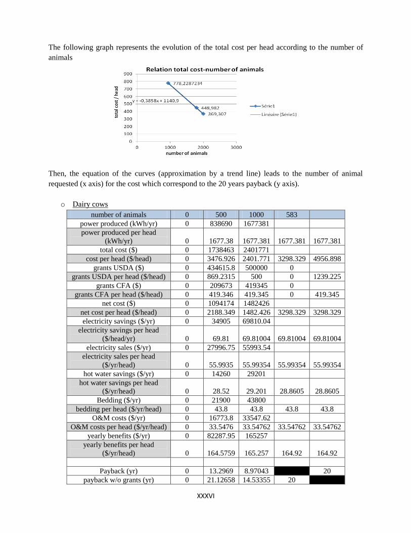
XXXVI
The following graph represents the evolution of the total cost per head according to the number of
animals
Then, the equation of the curves (approximation by a trend line) leads to the number of animal
requested (x axis) for the cost which correspond to the 20 years payback (y axis).
o Dairy cows
number of animals 0 500 1000 583
power produced (kWh/yr) 0 838690 1677381
power produced per head
(kWh/yr) 0 1677.38 1677.381 1677.381 1677.381
total cost ($) 0 1738463 2401771
cost per head ($/head) 0 3476.926 2401.771 3298.329 4956.898
grants USDA ($) 0 434615.8 500000 0
grants USDA per head ($/head) 0 869.2315 500 0 1239.225
grants CFA ($) 0 209673 419345 0
grants CFA per head ($/head) 0 419.346 419.345 0 419.345
net cost ($) 0 1094174 1482426
net cost per head ($/head) 0 2188.349 1482.426 3298.329 3298.329
electricity savings ($/yr) 0 34905 69810.04
electricity savings per head
($/head/yr) 0 69.81 69.81004 69.81004 69.81004
electricity sales ($/yr) 0 27996.75 55993.54
electricity sales per head
($/yr/head) 0 55.9935 55.99354 55.99354 55.99354
hot water savings ($/yr) 0 14260 29201
hot water savings per head
($/yr/head) 0 28.52 29.201 28.8605 28.8605
Bedding ($/yr) 0 21900 43800
bedding per head ($/yr/head) 0 43.8 43.8 43.8 43.8
O&M costs ($/yr) 0 16773.8 33547.62
O&M costs per head ($/yr/head) 0 33.5476 33.54762 33.54762 33.54762
yearly benefits ($/yr) 0 82287.95 165257
yearly benefits per head
($/yr/head) 0 164.5759 165.257 164.92 164.92
Payback (yr) 0 13.2969 8.97043
20
payback w/o grants (yr) 0 21.12658 14.53355 20

XXXVII
Here we supposed that the yearly benefits per head do not change to simplify the calculations (a
mean has been done between the yearly benefits for 500 and 1000 cows). Moreover, it appears that in
both case, 55.49% of the power produced correspond to savings (so that is the amount of power the
farm needs) and that the rest (44.51%) is sold.
The same methodology for dairy has been used to calculate the amount of animals requested to have
a 20 years payback without grants. With grants, the quantity found is negative, which mean that there
is no minimum number; every kind of dairy farm could be profitable if there are these grants.