cosmin ilut hikaru saijo - canon-igs.org · learning, con dence, and business cycles cosmin ilut...
TRANSCRIPT
Learning, Confidence, and Business Cycles
Cosmin Ilut Hikaru Saijo
Duke & NBER UC Santa Cruz
CIGS Conference on Macroeconomic Theory and PolicyMay 2016
Ilut, Saijo Learning, Confidence, and Business Cycles 1 / 27

Parsimonious mechanism for business cycle dynamics
Propose: Endogenous idiosyncratic uncertaintyI firms learn about own profitability prospects
Behaves as if linear RBC model with endogenously determined
1 Countercyclical labor wedge and spreads (from excess returns)
2 Co-movement from demand shocks
3 Amplification, propagation and hump-shaped dynamics
Ilut, Saijo Learning, Confidence, and Business Cycles 2 / 27
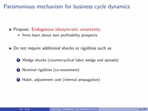
Parsimonious mechanism for business cycle dynamics
Propose: Endogenous idiosyncratic uncertaintyI firms learn about own profitability prospects
Do not require additional shocks or rigidities such as
1 Wedge shocks (countercyclical labor wedge and spreads)
2 Nominal rigidities (co-movement)
3 Habit, adjustment cost (internal propagation)
Ilut, Saijo Learning, Confidence, and Business Cycles 3 / 27
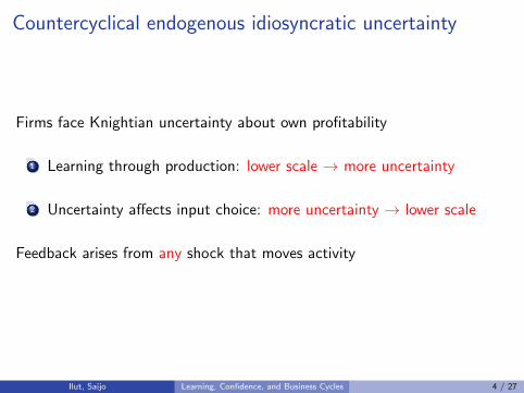
Countercyclical endogenous idiosyncratic uncertainty
Firms face Knightian uncertainty about own profitability
1 Learning through production: lower scale → more uncertainty
2 Uncertainty affects input choice: more uncertainty → lower scale
Feedback arises from any shock that moves activity
Ilut, Saijo Learning, Confidence, and Business Cycles 4 / 27

Countercyclical idiosyncratic uncertainty shows up
As countercyclical wedges: labor and asset prices move ’too much’compared to what econometrician measures
I rationalize ’excess volatility’
In linear decision rules at firm level
In the cross-sectional average through aggregation
Ilut, Saijo Learning, Confidence, and Business Cycles 5 / 27

Model: Preferences
Representative household: recursive multiple priors utility
Ut(C ; st) = lnCt − ϕH1+ηt
1 + η+ β min
p∈Pt(st)Ep[Ut+1(C ; st , st+1)]
Pt(st): one-stead-ahead set of probability distributions
Larger set Pt(st) → less confidence
Ilut, Saijo Learning, Confidence, and Business Cycles 6 / 27

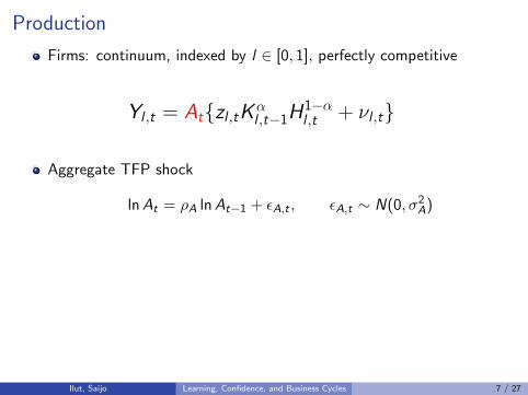
Production
Firms: continuum, indexed by l ∈ [0, 1], perfectly competitive
Yl ,t = At{zl ,tKαl ,t−1H
1−αl ,t + νl ,t}
Aggregate TFP shock
lnAt = ρA lnAt−1 + εA,t , εA,t ∼ N(0, σ2A)
Idiosyncratic TFP shock
zl ,t = (1− ρz)z + ρzzl ,t−1 + εz,l ,t , εz,l ,t ∼ N(0, σ2z )
Idiosyncratic additive shock, νl ,t ∼ N(0, σ2ν)
Ilut, Saijo Learning, Confidence, and Business Cycles 7 / 27
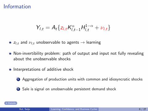
Information
Yl ,t = At{zl ,tKαl ,t−1H
1−αl ,t + νl ,t}
zl ,t and νl ,t unobservable to agents → learning
Non-invertibility problem: path of output and input not fully revealingabout the unobservable shocks
Interpretations of additive shock
1 Aggregation of production units with common and idiosyncratic shocks
2 Sale is signal on unobservable persistent demand shock
Details
Ilut, Saijo Learning, Confidence, and Business Cycles 8 / 27

Heterogeneous-firm RBC model
Firms: choose {Kl ,t ,Hl ,t , Il ,t} to maximize
E ∗0
∞∑t=0
Mt0Dl ,t
I M t0 : prices of contingent claims, under worst case probabilities
Dl,t = Yl,t −WtHl,t − Il,t
Resource constraint:
Yt = Ct + It + Gt
lnGt = (1− ρg )G + ρg lnGt−1 + εg ,t , εg ,t ∼ N(0, σ2g )
Ilut, Saijo Learning, Confidence, and Business Cycles 9 / 27

Timeline of events within a period
Aggregate shocks(observable)
Given forecasts and variance ofhidden TFP, choose inputs,labor market clearing
Stage 1 Stage 2
Idiosyncratic shocks(unobservable)
Production, updateforecasts and variance ofhidden TFP
Investment,consumption,asset purchase
RCE
Ilut, Saijo Learning, Confidence, and Business Cycles 10 / 27

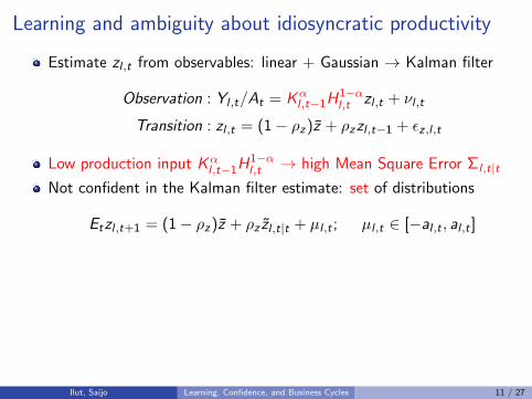
Learning and ambiguity about idiosyncratic productivity
Estimate zl ,t from observables: linear + Gaussian → Kalman filter
Observation : Yl ,t/At = Kαl ,t−1H
1−αl ,t zl ,t + νl ,t
Transition : zl ,t = (1− ρz)z + ρzzl ,t−1 + εz,l ,t
Low production input Kαl ,t−1H
1−αl ,t → high Mean Square Error Σl ,t|t
Not confident in the Kalman filter estimate: set of distributions
Etzl ,t+1 = (1− ρz)z + ρz zl ,t|t + µl ,t ; µl ,t ∈ [−al ,t , al ,t ]
Confidence lower when estimation uncertainty is higher
−al ,t = −ηa√
Σl ,t|t
I Distributions “close” to filter estimate (relative entropy distance)
Ilut, Saijo Learning, Confidence, and Business Cycles 11 / 27
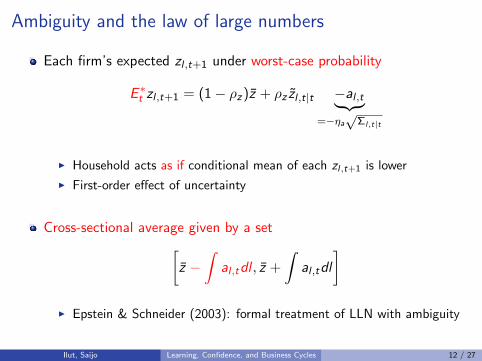
Ambiguity and the law of large numbers
Each firm’s expected zl ,t+1 under worst-case probability
E ∗t zl ,t+1 = (1− ρz)z + ρz zl ,t|t −al ,t︸ ︷︷ ︸=−ηa√
Σl,t|t
I Household acts as if conditional mean of each zl,t+1 is lower
I First-order effect of uncertainty
Cross-sectional average given by a set[z −
∫al ,tdl , z +
∫al ,tdl
]I Epstein & Schneider (2003): formal treatment of LLN with ambiguity
Ilut, Saijo Learning, Confidence, and Business Cycles 12 / 27

Linearized solution
1 Filtering problem is linear → analytic law of motion for Σl ,t|t
I Inputs have first-order effect on the level of posterior variance
2 First-order feedback from uncertainty to decision rules through −al ,t
3 In turn, linear decision rules → easy aggregation
I Cross-sectional mean: sufficient statistic for tracking distributions
Ilut, Saijo Learning, Confidence, and Business Cycles 13 / 27
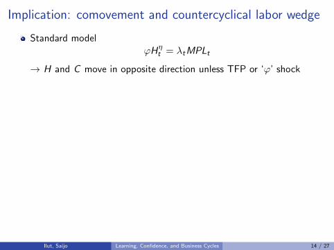
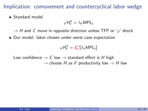
Implication: comovement and countercyclical labor wedge
Standard modelϕHη
t = λtMPLt
→ H and C move in opposite direction unless TFP or ‘ϕ’ shock
Our model: labor chosen under worst case expectation
ϕHηt = E ∗t [λtMPLt ]
Low confidence → C low → standard effect is H high→ choose H as if productivity low → H low
Labor wedge: implicitly define labor tax
ϕHηt = (1− τt)λtMPLt ⇒ E ∗t [λtMPLt ]
λtMPLt= 1− τt
Low confidence → econometrician rationalizes ‘surprisingly low’ H byhigh labor tax
Ilut, Saijo Learning, Confidence, and Business Cycles 14 / 27

Implication: countercyclical ex-post excess return
Euler conditions for capital and risk-free assets
λt = βE ∗t [λt+1RKt+1]
λt = βE ∗t [λt+1Rt ]
→ under linearization, E ∗t RKt+1 − Rt = 0
Pricing based on worst case 6= econometrician’s DGP
During low confidence times, demand for capital ‘surprisingly low’→ ex-post excess return RK
t+1 − Rt high
Implication extends to defaultable corporate bonds→ countercyclical excess bond premia (Gilchrist & Zakrajsek 2012)
Ilut, Saijo Learning, Confidence, and Business Cycles 15 / 27
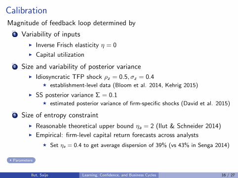
CalibrationMagnitude of feedback loop determined by
1 Variability of inputs
I Inverse Frisch elasticity η = 0
I Capital utilization
2 Size and variability of posterior varianceI Idiosyncratic TFP shock ρz = 0.5, σz = 0.4
F establishment-level data (Bloom et al. 2014, Kehrig 2015)
I SS posterior variance Σ = 0.1F estimated posterior variance of firm-specific shocks (David et al. 2015)
3 Size of entropy constraint
I Reasonable theoretical upper bound ηa = 2 (Ilut & Schneider 2014)I Empirical: firm-level capital return forecasts across analysts
F Set ηa = 0.4 to get average dispersion of 39% (vs 43% in Senga 2014)
Parameters
Ilut, Saijo Learning, Confidence, and Business Cycles 16 / 27

IRF to aggregate TFP shock
5 10 15 200
1
2
Output
Per
cent
dev
iatio
n
5 10 15 20
0
2
4
6
8Investment
5 10 15 200.08
0.1
0.12
0.14
0.16
Consumption
5 10 15 20
0
1
2
Hours
5 10 15 20−0.08
−0.06
−0.04
−0.02
0
Labor wedge
5 10 15 20−1
−0.5
0
Ex−post excess return
5 10 15 20
0
0.02
0.04
0.06
Cross−sectional mean of worst−case TFP
5 10 15 20−1
0
1Cross−sectional mean of realized TFP
BaselinePassiveRE
Figure 1: Impulse response to an aggregate TFP shock. Thick black solid line is our baselinemodel with active learning, thin blue dashed line is the model with passive learning, andthick red dashed line is the frictionless RBC model.
51
Ilut, Saijo Learning, Confidence, and Business Cycles 17 / 27

IRF to aggregate TFP shock
5 10 15 200
1
2
Output
Per
cent
dev
iatio
n
5 10 15 20
0
2
4
6
8Investment
5 10 15 200.08
0.1
0.12
0.14
0.16
Consumption
5 10 15 20
0
1
2
Hours
5 10 15 20−0.08
−0.06
−0.04
−0.02
0
Labor wedge
5 10 15 20−1
−0.5
0
Ex−post excess return
5 10 15 20
0
0.02
0.04
0.06
Cross−sectional mean of worst−case TFP
5 10 15 20−1
0
1Cross−sectional mean of realized TFP
BaselinePassiveRE
Figure 1: Impulse response to an aggregate TFP shock. Thick black solid line is our baselinemodel with active learning, thin blue dashed line is the model with passive learning, andthick red dashed line is the frictionless RBC model.
51
Ilut, Saijo Learning, Confidence, and Business Cycles 18 / 27

IRF to government spending shock
5 10 15 20
0.2
0.4
0.6
Output
Per
cent
dev
iatio
n
5 10 15 20
0
0.5
1
1.5
Investment
5 10 15 20
−0.01
0
0.01
Consumption
5 10 15 20
0.2
0.4
0.6
Hours
5 10 15 20
−0.02
−0.01
0Labor wedge
5 10 15 20−0.3
−0.2
−0.1
Ex−post excess return
5 10 15 200
0.01
0.02
Cross−sectional mean of worst−case TFP
5 10 15 20−1
0
1Cross−sectional mean of realized TFP
BaselinePassiveRE
Figure 2: Impulse response to a government spending shock. Thick black solid line is ourbaseline model with active learning, thin blue dashed line is the model with passive learning,and thick red dashed line is the frictionless RBC model.
52
Ilut, Saijo Learning, Confidence, and Business Cycles 19 / 27

IRF to government spending shock
5 10 15 20
0.2
0.4
0.6
Output
Per
cent
dev
iatio
n
5 10 15 20
0
0.5
1
1.5
Investment
5 10 15 20
−0.01
0
0.01
Consumption
5 10 15 20
0.2
0.4
0.6
Hours
5 10 15 20
−0.02
−0.01
0Labor wedge
5 10 15 20−0.3
−0.2
−0.1
Ex−post excess return
5 10 15 200
0.01
0.02
Cross−sectional mean of worst−case TFP
5 10 15 20−1
0
1Cross−sectional mean of realized TFP
BaselinePassiveRE
Figure 2: Impulse response to a government spending shock. Thick black solid line is ourbaseline model with active learning, thin blue dashed line is the model with passive learning,and thick red dashed line is the frictionless RBC model.
52
Ilut, Saijo Learning, Confidence, and Business Cycles 20 / 27
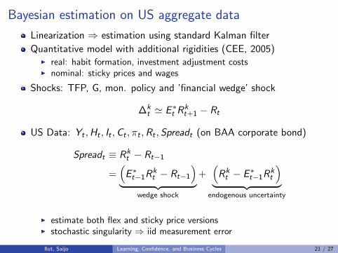
Bayesian estimation on US aggregate data
Linearization ⇒ estimation using standard Kalman filter
Quantitative model with additional rigidities (CEE, 2005)I real: habit formation, investment adjustment costsI nominal: sticky prices and wages
Shocks: TFP, G, mon. policy and ’financial wedge’ shock
∆kt ' E ∗t R
kt+1 − Rt
US Data: Yt ,Ht , It ,Ct , πt ,Rt ,Spreadt (on BAA corporate bond)
Spreadt ≡ Rkt − Rt−1
=(E ∗t−1R
kt − Rt−1
)︸ ︷︷ ︸
wedge shock
+(Rkt − E ∗t−1R
kt
)︸ ︷︷ ︸
endogenous uncertainty
I estimate both flex and sticky price versionsI stochastic singularity ⇒ iid measurement error
Ilut, Saijo Learning, Confidence, and Business Cycles 21 / 27
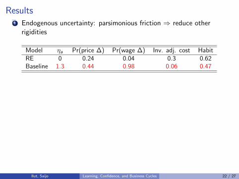
Results1 Endogenous uncertainty: parsimonious friction ⇒ reduce other
rigidities
Model ηa Pr(price ∆) Pr(wage ∆) Inv. adj. cost HabitRE 0 0.24 0.04 0.3 0.62Baseline 1.3 0.44 0.98 0.06 0.47
2 Endogenous uncertainty model fits data betterI marginal data density is higher (both flex and sticky price versions)I under RE: observed spread is mostly just measurement errorI but well fitted under model with endogenous uncertainty
3 Variance decomposition: financial shock more important with learning
Model (sticky price) Y H I C π R
RE 0.15 0.23 0.12 0.22 0.88 0.90Baseline 0.73 0.81 0.76 0.61 0.88 0.84
Ilut, Saijo Learning, Confidence, and Business Cycles 22 / 27
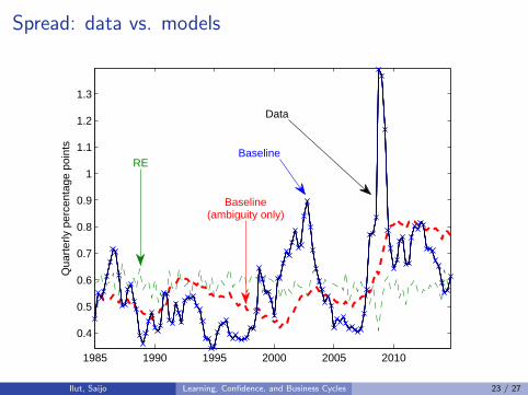
Spread: data vs. models
1985 1990 1995 2000 2005 2010
0.4
0.5
0.6
0.7
0.8
0.9
1
1.1
1.2
1.3
Qua
rter
ly p
erce
ntag
e po
ints
RE
Baseline(ambiguity only)
Baseline
Data
Ilut, Saijo Learning, Confidence, and Business Cycles 23 / 27

Endogenous uncertainty: countercyclical spread ⇒ bus.cycle comovement
5 10 15 20−2
−1.5
−1
−0.5
Output
Per
cent
dev
iatio
n
5 10 15 20
−6
−4
−2
Investment
5 10 15 20
−1
−0.8
−0.6
−0.4
−0.2
0
Consumption
5 10 15 20
−1
−0.8
−0.6
−0.4
−0.2
Hours
BaselineRE counterfactual
Ilut, Saijo Learning, Confidence, and Business Cycles 24 / 27

Results1 Endogenous uncertainty: parsimonious friction ⇒ reduce other
rigidities
Model ηa Pr(price ∆) Pr(wage ∆) Inv. adj. cost HabitRE 0 0.24 0.04 0.3 0.62Baseline 1.3 0.44 0.98 0.06 0.47
2 Endogenous uncertainty model fits data betterI marginal data density is higher (both flex and sticky price versions)I under RE: observed spread is mostly just measurement errorI but well fitted under model with endogenous uncertainty
3 Variance decomposition: financial shock more important with learning
Model (sticky price) Y H I C π R
RE 0.15 0.23 0.12 0.22 0.88 0.90Baseline 0.73 0.81 0.76 0.61 0.88 0.84
Ilut, Saijo Learning, Confidence, and Business Cycles 25 / 27

Policy implication of endogenous uncertainty
Endogenous uncertainty ⇒ Policy matters
Policy experiment:
I modify Taylor rule to include adjustment to credit spread φspread
I lower output growth variation: from stabilizing endogenous uncertainty
Std. of output growthφspread Baseline Fixed uncertainty
0 0.60 0.60-0.5 0.59 0.60-1.0 0.57 0.60-1.5 0.52 0.63
Ilut, Saijo Learning, Confidence, and Business Cycles 26 / 27

Conclusion
Heterogeneous-firm business cycle model where firms face Knightianuncertainty about their own profitability
Feedback loop between uncertainty and economic activity produces
I Countercyclical labor wedge and ex-post excess return on capital
I Co-movement in response to non-TFP shocks
I Strong internal propagation with amplified and hump-shaped dynamics
Estimation: inference on rigidities and shocks
Policy implications
Ilut, Saijo Learning, Confidence, and Business Cycles 27 / 27

Interpreting the additive shock (νl ,t)
1 At the aggregate level, observationally equivalent to model wherefirms face unobservable demand shock
I Each unit of good l : provides sum of good specific and idiosyncraticquality
Yl,t =
Yl,t∑j=1
(zl,t + νl,j,t)
I where units produced Yl,t = Kαl,t−1H
1−αl,t
I Noisy signal about persistent quality zl,t : procyclical precision
Yl,t/Yl,t = zl,t + νl,t , νl,t ∼ N
(0,σ2ν
Yl,t
)I demand is a function of estimate of quality zl,t
2 Aggregation of production units with common and idio shocks
Return
Ilut, Saijo Learning, Confidence, and Business Cycles 1 / 16

Kalman filter
Estimate
zl ,t|t = zl ,t|t−1 + Gainl ,t(Yl ,t/At − zl ,t|t−1Fl ,t)
Kalman gain
Gainl ,t =
[F 2l ,tΣl ,t|t−1
F 2l ,tΣl ,t|t−1 + σ2
ν,t
]F−1l ,t
Mean square error
Σl ,t|t = (1− Gainl ,tFl ,t)Σl ,t|t−1
=σ2ν,tΣl ,t|t−1
F 2l ,tΣl ,t|t−1 + σ2
ν,t
Return
Ilut, Saijo Learning, Confidence, and Business Cycles 2 / 16

Illustration: distinguishing distributions
Return
Ilut, Saijo Learning, Confidence, and Business Cycles 3 / 16

Relative entropy distance
Agents consider the conditional means µ∗l ,t+1 that are sufficiently close tothe long run average of zero in the sense of relative entropy:
(µ∗l ,t+1)2
2ρ2zΣl ,t|t
≤ 1
2η2a
LHS: relative entropy between two normal distributions that share thesame variance ρ2
zΣl ,t|t but have different means (µ∗l ,t+1 and zero)
Return
Ilut, Saijo Learning, Confidence, and Business Cycles 4 / 16

Linearized solution
1 Filtering problem is linear → analytic law of motion for Σl ,t|tI Inputs have first-order effect on the level of posterior variance
Σl ,t−1|t−1 = εΣ,ΣΣl ,t−2|t−2 − εΣ,F Fl ,t−1, (1)
2 First-order feedback from uncertainty to decision rules through −al ,t
E ∗t zl ,t = εz,z ˆzl ,t−1|t−1 − εz,ΣΣl ,t−1|t−1, (2)
3 In turn, linear decision rules → easy aggregationI Cross-sectional mean: sufficient statistic for tracking distributions
E ∗t zt = εz,z ˆzt−1|t−1︸ ︷︷ ︸=0
−εz,ΣεΣ,ΣΣt−2|t−2 + εz,ΣεΣ,F Ft−1 (3)
where xt ≡∫xl ,tdl
Return
Ilut, Saijo Learning, Confidence, and Business Cycles 5 / 16
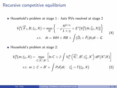
Recursive competitive equilibrium
Household’s problem at stage 1 : hats RVs resolved at stage 2
V h1 (−→θ l ,B; ξ1,X ) = max
H
{− ϕH
1+η
1 + η+ E ∗[V h
2 (m; ξ2,X )]
}s.t. m = WH + RB +
∫(Dl + Pl)θldl − G
(4)
Household’s problem at stage 2:
V h2 (m; ξ2,X ) = max
C ,−→θl ′,B′
[lnC + β
∫V h
1
(−→θl′,B ′; ξ′1,X
′)dF (X ′|X )
]s.t. m ≥ C + B ′ +
∫Plθ′ldl ; ξ′1 = Γ(ξ2,X ) (5)
Ilut, Saijo Learning, Confidence, and Business Cycles 6 / 16
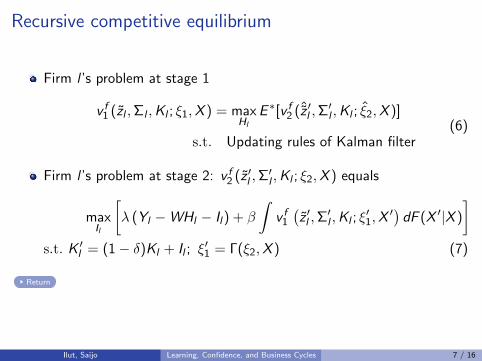
Recursive competitive equilibrium
Firm l ’s problem at stage 1
v f1 (zl ,Σl ,Kl ; ξ1,X ) = maxHl
E ∗[v f2 (ˆz ′l ,Σ′l ,Kl ; ξ2,X )]
s.t. Updating rules of Kalman filter(6)
Firm l ’s problem at stage 2: v f2 (z ′l ,Σ′l ,Kl ; ξ2,X ) equals
maxIl
[λ (Yl −WHl − Il) + β
∫v f1(z ′l ,Σ
′l ,Kl ; ξ
′1,X
′) dF (X ′|X )
]s.t. K ′l = (1− δ)Kl + Il ; ξ
′1 = Γ(ξ2,X ) (7)
Return
Ilut, Saijo Learning, Confidence, and Business Cycles 7 / 16
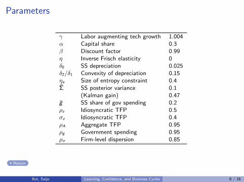
Parameters
γ Labor augmenting tech growth 1.004α Capital share 0.3β Discount factor 0.99η Inverse Frisch elasticity 0δ0 SS depreciation 0.025δ2/δ1 Convexity of depreciation 0.15ηa Size of entropy constraint 0.4Σ SS posterior variance 0.1
(Kalman gain) 0.47g SS share of gov spending 0.2ρz Idiosyncratic TFP 0.5σz Idiosyncratic TFP 0.4ρA Aggregate TFP 0.95ρg Government spending 0.95ρσ Firm-level dispersion 0.85
Return
Ilut, Saijo Learning, Confidence, and Business Cycles 8 / 16

HP-filtered moments (TFP shock only)
Data Our model RE
σ(y) 1.11 1.11 0.49σ(c)/σ(y) 0.72 0.11 0.17σ(i)/σ(y) 3.57 2.95 3.23σ(h)/σ(y) 1.64 1.02 0.86
σ(c, y) 0.86 0.72 0.85σ(i , y) 0.92 0.99 0.99σ(h, y) 0.88 0.99 0.99
σ(y , τl) -0.83 -0.95 0σ(h, τl) -0.97 -0.95 0
σ(yt , yt−1) 0.89 0.87 0.66σ(ht , ht−1) 0.95 0.88 0.66
σ(∆yt ,∆yt−1) 0.39 0.44 -0.06σ(∆ht ,∆ht−1) 0.71 0.52 -0.06
Note: We choose the st. dev of aggregate TFP shock so that the output st. dev in themodel matches the data.
Return
Ilut, Saijo Learning, Confidence, and Business Cycles 9 / 16
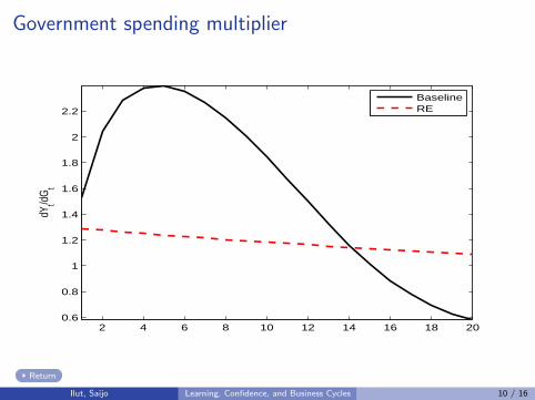
Government spending multiplier
2 4 6 8 10 12 14 16 18 200.6
0.8
1
1.2
1.4
1.6
1.8
2
2.2
dYt/d
Gt
BaselineRE
Return
Ilut, Saijo Learning, Confidence, and Business Cycles 10 / 16
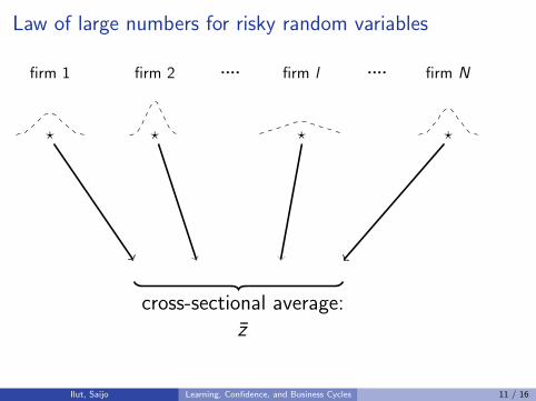
Law of large numbers for risky random variables
firm 1 firm 2 firm l firm N.... ....
? ? ? ?
cross-sectional average:z
Ilut, Saijo Learning, Confidence, and Business Cycles 11 / 16

Law of large numbers for ambiguous random variables
firm 1 firm 2 firm l firm N.... ....
2ηaρz√
Σl
cross-sectional average:???
Ilut, Saijo Learning, Confidence, and Business Cycles 12 / 16

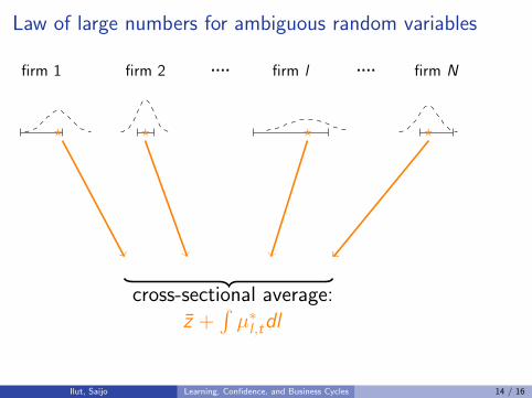
Law of large numbers for ambiguous random variables
firm 1 firm 2 firm l firm N.... ....
? ? ? ?
cross-sectional average:z +
∫µ∗l ,tdl
Ilut, Saijo Learning, Confidence, and Business Cycles 13 / 16
Law of large numbers for ambiguous random variables
firm 1 firm 2 firm l firm N.... ....
? ? ? ?
cross-sectional average:z +
∫µ∗l ,tdl
Ilut, Saijo Learning, Confidence, and Business Cycles 14 / 16

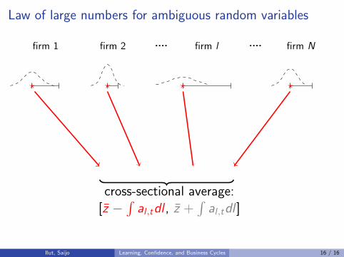
Law of large numbers for ambiguous random variables
firm 1 firm 2 firm l firm N.... ....
? ? ? ?
cross-sectional average:[z −
∫al ,tdl , z +
∫al ,tdl ]
Ilut, Saijo Learning, Confidence, and Business Cycles 15 / 16
Law of large numbers for ambiguous random variables
firm 1 firm 2 firm l firm N.... ....
? ? ? ?
cross-sectional average:[z −
∫al ,tdl , z +
∫al ,tdl ]
Ilut, Saijo Learning, Confidence, and Business Cycles 16 / 16