Corso di Relatività Generale

I ParteFondamenti di Geometria Differenziale e Relatività

Generale

Summary of Riemanian Geometry and Vielbein formulation

Manifolds

Introduction to manifolds

Privileged observers and affine manifolds

Both Newtonian Physics and Special Relativityhave privileged observers

Affine Manifold

Affine Manifolds

Curved Manifolds and Atlases

The intuitive idea of an atlas of open charts, suitably reformulated in mathematical terms,provides the very definition of a differentiable manifold

Homeomorphisms

Topology invariant underhomeomorphisms

Homeomorphic spaces

Open charts

Picture of an open chart

HomeomorphismHomeomorphism

Differentiable structure

M1

The axiom M2

Transitionfunctions

Picture of transition functions

The axiom M3

Differentiable Manifolds

This is a constructive definition

Smooth manifolds

Complex Manifolds

Example the SN sphere

The stereographic projection

The transition function

There are just two open charts and the transition function is the following one

Calculus on Manifolds

Functions on Manifolds

Local description

Gluing Rules

Global Functions

Germs of Smooth Functions

Germs atp2 M

Towards tangent spaces: Curves on a Manifold

Curves

Loops

Tangent vectors at a point p 2 M

Intuitively the tangent in p at a curve that starts from p is the curve’s initial direction

Tangent spaces at p 2 M

Example: tangent space at p 2 S2

Let us make this intuitive notion mathematically precise

Tangent vectors and germs

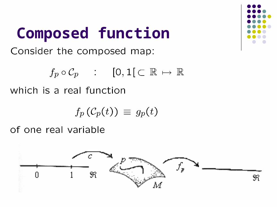
Composed function

Derivative = tangent vector

Differential operator

Tangent vectors and derivations of algebras

Algebra of germs

Derivations of algebras

Vector space of derivations

Vectors as differential operators

Vector controvariance

We haveWe have

wherewhere

Controvariant versus covariant vectors

Introducing differential forms

DEFINITION:

Cotangent space

DefinitionDefinition

Differential 1-forms at p 2 M

= dx

Why named differential forms

Covariance

Fibre bundles

Fibre Bundles

Definition: A Fibre--bundle E M F G, , , , is a geometrical

structure that consists of the following list of elements: 1. A differentiable manifold E named the total space

2. A differentialble manifold M named the base space

3. A differentiable manifold F named the standard fibre

4. A Lie group G named the structure group which acts as a transformation group on the standard fibre:

g G ; g : F F i e f F g f F. . ,

5. A surjection map :E M named the projection . If n=dim M and m=dim F, then we have dim E = n+m and p E , Fp= 1 p is an

m-dimensional manifold diffeomorphic to the standard fibre F . The manifold Fp is named the fibre at point p

6. A covering of the base space UA = M realized by a collection

U M of open subsets equipped with a diffeomorphism:

:U F U 1

such that p U f F , : p f p,

The map is named a local trivialization of the bundle

7 If we write p f fp, ( ), the map , :p pF F is the

diffeomorphism required by point 5) of the present definition. For all points p U U in the intersection of two local trivialization

domains, the composite map t p F Fp p , , :1 is an

element of the structure group: t p G named the transition

function. Furthermore, the transition function realizes a smooth map: t : U U G ; p f p t p f, ,

Il concetto di Spazio Fibrato

M denota lo spazio di base P denota lo spazio totale denota la proiezione Udenota un aperto dello spazio base -1(U) é il fascio di fibre sopra U. Esso é omeomorfo

al prodotto di U con la fibra standard F.

I fibrati

Lo spazio tangente

Parallel TransportA vector field is parallel transported along a curve, when it mantains a constant angle with the tangent vector to the curve

The difference between flat and curved manifolds

In a flat manifold, while transported, the vector is not rotated.

In a curved manifold it is rotated:

To see the real effect of curvature we must consider.....

Parallel transport along LOOPSAfter transport along a loop, the vector does not come back to the original position but it is rotated of some angle.

La 1-forma di connessione La definizione di connessione su di un fibrato vettoriale E M può essere riassunta nel modo seguente: Una connessione é una mappa:

: E M E M T M, , che ad ogni sezione s del fibrato vettoriale associa una 1-forma a valori sezioni del fibrato s in maniera tale che X TM M , ,

X s s X

In questa formulazione, le proprietà soddisfatte dalla connessione sono: a) a s a s a s a s1 1 2 2 1 1 2 2

b) fs df s f s f C M s E M , ,

Riferimenti e potenziali vettoriConsideriamo ora una trivializzazione locale: : F U U 1

DEFINIZIONE: Un riferimento su U é un insieme di sezioni s sk 1 , ,

tale che p U M i k vettori s p s pk 1 , , formano una base

per lo spazio vettoriale 1 p , cioè per la fibra al di sopra del punto p .

Dato un riferimento sopra U la 1--forma di connessione in quel riferimento può

essere data ponendo:

s A sij

i j ; A A dx Tj

i II j

i

dove le matrici k k TI ji

sono una base di generatori per l’algebra di Lie

del grupppo strutturale G del fibrato vettoriale, nella rappresentazione D sopportata dalla fibbra standard F . In altre parole la connessione è una 1--forma a valori elementi dell’algebra di Lie del gruppo strutturale. IN GERGO FISICO è un potenziale vettore per il gruppo di gauge.

Funzioni di transizione tra trivializzazioni locali diverse in uno spazio fibrato

Le funzioni di transizione

Trasformazioni di gauge = cambio di trivializzazione locale

Se consideriamo due trivializzazioni locali U ed U sull’intersezione

U U abbiamo due definizioni della 1--forma di connessione A ed A

che sono legate dalla formula

tAttdtA 11

In ogni trivializzazione locale alla 1--forma di connessione possiamo associare una 2--forma di curvatura :

F dA A A dA A A 12

,

la relazione tra F ed F nell’intersezione di due trivializzazioni locali é:

F t F t 1

Curvatura e Torsione di una connessione affine

Una connsessione affine é una connessione sul fibrato tangente ad una varietà differenziabile. Per comodità di notazione l’insieme delle sezioni del fibrato tangente viene denotato X M e forma un algebra di Lie infinito dimensionale rispetto al

commutatore. Possiamo quindi dire che la connesione affine é una mappa: : X M X M X M

che soddisfa le proprietà di una connessione date precedentemente:

X X XY Z Y Z ; X Y X YZ Z Z

fX XY f Y ; X XfY X f Y f Y

Data una connessione affine si definiscono la 2--forma di torsione T e la due forma di curvatura R che sono a valori nello spazio delle sezioni del fibrato tangente cioè in

X M . Abbiamo:

Torsione: T X M X M X M: :

T X Y X YX Y, ,

Curvatura: R X M X M X M X M: :

R X Y Z Z Z ZX Y Y X X Y, , ,

Essenzialmente, la curvatura esprime il commutatore di due derivate covarianti. Essa é leagata al fatto che in uno spazio curvo il trasporto parallelo lungo curve diverse da risultati diversi. Alla fine dei giochi la curvatura esprime il fatto che in uno spazio curvo la geometria non é più quella euclidea. La somma degli angoli dei triangoli non é più 180 gradi!

On a sphere The sum of the internal angles of a triangle is larger than 1800

This means that the curvature

is positive

How are the sides of the this triangle drawn?

They are arcs of maximal circles, namely geodesics

for this manifold

The hyperboloid: a space with negative curvature and lorentzian signature

X1

X2

X0

X1

X2

122

21

20 XXX

This surface is the locus of points satisfying the equation

Then we obtain the induced metric

We can solve the equation parametrically by setting:

The metric: a rule to calculate the lenght of curves!!

A

B

)()(

ttaa

)(Sin)(Cosh)()(Cos)(Cosh)(

)(Sinh)(

2

1

0

ttatXttatX

tatX

A curve on the surface is described by giving the coordinates as functions of a

single parameter t

This integral is a rule ! Any such rule is a This integral is a rule ! Any such rule is a Gravitational Field!!!!Gravitational Field!!!!

How long is this curve?

Underlying our rule for lengths is the induced metric:

2ds

Where a and are the coordinates of our space. This is a Lorentzian metric and it is just induced by the flat Lorentzian metric in three dimensions:

20 a

2ds

using the parametric solution for X0 , X1 , X2

What do particles do in a gravitational field?Answer:Answer: They just go straight as in empty space!!!!

It is the concept of straight line that is modified by the presence of gravity!!!!The metaphor of Eddington’s sheetsummarizes General Relativity.In curved space straight lines are different from straight lines in flat space!! The red line followed by the ball falling in the throat is a straight line (geodesics). On the other hand space-time is bended under the weight of matter moving inside it!

The Methaphor as a Movie

What are the straight linesThey are the geodesics, curves that do not change length under small deformations. These are the curves along which we have parallel These are the curves along which we have parallel transported our vectorstransported our vectors

On a sphere On a sphere geodesics are geodesics are maximal circlesmaximal circles

In the parallel transport the angle with the tangent vector remains fixed. On geodesics the tangent vector is transported parallel to itself.

Let us see what are the straight lines (=geodesics) on the Hyperboloid

Three different types of geodesics

Relativity

= Lorentz signature - , +

time

space

dtal dtd

dtda 222 Cosh

• ds2 < 0 space-like geodesics: cannot be followed by any particle (it would travel faster than light)

• ds2 > 0 time-like geodesics. It is a possible worldline for a massive particle!

• ds2 = 0 light-like geodesics. It is a possible world-line for a massless particle like a photon

Is the rule to calculate lengths

Deriving the geodesics from a variational principle

The Euler Lagrange equations are

The conserved quantity p is, in the time-like or null-like cases, the energy of the particle travelling on the geodesic

Continuing...

This procedure to obtain the differential equation of orbits extends from our toy model in two dimensions to more realistic cases in four dimensions: it is quite general

Still continuing

Let us now study the shapes and properties of these curves

X1

X2

X0

X2

Space-likeap

aptg22 Cosh

Sinh

These curves lie on the hyperboloid and are space-like. They stretch from megative to positive infinity. They turn a little bit around the throat but they never make a complete loop around it . They are characterized by their inclination p.

This latter is a constant of motion, a first integral

The shape of geodesics is a consequence of our rule to calculate the length of curves, namely of the metric

X1

X2

X0

X1

X2

X1

X2

X0

X1

X2

X1

X2

X0

X1

X2

Time-like 22

2 1 CoshEtg

tgEa

These curves lie on the hyperboloid and they can wind around the throat. They never extend up to infinity. They are also labeld by a first integral of the motion, E, that we can identify with the energy

Here we see a possible danger for causality:

Closed time-like curves!

X1X2

X0

X2

Light like

2 Tan

2Tanh a

These curves lie on the hyperboloid , are straight lines and are characterized by a first integral of the motion which is the angle shift Light like geodesics are conserved

under conformal transformations

X1

X2

X0

X1

X2

Let us now review the general case

Christoffel Christoffel symbolssymbols

==

Levi Civita Levi Civita connectionconnection

the Christoffel symbols are:

Where from do they emerge and what is their meaning?

ANSWER: They are the coefficients of an affine connection, namely the proper mathematical concept underlying the concept of parallel transport.

Let us review the concept of connection

Connection and covariant derivative

TMTMTM :A connection is a map

From the product of the tangent bundle with itself to the tangent bundle

X X XY Z Y Z1 X Y X YZ Z Z2

fX XY f Y3 X XfY X f Y f Y4

with defining properties:

In a basis...

This defines the covariant derivative of a (controvariant) vector field

aa

Torsion and Curvature T X Y X YX Y, ,

R X Y Z Z Z ZX Y Y X X Y, , ,

Torsion Tensor

Curvature Tensor

The Riemann curvature tensor

If we have a metric........An affine connection, namely a rule for the parallel transport can be arbitrarily given, but if we have a metric, then this induces a canonical special connection:

THE LEVI CIVITA CONNECTION

This connection is the one which emerges from the variational principle of geodesics!!!!!

S R g g d x

R E E

gravG

Gab c d

abcd

116

4

164

det =

=

plus the action of matter

S S Stot grav matter where Smatter matterL the

Lagrangian density of matter being a 4-form.

We obtain it varying the action with respect to the spin connection:

S DE E dd

abG abcd

c dab 1

320( ) + L matter

in the absence of matter we get

abcdc d

c d

DE EDE T

00

LeviCivita connectionab

We obtain it varying the action with respect to the Vielbein

EINSTEIN EQUATIONS IN DIFFERENTIAL FORM LANGUAGE

Action Principle

TORSION EQUATION

EINSTEIN EQUATION