correspondence-free structure from motionkostas/mypub.dir/makadia07ijcv.pdfcorrespondence-free...

International Journal of Computer Vision 75(3), 311–327, 2007

c© 2007 Springer Science + Business Media, LLC. Manufactured in the United States.

DOI: 10.1007/s11263-007-0035-2

Correspondence-free Structure from Motion

AMEESH MAKADIA∗,†

University of Pennsylvania, Philadelphia, PA [email protected]

CHRISTOPHER GEYER‡

Carnegie Mellon University, Pittsburgh, PA [email protected]

KOSTAS DANIILIDIS∗

University of Pennsylvania, Philadelphia, PA [email protected]

Received January 4, 2006; Accepted January 2, 2007

First online version published in February, 2007

Abstract. We present a novel approach for the estimation of 3D-motion directly from two images using the Radontransform. The feasibility of any camera motion is computed by integrating over all feature pairs that satisfy the epipolarconstraint. This integration is equivalent to taking the inner product of a similarity function on feature pairs with aDirac function embedding the epipolar constraint. The maxima in this five dimensional motion space will correspondto compatible rigid motions. The main novelty is in the realization that the Radon transform is a filtering operator: Ifwe assume that the similarity and Dirac functions are defined on spheres and the epipolar constraint is a group actionof rotations on spheres, then the Radon transform is a correlation integral. We propose a new algorithm to compute thisintegral from the spherical Fourier transform of the similarity and Dirac functions. Generating the similarity functionnow becomes a preprocessing step which reduces the complexity of the Radon computation by a factor equal to thenumber of feature pairs processed. The strength of the algorithm is in avoiding a commitment to correspondences, thusbeing robust to erroneous feature detection, outliers, and multiple motions.

Keywords: motion estimation, structure from motion, registration, harmonic analysis, correspondence-free motion

1. Introduction

Estimation of 3D-motion from two calibrated viewshas been exhaustively studied in the case where opti-cal flow or feature correspondences are given and thescene is rigid. Algorithms working over multiple framesyield high-quality motion trajectories and reconstruc-tions when feature matches are cleaned through outlierrejection and motions independent of the camera are

∗The authors are grateful for support through the following grants:

NSF-IIS-0083209, NSF-IIS-0121293, NSF-EIA-0324977, NSF-CNS-

0423891, NSF-IIS-0431070, and ARO/MURI DAAD19-02-1-0383.†Correspondence author.‡The author is grateful for the generous support of the ARO MURI

program (DAAD-19-02-1-0383) while at U. C. Berkeley.

excluded. These outlier rejection and segmentation stepsare subject to the fundamental coupling of data associa-tion and estimation: if we knew the motion estimate, dataassociation would be trivial; if we knew the data associ-ation, motion estimation would be easier. Resistance tooutliers and independent motions pose severe practicallimitations to the wide application of structure from mo-tion as a navigation tool, visual GPS, or a camera tracker.

In this paper, we propose a novel approach for struc-ture from motion applicable in the presence of largemotions and many irrelevant features resulting from re-duced overlap of the fields of view. Our approach isbased on the naive principle that an exhaustive searchover all possible correspondence configurations for allmotion hypotheses would yield all 3D-motions compat-ible with these two views. Such a search is intractable

312 Makadia, Geyer and Daniilidis

when we use a large field of view in an arbitrary, possiblyunstructured environment with thousands of features.

The contribution of this paper is in the re-formulationof this Hough-reminiscent approach as a filtering prob-lem: Assuming a similarity function between any twofeatures in the first and second view, we convolve thisfunction with a kernel that checks the compatibilityof a correspondence pair with the epipolar constraintfor a given motion hypothesis. The resulting integralis a Radon transform known from computer tomog-raphy where a material density is integrated over aray path. In our case, this path is the subset of thecross product of all features that satisfies the epipolarconstraint.

The question is: can we efficiently compute this inte-gral avoiding the combinatorially infeasible summationover all correspondences compatible with the epipolarconstraint? The answer is yes, because this is a convo-lution integral and we can compute it through multipli-cation in the Fourier domain. The final motion space isobtained through a five dimensional inverse rotationalFourier transform on the motion parameters. An ex-haustive search finds the maxima corresponding to rigidmotions. The number of spherical Fourier coefficientspreserved determines the resolution of the motion space.Obviously, the approach can work on arbitrarily largemotions.

We present a complete end-to-end system, from im-ages to motion parameters where the only tuning pa-rameter is the coupled resolution of the image and themotion space. We extract SIFT features (Lowe, 2004) forwhich we define their similarity function proportionalto the Euclidean norm of the attribute vectors and wecompute the spherical harmonics of the similarity func-tion as the input to the correlation integral. In the exper-iments, we use as input hemispherical omnidirectionalimages. A projective plane can always be mapped to thesphere and the field of view has to be large for any struc-ture from motion algorithm to succeed (Daniilidis andSpetsakis, 1996; Oliensis, 2000). The results on real se-quences are compared to a robust estimation of the es-sential matrix using RANSAC. Before continuing withthe related work we summarize the main contributionsof this paper:

• We propose a new integral transform that maps a sim-ilarity function between two calibrated images to thestrength of a motion hypothesis without assuming anycorrespondences.

• We show that this Radon/Hough transform can bewritten as a convolution/correlation integral which canbe computed from the spherical harmonic coefficientsof the image similarity function much faster than com-puting directly the Hough transform.

The inspiring idea of this work has first been drafted inGeyer et al. (2004) where a Hough transform is com-puted on the essential manifold. A short version of thecurrent paper has appeared in Makadia et al. (2005). Inthis paper, we will present a complete theoretical andexperimental treatment of our approach. In the next sub-section we will discuss related approaches. Then we willmotivate the Radon transform by explaining how thewell-known Hough line detection can be written as aRadon integral (Deans, 1981). In Section 2 we elabo-rate on the spherical and rotational Fourier transforms.We extend this to incorporate the epipolar geometry andwe show how to compute the Radon transform in the fre-quency domain. We describe the algorithm in a form thatcan be easily replicated and we finish with experiments.

1.1. Related Work

Structure from motion without correspondences has ahistory since the 80’s. Most of the approaches, called di-rect motion computation, assumed a temporally densesequence so that computation of spatio-temporal deriva-tives is feasible. When assuming the projection of aplane (Negahdaripour and Horn, 1987; Szeliski andKang, 1995), the eight optical flow parameters can beestimated directly from the brightness change constraintequation. When no assumption about structure is made,several computation schemes have been proposed (Hornand Weldon, 1988). The main constraint used is depth-positiveness and usually a variational problem is solvedwhere depth is the unknown function over the image. Di-rect approaches based on normal optical flow or even justits direction have been thoroughly studied by Fermullerand Aloimonos (1995) who also established formal con-ditions for ambiguity and instability of solutions. Jinet al. (2003) have applied a direct method for simultane-ous matching of regions and 3D-motion estimation overtime by exploiting photometric constraints.

Among the approaches which do not use spatio-temporal derivatives and thus can afford any amountof motion, the closest to ours are the ones by Dellaertet al. (2000), Antone and Teller (2002), and Roy andCox (1996). In Dellaert et al. (2000), all possible as-signments of 3D-points to image features are consideredand the correct correspondence is established throughan iterative expectation-maximization scheme where theE-step computes assignment weights and the M-stepstructure and motion parameters. In Antone and Teller(2002), images are already de-rotated using vanishingpoint correspondences and the translation is initializedvia a Hough transform over all possible feature corre-spondences. Antone and Teller are the only ones whouse the epipolar constraint and address the complexityof such a Hough transform. They propose ways to prune

Correspondence-free Structure from Motion 313

the search space through feature similarity as well aslimits in the parameter space. In Roy and Cox (1996),an exhaustive search in the 5D parameter space is per-formed where for each motion hypothesis a cost func-tion between points in the first image and segments ofthe corresponding epipolar line in the second image iscomputed. Our approach is also related to the learning ofthe epipolar geometry (Wexler et al., 2003) though oursis not data-driven but requires a calibrated camera. Ourapproach is superior to Dellaert et al. (2000) and Antoneand Teller (2002) because it is not based on an iterativeprocess which can possibly run through all assignments.While we use an exhaustive search in parameter space,the computation of the associated “likelihood” is accom-plished without iteration but directly from the sphericalharmonic coefficients. Our approach is superior to Royand Cox only in the efficient computation of each motionhypothesis. We have not described here work on motionsegmentation given correspondences. The reader is re-ferred to the application of normalizepd cuts (Shi andMalik, 1998) and the generalized PCA (Vidal and Ma,2004) among tens of other papers on the subject. Re-garding other applications of spherical harmonic analy-sis in computer vision, readers are referred to Basri andJacobs (2003), Mahajan et al. (2006), and Schroder andSweldens (1995).

2. Radon Transform

The first steps of state-of-the-art motion estimation algo-rithms invariably involve generating and matching fea-tures between image pairs. The assumption is that a suf-ficient number of these hypothesized pairs will reflecttrue correspondences. Any subsequent processing, suchas a RANSAC motion estimation, will then terminatequickly and correctly. The problem arises when this re-quirement cannot be satisfied. When dealing with imagepairs with small overlap, or a particularly noisy scenefor feature detection, the true correspondences within agroup of matched features may be very small. Our de-sire to process images with small overlap and to resistoutliers leads us to revisit classical robust accumulationalgorithms like the Hough transform. In lieu of filteringsets of image features in search of the best matches, wewill treat all possible feature pairs between two images.The only discriminating measure we will consider is asimilarity between features. Our signal is not an imageof greyscale intensities, but rather a function which mapsfeature pairs to their similarities. We will accomplish ourrobust accumulation via a filtering which, for any cameramotion, collects and counts all the feature pairs whichsatisfy a geometrical motion constraint. The countingwill be weighted by the feature similarities (see Fig. 1).The filtering result provides the score for a particular

Figure 1. Concept: Instead of searching for corresponding points be-

tween images, we consider all feature pairs. The motion which is sat-

isfied by the largest subset of feature pairs (weighted by a similarity

measure) is considered to be the true camera motion. In the example

above a weighting could be generated from the similarity between lo-

cal blob structure.

motion, and in this way we can evaluate all the possiblecamera motions. Before presenting the concrete specifi-cation of our formulation, we introduce necessary nota-tion and definitions which we will use throughout thissection.

Consider a camera moving rigidly in space. Assum-ing the intrinsic calibration parameters of the cameraare known (meaning we can associate with each im-age pixel a ray in space), we can assume that the cam-era model is spherical perspective. This is useful sincemany single-viewpoint camera systems ranging fromtraditional CCD cameras to fish-eye lenses and even om-nidirectional cameras can be treated with a spherical pro-jection model. In this setting, points P ∈ R3 in the worldproject to points on the unit sphere: p ∈ S2, where p =P/||P||. We will identify rigid camera motions with el-ements of the Euclidean motion group SE(3), with onenotable irregularity. Since camera translations can onlybe recovered up to scale, we fix the scale of the transla-tional motion component to have unit length. Althoughthe set of all possible camera movements can be iden-tified with SE(3), we can represent any full observablecamera motion with a pair (R, T ) ∈ {R ∈ SO(3), T ∈R3, ‖T ‖ = 1}. We will parameterize SO(3) with ZYZEuler angles such that R(α, β, γ ) = Rz(γ )Ry(β)Rz(α).The projection geometry in stereo pairs has been exten-sively studied, and it is well known that if points p andq represent projections of the same scene point in cam-eras separated by a motion (R, T ), they must obey thecoplanarity (epipolar) constraint:

(Rp × q)T T = 0 (1)

We are now prepared to concretely develop our accu-mulation. As we mentioned earlier, we will not be treat-ing an image of intensities for our robust accumulation,


but rather a function on feature pairs. We declare g(p, q)to measure the similarity between points pairs in two im-ages. Assuming an image has n pixels, the number ofpossible point pairs considered would be n2, of whichclearly no more than n pairs can represent true corre-spondences. With such a miniscule percentage of inlyingpoint pairs, it is essential that we construct a sufficientlydiscriminating weighting function g(p, q). In our settingit is clear a simple image-based neighborhood similaritywill not suffice. Instead of using intensity informationdirectly, we have chosen to use the popular SIFT fea-tures (Lowe, 2004), which histogram neighborhood gra-dient orientations. These histograms typically make up a128-dimensional vector (which we will denote with p),which affords us many options in selecting a similarityfunction. For example, our weighting could depend in-versely on the Euclidean distance between two featurevectors:

g(p, q) = e−|| p−q|| (2)

Alternatively, we could choose a step function:

g(p, q) ={

1 if ‖ p − q‖ ≤ Threshold

0 otherwise(3)

Notice the value of g(p, q) is only defined for the pointpairs where we have detected features. We set g(p, q) =0 whenever features were not detected at both p and q .

To perform our robust accumulation, we need a wayto filter and collect all the feature pairs (p, q) from thesimilarity function g which satisfy the epipolar geometrygiven by a particular motion. To this end, we introducethe Epipolar Delta Filter (EDF). The EDF has the effectof counting all the feature pairs (p, q) which satisfy themotion constraint (weighted by their feature similaritiesg(p, q)), through an inner product with g. As the EDFcaptures the geometry of the epipolar constraint, it mustencode the possible locations of an image point p aftera camera motion. We choose the most straightforwarddefinition constructed from the epipolar constraint:

�(R,T )(p, q) = δ((Rp × q)T T ) (4)

Here δ(x) is a unit impulse:

δ(x) ={

1 if x = 0

0 otherwise

We can now write our robust accumulation as a filteringof a similarity function g with the EDF:

G(R, T ) =∫

p∈S2

∫q∈S2

g(p, q)�(R,T )(p, q)dpdq (5)

Effectively, G(R, T ) is a global likelihood function asthe relative likelihoods of all possible motions are com-puted. The correct camera motion is expected to coincidewith the global peak in this grid. To generate our likeli-hoods, we must compute the integral (Eq. (5)) as manytimes as the number of samples we are considering inour discrete motion space.

If N is the number of samples in each dimension ofthe motion space, and M the number of features iden-tified in each image, then the complexity of this directapproach would be on the order of O(N 5 M2). This isan unacceptable load for almost any practical applica-tion. In the following sections we will demonstrate anefficient algorithm to generate the values of G(R, T ).

3. Motion Estimation as Correlation

In choosing to develop our global likelihood grid as aspherical filtering process, it is naturally revealed thatthe similarity function g is independent of the motionparameters and the EDF is independent of any featureinformation. For now, we will focus our attention on theEDF �(R,T ). As the direction of camera translation is theunit vector T ∈ S2, we can represent T with a rotationRt ∈ SO(3): T = Rt e3. Here e3 is the standard Euclideanbasis vector associated with the Z axis. This allows us toparameterize the space of camera motions with a rotationpair (R, Rt ) ∈ SO(3) × SO(3). The EDF can now beredefined as

�(R,Rt )(p, q) = δ((Rp × q)T Rt e3

)= δ

((R−1

t Rp × R−1t q

)Te3

)(6)

If we write Rc = R−1 Rt for the composite rotation em-bedding the rotational and translational terms, we seethat the EDF simplifies to

�(Rc,Rt )(p, q) = δ((

R−1c p × R−1

t q)T

e3

)(7)

Defining the rotation operator �R1,R2(�R1,R2

f (p, q) =f (R−1

1 p, R−12 q)), the EDF can be seen as just a spherical

rotation of the EDF given by (Rc, Rt ) = (I, I ):

�(Rc,Rt )(p, q) = δ((

R−1c p × R−1

t q)T

e3

)= �(I,I )

(R−1

c p, R−1t q

)= �(Rc,Rt )�(I,I )(p, q) (8)

We call �(I,I ) the canonical EDF for our parameteriza-tion. To simplify notation, we will write �(p, q) in placeof �(I,I )(p, q). Notice that the canonical EDF �(p, q)captures a translation along the Z axis and a rotationof either 0◦ or 180◦ about the Z axis. With the evolu-tion of the EDF into Eq. (8), we can revisit our original


Figure 2. Here we show a 4D plot of the EDF �(θ1, φ1, θ2, φ2) in a 2D grid. Each plot on the sphere is a plot over (θ2, φ2) and different positions

in the grid of spherical plots correspond to different choices of (θ1, φ1). The arrows (red in color) show the direction of (θ1, φ1). For the canonical

EDF, corresponding to pure translation of the camera along the Z -axis, �(θ1, φ1, θ2, φ2) is peaked when the corresponding points are along the same

longitude, i.e. when θ1 = θ2. Thus each arrow goes through a peak of �.

formulation of the global likelihood grid (Eq. (4)):

G(Rc, Rt ) =∫

p

∫q

g(p, q)�(Rc,Rt )�(p, q)dpdq (9)

This shows us that our likelihoods can be computed as acorrelation between spherical functions. Figure 2 depictsthe canonical EDF �(p, q). In the next section we willexplore the theory of generalized Fourier analysis to helpalleviate some of the computational burden in evaluatingour likelihood function.

4. Harmonic Analysis

The spherical correlation we are considering recalls theclassical signal correlations on the real line or plane. Ap-plications of such methods include standard techniquesin pattern matching. In such problems the search is for aplanar shift (translational and/or rotational) which alignsa template pattern with a query image, where the loca-tion of highest correlation marks the correct alignment.These methods exploit the fact that correlations on theplane can be expressed as convolutions, and the well-known convolution theorem allows temporal convolu-tions to be replaced with pointwise multiplication in thespectral domain. Unfortunately, this property does notextend simply to the sphere, as convolutions and corre-lations on the sphere have different interpretations. Sinceit is not immediately clear what the relationship betweenthe two formulations are, we will give a brief explana-tion. For background material, readers should consult(Helgason, 2000; Maslen and Rockmore, 1995; Sugiura,1990).

A general definition of convolution can be given as

( f h)(x) =∫

g∈Gf (g)h(g−1x)dg

Here f (x) and h(x) are defined on some group G, andg, x ∈ G. If we take the real plane R2 to be a groupwith the action of translations, the convolution can bespecifically written as

( f h)(x1, x2)

=∫

g1

∫g2

f (g1, g2)h(x1 − g1, x2 − g2)dg1dg2

This equation is the traditional form of planar convo-lution. Unfortunately, although the sphere is a mani-fold, it is not a group. We must find an alternate defi-nition for the convolution of functions on the sphere. Itis well known that the sphere is a homogeneous space ofthe group of 3D rotations SO(3), with the isotropy sub-group of one dimensional rotations SO(2) which keepsthe north pole fixed (Gallier, 2005). A general definitionof convolutions on homogeneous spaces can be given as

( f h)(x) =∫

g∈Gf (gη)h(g−1x)dg

Here f (x) and h(x) are defined on some homogeneousspace of a group G, and η is given as the fixed point ofthe isotropy subgroup. The convolution of two functionson the sphere is given as

( f h)(x) =∫

g∈SO(3)

f (ge3)h(g−1x)dg x ∈ S2


Looking closely at this definition reveals that sphericalconvolution betrays the traditional concept of “measur-ing overlap” which is implied by planar convolution.Here, points in one sphere ( f (x)) are integrated throughentire circles on the second sphere (h(x)). The resultingfunction ( f h)(x) is also defined on the sphere, hencespherical convolution reflects the properties of a filteringoperator. To achieve the effect of a template matchingoperation, we must proceed to the general definition ofcorrelation on homogeneous spaces:

c(g) =∫

xf (x)h(g−1x)dx

As before f, h are defined on a homogeneous space of agroup G, and g ∈ G (alternatively, if we were interestedin correlation on groups, we could just specify f, h tobe functions on G). Identifying S2 as the homogeneousspace of SO(3) leads us to this definition of sphericalcorrelation:

c(g) =∫

x∈S2

f (x)h(g−1x)dx

Here points on the sphere are given as unit vectors, andelements of the rotation group are given with the usual3 × 3 rotation matrices. Notice that the resulting func-tion c(g) is defined not on the sphere but the group ofrotations. This gives us the desired effect of measuringoverlap. We rewrite this definition of spherical correla-tion using the notation developed earlier:

G(R) =∫

f (η)�Rh(η)dη, f, h ∈ L2(S2),

G(R) ∈ L2(SO(3)) (10)

Here L2(S2) denotes square-integrability, meaning theset of functions f such that

∫ | f (η)|2dη is finite. If wewish to generalize the convolution theorem to correla-tion on the sphere, we must be able to answer threequestions: (1) How can we compute the Fourier trans-form of f, h ∈ L2(S2) and G ∈ L2(SO(3))? (2)How does the spectrum of h change under a rotation�Rh? (3) How can we compute the Fourier transformof G(R) efficiently using the answers to questions 1and 2? To answer these questions we will present aminimal introduction to spherical and rotational signalprocessing.

4.1. Fourier Transforms on S2 and SO(3)

This treatment of spherical harmonics is based onArfken and Weber (1966) and Driscoll and Healy(1994). In traditional Fourier analysis, periodic functionson the line (or equivalently functions on the circle S1),

are expanded in a basis spanned by the eigenfunctions ofthe Laplacian. Similarly, the eigenfunctions of the spher-ical Laplacian provide a basis for f (η) ∈ L2(S2). Theseeigenfunctions are the well known spherical harmonics(Y l

m : S2 �→ C), which form an eigenspace of har-monic homogeneous polynomials of dimension 2l + 1.Consequently, the 2l + 1 spherical harmonics for eachl ≥ 0 form an orthonormal basis for any f (η) ∈ S2. The(2l + 1) spherical harmonics of degree l are given as

Y lm(θ, φ) = (−1)m

√(2l + 1)(l − m)!

4π (l + m)!Pl

m(cos θ )eimφ,

m = −l, . . . , l (11)

where Plm are the associated Legendre functions and the

normalization factor is chosen to satisfy the orthogonal-ity relation∫

η∈S2

Y lm(η)Y l ′

m ′ (η)dη = δmm ′δll ′ , (12)

where δab is the Kronecker delta function. Any functionf (η) ∈ L2(S2) can be expanded in a basis of sphericalharmonics:

f (η) =∑l∈N

l∑m=−l

f lmY l

m(η) (13)

where f lm =

∫η∈S2

f (η)Y lm(η)dη (14)

The f lm are the coefficients of the Spherical Fourier

Transform (SFT). Henceforth, we will use f l and Y l toannotate vectors in C2l+1 containing all coefficients orharmonics of degree l.

Using a similar approach as seen above, we can de-velop a Fourier transform on the rotation group SO(3)(Chirikjian and Kyatkin, 2000). When considering func-tions f ∈ L2(SO(3)), the Fourier transform can be de-scribed as a change of basis from the group elementsto the basis of irreducible matrix representations. Thespherical harmonic functions Y l

m form a complete, or-thonormal set providing a basis for the representationsof SO(3). Furthermore, Schur’s First Lemma from fun-damental representation theory shows that they also sup-ply a basis for the irreducible representations of SO(3):

�RY l(η) = Ul(R)Y l(η). (15)

The matrix elements of Ul are given by

Ulmn(R(α, β, γ )) = e−imγ Pl

mn(cos(β))e−inα

m, n = −l, . . . , l. (16)


The Plmn are generalized associated Legendre polynomi-

als which can be calculated efficiently using recurrencerelations. Such an Euler angle parameterization of theirreducible representations of SO(3) leads to a useful ex-pansion of functions f ∈ L2(SO(3)):

f (R) =∑l∈N

l∑m=−l

l∑p=−l

f lmpUl

mp(R) (17)

where f lmp =

∫R∈SO(3)

f (R)Ulmp(R)d R (18)

The f lmp, with m, p = −l, . . . , l are the (2l+1)×(2l+1)

coefficients of degree l of the SO(3) Fourier transform(SOFT).

Now that we have answered our first question, we cantry to understand how the spectrum of a function changesunder a rotation. Intuitively, we would expect a rotationto manifest itself as a modulation of the Fourier coeffi-cients as is the case in traditional Fourier analysis. Thisis, in fact, the observed effect. As spherical functionsare rotated by elements of the rotation group SO(3), theFourier coefficients are “modulated” by the irreduciblerepresentations of SO(3):

f (η) �→ �R f (η) ⇐⇒ f l �→ Ul(R)T f l (19)

The Ul matrix representations of SO(3) are the spectralanalogue to 3D rotations.

4.2. Rotation Estimation as Correlation

We are now prepared to address the final question re-garding a generalized theorem for spherical correla-tion. Examining Eq. (10) more closely, we have devel-oped the necessary tools to treat both f (η) and �Rh(η)with their respective Spherical Fourier expansions. Re-cently, (Kostelec and Rockmore, 2003; Makadia et al.,2004) have explored the computation of such a corre-lation in the spectral domain. Expanding the integral∫

f (η)�Rh(η)dη we have

G(R) =∑

l

l∑m=−l

∑n

n∑p=−n

n∑k=−n

f lm hn

pU npk(R)

×∫

η∈S2

Y nk (η)Y l

m(η)dη.

Given the orthogonality of the spherical harmonic func-tions (Eq. (12)), the only nonzero terms in the summa-tion appear when n = l and k = m, thus

G(R) =∑

l

l∑m=−l

l∑p=−l

f lm hl

pUlpm(R). (20)

At this point, a direct application of the SOFT for G(R)produces

Gnqr =

∑l

l∑m=−l

l∑p=−l

f lm hl

p

∫R∈SO(3)

Ulpm(R)U n

qr (R)dR

The orthogonality of the matrices Ul(R) (∫

Ulmp(R)

U nqr (R)dR = δlnδmqδpr ) yields nonzero terms in the sum-

mation only when l = n, m = q , and p = r , resulting inthis simpler expression:

Glmp = f l

m hlp (21)

As we had initially desired, the result of the convolutiontheorem can indeed be generalized to correlation on thesphere: the SO(3) Fourier coefficients of the correlationof two spherical functions can be obtained directly fromthe multiplication of the individual SFT coefficients. Invector form, the (2l + 1) × (2l + 1) matrix of SOFT co-efficients Gl is equivalent to the outer product of the co-efficient vectors f l and hl . Given Gl , the inverse SOFTretrieves the desired function G(R).

Recalling our original problem of filtering a fea-ture similarity function with the Epipolar Delta Filter(Eq. (9)), we realize that we are actually correlating twofunctions on S2×S2. As one would expect, the theory wehave just introduced extends easily. The Fourier trans-form for any function f ∈ L2(S2 × S2) is given as

f (p, q) =∑

l1

∑l2

l1∑m1=−l1

l2∑m2=−l2

f l1l2m1m2

Y l1m1

(p)Y l2m2

(q)

(22)

f l1l2m1m2

=∫

p

∫q

f (p, q)Y l1m1 (p)Y l2

m2 (q)dpdq (23)

The spectrum of G(Rc, Rt ) from Eq. (9) can be obtainedfrom the Fourier transforms of g, �:

Gl1l2

m1m2k1k2= f l1l2

m1k1�

l1l2

m2k2(24)

As this last equation shows, the Fourier space of ourlikelihood grid is six dimensional. However, we knowthat the space of observable motions is only five di-mensional. This discrepancy arises because we identifythe rotation Rt with elements of SO(3) even though thetranslation direction is independent of the first Euler an-gle of rotation:

Rz(α1)e3 = Rz(α2)e3 ∀ α1, α2

This issue is resolved easily in the following subsection.


4.3. The Canonical EDF and its Fourier Transform

The canonical Epipolar Delta Filter � embeds the epipo-lar geometry of the motions consistent with a rotationR = I and translation T = e3. As defined, it is onlynonzero for point pairs (p, q) ∈ S2 × S2 such that(p × q)T e3 = 0. For any point p, the points q whichsatisfy this constraint must all lie on the same great cir-cle. In particular, if we write image points with spher-ical coordinates θ and φ, then the points p(θ1, φ1) andq(θ2, φ2) can only satisfy the constraint (p × q)T e3 = 0iff φ2 = φ1, φ1+π or p or q = ±e3. Armed with this in-formation, we can take a closer look at the Fourier trans-form of the EDF.

Proposition 1. The Fourier transform of the EDF(�l1l2

m1m2) is zero if and only if l1 odd, l2 odd, |m1| odd,

|m2| odd, or m1 + m2 �= 0.

Proof: Let us begin by writing out the Fourier trans-form knowing that φ2 = φ1, φ1 + π :

�l1l2m1m2

∝[∫

Pl1m1

(cos θ1) sin θ1dθ1

∫Pl2

m2(cos θ2) sin θ2dθ2

×∫

ei(m1+m2)φ1 dφ1

](1 + eim1π ) (25)

Immediately we see that if |m1| is odd, then eim1π =−1 and the � = 0. Equivalently, if we had taken theexpansion making a variable substitution for φ1 insteadof φ2, we would have a trailing multiplicative term of

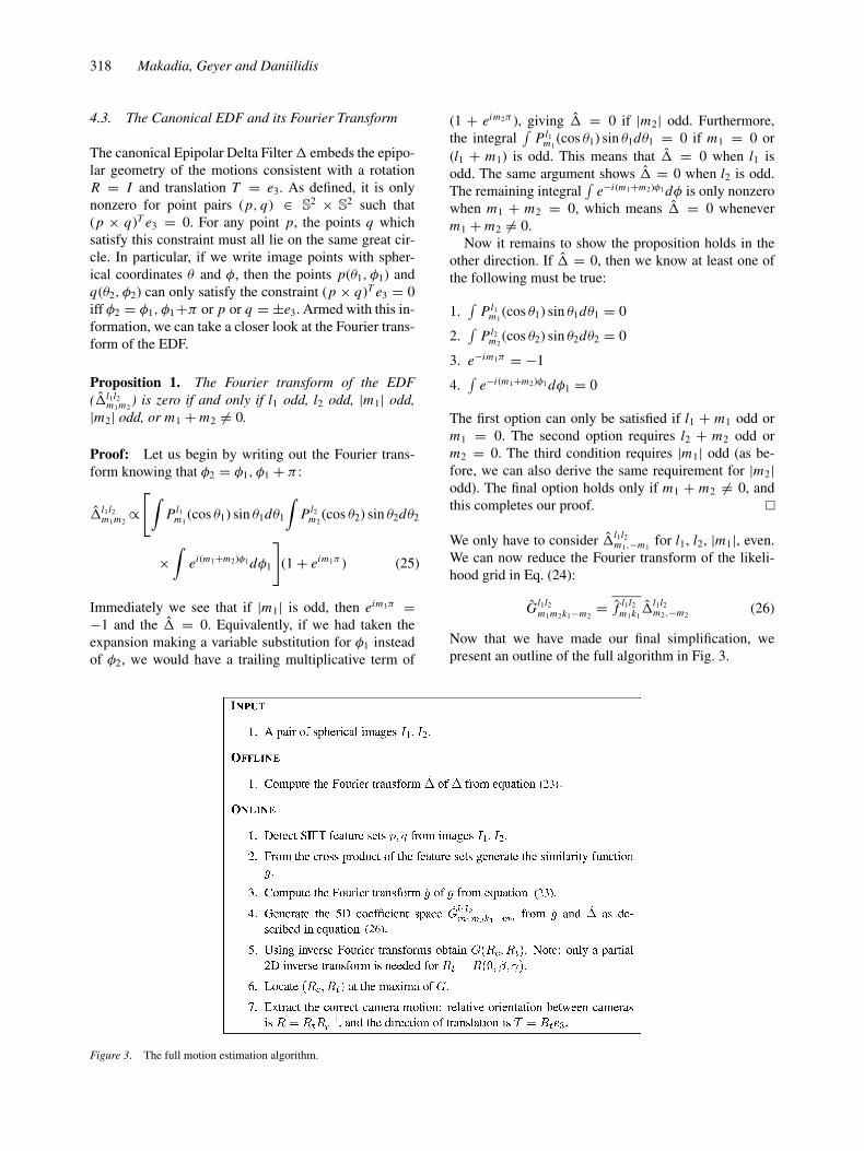
Figure 3. The full motion estimation algorithm.

(1 + eim2π ), giving � = 0 if |m2| odd. Furthermore,the integral

∫Pl1

m1(cos θ1) sin θ1dθ1 = 0 if m1 = 0 or

(l1 + m1) is odd. This means that � = 0 when l1 isodd. The same argument shows � = 0 when l2 is odd.The remaining integral

∫e−i(m1+m2)φ1 dφ is only nonzero

when m1 + m2 = 0, which means � = 0 wheneverm1 + m2 �= 0.

Now it remains to show the proposition holds in theother direction. If � = 0, then we know at least one ofthe following must be true:

1.∫

Pl1m1

(cos θ1) sin θ1dθ1 = 0

2.∫

Pl2m2

(cos θ2) sin θ2dθ2 = 0

3. e−im1π = −1

4.∫

e−i(m1+m2)φ1 dφ1 = 0

The first option can only be satisfied if l1 + m1 odd orm1 = 0. The second option requires l2 + m2 odd orm2 = 0. The third condition requires |m1| odd (as be-fore, we can also derive the same requirement for |m2|odd). The final option holds only if m1 + m2 �= 0, andthis completes our proof.

We only have to consider �l1l2m1,−m1

for l1, l2, |m1|, even.We can now reduce the Fourier transform of the likeli-hood grid in Eq. (24):

Gl1l2

m1m2k1−m2= f l1l2

m1k1�

l1l2m2,−m2

(26)

Now that we have made our final simplification, wepresent an outline of the full algorithm in Fig. 3.


Figure 4. On the left is an spherical image of a great circle. Ideally,

the function values are unity for any point on the circle, and zero oth-

erwise. On the right is a segment of the great circle that intersects

the north and south poles. The segment (which is highlighted on the

left image), This shows the reconstructed function values of the delta

function at the equator (±20◦). The four values of the bandwidth Ltested were 32, 64, 128, and 256. As L increases, the closer the ap-

proximation to an impulse, but because of the discontinuity there is

also a greater overshoot (Gibbs phenomenon).

Figure 5. On the left is a grid depicting the sampling of a spheri-

cal function with bandwidth L = 8. Each white square is one spheri-

cal sample, and the exact location of the sample would be the middle

of the square. The sampling theorem requires 2L uniformly spaced

samples in both coordinates θ ∈ [0, π ] and φ ∈ [0, 2π ), hence there

are 16 rows and 16 columns. The image on the right depicts the po-

sitions on the sphere of all 162 samples. The highlighted samples on

this sphere correspond to the highlighted row of samples in the left im-

age. One visible effect of this sampling theorem is that the sampling is

dense at the north and south poles but sparse at the equator.

5. Discretization and Sampling

There are some issues we must address before we canfinalize the transition from the continuous environment(integration of functions f ∈ L2(S2)) to the discrete

Figure 6. On the left is an image from an omnidirectional sensor, with a field of view of 212◦. In the middle is a spherical image with bandwidth

L = 32 mapped onto the omnidirectional image plane. Each segment in this image corresponds to one pixel in the spherical image. This shows

the quantization or binning effect seen when mapping points from a high-res image to a low-bandwidth spherical function. On the right is the same

effect for a bandwidth L = 40.

setting (images and features). The most obvious concernrelates to the Spherical Fourier Transform of a discretespherical image. In addition to the existence of a sam-pling theorem, we need to be assured that the cost orcomplexity of the transform does not outweigh the ben-efits of replacing the correlation with a multiplication inthe spectral domain. In other words, we require an algo-rithm for a discrete and fast SFT.

The bandwidth L of a spherical function f is thesmallest degree such that f l

m = 0, ∀l ≥ L . Unfor-tunately, the signals we are dealing with (impulseresponses for the similarity function g, and great circlesfor the EDF), do not have a frequency limit. The band-width must be manually selected, and in practical termsdetermines how accurately we wish to approximate ourfunction. Figure 4 shows the approximation of the EDFfor different bandwidth selections. From the figure wesee that even though our similarity function is repre-sented as a sum of spherical impulses, the spectral rep-resentation is smoothed, especially for smaller values ofL .

Given a function with bandwidth L , Driscoll andHealy (1994) (and later refined in Rockmore et al.(2003)), have presented a fast, discrete SFT with asampling theorem that requires 2L uniformly spacedsamples in each spherical coordinate (see Fig. 5). Re-calling Eq. (11), a spherical harmonic is a product of aLegendre polynomial (in the longitudinal parameter θ )with a complex exponential (in the azimuthal parame-ter φ). The SFT amounts to performing many Legen-dre transforms in θ followed by many traditional Fouriertransforms in φ. The more complex of the two is theLegendre transform, which can be performed fast inO(L log2 L) (Driscoll and Healy, 1994). On the orderof L Legendre transforms must be computed, whichgives the total complexity of the SFT as O(L2 log2 L).A similar separation-of-variables approach can be ap-plied to derive a fast and discrete SO(3) Fourier trans-form in O(L3log2L) (Kostelec and Rockmore, 2003),with a similar sampling theorem.


0 1 2 3 4 5 60

20

40

60

80

100

120

140

Estimation errors in rotation

Err

or

(in

deg

rees

)

Standard deviation (in bins)

L = 24L = 32

0 1 2 3 4 5 60

10

20

30

40

50

60

70

80

90Estimation errors in translation

Err

or

(in

deg

rees

)

Standard deviation (in bins)

L = 24L = 32

Figure 7. Results of a simulation testing the robust accumulation in the presence of Gaussian noise. The locations of spherical point correspon-

dences are perturbed with Gaussian noise in each spherical coordinate. The standard deviation of the noise distribution is given here in pixels, and

the error is computed by measuring the distance of the estimated solution from the correct solution in the 5D motion space. On the left is the error

in the estimated rotation (the angular distance between two rotation matrices is computed as arccos((trace(R−11 R2) − 1)/2)), and on the right is the

error in baseline direction. The dashed plots (in red) represent the simulation performed with bandwidth L = 24. In this case, a standard deviation

of one unit corresponds to 7.5◦ and 3.8◦ in the spherical coordinates φ and θ . The solid plots (in blue) are for L = 32, where a standard deviation of

one pixel corresponds to 5.6◦ and 2.8◦ in the spherical coordinates. For this higher bandwidth, the results are still accurate in presence of significant

noise.

Recall from Eq. (9) that we are parameterizing ourmotion space with rotations, which in turn are param-eterized with ZYZ Euler angles. Let us use the anglesα, β, γ , θ , and φ to denote each of the five dimen-sions of our motion space, so that Rc = R(α, β, γ ),Rt = R(0, θ, φ), and α, γ, φ ∈ [0, 2π ), β, θ ∈ [0, π ].If we fix L as the bandwidth of our similarity function gand EDF �, and we follow the algorithm in Fig. 3 usingthe SFT and SOFT routines detailed in Rockmore et al.

Figure 8. Top Left: a parabolic catadioptric image. Bottom: the cor-

responding image on a uniformly sampled spherical grid. As the

parabolic mirror images only a little more than half the sphere, you

can see the lower portion of the spherical image contains no informa-

tion. Top Right: the spherical image as it would appear on the surface

of the sphere.

(2003) and Kostelec and Rockmore (2003), the angles α,γ , and φ will be sampled at

α j , γ j , φ j = π j

L, j = 0, 1, . . . , 2L − 1 (27)

The angles β, and θ will be sampled at

βk, θk = π (2k + 1)

4L, k = 0, 1, . . . , 2L − 1 (28)

The total number of samples in G is thus 32L5. In prac-tice, this forces us to select lower values for L , such as32. Although we are capturing high resolution imagesand locating image features with sub-pixel accuracy, theeffective resolution of one spherical image is just 2L ×2L . The experiment detailed in Fig. 7 shows just how ouralgorithm reacts when the feature locations are affectedby Gaussian noise when using such “low-resolution”spherical images. Figure 6 shows the relationship be-tween the uniform angular spacing of the spherical sam-ples and the original image domains of different single-viewpoint cameras. It is clear for small L many pix-els from a high-res perspective or omnidirectional im-age will map to the same spherical sample, and since wewill detect features on the original images we must clar-ify how to generate a discrete version of our similarityfunction g.

The sampling theorem requires 2L samples in eachangle, which means every spherical function must have4L2 samples, and g must therefore have 16L4 samples.Let us write (p j , qk), j, k = 1, 2, . . . , 4L2 for the sam-ples of g. Assume we are given two input images I1, I2


8 12 16 20 24 28 320

50

100

150

200

250

Bandwidth (L)

Execu

tio

n t

ime (

seco

nd

s)

Figure 9. Timings of our algorithm for various bandwidth choices.

The execution times are for step 3 through step 7 (see Fig. 3).

on which we detect N1 and N2 features, respectively. Wedenote Q as the set of all possible feature pairs (note thatQ has N1 N2 elements), and each element of Q has an as-sociated weight given by Eq. (2) (or Eq. (3)). The valueof the discrete similarity function at a sample (p j , qk)

00.5

11.5

22.5

33.5

44.5

00.5

0

YX

Translation along X axis

Z

RADON

RANSAC

0 0.05 0.1 0.15 0.2 0.25

0

0.05

Y

Z

RADON

RANSAC

φ

θ

Radon space (translational slice)

10 20 30 40 50 60

10

20

30

40

50

60

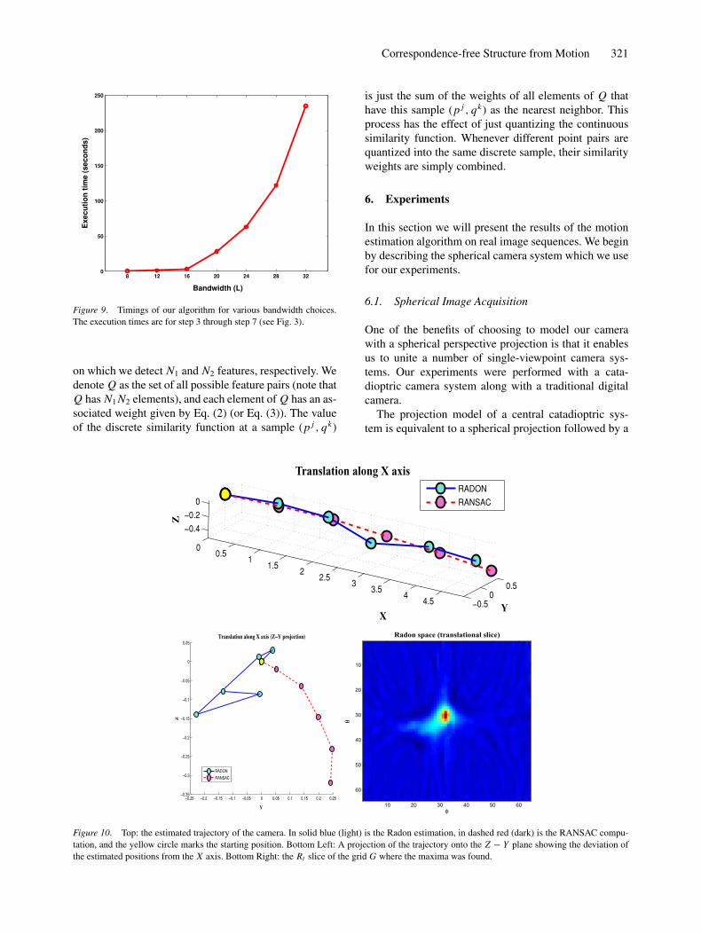
Figure 10. Top: the estimated trajectory of the camera. In solid blue (light) is the Radon estimation, in dashed red (dark) is the RANSAC compu-

tation, and the yellow circle marks the starting position. Bottom Left: A projection of the trajectory onto the Z − Y plane showing the deviation of

the estimated positions from the X axis. Bottom Right: the Rt slice of the grid G where the maxima was found.

is just the sum of the weights of all elements of Q thathave this sample (p j , qk) as the nearest neighbor. Thisprocess has the effect of just quantizing the continuoussimilarity function. Whenever different point pairs arequantized into the same discrete sample, their similarityweights are simply combined.

6. Experiments

In this section we will present the results of the motionestimation algorithm on real image sequences. We beginby describing the spherical camera system which we usefor our experiments.

6.1. Spherical Image Acquisition

One of the benefits of choosing to model our camerawith a spherical perspective projection is that it enablesus to unite a number of single-viewpoint camera sys-tems. Our experiments were performed with a cata-dioptric camera system along with a traditional digitalcamera.

The projection model of a central catadioptric sys-tem is equivalent to a spherical projection followed by a


00.5

100.5

0

0.5

1

1.5

2

2.5

3

3.5

4

4.5

X

Translation along Z axis

Y

Z

RADON

RANSAC

0 0.05 0.1 0.15 0.2 0.25 0.3

0

0.05

0.1

X

Y

RADON

RANSAC

φ

θ

Radon space (translational slice)

10 20 30 40 50 60

10

20

30

40

50

60

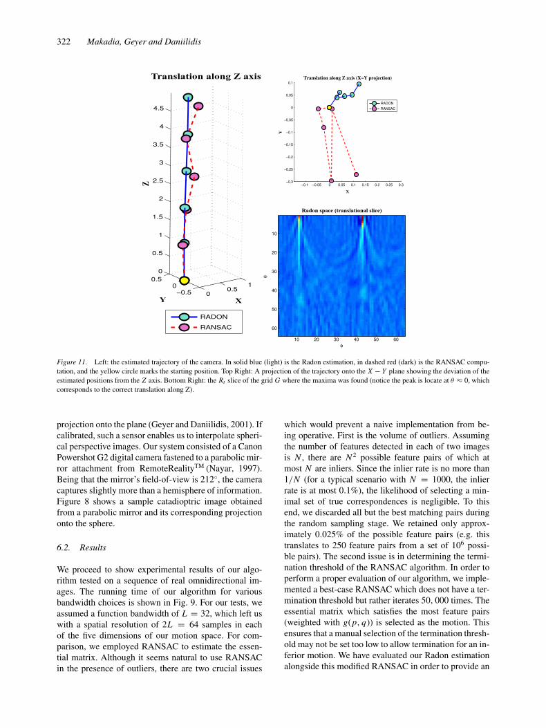
Figure 11. Left: the estimated trajectory of the camera. In solid blue (light) is the Radon estimation, in dashed red (dark) is the RANSAC compu-

tation, and the yellow circle marks the starting position. Top Right: A projection of the trajectory onto the X − Y plane showing the deviation of the

estimated positions from the Z axis. Bottom Right: the Rt slice of the grid G where the maxima was found (notice the peak is locate at θ ≈ 0, which

corresponds to the correct translation along Z).

projection onto the plane (Geyer and Daniilidis, 2001). Ifcalibrated, such a sensor enables us to interpolate spheri-cal perspective images. Our system consisted of a CanonPowershot G2 digital camera fastened to a parabolic mir-ror attachment from RemoteRealityTM (Nayar, 1997).Being that the mirror’s field-of-view is 212◦, the cameracaptures slightly more than a hemisphere of information.Figure 8 shows a sample catadioptric image obtainedfrom a parabolic mirror and its corresponding projectiononto the sphere.

6.2. Results

We proceed to show experimental results of our algo-rithm tested on a sequence of real omnidirectional im-ages. The running time of our algorithm for variousbandwidth choices is shown in Fig. 9. For our tests, weassumed a function bandwidth of L = 32, which left uswith a spatial resolution of 2L = 64 samples in eachof the five dimensions of our motion space. For com-parison, we employed RANSAC to estimate the essen-tial matrix. Although it seems natural to use RANSACin the presence of outliers, there are two crucial issues

which would prevent a naive implementation from be-ing operative. First is the volume of outliers. Assumingthe number of features detected in each of two imagesis N , there are N 2 possible feature pairs of which atmost N are inliers. Since the inlier rate is no more than1/N (for a typical scenario with N = 1000, the inlierrate is at most 0.1%), the likelihood of selecting a min-imal set of true correspondences is negligible. To thisend, we discarded all but the best matching pairs duringthe random sampling stage. We retained only approx-imately 0.025% of the possible feature pairs (e.g. thistranslates to 250 feature pairs from a set of 106 possi-ble pairs). The second issue is in determining the termi-nation threshold of the RANSAC algorithm. In order toperform a proper evaluation of our algorithm, we imple-mented a best-case RANSAC which does not have a ter-mination threshold but rather iterates 50, 000 times. Theessential matrix which satisfies the most feature pairs(weighted with g(p, q)) is selected as the motion. Thisensures that a manual selection of the termination thresh-old may not be set too low to allow termination for an in-ferior motion. We have evaluated our Radon estimationalongside this modified RANSAC in order to provide an


00.5

1

0

0.5

1

1.5

2

2.5

0

Circular motion

X

Y

Z

RADON

RANSAC

0 0.5 10

0.5

1

1.5

2

2.5

X

Y

RADON

RANSAC

0 0.5 10

0.5

1

1.5

2

2.5

X

Y

RADON

RANSAC

GROUND TRUTH

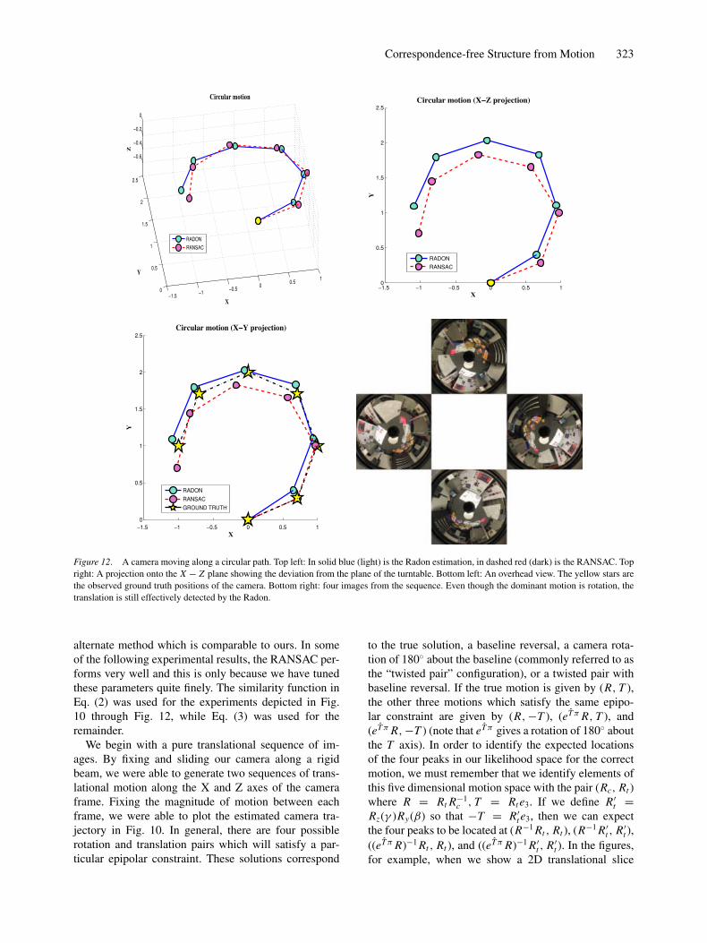
Figure 12. A camera moving along a circular path. Top left: In solid blue (light) is the Radon estimation, in dashed red (dark) is the RANSAC. Top

right: A projection onto the X − Z plane showing the deviation from the plane of the turntable. Bottom left: An overhead view. The yellow stars are

the observed ground truth positions of the camera. Bottom right: four images from the sequence. Even though the dominant motion is rotation, the

translation is still effectively detected by the Radon.

alternate method which is comparable to ours. In someof the following experimental results, the RANSAC per-forms very well and this is only because we have tunedthese parameters quite finely. The similarity function inEq. (2) was used for the experiments depicted in Fig.10 through Fig. 12, while Eq. (3) was used for theremainder.

We begin with a pure translational sequence of im-ages. By fixing and sliding our camera along a rigidbeam, we were able to generate two sequences of trans-lational motion along the X and Z axes of the cameraframe. Fixing the magnitude of motion between eachframe, we were able to plot the estimated camera tra-jectory in Fig. 10. In general, there are four possiblerotation and translation pairs which will satisfy a par-ticular epipolar constraint. These solutions correspond

to the true solution, a baseline reversal, a camera rota-tion of 180◦ about the baseline (commonly referred to asthe “twisted pair” configuration), or a twisted pair withbaseline reversal. If the true motion is given by (R, T ),the other three motions which satisfy the same epipo-

lar constraint are given by (R, −T ), (eT π R, T ), and

(eT π R, −T ) (note that eT π gives a rotation of 180◦ aboutthe T axis). In order to identify the expected locationsof the four peaks in our likelihood space for the correctmotion, we must remember that we identify elements ofthis five dimensional motion space with the pair (Rc, Rt )where R = Rt R−1

c , T = Rt e3. If we define R′t =

Rz(γ )Ry(β) so that −T = R′t e3, then we can expect

the four peaks to be located at (R−1 Rt , Rt ), (R−1 R′t , R′

t ),

((eT π R)−1 Rt , Rt ), and ((eT π R)−1 R′t , R′

t ). In the figures,for example, when we show a 2D translational slice


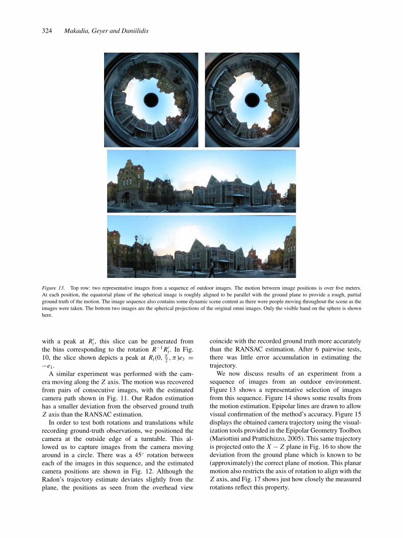
Figure 13. Top row: two representative images from a sequence of outdoor images. The motion between image positions is over five meters.

At each position, the equatorial plane of the spherical image is roughly aligned to be parallel with the ground plane to provide a rough, partial

ground truth of the motion. The image sequence also contains some dynamic scene content as there were people moving throughout the scene as the

images were taken. The bottom two images are the spherical projections of the original omni images. Only the visible band on the sphere is shown

here.

with a peak at R′t , this slice can be generated from

the bins corresponding to the rotation R−1 R′t . In Fig.

10, the slice shown depicts a peak at Rt (0, π2, π )e3 =

−e1.A similar experiment was performed with the cam-

era moving along the Z axis. The motion was recoveredfrom pairs of consecutive images, with the estimatedcamera path shown in Fig. 11. Our Radon estimationhas a smaller deviation from the observed ground truthZ axis than the RANSAC estimation.

In order to test both rotations and translations whilerecording ground-truth observations, we positioned thecamera at the outside edge of a turntable. This al-lowed us to capture images from the camera movingaround in a circle. There was a 45◦ rotation betweeneach of the images in this sequence, and the estimatedcamera positions are shown in Fig. 12. Although theRadon’s trajectory estimate deviates slightly from theplane, the positions as seen from the overhead view

coincide with the recorded ground truth more accuratelythan the RANSAC estimation. After 6 pairwise tests,there was little error accumulation in estimating thetrajectory.

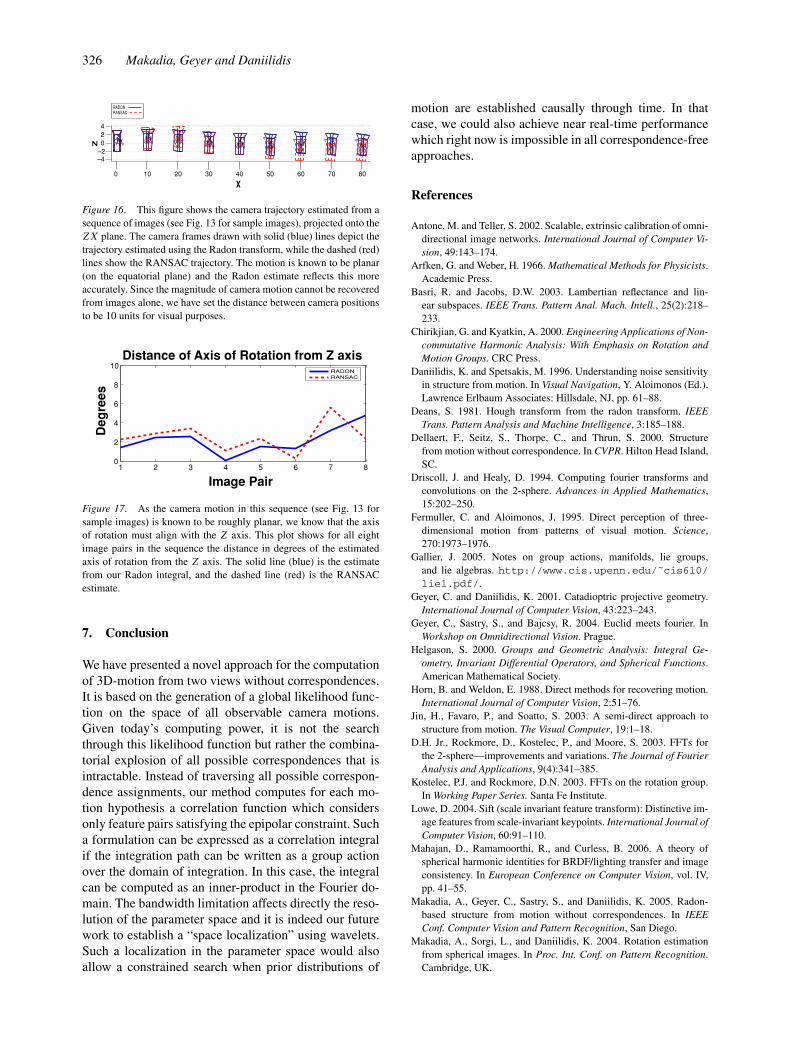
We now discuss results of an experiment from asequence of images from an outdoor environment.Figure 13 shows a representative selection of imagesfrom this sequence. Figure 14 shows some results fromthe motion estimation. Epipolar lines are drawn to allowvisual confirmation of the method’s accuracy. Figure 15displays the obtained camera trajectory using the visual-ization tools provided in the Epipolar Geometry Toolbox(Mariottini and Prattichizzo, 2005). This same trajectoryis projected onto the X − Z plane in Fig. 16 to show thedeviation from the ground plane which is known to be(approximately) the correct plane of motion. This planarmotion also restricts the axis of rotation to align with theZ axis, and Fig. 17 shows just how closely the measuredrotations reflect this property.


Figure 14. On the top row are a pair of images from a sequence for which the motion was estimated. The bottom two rows show the images after

they have been rotationally aligned. Epipolar circles have been overlaid onto the images. Since the images have been rotationally aligned, points

which lie along these circles in one image will lie along the same circle in the second image. The intersection of these circles mark the focus of

expansion and contraction, which define the direction of translation between this image pair. The rotation between image pairs was estimated at

approximately 45◦, and as the focus of expansion shows the translation was roughly in the equatorial plane.

0

10

20

30

40

50

60

70

80

0–2

–2–4

2

024

Xc

ZcXc

Zc

YcY

cXc

ZcXc

Zc

YcY

cXc

ZcXc

Zc

YcY

cX

cXc

ZcZc

YcY

cXcXcZ

c

ZcY

c

Yc

XcXc

ZcZcY

cYc

X

XcXc

Zc

ZcY

cY

c

Xc

XcZ

cZ

cYc

Yc

Xc

Xc

Zc

Zc

Yc

Yc

Z

Y

RADONRANSAC

Figure 15. This figure shows the camera trajectory estimated from a sequence of images (see Fig. 13 for sample images). The camera frames drawn

with solid (blue) lines depict the trajectory estimated using the Radon transform, while the dashed (red) lines show the RANSAC trajectory. In this

sequence the motion is known to be approximately planar in the equatorial plane. Since the magnitude of camera motion cannot be recovered from

pairs of images alone, we have fixed the distance between camera positions to be 10 units for visual purposes.


0 10 20 30 40 50 60 70 80

0–2–4

24

Xc

Xc

Zc

Zc

Yc

Yc

Xc

Xc

Zc

Zc

Yc

Yc

Xc

Xc

Zc

Zc

Yc

Yc

XcX

c

ZcZ

cYcY

c

Xc

Xc

Zc

Zc

X

Yc

Yc

Xc

Xc

Zc

ZcY

cY

cX

c

Xc

Zc

Zc

Yc

YcX

cX

c

ZcZcY

cY

cXc

Xc

Zc

ZcYc

YcZ

RADONRANSAC

Figure 16. This figure shows the camera trajectory estimated from a

sequence of images (see Fig. 13 for sample images), projected onto the

Z X plane. The camera frames drawn with solid (blue) lines depict the

trajectory estimated using the Radon transform, while the dashed (red)

lines show the RANSAC trajectory. The motion is known to be planar

(on the equatorial plane) and the Radon estimate reflects this more

accurately. Since the magnitude of camera motion cannot be recovered

from images alone, we have set the distance between camera positions

to be 10 units for visual purposes.

1 2 3 4 5 6 7 80

2

4

6

8

10Distance of Axis of Rotation from Z axis

Deg

rees

Image Pair

RADONRANSAC

Figure 17. As the camera motion in this sequence (see Fig. 13 for

sample images) is known to be roughly planar, we know that the axis

of rotation must align with the Z axis. This plot shows for all eight

image pairs in the sequence the distance in degrees of the estimated

axis of rotation from the Z axis. The solid line (blue) is the estimate

from our Radon integral, and the dashed line (red) is the RANSAC

estimate.

7. Conclusion

We have presented a novel approach for the computationof 3D-motion from two views without correspondences.It is based on the generation of a global likelihood func-tion on the space of all observable camera motions.Given today’s computing power, it is not the searchthrough this likelihood function but rather the combina-torial explosion of all possible correspondences that isintractable. Instead of traversing all possible correspon-dence assignments, our method computes for each mo-tion hypothesis a correlation function which considersonly feature pairs satisfying the epipolar constraint. Sucha formulation can be expressed as a correlation integralif the integration path can be written as a group actionover the domain of integration. In this case, the integralcan be computed as an inner-product in the Fourier do-main. The bandwidth limitation affects directly the reso-lution of the parameter space and it is indeed our futurework to establish a “space localization” using wavelets.Such a localization in the parameter space would alsoallow a constrained search when prior distributions of

motion are established causally through time. In thatcase, we could also achieve near real-time performancewhich right now is impossible in all correspondence-freeapproaches.

References

Antone, M. and Teller, S. 2002. Scalable, extrinsic calibration of omni-

directional image networks. International Journal of Computer Vi-sion, 49:143–174.

Arfken, G. and Weber, H. 1966. Mathematical Methods for Physicists.

Academic Press.

Basri, R. and Jacobs, D.W. 2003. Lambertian reflectance and lin-

ear subspaces. IEEE Trans. Pattern Anal. Mach. Intell., 25(2):218–

233.

Chirikjian, G. and Kyatkin, A. 2000. Engineering Applications of Non-commutative Harmonic Analysis: With Emphasis on Rotation andMotion Groups. CRC Press.

Daniilidis, K. and Spetsakis, M. 1996. Understanding noise sensitivity

in structure from motion. In Visual Navigation, Y. Aloimonos (Ed.).

Lawrence Erlbaum Associates: Hillsdale, NJ, pp. 61–88.

Deans, S. 1981. Hough transform from the radon transform. IEEETrans. Pattern Analysis and Machine Intelligence, 3:185–188.

Dellaert, F., Seitz, S., Thorpe, C., and Thrun, S. 2000. Structure

from motion without correspondence. In CVPR. Hilton Head Island,

SC.

Driscoll, J. and Healy, D. 1994. Computing fourier transforms and

convolutions on the 2-sphere. Advances in Applied Mathematics,

15:202–250.

Fermuller, C. and Aloimonos, J. 1995. Direct perception of three-

dimensional motion from patterns of visual motion. Science,

270:1973–1976.

Gallier, J. 2005. Notes on group actions, manifolds, lie groups,

and lie algebras. http://www.cis.upenn.edu/˜cis610/lie1.pdf/.

Geyer, C. and Daniilidis, K. 2001. Catadioptric projective geometry.

International Journal of Computer Vision, 43:223–243.

Geyer, C., Sastry, S., and Bajcsy, R. 2004. Euclid meets fourier. In

Workshop on Omnidirectional Vision. Prague.

Helgason, S. 2000. Groups and Geometric Analysis: Integral Ge-ometry, Invariant Differential Operators, and Spherical Functions.

American Mathematical Society.

Horn, B. and Weldon, E. 1988. Direct methods for recovering motion.

International Journal of Computer Vision, 2:51–76.

Jin, H., Favaro, P., and Soatto, S. 2003. A semi-direct approach to

structure from motion. The Visual Computer, 19:1–18.

D.H. Jr., Rockmore, D., Kostelec, P., and Moore, S. 2003. FFTs for

the 2-sphere—improvements and variations. The Journal of FourierAnalysis and Applications, 9(4):341–385.

Kostelec, P.J. and Rockmore, D.N. 2003. FFTs on the rotation group.

In Working Paper Series. Santa Fe Institute.

Lowe, D. 2004. Sift (scale invariant feature transform): Distinctive im-

age features from scale-invariant keypoints. International Journal ofComputer Vision, 60:91–110.

Mahajan, D., Ramamoorthi, R., and Curless, B. 2006. A theory of

spherical harmonic identities for BRDF/lighting transfer and image

consistency. In European Conference on Computer Vision, vol. IV,

pp. 41–55.

Makadia, A., Geyer, C., Sastry, S., and Daniilidis, K. 2005. Radon-

based structure from motion without correspondences. In IEEEConf. Computer Vision and Pattern Recognition, San Diego.

Makadia, A., Sorgi, L., and Daniilidis, K. 2004. Rotation estimation

from spherical images. In Proc. Int. Conf. on Pattern Recognition.

Cambridge, UK.


Mariottini, G. and Prattichizzo, D. 2005. EGT: A toolbox for multiple

view geometry and visual servoing. IEEE Robotics and AutomationMagazine, 3(12).

Maslen, D. and Rockmore, D. 1995. Generalized FFTs—a survey of

some recent results. In Proceedings of the DIMACS Workshop onGroups and Computation.

Nayar, S. 1997. Catadioptric omnidirectional camera. In IEEE Conf.Computer Vision and Pattern Recognition. Puerto Rico, pp. 482–

488.

Negahdaripour, S. and Horn, B. 1987. Direct passive navigation.

IEEE Trans. Pattern Analysis and Machine Intelligence, 9:168–

176.

Oliensis, J. 2000. A critique of structure from motion algo-

rithms. Computer Vision and Image Understanding, 80:172–

214.

Roy, S. and Cox, I. 1996. Motion without structure. In Proc. Int. Conf.on Pattern Recognition. Vienna, Austria.

Schroder, P. and Sweldens, W. 1995. Spherical wavelets: Efficiently

representing functions on the sphere. In SIGGRAPH ’95: Proceed-ings of the 22nd annual conference on Computer graphics and in-teractive techniques. ACM Press: New York. pp. 161–172.

Shi, J. and Malik, J. 1998. Motion segmentation and tracking using

normalized cuts. In Proc. Int. Conf. on Computer Vision.

Sugiura, M. 1990. Unitary Representations and Harmonic Analysis:An Introduction. second edition. North Holland, Amsterdam.

Szeliski, R. and Kang, S.B. 1995. Direct methods for visual scene

reconstruction. In IEEE Workshop on Representations of VisualScenes, pp. 26–33.

Vidal, R. and Ma, Y. 2004. A unified algebraic approach to 2-D and

3-D motion segmentation. In European Conference on ComputerVision, pp. 1–15.

Wexler, Y., Fitzgibbon, A., and Zisserman, A. 2003. Learning epipolar

geometry from image sequences. In IEEE Conf. Computer Visionand Pattern Recognition. Wisconsin.

correspondence-free structure from motionkostas/mypub.dir/makadia07ijcv.pdfcorrespondence-free...

Documents